The PDF4LHC Working Group Interim Report

Sergey Alekhin1,2, Simone Alioli1, Richard D. Ball3, Valerio Bertone4, Johannes Blumlein1, MichielBotje5, Jon Butterworth6, Francesco Cerutti7, Amanda Cooper-Sarkar8 , Albert de Roeck9,Luigi Del Debbio3, Joel Feltesse10, Stefano Forte11, Alexander Glazov12, Alberto Guffanti4, ClaireGwenlan8, Joey Huston13, Pedro Jimenez-Delgado14 , Hung-Liang Lai15, Jose I. Latorre7, RonanMcNulty16, Pavel Nadolsky17, Sven Olaf Moch1, Jon Pumplin13, Voica Radescu18, Juan Rojo11,Torbjorn Sjostrand19 , W.J. Stirling20, Daniel Stump13, Robert S. Thorne6, Maria Ubiali21, AlessandroVicini11, Graeme Watt22, C.-P. Yuan131 Deutsches Elektronen-Synchrotron, DESY, Platanenallee 6, D-15738 Zeuthen, Germany2 Institute for High Energy Physics, IHEP, Pobeda 1, 142281 Protvino, Russia3 School of Physics and Astronomy, University of Edinburgh, JCMB, KB, Mayfield Rd, EdinburghEH9 3JZ, Scotland4 Physikalisches Institut, Albert-Ludwigs-Universitat Freiburg, Hermann-Herder-Straße 3, D-79104Freiburg i. B., Germany5 NIKHEF, Science Park, Amsterdam, The Netherlands6 Department of Physics and Astronomy, University College, London, WC1E 6BT, UK7 Departament d’Estructura i Constituents de la Materia, Universitat de Barcelona, Diagonal 647,E-08028 Barcelona, Spain8 Department of Physics, Oxford University, Denys WilkinsonBldg, Keble Rd, Oxford, OX1 3RH, UK9 CERN, CH–1211 Geneve 23, Switzerland; Antwerp University, B–2610 Wilrijk, Belgium; Universityof California Davis, CA, USA10 CEA, DSM/IRFU, CE-Saclay, Gif-sur-Yvetee, France11 Dipartimento di Fisica, Universita di Milano and INFN, Sezione di Milano, Via Celoria 16, I-20133Milano, Italy12 Deutsches Elektronensynchrotron DESY Notkestraße 85 D–22607 Hamburg, Germany13 Physics and Astronomy Department, Michigan State University, East Lansing, MI 48824, USA14 Institut fur Theoretische Physik, Universitat Zurich,CH-8057 Zurich, Switzerland15 Taipei Municipal University of Education, Taipei, Taiwan16 School of Physics, University College Dublin Science Centre North, UCD Belfeld, Dublin 4, Ireland17 Department of Physics, Southern Methodist University, Dallas, TX 75275-0175, USA18 Physikalisches Institut, Universitat Heidelberg Philosophenweg 12, D–69120 Heidelberg, Germany19 Department of Astronomy and Theoretical Physics, Lund University, Solvegatan 14A, S-223 62Lund, Sweden20 Cavendish Laboratory, University of Cambridge, CB3 OHE, UK21 Institut fur Theoretische Teilchenhysik und Kosmologie,RWTH Aachen University, D-52056Aachen, Germany22 Theory Group, Physics Department, CERN, CH-1211 Geneva 23,Switzerland

Abstract

This document is intended as a study of benchmark cross sections at the LHC(at 7 TeV) at NLO using modern PDFs currently available from the 6 PDFfitting groups that have participated in this exercise. It also contains a succinctuser guide to the computation of PDFs, uncertainties and correlations usingavailable PDF sets.

A companion note provides an interim summary of the current recommenda-tions of the PDF4LHC working group for the use of parton distribution func-tions (PDFs) and of PDF uncertainties at the LHC, for cross section and crosssection uncertainty calculations.

2

Contents

1. Introduction 4

2. PDF determinations - experimental uncertainties 5

2.1 Features, tradeoffs and choices . . . . . . . . . . . . . . . . . . . .. . . . . . . . . . . 5

2.11 Data Set . . . . . . . . . . . . . . . . . . . . . . . . . . . . . . . . . . . . . . . 5

2.12 Statistical treatment . . . . . . . . . . . . . . . . . . . . . . . . . . .. . . . . . 5

2.13 Parton parametrization . . . . . . . . . . . . . . . . . . . . . . . . . .. . . . . 6

2.2 PDF delivery and usage . . . . . . . . . . . . . . . . . . . . . . . . . . . . .. . . . . . 7

2.21 Computation of Hessian PDF uncertainties . . . . . . . . . . .. . . . . . . . . 7

2.22 Computation of Monte Carlo PDF uncertainties . . . . . . . .. . . . . . . . . . 8

3. PDF determinations - Theoretical uncertainties 10

3.1 The value ofαs and its uncertainty . . . . . . . . . . . . . . . . . . . . . . . . . . . . . 10

3.2 Computation of PDF+αs uncertainties . . . . . . . . . . . . . . . . . . . . . . . . . . . 11

3.21 CTEQ - Combined PDF andαs uncertainties . . . . . . . . . . . . . . . . . . . 12

3.22 MSTW - Combined PDF andαs uncertainties . . . . . . . . . . . . . . . . . . . 12

3.23 HERAPDF -αs, model and parametrization uncertainties . . . . . . . . . . . . 13

3.24 NNPDF - Combined PDF andαs uncertainties . . . . . . . . . . . . . . . . . . 13

4. PDF correlations 15

4.1 PDF correlations in the Hessian approach . . . . . . . . . . . . .. . . . . . . . . . . . 15

4.2 PDF correlations in the Monte Carlo approach . . . . . . . . . .. . . . . . . . . . . . . 17

5. The PDF4LHC benchmarks 18

5.1 Comparison between benchmark predictions . . . . . . . . . . .. . . . . . . . . . . . . 19

5.2 Tables of results from each PDF set . . . . . . . . . . . . . . . . . . .. . . . . . . . . 22

5.21 ABMK09 NLO 5 Flavours . . . . . . . . . . . . . . . . . . . . . . . . . . . . .22

5.22 CTEQ6.6 . . . . . . . . . . . . . . . . . . . . . . . . . . . . . . . . . . . . . . 24

5.23 GJR . . . . . . . . . . . . . . . . . . . . . . . . . . . . . . . . . . . . . . . . . 26

5.24 HERAPDF1.0 . . . . . . . . . . . . . . . . . . . . . . . . . . . . . . . . . . . 27

5.25 MSTW2008 . . . . . . . . . . . . . . . . . . . . . . . . . . . . . . . . . . . . 28

5.26 NNPDF2.0 . . . . . . . . . . . . . . . . . . . . . . . . . . . . . . . . . . . . . 29

5.3 Comparison ofW+,W−, Zo rapidity distributions . . . . . . . . . . . . . . . . . . . . 31

6. Summary 31

3

1. Introduction

The LHC experiments are currently producing cross sectionsfrom the 7 TeV data, and thus need accuratepredictions for these cross sections and their uncertainties at NLO and NNLO. Crucial to the predictionsand their uncertainties are the parton distribution functions (PDFs) obtained from global fits to data fromdeep-inelastic scattering, Drell-Yan and jet data. A number of groups have produced publicly availablePDFs using different data sets and analysis frameworks. It is one of the charges of the PDF4LHC workinggroup to evaluate and understand differences among the PDF sets to be used at the LHC, and to providea protocol for both experimentalists and theorists to use the PDF sets to calculate central cross sectionsat the LHC, as well as to estimate their PDF uncertainty. Thiscurrent note is intended to be an interimsummary of our level of understanding of NLO predictions as the first LHC cross sections at 7 TeV arebeing produced1. The intention is to modify this note as improvements in data/understanding warrant.

For the purpose of increasing our quantitative understanding of the similarities and differencesbetween available PDF determinations, a benchmarking exercise between the different groups was per-formed. This exercise was very instructive in understanding many differences in the PDF analyses:different input data, different methodologies and criteria for determining uncertainties, different waysof parametrizing PDFs, different number of parametrized PDFs, different treatments of heavy quarks,different perturbative orders, different ways of treatingαs (as an input or as a fit parameter), differentvalues of physical parameters such asαs itself and heavy quark masses, and more. This exercise wasalso very instructive in understanding where the PDFs agreeand where they disagree: it established abroad agreement of PDFs (and uncertainties) obtained from data sets of comparable size and it singledout relevant instances of disagreement and of dependence ofthe results on assumptions or methodology.

The outline of this interim report is as follows. The first three sections are devoted to a descriptionof current PDF sets and their usage. In Sect. 2. we present several modern PDF determinations, withspecial regard to the way PDF uncertainties are determined.First we summarize the main featuresof various sets, then we provide an explicit users’ guide forthe computation of PDF uncertainties. InSect. 3. we discuss theoretical uncertainties on PDFs. We first introduce various theoretical uncertainties,then we focus on the uncertainty related to the strong coupling and also in this case we give both apresentation of choices made by different groups and a users’ guide for the computation of combinedPDF+αs uncertainties. Finally in Sect. 4. we discuss PDF correlations and the way they can be computed.

In Sect. 5. we introduce the settings for the PDF4LHC benchmarks on LHC observables, presentthe results from the different groups and compare their predictions for important LHC observables at 7TeV at NLO. In Sect. 6. we conclude and briefly discuss prospects for future developments.

1Comparisons at NNLO forW ,Z and Higgs production can be found in ref. [1]

4

2. PDF determinations - experimental uncertainties

Experimental uncertainties of PDFs determined in global fits (usually called “PDF uncertainties” forshort) reflect three aspects of the analysis, and differ because of different choices made in each of theseaspects: (1) the choice of data set; (2) the type of uncertainty estimator used which is used to deter-mine the uncertainties and which also determines the way in which PDFs are delivered to the user; (3)the form and size of parton parametrization. First, we briefly discuss the available options for eachof these aspects (at least, those which have been explored bythe various groups discussed here) andsummarize the choices made by each group; then, we provide a concise user guide for the determina-tion of PDF uncertainties for available fits. We will in particular discuss the following PDF sets (whenseveral releases are available the most recent published ones are given in parenthesis in each case):ABKM/ABM [2, 3], CTEQ/CT (CTEQ6.6 [4], CT10 [5]), GJR [6, 7],HERAPDF (HERAPDF1.0 [8]),MSTW (MSTW08 [9]), NNPDF (NNPDF2.0 [10]). There is a significant time-lag between the develop-ment of a new PDF and the wide adoption of its use by experimental collaborations, so in some cases,we report not on the most up-to-date PDF from a particular group, but instead on the most widely-used.

2.1 Features, tradeoffs and choices

2.11 Data Set

There is a clear tradeoff between the size and the consistency of a data set: a wider data set containsmore information, but data coming from different experiment may be inconsistent to some extent. Thechoices made by the various groups are the following:

• The CTEQ, MSTW and NNPDF data sets considered here include both electroproduction andhadroproduction data, in each case both from fixed-target and collider experiments. The electro-production data include electron, muon and neutrino deep–inelastic scattering data (both inclusiveand charm production). The hadroproduction data include Drell-Yan (fixed target virtual photonand colliderW andZ production) and jet production2.

• The GJR data set includes electroproduction data from fixed-target and collider experiments, anda smaller set of hadroproduction data. The electroproduction data include electron and muoninclusive deep–inelastic scattering data, and deep-inelastic charm production from charged leptonsand neutrinos. The hadroproduction data includes fixed–target virtual photon Drell-Yan productionand Tevatron jet production.

• The ABKM/ABM data sets include electroproduction from fixed-target and collider experiments,and fixed–target hadroproduction data. The electroproduction data include electron, muon andneutrino deep–inelastic scattering data (both inclusive and charm production). The hadropro-duction data include fixed–target virtual photon Drell-Yanproduction. The most recent version,ABM10 [11], includes Tevatron jet data.

• The HERAPDF data set includes all HERA deep-inelastic inclusive data.

2.12 Statistical treatment

Available PDF determinations fall in two broad categories:those based on a Hessian approach and thosewhich use a Monte Carlo approach. The delivery of PDFs is different in each case and will be discussedin Sect. 2.2.

Within the Hessian method, PDFs are determined by minimizing a suitable log-likelihoodχ2 func-tion. Different groups may use somewhat different definitions ofχ2, for example, by including entirely,

2Although the comparisons included in this note are only at NLO,we note that, to date, the inclusive jet cross section, unlikethe other processes in the list above, has been calculated only to NLO, and not to NNLO. This may have an impact on theprecision of NNLO global PDF fits that include inclusive jet data.

5

or only partially, correlated systematic uncertainties. While some groups account for correlated uncer-tainties by means of a covariance matrix, other groups treatsome correlated systematics (specifically butnot exclusively normalization uncertanties) as a shift of data, with a penalty term proportional to somepower of the shift parameter added to theχ2. The reader is referred to the original papers for the precisedefinition adopted by each group, but it should be born in mindthat because of all these differences,values of theχ2 quoted by different groups are in general only roughly comparable.

With the covariance matrix approach, we can defineχ2 = 1Ndat

∑

i,j(di − di)covij(dj − dj), di

are data,di theoretical predictions,Ndat is the number of data points (note the inclusion of the factor1

Ndatin the definition) andcovij is the covariance matrix. Different groups may use somewhatdifferent

definitions of the covariance matrix, by including entirelyor only partially correlated uncertainties. Thebest fit is the point in parameter space at whichχ2 is minimum, while PDF uncertainties are foundby diagonalizing the (Hessian) matrix of second derivatives of theχ2 at the minimum (see Fig. 1) andthen determining the range of each orthonormal Hessian eigenvector which corresponds to a prescribedincrease of theχ2 function with respect to the minimum.

In principle, the variation of theχ2 which corresponds to a 68% confidence (one sigma) is∆χ2 =1. However, a larger variation∆χ2 = T 2, with T > 1 a suitable “tolerance” parameter [12, 13, 14]may turn out to be necessary for more realistic error estimates for fits containing a wide variety of in-put processes/data, and in particular in order for each individual experiment which enters the global fitto be consistent with the global best fit to one sigma (or some other desired confidence level such as90%). Possible reasons why this is necessary could be related to data inconsistencies or incompatibili-ties, underestimated experimental systematics, insufficiently flexible parton parametrizations, theoreticaluncertainties or approximation in the PDF extraction. At present, HERAPDF and ABKM use∆χ2 = 1,GJR usesT ≈ 4.7 at one sigma (corresponding toT ≈ 7.5 at 90% c.l.), CTEQ6.6 usesT = 10 at90% c.l. (corresponding toT ≈ 6.1 to one sigma) and MSTW08 uses a dynamical tolerance [9], i.e.adifferent value ofT for each eigenvector, with values for one sigma ranging fromT ≈ 1 to T ≈ 6.5 andmost values being2 < T < 5.

Within the NNPDF method, PDFs are determined by first producing a Monte Carlo sample ofNrep pseudo-data replicas. Each replica contains a number of points equal to the number of original datapoints. The sample is constructed in such a way that, in the limit Nrep → ∞, the central value of thei-th data point is equal to the mean over theNrep values that thei-th point takes in each replica, theuncertainty of the same point is equal to the variance over the replicas, and the correlations between anytwo original data points is equal to their covariance over the replicas. From each data replica, a PDFreplica is constructed by minimizing aχ2 function. PDF central values, uncertainties and correlationsare then computed by taking means, variances and covariances over this replica sample. NNPDF usesa Monte Carlo method, with each PDF replica obtained as the minimum χ2 which satisfies a cross-validation criterion [15, 10], and is thus larger than the absolute minimum of theχ2. This method hasbeen used in all NNPDF sets from NNPDF1.0 onwards.

2.13 Parton parametrization

Existing parton parametrizations differ in the number of PDFs which are independently parametrizedand in the functional form and number of independent parameters used. They also differ in the choice ofindividual linear combinations of PDFs which are parametrized. In what concerns the functional form,the most common choice is that each PDF at some reference scale Q0 is parametrized as

fi(x,Q0) = Nxαi(1 − x)βigi(x) (1)

wheregi(x) is a function which tends to a constant both forx → 1 andx → 0, such as for instancegi(x) = 1 + ǫi

√x + Dix + Eix

2 (HERAPDF). The fit parameters areαi, βi and the parameters ingi.

6

Some of these parameters may be chosen to take a fixed value (including zero). The general form Eq. (1)is adopted in all PDF sets which we discuss here except NNPDF,which instead lets

fi(x,Q0) = ci(x)NNi(x) (2)

whereNNi(x) is a neural network, andci(x) is is a “preprocessing” function. The fit parameters are theparameters which determine the shape of the neural network (a 2-5-3-1 feed-forward neural network forNNPDF2.0). The preprocessing function is not fitted, but rather chosen randomly in a space of functionsof the general form Eq. (2) within some acceptable range of the parametersαi andβi, and withgi = 1.

The basis functions and number of parameters are the following.• ABKM parametrizes the two lightest flavours and antiflavours, the total strangeness and the gluon

(five independent PDFs) with 21 free parameters.

• CTEQ6.6 and CT10 parametrize the two lightest flavours and antiflavours the total strangeness andthe gluon (six independent PDFs) with respectively 22 and 26free parameters.

• GJR parametrizes the two lightest flavours and antiflavours and the gluon with 20 free parameters(five independent PDFs); the strange distribution is assumed to be either proportional to the lightsea or to vanish at a low scaleQ0 < 1 GeV at which PDFs become valence-like.

• HERAPDF parametrizes the two lightest flavours,u, the combinationd + s and the gluon with 10free parameters (six independent PDFs), strangeness is assumed to be proportional to thed distri-bution; HERAPDF also studies the effect of varying the form of the parametrization and of andvarying the relative size of the strange component and thus determine a model and parametrizationuncertainty (see Sect.3.23 for more details).

• MSTW parametrizes the three lightest flavours and antiflavours and the gluon with 28 free param-eters (seven independent PDFs) to find the best fit, but 8 are held fixed in determining uncertaintyeigenvectors.

• NNPDF parametrizes the three lightest flavours and antiflavours and the gluon with 259 free pa-rameters (37 for each of the seven independent PDFs).

2.2 PDF delivery and usage

The way uncertainties should be determined for a given PDF set depends on whether it is a Monte Carloset (NNPDF) or a Hessian set (all other sets). We now describethe procedure to be followed in eachcase.

2.21 Computation of Hessian PDF uncertainties

For Hessian PDF sets, both a central set and error sets are given. The number of eigenvectors is equalto the number of free parameters. Thus, the number of error PDFs is equal to twice that. Each errorset corresponds to moving by the specified confidence level (one sigma or 90% c.l.) in the positive ornegative direction of each independent orthonormal Hessian eigenvector.

Consider a variableX; its value using the central PDF for an error set is given byX0. X+i is the

value of that variable using the PDF corresponding to the “+” direction for the eigenvectori, andX−

i

the value for the variable using the PDF corresponding to the“−” direction.

∆X+max =

√

√

√

√

N∑

i=1

[max(X+i − X0,X

−

i − X0, 0)]2

∆X−max =

√

√

√

√

N∑

i=1

[max(X0 − X+i ,X0 − X−

i , 0)]2 (3)

7

(a)

Original parameter basis

(b)

Orthonormal eigenvector basis

zk

Tdiagonalization and

rescaling by

the iterative method

ul

ai

2-dim (i,j) rendition of d-dim (~16) PDF parameter space

Hessian eigenvector basis sets

ajul

p(i)

s0s0

contours of constant c2global

ul: eigenvector in the l-direction

p(i): point of largest ai with tolerance T

s0: global minimump(i)

zl

Fig. 1: A schematic representation of the transformation from the PDF parameter basis to the orthonormal eigenvector ba-

sis [13].

∆X+ adds in quadrature the PDF error contributions that lead to an increase in the observableX,and∆X− the PDF error contributions that lead to a decrease. The addition in quadrature is justified bythe eigenvectors forming an orthonormal basis. The sum is over allN eigenvector directions. Ordinarily,one ofX+

i −X0 andX−

i −X0 will be positive and one will be negative, and thus it is trivial as to whichterm is to be included in each quadratic sum. For the higher number (less well-determined) eigenvectors,however, the “+” and “−”eigenvector contributions may be in the same direction. Inthis case, only themore positive term will be included in the calculation of∆X+ and the more negative in the calculationof ∆X− [24]. Thus, there may be less thanN non-zero terms for either the “+” or “−” directions. Asymmetric version of this is also used by many groups, given by the equation below:

∆X =1

2

√

√

√

√

N∑

i=1

[X+i − X−

i ]2

(4)

In most cases, the symmetric and asymmetric forms give very similar results. The extent to whichthe symmetric and asymmetric errors do not agree is an indication of the deviation of theχ2 distributionfrom a quadratic form. The lower number eigenvectors, corresponding to the best known directions ineigenvector space, tend to have very symmetric errors, while the higher number eigenvectors can haveasymmetric errors. The uncertainty for a particular observable then will (will not) tend to have a quadraticform if it is most sensitive to lower number (higher number) eigenvectors. Deviations from a quadraticform are expected to be greater for larger excursions, i.e. for 90%c.l. limits than for 68% c.l. limits.

The HERAPDF analysis also works with the Hessian matrix, defining experimental error PDFs inan orthonormal basis as described above. The symmetric formula Eq. 4 is most often used to calculate theexperimental error bands on any variable, but it is possibleto use the asymmetric formula as for MSTWand CTEQ. (For HERAPDF1.0 these errors are provided at68% c.l. in the LHAPDF file: HERAPDF10EIG.LHgrid).

Other methods of calculating the PDF uncertainties independent of the Hessian method, such asthe Lagrange Multiplier approach [12], are not discussed here.

2.22 Computation of Monte Carlo PDF uncertainties

For the NNPDF Monte Carlo set, a Monte Carlo sample of PDFs is given. The expectation value of anyobservableF [{q}] (for example a cross–section) which depends on the PDFs is computed as an average

8

over the ensemble of PDF replicas, using the following master formula:

〈F [{q}]〉 =1

Nrep

Nrep∑

k=1

F [{q(k)}], (5)

whereNrep is the number of replicas of PDFs in the Monte Carlo ensemble.The associated uncertaintyis found as the standard deviation of the sample, according to the usual formula

σF =

(

Nrep

Nrep − 1

(⟨

F [{q}]2⟩

− 〈F [{q}]〉2)

)1/2

=

1

Nrep − 1

Nrep∑

k=1

(

F [{q(k)}] − 〈F [{q}]〉)2

1/2

. (6)

These formulae may also be used for the determination of central values and uncertainties of the partondistribution themselves, in which case the functionalF is identified with the parton distributionq :F [{q}] ≡ q. Indeed, the central value for PDFs themselves is given by

q(0) ≡ 〈q〉 =1

Nrep

Nrep∑

k=1

q(k) . (7)

NNPDF provides both sets ofNrep = 100 andNrep = 1000 replicas. The larger set ensuresthat statistical fluctuations are suppressed so that even oddly-shaped probability distributions such asnon-gaussian or asymmetric ones are well reproduced, and more detailed features of the probability dis-tributions such as correlation coefficients or uncertainties on uncertainties can be determined accurately.However, for most common applications such as the determination of the uncertainty on a cross sectionthe smaller replica set is adequate, and in fact central values can be determined accurately using a yetsmaller number of PDFs (typicallyNrep ≈ 10), with the full set ofNrep ≈ 100 only needed for thereliable determination of uncertainties.

NNPDF also provides a set 0 in the NNPDF20100.LHgrid LHAPDF file, as in previous releasesof the NNPDF family, while replicas 1 to 100 correspond to PDFsets 1 to 100 in the same file. This set0 contains the average of the PDFs, determined using Eq. (7):in other words, set 0 contains the centralNNPDF prediction for each PDF. This central prediction can be used to get a quick evaluation of acentral value. However, it should be noticed that for anyF [{q}] which depends nonlinearly on the PDFs,〈F [{q}]〉 6= F [{q(0)}]. This means that a cross section evaluated from the central set is not exactly equalto the central cross section (though it will be for example for deep-inelastic structure functions, whichare linear in the PDFs). Hence, use of the 0 set is not recommended for precision applications, thoughin most cases it will provide a good approximation. Note thatset q(0) should not be included whencomputing an average with Eq. (5), because it is itself already an average.

Equation (6) provides the 1–sigma PDF uncertainty on a general quantity which depends on PDFs.However, an important advantage of the Monte Carlo method isthat one does not have to rely on aGaussian assumption or on linear error propagation. As a consequence, one may determine directly aconfidence level: e.g. a 68% c.l. forF [{q}] is simply found by computing theNrep values ofF anddiscarding the upper and lower 16% values. In a general non-gaussian case this 68% c.l. might beasymmetric and not equal to the variance (one–sigma uncertainty). For the observables of the presentbenchmark study the 1–sigma and 68% c.l. PDF uncertainties turn out to be very similar and thus onlythe former are given, but this is not necessarily the case in in general. For example, the one sigma errorband on the NNPDF2.0 largex gluon and the smallx strangeness is much larger than the corresponding68% CL band, suggesting non-gaussian behavior of the probability distribution in these regions, in whichPDFs are being extrapolated beyond the data region.

9

3. PDF determinations - Theoretical uncertainties

Theoretical uncertainties of PDFs determined in global fitsreflect the approximations in the theory whichis used in order to relate PDFs to measurable quantities. Thestudy of theoretical PDF uncertainties iscurrently less advanced that that of experimental uncertainties, and only some theoretical uncertaintieshave been explored. One might expect that the main theoretical uncertainties in PDF determinationshould be related to the treatment of the strong interaction: in particular to the values of the QCDparameters, specifically the value of the strong couplingαs and of the quark massesmc andmb anduncertainties related to the truncation of the perturbative expansion (commonly estimated through thevariation of renormalization and factorization scales). Further uncertainties are related to the treatmentof heavy quark thresholds, which are handled in various waysby different groups (fixed flavour numbervs. variable flavour number schemes, and in the latter case different implementations of the variableflavour number scheme), and to further approximations such as the use ofK-factor approximations. Fi-nally, more uncertainties may be related to weak interaction parameters (such as theW mass) and to thetreatment of electroweak effects (such as QED PDF evolution[16] ).

Of these uncertainties, the only one which has been exploredsystematically by the majority ofthe PDF groups is theαs uncertainty. The wayαs uncertainty can be determined using CTEQ, HER-APDF, MSTW, and NNPDF will be discussed in detail below. HERAPDF also provides model andparametrization uncertainties which include the effect ofvarying mb andmc, as well as the effect ofvarying the parton parametrization, as will also be discussed below. Sets with varying quark masses andtheir implications have recently been made available by MSTW [17], the effects of varyingmc andmb

have been included by ABKM [2] and preliminary studies of theeffect of mb andmc have also beenpresented by NNPDF [18]. Uncertainties related to factorization and renormalization scale variation andto electroweak effects are so far not available. For the benchmarking exercise of Sec. 5., results are givenadopting common values of electroweak parameters, and at least one common value ofαs (though valuesfor other values ofαs are also given), but no attempt has yet been made to benchmarkthe other aspectsmentioned above.

3.1 The value of αs and its uncertainty

We thus turn to the only theoretical uncertainty which has been studied systematically so far, namelythe uncertainty onαs. The choice of value ofαs is clearly important because it is strongly correlated toPDFs, especially the gluon distribution (the correlation of αs with the gluon distribution using CTEQ,MSTW and NNPDF PDFs is studied in detail in Ref. [19]). See also Ref. [2] for a discussion of thiscorrelation in the ABKM PDFs. There are two separate issues related to the value ofαs in PDF fits: first,the choice ofαs(mZ) for which PDFs are made available, and second the choice of the preferred valueof αs to be used when giving PDFs and their uncertainties. The two issues are related but independent,and for each of the two issue two different basic philosophies may be adopted.

Concerning the range of available values ofαs:• PDFs fits are performed for a number of different values ofαs. Though a PDF set corresponding to

some reference value ofαs is given, the user is free to choose any of the given sets. Thisapproachis adopted by CTEQ (0.118), HERAPDF (0.1176), MSTW (0.120) and NNPDF (0.119), wherewe have denoted in parenthesis the reference (NLO) value ofαs for each set.

• αs(mZ) is treated as a fit parameters and PDFs are given only for the best–fit value. This approachis adopted by ABKM (0.1179) and GJR (0.1145), where in parenthesis the best-fit (NLO) value ofαs is given.Concerning the preferred central value and the treatment oftheαs uncertainty:

• The value ofαs(mZ) is taken as an external parameter, along with other parameters of the fit suchas heavy quark masses or electroweak parameter. This approach is adopted by CTEQ, HERA-PDF1.0 and NNPDF. In this case, there is no apriori central value of αs(mZ) and the uncertainty

10

)2Z

(MSα0.11 0.112 0.114 0.116 0.118 0.12 0.122 0.124 0.126 0.128 0.13

68% C.L. PDFMSTW08

CTEQ6.6

NNPDF2.0HERAPDF1.0

ABKM09GJR08

) values used by different PDF groups2Z

(MSαNLO

)2Z

(MSα0.11 0.112 0.114 0.116 0.118 0.12 0.122 0.124 0.126 0.128 0.13

Fig. 2: Values ofαs(mZ) for which fits are available. The default values and uncertainties used by each group are also shown.

Plot by G. Watt [27].

on αs(mZ) is treated by repeating the PDF determination asαs is varied in a suitable range.Though a range of variation is usually chosen by the groups, any other range may be chosen bythe user.

• The value ofαs(mZ) is treated as a fit parameter, and it is determined along with the PDFs. Thisapproach is adopted by MSTW, ABKM and GJR08. In the last two cases, the uncertainty onαs ispart of the Hessian matrix of the fit. The MSTW approach is explained below.

As a cross-check,CTEQ [20] has also used the world average value of αs(mZ) as an additional input tothe global fit.

The values ofαs(mZ) for which fits are available, as well as the default values anduncertaintiesused by each group are summarized in Fig. 23. The most recent world average value ofαs(mZ) isαs = 0.1184 ± 0.0007 [22] 4. However, a more conservative estimate of the uncertainty on αs wasfelt to be appropriate for the benchmarking exercise summarized in this note, for which we have taken∆αs = ±0.002 at 90%c.l. (corresponding to 0.0012 at one sigma). This uncertainty has been used forthe CTEQ, NNPDF and HERAPDF studies. For MSTW, ABKM and GJR the preferredαs uncertaintyfor each group is used, though for MSTW in particular this is close to 0.0012 at one sigma. It may notbe unreasonable to argue that a yet larger uncertainty may beappropriate.

When comparing results obtained using different PDF sets itshould be borne in mind that ifdifferent values ofαs are used, cross section predictions change both because of the dependence of thecross section on the value ofαs (which for some processes such as top production or Higgs productionin gluon-gluon fusion may be quite strong), and because of the dependence of the PDFs themselves onthe value ofαs. Differences due to the PDFs alone can be isolated only when performing comparisonsat a common value ofαs.

3.2 Computation of PDF+αs uncertainties

Within the quadratic approximation to the dependence ofχ2 on parameters (i.e. linear error propagation),it turns out that even if PDF uncertainty and theαs(mZ) uncertainty are correlated, the total one-sigmacombined PDF+αs uncertainty including this correlation can be simply foundwithout approximation

3There is implicitly an additional uncertainty due to scale variation.See for example Ref. [26].4We note that the values used in the average are from extractions at different orders in the perturbative expansion.

11

by computing the one sigma PDF uncertainty withαs fixed at its central value and the one-sigmaαs

uncertainty with the PDFs fixed their central value, and adding results in quadrature [20], and similarlyfor any other desired confidence level.

For example, if∆XPDF is the PDF uncertainty for a cross sectionX and∆Xαs(mZ ) is theαs

uncertainty, the combined uncertainty∆X is

∆X =√

∆X2PDF + ∆X2

αs(mZ ) (8)

Other treatments can be used when deviations from the quadratic approximation are possible.Indeed,for MSTW because of the use of dynamical tolerance linear error propagation does not necessarilyapply. For NNPDF, because of the use of a Monte Carlo method linear error propagation is not assumed:in practice, addition in quadrature turns out to be a very good approximation, but an exact treatment iscomputationally simpler. We now describe in detail the procedure for the computation ofαs and PDFuncertainties (and for HERAPDF also of model and parametrization uncertainties) for various partonsets.

3.21 CTEQ - Combined PDF andαs uncertainties

CTEQ takesα0s(mZ) = 0.118 as an external input parameter and provides the CTEQ6.6alphas [20] (or

the CT10alpha [5]) series which contains 4 sets extracted using αs(mZ) = 0.116, 0.117, 0.119, 0.120;The uncertainty associated withαs can be evaluated by computing any given observable withαs =0.118 ± δ(68) in the partonic cross-section and with the PDF sets that havebeen extracted with thesevalues ofαs. The differences

∆αs+ = F(α0

s + δ(68)αs) −F(α0s), ∆αs

− = F(α0s − δ(68)αs) −F(α0

s) (9)

are theαs uncertainties according to CTEQ. In [20] it has been demonstrated that, in the Hessianapproach, the combination in quadrature of PDF andαsuncertainties is correct within the quadraticapproximation. In the studies in Ref. [20], CTEQ did not find appreciable deviations from the quadraticapproximation, and thus the procedure described below willbe accurate for the cross sections consideredhere.

Therefore, for CTEQ6.6 the combined PDF+αsuncertainty is given by

∆PDF+αs+ =

√

(

∆αs+

)2+(

(∆Fα0

sPDF )+

)2(10)

∆PDF+αs− =

√

(

∆αs−

)2+(

(∆Fα0

sPDF )−

)2

3.22 MSTW - Combined PDF andαs uncertainties

MSTW fits αs together with the PDFs and obtainsα0s(NLO) = 0.1202+0.0012

−0.0015 andα0s(NNLO) =

0.1171 ± 0.0014. Any correlation between the PDF and theαs uncertainties is taken into account withthe following recipe [23]. Beside the best-fit sets of PDFs, which correspond toα0

s(NLO,NNLO),four more sets,both at NLO and at NNLO, of PDFs are provided. The latter are extracted setting as inputαs = α0

s ± 0.5σαs , α0s ± σαs , whereσαs is the standard deviation indicated here above. Each of these

extra sets contains the full parametrization to describe the PDF uncertainty. Comparing the results of thefive sets, the combined PDF+αsuncertainty is defined as:

∆PDF+αs+ = max

αs{Fαs(S0) + (∆Fαs

PDF )+} − Fα0s(S0) (11)

∆PDF+αs− = Fα0

s(S0) − minαs

{Fαs(S0) − (∆FαsPDF )−}

12

wheremax,min run over the five values ofαs under study, and the corresponding PDF uncertainties areused.

The central andαs = α0s ± 0.5σαs , α

0s ± σαs , whereσαs sets are all obtained using the dynamical

tolerance prescription for PDF uncertainty which determines the uncertainty when the quality of the fitto any one data set (relative to the best fit for the preferred value ofαs(MZ)) becomes sufficiently poor.Naively one might expect that the PDF uncertainty for theα0

s ± σαs might then be zero since one is bydefinition already at the limit of allowed fit quality for one data set. If this were the case the procedureof adding PDF andαS uncertainties would be a very good approximation. However,in practice there isfreedom to move the PDFs in particular directions without the data set at its limit of fit quality becomingworse fit, and some variations can be quite large before any data set becomes sufficiently badly fit forthe criterion for uncertainty to be met. This can led to significantly larger PDF+αs uncertainties thanthe simple quadratic prescription. In particular, since there is a tendency for the best fit to have a toolow value ofdF2/d ln Q2 at lowx, at higherαs value the small-x gluon has freedom to increase withoutspoiling the fit, and the PDF+αS uncertainty is large in the upwards direction for Higgs production.

3.23 HERAPDF -αs, model and parametrization uncertainties

HERAPDF provides not onlyαs uncertainties, but also model and parametrization uncertainties. Notethat at least in part parametrization uncertainty will be accounted for by other groups by the use of asignificantly larger number of initial parameters, the use of a large tolerance (CTEQ, MSTW) or by amore general parametrization (NNPDF), as discussed in Sect. 2.13. However, model uncertainties relatedto heavy quark masses are not determined by other groups.

The model errors come from variation of the choices of: charmmass (mc = 1.35 → 1.65GeV);beauty mass (mb = 4.3 → 5.0 GeV); minimumQ2 of data used in the fit (Q2

min = 2.5 → 5.0 GeV2);fraction of strange sea in total d-type sea (fs = 0.23 → 0.38 at the starting scale). The model errors arecalculated by taking the difference between the central fit and the model variation and adding them inquadrature, separately for positive and negative deviations. (For HERAPDF1.0 the model variations areprovided as members 1 to 8 of the LHAPDF file: HERAPDF10 VAR.LHgrid).

The parametrization errors come from: variation of the starting scaleQ20 = 1.5 → 2.5 GeV2;

variations of the basic 10 parameter fit to 11 parameter fits inwhich an extra parameter is allowed tobe free for each fitted parton distribution. In practice onlythree of these extra parameter variationshave significantly different PDF shapes from the central fit.The parametrization errors are calculated bystoring the difference between the parametrization variant and the central fit and constructing an enveloperepresenting the maximal deviation at eachx value. (For HERAPDF1.0 the parametrization variationsare provided as members 9 to 13 of the LHAPDF file: HERAPDF10 VAR.LHgrid).

HERAPDF also provide an estimate of the additional error dueto the uncertainty onαs(MZ).Fits are made with the central value,αs(MZ) = 0.1176, varied by±0.002. The90% c.l. αs error onany variable should be calculated by adding in quadrature the difference between its value as calculatedusing the central fit and its value using these two alternative αs values;68% c.l. values may be obtainedby scaling the result down by 1.645. (For HERAPDF1.0 theseαs variations are provided as members9,10,11 of the LHAPDF file: HERAPDF10 ALPHAS.LHgrid forαs(MZ) = 0.1156, 0.1176, 0.1196,respectively). Additionally members 1 to 8 provide PDFs forvalues ofαs(MZ) ranging from 0.114 to0.122). The total PDF +αs uncertainty for HERAPDF should be constructed by adding in quadratureexperimental, model, parametrization andαs uncertainties.

3.24 NNPDF - Combined PDF andαs uncertainties

For the NNPDF2.0 family, PDF sets obtained with values ofαs(mZ) in the range from 0.114 to 0.124 insteps of∆αs = 0.001 are available in LHAPDF. Each of these sets is denoted by NNPDF20 as0114 100.LHgrid,

13

NNPDF20as0115 100.LHgrid, ... and has the same structure as the central NNPDF20 100.LHgrid set:PDF set number 0 is the average PDF set, as discussed above

q(0)αs

≡ 〈qαs〉 =1

Nrep

Nrep∑

k=1

q(k)αs

. (12)

for the different values ofαs, while sets from 1 to 100 are the 100 PDF replicas corresponding to thisparticular value ofαs. Note that in general not only the PDF central values but alsothe PDF uncertaintieswill depend onαs.

The methodology used within the NNPDF approach to combine PDF andαs uncertainties is dis-cussed in Ref. [19, 28]. One possibility is to add in quadrature the PDF andαs uncertainties, using PDFsobtained from different values ofαs, which as discussed above is correct in the quadratic approximation.However use of the exact correlated Monte Carlo formula turns out to be actually simpler, as we nowshow.

If the sum in quadrature is adopted, for a generic cross section which depends on the PDFs andthe strong couplingσ (PDF, αs), we have

(δσ)±αs= σ

(

PDF(±), α(0)s ± δαs

)

− σ(

PDF(0), α(0)s

)

, (13)

where PDF(±) stands schematically for the PDFs obtained whenαs is varied within its 1–sigma range,α

(0)s ± δαs . The PDF+αs uncertainty is

(δσ)±PDF+αs=

√

[

(δσ)±αs

]2+[

(δσ)±PDF

]2. (14)

with (δσ)±PDF the PDF uncertainty on the observableσ computed from the set with the central value ofαs.

The exact Monte Carlo expression instead is found noting that the average over Monte Carloreplicas of a general quantity which depends on bothαs and the PDFs,F (PDF, αs) is

〈F〉rep =1

Nrep

Nα∑

j=1

Nα(j)s

rep∑

kj=1

F(

PDF(kj ,j), α(j)s

)

, (15)

wherePDF(kj ,j) stands for the replicakj of the PDF fit obtained usingα(j)s as the value of the strong

coupling;Nrep is the total number of PDF replicas

Nrep =

Nαs∑

j=1

Nα(j)s

rep ; (16)

andNα(j)s

rep is the number of PDF replicas for each valueα(j)s of αs. If we assume thatαs is gaussianly

distributed about its central value with width equal to the stated uncertainty, the number of replicas foreach different value ofαs is

Nα(j)s

rep ∝ exp

−

(

α(j)s − α

(0)s

)2

2δ2αs

. (17)

with α(0)s andδαs the assumed central value and 1–sigma uncertainty ofαs(mZ). Clearly with a Monte

Carlo method a different probability distribution ofαs values could also be assumed. For example, if

14

we assumeαs(Mz) = 0.119±0.0012 and we take nine distinct valuesα(j)s = 0.115, 0.116, 0.117, 0.118,

0.119, 0.120, 0.123, assuming 100 replicas for the central value (αs = 0.119) we getNα(j)s

rep = 0, 4, 25, 71,100, 71, 25, 4, 0.

The combined PDF+αs uncertainty is then simply found by using Eq. (6) with averages com-puted using Eq. (15). The difference between Eq. (15) and Eq.(14) measures deviations from linearerror propagation. The NNPDF benchmark results presented below are obtained using Eq. (15) withαs (mZ) = 0.1190 ± 0.0012 at one sigma. No significant deviations from linear error propagation wereobserved.

It is interesting to observe that the same method can be used to determine the combined uncertaintyof PDFs and other physical parameters, such as heavy quark masses.

4. PDF correlations

The uncertainty analysis may be extended to define acorrelationbetween the uncertainties of two vari-ables, sayX(~a) andY (~a). As for the case of PDFs, the physical concept of PDF correlations can bedetermined both from PDF determinations based on the Hessian approach and on the Monte Carlo ap-proach.

4.1 PDF correlations in the Hessian approach

Consider the projection of the tolerance hypersphere onto acircle of radius 1 in the plane of the gradients~∇X and ~∇Y in the parton parameter space [13, 24]. The circle maps onto an ellipse in theXY plane.This “tolerance ellipse” is described by Lissajous-style parametric equations,

X = X0 + ∆X cos θ, (18)

Y = Y0 + ∆Y cos(θ + ϕ), (19)

where the parameterθ varies between 0 and2π, X0 ≡ X(~a0), andY0 ≡ Y (~a0). ∆X and∆Y are themaximal variationsδX ≡ X −X0 andδY ≡ Y − Y0 evaluated according to theMaster Equation, andϕ is the angle between~∇X and~∇Y in the{ai} space, with

cos ϕ =~∇X · ~∇Y

∆X∆Y=

1

4∆X ∆Y

N∑

i=1

(

X(+)i − X

(−)i

) (

Y(+)i − Y

(−)i

)

. (20)

The quantitycos ϕ characterizes whether the PDF degrees of freedom ofX andY are correlated(cos ϕ ≈ 1), anti-correlated (cos ϕ ≈ −1), or uncorrelated (cos ϕ ≈ 0). If units forX andY are rescaledso that∆X = ∆Y (e.g.,∆X = ∆Y = 1), the semimajor axis of the tolerance ellipse is directed atan angleπ/4 (or 3π/4) with respect to the∆X axis for cos ϕ > 0 (or cos ϕ < 0). In these units, theellipse reduces to a line forcos ϕ = ±1 and becomes a circle forcos ϕ = 0, as illustrated by Fig. 3.These properties can be found by diagonalizing the equationfor the correlation ellipse. Its semiminorand semimajor axes (normalized to∆X = ∆Y ) are

{aminor, amajor} =sin ϕ√

1 ± cos ϕ. (21)

The eccentricityǫ ≡√

1 − (aminor/amajor)2 is therefore approximately equal to√

|cos ϕ| as|cos ϕ| →1.

(

δX

∆X

)2

+

(

δY

∆Y

)2

− 2

(

δX

∆X

)(

δY

∆Y

)

cos ϕ = sin2 ϕ. (22)

15

δX

δY

δX

δY

δX

δY

cos ϕ ≈ 1 cos ϕ ≈ 0 cos ϕ ≈ −1

Fig. 3: Correlations ellipses for a strong correlation (left), no correlation (center) and a strong anti-correlation(right) [4].

A magnitude of| cos ϕ| close to unity suggests that a precise measurement ofX (constrainingδXto be along the dashed line in Fig. 3) is likely to constrain tangibly the uncertaintyδY in Y , as the valueof Y shall lie within the needle-shaped error ellipse. Conversely, cos ϕ ≈ 0 implies that the measurementof X is not likely to constrainδY strongly.5

The values of∆X, ∆Y, and cos ϕ are also sufficient to estimate the PDF uncertainty of anyfunctionf(X,Y ) of X andY by relating the gradient off(X,Y ) to ∂Xf ≡ ∂f/∂X and∂Y f ≡ ∂f/∂Yvia the chain rule:

∆f =∣

∣

∣

~∇f∣

∣

∣ =√

(∆X ∂Xf )2 + 2∆X ∆Y cos ϕ ∂Xf ∂Y f + (∆Y ∂Y f)2. (23)

Of particular interest is the case of a rational functionf(X,Y ) = Xm/Y n, pertinent to computationsof various cross section ratios, cross section asymmetries, and statistical significance for finding signalevents over background processes [24]. For rational functions Eq. (23) takes the form

∆f

f0=

√

(

m∆X

X0

)2

− 2mn∆X

X0

∆Y

Y0cos ϕ +

(

n∆Y

Y0

)2

. (24)

For example, consider a simple ratio,f = X/Y . Then∆f/f0 is suppressed (∆f/f0 ≈ |∆X/X0 − ∆Y/Y0|)if X andY are strongly correlated, and it is enhanced (∆f/f0 ≈ ∆X/X0 + ∆Y/Y0) if X andY arestrongly anticorrelated.

As would be true for any estimate provided by the Hessian method, the correlation angle is in-herently approximate. Eq. (20) is derived under a number of simplifying assumptions, notably in thequadratic approximation for theχ2 function within the tolerance hypersphere, and by using a symmet-ric finite-difference formula for{∂iX} that may fail if X is not monotonic. With these limitations inmind, we find the correlation angle to be a convenient measureof interdependence between quantitiesof diverse nature, such as physical cross sections and parton distributions themselves. For example, inSection 5.22, the correlations for the benchmark cross sections are given with respect to that forZ pro-duction. As expected, theW+ andW− cross sections are very correlated with that for theZ, while theHiggs cross sections are uncorrelated (mHiggs=120 GeV) or anti-correlated (mHiggs=240 GeV). Thus,the PDF uncertainty for the ratio of the cross section for a 240 GeV Higgs boson to that of the crosssection forZ boson production is larger than the PDF uncertainty for Higgs boson production by itself.

A simpleC code (corr.C) is available from the PDF4LHC website that calculates the correlationcosine between any two observables given two text files that present the cross sections for each observableas a function of the error PDFs.

5The allowed range ofδY/∆Y for a given δ ≡ δX/∆X is r(−)Y ≤ δY/∆Y ≤ r

(+)Y , where r

(±)Y ≡ δ cos ϕ ±√

1 − δ2 sin ϕ.

16

4.2 PDF correlations in the Monte Carlo approach

General correlations between PDFs and physical observables can be computed within the Monte Carloapproach used by NNPDF using standard textbook methods. To illustrate this point, let us compute thethe correlation coefficientρ[A,B] for two observablesA andB which depend on PDFs (or are PDFsthemselves). This correlation coefficient in the Monte Carlo approach is given by

ρ[A,B] =Nrep

(Nrep − 1)

〈AB〉rep − 〈A〉rep〈B〉repσAσB

(25)

where the averages are taken over ensemble of theNrep values of the observables computed with thedifferent replicas in the NNPDF2.0 set, andσA,B are the standard deviations of the ensembles. Thequantityρ characterizes whether two observables (or PDFs) are correlated (ρ ≈ 1), anti-correlated (ρ ≈−1) or uncorrelated (ρ ≈ 0).

This correlation can be generalized to other cases, for example to compute the correlation betweenPDFs and the value of the strong couplingαs(mZ), as studied in Ref. [19, 28], for any given values ofx andQ2. For example, the correlation between the strong coupling and the gluon atx andQ2 (or ingeneral any other PDF) is defined as the usual correlation between two probability distributions, namely

ρ[

αs

(

M2Z

)

, g(

x,Q2)]

=Nrep

(Nrep − 1)

⟨

αs

(

M2Z

)

g(

x,Q2)⟩

rep −⟨

αs

(

M2Z

)⟩

rep

⟨

g(

x,Q2)⟩

rep

σαs(M2Z)σg(x,Q2)

,

(26)where averages over replicas include PDF sets with varyingαs in the sense of Eq. (15). Note that thecomputation of this correlation takes into account not onlythe central gluons of the fits with differentαs

but also the corresponding uncertainties in each case.

17

5. The PDF4LHC benchmarks

A benchmarking exercise was carried out to which all PDF groups were invited to participate. Thisexercise considered only the-then most up to date publishedversions/most commonly used of NLOPDFs from 6 groups: ABKM09 [2], [3], CTEQ6.6 [4], GJR08 [7], HERAPDF1.0 [8], MSTW08 [9],NNPDF2.0 [10]. The benchmark cross sections were evaluatedat NLO at both 7 and 14 TeV. We reporthere primarily on the 7 TeV results.

All of the benchmark processes were to be calculated with thefollowing settings:

1. at NLO in theMS scheme

2. all calculation done in a the 5-flavor quark ZM-VFNS scheme, though each group uses a differenttreatment of heavy quarks

3. at a center-of-mass energy of 7 TeV

4. for the central value predictions, and for±68% and±90% c.l. PDF uncertainties

5. with and without theαs uncertainties, with the prescription for combining the PDFandαs errorsto be specified

6. repeating the calculation with a central value ofαs(mZ) of 0.119.

To provide some standardization, a gzipped version of MCFM5.7 [25] was prepared by JohnCampbell, using the specified parameters and exact input files for each process. It was allowable forother codes to be used, but they had to be checked against the MCFM output values.

The processes included in the benchmarking exercise are given below.

1. W+,W− andZ cross sections and rapidity distributions including the cross section ratiosW+/W−

and (W++W−)/Z and theW asymmetry as a function of rapidity ([W+(y)−W−(y)]/[W+(y)+W−(y)]).

The following specifications were made for theW andZ cross sections:

(a) mZ=91.188 GeV

(b) mW =80.398 GeV

(c) zero width approximation used

(d) GF =0.116637 X10−5GeV −2

(e) sin2θW = 0.2227

(f) other EW couplings derived using tree level relations

(g) BR(Z → ll) = 0.03366

(h) BR(W → lν) = 0.1080

(i) CKM mixing parameters from Eq. 11.27 of the PDG2009 CKM review

(j) scales:µR = µF = mZ or mW

2. gg → Higgs total cross sections at NLO in the Standard ModelThe following specifications were made for the Higgs cross section.

(a) mH = 120, 180 and 240 GeV

(b) zero Higgs width approximation, no branching ratios taken into account

(c) top loop only, withmtop = 171.3 GeV inσo

(d) scales:µR = µF = mHiggs

3. tt cross section at NLO

(a) mtop = 171.3 GeV

(b) zero top width approximation, no branching ratios

(c) scales:µR = µF = mtop

18

The cross sections chosen are all important cross sections at the LHC, for standard model bench-marking for the case of theW,Z and top cross sections and discovery potential for the case of the Higgscross sections. Bothqq andgg initial states are involved. The NLOW andZ cross sections have a smalldependence on the value ofαs(mZ), while the dependence is sizeable for bothtt and Higgs production.

5.1 Comparison between benchmark predictions

Now we turn to compare the results of the various PDF sets for the LHC observables with the commonbenchmark settings discussed above. To perform a more meaningful comparison, it is useful to firstintroduce the idea of differential parton-parton luminosities. Such luminosities, when multiplied by thedimensionless cross sectionsσ for a given process, provide a useful estimate of the size of an event crosssection at the LHC. Below we define the differential parton-parton luminositydLij/ds:

dLij

ds dy=

1

s

1

1 + δij[fi(x1, µ)fj(x2, µ) + (1 ↔ 2)] . (27)

The prefactor with the Kronecker delta avoids double-counting in case the partons are identical. Thegeneric parton-model formula

σ =∑

i,j

∫ 1

0dx1 dx2 fi(x1, µ) fj(x2, µ) σij (28)

can then be written as

σ =∑

i,j

∫ (

ds

s

) (

dLij

ds

)

(s σij) . (29)

Relative quark-antiquark and gluon-gluon PDF luminosities are shown in Figures 4 and 5. CTEQ6.6,NNPDF2.0, HERAPDF1.0, MSTW08, ABKM09 and GJR08 PDF luminosities are shown, all normal-ized to the MSTW08 central value, along with their 68 %c.l. error bands. The inner uncertainty bands(dashed lines)for HERAPDF1.0 correspond to the (asymmetric) experimental errors, while the outer un-certainty bands (shaded regions) also includes the model and parameterisation errors. It is interestingto note that the error bands for each of the PDF luminosities are of similar size. The predictions ofW/Z, tt and Higgs cross sections are in reasonable agreement for CTEQ, MSTW and NNPDF, whilethe agreement with ABKM, HERAPDF and GJR is somewhat worse. (Note however that these plots donot illustrate the effect that the differentαs(mZ) values used by different groups will have on (mainly)tt and Higgs cross sections.) It is also notable that the PDF luminosities tend to differ at lowx andhigh x, for bothqq andgg luminosities. The CTEQ6.6 distributions, for example, maybe larger at lowx than MSTW2008, due to the positive-definite parameterization of the gluon distribution; the MSTWgluon starts off negative at lowx andQ2 and this results in an impact for both the gluon and sea quarkdistributions at largerQ2 values. The NNPDF2.0qq luminosity tends to be somewhat lower, in theW,Zregion for example. Part of this effect might come from the use of a ZM heavy quark scheme, althoughother differences might be relevant.

After having performed the comparison between PDF luminosities, we turn to the comparison ofLHC observables. Perhaps the most useful manner to perform this comparison is to show the cross–sections as a function ofαs, with an interpolating curve connecting different values of αs for the samegroup, when available [27] (see Figs. 6-9). Following the interpolating curve, it is possible to comparecross sections at the same value ofαs. The predictions for the CTEQ, MSTW and NNPDFW andZcross sections at 7 TeV (Figs. 6-7) agree well, with the NNPDFpredictions somewhat lower, consistentwith the behaviour of the luminosity observed in Fig. 4. The cross sections from HERAPDF1.0 and

19

Fig. 4: Theqq luminosity functions and their uncertainties at 7 TeV, normalized to the MSTW08 result. Plot by G. Watt [27].

Fig. 5: Thegg luminosity functions and their uncertainties at 7 TeV, normalized to the MSTW08 result. Plot by G. Watt [27].

20

Fig. 6: Cross section predictions at 7 TeV forW± andZ production. AllZ cross sections plotted here use a value ofsin2 θW =

0.23149. Plot by G. Watt [27].

Fig. 7: Cross section predictions at 7 TeV for theW/Z andW +/W− production. AllZ cross sections plotted here use a value

of sin2 θW = 0.23149. Plot by G. Watt [27].

ABKM09 are somewhat larger6. The impact from the variation of the value ofαs is relatively small.Basically, all of the PDFs predict similar values for theW/Z cross section ratio; much of the remaininguncertainty in this ratio is related to uncertainties in thestrange quark distribution. This will serve asa useful benchmark at the LHC. A larger variation in predictions can be observed for theW+/W−

ratio (see Fig. 7). This quantity depends on the separation of the quarks into flavours and the separationbetween quarks and antiquarks. The data providing this information only extends down tox = 0.01, andconsists partially of neutrino DIS off nuclear targets. Hence, different groups provide different resultsbecause they fit different choices of data, make different assumptions about nuclear corrections and makedifferent assumptions about the parametric forms of nonsinglet quarks relevant forx ≤ 0.01.

The predictions for Higgs production fromgg fusion (Figs. 8-9) depend strongly on the value ofαs: the anticorrelation between the gluon distribution and the value ofαs is not sufficient to offset thegrowth of the cross section (which starts atO(α2

s) and undergoes a largeO(α3s) correction). The CTEQ,

6Updated versions of these plots, including an extension to NNLO, will be presented in a forthcoming MSTW publication.See also Ref. [1].

21

Fig. 8: Cross section predictions at 7 TeV for a Higgs boson (gg fusion) for a Higgs mass of 120 GeV (left) and 180 GeV(right).

Plot by G. Watt [27].

MSTW and NNPDF predictions are in moderate agreement but CTEQ lies somewhat lower, to someextent due to the lower choice ofαs(M

2Z). Compared at the common value ofαs(M

2Z) = 0.119, the

CTEQ prediction and that of either MSTW or NNPDF, have one-sigma PDF uncertainties which justabout overlap for each value ofmH . If the comparison is made at the respective reference values ofαs, but without accounting for theαs uncertainty, the discrepancies are rather worse, and indeed, evenallowing for αs uncertainty, the bands do not overlap. Hence, both the difference in PDFs and in thedependence of the cross section on the value ofαs are responsible for the differences observed. A usefulmeasure of this is to note that the difference in the central values of the MSTW and CTEQ predictionsfor a common value ofαs(M

2Z) = 0.119 for a 120 GeV Higgs (a typical discrepancy) is equivalent to a

change inαs(M2Z) of about 0.0025. The worst PDF discrepancy is similar to a change of about 0.004.

The predictions from HERAPDF are rather lower, reflecting the behaviour of the gluon luminosity ofFig. 5. The ABKM and GJR predictions are also rather lower, but theαs dependence of results is notexplicitly available for these groups, hence it is hard to tell how much of the discrepancy is due to thefact that these groups adopt low values ofαs.

Production of att pair (Fig. 9, right plot) probes the gluon-gluon luminosityat a higher value of√s, with smaller higher order corrections than present for Higgs production throughgg fusion. The cross

section predictions from CTEQ6.6, MSTW2008 and NNPDF2.0 are all seen to be in good agreement,especially when evaluated at the common value ofαs(mZ) of 0.119.

5.2 Tables of results from each PDF set

In the subsections below, we provide tables of the benchmarkcross sections from the PDF groups par-ticipating in the benchmark exercise. Only results for 7 TeVwill be provided for this interim version ofthe note.

5.21 ABMK09 NLO 5 Flavours

In the following sub-section, the tables of relevant cross sections for the ABKM09 PDFs are given.Results are given for the value ofαs(mZ) determined from the fit. The charm mass is taken to be1.5 ± 0.25 GeV and the bottom mass is taken to be4.5 ± 0.5 GeV. The heavy quark mass uncertainitesare incorporated in with the PDF uncertainties.

The results obtained with the ABKM09 NLO 5 flavours set are reported in Tables 1-2.

22

Fig. 9: Cross section predictions at 7 TeV for a Higgs boson ofmass 240 GeV (left) and fortt production (right). Plot by G.

Watt [27].

Process Cross section combined PDF andαs errors

σW+ ∗ BR(W+ → l+ν)[nb] 6.3398 0.0981σW− ∗ BR(W− → l−ν)[nb] 4.2540 0.0657σZo ∗ BR(Zo → l+l−)[nb] 0.9834 0.0151σtt[pb] 139.55 7.96σgg→Higgs(120 GeV )[pb] 11.663 0.314σgg→Higgs(180 GeV )[pb] 4.718 0.147σgg→Higgs(240 GeV )[pb] 2.481 0.092

Table 1. Benchmark cross section predictions and uncertainties for ABKM09 NLOnf = 5 for W±, Z, ttand Higgs production (120, 180, 240 GeV) at 7 TeV. The centralprediction is given in column 2. Errorsare quoted at the 68% CL. The PDF andαs(mZ) errors are evaluated simultaneously. Higgs boson crosssections are corrected for finite top mass effects (1.06, 1.15 and 1.31 for masses of 120, 180 and 240GeV respectively.

23

yWdσW+

dy ∗ BR PDF +αs ErrordσW−

dy ∗ BR PDF +αs Error dσZo

dy ∗ BR PDF +αs Error

-4.4 0.002 0.0005 0.0001 0.00004 0.00002 0.000004-4.0 0.102 0.0084 0.0198 0.00262 0.00472 0.000324-3.6 0.394 0.0114 0.1228 0.01140 0.03321 0.000909-3.2 0.687 0.0324 0.2663 0.03815 0.07542 0.002259-2.8 0.878 0.0368 0.4017 0.04089 0.10946 0.002440-2.4 0.940 0.0298 0.5328 0.01768 0.13367 0.002566-2.0 0.935 0.0180 0.6249 0.01945 0.14787 0.002834-1.6 0.915 0.0215 0.6923 0.01479 0.15581 0.002905-1.2 0.895 0.0219 0.7344 0.01717 0.16042 0.004083-0.8 0.881 0.0241 0.7625 0.02627 0.16298 0.003530-0.4 0.867 0.0241 0.7729 0.02364 0.16373 0.0047490.0 0.863 0.0402 0.7774 0.02215 0.16463 0.0031860.4 0.870 0.0411 0.7733 0.01379 0.16352 0.0050580.8 0.871 0.0254 0.7603 0.01647 0.16260 0.0037511.2 0.891 0.0461 0.7348 0.02070 0.16092 0.0037151.6 0.926 0.0589 0.6920 0.01416 0.15539 0.0042672.0 0.934 0.0234 0.6255 0.01680 0.14750 0.0036652.4 0.938 0.0161 0.5279 0.01737 0.13373 0.0030132.8 0.873 0.0244 0.4045 0.01109 0.10944 0.0022163.2 0.692 0.0173 0.2658 0.00600 0.07541 0.0015743.6 0.393 0.0123 0.1254 0.00765 0.03353 0.0013164.0 0.100 0.0057 0.0178 0.00434 0.00441 0.0003614.4 0.002 0.0004 0.0001 0.00003 0.00001 0.000003

Table 2. Benchmark cross section predictions (dσ/dy ∗ BR in nb) for ABKM09 NLO with nf = 5 forW±, Zo production at 7 TeV, as a function of boson rapidity.

5.22 CTEQ6.6

In the following sub-section, the tables of relevant cross sections for the CTEQ6.6 PDFs are given (Tables3-6). The predictions for the central value ofαs(mZ) are given in bold. Errors are quoted at the 68% c.l.For CTEQ6.6, this involves dividing the normal 90%c.l. errors by a factor of 1.645.

αs(mZ) σW+ ∗ BR(W+ → l+ν)[nb] σW− ∗ BR(W− → l−ν)[nb] σZo ∗ BR(Zo → l+l−)[nb]

0.116 5.957 4.044 0.93310.117 5.993 4.068 0.93840.118 6.057 4.106 0.94690.119 6.064 4.114 0.94850.120 6.105 4.139 0.9539

Table 3: Benchmark cross section predictions for CTEQ6.6 for W±, Z andtt production at 7 TeV, asa function ofαs(mZ). The results for the central value ofαs(mZ) for CTEQ6.6 (0.118) are shown inbold.

24

αs(mZ) σgg→Higgs(120 GeV )[pb] σgg→Higgs(180 GeV )[pb] σgg→Higgs(240 GeV )[pb] σtt[pb]

0.116 11.25 4.69 2.52 149.20.117 11.42 4.76 2.57 153.00.118 11.59 4.84 2.61 156.20.119 11.75 4.91 2.66 160.50.120 11.92 4.99 2.70 164.3

Table 4: Benchmark cross section predictions for CTEQ6.6 for gg → Higgs production (masses of 120,180 and 240 GeV), and fortt production, at 7 TeV, as a function ofαs(mZ). The results for the centralvalue ofαs(mZ) for CTEQ6.6 (0.118) are shown in bold. Higgs production rosssections have beencorrected for the finite top mass effect (a factor of 1.06 for 120 GeV, 1.15 for 180 GeV and 1.31 for 240GeV).

Process σ PDF (asym) PDF (sym) αs(mZ) error combined correlation

σW+ ∗ BR(W + → l+ν)[nb] 6.057 +0.123/-0.119 0.116 0.045 0.132 0.87σW− ∗ BR(W− → l−ν)[nb] 4.106 +0.088/-0.091 0.088 0.029 0.092 0.92σZo ∗ BR(Zo → l+l−)[nb] 0.9469 +0.018/-0.018 0.018 0.006 0.0187 1.00σtt[pb] 156.2 +7.0/-6.7 6.63 4.59 8.06 -0.74σgg→Higgs(120 GeV )[pb] 11.59 +0.19/-0.23 0.21 0.20 0.29 0.01σgg→Higgs(180 GeV )[pb] 4.840 +0.077/-0.091 0.084 0.091 0.124 -0.47σgg→Higgs(240 GeV )[pb] 2.610 +0.054/-0.058 0.056 0.055 0.078 -0.73

Table 5: Benchmark cross section predictions and uncertainties for CTEQ6.6 forW±, Z, tt and Higgsproduction (120, 180, 240 GeV) at 7 TeV. The central prediction is given in column 2. Errors are quotedat the 68% c.l.. Both the symmetric and asymmetric forms for the PDF errors are given. In the next-to-last column, the (symmetric) form of the PDF andαs(mZ) errors are added in quadrature. In the lastcolumn, the correlation cosine with respect toZ production is given.

25

yWdσW+

dy ∗ BR PDF ErrordσW−

dy ∗ BR PDF Error dσZo

dy ∗ BR PDF Error

-4.4 0.002 0.0005 0.000 0.0000 0.000 0.0000-4.0 0.094 0.006 0.019 0.0063 0.005 0.00032-3.6 0.367 0.013 0.122 0.0126 0.031 0.00109-3.2 0.634 0.016 0.274 0.013 0.071 0.00184-2.8 0.806 0.0187 0.414 0.0128 0.106 0.00235-2.4 0.878 0.019 0.517 0.0131 0.127 0.00255-2.0 0.886 0.018 0.597 0.0134 0.141 0.00255-1.6 0.883 0.018 0.653 0.0144 0.148 0.00286-1.2 0.867 0.020 0.697 0.017 0.155 0.00347-0.8 0.862 0.023 0.723 0.02 0.166 0.00408-0.4 0.855 0.025 0.739 0.023 0.161 0.004690.0 0.864 0.026 0.750 0.0236 0.162 0.00490.4 0.854 0.025 0.740 0.0226 0.161 0.004790.8 0.865 0.023 0.728 0.020 0.158 0.004181.2 0.870 0.020 0.690 0.0167 0.155 0.003471.6 0.882 0.018 0.654 0.0144 0.148 0.002862.0 0.890 0.018 0.606 0.0134 0.141 0.002652.4 0.872 0.019 0.508 0.0128 0.114 0.00252.8 0.806 0.019 0.416 0.0128 0.106 0.002353.2 0.640 0.016 0.274 0.0128 0.071 0.001843.6 0.364 0.013 0.120 0.0127 0.031 0.001094.0 0.095 0.006 0.023 0.0064 0.005 0.000314.4 0.003 0.0005 0.000 0.000 0.000 0.0000

Table 6: Benchmark cross section predictions (dσ/dy ∗BR in nb) for CTEQ6.6 forW±, Zo productionat 7 TeV, as a function of boson rapidity.

5.23 GJR

In the following sub-section, the tables of relevant cross sections for the GJR08 PDFs are given (Tables7-8). The results are given at the fit value ofαs(mZ) and the errors correspond to the PDF-only errors at68% c.l.

Process Cross section PDF Error

σW+ ∗ BR(W+ → l+ν)[nb] 5.74 0.11σW− ∗ BR(W− → l−ν)[nb] 3.94 0.08σZo ∗ BR(Zo → l+l−)[nb] 0.897 0.014σtt[pb] 169 6σgg→Higgs(120 GeV )[pb] 10.72 0.35σgg→Higgs(180 GeV )[pb] 4.66 0.14σgg→Higgs(240 GeV )[pb] 2.62 0.09

Table 7: Benchmark cross section predictions and uncertainties for GJR08 forW±, Z, tt andHiggs production (120, 180, 240 GeV) at 7 TeV. The results aregiven at the fit value ofαs(mZ) and theerrors correspond to the PDF-only errors at 68% c.l. Higgs boson cross sections have been corrected forthe finite top mass effect (a factor of 1.06 for 120 GeV, 1.15 for 180 GeV and 1.31 for 240 GeV).

26

yWdσW+

dy ∗ BR PDF ErrordσW−

dy ∗ BR PDF Error dσZo

dy ∗ BR PDF Error

-4.4 0.002 0.000 0.000 0.000 0.000 0.000-4.0 0.091 0.003 0.018 0.004 0.004 0.000-3.6 0.368 0.011 0.122 0.013 0.031 0.001-3.2 0.640 0.016 0.275 0.016 0.071 0.002-2.8 0.789 0.018 0.424 0.016 0.106 0.002-2.4 0.848 0.018 0.525 0.016 0.126 0.002-2.0 0.844 0.017 0.596 0.015 0.137 0.002-1.6 0.831 0.016 0.633 0.014 0.141 0.002-1.2 0.803 0.015 0.654 0.013 0.144 0.002-0.8 0.785 0.015 0.668 0.013 0.143 0.002-0.4 0.777 0.014 0.672 0.013 0.144 0.0030.0 0.780 0.014 0.677 0.013 0.145 0.0030.4 0.777 0.014 0.673 0.013 0.144 0.0030.8 0.789 0.015 0.670 0.013 0.145 0.0031.2 0.806 0.015 0.655 0.013 0.143 0.0021.6 0.823 0.016 0.631 0.014 0.142 0.0022.0 0.852 0.017 0.596 0.015 0.137 0.0022.4 0.842 0.018 0.527 0.016 0.126 0.0022.8 0.791 0.018 0.422 0.016 0.106 0.0023.2 0.636 0.016 0.278 0.016 0.072 0.0023.6 0.371 0.011 0.117 0.013 0.031 0.0014.0 0.092 0.003 0.019 0.004 0.004 0.0004.4 0.023 0.000 0.000 0.000 0.000 0.000

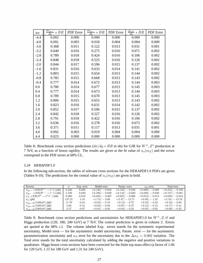
Table 8: Benchmark cross section predictions (dσ/dy ∗ BR in nb) for GJR forW±, Zo production at7 TeV, as a function of boson rapidity. The results are given at the fit value ofαs(mZ) and the errorscorrespond to the PDF errors at 68% CL.

5.24 HERAPDF1.0

In the following sub-section, the tables of relevant cross sections for the HERAPDF1.0 PDFs are given(Tables 9-10). The predictions for the central value ofαs(mZ) are given in bold.

Process σ Exp. error Model error Param. error αS error Total errorσW+ ×BR(W+ → ℓ+ν) [nb] 6.220 0.060 +0.140/ − 0.050 +0.140/ − 0.030 +0.069/ − 0.069 +0.218/ − 0.108σW− ×BR(W− → ℓ−ν) [nb] 4.320 0.030 +0.100/ − 0.030 +0.110/ − 0.020 +0.039/ − 0.039 +0.157/ − 0.061σZ ×BR(Z0 → ℓ+ℓ−) [nb] 0.980 0.010 +0.025/ − 0.007 +0.025/ − 0.006 +0.012/ − 0.012 +0.039/ − 0.018σtt [pb] 147.31 4.10 +1.74/ − 3.09 +2.47/ − 12.71 +0.98/ − 1.24 +5.18/ − 13.76σgg→H(120GeV) [pb] 11.79 0.24 +0.04/ − 0.18 +0.13/ − 0.75 +0.32/ − 0.32 +0.42/ − 0.88σgg→H(180GeV) [pb] 4.86 0.12 +0.02/ − 0.08 +0.07/ − 0.37 +0.12/ − 0.12 +0.17/ − 0.41σgg→H(240GeV) [pb] 2.57 0.07 +0.01/ − 0.05 +0.04/ − 0.22 +0.05/ − 0.05 +0.09/ − 0.25

Table 9: Benchmark cross section predictions and uncertainties for HERAPDF1.0 forW±, Z, tt andHiggs production (120, 180, 240 GeV) at 7 TeV. The central prediction is given in column 2. Errorsare quoted at the 68% c.l. The column labeled Exp. errors stands for the symmetric experimentaluncertainty, Model error — for the asymmetric model uncertainty, Param. error — for the asymmetricparameterization uncertainty andαS error for the uncertainty due to the∆αS = 0.002 variation. TheTotal error stands for the total uncertainty calculated by adding the negative and positive variations inquadrature. Higgs boson cross sections have been correctedfor the finite top mass effect (a factor of 1.06for 120 GeV, 1.15 for 180 GeV and 1.31 for 240 GeV).

27

yWdσW+

dy × BR PDF+αS ErrordσW−

dy × BR PDF+αS ErrordσZ0

dy × BR PDF+αS Error

0.0 0.878 +0.039−0.021 0.771 +0.025

−0.012 0.1634 +0.0074−0.0035

0.4 0.880 +0.040−0.020 0.765 +0.024

−0.012 0.1625 +0.0077−0.0035

0.8 0.885 +0.041−0.019 0.748 +0.025

−0.011 0.1606 +0.0076−0.0033

1.2 0.887 +0.039−0.016 0.720 +0.026

−0.010 0.1568 +0.0077−0.0029

1.6 0.892 +0.039−0.014 0.680 +0.027

−0.010 0.1514 +0.0070−0.0025

2.0 0.893 +0.032−0.015 0.625 +0.024

−0.011 0.1438 +0.0057−0.0030

2.4 0.875 +0.033−0.020 0.548 +0.023

−0.013 0.1313 +0.0056−0.0032

2.8 0.818 +0.047−0.025 0.436 +0.021

−0.015 0.1094 +0.0081−0.0037

3.2 0.658 +0.055−0.029 0.291 +0.025

−0.016 0.0765 +0.0090−0.0033

3.6 0.380 +0.043−0.024 0.135 +0.030

−0.011 0.0337 +0.0066−0.0022

4.0 0.090 +0.014−0.009 0.028 +0.019

−0.005 0.0048 +0.0033−0.0009

4.4 0.002 +0.004−0.001 0.001 +0.004

−0.001 0.0000 +0.0002−0.0000

Table 10: Benchmark cross section predictions (dσ/dy × BR in nb) for HERAPDF1.0 set calculated atαS = 0.1176 as a function of boson rapidity. All sources of error calculated above are included.

5.25 MSTW2008

In the following sub-section, the tables of relevant cross sections for the MSTW2008 PDFs are given(Tables 11-14). The predictions for the central value ofαs(mZ) are given in bold.

αs(mZ) σW+ ∗ BR(W+ → l+ν)[nb] σW− ∗ BR(W− → l−ν)[nb] σZo ∗ BR(Zo → l+l−)[nb]

0.1187 5.897 4.150 0.93360.1194 5.927 4.171 0.93980.1202 5.957 4.190 0.94420.1208 5.982 4.208 0.94790.1214 6.008 4.225 0.95160.1190 5.911 4.160 0.9374

Table 11: Benchmark cross section predictions for MSTW 2008for W±, Z andtt production at 7 TeV,as a function ofαs(mZ). The results for the central value ofαs(mZ) for MSTW 2008 (0.1202) areshown in bold.

αs(mZ) σgg→Higgs(120 GeV )[pb] σgg→Higgs(180 GeV )[pb] σgg→Higgs(240 GeV )[pb] σtt[pb]

0.1187 12.13 5.08 2.74 163.50.1194 12.27 5.14 2.77 165.80.1202 12.41 5.19 2.81 168.10.1208 12.53 5.24 2.83 170.00.1214 12.64 5.29 2.86 171.90.1190 12.18 5.10 2.76 164.4

Table 12: Benchmark cross section predictions for MSTW 2008for gg → Higgs production (massesof 120, 180 and 240 GeV), and fortt production, at 7 TeV, as a function ofαs(mZ). The results for thecentral value ofαs(mZ) for MSTW 2008 (0.1202) are shown in bold. Cross sections havebeen correctedfor the finite top mass effect (a factor of 1.06 for 120 GeV, 1.15 for 180 GeV and 1.31 for 240 GeV).

28

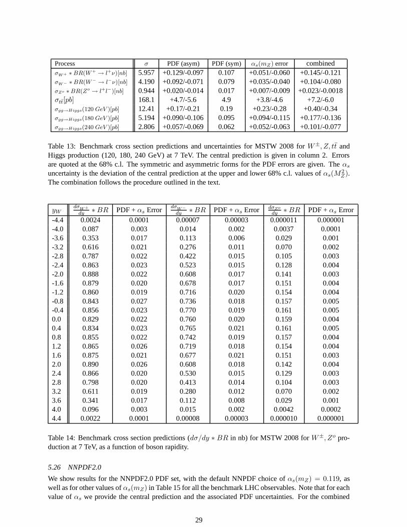
Process σ PDF (asym) PDF (sym) αs(mZ) error combinedσW+ ∗ BR(W + → l+ν)[nb] 5.957 +0.129/-0.097 0.107 +0.051/-0.060 +0.145/-0.121σW− ∗ BR(W− → l−ν)[nb] 4.190 +0.092/-0.071 0.079 +0.035/-0.040 +0.104/-0.080σZo ∗ BR(Zo → l+l−)[nb] 0.944 +0.020/-0.014 0.017 +0.007/-0.009 +0.023/-0.0018σtt[pb] 168.1 +4.7/-5.6 4.9 +3.8/-4.6 +7.2/-6.0σgg→Higgs(120 GeV )[pb] 12.41 +0.17/-0.21 0.19 +0.23/-0.28 +0.40/-0.34σgg→Higgs(180 GeV )[pb] 5.194 +0.090/-0.106 0.095 +0.094/-0.115 +0.177/-0.136σgg→Higgs(240 GeV )[pb] 2.806 +0.057/-0.069 0.062 +0.052/-0.063 +0.101/-0.077

Table 13: Benchmark cross section predictions and uncertainties for MSTW 2008 forW±, Z, tt andHiggs production (120, 180, 240 GeV) at 7 TeV. The central prediction is given in column 2. Errorsare quoted at the 68% c.l. The symmetric and asymmetric formsfor the PDF errors are given. Theαs

uncertainty is the deviation of the central prediction at the upper and lower 68% c.l. values ofαs(M2Z).

The combination follows the procedure outlined in the text.

yWdσW+

dy ∗ BR PDF +αs ErrordσW−

dy ∗ BR PDF +αs Error dσZo

dy ∗ BR PDF +αs Error-4.4 0.0024 0.0001 0.00007 0.00003 0.000011 0.000001-4.0 0.087 0.003 0.014 0.002 0.0037 0.0001-3.6 0.353 0.017 0.113 0.006 0.029 0.001-3.2 0.616 0.021 0.276 0.011 0.070 0.002-2.8 0.787 0.022 0.422 0.015 0.105 0.003-2.4 0.863 0.023 0.523 0.015 0.128 0.004-2.0 0.888 0.022 0.608 0.017 0.141 0.003-1.6 0.879 0.020 0.678 0.017 0.151 0.004-1.2 0.860 0.019 0.716 0.020 0.154 0.004-0.8 0.843 0.027 0.736 0.018 0.157 0.005-0.4 0.856 0.023 0.770 0.019 0.161 0.0050.0 0.829 0.022 0.760 0.020 0.159 0.0040.4 0.834 0.023 0.765 0.021 0.161 0.0050.8 0.855 0.022 0.742 0.019 0.157 0.0041.2 0.865 0.026 0.719 0.018 0.154 0.0041.6 0.875 0.021 0.677 0.021 0.151 0.0032.0 0.890 0.026 0.608 0.018 0.142 0.0042.4 0.866 0.020 0.530 0.015 0.129 0.0032.8 0.798 0.020 0.413 0.014 0.104 0.0033.2 0.611 0.019 0.280 0.012 0.070 0.0023.6 0.341 0.017 0.112 0.008 0.029 0.0014.0 0.096 0.003 0.015 0.002 0.0042 0.00024.4 0.0022 0.0001 0.00008 0.00003 0.000010 0.000001

Table 14: Benchmark cross section predictions (dσ/dy ∗ BR in nb) for MSTW 2008 forW±, Zo pro-duction at 7 TeV, as a function of boson rapidity.

5.26 NNPDF2.0

We show results for the NNPDF2.0 PDF set, with the default NNPDF choice ofαs(mZ) = 0.119, aswell as for other values ofαs(mZ) in Table 15 for all the benchmark LHC observables. Note that for eachvalue ofαs we provide the central prediction and the associated PDF uncertainties. For the combined

29

PDF+αs uncertainty, we assume the benchmark value ofαs (mZ) = 0.1190 ± 0.0012 as a 1–sigmauncertainty.

Next in Table 16 we provide for the same observables the benchmark cross section predictions anduncertainties for the NNPDF2.0 set with the combined PDF andstrong coupling uncertainties at LHC 7TeV. In the last column, the PDF andαs errors are combined using exact error propagation as discussedin Sect. 3.24.

Finally in Table 17 we provide the benchmark cross section predictions for the differential rapiditydistributions (dσ/dy·BR in pb) for NNPDF2.0 forW± andZ0 production at 7 TeV, as a function of theboson rapidity. We provide for each bin in rapidity the combined PDF andαs uncertainty using exacterror propagation.

σ(W+)Br (W+ → l+νl) σ(W−)Br (W− → l+νl)

αs=0.115 5.65 ± 0.13 nb 3.86 ± 0.09 nbαs=0.117 5.73 ± 0.13 nb 3.91 ± 0.08 nbαs=0.119 5.80 ± 0.15 nb 3.97 ± 0.09 nbαs=0.121 5.87 ± 0.13 nb 4.03 ± 0.08 nbαs=0.123 5.98 ± 0.14 nb 4.10 ± 0.10 nb

σ(Z0)Br (Z+ → l+l−) σ(tt)

αs=0.115 886 ± 18 pb 156 ± 5 pbαs=0.117 898 ± 16 pb 162 ± 5 pbαs=0.119 909 ± 19 pb 169 ± 6 pbαs=0.121 921 ± 17 pb 176 ± 6 pbαs=0.123 937 ± 21 pb 182 ± 7 pb

σ(H)(120 GeV) σ(H)(180 GeV) σ(H)(240 GeV)

αs=0.115 11.61 ± 0.25 pb 4.86 ± 0.12 pb 2.69 ± 0.066 pbαs=0.117 11.90 ± 0.19 pb 5.05 ± 0.09 pb 2.75 ± 0.066 pbαs=0.119 12.30± 0.18 pb 5.22 ± 0.10 pb 2.84 ± 0.066 pbαs=0.121 12.66 ± 0.18 pb 5.38 ± 0.09 pb 2.93 ± 0.066 pbαs=0.123 12.92 ± 0.20 pb 5.49 ± 0.10 pb 3.00 ± 0.079 pb

Table 15: Benchmark cross section predictions for NNPDF2.0for W±, Z0, tt and Higgs production at7 TeV, as a function ofαs(mZ). The results for the central value ofαs(mZ) for NNPDF2.0 (0.119)are shown in bold. For each value ofαs(mZ) we provide both the central prediction and the associated1–sigma PDF uncertainties. The Higgs boson cross sections have been corrected for the finite top masseffect (1.06,1.15,1.31) for the three values of the Higgs boson mass.

Process Cross section PDF errors (1–σ) α(mZ) error PDF+αs error

σ(W +)Br(

W + → l+νl

)

[nb] 5.80 0.15 0.04 0.16σ(W +)Br

(

W− → l+νl

)

[nb] 3.97 0.09 0.04 0.10σ(Z0)Br

(

Z+ → l+l−)

[nb] 0.909 0.022 0.007 0.023σ(tt) [pb] 169 6 4 7

σ(H)(120GeV) [pb] 12.30 0.18 0.23 0.29σ(H)(180GeV) [pb] 5.22 0.10 0.10 0.14σ(H)(240GeV) [pb] 2.84 0.066 0.052 0.092

Table 16: Benchmark cross section predictions and uncertainties for NNPDF2.’ forW±, Z0, tt andHiggs production (120, 180, 240 GeV) at LHC 7 TeV. The centralprediction is given in column 2.

30

We provide PDF uncertainties as 1–sigma uncertainties. In the last column, the PDF andαs errors arecombined using exact error propagation as discussed in Sect. 3.24. The Higgs boson cross sections havebeen corrected for the finite top mass effect (1.06,1.15,1.31) for the three values of the Higgs boson mass.

yW/Z dσW+/dy·BR PDF+αs error dσW−/dy·BR PDF+αs error dσZ0/dy·BR PDF+αs error

-4.40 0.0024 0.0003 0.0023 0.00025 0.00001 0.00001-4.00 0.090 0.0048 0.021 0.0021 0.0039 0.00032-3.60 0.352 0.020 0.122 0.007 0.030 0.002-3.20 0.588 0.023 0.279 0.014 0.070 0.0037-2.80 0.771 0.030 0.395 0.016 0.102 0.0042-2.40 0.842 0.030 0.500 0.020 0.124 0.0043-2.00 0.862 0.029 0.569 0.018 0.136 0.0053-1.60 0.851 0.025 0.624 0.020 0.144 0.0038-1.20 0.827 0.040 0.655 0.015 0.147 0.0039-0.80 0.831 0.020 0.687 0.021 0.150 0.0045-0.40 0.819 0.023 0.692 0.017 0.151 0.00340.00 0.815 0.020 0.701 0.019 0.153 0.00490.40 0.836 0.024 0.713 0.016 0.154 0.00310.80 0.820 0.023 0.678 0.016 0.149 0.00461.20 0.840 0.026 0.667 0.017 0.149 0.00441.60 0.858 0.029 0.623 0.020 0.145 0.00392.00 0.860 0.029 0.583 0.024 0.140 0.00512.40 0.861 0.029 0.508 0.019 0.126 0.00462.80 0.771 0.032 0.397 0.017 0.099 0.00473.20 0.598 0.024 0.260 0.013 0.066 0.00373.60 0.338 0.017 0.119 0.007 0.030 0.00254.00 0.076 0.004 0.018 0.0023 0.0044 0.000374.40 0.0016 0.0007 0.0031 0.00031 0.00001 0.00

Table 17: Benchmark cross section predictions (dσ/dy·BR in nb) for NNPDF2.0 forW± andZ0 pro-duction at 7 TeV, as a function of boson rapidity. We provide for each bin in rapidity the combined PDFandαs uncertainty using exact error propagation.

5.3 Comparison of W+,W−, Zo rapidity distributions

NLO predictions for theW+,W− andZ cross sections (along with the PDF uncertainties) are plottedas a function of the boson’s rapidity are plotted in Figure 10using the CTEQ6.6 PDFs.

In the figures below, a comparison is made for the predictionsof theW+,W−, Z0 boson rapiditydistributions for the PDFs discussed in this note. In general, the predictions are in reasonable agreement,but differences can be observed that should be detectable with a reasonably-sized data sample at 7 TeV.

6. Summary

In this interim report, we have tried to provide a snapshot ofour current understanding of PDFs and theassociated experimental and theoretical uncertainties, and of predictions for benchmark cross sectionsat the LHC (7 TeV) and their corresponding uncertainties. This snapshot will be updated as new inputdata/theoretical treatments become available. Many of thePDFs discussed in this note are now not themost recent generation from the respective PDF groups, but we have concentrated on these since theyare in the most common use by the experimental groups.

31

Entries 0

Mean 0

RMS 0

bosony

-4 -3 -2 -1 0 1 2 3 4

/dy*

BR

(nb

)σd

0

0.2

0.4

0.6

0.8

1

Entries 0

Mean 0

RMS 0

/dy*BR (nb)σd/dy*BR (nb)σd/dy*BR (nb)σd

Fig. 10: TheW +, W− andZ cross sections at 7 TeV (along with the PDF uncertainties) asa function of rapidity for the

CTEQ6.6 PDFs. The error bars indicate the PDF+αs uncertainties shown in Table 6.

Entries 0Mean 0RMS 0

W+y

-4 -3 -2 -1 0 1 2 3 4

Rat

io to

CT

EQ

6.6

0.85

0.9

0.95

1

1.05

1.1

1.15Entries 0Mean 0RMS 0

CTEQ6.6

ABKM09

GJR08

HERAPDF1.0

MSTW2008

NNPDF2.0

Fig. 11: TheW + cross section at 7 TeV as a function of rapidity for the PDFs discussed in this note, normalized to the result of

CTEQ6.6. The error bars indicate the PDF(+αs/model/...) uncertainties as defined in the tables providedby each PDF group.

32

Entries 0Mean 0RMS 0

W-y

-3 -2 -1 0 1 2 3

Rat

io to

CT

EQ

6.6

0.85

0.9

0.95

1

1.05

1.1

1.15Entries 0Mean 0RMS 0

CTEQ6.6

ABKM09

GJR08

HERAPDF1.0

MSTW2008

NNPDF2.0

Fig. 12: TheW− cross section at 7 TeV as a function of rapidity for the PDFs discussed in this note, normalized to the result

of MSTW2008. The error bars indicate the PDF(+αs/model/...) uncertainties as defined in the tables providedby each PDF

group.

Entries 0Mean 0RMS 0

Zy

-3 -2 -1 0 1 2 3

Rat

io to

CT

EQ

6.6

0.85

0.9

0.95

1

1.05

1.1

1.15Entries 0Mean 0RMS 0

CTEQ6.6

ABKM09

GJR08

HERAPDF1.0

MSTW2008

NNPDF2.0

Fig. 13: TheZo cross section at 7 TeV as a function of rapidity for the PDFs discussed in this note, normalized to the result

of MSTW2008. The error bars indicate the PDF(+αs/model/...) uncertainties as defined in the tables providedby each PDF

group.

33

References

[1] S. Alekhin, J. Blumlein,P. Jiminez-Delgado,S. Moch and E. Reya, arXiv:1011.6259 [hep-ph].

[2] S. Alekhin, J. Blumlein, S. Klein and S. Moch, Phys. Rev.D 81 (2010) 014032 [arXiv:0908.2766[hep-ph]].

[3] S. Alekhin, J. Blumlein and S. Moch, PoS DIS2010, 021 (2010) arXiv:1007.3657 [hep-ph].

[4] P. M. Nadolskyet al., Phys. Rev. D78 (2008) 013004 [arXiv:0802.0007 [hep-ph]].

[5] H. L. Lai, M. Guzzi, J. Huston, Z. Li, P. M. Nadolsky, J. Pumplin and C. P. Yuan, Phys. Rev. D82,074024 (2010). arXiv:1007.2241 [hep-ph].

[6] M. Gluck, P. Jimenez-Delgado and E. Reya, Eur. Phys. J. C53 (2008) 355 [arXiv:0709.0614 [hep-ph]].

[7] M. Gluck, P. Jimenez-Delgado, E. Reya and C. Schuck, Phys. Lett. B 664, 133 (2008)[arXiv:0801.3618 [hep-ph]].

[8] F. D. Aaron et al. [H1 Collaboration and ZEUS Collaboration], JHEP1001 (2010) 109[arXiv:0911.0884 [hep-ex]].

[9] A. D. Martin, W. J. Stirling, R. S. Thorne and G. Watt, Eur.Phys. J. C63 (2009) 189[arXiv:0901.0002 [hep-ph]].

[10] R. D. Ball, L. Del Debbio, S. Forte, A. Guffanti, J. I. Latorre, J. Rojo and M. Ubiali, Nucl. Phys. B838, 136 (2010) [arXiv:1002.4407 [hep-ph]].

[11] http://indico.cern.ch/conferenceDisplay.py?confId=93790

[12] D. Stumpet al., Phys. Rev. D65 (2001) 014012 [arXiv:hep-ph/0101051].

[13] J. Pumplinet al.,

Phys. Rev. D65 (2001) 014013 [arXiv:hep-ph/0101032].

[14] A. D. Martin, R. G. Roberts, W. J. Stirling and R. S. Thorne, Eur. Phys. J. C28 (2003) 455[arXiv:hep-ph/0211080].

[15] R. D. Ball et al. [NNPDF Collaboration], Nucl. Phys. B809, 1 (2009) [Erratum-ibid. B816, 293(2009)] [arXiv:0808.1231 [hep-ph]].

[16] A. D. Martin, R. G. Roberts, W. J. Stirling and R. S. Thorne, Eur. Phys. J. C39 (2005) 155[arXiv:hep-ph/0411040].

[17] A. D. Martin, W. J. Stirling, R. S. Thorne and G. Watt, Eur. Phys. J. C70, 51 (2010)[arXiv:1007.2624 [hep-ph]].

[18] J. Rojoet al., arXiv:1007.0354 [hep-ph].

[19] F. Demartin, S. Forte, E. Mariani, J. Rojo and A. Vicini,Phys. Rev. D82 (2010) 014002[arXiv:1004.0962 [hep-ph]].

[20] H. L. Lai, J. Huston, Z. Li, P. Nadolsky, J. Pumplin, D. Stump and C. P. Yuan Phys. Rev. D82,054021 (2010) arXiv:1004.4624 [hep-ph].

[21] M. Dittmar et al., arXiv:0901.2504 [hep-ph].

34

[22] S. Bethke, Eur. Phys. J. C64, 689 (2009) [arXiv:0908.1135 [hep-ph]].

[23] A. D. Martin, W. J. Stirling, R. S. Thorne and G. Watt, Eur. Phys. J. C64, 653 (2009)[arXiv:0905.3531 [hep-ph]].

[24] P. M. Nadolsky and Z. Sullivan, inProc. of the APS/DPF/DPB Summer Study on the Future ofParticle Physics (Snowmass 2001)ed. N. Graf,In the Proceedings of APS / DPF / DPB SummerStudy on the Future of Particle Physics (Snowmass 2001), Snowmass, Colorado, 30 Jun - 21 Jul2001, pp P510[arXiv:hep-ph/0110378].

[25] http://mcfm.fnal.gov.

[26] J. Blumlein,S. Riemersma,W. L. van Neervenet al, Nucl.Phys.Proc.Suppl.51C(1996) 97 [hep-ph/9609217].

[27] G. Watt, presented at the PDF4LHC meeting of March 26, 2010 (CERN). Plots fromhttp://projects.hepforge.org/mstwpdf/pdf4lhc/ .

[28] J. R. Andersenet al. [SM and NLO Multileg Working Group], arXiv:1003.1241 [hep-ph].

35