The partition problem: case studies in Bayesian

screening for time-varying model structure

Zesong Liu

Jesse Windle

James G. Scott

The University of Texas at Austin

August 26, 2018

Abstract

This paper presents two case studies of data sets where the main inferential

goal is to characterize time-varying patterns in model structure. Both of these

examples are seen to be general cases of the so-called “partition problem,”

where auxiliary information (in this case, time) defines a partition over sample

space, and where different models hold for each element of the partition.

In the first case study, we identify time-varying graphical structure in the

covariance matrix of asset returns from major European equity indices from

2006–2010. This structure has important implications for quantifying the

notion of financial contagion, a term often mentioned in the context of the

European sovereign debt crisis of this period. In the second case study, we

screen a large database of historical corporate performance in order to identify

specific firms with impressively good (or bad) streaks of performance.

Keywords: Bayesian model selection, contagion, financial crises, graphical

models, multiple testing, tree models

1

arX

iv:1

111.

0617

v1 [

stat

.AP]

2 N

ov 2

011

1 Introduction

Problems of model selection are often thought to be among the most intractable in

modern Bayesian inference. They may involve difficult high-dimensional integrals,

nonconcave solution surfaces, or large discrete spaces that cannot be enumerated.

All of these traits pose notorious computational and conceptual hurdles.

Yet model-choice problems—particularly those related to feature selection, large-

scale simultaneous testing, and inference of topological network structure—are also

some of the most important. As modern data sets have become larger, they have also

become denser—that is, richer with covariates, more deeply layered with underlying

patterns, and indexed in ever more baroque ways (e.g. xijkt, rather than just xij).

It is this complex structure, more than the mere tallying of terabytes, that defines

the new normal in 21st-century statistical science. There is thus a critical need for

Bayesian methodology that addresses the challenges posed by such data sets, which

come with an especially compelling built-in case for sparsity.

The difficulties of model selection are further exacerbated when the structure

of the model is not “merely” unknown, but also changes as a function of auxiliary

information. We call this the partition problem: the auxiliary information defines

an unknown partition over sample space, with different unknown models obtaining

within different elements of the partition. Here are three examples where model

structure plausibly covaries with external predictors.

Subgroup analysis: How can clinicians confront the multiplicity problem inherent

in deciding whether a new cancer drug is effective for a specific subgroup of

patients, even if it fails for the larger population? Here the model is simply a

binary indicator for treatment effectiveness, while the partitions are defined by

diagnostically relevant covariates—for example, age, sex, or smoking status.

No good approaches exist, Bayesian or otherwise, that are capable of system-

atically addressing this problem. The difficulty is that examining all possible

partitions wastes power: many substantively meaningless or nonsensical par-

titions are considered, and must receive prior probability at the expense of the

partitions we care about.

Partitioned variable selection: A patient comes to hospital complaining of a

migraine. The hospital wishes to use the patient’s clinical history to diagnose

whether the migraine may portend a subarchnoid hemorrhage, a catastrophic

form of brain bleed. Such hemorrhages are thought to be etiologically distinct

for children and adults. Thus the age of the patient influences which aspects of

her clinical history (i.e. variables) should be included in the predictive model.

Network drift: A delay-tolerant network (DTN) for communication devices has

2

few instantaneous origin-to-destination paths. Instead, most messages are

passed to their destination via a series of local steps (at close range) from device

to device. In such a setting, it helps to know the underlying social network of

users in the model—that is, who interacts with whom, and how often—in order

to predict the likelihood of success for specific directed transmissions. Thus

the time-varying topological structure of the social network has important

implications for the efficient routing of traffic within the device network.

All three of these problems recall the literature on tree modeling, including [4],

[6], [7], and [11]. Yet to our knowledge no one has studied tree models wherein one

large discrete space (for example, predictors in or out of a linear model) is wrapped

inside another large discrete space (trees).

This poses all the usual computational and modeling difficulties associated with

tree structures, and large discrete spaces more generally. But it also poses a major,

unique challenge. In all existing applications of Bayesian tree models we have en-

countered, the collapsed sampler (whereby node-level parameters are marginalized

away and MCMC moves are made exclusively in tree space) is the computational

tool of choice. But in the partition problem, the bottom level parameter in the

terminal nodes of the tree is itself a model indicator, denoting an element of some

potentially large discrete space. This makes it difficult to compute the marginal

likelihood of a particular tree in closed form, since doing so would involve a sum

with too many terms. The collapsed sampler therefore cannot always be used.

Trees are, of course, just one possible generative model for partitions of a sample

space based on such auxiliary information. Others include species-sampling models,

coalescent models, or urn models (such as those that lie at the heart of Bayesian

nonparametrics). But no matter what partitioning model is entertained, new models

and algorithms are necessary to make inferences and quantify uncertainty for this

very general class of problems.

This chapter presents two case studies of data sets within this class. For both

data sets the auxiliary information is time. In the first case study, we identify time-

varying graphical structure in the covariance of asset returns from major European

equity indices from 2006–2010. This structure has important implications for quan-

tifying the notion of financial contagion, a term often mentioned in the context of the

European sovereign debt crisis of this period. In the second case study, we screen a

large database of historical corporate performance in order to identify specific firms

with impressively good (or bad) streaks of performance.

Our goal in these analyses is not to address all the substantive issues raised by

each data set. Rather, we intend: (1) to present our argument for the existence

of non-trivial dynamic structure in each data set, an argument that can be made

using simple models; (2) to draw parallels between the case studies, both of which

3

exemplify the partition problem quite well; and (3) to identify certain aspects of

each model that must be generalized in future work if these case studies are to

provide a useful template for other data sets.

2 Case study I: financial contagion and dynamic

graphical structure

2.1 Overview

During times of financial crisis, such as the bursting of the US housing bubble in

2008 and the European sovereign-debt crisis in 2010, the co-movement of asset prices

across global markets is hypothesized to diverge from its usual pattern. Many fi-

nancial theorists predict, and many empiricists have documented, changes in market

relationships after these large market shocks. It is important to track these large

shocks and measure their impacts on the global economy so that we can better

understand future market behaviors during times of crisis.

In general, the idea that market relationships change after large shocks is called

contagion [9]. In the literature, there has been a lengthy debate over precise defini-

tion of this term. As a practical matter, we define contagion as significant change

in the pattern of correlation in the residuals from an asset-pricing model during

times of crisis, following in the tradition of previous authors [e.g. 10, 1, 2]. Focusing

primarily on how the relationships between markets change, we want to determine

whether large shocks have significant impact on the subsequent interactions between

markets.

The standard way to study the co-movements and interdependent behavior of

markets is by looking at the covariance matrices of returns across different coun-

tries. In this case study, we explore ways of estimating this covariance structure to

study the change of the market dynamic over time. Normally, when constructing co-

variance matrices, the algorithms applied are computationally identical to repeated

applications of least squares regressions. Instead, we apply the ideas of Bayesian

model selection, using the Bayesian information criterion, or BIC [16], to approxi-

mate the marginal likelihoods of different hypotheses, and a flat prior over model

space.

In applying this method, we uncover many signs of contagion, which manifests

itself as time-varying graphical structural in the covariance matrix of returns. For

example, if we look at the relationship between Italy and Germany, the traditionally

positive correlation between the countries changes sign during the sovereign debt

crisis. This provides just one example of the evidence for contagion discovered in

4

these investigations.

2.2 Contagion in factor asset-pricing models

The sovereign debt crisis started when Greece became in danger of defaulting on

its debt. For years, Greece had been a rapidly growing economy with many foreign

investors. This strong economy was able to withstand large government deficits that

Greece had during that time. But after the worldwide 2008 financial crisis hit, two

of the country’s largest industries, tourism and shopping, were badly affected. This

downturn caused panic in the Greek economy. Although Greece was not the only

country that confronted debt problems, its debt-to-GDP ratio was judged excessively

high by markets and ratings agencies, reaching 120% in 2010. Moreover, one of the

major fears that arose during this period was that investors would lose faith in other

similary situated Euro-zone economies, which could cause something similar to a run

on a bank.

One of the major events in this episode occurred on May 9, 2010. On that day

the 27 member states of the EU agreed to create the European Financial Stability

Facility, a legal instrument aimed at preserving financial stability in Europe by

providing financial assistance to states in need. This legislation was upsetting to

countries with large healthy economies such as Germany, whose electorate focused

on the negative effects of the bailout. In light of these developments, not only do

we want to show that the pattern of asset-price correlation changed, but we also

want to make sense of these changes by linking them to the news headlines about

bailouts.

Our raw data are daily market returns from equity indices corresponding to nine

large European economies—Germany, the UK, Italy, Spain, France, Switzerland,

Sweden, Belgium, and the Netherlands—from December 2005 to October 2010. We

do not include Greece because of its small size relative to the other economies of

Europe, but we do include the Euro–Dollar exchange rate as a tenth column in the

data set.

By our definition of contagion, we need to examine the residuals of the returns

within the context of an asset-pricing model. Specifically, we use a four-factor model

where

E(yit | EU,US) = βUSi xUSt + βEUi xEUt + γUSi δUSt + γEUi δEUt ,

where yit is the daily excess return on index i; xUSt is the daily excess return on

a value-weighted portfolio of all US equities; xEUt is the daily excess return on the

EU-wide index of Morgan Stanley Capital International; δUSt is the volatility shock

to the US market; and δEUt is the excess volatility shock to the European market.

The excess shock is defined as the residual after regressing the EU volatility shock

5

upon the US volatility shock. This is necessary to avoid marked collinearity, since

the US volatility shock strongly predicts the EU volatility shock. These volatility

factors are calculated using the particle-learning method from [14], not described

here.

In this model, the loadings βUSi and βEUi measure the usual betas relative to

the US and Europe-wide equity markets. Thus we have controlled for regional

and global market integration via an international CAPM-style model [2]. The

loadings γUSi and γEUi , meanwhile, measure country-level dependence upon global

and regional volatility risk factors. As shown in Polson and Scott [14], these loadings

can be interpreted in the context of a joint model that postulates correlation between

shocks to aggregate market volatility and shocks to contemporaneous country-level

returns.

2.3 A graphical model for the residuals

The above model can be fit using ordinary least squares, leading to an estimate of

all model parameters along with a set of residuals εit for all indices. We now turn

to the problem of imposing graphical restrictions on the covariance matrix of these

residuals.

A Gaussian graphical model defines a set of pairwise conditional-independence

relationships on a p-dimensional zero-mean, normally distributed random vector

(here denoted x). The unknown covariance matrix Σ is restricted by its Markov

properties; given Ω = Σ−1, elements xi and xj of the vector x are conditionally

independent, given their neighbors, if and only if Ωij = 0. If G = (V,E) is an

undirected graph whose nodes represent the individual components of the vector x,

then Ωij = 0 for all pairs (i, j) /∈ E. The covariance matrix Σ is in M+(G), the set

of all symmetric positive-definite matrices having elements in Σ−1 set to zero for all

(i, j) /∈ E.

We construct a graph by selecting a sparse regression model for each country’s

residuals in terms of all the other countries, as in [8] and [20]. We then cobble

together the resulting set of conditional relationships into a graph to yield a valid

joint distribution. Each sparse regression model is selected by enumerating all 29

possible models, and choosing the one that minimizes the BIC. This leads to a

potentially sparse model for E(εit | εj,t, j 6= i).

In this manner, an adjacency matrix can be constructed for the residuals from

the four-factor model. The (i, j) element of the adjacency matrix is equal to 1 if

the residuals for countries i and j both appear in each other’s conditional regression

models, and is equal to 0 otherwise. One may also assemble the pattern of coeffi-

cients from these sparse regressions to reconstruct the covariance matrix for all the

6

residuals, denoted Σ.

We actually look at adjacency matrices and covariance matrices on a rolling

basis, since we believe that there are changes in Σ over time. Each window involves

a separate set of regressions for a period of 150 trading days, which is thirty weeks

of trading, or about 7 months. We shift the window in 5 day increments, thereby

spanning the whole five-year time period in our study. For each 150-day window,

we refit the estimate for Σt using the entire graphical-model selection procedure.

For the sake of comparison, we also include the estimates of Σt using OLS, ridge

regression, and lasso regression.

2.4 Results

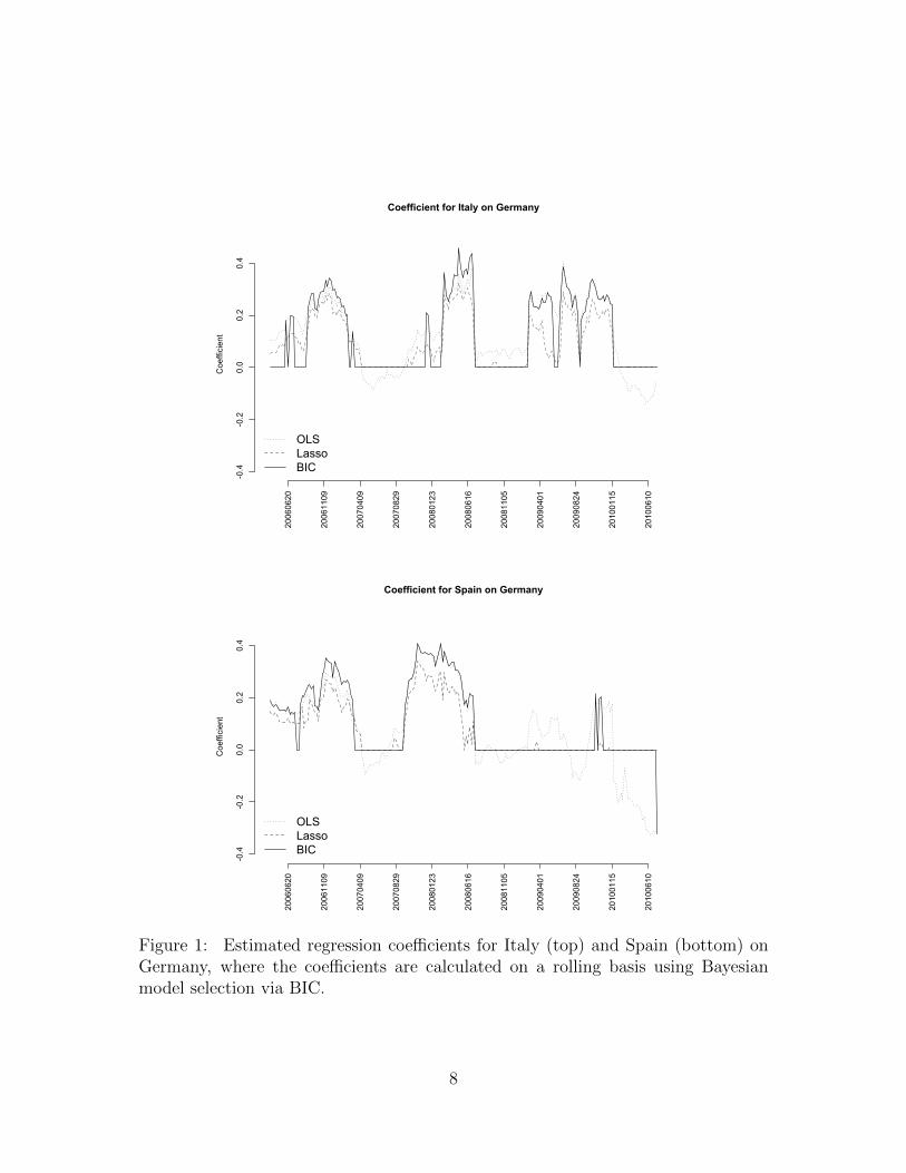
From Figure 1, which depicts the rolling estimates of the Italy–Germany and Spain–

Germany regression coefficients, it is clear that there are nonrandom patterns that

remain in the residuals. If the factor model fully explained the co-movements in

the European market, we would expect the residuals to have no covariance and look

like noise. We would also expect that the Bayesian variable-selection procedure

would give regression coefficients of 0. To be sure, the data support the hypothesis

that specific elements of the precision matrix Ωt = Σ−1t are zero over certain time

periods. An example of this is the ITA-DEU coefficient during much of 2008. Yet

it is patently not the case that all such elements are zero for all time periods: the

standard significance test of an empty graph is summarily rejected (p < 10−6) at all

time points. For details of this test, see [13] and Proposition 1 of [5].

There are several explanations for the observed correlation between the residu-

als. First, it is highly probable that the factor models are imperfect. Regressing

only on the market returns and market volatility, the four factor model involves a

substantial simplification of reality. For example, during the sovereign debt crisis,

we could reasonably add an explanatory variable that takes into account the change

in likelihood of a bailout. Second, even if we imagine that the four-factor model

is the true model for this system of markets, we only have proxies for both the

global and local returns and volatility. Specifically, using the US market return as a

proxy for the world market return is a reasonable estimate, but is far from perfect.

Moreover, the factors that measure market volatility are at best a measure of the

average market volatility over a short time span. This could potentially distort the

residuals, since we cannot observe volatility spikes on a more granular scale. Most

likely, the correlations in the residuals stems from some mixture of these two effects.

The same conclusion about significant residual correlation is also borne out by

examining the time-varying topology of the graph itself. While it is difficult to

visualize the time-varying nature of the network’s structure in its entirety, we can

7

Coefficient for Italy on GermanyCoefficient

-0.4

-0.2

0.0

0.2

0.4

20060620

20061109

20070409

20070829

20080123

20080616

20081105

20090401

20090824

20100115

20100610

OLSLassoBIC

Coefficient for Spain on Germany

Coefficient

-0.4

-0.2

0.0

0.2

0.4

20060620

20061109

20070409

20070829

20080123

20080616

20081105

20090401

20090824

20100115

20100610

OLSLassoBIC

Figure 1: Estimated regression coefficients for Italy (top) and Spain (bottom) onGermany, where the coefficients are calculated on a rolling basis using Bayesianmodel selection via BIC.

8

Degree of UK in GraphCoefficient

02

46

810

20060620

20061109

20070409

20070829

20080123

20080616

20081105

20090401

20090824

20100115

20100610

LassoBIC

Degree of Sweden in Graph

Coefficient

02

46

810

20060620

20061109

20070409

20070829

20080123

20080616

20081105

20090401

20090824

20100115

20100610

LassoBIC

Figure 2: Estimated adjacency degree in the time-varying graph of residuals for theUK (top) and Sweden (bottom). There seems to be clear evidence of time-varyingtopological structure in the graph.

9

look at quantities such as how the adjacency of a specific node in the graph—that

is, how many neighbors it has—changes over time. Figure 2 shows the estimated

adjaceny degrees for Sweden and the UK, two non-Euro countries. Again we see

that the factor model is not perfect, as the residuals still exhibit correlation. On the

other hand, we see that the degree of each vertex is not 9 at every time point. This

means that shrinkage is often useful: it is clear that estimating p(p− 1)/2 separate

correlation parameters is a poor use of the data, and will lead to estimators with

unnecessarily high variance. We can almost certainly reduce the required number

of parameters while still obtaining a good estimate. This illustrates the utility of

the graphical modeling approach.

Finally, the relationship between the Spain and Germany residuals is easily in-

terpretable in terms of the underlying economic picture. In the summer of 2010,

there is an apparent divergence from the historical norm, precisely coinciding with

the Greek sovereign-debt crisis and associated bailout. The historically aberrant

negative correlations between the residuals from Germany and the southern coun-

tries suggests that markets reacted very differently in these two countries to news

of the period. A useful comparison is with the period of September and October

2008, when the global financial crisis associated with the bursting of the housing

bubble was at its peak. These were global rather than EU-centric events, and no

such divergence was observed involving the German-market residuals.

Our approach provides initial evidence for contagion effects, but has some impor-

tant limitations. In particular, we have estimated time-varying graphical structure

using a moving-window variable selection approach, which does not explicitly in-

volve a dynamic model over graph space. Some authors have made initial efforts in

studying dynamic graphs [e.g. 21, 22], but much further work remains to be done to

operationalize the notion of contagion within this framework. The issue is that we

expect contagion to be associated with a sharp change in the underlying graphical

structure of the residual covariance matrix, as opposed to the locally drifting models

considered by these other authors. Such sharp changes are likely obscured by our

rolling-regression approach, in that only about 3% of the data changes in each new

window.

10

3 Case study II: simultaneous change-point screen-

ing and corporate out-performance

3.1 Overview

In this case study, we compare publicly traded firms against their peer groups us-

ing a standard accounting metric known as ROA, or return on assets. The data

set comprises 645,456 company-year records from 53,038 companies in 93 different

countries, spanning the years 1966-2008.

Just as in the previous example, we will attempt to uncover substantively mean-

ingful changes over time in the underlying model for each time series. Let yit denote

the benchmarked ROA observation for company i at time t; let yi denote the whole

vector of observations for company i observed at times ti = (t1, ..., tni); and let Y

denote the set of yi for all i. We say the observations have been “benchmarked” to

indicate that they have undergone a pre-processing step that removes the effects of

a firm’s size, industry, and capital structure. For details, see [18].

The goal is to categorize each time series i as either signal or non-signal, both

to be defined shortly. The model we consider takes the general form

yi = fi + εi, εi ∼ Noise (1)

fi ∼ ω · Signal + (1− ω) · Null (2)

where Signal is the distribution describing the signal and Null is the distribution

describing the non-signal. In this case, “noise” should not be conflated with actual

measurement error. Instead, it represents short-term fluctuations in performance

that are not indicative of any longer-term trends, and are thus not of particular

relevance for understanding systematic out-performance.

We can rephrase this model as

yi = fi + εi, εi ∼ Noise

fi ∼ Fγi , F1 = Signal, F0 = Null (3)

γi ∼ Bernoulli(ω)

which provides us with the auxiliary variable γi that determines whether a time

series i is either signal or noise. Thus the posterior distribution p(γi = 1|Y) is a

measure of how likely time series i is signal. One can sort the data points from most

probably to least probably signal by simply ranking p(γi = 1|Y). Importantly, these

posterior probabilities will contain an automatic penalty for data dredging: as more

unimpressive firms are thrown into the cohort, the posterior distribution for ω will

11

favor increasingly smaller values, meaning that all observations have to work harder

to overcome the prior bias in favor of the null [see, e.g., 19, 3].

Suppose, for example, that fi = 0 corresponds to the average performance of a

company’s peer group, and that we want deviations from zero to capture long-range

fluctuations in yi from this peer-group average—that is, changes in a company’s

fortunes or long-run trends that unfold over many years. Several previous authors

have proposed methodology for the multiple-testing problem that arises in deciding

whether fi = 0 for all firms simultaneously [17, 12, 15]. The origin of such a testing

problem lies in the so-called “corporate success study,” very popular in the business

world: begin with a population of firms, identify the successful ones, and then look

for reproducible behaviors or business practices that explain their success.

The hypothesis that fi = 0, then, implies that a firm is no better, or worse, than

its peer group over time. One way to test this hypothesis is by placing a Gaussian-

process prior on those fi’s that differ from zero. Suppose, for example, we have an

i.i.d. error structure and some common prior inclusion probability:

yi = fi + εi, εi ∼ N(0, σ2I)

fi ∼ Fγi , F1 = N(0, σ2K(ti)), F0 = δ0

γi ∼ Bernoulli(ω)

where K(t) is the matrix produced by a covariance kernel k(·, ·), evaluated at the

observed times t = (t1, ..., tM)′. The (i, j) entry of K is:

Ki,j = k(ti, tj).

Typically the covariance function will itself have hyperparameters that must be

either fixed or estimated. A natural choice here is the squared-exponential kernel:

k(ti, tj) = κ1 exp− (ti − tj)2

2κ

+ κ3δti,tj

where δti,tj is the Kronecker delta function. If the three κ hyperparameters are

fixed, then this is just a special case of a conjugate multivariate Gaussian model,

and the computation of the posterior model probabilities p(γi = 1|Y) may proceed

by Gibbs sampling. As shown in [17], this basic idea may be generalized to more

complicated models involving autoregressive error structure and Dirichlet-process

priors on nonzero trajectories.

12

3.2 Detecting regime changes

One shortcoming of this strategy is that fi is assumed to be either globally zero

or globally nonzero. The partition problem is different, and captures an important

aspect of reality ignored by the model above: the signal of interest may not involve

consistent performance, but rather a precipitous rise or fall in the fortunes of a

company.

We therefore consider the possibility that each firm’s history may, though not

necessarily, be divided into two epochs. The separation of these epochs corresponds

to some sort of significant schism in performance between time periods. For instance,

a positive jump might arise by virtue or a drug patent or the tenure of an especially

effective leader–someone like Steve Jobs of Apple, or Jack Welch of General Electric.

There may also be periods of inferior performance when the jump is negative.

We therefore adapt model (3) in the following way. With each firm, we associate

not a binary indicator of “signal” or “noise”, but rather a multinomial indicator

for the location in time of a major shift in performance. We then index all further

parameters in the model by this multinomial indicator:

yi = fi + εi, εi ∼ Noise

fi ∼ Fγi (4)

γi ∼ Multinomial(ω) ,

with the convention that γi = 0 denotes the no-split case where fi is globally zero,

and γi = n the no-split case where fi is globally non-zero.

This differs from the traditional changepoint-detection problem in two respects:

we are data-poor in the time direction, but data-rich in the cross-section. Indeed,

this case study is the mirror image of the previous one, where the number of time

series was moderate the number of observations per times series was large. This fact

requires us to consider models that are simpler in the time domain, but also allows

us to borrow cross-sectional information across firms for the purpose of estimat-

ing shared model parameters. This is particularly important for the multinomial

parameter ω, which lives on the (n + 1)-dimensional simplex, and descibes the

population-level distribution of changepoints.

There are many potential choices for Fk and Noise. We instance, we could choose

Fk = N(0, Ck) and Noise = N(0,Σ)

where Σ describes the covariance structure of the noise and Ck describes a split in

epochs at time k (again recalling the convention that C0 is degenerate at zero and

that Cn corresponds to no split at all). Of course, we need not limit ourselves to this

13

interpretation, and may intead choose a collection of Ck that embodies some other

substantive meaning. For instance, we could consider the collection Ci,k where C1,k

corresponds to a small jump at time k and C2,k corresponds to a large jump at time k.

We could also generalize to multiple regime changes per firm. For now, however, we

consider the simpler case where there can be at most one shift, and where all shifts

are exchangeable. Recall that we intend such an intentionally oversimplified model

to be useful for high-dimensional screening, not nuanced modeling of an individual

firm’s history.

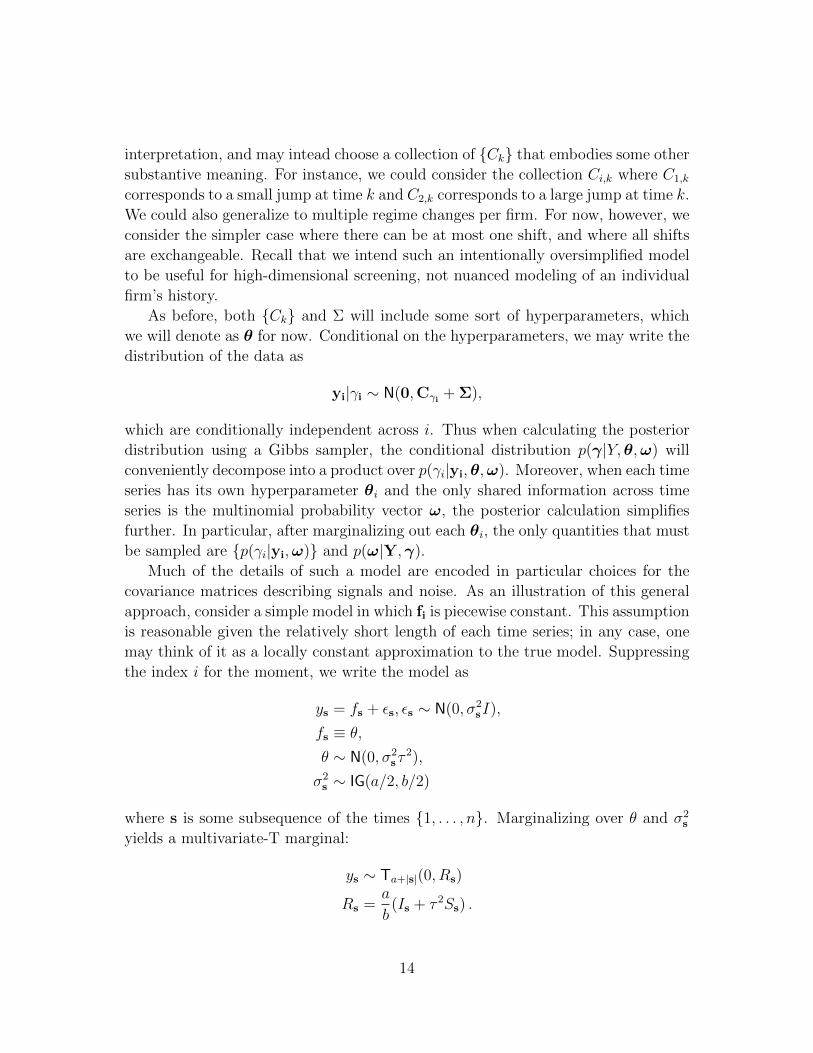
As before, both Ck and Σ will include some sort of hyperparameters, which

we will denote as θ for now. Conditional on the hyperparameters, we may write the

distribution of the data as

yi|γi ∼ N(0,Cγi + Σ),

which are conditionally independent across i. Thus when calculating the posterior

distribution using a Gibbs sampler, the conditional distribution p(γ|Y,θ,ω) will

conveniently decompose into a product over p(γi|yi,θ,ω). Moreover, when each time

series has its own hyperparameter θi and the only shared information across time

series is the multinomial probability vector ω, the posterior calculation simplifies

further. In particular, after marginalizing out each θi, the only quantities that must

be sampled are p(γi|yi,ω) and p(ω|Y,γ).

Much of the details of such a model are encoded in particular choices for the

covariance matrices describing signals and noise. As an illustration of this general

approach, consider a simple model in which fi is piecewise constant. This assumption

is reasonable given the relatively short length of each time series; in any case, one

may think of it as a locally constant approximation to the true model. Suppressing

the index i for the moment, we write the model as

ys = fs + εs, εs ∼ N(0, σ2sI),

fs ≡ θ,

θ ∼ N(0, σ2sτ

2),

σ2s ∼ IG(a/2, b/2)

where s is some subsequence of the times 1, . . . , n. Marginalizing over θ and σ2s

yields a multivariate-T marginal:

ys ∼ Ta+|s|(0, Rs)

Rs =a

b(Is + τ 2Ss) .

14

If we know θ = 0, or in other words that θ ∼ δ0, then Rs = (a/b)Is. Notice that this

formulation automatically handles missing data, since one can simply exclude those

times from s.

This can be phrased in terms of model (4) by letting Sk = 1k1′k be the k × k

matrix of ones, and defining

Fk = N(0, τCk) ,

where

Ck|σ2ij =

[σ2i1Sk 0

0 σ2i2Sn−k

]for k = 1, · · · , n− 1,

Fn = N(0, σ2i τSn), and F0 = δ0 (that is Cn = σ2

i Sn and C0 = 0). Furthermore, we

define the prior over the residuals so that it, too, depends on the index γi:

Noise = Eγi = N(0,Σγi)

where Σk|σ2ij = σ2

1iI for k = 0 and n, and where

Σk|σ2ij =

[σ2i1I 0

0 σ2i2I

]for k = 1, . . . , n− 1 ,

Finally, for p(ω) we assume a conjugate Dirichlet prior (details below).

This simple model has many advantages: it is analytically tractable; it handles

missing data easily; it allows for the possibility of a sharp break between epochs;

and it allows for preprocessing of all marginal likelihoods, which saves time in the

Gibbs sampler. To see this, observe that the conditional posterior distribution for

γ is

p(γ|Y,ω) ∝∏i

p(yi|γi,ω)p(γi|ω)

so we can sample each p(γi|yi,ω) independently. In particular,

p(γi = k|Y,ω) ∝ p(yi|γi = k)p(γi = k|ω).

Let `k be the observation times which are less than or equal to k and rk be the

observation times which are greater than k, both of which depend upon i. When

k > 0,

p(γi = k|Y,ω) ∝ Ta+|`k|(yi(`k); 0,R`k) · Ta+|rk|(yi(rk); 0,Rrk) · p(γi = k|ω)

15

with the convention that rk = ∅ if k = n. When k = 0,

p(γi = k|Y,ω) ∝ Ta+|`k|(yi(ti); 0,a

bIti) p(γi = k|ω)

All of the T densities can be computed beforehand for each i and k, and the con-

ditional posterior distribution of γi may be calculated directly over the simplex

0, . . . , n.When implementing this model, we restrict our data set to those firms which

have at least 20 observations, leaving us with 6067 data points. Including firms with

fewer data points would eliminate the possibility of survivorship bias, but would

likely result in a significant decrease in power for the firms with longer histories,

because of shared dependence of all firms on p(ω | Y).

Following the discussion above, the posterior distribution was simulated using a

Gibbs sampler with 3000 steps. We set τ 2 = 10.0 and chose the prior distributions

as follows: IG(2.0/2, 2.0/2) for all noise variance parameters; and ω ∼ Dirichlet(α)

with α0 = 0.8, αn = 0.1, and αi = 0.1/(n − 1) for i = 1, . . . , n − 1. This reflects

the belief, borne out by prior studies, that most firms do not systematically over-

or under-perform their peer groups over time. The choice of τ 2 = 10 will result

in increased power for detecting major shifts in performance, but also a significant

Occam’s-razor penalty against small shifts.

One must be careful in interpreting the posterior distribution p(γ|Y) that arises

from this model. For instance, it may not be meaningful to categorize time series i

in terms of the single time point j that maximizes p(γi = j|Y), since it is entirely

possible that p(γi = j|Y) is of comparable magnitude for a range of different values

of j. This would suggest either no split, or a split that cannot be localized very

precisely. In such cases, it may be more appropriate to look at firms where the

largest entry p(γi | Y) is sufficiently large. This would be strong evidence that there

is a split at time j for time series i.

Figure 3 provides intuition for the various scenarios we might encounter: the

posterior of γi may strongly favor γi = 0 or γi = n, in which case no split occurs; it

may show evidence of a split, but at an ambiguous time; it may show strong, but

not decisive evidence of a split; or it may be flat, which does not tell us anything.

The ideal case for interpretation, of course, would involve strong evidence of a split

at a particular time, as seen in the last pane of Figure 3.

In examining these plots, it appears that the posterior mode

PM(γi) = max0<j<n

p(γi = j|Y)

provides a good measure of a change in epochs as long as we chose a sufficiently high

16

cutoff, such as requiring that the maximum satisfy max0<j<nγi = j|Y > 0.95. To

check that this is reasonable, we plot the histogram of PM(γi) in Figure 4. Of the

3033 firms, only 58 have a value greater than or equal to 0.95. The largest twenty

posterior modes were used to select the time series in Figure 5.

4 Discussion

In each of these two case studies, we have confronted a similar problem: time-varying

model uncertainty for each of many different time series observed in parallel. In the

first case, the model was a graph, encoding conditional independence relationships

about residuals from country-level returns during the European sovereign debt crisis.

In the second case, the model was an indicator of whether a firm’s historical ROA

trajectory was significantly different from its peer-group average. These were seen to

be examples of a general class of problems wherein the model changes as a function

of auxiliary information.

The models we have entertained are based upon fairly standard tools, and were

chosen specifically to avoid the difficulties associated with the most general form

of partitioning that were mentioned in the introduction. They are thus more ap-

propriate for first-pass screening than for detailed analysis. Nonetheless, even these

simple models were sufficient to support the general thrust of our argument: that

each data set exhibited non-trivial dynamic model structure. In each case, further

work is clearly needed to build upon the limited, broad-brush conclusions that can

be reached within the context of these simple models.

17

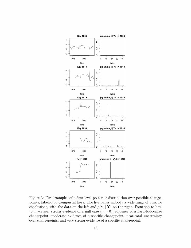
Figure 3: Five examples of a firm-level posterior distribution over possible change-points, labeled by Compustat keys. The five panes embody a wide range of possibleconclusions, with the data on the left and p(γi | Y) on the right. From top to bot-tom, we see: strong evidence of a null case (γ = 0); evidence of a hard-to-localizechangepoint; moderate evidence of a specific changepoint; near-total uncertaintyover changepoints; and very strong evidence of a specific changepoint.

18

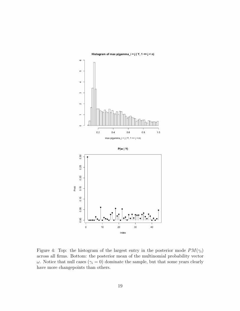
Figure 4: Top: the histogram of the largest entry in the posterior mode PM(γi)across all firms. Bottom: the posterior mean of the multinomial probability vectorω. Notice that null cases (γi = 0) dominate the sample, but that some years clearlyhave more changepoints than others.

19

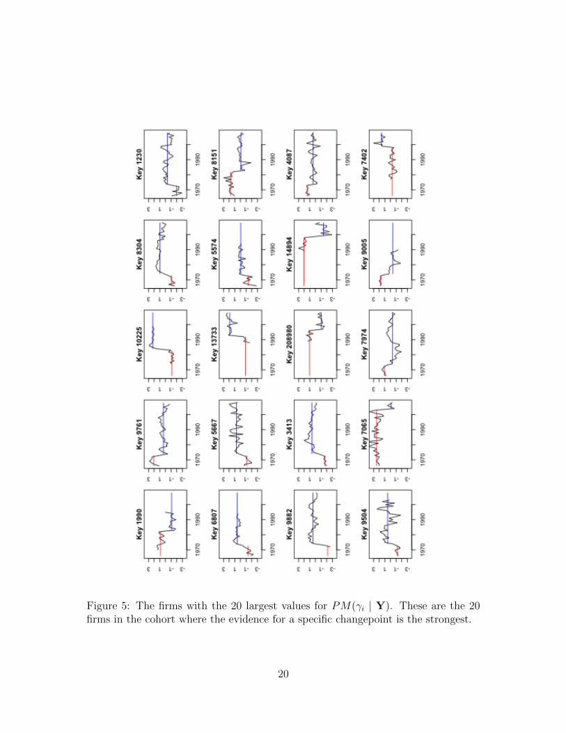
Figure 5: The firms with the 20 largest values for PM(γi | Y). These are the 20firms in the cohort where the evidence for a specific changepoint is the strongest.

20

References

[1] K. Bae, G. Karolyi, and R. Stulz. A new approach to measuring financial contagion.Review of Financial Studies, 16(3):717–63, 2003.

[2] G. Bekaert, C. Harvey, and A. Ng. Market integration and contagion. Journal ofBusiness, 78(1):39–69, 2005.

[3] M. Bogdan, A. Chakrabarti, F. Frommlet, and J. K. Ghosh. Asymptotic Bayes-optimality under sparsity of some multiple testing procedures. The Annals of Statis-tics, 39(3):1551–79, 2011.

[4] L. Breiman, J. H. Friedman, R. A. Olshen, and C. J. Stone. Classification andRegression Trees. Chapman and Hall/CRC, 1984.

[5] C. M. Carvalho and J. G. Scott. Objective Bayesian model selection in Gaussiangraphical models. Biometrika, 96(3):497–512, 2009.

[6] H. A. Chipman, E. I. George, and R. E. McCulloch. Bayesian CART model search.Journal of the American Statistical Association, 93(443):935–48, 1998.

[7] D. G. Denison, B. K. Mallick, and A. F. Smith. A Bayesian CART algorithm.Biometrika, 85(2):363–77, 1998.

[8] A. Dobra, B. Jones, C. Hans, J. Nevins, and M. West. Sparse graphical models forexploring gene expression data. Journal of Multivariate Analysis, 90:196–212, 2004.

[9] R. Dornbusch, Y. C. Park, and S. Claessens. Contagion: Understanding how itspreads. The World Bank Research Observer, 15(2):177–97, 2000.

[10] K. J. Forbes and R. Rigobon. No contagion, only interdependence: Measuring stockmarket comovements. The Journal of Finance, 57:2223–61, 2002.

[11] R. Gramacy and H. K. Lee. Bayesian treed Gaussian process models with an appli-cation to computer modeling. Journal of the American Statistical Association, 103(483):1119–30, 2008.

[12] A. D. Henderson, M. E. Raynor, and M. Ahmed. How long must a firm be great torule out luck? benchmarking sustained superior performance without being fooledby randomness. In The Academy of Management Proceedings, 2009.

[13] S. L. Lauritzen. Graphical Models. Clarendon Press, Oxford, 1996.

[14] N. G. Polson and J. G. Scott. Explosive volatility: a model of financial contagion.Technical report, University of Texas at Austin, 2011.

21

[15] N. G. Polson and J. G. Scott. Good, great, or lucky? screening for firms withsustained superior performance using heavy-tailed priors. The Annals of AppliedStatistics, 2012 (to appear).

[16] G. Schwarz. Estimating the dimension of a model. Annals of Statistics, 6(2):461–464,1978.

[17] J. G. Scott. Nonparametric Bayesian multiple testing for longitudinal performancestratification. The Annals of Applied Statistics, 3(4):1655–74, 2009.

[18] J. G. Scott. Benchmarking historical corporate performance. Technical report, Uni-versity of Texas at Austin, http://arxiv.org/abs/0911.1768, 2010.

[19] J. G. Scott and J. O. Berger. An exploration of aspects of Bayesian multiple testing.Journal of Statistical Planning and Inference, 136(7):2144–2162, 2006.

[20] J. G. Scott and C. M. Carvalho. Feature-inclusion stochastic search for Gaussiangraphical models. Journal of Computational and Graphical Statistics, 17(790–808),2008.

[21] M. Taddy, R. B. Gramacy, and N. G. Polson. Dynamic trees for learning and design.Journal of the American Statistical Association, 106(493):109–23, 2011.

[22] H. Wang, C. Reeson, and C. M. Carvalho. Dynamic financial index models: Modelingconditional dependencies via graphs. Bayesian Analysis, 2011.

22