Clemson UniversityTigerPrints

All Theses Theses

8-2015

THE PARTIALLY RECHARGEABLEELECTRIC VEHICLE ROUTING PROBLEMWITH TIME WINDOWS ANDCAPACITATED CHARGING STATIONSNavid Matin MoghaddamClemson University, nmatinm@clemson.edu

Follow this and additional works at: https://tigerprints.clemson.edu/all_theses

Part of the Engineering Commons

This Thesis is brought to you for free and open access by the Theses at TigerPrints. It has been accepted for inclusion in All Theses by an authorizedadministrator of TigerPrints. For more information, please contact kokeefe@clemson.edu.

Recommended CitationMatin Moghaddam, Navid, "THE PARTIALLY RECHARGEABLE ELECTRIC VEHICLE ROUTING PROBLEM WITH TIMEWINDOWS AND CAPACITATED CHARGING STATIONS" (2015). All Theses. 2205.https://tigerprints.clemson.edu/all_theses/2205

THE PARTIALLY RECHARGEABLE ELECTRIC VEHICLE ROUTING PROBLEM

WITH TIME WINDOWS AND CAPACITATED CHARGING STATIONS

A Thesis

Presented to

the Graduate School of

Clemson University

In Partial Fulfillment

of the Requirements for the Degree

Master of Science

Industrial Engineering

by

Navid Matin Moghaddam

August 2015

Accepted by:

Dr. Scott J Mason, Committee Chair

Dr. Amin Khademi

Dr. Yongxi Huang

ii

ABSTRACT

Electric vehicles are potentially beneficial for both the environment and an

organization’s bottom line. These benefits include, but are not limited to, reduced fuel

costs, government tax incentives, reduced greenhouse gas emissions, and the ability to

promote a company’s “green” image. In order to decide whether or not to convert or

purchase electric trucks and install charging facilities, decision makers need to consider

many factors including onboard battery capacity, delivery or service assignments,

scheduling and routes, as well as weather and traffic conditions in a well-defined

modeling framework. We develop a model to solve the partially rechargeable electric

vehicle routing problem with time windows and capacitated charging stations. Given

destination data and vehicle properties, our model determines the optimal number of

vehicles or charging stations needed to meet the network’s requirements. Analyzing the

model shows the relationships between vehicle range, battery recharge time, and fleet

size.

iii

TABLE OF CONTENTS

Page

TITLE PAGE .................................................................................................................... i

ABSTRACT ..................................................................................................................... ii

LIST OF TABLES .......................................................................................................... iv

LIST OF FIGURES ......................................................................................................... v

CHAPTER

I. INTRODUCTION ......................................................................................... 1

II. LITERATURE REVIEW .............................................................................. 3

III. PROBLEM DESCRIPTION ........................................................................ 11

IV. MATHEMATICAL MODEL ...................................................................... 12

Notation.................................................................................................. 12

Model Formulation ................................................................................ 13

V. MODEL VALIDATION ............................................................................. 18

VI. MODEL PARAMETER ESTIMATION ..................................................... 24

VII. EXPERIMENTAL STUDY......................................................................... 27

Experimental Plan .................................................................................. 27

Experimental Results and Analysis ....................................................... 30

CONCLUSIONS AND FUTURE WORK .................................................................... 34

REFERENCES .............................................................................................................. 35

iv

LIST OF TABLES

Table Page

1 Input Data for Example Problem ................................................................. 19

2 Comparison between Results ....................................................................... 23

3 Experimental Design Parameters ................................................................. 27

4 Experimental Time Window Data ............................................................... 29

5 Experimental Results for Time Windows Set R1 ........................................ 31

6 Experimental Results for Time Windows Set R2 ........................................ 31

7 Relative Optimality Gap for Time Windows Set R1 ................................... 32

8 Relative Optimality Gap for Time Windows Set R2 ................................... 32

9 Percentage of Instances Able to Use Only One Electric Vehicle ................ 33

v

LIST OF FIGURES

Figure Page

1 Data for Test Instance .................................................................................. 19

2 Results for Test Instance (objective is to minimize number of vehicles) .... 21

3 Results for Test Instance (objective is to minimize number of stations) ..... 22

4 Instance Representation ............................................................................... 28

1

1. INTRODUCTION

The Vehicle Routing Problem (VRP) is concerned with finding effective routes

for a set of vehicles. These vehicles must visit a number of customers in different

geographical locations. Each customer has a demand and the objective typically

associated with a VRP is to satisfy this demand with minimum cost of vehicle travel from

a depot.

Electric vehicles, especially battery-powered electric trucks, carry potential long-

term economic and environmental benefits for reduced fuel cost, government tax

incentives, reduced greenhouse gas emissions, and the ability to promote a company’s

“green” image. There are many benefits of electrification that companies can take

advantage of today. However, limited travel range (“range anxiety”) and intense capital

investment have hindered progress. The typical electric truck’s 50-100 mile travel range

makes electric trucks particularly suitable for urban trips, given well-calibrated routing

plans. The investments to convert or purchase electric trucks and install charging

facilities at depots (e.g., local distribution centers or warehouses) depend on a number of

major factors, including onboard battery capacity, delivery or service assignments,

scheduling, and routes, as well as weather and traffic conditions. When making

investment strategies, decision makers need to take into account these factors in a well-

defined modeling framework.

According to a report by the Union of Concerned Scientists (2012), “freight-

hauling trucks consumed 2.3 million barrels of oil per day … and emitted 348 million

metric tons of carbon dioxide.” There are nine million medium- and heavy-duty trucks on

2

the road in the United States. Today electrification of trucks can significantly reduce

those environmentally sensitive numbers. As electric trucks run 50-100 miles per full

charge, this is ideal for urban deliveries (e.g., UPS) and services (e.g., AT&T). However,

sizable investments in these trucks (at a cost of ~$100,000) need justification. One of the

barriers to adoption is the lack of public charging facilities. These trucks must be charged

at depots and the charging facilities need to assure the trucks’ completion of trips under a

variety of conditions: traffic congestions, weather conditions, routes, and scheduling.

In this thesis research, we develop a model to solve the general electric vehicle

routing problem. Given destinations data and vehicles properties, the model determines

the optimal number of vehicles or charging stations needed for meeting delivery

requirements. Real world constraints in the model include vehicle charge limits and

delivery time windows within which goods have to be delivered to each customer.

Analyzing this model will give insights about the optimal design combination of charging

stations and electric vehicle fleet size needed for delivery.

3

2. LITERATURE REVIEW

The VRP is an integer programming and optimization problem in which a number

of customers have to be served by a limited number of resources. Dantzig and Ramser

(1959) consider a limited number of trucks that have to serve some stations—these trucks

travel between a terminal and the stations. The demand of the stations and the distance

between different points is given and the objective is to find the shortest total distance

traveled by the trucks. Linear programming is used to find the optimal solution. Some

models focus on distance limitations. Ichimori et al. (1983) propose an algorithm to find

the minimum range needed to travel all the customers without the need to refuel. Mehrez

and Stern (1985) consider a military problem in which the fuel can be transferred

between trucks.

Multi-depot VRP (MDVRP) is discussed in Crevier et al. (2007), the extension is

called MDVRP with inter-depot routes (MDVRPI) and is motivated by the deliveries of

groceries in Montreal. The model considers intermediate depots at which vehicles can be

replenished with goods. Goncalves et al. (2011) consider a VRP with pickup and delivery

(VRPPD) with a mixed fleet that consist of electric vehicles and regular vehicles. They

do not incorporate the actual location of recharging stations into their model.

Tarantilis et al. (2008) revise this model and name it VRPIRF (VRP with intermediate

replenishment facilities).

A recharging version of VRP is presented by Conrad and Figliozzi (2011). They

consider that vehicles can only travel a limited distance. Some of the customer nodes

could be considered as charging stations and the charging time is a fixed amount of time.

4

They also consider time window constraints. They present problem instances solved by a

modified iterative construction and improvement algorithm. An environment related

objective function is considered in Jabali et al. (2012). In their objective function they

consider fuel and environment-related cost and also travel time. Travel speed is

considered as a variable and the model finds the optimal speed during periods of time in

order to minimize environment-related cost. Similarly, Bektas and Laporte (2011)

consider a fuel and environment-related objective function. Fuel and environment cost

variable is based on vehicle speed and type.

VRP with the possibility of refueling a vehicle at a station along the route is

called G-VRP, Erdogan and Miller-Hooks (2012). The G-VRP is modeled as an

extension to the MDVRPI. Their objective is to minimize total distance traveled. The G-

VRP seeks to find at most m tours. In constraint description it states that at most m

vehicles return to the depot in a given day. So it means that there’s no multi-trip

considered for each vehicle. When refueling is undertaken, it is assumed that the tank is

filled to the capacity. Since charging stations may be visited more than once, some

dummy vertices are associated with every charging station. This technique was

introduced by Bard et al. (1998) for their application involving stops at intermediate

depots for reloading vehicles with goods for delivery. Service time parameter is

considered in the model, for the charging stations the refueling time is equal to the

service time. Refueling time is considered to be constant, which means that if a vehicle

arrives at the depot with 100% battery or 0% battery, the same amount of time is required

to charge. All of the vehicles are considered to be the same; this homogeneous vehicle

5

assumption means that all of them have the same battery capacity. No time window and

capacity constraint is considered and partial charging is not allowed. No resource

limitation constraint is considered which means that unlimited number of vehicles could

be at a particular charging station at the same time. A different formulation for the exact

solution is proposed by Taha et al. (2014) in which all the constraints are linear and it

also permits return paths that visit more than one charging station.

Electric Vehicle Routing Problem with Time Windows and Recharging Stations

(E-VRPTW) is introduced by Schneider et al. (2014). It is stated that the objective

function is to minimize the total traveled distance. All of the vehicles are considered to be

the same; this homogeneous vehicle assumption means that all of them have the same

battery capacity and the same cargo capacity. Multi-trip is considered in this model, a set

of instances of depot is defined to avoid using decision variable with four dimensions.

Capacity and time window constraints are considered. They don’t introduce departure

and delivery time in their model. Using this model no information is available about the

arrival and departure time and we only know the delivery time and a sum of waiting time.

They use instances from Solomon (1987) to run the model and test their solving

algorithm. Partial charging is not allowed and at each charging station charge goes to

maximum, but in contrast to G-VRP in this model the charging time is not constant and

depends on the available charge at the arrival at the charging station. The recharging

process makes the calculations complex because the charging time depends on the

available charge. The problem is solved by a variable neighborhood search (VNS)

approach using tabu search (TS).

6

A more general problem with heterogeneous vehicles is defined by Hiermann et

al. (2014). They introduce the Electric Fleet Size and Mix Vehicle Routing Problem with

Time Windows and recharging stations (E-FSMVRPTW). Vehicles have different

capacity, battery size and acquisition cost. They present a MIP model to solve for small

instances, which is done after some preprocessing and symmetry breaking. In order to

solve for larger instances they present a metaheuristic approach based on Adaptive Large

Neighborhood Search (ALNS) with embedded local search and labeling procedures. The

objective is to minimize acquisition cost and the total distance traveled. As the authors

use dummy nodes representing recharging stations, they cannot count number of charging

stations used and do not avoid overlaps at the charging station for different vehicles.

Therefore, an unlimited number of vehicles could be present at the charging station at the

same time. When the vehicle arrives at a charging station it is recharged to full capacity

and the charging time is dependent on the vehicle’s remaining charge upon arrival, so no

partial charging is considered. Compared to best results found in Schneider et al (2014)

their approach is able to find 12 new, best-known solutions.

A location-routing problem is defined by Yang and Sun (2014) for EVs

considering the existence of battery swap stations. They simultaneously determine the

location of stations and vehicle routes. Battery driving range and capacity limitations are

considered. Time windows and station limitations are not considered, which means that

unlimited number of EVs could be present at the same time at each battery swap station.

In order to find the locations of the stations, they consider a set of candidate locations for

stations. Objective function is to minimize the cost which is a combination of two parts;

7

fixed construction for constructing each of the stations and the unit shipping cost for each

route considered. It is assumed that each route starts and ends at the depot, which means

that multi-trip property is not considered in the model. Battery power is reset when the

vehicle leaves the station, which means that no partial charging is considered in the

model. They present two exact models, the first one assumes that every vehicle may pass

a station only once, the second one eliminates this assumption and they consider station

revisit in the extended model. They present a four-phase heuristic named SIGNAL and a

Two-phase Tabu search-modified Clarke-Wright Savings heuristic to solve the model for

large instances.

Pickup and delivery for solar-recharged vehicles is modeled in Albrecht and

Pudney (2013). In the problem definition they consider electric vehicles called African

Solar Taxis to take people from villages to healthcare facilities. Charging stations are

located at these healthcare facilities. The range limitations of these vehicles make it

important to schedule the vehicles. In this article only a single-vehicle schedule is

provided. Two objectives are considered: 1) maximize total trip distance completed in a

day and 2) minimize the schedule span. They consider constraints on how much energy

each charging station can deliver in a day. Partial charging is also considered in their

scheduling. While they do this scheduling they don’t consider overlaps at charging

stations.

Vehicle routing in networks for electric vehicles is considered in Cassandras et al.

(2014a). The authors consider a single-vehicle in their modeling and try to minimize the

total elapsed time for vehicles to reach their destinations. They formulate a mixed integer

8

nonlinear programming (MINLP) and prove some properties for the optimal solution and

divide the problem into two less complex problems. Then they consider a multi-vehicle

problem and group vehicles into subflows and present an alternative formulation. They

do not impose full recharging constraints. This problem is an optimal path finding for

electric vehicles considering charging stations so no customer, depot, time window or

capacity constraint is considered in the formulation. In their formulation they consider the

potential energy recuperation effect during the routes (it means that the energy

consumption could be negative during the route). In their latest article, Cassandras et al.

(2014b) consider inhomogeneous charging nodes. Charging rates at different charging

nodes are not the same, they use Society of Automotive Engineering (SAE) classification

of charging stations.

VRP with intermediate stops is considered in Schneider et al. (2014). They define

three kinds of intermediate stops; replenishment of goods to be delivered, recharging and

unloading of collected goods or disposal of waste. They define a dummy set of vertices

for stop locations, which means that they are unable to count the number of stops or

consider overlaps at stations. All the vehicles are considered to be homogeneous and the

capacity constraints are considered. Arriving at a recharging station resets the battery to

its capacity (no partial charging) and the time for recharge is dependent on the arrival

remaining charge or fuel. Arriving at other types of stop locations fully replenishes or

unloads the vehicle. They present a mixed-integer program as an exact solution.

An adaptive variable neighborhood search algorithm (AVNS) is proposed to solve the

model.

9

Energy-optimized vehicle routing for EVs is considered in Preis et al. (2013).

They consider minimizing fuel consumption depending on vehicle weight and payload.

Energy consumption functions are defined for empty vehicles and payload. In their mixed

integer program they only consider charging stops by vehicles and not the actual

locations of charging stations. Time window and capacity constraints are considered,

charging time is supposed to be a fix amount of time. They propose a tabu search

heuristic to find the optimal solutions for large instances. In the latest version of this

book, Preis et al. (2014) consider actual locations of charging stations and dummy sets

for them. Charging time is considered to be zero. First, they propose a two-index

formulation in which the objective is to minimize total distance cost, and then they

propose a revised formulation in which dummy vertices for charging stations are not

considered. A set-partitioning formulation is offered. They use column generation

approach to add feasible routes to all possible routes generated in master problem MP. It

is shown that model formulation without use of dummy sets has a positive impact on the

solving time ratio.

Simultaneous vehicle routing and charging station siting in considered in Worley

et al. (2014) in which they formulate a model in order to locate charging stations and

design vehicle routes. The charging stations are chosen among a set of candidates. The

objective function is to minimize sum of total travel, recharging and charging station

construction. Vehicles are considered to be heterogeneous, no time constraint is

considered. The charging time is assumed to be zero. When the vehicle arrives at the

charging station it would be immediately fully charged (no partial charging). After

10

completing our review of the literature, it is clear that no previous researchers have

addressed the problem studied in this thesis research. The formal description of our

research problem follows in the next section.

11

3. PROBLEM DESCRIPTION

Consider a set of geographically dispersed customers, each of which has their

own demand for a package of some size that must be delivered within a specific period of

time (i.e., time window). Packages deliveries are sourced from a single depot by a fleet

of electric vehicles. A limited number of charging stations located at different locations

are required to recharge a vehicle when needed—the amount of time required to recharge

a vehicle is directly proportional to the amount of charge to be input into the vehicle.

Each electric vehicle can be characterized by its recharging property/rate, and maximum

range (as measured by distance driven).

The research problem of interest focuses on determining the required routing for

each electric vehicle, including required driving, waiting, and charging times, such that

all customer demands are satisfied within the required time windows. Any feasible

solution must not violate maximum range limitations, or customer-required delivery

requirements. Our goal is to develop an optimal solution for each of the following

objective functions individually:

Given a set of available charging stations, minimize the total number of

vehicles required

Given a fleet of available vehicles, minimize the total number of charging

stations required

12

4. MATHEMATICAL MODEL

This section contains our model formulation, pertinent notation, and an

explanation of the model’s constraint sets.

4.1. Notation

The notation used in the mixed-integer program model formulation is as follows:

Sets

𝑁 set of nodes. This set includes the depot {0}, customers {1, . . . , 𝑐} and

charging stations {𝑐 + 1, . . . , 𝑐 + ℎ}. Indexed by 𝑖, 𝑗

𝐶 set of customers {1, . . . , 𝑐}. Indexed by 𝑞

𝑉 set of vehicles {1, . . . , 𝑣}. Indexed by 𝑚, 𝑛

𝑇 set of trips {1, . . . , 𝑡}. Indexed by 𝑓, 𝑔, 𝑢

𝑆 set of charging stations {𝑐 + 1, . . . , 𝑐 + ℎ}. Indexed by 𝑘

Parameters

𝑐 number of customers

𝑣 number of vehicles

ℎ number of charging stations

𝑡 number of trips possible

𝑑𝑖,𝑗 distance between node 𝑖 and node 𝑗

𝛿𝑚 maximum distance vehicle 𝑚 could travel with full battery

𝜏𝑖,𝑗 time it takes to travel from node 𝑖 to node 𝑗

𝛼𝑖 starting point in time window for node 𝑖

𝛽𝑖 ending point in time window for node 𝑖

μ maximum charge time for empty battery

𝑀1 parameter for constraint sets

𝑀2 parameter for constraint sets

𝑀3 parameter for constraint sets

𝑒1 parameter for objective function coefficient

𝑒2 parameter for constraint sets

𝑒3 parameter for constraint sets

13

Variables

𝑥𝑖,𝑗,𝑚,𝑓 1 if vehicle 𝑚 travels from node 𝑖 to node 𝑗 in its trip number 𝑓 else 0.

𝑝𝑖,𝑚,𝑓 clock time at which vehicle 𝑚 delivers package to node 𝑖 in its trip number

𝑓.

𝑎𝑖,𝑚,𝑓 clock time at which vehicle 𝑚 arrives at node 𝑖 in its trip number 𝑓.

𝑙𝑖,𝑚,𝑓 clock time at which vehicle 𝑚 leaves node 𝑖 in its trip number 𝑓.

𝑏𝑚,𝑓 battery charge of vehicle 𝑚 when it leaves depot or a charging station at

the beginning of its trip number 𝑓.

𝑒𝑚,𝑓,𝑛,𝑔 binary variable used in resource limitation constraint.

𝑜𝑚 binary variable used in counting number of vehicles used in the solution.

𝑤𝑘 binary variable used in counting number of charging stations used in the

solution.

4.2. Model Formulation

Our model is formulated as a mixed-integer program as follows:

min (∑ 𝑜𝑚𝑚 ∈ 𝑉 ) + 𝑒1(∑ 𝑎0𝑚𝑡𝑚 ∈ 𝑉 )

min (∑ 𝑤𝑘𝑘 ∈ 𝑆 ) + 𝑒1(∑ 𝑎0𝑚𝑡𝑚 ∈ 𝑉 )

(1)

(2)

s.t.

∑ 𝑥𝑖𝑞𝑚𝑓 = 1𝑚 ∈ 𝑉𝑓 ∈ 𝑇𝑖 ∈ 𝑁

∀ 𝑞 ∈ 𝐶 (3)

∑ 𝑥𝑖𝑞𝑚𝑓 = ∑ 𝑥𝑞𝑗𝑚𝑓

𝑗 ∈ 𝑁𝑖 ∈ 𝑁

∀ 𝑞 ∈ 𝐶, 𝑚 ∈ 𝑉,

𝑓 ∈ 𝑇

(4)

∑ 𝑥𝑘𝑖𝑚𝑓

𝑖 ∈ 𝑁

= ∑ 𝑥𝑖𝑘𝑚𝑔

𝑖 ∈ 𝑁

∀ 𝑘 ∈ {0} ∪ 𝑆, 𝑚 ∈ 𝑉,

𝑓 ∈ {2, … , 𝑡},

𝑔 = 𝑓 − 1

(5)

∑ 𝑥𝑘𝑖𝑚𝑓

𝑘 ∈{0} ∪ 𝑆𝑖 ∈ 𝑁

+ ∑ 𝑥𝑖𝑘𝑚𝑓

𝑘 ∈{0} ∪ 𝑆𝑖 ∈ 𝑁

= 2 ∀ 𝑚 ∈ 𝑉, 𝑓 ∈ 𝑇 (6)

∑ 𝑥0𝑖𝑚1 = 1

𝑖 ∈ 𝑁

∀ 𝑚 ∈ 𝑉 (7)

14

∑ 𝑥𝑖0𝑚𝑡 = 1

𝑖 ∈ 𝑁

∀ 𝑚 ∈ 𝑉 (8)

[ ∑ 𝑑𝑖𝑗𝑥𝑖𝑗𝑚𝑓

𝑖,𝑗 ∈ 𝑁

] 𝛿𝑚⁄ ≤ 𝑏𝑚𝑓 ∀ 𝑚 ∈ 𝑉, 𝑓 ∈ 𝑇 (9)

𝑙𝑗𝑚𝑓 + 𝜏𝑗𝑖 − 𝑀1(1 − 𝑥𝑗𝑖𝑚𝑓) ≤ 𝑎𝑖𝑚𝑓 ∀ 𝑖, 𝑗 ∈ 𝑁, 𝑚 ∈ 𝑉,

𝑓 ∈ 𝑇

(10)

𝑎𝑖𝑚𝑓 ≤ 𝑙𝑗𝑚𝑓 + 𝜏𝑗𝑖 + 𝑀1(1 − 𝑥𝑗𝑖𝑚𝑓) ∀ 𝑖, 𝑗 ∈ 𝑁, 𝑚 ∈ 𝑉,

𝑓 ∈ 𝑇

(11)

𝑎𝑖𝑚𝑓 ≤ 𝑀2 ∑ 𝑥𝑗𝑖𝑚𝑓

𝑗 ∈ 𝑁

∀ 𝑖 ∈ 𝑁, 𝑚 ∈ 𝑉,

𝑓 ∈ 𝑇

(12)

−( ∑ 𝑥𝑗𝑖𝑚𝑓

𝑗 ∈ 𝑁

) ≤ 𝑎𝑖𝑚𝑓 ∀ 𝑖 ∈ 𝑁, 𝑚 ∈ 𝑉,

𝑓 ∈ 𝑇

(13)

𝑙𝑖𝑚𝑓 ≤ 𝑀2 ∑ 𝑥𝑗𝑖𝑚𝑓

𝑗 ∈ 𝑁

∀ 𝑖 ∈ 𝑁, 𝑚 ∈ 𝑉,

𝑓 ∈ 𝑇

(14)

−( ∑ 𝑥𝑗𝑖𝑚𝑓

𝑗 ∈ 𝑁

) ≤ 𝑙𝑖𝑚𝑓 ∀ 𝑖 ∈ 𝑁, 𝑚 ∈ 𝑉,

𝑓 ∈ 𝑇

(15)

𝑝𝑖𝑚𝑓 ≤ 𝑙𝑖𝑚𝑓 ∀ 𝑖 ∈ 𝑁, 𝑚 ∈ 𝑉,

𝑓 ∈ 𝑇

(16)

𝑎𝑞𝑚𝑓 ≤ 𝑝𝑞𝑚𝑓 ∀ 𝑞 ∈ 𝐶, 𝑚 ∈ 𝑉,

𝑓 ∈ 𝑇

(17)

𝑝𝑘𝑚1 = 0 ∀ 𝑘 ∈ {0} ∪ 𝑆, 𝑚 ∈ 𝑉 (18)

𝑎𝑘𝑚𝑓 = 𝑝𝑘𝑚𝑔 ∀ 𝑘 ∈ {0} ∪ 𝑆, 𝑚 ∈ 𝑉,

𝑓 ∈ {1, . . . , 𝑡 − 1},

𝑔 = 𝑓 + 1

(19)

∑ 𝑝𝑖𝑚𝑓

𝑚 ∈ 𝑉𝑓 ∈ 𝑇

≤ 𝛽𝑖 ∀ 𝑖 ∈ 𝑁 (20)

𝛼𝑖 ≤ ∑ 𝑝𝑖𝑚𝑓

𝑚 ∈ 𝑉𝑓 ∈ 𝑇

∀ 𝑖 ∈ 𝑁 (21)

𝑏𝑚1 = 1 ∀ 𝑚 ∈ 𝑉 (22)

0 ≤ 𝑏𝑚𝑓 ≤ 1 ∀ 𝑚 ∈ 𝑉, 𝑓 ∈ 𝑇 (23)

15

𝑏𝑚𝑔

= 𝑏𝑚𝑓 − [( ∑ 𝑑𝑖𝑗𝑥𝑖𝑗𝑚𝑓

𝑖,𝑗 ∈ 𝑁

) 𝛿𝑚⁄ ]

+ [( ∑ 𝑙𝑘𝑚𝑔

𝑘 ∈ 𝑆

− ∑ 𝑎𝑘𝑚𝑓

𝑘 ∈ 𝑆

) 𝜇⁄ ]

∀ 𝑚 ∈ 𝑉, 𝑓 ∈ {1, . . . , 𝑡 − 1},

𝑔 = 𝑓 + 1

(24)

𝑎𝑖𝑚𝑓 − 𝑎𝑖𝑛𝑢 ≤ 𝑀3𝑒𝑚𝑓𝑛𝑔 − 𝑒2 ∀ 𝑖 ∈ 𝑆, ∀ 𝑚, 𝑛 ∈ 𝑉,

𝑓 ∈ {1, . . . , 𝑡 − 1},

𝑔 ∈ {2, . . . , 𝑡},

𝑢 = 𝑔 − 1,

𝑚 ≠ 𝑛

(25)

𝑙𝑖𝑛𝑔 − 𝑎𝑖𝑚𝑓 ≤ 𝑀3(1 − 𝑒𝑚𝑓𝑛𝑔) ∀ 𝑖 ∈ 𝑆, ∀ 𝑚, 𝑛 ∈ 𝑉,

𝑓 ∈ {1, … , 𝑡 − 1},

𝑔 ∈ {2, . . . , 𝑡}, 𝑚 ≠ 𝑛

(26)

𝑜𝑚 ≥ 𝑒3 𝑎0𝑚𝑡 ∀ 𝑚 ∈ 𝑉 (27)

𝑤𝑘 ≥ 𝑒3 ∑ 𝑎𝑘𝑚𝑓

𝑚 ∈ 𝑉𝑓 ∈ 𝑇

∀ 𝑘 ∈ 𝑆 (28)

Our model contains two individual (candidate) objective functions. Objective

function (1) minimizes total number of vehicles used in the routes to serve customers; the

second part of the objective function (with a very small coefficient) is used to make the

vehicles return to the depot as soon as possible. Objective function (2) minimizes the

total number of charging stations used in the routes to serve customers.

In constraint set (3) there’s exactly one vehicle visits each customer 𝑞 and the

vehicle passes through that customer on only one of its trips. Constraint set (4) allows at

most one arrival and one departure at each customer. Constraint sets (5) and (6) are

constraints for beginning and ending each trip. The first set (5) ensures that when a

vehicle enters a node at the end of a trip, the vehicle would exit the same node at the start

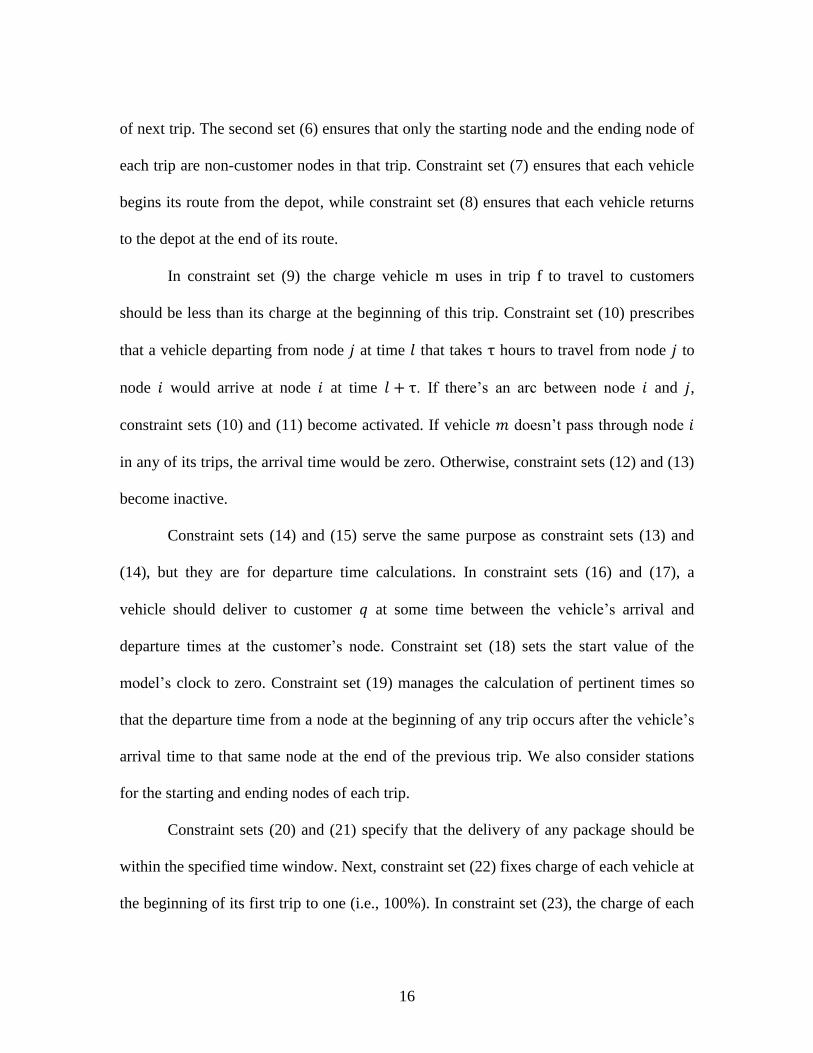
16

of next trip. The second set (6) ensures that only the starting node and the ending node of

each trip are non-customer nodes in that trip. Constraint set (7) ensures that each vehicle

begins its route from the depot, while constraint set (8) ensures that each vehicle returns

to the depot at the end of its route.

In constraint set (9) the charge vehicle m uses in trip f to travel to customers

should be less than its charge at the beginning of this trip. Constraint set (10) prescribes

that a vehicle departing from node 𝑗 at time 𝑙 that takes τ hours to travel from node 𝑗 to

node 𝑖 would arrive at node 𝑖 at time 𝑙 + τ. If there’s an arc between node 𝑖 and 𝑗,

constraint sets (10) and (11) become activated. If vehicle 𝑚 doesn’t pass through node 𝑖

in any of its trips, the arrival time would be zero. Otherwise, constraint sets (12) and (13)

become inactive.

Constraint sets (14) and (15) serve the same purpose as constraint sets (13) and

(14), but they are for departure time calculations. In constraint sets (16) and (17), a

vehicle should deliver to customer 𝑞 at some time between the vehicle’s arrival and

departure times at the customer’s node. Constraint set (18) sets the start value of the

model’s clock to zero. Constraint set (19) manages the calculation of pertinent times so

that the departure time from a node at the beginning of any trip occurs after the vehicle’s

arrival time to that same node at the end of the previous trip. We also consider stations

for the starting and ending nodes of each trip.

Constraint sets (20) and (21) specify that the delivery of any package should be

within the specified time window. Next, constraint set (22) fixes charge of each vehicle at

the beginning of its first trip to one (i.e., 100%). In constraint set (23), the charge of each

17

vehicle is restricted to be between zero and one. Constraint set (24) ensures that at the

end of each trip, if the vehicle enters a charging station, it is charged proportionally

according to the time spent at the station. However, no charging occurs at the depot.

Constraint sets (25) and (26) are resource limitation constraints. Constraint sets

(27) and (28) calculate the values of two variables. In set (27), if a particular vehicle

doesn’t go to any nodes, its arrival time to the depot at the final trip would be zero -- this

constraint becomes inactive. However, if it travels to any node, the vehicle’s arrival time

at the depot would be greater than zero and this constraint becomes active and the value

for the variable would be equal to one. It follows that this is used to compute the total

number of vehicles used. The same holds for set (28). If a charging station is used the

value of the second variable becomes equal to one, so sum of this variable for all of the

charging stations is equal to the number of stations used in the solution.

18

5. MODEL VALIDATION

A sample problem instance is defined to validate the model. Consider a fleet of

vehicles and a demand to deliver two packages each belonging to a unique customer.

Each vehicle may travel a maximum of 30 miles using a fully charged battery. The

distance between customers is given in Figure 1. By construction, it is not possible for

any vehicle to deliver both packages without recharging. Three charging stations are

available. It’s possible for any vehicle to leave the charging station with partially charged

battery. Full charge of an empty battery takes 8 hours, while partial charging time is

proportional to the charge gained during the recharge process. According to Table 1,

Customer 1’s package has to be delivered at 7 AM (exact time) and the package

belonging to Customer 2 has to be delivered within the time window from 10 AM to 10

PM.

19

Figure 1: Data for Test Instance

Table 1: Input Data for Example Problem

Time window (Customer 1) 7 AM – 7:01 AM

Time window (Customer 2) 10 AM – 10 PM

Vehicle range 30 miles

Recharge time 8 hours

After implementing the model in AMPL, the two-customer instance is evaluated

to minimize total number of vehicles required. The solution was produced using Gurobi

v.5.6 solver on a Windows 7 Enterprise platform with an Intel® Core™ i7-2600 CPU

processor @3.40 GHz. Optimal vehicle routes, remaining charge percentage, arrival and

0 1 3

4

5

2

A

A

A

Depot

Station

20 miles

30 miles

10 miles

A= node number

10 miles

Customer

20

departure times are shown in Figure 2. The optimal objective function value is 1.03 as

only one vehicle is used throughout the delivery process. The reason that the objective

value is 1.03 instead of 1 is that we have defined a small objective function term which

rewards the shortest return time to the depot (i.e., it eliminates long-journey solutions).

The vehicle first travels to customer one’s location because the package must be

delivered at 7 AM, before package two.

Because of its distance limitation associated with its range, the vehicle uses a

charging station after delivering the first package. The vehicle does a full charge due to

the distance to the next charging station within its route being equal to the maximum

vehicle range of 30 miles. The vehicle travels to customer two and uses a second

charging station in this trip, again because of the maximum distance limitation. Then, the

vehicle returns to the depot and again needs to use the third charging station due to its

maximum distance limitation. Therefore, the model proposes a travel schedule in which

the number of vehicles used is the minimum (one) and the number of charging stations

needed is three.

21

Figure 2: Results for Test Instance (objective is to minimize number of vehicles)

Now we run the model with a second objective: to minimize the number of

charging stations. Now, the objective function is equal to 2.03 (i.e., the model uses two

vehicles during the delivery process). Each vehicle delivers one package and each uses

one charging station in their route due to the maximum distance limit (Figure 3). The

vehicle delivering package one does not need a full charge when returning to the depot

0 1 3

4

5

2

- Key -

A=arrival time

B=departure time

C=remaining charge after

departing current node

100%

0.8 – 6.13

100%

7.8 – 15.8

16.6 – 16.6

100%

17 – 25

6.53 – 7

C%

A – B

Objective function (Z)

=1.0262

22

because its distance traveled is 10 miles less than the maximum distance limit. However,

the vehicle delivering package two requires a full charge while returning to the depot.

Therefore, two vehicles and minimum number of charging stations (two) are used to

deliver the packages. A comparison of the two models’ results is presented in Table 2. It

is clear that the different objective functions lead to completely different routes and

schedules.

Figure 3: Results for Test Instance (objective is to minimize number of stations)

0 1 3

4

5

2

- Key -

A=arrival time

B=departure time

C=remaining charge after

departing current node

100%

0.8 – 6.13

100%

10.4 – 15.73

9.6 – 10

100%

1.2 – 9.2

6.53 – 7

C%

A – B

66%

7.4 – 10.06

Vehicle 1

Vehicle 2

Objective function (Z)

=2.0278

23

Table 2: Comparison between Results

Objective

Min number of vehicles Min number of stations

Number of vehicles used 1 2

Number of stations used 3 2

24

6. MODEL PARAMETER ESTIMATION

In the proposed MIP model we use a number of 𝑀 (“big M”) parameters in the

constraint right hand sides. The use of 𝑀 as a constraint coefficient could result in

rounding errors that may cause the basis matrix (𝐵) to become singular. Also, there could

exist precision errors when computing 𝐵−1. Since 𝑀 is sometimes used to make

constraints active or inactive, even without basis matrix errors, large values of M could

cause commercial branch-and-bound solvers to work inefficiently or slower than desired.

Loose bounds can make it harder to prune nodes based on the objective function. In this

case, more nodes will be explored and the solving process can slow down. With this in

mind, we try to find smallest value for 𝑀 that works for the model.

In the optimization model, parameter 𝑒1 is used in objective function (1) and (2).

Parameter 𝑒1 is a coefficient multiplied by the summation of arrival times of all vehicles

to the depot. This parameter is important to ensure that each vehicle returns to the depot

as soon as possible and in order to eliminate unwanted idle time. We must make sure that

this coefficient does not impact the count of vehicles or charging stations used in the

model. In turn, we must ensure the value of second term in each objective function

should be less than one.

In the worst case, consider customer 𝑗 who has the maximum value of (any

customer time window upper bound value) + (travel time from customer to the depot). In

this case, 𝑒1 ∗ (∑ 𝑎0,𝑗,𝑡𝑉 ) would be maximal. This leads to the following estimation for

parameter 𝑒1:

25

𝑒1 < 1

𝑣 ∗ 𝑀𝑎𝑥𝑖∈𝐶 (𝛽𝑖 + 𝜏𝑖,0) .

(29)

Parameter 𝑀1 is used in constraint sets (10) and (11). This parameter is important

to make these constraints active or inactive as necessary. We need to estimate 𝑀1 only if

𝑥𝑗𝑖 is zero (if not, the parameter would have a zero multiplier and would be eliminated).

In the worst case, we estimate the value for parameter 𝑀1 as follows:

𝑀𝑎𝑥𝑖∈𝐶 (𝛽𝑖 + 𝜏𝑖,0) ≤ 𝑀1 . (30)

Parameter 𝑀2 is used in constraint sets (12) and (14). This parameter is important

in order to allow these constraints to become inactive as necessary. We must estimate a

value for this parameter only if ∑ 𝑥𝑗𝑖𝑛𝑜𝑑𝑒𝑠 is not equal to zero, so it could be any positive

integer (if not, parameter would have zero multiplier and would be eliminated). In worst

case, this term would be one; therefore, our estimate for 𝑀2 would be as follows:

𝑀2 ≥ 𝑎𝑖𝑚𝑓 . (31)

Further, as arrival time (𝑎𝑖𝑚𝑓) is estimated in the same way as for our 𝑀1 estimation, we

conclude that 𝑀2 is equal to 𝑀1.

Parameter 𝑀3 is used in constraint sets (25) and (26) in order to make these

constraints active or inactive. If 𝑒𝑚𝑓𝑛𝑔 is equal to one, in the worst case, parameter 𝑀3

would be greater than 𝑎𝑖𝑚𝑓. If 𝑒𝑚𝑓𝑛𝑔 is equal to zero then parameter 𝑀3 would be greater

than 𝑙𝑖𝑛𝑔. Arrival time (and similarly, departure time) is estimated in the same way we

26

did for our parameter 𝑀1 estimation. In general, 𝑀3 may be less than 𝑀1 but for

simplicity, we conclude that 𝑀3 is equal to 𝑀1.

Parameter 𝑒2 is used in constraint set (25). This constraint does not allow

simultaneous charging for distinct vehicles at the same station. In addition, we need this

parameter to avoid the possibility of similar arrival times (without this parameter if two

vehicles arrive at the same time, this constraint set does not work). In fact we block 𝑒2

time units before and after each arrival. A worst-case estimate for this parameter is as

follows:

𝑒2 <min(𝜏𝑖,𝑗)

𝑚𝑎𝑥 (𝛿𝑚)𝑣𝑒ℎ𝑖𝑐𝑙𝑒 𝑠𝑝𝑒𝑒𝑑

∗ μ . (32)

Parameter 𝑒3 is used in constraint sets (27) and (28). We need to estimate this

parameter only if 𝑎0𝑚𝑡 is not equal to zero (otherwise, the parameter would have a zero

multiplier and would be eliminated). In the worst case, our estimate for this parameter is

as follows:

𝑒3 < 1

𝑀𝑎𝑥𝑖∈𝐶 (𝛽𝑖 + 𝜏𝑖,0) .

(33)

27

7. EXPERIMENTAL STUDY

7.1. Experimental Plan

We analyze a set of 180 test instances, each with one depot, five customers, and

one charging station to evaluate the proposed model’s performance. All instances are

created based on the benchmark instances of Solomon (1987). The location of the depot

and customers is fixed in each instance, but various factor levels are considered: two

levels for vehicle range, three levels for recharge time, two levels for charging station

location, and two levels for time windows (Table 3). Instance set 𝑅1 has a short

scheduling horizon (time windows 𝑡1 − 𝑡8) while instance set 𝑅2 has a long scheduling

horizon (time windows 𝑡9 − 𝑡15). Figure 4 depicts a representation of depot, customers,

and candidate charging station locations.

Table 3: Experimental Design Parameters

Parameter Levels

Station Locations (61.7, 72.4)

(42.1, 64.9)

Time Windows See Table 4

Vehicle Range (𝛿) 100

150

Recharge Time (μ) 8

2.5

1

28

Figure 4: Instance Representation

L1 L2

0

10

20

30

40

50

60

70

80

0 20 40 60 80

Depot

Customers

Charging Station (level 1)

Charging Station (level 2)

29

Table 4: Experimental Time Window Data

Customer1 Customer2 Customer3 Customer4 Customer5

t1 start 161 50 116 149 34

end 171 60 126 159 44

t2 start 0 0 0 149 0

end 204 202 197 159 199

t3 start 151 40 106 139 24

end 181 70 136 169 54

t4 start 0 0 0 139 0

end 204 202 197 169 199

t5 start 133 22 98 123 20

end 198 87 143 184 93

t6 start 130 20 106 71 20

end 201 89 135 195 107

t7 start 15 18 54 138 20

end 204 202 187 169 199

t8 start 73 18 76 73 20

end 204 147 165 195 167

t9 start 707 143 527 678 34

end 848 282 584 801 209

t10 start 0 0 0 149 0

end 974 972 967 801 969

t11 start 658 93 436 620 20

end 898 333 676 860 260

t12 start 0 0 0 620 0

end 974 972 967 860 969

t13 start 636 74 498 470 20

end 919 351 613 965 370

t14 start 190 18 289 679 20

end 974 792 822 800 906

t15 start 451 18 378 477 20

end 974 534 733 965 610

30

7.2. Experimental Results and Analysis

Solutions are found by implementing the optimization model in AMPL and

solving it with Gurobi after imposing an optimization time limit, in order to minimize

number of vehicles used in the solution. The solution is produced using Gurobi solver on

a Windows 7 Enterprise platform with Intel® Core™ i7-2600 CPU @3.40 GHz. After

running our test instances, we see that in most cases, the objective function reaches a

stable value after 5-10 minutes of optimization time that does not change for several

hours. With this in mind, the optimization time limit for each run is set to 15 minutes. A

summary of the experimental results is shown in Tables 5 and 6 for the two time window

levels considered (𝑅1 and 𝑅2). The relative optimality gap is shown in Tables 7 and 8 for

the two time window levels considered (𝑅1 and 𝑅2).

For all instances, the near-optimal solution is to use either one or two vehicles to

deliver packages. Table 9 shows the percentage of test instances in which the resulting

near-optimal objective function recommends using one vehicle. This confirms that we

would need fewer vehicles if either vehicle range is increased, recharge time is decreased,

or scheduling horizon is increased.

31

Table 5: Experimental Results for Time Windows Set R1

μ=8 𝛿=100

μ=8 𝛿=150

μ=2.5 𝛿=100

μ=2.5 𝛿=150

μ=1 𝛿=100

μ=1 𝛿=150

Charging

Station

Location =

L1

t1 2.000059 2.000058 2.000059 2.000059 2.00006 2.000058

t2 2.00004 1.00003 2.000036 1.00003 2.000041 1.000029

t3 2.000044 2.000032 2.000044 2.000039 2.000044 1.000031

t4 2.000038 1.000028 2.000038 1.000027 2.000028 1.000026

t5 2.000037 2.000036 2.000041 2.000033 2.000039 1.000029

t6 2.000024 1.000054 2.000023 1.000024 2.000023 1.000024

t7 2.000029 1.000028 2.000039 1.000027 2.000029 1.000027

t8 2.000022 1.000023 2.000023 1.000022 2.000023 1.000023

Charging

Station

Location =

L2

t1 2.00006 2.000056 2.000059 2.000059 2.000059 2.000058

t2 2.00004 1.000029 2.00004 1.000029 2.000036 1.00003

t3 2.000044 2.00004 2.000045 2.000036 2.000044 2.000039

t4 2.000033 1.000027 2.000037 1.000027 1.000035 1.000027

t5 2.000042 2.000033 2.000042 2.000035 2.000042 1.00003

t6 2.000023 1.000025 2.000033 1.000025 2.000028 1.000024

t7 2.000029 1.000028 2.000029 2.000036 2.000039 1.000025

t8 2.000023 1.000022 2.000029 1.000022 2.000027 1.000015

Table 6: Experimental Results for Time Windows Set R2

μ=8 𝛿=100

μ=8 𝛿=150

μ=2.5 𝛿=100

μ=2.5 𝛿=150

μ=1 𝛿=100

μ=1 𝛿=150

Charging

Station

Location =

L1

t9 2.000148 1.000122 2.000135 1.000121 2.000132 1.000121

t10 1.000085 1.000026 1.00005 1.00003 1.000043 1.00003

t11 2.000114 1.000112 2.00012 1.00011 2.000114 1.000112

t12 1.00011 1.000108 1.000111 1.000107 1.00011 1.000108

t13 2.000108 1.000109 2.000111 1.000109 2.000114 1.000109

t14 1.00012 1.000117 1.00012 1.000118 1.00012 1.000117

t15 2.000093 1.000087 2.000093 1.000086 2.00009 1.000087

Charging

Station

Location =

L2

t9 2.000132 1.00012 1.000121 1.000122 1.000121 1.000121

t10 1.000076 1.000029 1.000044 1.00003 1.000035 1.000028

t11 1.000112 1.000112 1.000112 1.000113 1.000111 1.000112

t12 1.000108 1.000108 1.000107 1.000108 1.000108 1.000108

t13 1.000109 1.000108 1.000109 1.000108 1.000108 1.000109

t14 1.000118 1.000117 1.000118 1.000118 1.000118 1.000118

t15 1.000088 1.000087 1.000086 1.000086 1.000087 1.000085

32

Table 7: Relative Optimality Gap for Time Windows Set R1

μ=8 𝛿=100

μ=8 𝛿=150

μ=2.5 𝛿=100

μ=2.5 𝛿=150

μ=1 𝛿=100

μ=1 𝛿=150

Charging

Station

Location =

L1

t1 0.500970 0.002791 0.002791 0.500783 0.500970 0.002791

t2 0.501004 0.002973 0.501000 0.002973 0.501004 0.002973

t3 0.000048 0.501018 0.000086 0.501017 0.000096 0.000174

t4 0.500963 0.002808 0.500962 0.002808 0.500961 0.002808

t5 0.000100 0.001513 0.000090 0.001584 0.000077 0.500939

t6 0.500818 0.002463 0.000874 0.002463 0.001185 0.002791

t7 0.500970 0.002791 0.500970 0.002791 0.500970 0.002791

t8 0.500783 0.002383 0.500783 0.002383 0.500783 0.002372

Charging

Station

Location =

L2

t1 0.500963 0.001945 0.002808 0.001945 0.002808 0.001977

t2 0.501002 0.002969 0.501004 0.002973 0.501002 0.002960

t3 0.000069 0.000732 0.000075 0.000322 0.000097 0.000647

t4 0.500963 0.002808 0.500963 0.002806 0.500962 0.002808

t5 0.002305 0.001977 0.001191 0.471952 0.001945 0.001963

t6 0.500820 0.000322 0.500822 0.002464 0.001870 0.002452

t7 0.500970 0.002790 0.500970 0.002791 0.500970 0.002789

t8 0.500783 0.002383 0.500783 0.002370 0.500783 0.002790

Table 8: Relative Optimality Gap for Time Windows Set R2

μ=8 𝛿=100

μ=8 𝛿=150

μ=2.5 𝛿=100

μ=2.5 𝛿=150

μ=1 𝛿=100

μ=1 𝛿=150

Charging

Station

Location =

L1

t9 0.000985 0.012099 0.503452 0.010787 0.007017 0.010985

t10 0.501004 0.002972 0.005359 0.002973 0.004245 0.002973

t11 0.503044 0.011155 0.503045 0.011156 0.503045 0.011156

t12 0.010975 0.010717 0.010975 0.010713 0.010975 0.010716

t13 0.502915 0.010787 0.005968 0.010787 0.006066 0.010787

t14 0.503114 0.011678 0.011925 0.011679 0.011937 0.011674

t15 0.502455 0.008585 0.502333 0.008585 0.502334 0.008583

Charging

Station

Location =

L2

t9 0.402777 0.012100 0.010786 0.012098 0.011679 0.010717

t10 0.007534 0.002974 0.004484 0.002972 0.003663 0.011679

t11 0.011295 0.011152 0.011145 0.011149 0.011155 0.011155

t12 0.010716 0.010717 0.010716 0.010716 0.010717 0.011295

t13 0.010985 0.010786 0.010786 0.010786 0.010784 0.011679

t14 0.011679 0.011679 0.011679 0.011678 0.011677 0.010975

t15 0.008731 0.008586 0.008586 0.008586 0.008586 0.005968

33

Table 9: Percentage of Instances Able to Use Only One Electric Vehicle

Time Window Set R1 Time Window Set R2

𝜹=100 𝜹=150 𝜹=100 𝜹=150

μ=8 0 % 62 % 64 % 100 %

μ=2.5 0 % 56 % 71 % 100 %

μ=1 6% 81 % 71 % 100 %

34

CONCLUSIONS AND FUTURE WORK

A mixed-integer programing (MIP) formulation is developed to solve the partially

rechargeable electric vehicle routing problem with time windows and capacitated

charging stations. The analysis of this model gives insights about the optimal design

combination of charging stations and electric vehicle fleet sizing needed for parcel

delivery. This analysis confirms that fewer vehicles are needed if systems designers are

able to increase vehicle range, decrease recharge time, or increase their scheduling

horizon.

Due to the problem's NP-hard complexity (via reduction to the classical VRP),

our solution is not optimal. In fact, for larger test instances with more than five

customers, we may not reach even a good solution in an appropriate amount of time. In

future work, this research can be extended to develop heuristic or metaheuristic

algorithms to achieve better results for larger instances in a timely fashion.

35

REFERENCES

[1] G. B. Dantzig and J. H. Ramser (1959) The truck dispatching problem. Management

Science, 6:80-91

[2] B. Crevier, J.-F. Cordeau, and G. Laporte. (2007) The multi-depot vehicle routing

problem with inter-depot routes. European Journal of Operational Research,

176(2):756-773

[3] F. Goncalves, S. R. Cardoso, Relvas S., and A. P. F. D Barbosa-P_ovoa. Optimization

of a distribution network using electric vehicles: A VRP problem. Technical report, CEG-IST, UTL, Lisboa, 2011.

[4] S. Erdogan and E. Miller-Hooks. A green vehicle routing problem. Transportation

Research Part E: Logistics and Transportation Review, 48(1):100-114, 2012.

[5] Bard, J., Huang, L., Dror, M., Jaillet, P., 1998. A branch and cut algorithm for the VRP

with satellite facilities. IIE Transactions 30, 821–834.

[6] M. M. Solomon. Algorithms for the vehicle routing and scheduling problems with time

window constraints. Operations Research, 35(2):254-265, 1987.

[7] Schneider M, Stenger A, Goeke D (2014) The electric vehicle-routing problem with time

windows and recharging stations. Transportation Science [8] Tarantilis CD, Zachariadis EE, Kiranoudis CT (2008) A hybrid-guided local search for

the vehicle routing problem with intermediate replenishment facilities. INFORMS J.

Comput.20(1):154–168.

[9] Bektas T, Laporte G (2011) The pollution-routing problem. Transportation Res. Part B

45(8):1232-1250

[10] Mehrez A, Stern HI (1985) Optimal refueling strategies for a mixed vehicle fleet. Naval

Res. Logist. Quart. 32(2):315–328.

[11] Ichimori T, Ishii H, Nishida T (1983) Two routing problems with the limitation of fuel.

Discrete Appl. Math. 6(1):85–89.

[12] Jabali O, Van Woensel T, de Kok AG (2012) Analysis of travel times and CO2

emissions in time dependent vehicle routing. Production Oper. Management 21(6):1060–1074

[13] Conrad RG, Figliozzi MA (2011) The recharging vehicle routing problem. Proc. 2011

Indust. Engrg. Res. Conf., Reno, CA. [14] Taha M, Fors N, Shoukry A (2014) An Exact solution for a class of green vehicle routing

problem. Ind Eng and Operations Management. Conf., Bali, Indonesia. [15] Hiermann G, Puchinger J, Hartl R (2014) The electric fleet size and mix vehicle routing

problem with time windows and recharging stations. Submitted to Transportation Science

[16] Yang J, Sun H (2014) Battery swap station location-routing problem with capacitated

electric vehicles. Computers & operations research (accepted manuscript)

[17] Albrecht A, Pudney P (2013) Pickup and delivery with a solar-recharged vehicle.

National conference of the Australian society for operations research [18] Cassandras C, Wang T, Pourazarm S (2014a) Energy-aware vehicle routing in networks

with charging nodes. Working paper

[19] Cassandras C, Wang T, Pourazarm S (2014b) Optimal routing of energy-aware vehicles

in networks with inhomogeneous charging nodes. Working paper

36

[20] Worley O, Klabjan D, Sweda T (2014) Simultaneous vehicle routing and charging

station siting for commercial electric vehicles. Working paper

[21] Schneider M, Stenger A, Hof J (2014) An Adaptive VNS algorithm for Vehicle Routing

Problems with Intermediate Stops. Technical report [22] Preis H, Frank S, Nachtigall K (2013) Energy-optimized routing of electric vehicles in

urban delivery systems. Operations Research Proceedings, pp 583-588

[23] Preis H, Frank S, Nachtigall K (2014) On the modeling of recharging stops in context of

vehicle routing problems. Operations Research Proceedings, pp 129-135