The Painleve paradox in contact mechanics

Alan R. Champneys, Peter L. Varkonyi

final version 11th Jan 2015

Abstract

The 120-year old so-called Painleve paradox involves the loss of determinism in models ofplanar rigid bodies in point contact with a rigid surface, subject to Coulomb-like dry friction.The phenomenon occurs due to coupling between normal and rotational degrees-of-freedomsuch that the effective normal force becomes attractive rather than repulsive. Despite a richliterature, the forward evolution problem remains unsolved other than in certain restrictedcases in 2D with single contact points. Various practical consequences of the theory arerevisited, including models for robotic manipulators, and the strange behaviour of chalkwhen pushed rather than dragged across a blackboard.

Reviewing recent theory, a general formulation is proposed, including a Poisson or en-ergetic impact law. The general problem in 2D with a single point of contact is discussedand cases or inconsistency or indeterminacy enumerated. Strategies to resolve the paradoxvia contact regularisation are discussed from a dynamical systems point of view. By passingto the infinite stiffness limit and allowing impact without collision, inconsistent and inde-terminate cases are shown to be resolvable for all open sets of conditions. However, twounavoidable ambiguities that can be reached in finite time are discussed in detail, so calleddynamic jam and reverse chatter. A partial review is given of 2D cases with two points ofcontact showing how a greater complexity of inconsistency and indeterminacy can arise. Ex-tension to fully three-dimensional analysis is briefly considered and shown to lead to furtherpossible singularities. In conclusion, the ubiquity of the Painleve paradox is highlighted andopen problems are discussed.

KEYWORDS: rigid body ; Painleve paradox ; Coulomb friction ; impact mechan-ics; dynamic jam ; sprag-slip oscillation ; chatter ; Zeno phenomenon ; reverse chat-ter ; impact without collision ; inconsistency ; indeterminacy ; rational mechanics.

1 Introduction

Paul Painleve is a truly remarkable figure in the history of science and technology. In mathe-matics, Painleve is most closely associated with the family of integrable differential equations andcorresponding transcendental functions that bear his name. But there is much more to Painleve,[8]; he made pivotal contributions to the theory of gravitation, he was possibly the first ever air-craft passenger (taking a seat in the Wright brother’s plane in 1908) and set up the world’s firstdegree in programme in Aerospace Engineering. His role as Minister of Public Instruction andInventions, led to him being appointed Prime Minister of France briefly during the First WorldWar, and again in 1924. In the latter stint he was forced to resign after being unable to solve

1

arX

iv:1

601.

0354

5v1

[ph

ysic

s.cl

ass-

ph]

14

Jan

2016

the overriding financial crisis of the time (an uncanny parallel to 21st Century European politics,perhaps).

This paper shall look at the legacy of Painleve’s work in rigid body mechanics, specificallythe rather curious phenomena that are present in models of dry friction. In a series of papersstarting in 1895 [61, 62, 63], Painleve provided simple examples which illustrate a fundamentalinconsistency in the laws of Coulomb friction. (Technically, we should refer to Amontons-Coulombfriction, because the laws were first postulated by Amontons at the beginning of the 18th Century,whereas Coulomb’s role was one of experimental verification, see e.g. [33, 19]. As with many unjustattributions in science, Amontons’ name seems to have been dropped from the epithet now usedto describe the simplest law of dry friction. In fact, theory that additionally involves solving forthe normal force at contact is sometimes called the Signorini-Coulomb model or the Signorini-Amontons-Coulomb . . ., but we shall just refer to Coulomb friction in what follows.) The so-calledPainleve paradox (which, to add more historical accuracy, as Painleve acknowledges, was firstdiscovered by Jellet [35]) occurs in planar bodies undergoing oblique contact for which there is asufficiently large coupling between normal and tangential degrees of freedom at the contact point.Such configurations, given sufficiently high coefficient of friction, can reach a point where thereis no longer a unique forward simulation — either a multiplicity of possibilities (indeterminacy),or none (inconsistency) — so there is no way to decide what happens next within rigid bodymechanics. Further historical remarks on the origins of the Painleve paradox can be found in thebooks by Brogliato [10] and and Le Suan Anh [4].

The configuration most closely associated with Painleve is that of rod falling under gravitywhose lowest end is in contact with a horizontal surface and subject to simple Coulomb friction,see Fig. 2. We shall refer to this as the classical Painleve problem (CPP), although, as pointedout by Leine [43], this was not actually the example that Painleve considered first (see Sec. 2).

The CPP can be realised using a pencil that is momentarily balanced on its tip on a roughpiece of paper attached to a rigid horizontal table. Upon letting go, minor disturbances mean thepencil will have a shallow angle to the vertical and will start to fall. Initially, the tip remains fixed,forming a pivot about which the pencil rotates. Upon reaching some critical angle, the tangentialforce at the tip will be large enough for the pencil to begin to slip (in the opposite direction tothe instantaneous horizontal velocity component of the top). A faint line begins to appear on thepaper. As the pencil continues to fall, before it becomes fully horizontal, the angular accelerationwill be sufficient to overcome the vertical component of the ground reaction force at the tip. Thus,the tip lifts off and the faint line is terminated. A fraction of a second later, the blunt end of thepencil hits the table, some rattling motion ensues, before the pencil becomes fully horizontal, rollsfor a while and comes to rest on the table. No paradox.

What Painleve realised though is that if the coefficient of friction is large enough (in fact,unrealistically large for an approximately uniform rod like a pencil on anything other than thecoarsest sandpaper) then something else can happen. Before the pencil lifts off, it can reach aconfiguration that is now known as dynamic jam where one cannot decide with certainty whathappens next. The pencil tip could lift off in the usual way with an initially infinitesimal normalvelocity. Or, the pencil could remain in contact such that the more it tries to lift off, the moreit rotates and digs back down into the surface. It is as if there is a negative normal force pullingthe tip into the surface. If one adds a rigid impact model, like Newton’s law of restitution, tothe mechanical formulation, then such a force causes a so-called impact without collision (IWC)[10, Ch. 5.5], see Sec. 3.2 below. Such an impact involves an impulsive jump to reduce the tip’sslipping velocity to zero and eject it from the surface with a finite normal velocity. We give amore quantitative description of the paradox for the CPP in Sec. 2.2 below.

2

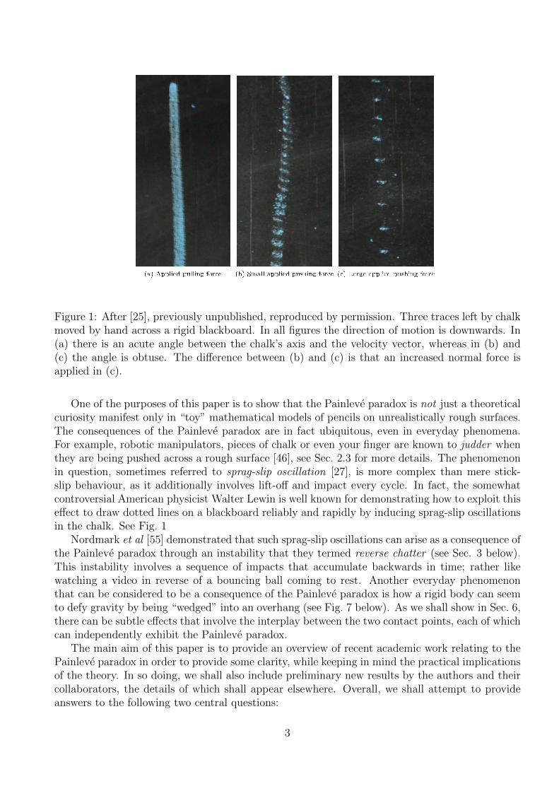
Figure 1: After [25], previously unpublished, reproduced by permission. Three traces left by chalkmoved by hand across a rigid blackboard. In all figures the direction of motion is downwards. In(a) there is an acute angle between the chalk’s axis and the velocity vector, whereas in (b) and(c) the angle is obtuse. The difference between (b) and (c) is that an increased normal force isapplied in (c).

One of the purposes of this paper is to show that the Painleve paradox is not just a theoreticalcuriosity manifest only in “toy” mathematical models of pencils on unrealistically rough surfaces.The consequences of the Painleve paradox are in fact ubiquitous, even in everyday phenomena.For example, robotic manipulators, pieces of chalk or even your finger are known to judder whenthey are being pushed across a rough surface [46], see Sec. 2.3 for more details. The phenomenonin question, sometimes referred to sprag-slip oscillation [27], is more complex than mere stick-slip behaviour, as it additionally involves lift-off and impact every cycle. In fact, the somewhatcontroversial American physicist Walter Lewin is well known for demonstrating how to exploit thiseffect to draw dotted lines on a blackboard reliably and rapidly by inducing sprag-slip oscillationsin the chalk. See Fig. 1

Nordmark et al [55] demonstrated that such sprag-slip oscillations can arise as a consequence ofthe Painleve paradox through an instability that they termed reverse chatter (see Sec. 3 below).This instability involves a sequence of impacts that accumulate backwards in time; rather likewatching a video in reverse of a bouncing ball coming to rest. Another everyday phenomenonthat can be considered to be a consequence of the Painleve paradox is how a rigid body can seemto defy gravity by being “wedged” into an overhang (see Fig. 7 below). As we shall show in Sec. 6,there can be subtle effects that involve the interplay between the two contact points, each of whichcan independently exhibit the Painleve paradox.

The main aim of this paper is to provide an overview of recent academic work relating to thePainleve paradox in order to provide some clarity, while keeping in mind the practical implicationsof the theory. In so doing, we shall also include preliminary new results by the authors and theircollaborators, the details of which shall appear elsewhere. Overall, we shall attempt to provideanswers to the following two central questions:

3

Question 1. For a given rigid body system with contact, in a given state at a given instanceof time, is there a uniquely defined forward-time continuation of the dynamics within theformalism of rigid body mechanics? This divides naturally into two subquestions: is anypossible forward continuation possible (consistency), and, if so, is it unique (determinacy)?

Question 2. Given a rigid body system that is not exhibiting the Painleve paradox at one in-stance of time, what possible ways can it enter into a Painleve paradox state at a laterin time? Again there are two subquestions: how unlikely is it to enter an inconsistent orindeterminate state; and what happens next?

As we shall show, no complete answer to either question is yet known. Nevertheless, we shallattempt to provide partial answers, restricted to the case of a single point contact in two spatialdimensions. As we shall see though, there are way more possibilities that need consideration in 3Dor in the presence of several isolated point contacts, for which we can only provide partial results.For more physically realistic problems with regional (line or patch) contacts, almost nothing isknown. Therefore in this paper we shall restrict attention to problems with a finite number ofisolated point contacts.

Another aim of this paper is steer a path through the various approaches that have been pro-posed to resolve the Painleve paradox from both a practical and a rational, analytic point of view.Our focus is not particularly on numerical methods for simulation in the presence of the paradox,although it is worth pointing out recent results for example in [1, 70, 71]. Nor do we considercontrol algorithms designed to avoid Painleve paradoxes in robotic systems, but see e.g. [10, 18]for recent results. Instead, we shall attempt to understand the dynamical consequences of thePainleve paradox from a mathematical modelling point of view, building on recent understandingof the theory of piecewise-smooth dynamical systems see [20, 42, 16, 15], In fact, it is well knownthat piecewise-smooth systems of Filippov-type [20] can exhibit nonuniqueness or nonexistence ofsolutions, see e.g. [20, 5, 34].

Philosophically speaking, the Painleve paradox is not a puzzle about the real world, but afailure of a theory based on rigid body mechanics and Coulomb friction to provide completeunequivocal descriptions of dynamics. In truth, any physical resolution of the Painleve paradoxtends to involve relaxing some of the assumptions of rigid body mechanics in order to predictwhat happens next, see Sec. 4. In effect, the Painleve paradox provides insight into points ofextreme sensitivity in rigid body mechanics where additional physics, possibly at the microscale,is required in order to accurately capture the dynamics. Such points of extreme sensitivity aretypically going to be observable as points where significant changes can result from minusculevariations of the physical properties or initial states of the bodies involved. A key question to beaddressed then is:

Question 3. Given a rigid body system with contact whose forward evolution is either incon-sistent or indeterminate, what is the minimal extra modelling ingredient in order for thereto be a unique forward evolution in all inconsistent and indeterminate cases? Which casescan be made uniformly resolvable via this approach; by which we mean, if the additionalingredient to the theory arises through a small parameter ε, does a qualitatively consistentoutcome occur uniformly in the limit as ε→ 0?

The rest of this paper is outlined as follows. Section 2 contains a historical introduction to thesubject. A mathematical explanation of the paradox is given in terms of the CPP. This is followedby a discussion of the role of different friction laws, a description of other simple configurationsthat feature the Painleve paradox and a brief review of the various attempts to resolve the paradox.

4

θX

Y

λ

λ N

T

g

l

l

c.o.m

P

Figure 2: The classical Painleve problem (CPP) for a falling rod.

Section 3 then introduces a general formulation for the simplified case of a planar system with asingle contact. An attempt is made to answer Question 1 by enumerating all the different casesthat lead to inconsistency or indeterminacy. We also discuss how to augment the formulation byincluding an impact law, and discuss the possibility of the accumulation of impacts via chatter(also known as the Zeno phenomenon). Section 4 then looks at Question 3 by adding complianceinto the model in order to find cases that are uniformly resolvable. Section 5 considers Question 2for the 2D single contact case; the theory of Genot and Brogliato [22] is reviewed and generalised,to show cases where dynamic jam must occur. We also consider whether the Painleve paradoxcan be approached through chatter and consider conditions under which reverse chatter can betriggered. Section 6 considers extensions to the theory for configurations with two or more contactpoints and starts to enumerate the additional paradoxes that can occur. Section 7 then brieflyconsiders the single-contact problem in 3D, illustrating that a different kind of dynamic jam canoccur which does not involve the singularity analysed in [22]. Finally, Section 8 draws conclusions,highlights open problems and and makes philosophical remarks.

2 Historical perspective

2.1 The classical Painleve problem

The CPP, first proposed by Painleve in 1905 [63], involves a slender rigid rod falling under gravitywhile in contact with a rigid, stationary, frictional horizontal surface. Suppose the rod has massm and radius of gyration r, that the centre of mass is a distance ` from the contact point P , andthat λN ≥ 0 and λT are the normal and tangential components of contact force. Let (X, Y ) bethe Cartesian co-ordinates of the rod’s centre of mass within the plane in which it is falling, andθ be its angle to the horizontal, as depicted in Fig. 2 (note that for convenience we have chosenan angle θ which is π minus the angle of the same name used in [22]). Then, under the usualassumptions of Lagrangian mechanics, the equations of motion can be written as

mX = −µλT , mY = −mg + λN mr2θ = −`(cos θλN + µ sin θλT ). (1)

Let(x, y) := (X + ` cos θ, Y − ` sin θ), and (u, v) := (x, y)

represent the generalised tangential and normal co-ordinates and velocities at P . Then, λN in (1)can be considered to be a dynamic Lagrange multiplier that is used to maintain the inequality

5

constraint y ≥ 0. In particular λN and y are said to satisfy a complementarity relation λN ⊥ y > 0,which means that at most one of λN and y can be positive (see e.g. [10]). Whenever y = 0, weassume a simple Coulomb friction law:

|λT | ≤ µ|λN |, λT = −µ sign(u)λN for u 6= 0, (2)

where µ is the coefficient of friction.Now, suppose there is an initial condition such that the rod is slipping with u > 0 and

0 < θ < π/2, so that λT = −µλN . Then, using (1), the normal acceleration can be written as

y = Y + `(θ2 sin θ − θ cos θ) ,

= (`θ2 sin θ − g) +

[1 +

`2

r2cos2 θ − µ cos θ sin θ)

]λNm

,

:= b(θ, θ) + p+(θ, µ)λN . (3)

Equation (3) describes the dynamics of the CPP in the normal direction at the contact point,in terms of two scalar quantities b which describes the free normal acceleration in the absence ofany contact forces and p+ which we shall refer to as the “degree of Painleve -ness” or the Painleveparameter. In fact, the rest of this paper shall make extensive use of these two dynamic scalarquantities (and a third, p−, the equivalent of p+ for slipping in the other direction) for quite generalclasses of contact problems. As we shall see in Sec. 2, b will always be a function of generalisedvelocities and co-ordinates, whereas for stationary contact surfaces p± are functions of positionvariables and properties of the friction law only.

In the case of the CPP, equation (3) shows that if the rod starts at rest in the near verticalposition (with an angle θ just smaller than π/2), then clearly b < 0 and p+ > 0 initially. Moreoverb and p+ are smooth functions of dynamic variables so, as long as the rod maintains the conditionu > 0 for slip, these quantities will evolve smoothly and preserve their signs for small times.Hence, for sufficiently short times there is a unique normal force

λN = −b/p+ > 0 (4)

that makes the normal acceleration in (3) vanish, so that the rod remains in contact while it falls.Similarly if θ is initially small and positive so that the rod is close to horizontal then b < 0

and p+ > 0. However, for intermediate angles, depending on other parameters and velocities, p+

and b may in general take either sign. So let us analyse what happens at a time when either p orb smoothly changes sign during motion.

A point where b passes from negative to positive (while p+ remains positive) is easy to analyse.This would represent a point at which the rod simply lifts off from the surface. The normal force(4) smoothly tends to zero, the dynamics would lift off into free motion with y(t) > 0 and λN = 0.

The case of negative p+ is much more unusual. First, consider the possibility of p+ < 0 andb < 0. Here, the free acceleration b pushes the tip of the rod down towards the surface. Howeverthe normal force given by (4) would be negative, which violates our complementarity assumption.A positive reaction force λN would cause acceleration in the same direction as b, pushing the roddown further into the surface, precluding any vertical equilibrium. The rod cannot remain incontact with the surface, ergo it must lift off. But it can’t because if we look for free motion withλN = 0, the free acceleration b < 0 takes us back into contact. Thus, we have a configuration thatis inconsistent, and there is no valid continuation of the motion forwards in time.

6

Consider instead an initial conditions for which p+ < 0 and b > 0. Here, in the absence of anycontact forces, the rod would simply lift off with λN = 0. However there is another possibility;there is now a unique non-zero normal force λN = −b/p > 0 for which the free normal accelerationb is equilibrated. So the rod could remain in contact. Hence, this case is indeterminate, becausethere is non-uniqueness in possible outcome.

It is useful to consider the conditions under which these paradoxes could occur in the CPP.The condition p < 0 can be written

µ > µP (θ) :=r2 + `2 cos2 θ

`2 sin θ cos θ. (5)

Now, in the case of a uniform rod for which r2 = 13`2, we see that µp is minimised when θ = arctan 2,

in which case we can find the minimum coefficient of friction for which there exists a value for θfor which p+ < 0, namely µP,min = 4/3. Thus, for µ > µP,min an interval of angles θ exists suchthat p+ can be negative.

So what does happen for the falling rod if µ > µP,min? This question was analysed in detailby Genot and Brogliato [22] (see also [93] for a modern re-interpretation). They show that thereis a µc = 8/(3

√3) > 4/3 = µP,min, for the case of the uniform rod, such that for µ < µc there can

be no initial condition that approaches p+ = 0 during slipping, the rod must lift off first. But forµ > µc then there is a thin wedge of initial conditions (θ, θ) for which a paradox can be reached.However they show that there can be no entry during forward slipping into regions with p+ < 0,the only way to get there is via reaching a configuration where simultaneously b = p+ = 0, whichis precisely what Or & Rimon [60] define as dynamic jam. As we shall see in Sec. 5, the method ofGenot and Brogliato, involves rescaling time so that the point b = p = 0 becomes an equilibriumpoint in a pseudo phase plain, which can attract an open set of initial conditions. In deference toGenot, we shall call this special point the G-spot. What happens after the G-spot is reached isnot clear.

2.2 Is the paradox due to unrealistic friction models?

One simple possible resolution of the Painleve paradox is that a coefficient of friction µ = 4/3 isunrealistically large, with typical values for most materials being significantly less than 1 (althoughvalues as large as 2 have been proposed for rubber-on-rubber contacts). This resolution is speciousthough because it is easy to formulate mechanisms for which µP,min is significantly smaller. Forexample, if we allow the rod in the CPP to be non-uniform, then µP,min is a function of the radiusof gyration r. Taking the limit that all the mass is concentrated at the centre of mass, then r → 0and the formula (5) shows that µP,min becomes vanishingly small in this limit.

Another possible resolution is that the Coulomb friction law is too simplistic and that if a“more realistic” friction model is used, the Painleve effect will disappear. This may be possiblefor certain cases and configurations, but seems unlikely in general. For example, Liu et al [46]find the paradox to still be present in a model that has a different dynamic and static coefficientof friction. In addition, there is a trivial indeterminacy if, as is typical for such models, the staticcoefficient of friction is higher than the dynamic one.

Grigoryan [24] proposes that the CPP can be resolved by replacing the Coulomb friction lawwith a smoothed version in which λT is a smooth function of u with large finite slope at u = 0.Philosophically, this is equivalent to replacing dry friction with viscous friction for low velocities.However, he studies only a single rather artificial model, the so-called Painleve -Klein problem(see Sec. 2.3) and the resolution doesn’t seem to satisfy our definition of uniform resolvability

7

θ

Y

X

λ

λ

T

N

g

Figure 3: The original problem posed by Painleve of a slipping block

in the limit that the slope tends to infinity. Also, Ivanov [32] claims that such friction lawsintroduce further non-uniqueness in place of non-existence. If instead we replace Coulomb lawwith a Stribeck law (see e.g. [41]) in which there is still a jump at u = 0 but µ is taken to bea smooth function of u, then the above calculations for the CPP can be easily repeated. It isstraightforward to show that in principle, there is no impediment to p± becoming negative in thiscase too. The same conclusion holds if µ is a function of position x or some internal state variablesuch as in rate-and-state friction models (see [68] and references therein).

There is a rich literature on detailed microscopic friction modelling, indeed tribology is a fieldin its own right, which we shall not explore further here. Even simple models of tangential friction,ignoring the dynamics in normal directions, can give rise to complex dynamics such as stick-slipvibrations and “squeal”; see for example the reviews [91, 38, 19]. Clearly, when dealing withthe Painleve paradox, the details of what happens in practice are going to depend sensitively onthe precise friction characteristics. Nevertheless, it is our contention that the Painleve paradoxis fundamentally due to the nature of the coupling between normal and tangential degrees offreedom, rather than to specific properties of the friction law. Therefore, throughout the restof this paper, for simplicity, we assume the simple Coulomb law (2), with a single coefficient offriction µ.

2.3 Other mechanical configurations

In fact, as pointed out by Leine et al [43], the original problem studied by Painleve in 1895 [61]was not the CPP but that of a planar box slipping down a rough plane that is inclined at a shallowangle to the horizontal; see Fig. 3. The box is assumed to be in point contact at its lowest cornerand to be subject to Coulomb friction. As Leine et al show, the simplest model of this problemis actually dynamically equivalent to the CPP (although see [48] for a more general analysis) andthe minimum value of friction coefficient required is identical. In particular, just as with the CPP,if we allow the box to have inhomogeneous mass distribution, then µP,min can in theory be as smallas we like.

As mentioned in the introduction, the motion of chalk being pushed across a blackboard isoften proposed as a classroom illustration of the Painleve paradox. In particular, if the chalk isdragged (which would correspond to an angle θ in the second quadrant if motion is to the right inFig. 2), then a uniform straight line is generally seen. However, if the angle is in the first quadrantand a large force is applied, then the chalk can undergo a series of hops [25]. Such sprag-sliposcillations were reproduced by Hoffmann and Gaul [27] in various models with compliance at thetip. These oscillations are at least reminiscent of the Painleve property because lift-off appears to

8

m 2

(a)

1m

belt velocity

m

m

λ

λ

1

2

N

T

(b)

Figure 4: The frictional impact oscillator and its simplification, as studied in [43]

occur despite the chalk being pressed into the board. Such an explanation is not sufficient howeverbecause the coefficient of friction for chalk on a blackboard is likely to be significantly less thanµP,min = 4/3. However, the contact mechanics of chalk, a cylinder that is typically only in contactalong part of its end, is likely to be more complex than that of an ideal rod, and we also haveto take account of the body forces and controls being applied by the teacher. Moreover, we shallalso see in Sec. 5 that another explanation for the onset of the hopping motion, namely reversechatter, can be triggered upon the transition from stick to slip, even if p± remain positive. IndeedNordmark et al [55] show that an open-loop controller implementing a vander-Pol-like body forceto a simple rod model can trigger reverse chatter that saturates into limit-cycle motion.

A laboratory demonstration of sprag-slip oscillations can be made through a pin-on-disk rig, ifthe the pin is allowed to contact obliquely and to lift off [30]. Such experimental apparatus is oftenused to categorise friction-induced ‘brake squeal’ vibrations, see for example [12]. Inspired by suchsystems, Leine et al. [43] studied a so-called frictional impact oscillator, see Fig. 4. They showedthat under suitable choices of parameters the condition for the Painleve property to hold can bewritten as µP,min = 2

√m1/m2, which of course can take arbitrarily small values if the second mass

is much heavier than the first. They found that finite-amplitude stable periodic motion can occurin the Painleve parameter region that comprises phases of free motion, sticking and slipping. Theonset of this motion typically occurs via a subcritical Hopf bifurcation from the steady stickingsolution.

A related practical manifestation of sprag-slip oscillation is the hopping motion that is some-times observed in finger-like robotic manipulators [10]. Inspired by this, in a series of papersculminating in [94], Liu, Zhao, Chen and their co-workers have studied theoretically, numericallyand experimentally the motion of the two-link robotic manipulator depicted in Fig. 2.3(a). Inparticular, in [46] they found precise formula for µP,min, which tends to zero as the height H → 0.They were also able to simulate bouncing motion corresponding to a concatenation of stick, slip,free flight and impact. That such hopping motion is attributable to the Painleve paradox is nowwell established in the robotics literature, and work instead has begun to look at how to controlsuch unwanted behaviour (e.g. [18, 45]).

There are also possible applications of these ideas in bio-mimicry of sensing systems. Forexample, mammals such as rats, have slender tapered rod-like whiskers that repeatedly sweep andtap on a surface at oblique angles, see e.g. [67]. The motion of the tip of a rat’s whisker seems

9

belt velocity

λ

λ

N

T

θ

θ2

1

H

(a) (b)

Figure 5: (a) The two-link robotic manipulator [46]. (b) The inverted pendulum on slider [60].

λ N

λ T

λ N

λ T2

1

2

µ 2

µ

1

1

φ

Figure 6: The Painleve-Klein problem

akin to sprag-slip oscillation, but driven by a regular circular motion from the follicle. It wouldappear that the combined effects of stick-slip and lift-off from the tip, fed back along the whiskerenable the rat to sense both texture and compliance of the surface.

Another experimentally amenable Painleve paradox demonstrator was proposed by Or & Ri-mon [60], the so-called inverted pendulum on a slider, see Fig. 2.3(b). They were able to findexplicit expressions for initial conditions and parameters that would lead to dynamic jam in such adevice. They found the explicit expression µP,min =

√(2(1 +m1/m2)(1 + ρ2/r2)− 1)2 − 1, which

can be chosen to be experimentally accessible by choosing appropriate values for the configurationconstants m1, m2 r2 and ρ2.

A less explored, but potentially industrially important area in which the Painleve paradox canapply is in rotating machinery. Here there may be large coupling between normal and tangentialdegrees of freedom due to gyroscopic forces. For example Wilms & Cohen [90] report that thePainleve effect can be seen the motion of rotating shaft whose bearing is subject to coulombfriction. Kozlov [39] studies a brake shoe problem that exhibits the Painleve paradox, which heclaims was resolved by Neimark and co-workers [52] by introducing longitudinal and transverseelasticity, see Sec. 2.4.

All of the above examples correspond to cases with a single point contact. There is less in theliterature on the Painleve paradox occurring in problems with multiple contacts. The Russianliterature tends to use as the canonical model, not the CPP but the so-called Painleve-Kleinproblem, see [32, 52, 88, 24, 3]. A good summary discussion of work on this problem is given in

10

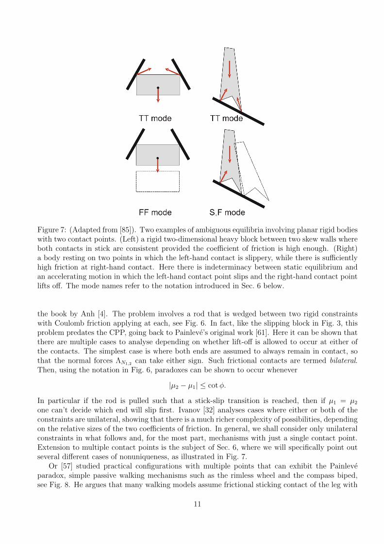
Figure 7: (Adapted from [85]). Two examples of ambiguous equilibria involving planar rigid bodieswith two contact points. (Left) a rigid two-dimensional heavy block between two skew walls whereboth contacts in stick are consistent provided the coefficient of friction is high enough. (Right)a body resting on two points in which the left-hand contact is slippery, while there is sufficientlyhigh friction at right-hand contact. Here there is indeterminacy between static equilibrium andan accelerating motion in which the left-hand contact point slips and the right-hand contact pointlifts off. The mode names refer to the notation introduced in Sec. 6 below.

the book by Anh [4]. The problem involves a rod that is wedged between two rigid constraintswith Coulomb friction applying at each, see Fig. 6. In fact, like the slipping block in Fig. 3, thisproblem predates the CPP, going back to Painleve’s original work [61]. Here it can be shown thatthere are multiple cases to analyse depending on whether lift-off is allowed to occur at either ofthe contacts. The simplest case is where both ends are assumed to always remain in contact, sothat the normal forces ΛN1,2 can take either sign. Such frictional contacts are termed bilateral.Then, using the notation in Fig. 6, paradoxes can be shown to occur whenever

|µ2 − µ1| ≤ cotφ.

In particular if the rod is pulled such that a stick-slip transition is reached, then if µ1 = µ2

one can’t decide which end will slip first. Ivanov [32] analyses cases where either or both of theconstraints are unilateral, showing that there is a much richer complexity of possibilities, dependingon the relative sizes of the two coefficients of friction. In general, we shall consider only unilateralconstraints in what follows and, for the most part, mechanisms with just a single contact point.Extension to multiple contact points is the subject of Sec. 6, where we will specifically point outseveral different cases of nonuniqueness, as illustrated in Fig. 7.

Or [57] studied practical configurations with multiple points that can exhibit the Painleveparadox, simple passive walking mechanisms such as the rimless wheel and the compass biped,see Fig. 8. He argues that many walking models assume frictional sticking contact of the leg with

11

(b)(a)

Figure 8: (a) The rimless wheel and (b) the compass biped configurations studied in [57, 21].

the ground. Allowing perturbations that involve foot slippage, he shows that regular gait periodicsolutions can be subject to an instability that is closely related to dynamic jam. Dynamicalconsequences of this instability and the ensuing stable dynamical behaviours are considered indetail in [21].

2.4 Resolutions of the paradox; regularisation and impact mechanics

Various attempts to resolve the Painleve paradox have taken place in the intervening 120 yearssince Painleve first published his work. These attempts took on new vigour in the 1990s dueto the development of rigorous methods using the complementarity framework for rigid bodymechanics and the theory of differential inclusions; see for example [76] for a review. One idea,due to the influential French mathematician Moreau [51], is to solve the problem via simulation,using specific time-stepping numerical discretisation schemes designed for linear complementarityproblems. Using this idea Stewart [74, 75] provided a resolution in the form of a rigorous proofthat a time-stepping schemes exist that are well posed and, by taking the zero-stepsize limit, onehas a proof that mechanics in the Painleve regime is consistent. That is, there is always a welldefined forward-time evolution of the dynamics from any reachable configuration. However, thisapproach does not deal with the problem of indeterminacy that is, one can have non-uniquenessin the forward time dynamics. Stewart’s result also does not resolve the paradox in the sense ofthe three Questions posed in the introduction as it does not consider the nature of the solution inthe limit as the stepsize tends to zero.

Another way to resolve the Painleve paradox is to break the formalism of rigid body mechanicsand to introduce some new physics, for example by including dynamics in the normal direction,thus smoothing the problem. This approach seems to be prominent in the Soviet literature,following the publication of the Russian translation of Painleve’s work in 1954 (see e.g. [3, 32, 52, 4]and references therein). For example, Neimark and Smirnova [52] propose that the normal forceshould be considered as a dynamical variable that evolves on a fast timescale. They argue thatthe dynamics of the Painleve-Klein problem would then feature “contrast structures” by whichthey mean two-timescale dynamics that can converge to periodic solutions with well-defined rapidjumps in tangential velocity. Without this regularisation they claim that only constant accelerationsolutions can be found in the Painleve-Klein problem. This general approach can be referred to ascontact regularisation, which treats the rigid body limit of a compliant formulation as a singular

12

perturbation problem. A good general discussion of contact regularisation and its application tothe Painleve-Klein problem in particular can be found in [4]. In Sec. 4 below we show how suchcontact regularisation in the normal direction can lead to answers to Questions 2 and 3 by takingthe limit that the stiffness, following arguments in [55].

Most authors agree that a complete understanding of the Painleve paradox requires considera-tion of impact. That is, what would happen in the CPP if the rod is first dropped onto the surfaceso that it first makes contact with v < 0 and b > 0. In general, contact will not be maintained,but the body will bounce. Even before the advent of classical mechanics, a great deal of effort wasmade to understand collisional impact, see [79, Appendix A] for an historical account. Within arigid-body framework, the loss of energy in the impact event is usually modelled as a zero-timeprocess involving impulsive forces. Impacts for which there is no coupling between tangential andnormal degrees of freedom during contact are most simply captured by a Newtonian restitutionlaw

v+ = −rv−, r ∈ [0, 1]. (6)

A completely elastic (conservative) collision corresponds to a coefficient of restitution r = 1, anda completely inelastic case to r = 0. Of course, even this classical law is an approximation, asNewtonian coefficients of restitution are approximations that depend not only on the propertiesof the contacting materials but on how the geometry of the impacting bodies allow wave energyto be dissipated, see e.g. [50, 81].

The Painleve paradox involves oblique impacts, which involve instantaneous changes in thetangential as well as normal velocity. Unlike purely normal impacts, it appears from the literaturethat different modelling choices can be made in order to resolve oblique impacts. within a rigid-body framework. First, it is tempting to simply ignore the tangential dynamics during impactand apply (6) in the normal direction. However, this can lead to an increase in energy duringimpact [36, 13]. Another obvious idea is to introduce a second model parameter, — a “transversecoefficient of restitution” [65] or a fixed “impulse ratio” between the tangential and normal velocityjumps [9] but this can similarly be shown to lead to energy gain in Painleve paradox situations[11]. Chatterjee and Ruina [13] discuss which closed form expressions for impact lead to obliqueimpacts that are energetically consistent.

As pointed out in [13], the problem of many simplistic approaches to modelling oblique impactis that they ignore the fact that during the impact process a transition from slip to stick canoccur. In fact, as argued by Stronge [79], see also Sec. 3.2 below, consistent impact laws canonly be reached in all circumstances by solving the dynamic problem of compression followed byrestitution, in a rapid timescale in which the impulsive forces become of O(1), fully resolving anytransitions between slip. This is a form of contact regularisation that makes impact resolvable bypassing to the limit that its duration is infinitesimal. The question then arises as to what is theanalogue of the coefficient of restitution for such a process. Or, more precisely, when do we decidethat the restitution phase has terminated? Various alternatives are possible, with the simplestone, based on a condition on normal velocities akin to (6) being easily shown to be inconsistent,see [69] for a comparison. One possible resolution is to use Poisson’s kinetic restitution law [66],see also [37, 6] that supposes there is a ratio between the normal impulse in compression to thatin restitution. Alternatively, Stronge [78] proposed an energetic restitution law that considers theratio of normal work done in compression to that in restitution. Stronge’s law has the benefit thatby construction, it is energetically consistent that is, the impact must be dissipative if the energeticcoefficient of restitution is strictly less than unity, and is necessarily conservative if it equals unity.Nevertheless, energetic consistency can also be proved to hold for the Poisson law [31, 13]. Whenthe Painleve property holds, both laws give the possibility of impact without collision (IWC)

13

[22, 76]. That is, where a finite outgoing normal velocity ensues from a zero incoming velocity.As we shall see in Sec. 3.2, such events can provide a resolution to the inconsistent case of thePainleve paradox.

There are relatively few studies that analyse or simulate configurations exhibiting the Painleveproperty with models that incorporate both continuous contact and impact. For example, inone of the first papers to analyse the Painleve phenomenon from the perspective of non-smoothbifurcations, Leine et al. [43] assumed a coefficient of restitution equal to zero. This was improvedupon by Liu et al. [46] who simulated similar hopping motion using a non-zero Poisson coefficientof restitution rp, but their analysis of periodic motion is restricted to the case case rp = 0.

In contrast, Stronge and co-workers [73, 77, 80] consider in detail the transitions that occurduring impact, but ignoring the case of IWC. They find that there are no paradoxes. Indeed, thisshould not be surprising, because, as shown in [53, 78, 17] explicit expressions for the outgoingvelocity in terms of the incoming velocity can be obtained for each of the Newtonian, Poissonand Stronge restitution laws, for all possible itineraries of slip and stick during compression andrestitution.

3 General formulation for planar single contact case

This section is devoted to the answering Question 1 in the restricted case of planar systemswith a single point of contact, without introducing any additional ingredients to the rigid-bodyformulation. We shall deal with typical cases, given by open (generic) conditions on parameters.Cases that are on the boundary of these open regions are dealt with in Sec. 4.

Consider a planar mechanical system with a single point whose dynamics is governed by theLagrangian system

M (q, t) q = f(q, q, t) + λT c(q, t) + λNd(q, t). (7)

Here q ∈ Rn is a vector of generalised co-ordinates, with q the vector of corresponding generalisedvelocities, f contains all body forces, including potentially both conservative and dissipative forces,and λT and λN ≥ 0 represent the magnitudes of tangential and normal forces respectively thatact in the directions corresponding to the generalised co-ordinate vectors c(q) and d(q). M(q) isa mass matrix which we assume to be positive definite for all admissible configurations q. Eachof M , f , c and d is assumed to be a sufficiently smooth function of its arguments.

Let (x(q), y(q)) be the co-ordinates associated with the c and d directions so that the constraintis given by y ≥ 0, and let x = u and y = v be the tangential and normal velocities respectively.Then, we can project (7) onto tangential and normal directions to obtain the scalar equations

u = a (q, q, t) + λTA (q, t) + λNB (q, t) , (8)

v = b (q, q, t) + λTB (q, t) + λNC (q, t) , (9)

where the scalars a, b, A, B, C, D are given by

a = cTf, b = dTf, A = cTM−1c,

B = cTM−1d and C = dTM−1d.

The scalars λN and λT are Lagrange multipliers that must be solved for under different as-sumptions on the mode of motion. Whenever y > 0 or v > y = 0, we have free motion for whichnecessarily λN = λT = 0. During contact y = v = 0, we suppose that Coulomb friction (2) applies.

14

Note that because AC −B2 is the determinant of a 2× 2 submatrix of M−1 and A and C arediagonal elements in an appropriate basis, then the positive definiteness of M implies that

A > 0, C > 0, AC −B2 > 0, (10)

whereas a, b and B are in general not sign constrained. Moreover from (10), simple algebraicmanipulation shows that at most one of

µA−B, µA+B, C − µB, C + µB (11)

can be non-positive, which will be important in what follows. The case B = 0 corresponds tothere being no coupling between the normal and tangential forces during contact. The Painleveparadox can occur whenever |B| is sufficiently large. Note, from the CPP example (1), in the caseof a uniform rod, nondimensionalisation using length scale `, time scale

√`/g and mass scale m,

gives a = −θ2 cos θ, b = θ2 sin θ − 1, A = 1 + 3 sin2 θ, B = 3 sin θ cos θ, C = 1 + 3 cos2 θ.

3.1 Consistency of contact motion

Sustained contact occurs when y = v = 0, from which we can distinguish four generic possiblemodes of motion; lift-off into free motion (F ), stick (T ) and slip either in the positive u (S+), ornegative u (S−) direction. To determine which mode is consistent for any configuration, we canapply a three step algorithm, see Table 1:

1. check kinematic admissibility;

2. find contact forces and accelerations using equations of motion and equality constraints;

3. check consistency conditions.

Let us now consider the details of the consistency analysis for the four contact modes:

Free motion occurs when λN = λT = 0, which implies v = b. The consistency condition v = 0is satisfied if b > 0.

Positive slip occurs when y = 0, v = 0, λN > 0 and u ≥ 0. We now have the full friction forceso that λT = −µλN and hence to sustain contact we must have

v = b+ (C − µB)λN = 0. (12)

We can define the positive Painleve parameter

p+ := C − µB, (13)

and rewrite (12) asv = b+ p+λN = 0, , (14)

which implies

λN = − b

p+, u = a− b(B − µA)

p+. (15)

Thus, the consistency condition λN ≥ 0 becomes that b and p+ should have opposite sign (withp+ = 0 leading to λN being undefined). We say that the Painleve paradox for positive slip occurs

15

when p+ < 0. Note that the additional consistency condition for the case u = 0 is that u givenby the second equation in (15) should be positive, that is

a− b(B − µA)

p+> 0. (16)

Negative slip similarly occurs when y = 0, v = 0, λN > 0 and u ≤ 0, λT = µλN and

v = b+ p−λN = 0. (17)

where the Painleve parameter for negative slip is

p− := C + µB. (18)

So, we have

λN = − b

p−, u = a− b(B + µA)

p−, (19)

and hence the consistency condition for negative slip is that b and p− should have opposite sign,and we identify the case p− < 0 as representing the Painleve paradox for negative slip. Againthere is an extra consistency condition on u in the case u = 0, that is,

a− b(B + µA)

p−< 0. (20)

Stick represents a mode for which y = 0, v = 0, λN > 0, u = 0, and |λT | < µλN . In order tosustain stick we must have u = v = 0 from which we can explicitly obtain

(λT , λN) =

(bB − aCAC −B2

,aB − AbAC −B2

). (21)

The consistency condition |λT | < µλN to remain in stick, can thus be written as

a(C − µB) + b(µA−B) < 0, −a(C + µB) + b(µA+B) < 0. (22)

By analogy with the 3D case, the conditions are sometimes said to define the interior of the frictioncone in the (a, b)-plane. This region is represented by the vertically hashed area in Fig. 9. Notethe shape of the cone depends on the signs of p± and the additional parameters

k+ := µA−B, k− := µA+B. (23)

(Note a change in sign convention for the definition of k+ from [53] where it was called −k+T .)

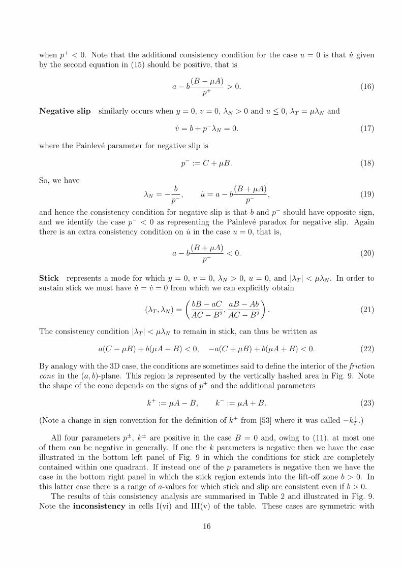
All four parameters p±, k± are positive in the case B = 0 and, owing to (11), at most oneof them can be negative in generally. If one the k parameters is negative then we have the caseillustrated in the bottom left panel of Fig. 9 in which the conditions for stick are completelycontained within one quadrant. If instead one of the p parameters is negative then we have thecase in the bottom right panel in which the stick region extends into the lift-off zone b > 0. Inthis latter case there is a range of a-values for which stick and slip are consistent even if b > 0.

The results of this consistency analysis are summarised in Table 2 and illustrated in Fig. 9.Note the inconsistency in cells I(vi) and III(v) of the table. These cases are symmetric with

16

Mode pos. Slip (S+) neg. Slip (S−) sTick (T ) lift ofF (F )kinematic ad-missibility

y = v = 0 and u ≥ 0 y = v = 0 and u ≤ 0 y = v = 0 andu = 0

y > 0; or y = 0and v ≥ 0

equality con-straints

λT = −µλN and v =0

λT = µλN and v = 0 u = v = 0 λN = λT = 0

consistency λN ≥ 0; and if u = 0:u > 0

λN ≥ 0; and if u = 0:u < 0

λN ≥ 0; and|λT | ≤ µλN

if y = v = 0:v > 0

Table 1: Constraints of the four contact modes.

Figure 9: Consistency regions of the four contact modes in the plane of parameters a and b atthree values of the coefficient of friction µ, for sustained contact y = v = 0 with positive tangentialvelocity (u > 0, top) and with stationary contact (u = 0, bottom). The case illustrated is forA = 1.1; B = 0.3; C = 0.1. The largest value of µ induces p+ < 0 for which there are regions ofindeterminacy and inconsistency in the parameter plane.

17

I: u > 0 II: u = 0 III: u < 0(i): b > 0, p+ > 0, p− > 0 F F F(ii): b > 0, p+ > 0, p− < 0 F F or (F and T and S−) F and S−

(iii): b > 0, p+ < 0, p− > 0 F and S+ F or (F and T and S+) F(iv): b < 0, p+ > 0, p− > 0 S+ T or S+ or S− S−(v): b < 0, p+ > 0, p− < 0 S+ S+ or T —

(vi): b < 0, p+ < 0, p− > 0 — S− or T S−

Table 2: Consistency of the contact modes depending on the signs of b, u, p+, p−. Here ‘or’ isexclusive and which mode occurs depends on other inequality conditions between a, b, A, B andC; specifically, stick occurs if and only a and b lie in the interior of the friction cone given by(3.1). However ‘and’ is inclusive and represents indeterminacy. A ‘—’ symbol is used to denotecases where there is no consistent mode.

respect to each other under the transformation x → −x, B → −B, which maps forward tobackward slip, so without loss of generality we consider the case for positive slip; y = v = 0, b < 0p+ > 0, u > 0. Here, stick is not possible since u > 0, nor is lift-off into free motion, because thefree acceleration b is in the direction towards the constraint surface y = 0. Negative slip is notpossible because u > 0, and finally positive slip is not possible because λN given by (4) wouldbe negative. To resolve what must happen in such cases, in practice we need to consider thepossibility of an IWC, which will do in the next subsection.

There are also two different types of indeterminacy, comprising four cases in all. The firsttype is indeterminacy between slip and lift-off in cells I(iii) and III(ii), with these two cases beingsymmetric with respect to each other under the transformation that maps positive slip to negativeslip. So, without loss of generality, consider positive slip; that is y = v = 0, b > 0, p+ > 0, u > 0.Here, stick is not possible because u > 0 but lift off is possible, as is positive slip, with λNgiven by (4) being positive because it is the ratio of two negative quantities. The other type ofindeterminacy is between liftoff, stick and slip, in cells II(ii) and II(iii) where b > 0 and a is suchthat we lie inside the friction cone (that is, inside the multi-shaded region of the bottom-rightpanel of Fig. 9). Here lift-off is possible because b > 0. Additionally though, a positive normalforce λN can be found such that the conditions for stick are satisfied. In addition, a larger normalforce λN exists such that slip is possible for the direction corresponding to the parameter p± thatis negative. These cases of indeterminacy cannot be resolved in general (in the sense of Question1 in the introduction), but can be resolved in terms of their stability (in the sense of Question 2)see Sec. 4 below.

3.2 Impact

As discussed in Sec. 2.4, the discussion of the Painleve paradox in a rigid body framework requiresthe inclusion of an impact law. Indeed, if contact regularisation is included in the normal direction,the necessity of IWC is easily concluded (see e.g. [52]). Following [79, 53] we shall introduce aformalism for the impact phase as something occurring on an asymptotically faster timescale τ =t/ε in which contact forces become asymptotically large (|λT |, λN = O(ε−1)) such that velocities(u, v) (and more generally q) can vary by an O(1) amount, but the generalised coordinates q remainconstant. We shall introduce a notation that the pre- and post-impact velocities are representedusing superscripts − and + respectively.

18

Then, if we define the rescaled contact forces ΛT,N = ελT,N then from (8), (9) we get in

du

dτ= ΛTA+ ΛNB +O(ε), (24)

du

dτ= ΛTB + ΛNC +O(ε), (25)

where A, B and C are now constant during the impact process. Moreover, we can replace time τwith units of the normal impulse [79]

IN =

∫ΛNdτ

which is a monotonically increasing function of τ . Then we get

u′ = (ΛT/ΛN)A+B +O(ε),

v′ = (ΛT/ΛN)B + C +O(ε),

where a prime represents ddIN

. These equations, after substitution from the Coulomb friction law(2) with λT,N replaced by ΛT,N , lead to leading order to explicit affine equations for u(IN) andv(IN). In fact, as shown in [53], the motion is always along straight lines in the (u, v)-plane, withcorners occurring at transitions between slip and stick during the impact process; see Fig. 10 forexamples.

The impact process can then be defined as a composite mapping

(u−, v−) 7→compression phase (u∗, 0) 7→restitution phase (u+, v+), (26)

where in each of the compression and restitution phases one needs to account for possible tran-sitions from slip to stick. It is possible to then define a composite closed from expression for theimpact map under different combinations of the signs of p+, p−, k+ and k− defined in (13), (18)and (23), and different conditions on the ratio u−/v− between initial velocities. The results aresummarised in Fig. 10; detailed calculations under the assumption of an energetic impact law in[53]. In that case we deem an impact to be over when the normal kinetic energy gained duringrestitution is −r2 times the normal kinetic energy lost during compression. This defines an en-ergetic coefficient of restitution r = re. Similar calculations can be carried out explicitly for thePoisson impact law (see e.g. [13]), the only difference being the point at which the restitutionphase is deemed to be over. In that case, restitution is deemed to end when the normal impulsein IN =

∫ΛN gained during restitution is r times the normal impulse gained during compression,

which defines a Poisson coefficient of restitution r = rpNote that the assumption that the same Coulomb friction law should apply during the impact

phase as in the O(1)-timescale motion is a modelling assumption that doesn’t necessarily follow.For example, when modelling impact in a so-called superball, it has been suggested that a frictionlaw is used where the transition between stick and slip occurs not at u = 0 but for some non-zerou > 0 [14]. In truth, frictional forces are temperature, timescale and spacescale dependent, seee.g. [91]. The impact process (26) can in principle be defined under different friction laws, orindeed for a different value of the coefficient of friction µI than for the O(1)-timescale motion.

Note that in general v− < 0, but that in parameter regions 5(b) or 6(c) in the figure, the impactequations also have a solution if v− = 0. These regions correspond precisely to when either of thePainleve parameters p+ or p− is negative and the pre-impacting motion is in slip of the correct

19

Figure 10: After [53], reproduced with permission. Graphical description of the impact process,in: the typical case (a) p+, p−, k+, k− > 0; the Painleve cases (b) p+ < 0, (b) p− < 0; or the slipreversal cases (c) k− < 0, (d) k+ < 0. In each case the mapping is depicted from an incomingvelocity pair (u−, v−) with v− ≤ 0 to an outgoing pair (u+, v+) with v+ > 0. The dashedlines represent boundaries between regions in (u−, v−)-space, represented by a different numericalsymbols, in which the map takes a different functional form.

20

sign (u > 0 or u < 0 respectively). In particular these two parameter regions are precisely wherean impact can occur with v− = 0, that is an impact without collision. Note these cases map tothe inconsistent and the indeterminate cases of Table 2 with u 6= 0. Thus, we have at least oneforward solution in all cases.

Also note from the Fig. 10 that impact can result in the phenomenon of slip reversal, that iswhere u+u− < 0 so that the body will enter impact with slipping in one direction and exit slippingin the other. This phenomenon occurs in parameter regions 7-10 of the figure which occurs whenone of the parameters k+ or k− is negative.

3.3 Chattering and inverse chattering

Chattering, also known as the Zeno phenomenon, is the process by which an infinite sequenceof impacts occurs in a finite period of time. In single degree-of-freedom mechanical systems,such a sequence can easily occur whenever there is a coefficient of restitution less than unityand acceleration that is towards the contact for a sufficiently long period of time. The canonicalexample of such an impact sequence occurs when dropping an elastic ball on a rigid floor, andcan also occur in general impact oscillators, see [15, 56] and references therein. For systems withoblique impacts, chattering sequences can also converge in reverse time.

To understand this phenomenon, following [55] we define a chattering sequence as a rapidsequence of impacts interspersed with brief intervals of free flight. To analyse such a sequence, weconsider a single iterate that starts immediately prior to the nth impact, as defined in the previoussection, and ends immediately prior to the (n+ 1)st impact. This defines a bounce mapping

g :

(u−nv−n

)7→impact map i

(u+nv+n

)7→free flight map f

(u−n+1

v−n+1

). (27)

Now, it is easy to see that for chatter to occur at all we need the free normal acceleration tobe towards the contact, that is b < 0. Moreover, we assume that the impact we are analysing issufficiently far into the sequence that the normal velocities are small. Then the time spent in freeflight is

tn = −2(v+n /b) +O[(v+n )2]. (28)

Therefore we can write the free flight map, up to order (v+n )2 as

f :

(u+nv−n

)7→(u+n − (2a/b)v+n

−v+n

),

and define an effective normal coefficient of restitution via the ratio

e :=v−n+1

v−n. (29)

Note that because v−n+1 = −v+n this ratio e is precisely the Newtonian coefficient of restitution,which ignores the motion in the tangential direction.

If e < 1 then we have a chattering sequence that accumulates as n→∞, and the times of flighttn represent a geometric sequence, whose sum converges to a finite limit which is proportional to(1−e)−1. In the context of impact oscillators this process is sometimes called a complete chatteringsequence (see [15, Ch.6] and references therein); in the context of hybrid systems, the limit point ofthis process is sometimes called a Zeno point (see e.g. [40]). The process is like that of a bouncing

21

ball coming to rest in finite time. For non-oblique impacts (i.e. when B = 0) it is possible to showthat e = r, a property that still holds true whenever there are no transitions from slip to stickduring the impact process (in regions 1,2 of Fig. 10).

However, Nordmark et al [55] show that under situations where there is a transition fromslip to stick during impact, then it is possible to find configurations such that e > 1, even ifthe energetic coefficient r < 1. This seems paradoxical. If the impact process itself cannot gainenergy, then how can a chattering sequence occur such that the normal velocity increases frominfinitesimal values to finite ones? The resolution is that the bounce map in this case represents aprocess by which energy is being scavenged from the tangential degree of freedom and transferredto the normal degree of freedom, such that total energy is still dissipated by a factor r2e in eachbounce.

The case e > 1 gives the possibility of reverse chatter [55]. That is, where the sequence definedby the bounce mapping g converges as n → −∞. Note that such a situation would lead to anextreme form of indeterminacy. We would have an infinite sequence of increasing bounces thatstarts at some time t0 with zero displacement and an arbitrary phase. This arbitrary constant getsmultiplied by a factor e > 1 at each bounce, so that at an O(1)-time later there are a continuum ofdifferent possible solutions, separated in phase by the finite time interval tn, given by (28). Sincetn → 0 as n → −∞ in this case, we find that trajectories for all these different phases emergefrom the same initial condition. Fig. 11(c),(d) illustrates the phenomenon.

The paper [55] enumerates carefully the cases for which reverse chatter is possible; the resultsare summarised in Fig. 11(a),(b). Note that it is not a necessary condition that we are in thePainleve region. In particular, panel (b) illustrates the conditions for e > 1 for the CPP, and herereverse chatter can be triggered all the way down to µ = 0 in the case of perfectly elastic collisionsr = 1.

3.4 Stability

Most forms of motion within rigid-body systems with contact can be described by special solutions(e.g. equilibria, limit cycles or invariant sets) of an appropriately defined dynamical system. Inorder to understand which of these motions may be observed in practice, it is common to examinethe stability of these solutions. There are however several notions of stability in dynamical systems,and the choice of an appropriate definition is made more subtle by the presence of unilateralconstraints. Fundamentally though, to define stability we really need to understand two things;what kind of motion is being considered as being stable, and what kind of perturbations shouldwe be stable against.

The simplest kind of motion is equilibrium. Equilibrium configurations in contact only existif every contact is in stick. We shall consider the case of multiple contact points in Sec. 6.For the present we shall confine ourselves to configurations with a single point of contact. Onecharacterisation of stability of an equilibrium in stick contact is that the the system should resistsmall variations of external forces. The difficulty of such a definition is that such forces are notusually considered as states of the system, rather as external inputs or parameters. Qualitativeinvariance of the state of a dynamical system under changes to inputs or parameters is sometimesreferred to as robustness (or roughness) of the system, or more general to structural stability ratherthan dynamic stability. Stability to changes in external forces is sometimes therefore studied bycontact regularisation, in which a (large) finite contact stiffness is introduced, so that a changein force necessarily implies a change in the system state. Contact regularisation in the normaldirection forms the subject of Sec. 4 below.

22

a

¡b

pp

¹

r = 1

decreasing r

¹

µ

r = 1

r = 0

(a) (b)

(c)vv

(d)

Figure 11: Reproduced from [55], with permission. (a) The region in a/(−b) and µ, for fixedB = 0.5, C = A = 1 and various r-values, for which e > 1. The region for which reverse chatteris possible is to the right of the curve depicted for each r-value. The case r = 0.7 leads to theshaded region. Note in this case that the Painleve region p+ < 0 is given by µ > 2. (b) The sameplot for the specific case of the CPP (1) in terms of the angle θ. Here the region above each curvefor fixed r represents where there exists a range of θ-values for which reverse chatter is possible.(c),(d) Simulation of a reverse chatter event in the equations for a falling rod with applied bodyforces, using a stiff compliant model in which the penetration y is allowed to be violated as in(30), see [55] for the details.

23

More generally, for systems with rigid contact, we can distinguish between normal stabilityand tangential stability, depending on whether we allow state perturbations at contact pointsthat have components in the normal direction or not. Normal stability requires stability againstthe possibility of lift-off or impact, whereas tangential stability presumes that contact is alwaysmaintained. The study of the former generally requires normal contact regularisation, whereastangent stability can be conducted using Filippov theory [20], without the need to introduce extracompliance.

The key question in tangential stability is whether general motion in stick (not just restrictedto equilibria) can be unstable to perturbations that would cause slip. This question is consideredin [55, Sec. 3] for the 2D single-contact case. It is shown that provided p± > 0 and the contactis in interior of the friction cone, then stick (with u = 0) represents a stable sliding manifold inthe sense of Filippov (see also [15]). Thus, motion in stick in case II(iv) of Table 2 is stable toperturbations with u 6= 0 except at the boundary of the friction cone where a straightforwardtransition into either positive or negative slip occurs (depending on which edge of the frictioncone is in question). A more subtle argument needs to be used in the case that stick occurs in oneof the Painleve parameter regions (in cells II(ii),(iii),(v) or (vi)). In [55, Sec. 3] it is shown that ifstick is normally stable then a posteriori it can be shown that stick is must also be tangentiallystable in the sense of Filippov.

Upon consideration of a larger class of state perturbations than just small variations of externalforces, the most widely used notion of stability is that of Lyapunov stability, that any smallperturbation should remain bounded. A yet stronger condition is asymptotic stability, namelythat such perturbations should also decay exponentially. Equilibria involving frictional systemsrarely possess asymptotic stability, because dry friction tends to create continuous equilibriumsets, and perturbations typically push the system to a nearby point within the set [44]. Thusit is natural to discuss Lyapunov stability in the context of rigid-body systems with contact.In the robotics community, the concept of strong stability has been proposed to refer to a casewhere stick is the only consistent mode with u = 0 at each contact (see [64] and Sec. 6.4 belowfor further discussion). Or and Rimon [58] refer to such a property as unambiguity and showthat it is a necessary condition for Lyapunov stability of a stick equilibrium. We propose here ageneralisation of Or and Rimon’s result to stipulate necessary and sufficient condition for Lyapunovstability for an equilibrium in the presence of any conservative external loads and a single pointcontact. Specifically, three conditions must be met:

1. The curvatures of the object and the contact surface must ensure a local minimum of thepotential energy of external forces along trajectories within stick (the T mode). If thiscriterion is not met, divergence from the equilibrium with the T mode becomes possible.

2. The equilibrium must be unambiguous in the sense of [58]. Unambiguity ensures that thesystem may not diverge from the equilibrium state in F , S+ or S− modes unless it undergoesand impact.

3. Additionally, upon defining the effective restitution coefficient e for chatter as in (29), thenwe must have e < 1. Otherwise a small perturbation may trigger diverging reverse-chattermotion.

Analogous conditions in the multi-contact case will be discussed in Sec. 6.4

24

4 Resolution of paradoxes via contact regularisation

Returning to Table 2, we can see that Question 1 can be resolved in the inconsistent regionsby the requirement that an IWC must occur. This leaves the indeterminate regions. We shallnow analyse these cases in the sense of Question 3, by adopting contact regularisation, that is,introduction of a form of finite elasticity into the model and then passing to the limit that thestiffness tends to infinity. There are a number of different choices that can be made. For example,Neimark and Smirnova [52] propose including both normal and tangential compliance. However,as argued in the previous section, unlike normal stability, tangential stability can be analysedwithout the need to introduce compliance. Therefore the simplest approach, adopted here, is tointroduce compliance in the normal direction only, and otherwise assume that the assumptionsof rigid body mechanics occur, including Coulomb friction. A good general discussion of normalcompliance can be found in the book by Anh [4].

It is useful though to point out a promising alternative approach due to Szalai [82, 81], whointroduced a formulation that models the response of a compliant surface through a delay kernel.In unpublished work, Berdeni [7] applies this approach to the Painleve paradox. By taking thefast wavespeed limit, a regularisation occurs via additional continuous degrees of freedom for thenormal and tangential forces.

Following Nordmark et al [55], we replace the rigid constraint y ≥ 0 by an assumption thatthere can be small O(ε) excursions into y < 0, where ε > 0 is a small parameter. Furthermore, wesuppose that the normal force is given by a specific expression

λN(y, v) =

{0 for y ≥ 0, v ≥ 0 ,

fN(y, v) otherwise,(30)

where y = ε−1y; v = dy/dt; t = ε−1/2t. Note that the timescale associated with contact is O(ε1/2),which explains the scaling of variables. We suppose that the restoring force has the followingproperties:

1. fN is continuous and fN(0, 0) = 0 so that λN is also continuous, and fN → 0 as y → +∞

2. fN is also smooth (at least of class C1) whenever fN > 0,

3. fN is restoring, that is∂fN∂y

< 0 for fN > 0,

4. fN is dissipative∂fN∂v

< 0 for fN > 0.

Such assumptions are essentially equivalent to replacing the normal rigid contact with a (possiblynonlinear) spring and damper in parallel that reach the rigid limit as ε→ 0. Moreover, it is alsopossible to choose the specific function fN such that it relaxes to a (Poisson or energetic) impactlaw as ε→ 0.

25

4.1 Normal stability of free fall

The free fall mode does not involve active contacts, i.e. λN = λT = 0. The fact that the contactforces are zero makes them robust against small perturbations. That is if y > 0 then smallperturbations in normal force cannot affect the motion. Alternatively, free motion can occur ify = 0 and v > 0. Here small perturbation of normal force will not be sufficient to make v = 0.Hence the system remains in F mode in response to small perturbation, which means that we canconsider the F mode to be normally stable.

4.2 Normal stability of stick

Introducing the definition (30) into the formulation (8), (9) and assuming the conditions for stickapply, then we have an equilibrium solution in the y-direction for which, according to (4.2),

λN = λ0N =aB − AbAC −B2

> 0

and hence we have an equilibrium penetration y0 < 0 corresponding to stick. Now let

y = y0 + y, λN = λ0N + λN := fN(y0, 0) + ky + qv + o(y, v),

where

k =∂fN∂y

∣∣∣∣(y0,0)

q =∂fN∂v

∣∣∣∣(y0,0)

.

are well defined, by property 3 above. Substituting these expressions into (8) and (9), to leadingorder we obtain

d

dt

[yv

]=

[0 1Kk Kq

] [yv

],

where

K =aB − AbAC −B2

> 0.

Note, from properties 1 to 4 above, that k < 0 and q < 0. Hence the 2 × 2 matrix has twoeigenvalues with negative real part. We conclude that the equilibrium y = y0 is normally stable.Taking the limit ε → 0, we conclude that stick is normally stable. Note that although y0 → 0in this limit, the normal force λ0N remains finite. So in force space, the T mode is not close tothe F mode and so stick remains stable against small perturbations. However, the asymptoticstability occurs on the fast time-scale t and so as we pass to the limit ε→ 0, the normal Lyapunovexponent tends to −∞.

Thus, upon the introduction of compliance and taking the infinite stiffness limit, a firm con-clusion can be made within cells II(ii) and II(iii) of Table 2. That is, if a body is in the stateof sustained stick, then this motion is stable to small perturbations in forces and the only wayto leave sticking is by reaching the boundary of the friction cone. In particular, a body that isin contact and sticking will remain in stick, even if the Painleve region with b > 0 is reached,provided that the body remains inside the friction cone.

26

I: u > 0 II: u = 0 III: u < 0(i): b > 0, p+ > 0, p− > 0 F F F(ii): b > 0, p+ > 0, p− < 0 F F or (F and T ) F and IWC

(iii): b > 0, p+ < 0, p− > 0 F and IWC F or (F and T ) F(iv): b < 0, p+ > 0, p− > 0 S+ T or S+ or S− S−(v): b < 0, p+ > 0, p− < 0 S+ S+ or T IWC

(vi): b < 0, p+ < 0, p− > 0 IWC S− or T S−

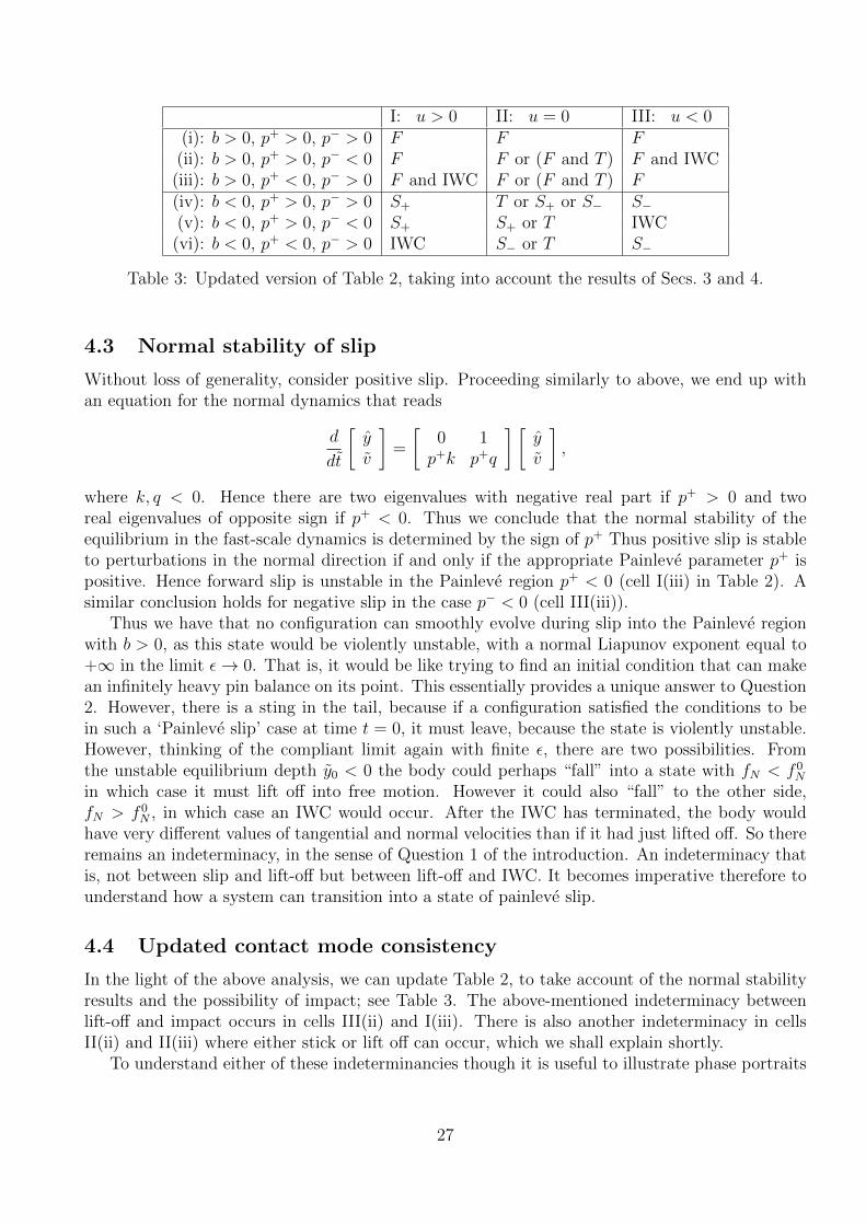
Table 3: Updated version of Table 2, taking into account the results of Secs. 3 and 4.

4.3 Normal stability of slip

Without loss of generality, consider positive slip. Proceeding similarly to above, we end up withan equation for the normal dynamics that reads

d

dt

[yv

]=

[0 1p+k p+q

] [yv

],

where k, q < 0. Hence there are two eigenvalues with negative real part if p+ > 0 and tworeal eigenvalues of opposite sign if p+ < 0. Thus we conclude that the normal stability of theequilibrium in the fast-scale dynamics is determined by the sign of p+ Thus positive slip is stableto perturbations in the normal direction if and only if the appropriate Painleve parameter p+ ispositive. Hence forward slip is unstable in the Painleve region p+ < 0 (cell I(iii) in Table 2). Asimilar conclusion holds for negative slip in the case p− < 0 (cell III(iii)).

Thus we have that no configuration can smoothly evolve during slip into the Painleve regionwith b > 0, as this state would be violently unstable, with a normal Liapunov exponent equal to+∞ in the limit ε→ 0. That is, it would be like trying to find an initial condition that can makean infinitely heavy pin balance on its point. This essentially provides a unique answer to Question2. However, there is a sting in the tail, because if a configuration satisfied the conditions to bein such a ‘Painleve slip’ case at time t = 0, it must leave, because the state is violently unstable.However, thinking of the compliant limit again with finite ε, there are two possibilities. Fromthe unstable equilibrium depth y0 < 0 the body could perhaps “fall” into a state with fN < f 0

N

in which case it must lift off into free motion. However it could also “fall” to the other side,fN > f 0

N , in which case an IWC would occur. After the IWC has terminated, the body wouldhave very different values of tangential and normal velocities than if it had just lifted off. So thereremains an indeterminacy, in the sense of Question 1 of the introduction. An indeterminacy thatis, not between slip and lift-off but between lift-off and IWC. It becomes imperative therefore tounderstand how a system can transition into a state of painleve slip.

4.4 Updated contact mode consistency

In the light of the above analysis, we can update Table 2, to take account of the normal stabilityresults and the possibility of impact; see Table 3. The above-mentioned indeterminacy betweenlift-off and impact occurs in cells III(ii) and I(iii). There is also another indeterminacy in cellsII(ii) and II(iii) where either stick or lift off can occur, which we shall explain shortly.

To understand either of these indeterminancies though it is useful to illustrate phase portraits

27

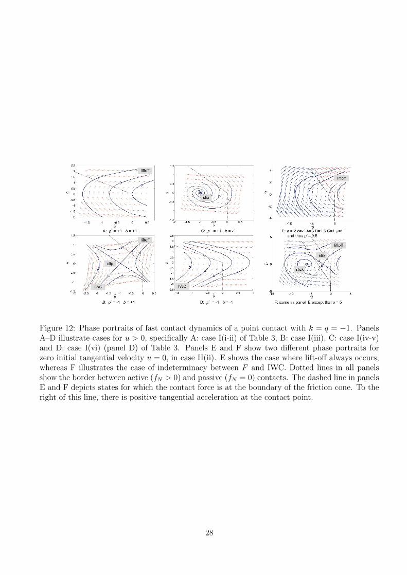
Figure 12: Phase portraits of fast contact dynamics of a point contact with k = q = −1. PanelsA–D illustrate cases for u > 0, specifically A: case I(i-ii) of Table 3, B: case I(iii), C: case I(iv-v)and D: case I(vi) (panel D) of Table 3. Panels E and F show two different phase portraits forzero initial tangential velocity u = 0, in case II(ii). E shows the case where lift-off always occurs,whereas F illustrates the case of indeterminacy between F and IWC. Dotted lines in all panelsshow the border between active (fN > 0) and passive (fN = 0) contacts. The dashed line in panelsE and F depicts states for which the contact force is at the boundary of the friction cone. To theright of this line, there is positive tangential acceleration at the contact point.

28

of the regularised contact dynamics. See Fig. 12, in which we have used (30) with

fN = max

[ky + qv

0

](31)

where k and q are negative scalars.Consider first cases where the initial condition is in slip and, without loss of generality, let

us assume u > 0. The four possible cases are illustrated in Fig. 12(A-D). If b < 0 < p+ (caseI(iv)) then the normal dynamics has a globally attractive equilibrium corresponding to positiveslip. In contrast, if b > 0 > p+ (case I(iii)) the positive slip normal equilibrium corresponds to asaddle point, and trajectories converge to y = +∞ (liftoff) or y = −∞ (IWC) depending on initialconditions. In the remaining two cases, slipping was found inconsistent in Sec. 3. Accordingly thedynamics of the compliant contacts has no equilibrium and every trajectory converges to y = +∞if 0 < b, p+, or to y = −∞ if 0 > b, p+. This picture confirms the result that the contact undergoesliftoff in case I(i) and IWC in case I(iv).

Consider now initial conditions for which u = 0. Then in all cases other than II(ii-iii), phaseportraits like Fig. 12(A) or (C) occur where now the normal equilibrium corresponds to stick ratherthan slip if the equilibrium is in the interior of the friction cone. Fig. 12(E) and (F) illustrate thepossibly indeterminate case II(iii) (case II(ii) is similar). Panel E represents the case where theconfiguration (ignoring normal compliance) is outside of the friction cone and the only possibilityis motion in F mode. Here a dashed line shows those states for which zero tangential accelerationrequires λT = −µλN . To the left of this line, the contact remains in stick, whereas to the rightof this line it has positive tangential acceleration so that slip or lift-off must occur. Crossingfrom left to right corresponds to a stick-slip transition, whereas crossing from right to left doesnot represent a transition because u > 0. These latter trajectories do not follow the depicted(sticking) vector field as long as the tangential velocity of the contact point remains positive; onesuch trajectory is depicted by a dot-dashed line. Nevertheless we see in this case that all initialconditions eventually lead to lift-off, and so F remains the only mode.

Fig. 12(F) illustrates the other branch of the “or” in cell II(iii) of Table 2 in which thereare additional feasible T and S+ modes. Here we see that the T mode represents a stable focuswhereas slipping S+ can be seen to be a saddle point, and hence unstable, in accordance with thecalculations in Secs. 4.2 and 3.3 above. Note though that there is still indeterminacy in this case,because lift off (mode F ) is another possibility, which is represented here by trajectories divergingto positive infinity in y. Note that the stable manifold of the saddle separates trajectories thatare attracted to mode T from those which lift-off.

5 Triggered transitions between states

In this section we focus on Question 2, namely what are the generic ways in which a configurationcan enter a Painleve region and what must then happen. Theoretically, there are only two ways ofreaching sustained contact in a Painleve state; (1) moving from non-Painleve contact to Painlevecontact, or (2) establishing sustained contact via the termination of a chattering sequence, insidethe Painleve regime. We deal with these two possibilities in the next two subsections. We shallthen look at ways in which reverse chatter may be triggered while in contact.

29

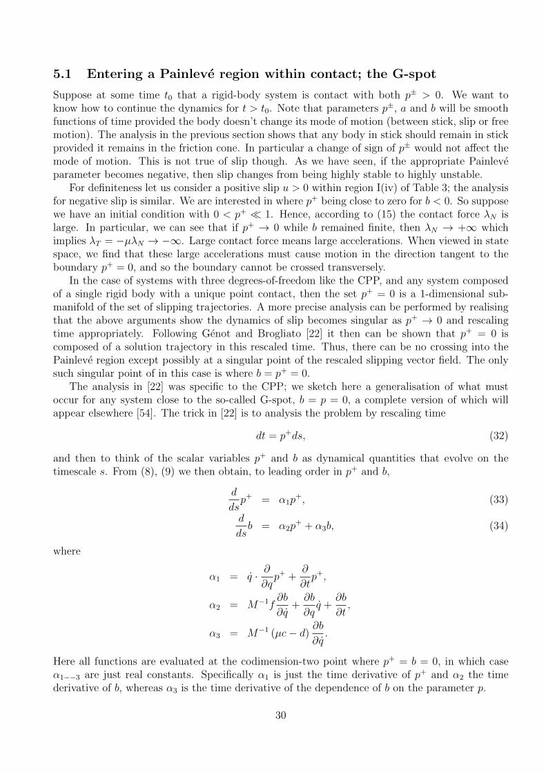
5.1 Entering a Painleve region within contact; the G-spot

Suppose at some time t0 that a rigid-body system is contact with both p± > 0. We want toknow how to continue the dynamics for t > t0. Note that parameters p±, a and b will be smoothfunctions of time provided the body doesn’t change its mode of motion (between stick, slip or freemotion). The analysis in the previous section shows that any body in stick should remain in stickprovided it remains in the friction cone. In particular a change of sign of p± would not affect themode of motion. This is not true of slip though. As we have seen, if the appropriate Painleveparameter becomes negative, then slip changes from being highly stable to highly unstable.

For definiteness let us consider a positive slip u > 0 within region I(iv) of Table 3; the analysisfor negative slip is similar. We are interested in where p+ being close to zero for b < 0. So supposewe have an initial condition with 0 < p+ � 1. Hence, according to (15) the contact force λN islarge. In particular, we can see that if p+ → 0 while b remained finite, then λN → +∞ whichimplies λT = −µλN → −∞. Large contact force means large accelerations. When viewed in statespace, we find that these large accelerations must cause motion in the direction tangent to theboundary p+ = 0, and so the boundary cannot be crossed transversely.

In the case of systems with three degrees-of-freedom like the CPP, and any system composedof a single rigid body with a unique point contact, then the set p+ = 0 is a 1-dimensional sub-manifold of the set of slipping trajectories. A more precise analysis can be performed by realisingthat the above arguments show the dynamics of slip becomes singular as p+ → 0 and rescalingtime appropriately. Following Genot and Brogliato [22] it then can be shown that p+ = 0 iscomposed of a solution trajectory in this rescaled time. Thus, there can be no crossing into thePainleve region except possibly at a singular point of the rescaled slipping vector field. The onlysuch singular point of in this case is where b = p+ = 0.

The analysis in [22] was specific to the CPP; we sketch here a generalisation of what mustoccur for any system close to the so-called G-spot, b = p = 0, a complete version of which willappear elsewhere [54]. The trick in [22] is to analysis the problem by rescaling time

dt = p+ds, (32)

and then to think of the scalar variables p+ and b as dynamical quantities that evolve on thetimescale s. From (8), (9) we then obtain, to leading order in p+ and b,

d

dsp+ = α1p

+, (33)

d

dsb = α2p

+ + α3b, (34)

where

α1 = q · ∂∂qp+ +

∂

∂tp+,

α2 = M−1f∂b

∂q+∂b

∂qq +

∂b

∂t,

α3 = M−1 (µc− d)∂b

∂q.

Here all functions are evaluated at the codimension-two point where p+ = b = 0, in which caseα1−−3 are just real constants. Specifically α1 is just the time derivative of p+ and α2 the timederivative of b, whereas α3 is the time derivative of the dependence of b on the parameter p.

30

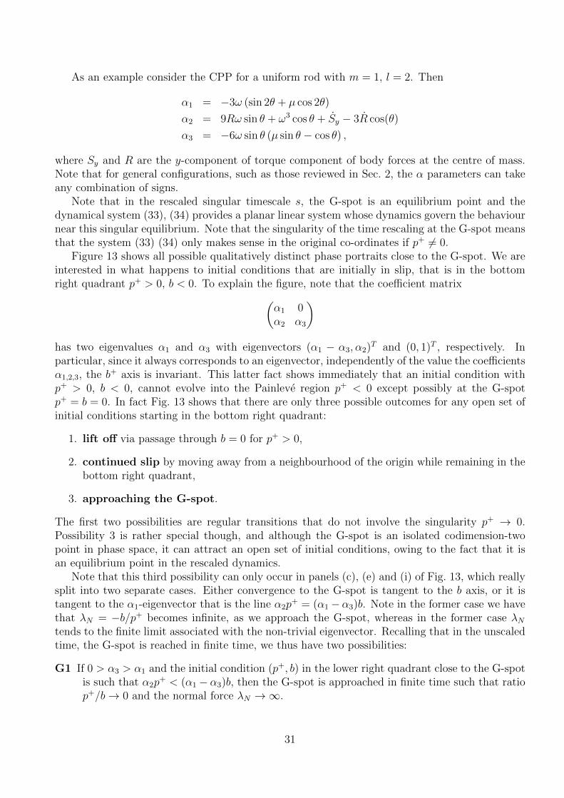
As an example consider the CPP for a uniform rod with m = 1, l = 2. Then

α1 = −3ω (sin 2θ + µ cos 2θ)

α2 = 9Rω sin θ + ω3 cos θ + Sy − 3R cos(θ)

α3 = −6ω sin θ (µ sin θ − cos θ) ,

where Sy and R are the y-component of torque component of body forces at the centre of mass.Note that for general configurations, such as those reviewed in Sec. 2, the α parameters can takeany combination of signs.

Note that in the rescaled singular timescale s, the G-spot is an equilibrium point and thedynamical system (33), (34) provides a planar linear system whose dynamics govern the behaviournear this singular equilibrium. Note that the singularity of the time rescaling at the G-spot meansthat the system (33) (34) only makes sense in the original co-ordinates if p+ 6= 0.

Figure 13 shows all possible qualitatively distinct phase portraits close to the G-spot. We areinterested in what happens to initial conditions that are initially in slip, that is in the bottomright quadrant p+ > 0, b < 0. To explain the figure, note that the coefficient matrix(

α1 0α2 α3

)has two eigenvalues α1 and α3 with eigenvectors (α1 − α3, α2)

T and (0, 1)T , respectively. Inparticular, since it always corresponds to an eigenvector, independently of the value the coefficientsα1,2,3, the b+ axis is invariant. This latter fact shows immediately that an initial condition withp+ > 0, b < 0, cannot evolve into the Painleve region p+ < 0 except possibly at the G-spotp+ = b = 0. In fact Fig. 13 shows that there are only three possible outcomes for any open set ofinitial conditions starting in the bottom right quadrant:

1. lift off via passage through b = 0 for p+ > 0,

2. continued slip by moving away from a neighbourhood of the origin while remaining in thebottom right quadrant,

3. approaching the G-spot.

The first two possibilities are regular transitions that do not involve the singularity p+ → 0.Possibility 3 is rather special though, and although the G-spot is an isolated codimension-twopoint in phase space, it can attract an open set of initial conditions, owing to the fact that it isan equilibrium point in the rescaled dynamics.

Note that this third possibility can only occur in panels (c), (e) and (i) of Fig. 13, which reallysplit into two separate cases. Either convergence to the G-spot is tangent to the b axis, or it istangent to the α1-eigenvector that is the line α2p

+ = (α1−α3)b. Note in the former case we havethat λN = −b/p+ becomes infinite, as we approach the G-spot, whereas in the former case λNtends to the finite limit associated with the non-trivial eigenvector. Recalling that in the unscaledtime, the G-spot is reached in finite time, we thus have two possibilities:

G1 If 0 > α3 > α1 and the initial condition (p+, b) in the lower right quadrant close to the G-spotis such that α2p

+ < (α1− α3)b, then the G-spot is approached in finite time such that ratiop+/b→ 0 and the normal force λN →∞.

31

C ¡ ¹B

b

C ¡ ¹B

b

C ¡ ¹B

b

C ¡ ¹B

b

C ¡ ¹B

b

C ¡ ¹B

b

C ¡ ¹B

b

C ¡ ¹B

b

C ¡ ¹B

b

C ¡ ¹B

b

C ¡ ¹B

b

C ¡ ¹B

b

®2 < 0

®3 > ®1 > 0

®1 > ®3 > 0

®2 > 0 ®2 > 0

®1 > 0 > ®3

®3 > 0 > ®1

®2 < 0

0 > ®1 > ®3

®2 > 0

0 > ®3 > ®1

®2 < 0

®2 < 0

®1 > 0 > ®3

®2 < 0

0 > ®1 > ®3

®2 < 0

®1 > ®3 > 0

®2 > 0

®3 > ®1 > 0

®2 > 0

®3 > 0 > ®1

®2 > 0

0 > ®3 > ®1

Figure 13: Reproduced from [54]. Analysis of the dynamics of the neighbourhood of the G-spot.In each panel, the phase plane of (33), (34) is depicted, for all possible sign combinations of theparameters α1,2,3. Here the bold line passing through the origin represents the location of thesecond eigenvector, and the arrows on this line and the b-axis represent whether each represents astable or unstable manifold. In the case of a two-dimensional stable (unstable) eigenspace, doublearrows are used to represent the strong stable (unstable) manifold. The dashed line represents thelocation of the horizontal nullcline. Arrows crossing this line and also the (C − µB)-axis indicatethe direction of solution trajectories there

32

G2 If α2 < 0, 0 < α1 < α3 then the G-spot is approached in finite time, and λN approaches thefinite limit α2/(α3 − α1) > 0.

Each of these cases correspond to what has been referred to in the literature as dynamic jam.What happens next beyond dynamic jam remains an open question. In principle after the G-spot,there could be an IWC, a lift off event or even possibly a velocity jump immediately into stick(recall that u > 0 as we approach the G-spot). It seems that these possibilities cannot easily bedistinguished using the contact regularisation approach of Sec. 4.

5.2 Reaching a Painleve state via complete chatter

The analysis in Secs. 3 and 4 analyse both stick and slip in the Painleve regions, assuming thata trajectory arrived in the Painleve state by smooth evolution while in contact. We found thatstick is unaffected by either p± < 0, provided the body is in the interior of the friction cone. Incontrast, the analysis in Sec. 5.1 above shows that the only way to enter the Painleve region whileslipping is via the G-spot. What we have not investigated though is whether a complete chattersequence can end up a Zeno point that is in the Painleve region.

In order for a chattering sequence to occur, we must have b < 0. Hence the indeterminate casesof stick (cells II(ii) and III(ii) in Table 3) cannot be reached. So, consider instead the possibilityof slip. Suppose that the parameter p+ < 0 and consider the possibility of a chattering sequenceleading to positive slip. Here, we are in the case of impact mappings as depicted in Fig. 10(b).Note that any impact with an initial velocity with u− > 0, must end up with u+ = 0. Similarlyany impact with u− < 0 ends up with u+ ≤ 0. Hence the only possibility is that the Zeno pointhas u ≤ 0. But note that there is no inconsistency or indeterminacy in this case (see cells I(vi)and II(vi) in Table 3). We either get stick or negative slip, the latter of which is consistent becausep− > 0.

A similar conclusion holds if p− < 0, we cannot approach the Painleve region for negative slipas the result of a chattering sequence. We conclude that even if one of the parameters p± < 0, itis not possible to have a Zeno point in the Painleve region, thus dismissing this is a possible routeinto the Painleve region.

5.3 Triggering reverse chatter

A final possibility for a complex triggered transition would be if a body that is smoothly in contact,were to spontaneously undergo a reverse chatter sequence. This possibility was considered byNordmark et al [55], the results of which we summarise here.

In general, we can rule out such a spontaneous triggering of reverese chatter in T mode bythe analysis of Sec. 4.2 since, provided the body remains in the interior of the friction cone, stickis stable. Similarly, the analysis of Sec. 4.3 rules out the possibility of spontaneous triggering ofreverse chatter from within a condition of sustained slip, as this is stable wherever it is consistent(unless the border of Painleve-ness is crossed, which was shown to be impossible). Similarly,reverse chatter cannot be triggered at the end of a forward chattering sequence, because such asequence necessarily converges to a point where e < 1.

This leaves the possibility that reverse chatter can be triggered at the boundary of one of thecontact phases, namely at the termination of stick, or of slip. But, an analysis of the cases wheree can be greater than one shows that these are necessarily a subset of the cases that are in theinterior of the friction cone. Hence it can be concluded that reverse chatter can only be triggered

33

at the end of a slip phase. Then, it can be argued that either a case of stick is triggered, or undercertain other conditions, in addition to e > 1, we might get the triggering of reverse chatter.

Nordmark et al [55] enumerate the details and find that there are further inequality conditionson a, b, A, B, C, µ and r that determine whether reverse chatter can be triggered from a transitioninto stick. Then they show, by introducing a compliant model, as in Sec. 4, that if these conditionsare satisfied then the situation is not uniformly resolvable. That is, the precise details of thecompliant force fN can affect whether regular stick motion of reverse chatter is triggered. We areleft with another indeterminate case.

6 Multiple contact points

Let us now consider generalisation of the previous results to systems with multiple contacts. Oneaim is to identify which properties of Painleve’s paradox are generally true, and which are specificproperties of single-contact systems. Moreover, we will uncover many extra forms of degeneracythat are unique to multiple-contact point systems.

One of the main difficulties with answering Question 1 is that if we allow F , T , S+ and S− ateach of n contacts, then this induces 4n possible contact modes (although some of them will bekinematically inadmissible). This combinatorial complexity makes a consistency check for eachpotential combination computationally unfeasible for large n. In what follows we therefore focusmostly on the simplest case of just two frictional contacts.

Ivanov [32] considered generalisations of the CPP for a rod that has two points of contactswith rough rigid surfaces under the assumption that each contact undergoes slip. He enumeratedthe conditions under which the Painleve paradox appears for suitably chosen external forces. Theclassification scheme of Ivanov has recently been refined by Varkonyi [84] to the level of ouranalysis in Sec. 3.1. A summary of and commentary on these results appear in the next threesubsections.

6.1 Consistency analysis of contact modes

To begin with, consider a planar rigid-body system that has two point contacts, with nonzerotangential velocities: xi = yi = vi = 0 and ui > 0 for i = 1, 2. Thus there are four kinematicallyadmissible modes: S+S+, S+F , FS+, and FF . Here the two-letter symbols refer to the specificcombination of modes at the two contacts. The contact forces and accelerations are determinedwith the help of the equality constraints of Table 2 for both contacts. A contact mode is deemedconsistent, if the consistency conditions of Table 2 are satisfied for both contacts.

The key observation is that the general analytical expressions for contact motion in Sec. 3 stillapply, specifically the equation (14), but where now b and λN are vectors in R2 and p+ is a matrixof size 2 × 2. In this formulation, the elements p+ij of p+ represent the normal acceleration ofcontact i in response to a slipping contact force with a normal component of unit size at contactj.

Varkonyi [84] has recently enumerated all the consistent modes under this restriction of nosticking modes. In order to summarise the results of his analysis, it is convenient to introducethe following notation. Let pj represent the jth column vector of p+ such that p+ = [p1 p2].Furthermore, let γj be the angle between pj and vector [1 0]T . For example, if pj = [0 1]T thenγj = π/2. Similarly, we let γj be the angle between −pj and the vector [1 0]T and β be theangle between −b and [1 0]T . It can be shown that the consistency of each contact mode can be

34

Classes Contact modes IWCname (dual) FF S+S+ S+F FS+ IF FI II11 (self) 5 2 1 2 6 2 3 412 (self) 5 2 1 6 3 413 (41) 5 2 3 1 6 414 (31) 4 5 2 3 4 1 6 4 (x)15 (32) 4 5 1 5 6 1 6 4 (x)16 (21) 4 1 6 1 5 6 4 5 x22 (45) 5 3 4 5 3 4 x23 (46) 5 3 3 4 5 4 x24 (36) 4 5 3 4 3 4 5 4 x (x)25 (self) 4 3 4 5 3 4 4 5 x x (x)26 (self) 4 1 2 6 3 4 4 5 x x33 (44) 4 5 3 4 5 3 (x)34 (self) 3 4 5 4 5 3 (x)35 (self) 3 4 5 4 4 5 3 4 (x)42 (self) 4 1 2 6 5 343 (self) 4 3 4 5 5 3 (x)

Table 4: Classification of planar systems with two non-sticking contacts. See text for details.

determined using a string of three integers

s1s2s3, where s1 ∈ {1, 2, 3, 4}, s2,3 ∈ {1, 2, . . . 6},

which code the relative position of the vectors p1, p2, b and the co-ordinate axes. Specificallythe index s1 represents the quadrant of R2 that contains p1. Equivalently, s1 is the index of theinterval among the four ordered intervals [0, π/2], [π/2, π], [π, 3π/2], [3π/2, 2π] that contains γ1.In a similar fashion, the second integer s2 represents the index of the interval among the set ofordered closed intervals bounded by 0, γ1, γ1 π/2, π, 3π/2 and 2π that contains γ2. The finalinteger s3 represents the index of the interval among the set of ordered closed intervals boundedby 0, γ1, γ2 π/2, π 3π/2 and 2π that contains β.

The relative positions of the vectors p1, p2 and b corresponding to each class of configurationsis depicted in Fig. 6.1. Thus, for example, the upper right panel refers to classes 14s3 wheres3 = 1, 2, 3 . . . 6. Here we see, according to the above notation, that s1 = 1 and so p1 is in the firstquadrant. In addition, s2 = 4 and so p2 is in third quadrant with positive angle to the [0 1]T axisthat is less than that of −p1. The s3-value corresponding to possible locations of b are indicatedby dashed arrows, which depicts the relative position of the vector b with respect to p1, p2 andthe four co-ordinate semi-axes.

The results of the consistency analysis are summarised in Table 4. To cut down the numberof rows of the table and sub-panels of Fig. 6.1, we have used the fact that each class has a dualthat is obtained by swapping the labels of contact 1 and contact 2. This corresponds to swappingthe labels p1 and p2 and reflecting both vectors in the line 45◦ line in each case. The dual classs1s2 of each of the depicted cases s1s2 is given in brackets in the first column of Table 4, includingcases that are self-dual. Note that the first two digits s1s2 of any class represents the coarserclassification of Ivanov [32]. The last digit s3 refines the classification into subclasses within whichthe consistency of each contact mode becomes uniquely determined (as depicted in columns 2 to

35

Figure 14: Relative positions of the vectors p1 and p2 (solid arrows) and the four co-ordinatesemi-axes in each class s1s2. In each case, every possible position of the third vector b, whichdelineates the third integer s3 is indicated by a dashed arrow. Note that only one member of eachdual pair of classes is displayed, see Table 4 for the corresponding dual s1s1 in each case.

36

5 of the table). The significance of the shading of these columns and the meaning of the last threecolumns will be explained in the next subsection.

Note already that there are multiple occurrences of indeterminacy and inconsistency indicatedin the table. For example, within class 15, subclasses 151, 154 and 156 are indeterminate becausetwo contact modes in each case are consistent. In contrast subclasses 152 and 153 are inconsistentbecause there is no consistent contact mode for these cases. There are also several examples oftriple indeterminacy, for example in subclass 112 where S+S+ and S+F and FS+ are all consistentand of quadruple indeterminacy where all four possible contact modes are consistent, for examplein subclasses 254 or 354.

Before going on to look at normal stability of these modes and the possibility of impact, itis worth stressing that Table 4 is only a partial classification for two contacts, because it ignoresstick and cases where negative and positive slip can simulateously occur at different contacts.As far as the authors know, a general classification is not yet known, nor is a classification incases where there are more than two contacts. Nevertheless, other examples of indeterminacy areknown. Two such cases were illustrated in Fig. 7. The left-hand panel depicts a case in whichthe static equilibrium represents the TT mode which is consistent provided there is a sufficientlylarge friction force at the contacts (solid arrows in the figure show the gravitational force and apossible choice of reaction forces). Simultaneously, the FF mode is also consistent, in which casethe block will just fall. The right-hand panel of Fig. 7 illustrates a shape resting on a slope inwhich both the body may be in equilibrium in mode TT , but for which motion in mode S+F isalso consistent.

6.2 Contact regularisation and stability analysis

To resolve the indeterminate cases, we can compute the normal stability of different kinds ofcontact via the method introduced in Sec. 4. That is, we introduce a contact regularisation in thenormal direction, linearise the ensuing equations of motion, perform an eigenvalue analysis on theappropriate Jacobian matrix and then pass to the infinite stiffness limit.

Applying this methodology to the cases enumerated in Table 4, it is straightforward to see thata contact in mode F does not influence the normal stability. Hence, the stability analysis of theS+F and FS+ contact modes is identical to the analysis of S+ in Sec. 4. Specifically, we obtainthat S+F is stable if p11 > 0 and FS+ is stable if p22 > 0. For the S+S+ mode, the simultaneousdynamics of two contacts is described by a system of four first-order ODEs, and thus normalstability analysis requires the study of eigenvalues of a 4× 4 Jacobian matrix. The Jacobian andthus the stability properties of contact modes are independent of b. Hence the same results areobtained for all subclasses within this class.

The results of the stability analysis are summarised in Table 4. Details of the calculationsare presented in [84]. Stability information is indicated by shading of the appropriate cell in thetable. A dark (grey) shading indicates definitely unstable. Lighter (yellow, colour online) shadingrepresents where the S+S+ mode may be stable, depending on further conditions. Finally, noshading represents a normally stable situation. One interesting thing to note is that the stabilityof the S+S+ mode is not uniquely determined in classes 13, 41, 14, 31, 23 and 46. The unstableregions within these subclasses are caused by so-called mode coupling – a phenomenon studied inthe context of break squeal (see e.g. [30, 27]). In these regions, a system may cross the stabilityboundary during its motion. In such a situation, a spontaneous contact mode transition will occur.That is, the system would switch from the S+S+ mode to a different type of motion, despite thefact that the S+S+ mode remains consistent. As we argued in Secs. 3 and 4 such spontaneous

37

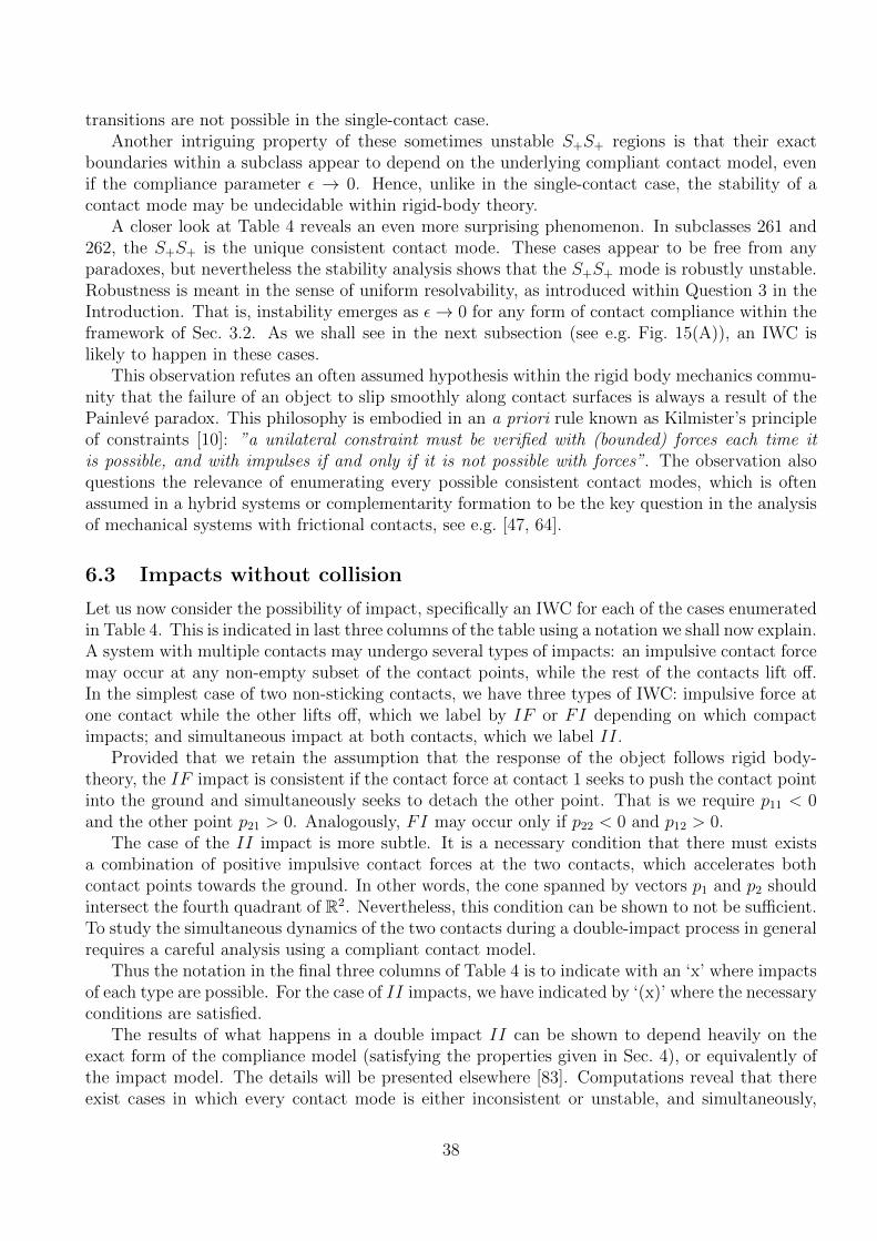
transitions are not possible in the single-contact case.Another intriguing property of these sometimes unstable S+S+ regions is that their exact

boundaries within a subclass appear to depend on the underlying compliant contact model, evenif the compliance parameter ε → 0. Hence, unlike in the single-contact case, the stability of acontact mode may be undecidable within rigid-body theory.

A closer look at Table 4 reveals an even more surprising phenomenon. In subclasses 261 and262, the S+S+ is the unique consistent contact mode. These cases appear to be free from anyparadoxes, but nevertheless the stability analysis shows that the S+S+ mode is robustly unstable.Robustness is meant in the sense of uniform resolvability, as introduced within Question 3 in theIntroduction. That is, instability emerges as ε→ 0 for any form of contact compliance within theframework of Sec. 3.2. As we shall see in the next subsection (see e.g. Fig. 15(A)), an IWC islikely to happen in these cases.

This observation refutes an often assumed hypothesis within the rigid body mechanics commu-nity that the failure of an object to slip smoothly along contact surfaces is always a result of thePainleve paradox. This philosophy is embodied in an a priori rule known as Kilmister’s principleof constraints [10]: ”a unilateral constraint must be verified with (bounded) forces each time itis possible, and with impulses if and only if it is not possible with forces”. The observation alsoquestions the relevance of enumerating every possible consistent contact modes, which is oftenassumed in a hybrid systems or complementarity formation to be the key question in the analysisof mechanical systems with frictional contacts, see e.g. [47, 64].

6.3 Impacts without collision

Let us now consider the possibility of impact, specifically an IWC for each of the cases enumeratedin Table 4. This is indicated in last three columns of the table using a notation we shall now explain.A system with multiple contacts may undergo several types of impacts: an impulsive contact forcemay occur at any non-empty subset of the contact points, while the rest of the contacts lift off.In the simplest case of two non-sticking contacts, we have three types of IWC: impulsive force atone contact while the other lifts off, which we label by IF or FI depending on which compactimpacts; and simultaneous impact at both contacts, which we label II.

Provided that we retain the assumption that the response of the object follows rigid body-theory, the IF impact is consistent if the contact force at contact 1 seeks to push the contact pointinto the ground and simultaneously seeks to detach the other point. That is we require p11 < 0and the other point p21 > 0. Analogously, FI may occur only if p22 < 0 and p12 > 0.

The case of the II impact is more subtle. It is a necessary condition that there must existsa combination of positive impulsive contact forces at the two contacts, which accelerates bothcontact points towards the ground. In other words, the cone spanned by vectors p1 and p2 shouldintersect the fourth quadrant of R2. Nevertheless, this condition can be shown to not be sufficient.To study the simultaneous dynamics of the two contacts during a double-impact process in generalrequires a careful analysis using a compliant contact model.

Thus the notation in the final three columns of Table 4 is to indicate with an ‘x’ where impactsof each type are possible. For the case of II impacts, we have indicated by ‘(x)’ where the necessaryconditions are satisfied.

The results of what happens in a double impact II can be shown to depend heavily on theexact form of the compliance model (satisfying the properties given in Sec. 4), or equivalently ofthe impact model. The details will be presented elsewhere [83]. Computations reveal that thereexist cases in which every contact mode is either inconsistent or unstable, and simultaneously,

38

Figure 15: Simulation of fast contact dynamics in examples of (A) class 261 and (B) class 142using the contact model (31). See text for details. The corresponding panels (C) and (D) showpossible configurations that display the dynamics in panels (A) and (B) respectively. Parametervalues used are (A) a = [1 1]T , B = [[−0.055 0.055]T [0.088 − 0.036]T ], inducing γ1 = 0.75π;γ2 = 1.875π; α = 0.25π, and (B) a = [1 0.727]T , B = [[3.051 1.555]T [−1.677 − 0.0375]T ], k1 = 1;k2 = 3; q1 = q2 = 1.2, inducing γ1 = 0.15π; γ2 = 1.07π; and α = 0.2π.

the three forms of IWC mentioned above are impossible, see Fig. 15(B). This observation pointstowards the incorrectness of another common assumption: that Painleve’s paradox is perfectlyresolvable by considering IWCs.

Figure 15(A) shows a planar projection of the phase portrait of the fast contact dynamics for aconfiguration within class 261 (where the S+S+ mode is the unique consistent contact mode, butit is unstable, see Sec. 6.2). Several different initial conditions are depicted in which the initialtime derivatives of yi are 0. The contact model (31) is used in the simulation, with k = q = −1.For every possible initial condition, one of the two contact penetrations, and hence the normalforce diverges to minus infinity. The other contact always lifts off. In the rigid limit ε → 0 thisbehaviour corresponds to an IWC at one of the two contacts, and lift off at the other, that is,either mode IF or mode FI. Note that the contact dynamics also has a consistent mode S+S+

in which both contacts slip, marked by a square in the figure, but this is unstable. The stablemanifold of this point in the fast dynamics represents the dividing surface between two differenttypes of IWC.

Figure 15(B) shows an example within class 142 in which there is the onset of some kind ofmicro-scale sprag-slip oscillation. Here there is also an unstable S+S+ mode, again represented bya square. For the parameter values depicted, every other contact mode is inconsistent and IWCs

39

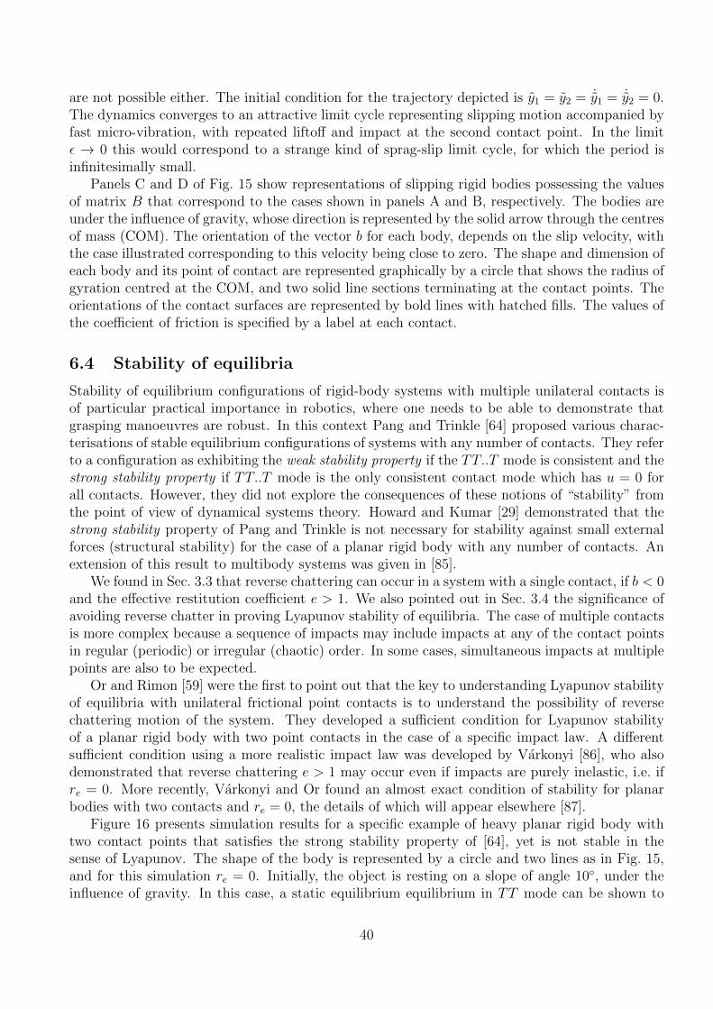
are not possible either. The initial condition for the trajectory depicted is y1 = y2 = ˙y1 = ˙y2 = 0.The dynamics converges to an attractive limit cycle representing slipping motion accompanied byfast micro-vibration, with repeated liftoff and impact at the second contact point. In the limitε → 0 this would correspond to a strange kind of sprag-slip limit cycle, for which the period isinfinitesimally small.

Panels C and D of Fig. 15 show representations of slipping rigid bodies possessing the valuesof matrix B that correspond to the cases shown in panels A and B, respectively. The bodies areunder the influence of gravity, whose direction is represented by the solid arrow through the centresof mass (COM). The orientation of the vector b for each body, depends on the slip velocity, withthe case illustrated corresponding to this velocity being close to zero. The shape and dimension ofeach body and its point of contact are represented graphically by a circle that shows the radius ofgyration centred at the COM, and two solid line sections terminating at the contact points. Theorientations of the contact surfaces are represented by bold lines with hatched fills. The values ofthe coefficient of friction is specified by a label at each contact.

6.4 Stability of equilibria

Stability of equilibrium configurations of rigid-body systems with multiple unilateral contacts isof particular practical importance in robotics, where one needs to be able to demonstrate thatgrasping manoeuvres are robust. In this context Pang and Trinkle [64] proposed various charac-terisations of stable equilibrium configurations of systems with any number of contacts. They referto a configuration as exhibiting the weak stability property if the TT..T mode is consistent and thestrong stability property if TT..T mode is the only consistent contact mode which has u = 0 forall contacts. However, they did not explore the consequences of these notions of “stability” fromthe point of view of dynamical systems theory. Howard and Kumar [29] demonstrated that thestrong stability property of Pang and Trinkle is not necessary for stability against small externalforces (structural stability) for the case of a planar rigid body with any number of contacts. Anextension of this result to multibody systems was given in [85].

We found in Sec. 3.3 that reverse chattering can occur in a system with a single contact, if b < 0and the effective restitution coefficient e > 1. We also pointed out in Sec. 3.4 the significance ofavoiding reverse chatter in proving Lyapunov stability of equilibria. The case of multiple contactsis more complex because a sequence of impacts may include impacts at any of the contact pointsin regular (periodic) or irregular (chaotic) order. In some cases, simultaneous impacts at multiplepoints are also to be expected.

Or and Rimon [59] were the first to point out that the key to understanding Lyapunov stabilityof equilibria with unilateral frictional point contacts is to understand the possibility of reversechattering motion of the system. They developed a sufficient condition for Lyapunov stabilityof a planar rigid body with two point contacts in the case of a specific impact law. A differentsufficient condition using a more realistic impact law was developed by Varkonyi [86], who alsodemonstrated that reverse chattering e > 1 may occur even if impacts are purely inelastic, i.e. ifre = 0. More recently, Varkonyi and Or found an almost exact condition of stability for planarbodies with two contacts and re = 0, the details of which will appear elsewhere [87].

Figure 16 presents simulation results for a specific example of heavy planar rigid body withtwo contact points that satisfies the strong stability property of [64], yet is not stable in thesense of Lyapunov. The shape of the body is represented by a circle and two lines as in Fig. 15,and for this simulation re = 0. Initially, the object is resting on a slope of angle 10◦, under theinfluence of gravity. In this case, a static equilibrium equilibrium in TT mode can be shown to

40

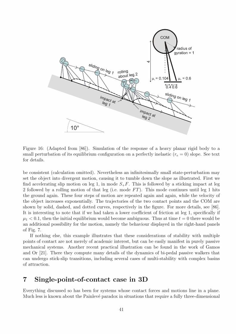
Figure 16: (Adapted from [86]). Simulation of the response of a heavy planar rigid body to asmall perturbation of its equilibrium configuration on a perfectly inelastic (re = 0) slope. See textfor details.

be consistent (calculation omitted). Nevertheless an infinitesimally small state-perturbation mayset the object into divergent motion, causing it to tumble down the slope as illustrated. First wefind accelerating slip motion on leg 1, in mode S+F . This is followed by a sticking impact at leg2 followed by a rolling motion of that leg (i.e. mode FT ). This mode continues until leg 1 hitsthe ground again. These four steps of motion are repeated again and again, while the velocity ofthe object increases exponentially. The trajectories of the two contact points and the COM areshown by solid, dashed, and dotted curves, respectively in the figure. For more details, see [86].It is interesting to note that if we had taken a lower coefficient of friction at leg 1, specifically ifµ1 < 0.1, then the initial equilibrium would become ambiguous. Thus at time t = 0 there would bean additional possibility for the motion, namely the behaviour displayed in the right-hand panelsof Fig. 7.

If nothing else, this example illustrates that these considerations of stability with multiplepoints of contact are not merely of academic interest, but can be easily manifest in purely passivemechanical systems. Another recent practical illustration can be found in the work of Gamosand Or [21]. There they compute many details of the dynamics of bi-pedal passive walkers thatcan undergo stick-slip transitions, including several cases of multi-stability with complex basinsof attraction.

7 Single-point-of-contact case in 3D

Everything discussed so has been for systems whose contact forces and motions line in a plane.Much less is known about the Painleve paradox in situations that require a fully three-dimensional

41

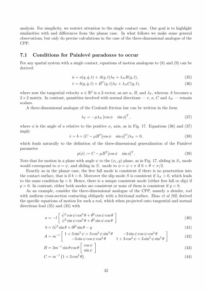
analysis. For simplicity, we restrict attention to the single contact case. Our goal is to highlightsimilarities with and differences from the planar case. In what follows we make some generalobservations, but only do precise calculations in the case of the three-dimensional analogue of theCPP.

7.1 Conditions for Painleve paradoxes to occur

For any spatial system with a single contact, equations of motion analogous to (8) and (9) can bederived:

u = a(q, q, t) + A(q, t)λT + λNB(q, t), (35)

v = b(q, q, t) +BT (q, t)λT + λNC(q, t), (36)

where now the tangential velocity u ∈ R2 is a 2-vector, as are a, B, and λT , whereas A becomes a2× 2 matrix. In contrast, quantities involved with normal directions — v, a, C and λN — remainscalars.

A three-dimensional analogue of the Coulomb friction law can be written in the form

λT = −µλN [cosφ sinφ]T , (37)

where φ is the angle of u relative to the positive x1 axis, as in Fig. 17. Equations (36) and (37)imply

v = b+ (C − µBT [cosφ sinφ]T )λN = 0, (38)

which leads naturally to the definition of the three-dimensional generalisation of the Painleveparameter

p(φ) := C − µBT [cosφ sinφ]T . (39)

Note that for motion in a plane with angle ψ to the (x1, y) plane, as in Fig. 17, sliding in S+ modewould correspond to φ = ψ, and sliding in S− mode to φ = ψ + π if 0 < θ < π/2.

Exactly as in the planar case, the free fall mode is consistent if there is no penetration intothe contact surface, that is if b > 0. Moreover the slip mode S is consistent if λN > 0, which leadsto the same condition bp < 0. Hence, there is a unique consistent mode (either free fall or slip) ifp > 0. In contrast, either both modes are consistent or none of them is consistent if p < 0.

As an example, consider the three-dimensional analogue of the CPP, namely a slender, rodwith uniform cross-section contacting obliquely with a frictional surface. Zhao et al [92] derivedthe specific equations of motion for such a rod, which when projected onto tangential and normaldirections lead (35) and (35) with

a = −l[ψ2 cosψ cos3 θ + θ2 cosψ cos θ

ψ2 sinψ cos3 θ + θ2 sinψ cos θ

](40)

b = lψ2 sin θ + lθ2 sin θ − g (41)

A = m−1[

1 + 3 sin2 ψ + 3 cos2 ψ sin2 θ −3 sinψ cosψ cos2 θ−3 sinψ cosψ cos2 θ 1 + 3 cos2 ψ + 3 sin2 ψ sin2 θ

](42)

B = 3m−1 sin θ cos θ

[cosψsinψ

](43)

C = m−1(1 + 3 cos2 θ

). (44)

42

Figure 17: left: a slender, three-dimensional rod slipping on a horizontal surface. The coordinateaxes x1 and x2 are horizontal, whereas axis y is vertical. Here u and u are the velocity and theacceleration of the contact point, respectively. Right: simulated trajectories of the slipping rod ina three-dimensional projection of state space, with the boundary of the Painleve region representedby the grey surface. Circles denote initial points of the trajectories and x-shaped markers indicatepoints of crossing p = 0. Parameter values used are µ = 1 and radius of gyration = 0.1l

Here, m is the mass and l is the half-length of the rod, θ is the angle between the rod and thehorizontal plane. The vectors u and λT are expressed in a global (x1, x2) reference frame, seeFig. 17.

Let us consider the possibility of the Painleve paradox for this problem. With the help of(41),(43), (44), the condition p < 0 for the Painleve paradox to occur can be expressed as

µ cos(φ− ψ) > µp(θ) =1 + 3 cos2 θ

3 cos θ sin θ, (45)

which is identical to the condition for the planar rod (5) if φ = ψ. Thus the Painleve paradox forthe 3D slender rod cannot occur if µ ≤ µP (θ) or if cos(φ− ψ) ≤ 0. In the case of µ ≥ µP (θ) theparadox occurs in a range of slip directions parametrised by φ−ψ ∈ (φmin, φmax), where φmax = 0if µ = µP (θ) and φmax grows to π/2 if µ→∞.

It was also shown in [92] that if the rod is in the Painleve regime with b < 0, the non-existenceparadox (inconsistency) can be resolved by assuming an IWC. This assumption was also justifiedby taking a compliant contact model similar in fashion to the one introduced in Sec. 4. To obtaina more detailed picture of the dynamics in the Painleve regime, Shen [72] considered a elasticfinite element model of the CPP, using a 3D rod of a finite thickness with a rounded end. He wasable to compare the dynamics during planar motion of the system in its plane of symmetry to thedynamics of an equivalent point contact model with a compliant contact point. He also arguedthat both models show that the continuation in the Painleve regime can be understood in termsof an IWC.

7.2 Dynamic jam

So far, we have not uncovered any behaviour of 3D systems that is qualitatively different from theplanar case, in terms of consistent contact modes or the emergence of IWC. However, when we

43

consider Question 2 from the introduction we get a more subtle answer. In particular, we foundin Sec. 5.1, that it was not possible to enter the Painleve region through the set p+ = 0 whileslipping, except at the G-spot where b is simultaneously zero. As we shall now show, this neednot be the case for 3D systems.

A fundamental difference that distinguishes the 2D and 3D cases is that for planar systems,the Painleve parameters p+ and p− depend on position variables q and coefficient of friction only.Whereas, note from (39) that p(φ) in general depends additionally on the generalised velocities q,through the definition of the angle φ. Note that the angle ψ is a cyclic coordinate of the slippingrod, hence we may assume ψ = 0 without loss of generality. Then, (35) can be expressed with thehelp of (40), (42), (43) and (37) as

mu = −l cos θ

[ψ2 cos2 θ + θ2

0

]− µλN

[1 + 3 sin2 θ 0

0 4

] [cosφsinφ

]+ 3 sin θ cos θλN

[10

](46)

Assume now that this system is very close to but outside of the Painleve regime, such that0 < p � 1. Furthermore, the free acceleration is such that the rod remains in contact (b < 0),which is the case, for example, if the rod has sufficiently small angular velocity. According to (38)we find that λN = −b/p � 1. Thus, O(1) terms in (46) become negligible in comparison withO(λN) terms, yielding

−mλ−1N · u = µ

[1 + 3 sin2 θ 0

0 4

] [cosφsinφ

]− 3 sin θ cos θ

[10

]+O(λ−1N )

= µ

[(1 + 3 sin2 θ)µ− 3 sin θ cos θ cos−1 φ 0

0 4µ

] [cosφsinφ

]+O(λ−1N ). (47)

The upper left element of the diagonal matrix in is smaller than the lower right one because

(1 + 3 sin2 θ)µ− 3 sin θ cos θ cos−1 φ ≤ (1 + 3)µ− 0 = 4µ. (48)

This means that the absolute value of the angle of the vector that −u makes relative to the positivex1 axis is larger than the absolute value of the angle φ of u. Therefore, φ approaches 0 over timein such a way that φ · sinφ < 0. Meanwhile the time derivative of the Painleve parameter p is (38)

p = C − d

dt

(µBT

)[cosφ sinφ]T − µBT d

dt[cosφ sinφ]T

in which all terms are O(1) except for the acceleration-like term ddt

[cosφ sinφ], which is O(λN).Neglecting the O(1) terms and substituting ψ = 0 leads to

p = −µBT d

dt[cosφ sinφ]T +O(1)

= 3µm−1 sin θ cos θ sinφφ+O(1),

which is negative because sinφφ < 0 and all other terms are positive. Thus we arrive to theconclusion that p becomes negative, and the system crosses the boundary of the Painleve regimetransversely away from the G-spot. Our conclusion is confirmed by numerical simulation (Fig. 17,right panel). What happens beyond this crossing is an open question.

44

8 Discussion

This article represents an attempt to survey the state of knowledge on the range complex phenom-ena in rigid body mechanics that have been grouped together under the epithet of the Painleveparadox. We have drawn particular attention to recent results by the authors and their collab-orators, while trying to establish some general notation and terminology that we hope will helpto organise the previous literature and stimulate other researchers to investigate this fascinatingtopic. Let us close with some philosophical remarks and a brief summary of open problems.

8.1 Philosophical remarks

Far from being resolved, the Painleve paradox on the inconsistency of rigid body mechanics withfrictional contact, first posed over 120 years ago, would seem to retain many open facets. Evenfor the highly restrictive situation of a planar configuration with a single point contact, we haveargued that there remain situations that are undecidable within the framework of rigid bodymechanics. In particular, slender bodies such as the classical Painleve problem of the falling rodreach a point of dynamic jam, from which it is not currently clear whether there is a uniqueforward continuation without including additional physics. In three dimensions, we have shownthat things are even worse, because the rod can enter the unstable Painleve region transversely.Here, the results in Table 3 suggest there is indeterminacy because the rod could lift-off or takean impact. Also, even outside the Painleve region, we argued in Sec. 5 that reverse chatter canbe triggered at a transition into stick. If reverse chatter occurs then there is infinite degeneracybetween a continuum of different phases. Nevertheless, for the single contact case in 2D we showedthat inclusion of an impact law and an analysis using contact regularisation enables resolution ofall inconsistent cases, but indeterminacy remains.

If one allows more than one contact point, then we indicated in Sec. 6 that there are many othercases of indeterminacy, and we have not yet been able to resolve all possible cases of inconsistency,even under the simplifying assumption that no contact is in stick. We have also provided evidence,for example through the micro-scale chatter-like behaviour of Fig. 15, that there may be far morecomplex possibilities for reverse or forward chatter-like behaviours in the case of two or morecontacts.

One thing that our analysis does point to though is the insufficiency of Kilmister’s principleapplied to rigid bodies with multiple contacts. That has led to a common approach in multibodymechanics to seek sufficient conditions under which there is a unique consistent contact mode,thus avoiding any Painleve paradoxes. We argue that this approach is misguided, because wealready know from the single point of contact case that there are easily reachable configurationsthat are inevitably undecidable and which cannot be resolved without breaking the assumptions ofrigid body mechanics. We also showed a specific case in Sec. 6 where there is a unique consistentcontact mode S+S+, but this is not normally stable and instead an IWC must occur. Ratherthan seek sufficient conditions to sweep the paradox under the carpet, as it were, we have beenmotivated instead by the three separate questions posed in the Introduction. In particular we haveattempted to separate the questions of: which configurations are consistent or determinate; howone may undergo a transition into an indeterminate state; and whether questions of consistencyor indeterminacy can be resolved by consideration of impact and contact regularisation.

Contact regularisation concerns the introduction of finite stiffnesses and in Sec. 4 we consideredonly the simplest kind, namely introduction of a stiffness in the normal degree of freedom. In onesense such normal regularisation can resolve all of the consequences of the Painleve paradoxes, if

45

one allows the stiffness to remain finite. Even in this case though, simple nonsmooth friction lawsin the tangent direction lead to Filippov systems which can themselves exhibit indeterminacy;see [34] for a mechanical example. The test we have used for genuine determinacy associatedwith the Painleve paradox is what we have termed uniform resolvability, namely that normalcontact regularisation leads to unique limiting behaviour in the infinite stiffness limit. If such aunique limit does not occur, such as in reverse chatter, then these cases we deem to be genuinelyindeterminate. Of course, there are many other possible approaches to regularisation, and wementioned already the approach of Szalai [82, 81] that appears promising.

We should also stress the fundamental point made in the Introduction that the Painleve para-dox is not about the real world, but an indication of the failure of rigid-body mechanics. Typicallyany friction or impact law is a gross approximation to tribological processes that occur at the mi-croscale. Thus, the existence of undecidability (either inconsistency or indeterminacy) within arigid body framework points to situations for which there will be extreme sensitivity with respectto initial conditions in the real mechanics.

An overarching conclusion then is that, for certain configurations at least, a purely rationalmechanics approach to rigid body dynamics with impact and friction is fundamentally ill-posed.To put it somewhat pejoratively, one might say that there is nothing “rational” about rationalmechanics at least for rigid bodies. There is a strong tradition going back to Newton, Euler andmany others in trying to discover the “laws of mechanics” and showing that they are consistent.This body of literature has become known as rational mechanics; and indeed the Archives forRational Mechanics and Analysis is one of the most prestigious scientific journals. The hope isthat one day, by posing sufficiently many constitutive laws one can come up with self-consistentcontinuum theories for fluids, elastic solids, elasto-plastic materials, etc. One of the simplest suchcontinuum theories is that of rigid body mechanics, which we typically teach to our studentsthrough an axiomatic approach. We talk about the Coulomb or Stribeck laws of friction, ratherthan models of friction. Nevertheless we have shown that with even the simplest consistent frictionand impact laws for contact with friction lead to fundamentally undecidable cases, and the searchfor a grand unifying law that resolves all cases is probably futile.

Rather like Russell & Whitehead’s attempt in Principia Mathematica [89] to systematise arith-metic and, by implication, the whole of mathematics (see, for example [28] for a popular account),we could argue that any mission with the aim rationalising rigid body mechanics through axiomsand laws is doomed to failure. Rather like the way Godel’s Incompleteness Theorem [23] showedthe impossibility of Russell and Whithead’s goal, in our view, the inconsistency and indeterminacythat is inherent in the Painleve paradox suggests that a complete, self-consistent, theory of rigidbody mechanics is impossible. It is also tempting to draw the analogy between Godel’s use ofparadox at the heart of his proof. If Godel’s work has taught us anything it is that no mathe-matical theory of sufficient complexity to describe the real work is ever complete; undecidabilityparadoxes are inevitable.

8.2 Open problems and perspectives

In Sec. 2.3 we reviewed some of the configurations that have been shown to exhibit Painleve para-dox phenomena. Many of the practical implications of the theory to these and related mechanismsremain unexplored. For example, is it possible to explain the transition to sprag-slip oscillationin brake-disc-like systems through a reverse chatter instability? Can such instabilities be used toexplain the mechanism for drawing dashed lines on a blackboard? Another practical area whichseems largely unexplored is in rotor machinery with contact, where there are large couplings be-

46

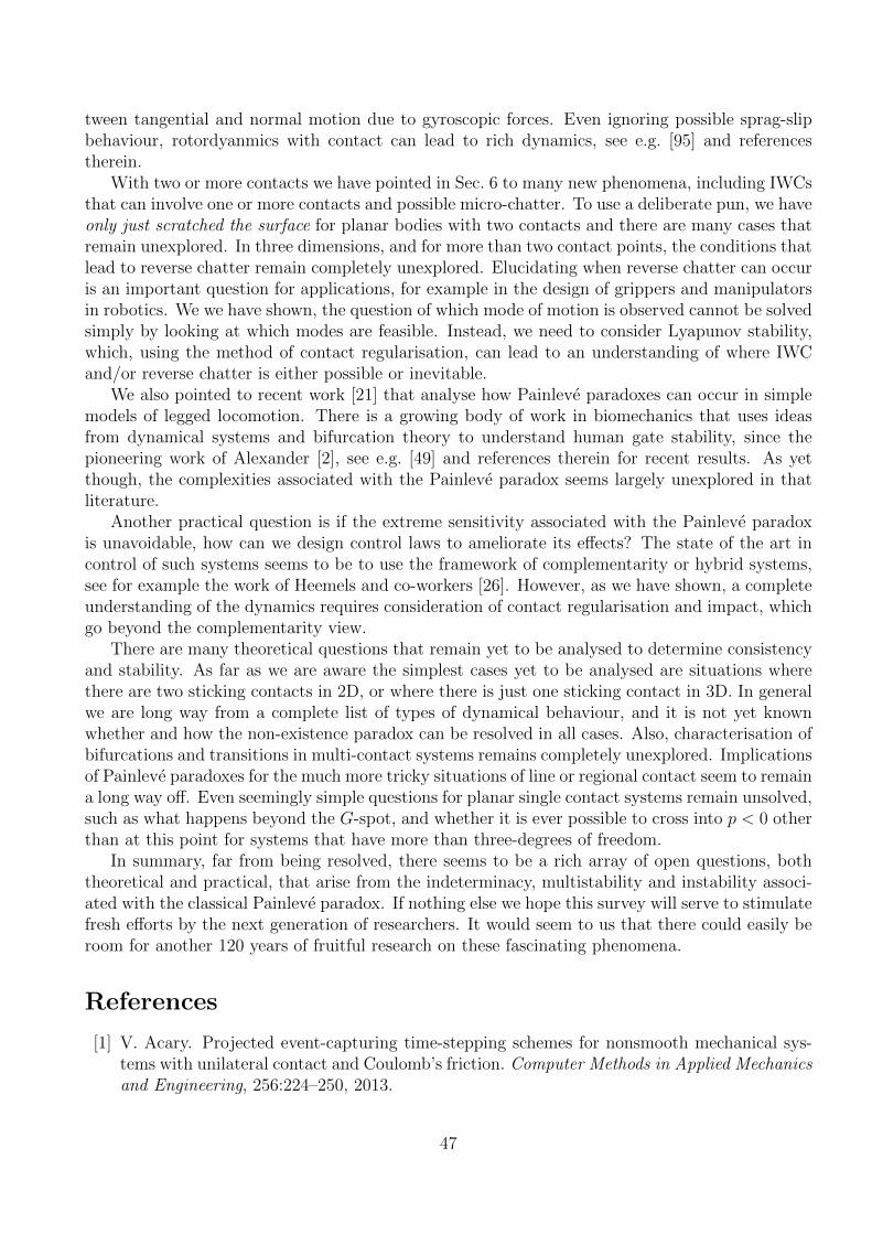
tween tangential and normal motion due to gyroscopic forces. Even ignoring possible sprag-slipbehaviour, rotordyanmics with contact can lead to rich dynamics, see e.g. [95] and referencestherein.

With two or more contacts we have pointed in Sec. 6 to many new phenomena, including IWCsthat can involve one or more contacts and possible micro-chatter. To use a deliberate pun, we haveonly just scratched the surface for planar bodies with two contacts and there are many cases thatremain unexplored. In three dimensions, and for more than two contact points, the conditions thatlead to reverse chatter remain completely unexplored. Elucidating when reverse chatter can occuris an important question for applications, for example in the design of grippers and manipulatorsin robotics. We we have shown, the question of which mode of motion is observed cannot be solvedsimply by looking at which modes are feasible. Instead, we need to consider Lyapunov stability,which, using the method of contact regularisation, can lead to an understanding of where IWCand/or reverse chatter is either possible or inevitable.

We also pointed to recent work [21] that analyse how Painleve paradoxes can occur in simplemodels of legged locomotion. There is a growing body of work in biomechanics that uses ideasfrom dynamical systems and bifurcation theory to understand human gate stability, since thepioneering work of Alexander [2], see e.g. [49] and references therein for recent results. As yetthough, the complexities associated with the Painleve paradox seems largely unexplored in thatliterature.

Another practical question is if the extreme sensitivity associated with the Painleve paradoxis unavoidable, how can we design control laws to ameliorate its effects? The state of the art incontrol of such systems seems to be to use the framework of complementarity or hybrid systems,see for example the work of Heemels and co-workers [26]. However, as we have shown, a completeunderstanding of the dynamics requires consideration of contact regularisation and impact, whichgo beyond the complementarity view.

There are many theoretical questions that remain yet to be analysed to determine consistencyand stability. As far as we are aware the simplest cases yet to be analysed are situations wherethere are two sticking contacts in 2D, or where there is just one sticking contact in 3D. In generalwe are long way from a complete list of types of dynamical behaviour, and it is not yet knownwhether and how the non-existence paradox can be resolved in all cases. Also, characterisation ofbifurcations and transitions in multi-contact systems remains completely unexplored. Implicationsof Painleve paradoxes for the much more tricky situations of line or regional contact seem to remaina long way off. Even seemingly simple questions for planar single contact systems remain unsolved,such as what happens beyond the G-spot, and whether it is ever possible to cross into p < 0 otherthan at this point for systems that have more than three-degrees of freedom.

In summary, far from being resolved, there seems to be a rich array of open questions, boththeoretical and practical, that arise from the indeterminacy, multistability and instability associ-ated with the classical Painleve paradox. If nothing else we hope this survey will serve to stimulatefresh efforts by the next generation of researchers. It would seem to us that there could easily beroom for another 120 years of fruitful research on these fascinating phenomena.

References

[1] V. Acary. Projected event-capturing time-stepping schemes for nonsmooth mechanical sys-tems with unilateral contact and Coulomb’s friction. Computer Methods in Applied Mechanicsand Engineering, 256:224–250, 2013.

47

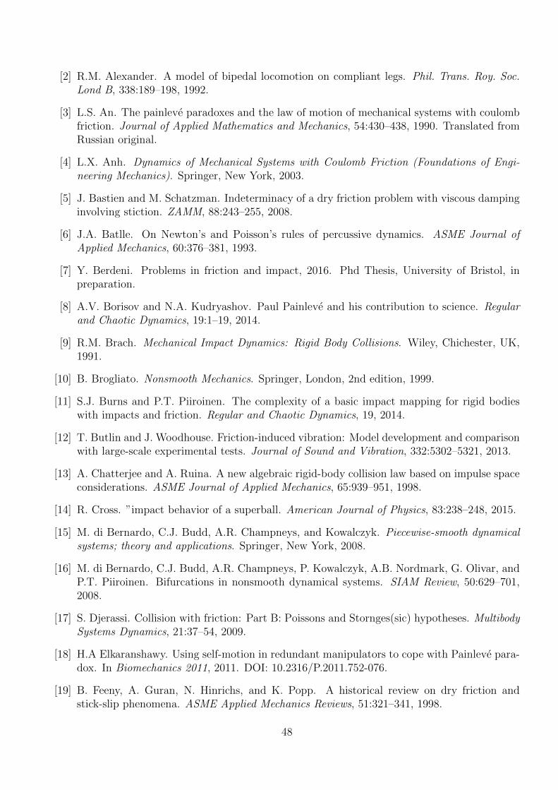
[2] R.M. Alexander. A model of bipedal locomotion on compliant legs. Phil. Trans. Roy. Soc.Lond B, 338:189–198, 1992.

[3] L.S. An. The painleve paradoxes and the law of motion of mechanical systems with coulombfriction. Journal of Applied Mathematics and Mechanics, 54:430–438, 1990. Translated fromRussian original.

[4] L.X. Anh. Dynamics of Mechanical Systems with Coulomb Friction (Foundations of Engi-neering Mechanics). Springer, New York, 2003.

[5] J. Bastien and M. Schatzman. Indeterminacy of a dry friction problem with viscous dampinginvolving stiction. ZAMM, 88:243–255, 2008.

[6] J.A. Batlle. On Newton’s and Poisson’s rules of percussive dynamics. ASME Journal ofApplied Mechanics, 60:376–381, 1993.

[7] Y. Berdeni. Problems in friction and impact, 2016. Phd Thesis, University of Bristol, inpreparation.

[8] A.V. Borisov and N.A. Kudryashov. Paul Painleve and his contribution to science. Regularand Chaotic Dynamics, 19:1–19, 2014.

[9] R.M. Brach. Mechanical Impact Dynamics: Rigid Body Collisions. Wiley, Chichester, UK,1991.

[10] B. Brogliato. Nonsmooth Mechanics. Springer, London, 2nd edition, 1999.

[11] S.J. Burns and P.T. Piiroinen. The complexity of a basic impact mapping for rigid bodieswith impacts and friction. Regular and Chaotic Dynamics, 19, 2014.

[12] T. Butlin and J. Woodhouse. Friction-induced vibration: Model development and comparisonwith large-scale experimental tests. Journal of Sound and Vibration, 332:5302–5321, 2013.

[13] A. Chatterjee and A. Ruina. A new algebraic rigid-body collision law based on impulse spaceconsiderations. ASME Journal of Applied Mechanics, 65:939–951, 1998.

[14] R. Cross. ”impact behavior of a superball. American Journal of Physics, 83:238–248, 2015.

[15] M. di Bernardo, C.J. Budd, A.R. Champneys, and Kowalczyk. Piecewise-smooth dynamicalsystems; theory and applications. Springer, New York, 2008.

[16] M. di Bernardo, C.J. Budd, A.R. Champneys, P. Kowalczyk, A.B. Nordmark, G. Olivar, andP.T. Piiroinen. Bifurcations in nonsmooth dynamical systems. SIAM Review, 50:629–701,2008.

[17] S. Djerassi. Collision with friction: Part B: Poissons and Stornges(sic) hypotheses. MultibodySystems Dynamics, 21:37–54, 2009.

[18] H.A Elkaranshawy. Using self-motion in redundant manipulators to cope with Painleve para-dox. In Biomechanics 2011, 2011. DOI: 10.2316/P.2011.752-076.

[19] B. Feeny, A. Guran, N. Hinrichs, and K. Popp. A historical review on dry friction andstick-slip phenomena. ASME Applied Mechanics Reviews, 51:321–341, 1998.

48

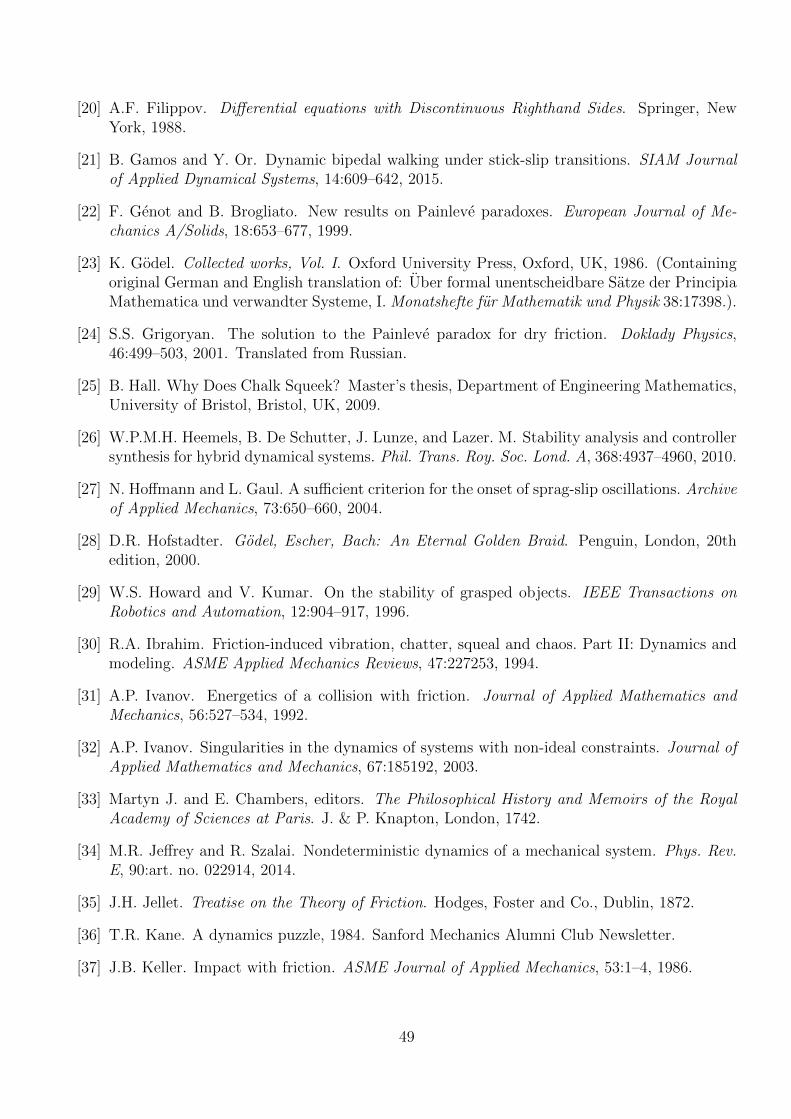
[20] A.F. Filippov. Differential equations with Discontinuous Righthand Sides. Springer, NewYork, 1988.

[21] B. Gamos and Y. Or. Dynamic bipedal walking under stick-slip transitions. SIAM Journalof Applied Dynamical Systems, 14:609–642, 2015.

[22] F. Genot and B. Brogliato. New results on Painleve paradoxes. European Journal of Me-chanics A/Solids, 18:653–677, 1999.

[23] K. Godel. Collected works, Vol. I. Oxford University Press, Oxford, UK, 1986. (Containingoriginal German and English translation of: Uber formal unentscheidbare Satze der PrincipiaMathematica und verwandter Systeme, I. Monatshefte fur Mathematik und Physik 38:17398.).

[24] S.S. Grigoryan. The solution to the Painleve paradox for dry friction. Doklady Physics,46:499–503, 2001. Translated from Russian.

[25] B. Hall. Why Does Chalk Squeek? Master’s thesis, Department of Engineering Mathematics,University of Bristol, Bristol, UK, 2009.

[26] W.P.M.H. Heemels, B. De Schutter, J. Lunze, and Lazer. M. Stability analysis and controllersynthesis for hybrid dynamical systems. Phil. Trans. Roy. Soc. Lond. A, 368:4937–4960, 2010.

[27] N. Hoffmann and L. Gaul. A sufficient criterion for the onset of sprag-slip oscillations. Archiveof Applied Mechanics, 73:650–660, 2004.

[28] D.R. Hofstadter. Godel, Escher, Bach: An Eternal Golden Braid. Penguin, London, 20thedition, 2000.

[29] W.S. Howard and V. Kumar. On the stability of grasped objects. IEEE Transactions onRobotics and Automation, 12:904–917, 1996.

[30] R.A. Ibrahim. Friction-induced vibration, chatter, squeal and chaos. Part II: Dynamics andmodeling. ASME Applied Mechanics Reviews, 47:227253, 1994.

[31] A.P. Ivanov. Energetics of a collision with friction. Journal of Applied Mathematics andMechanics, 56:527–534, 1992.

[32] A.P. Ivanov. Singularities in the dynamics of systems with non-ideal constraints. Journal ofApplied Mathematics and Mechanics, 67:185192, 2003.

[33] Martyn J. and E. Chambers, editors. The Philosophical History and Memoirs of the RoyalAcademy of Sciences at Paris. J. & P. Knapton, London, 1742.

[34] M.R. Jeffrey and R. Szalai. Nondeterministic dynamics of a mechanical system. Phys. Rev.E, 90:art. no. 022914, 2014.

[35] J.H. Jellet. Treatise on the Theory of Friction. Hodges, Foster and Co., Dublin, 1872.

[36] T.R. Kane. A dynamics puzzle, 1984. Sanford Mechanics Alumni Club Newsletter.

[37] J.B. Keller. Impact with friction. ASME Journal of Applied Mechanics, 53:1–4, 1986.

49

[38] N.M. Kinkaid, O.M. O’Reilly, and Papadopoulos P. Automotic disc brake squeal. Journal ofSound and Vibration, 267:105–166, 2003.

[39] V.V. Kozlov. Friction by Painleve and lagrangian mechanics. Doklady Physics, 56:355–358,2011. Translated from Russian original.

[40] A. Lamperski and A.D. Ames. Lyapunov theory for zeno stability. IEEE Transactions onAutomatic Control, 58:101–115, 2013.

[41] J. Le Rouzic, A. Le Bot, J. Perret-Liaudet, M. Guibert, A. Rusanov, L. Douminge, F. Bre-tagnol, and D. Mazuyer. Friction-induced vibration by Stribecks law: Application to wiperblade squeal noise. Tribology Letters, 49:563–572, 2013.

[42] R. Leine and H. Nijmeijer. Dynamics and Bifurcations of Non-Smooth Mechanical Systems.Springer, New York, 2004.

[43] R.I. Leine, B. Brogliato, and H. Nijmeijer. Periodic motion and bifurcations induced by thePainleve paradox. European Journal of Mechanics A/Solids, 21:869–896, 2002.

[44] RI Leine and N van de Wouw. Stability properties of equilibrium sets of non-linear mechanicalsystems with dry friction and impact. Nonlinear Dynamics, 51(4):551–583, 2008.

[45] J. Liang, O. Ma, and C. Liu. Relative contact dynamics and its application on manipula-tors contact stability problem. In ASME 2012 International Design Engineering TechnicalConferences, Chicago, USA, 2012.

[46] C.S. Liu, Z. Zhao, and B. Chen. The bouncing motion appearing in a robotic system withunilateral constraint. Nonlinear Dyanamics, 49:217–232, 2007.

[47] P. Lotstedt. Mechanical systems of rigid bodies subject to unilateral constraints. SIAM J.Applied Math., 42:281–296, 1982.

[48] I.S. Mamaev and T.B. Ivanova. The dynamics of a rigid body with a sharp edge in contactwith an inclined surface in the presence of dry friction. Regular and Chaotic Dynamics,19:116–139, 2014.

[49] H.M. Maus, S. Revzen, J. Guckenheimer, C. Ludwig, Reger J., and Seyfarth A. Constructingpredictive models of human running. Royal Society Interface, 12:Art. No. UNSP 20140899,2015.

[50] J. Melcher, A.R. Champneys, and D.J. Wagg. The impacting cantilever: modal non-convergence and the importance of stiffness matching. Phil. Trans. Roy. Soc. Lond. A,371:Art. No. 20120434, 2013.

[51] P.D. Moreau, J.J. Panagiotopoulos. Nonsmooth Mechanics and Applications. Springer, NewYork, 1988. CISM Courses and Lectures vol. 302.

[52] Yu.I. Neimark and V.N. Smirnova. Singularly perturbed problems and the Painleve paradox.Differential Equations, 36:1639–1646, 2000.

[53] A. Nordmark, H. Dankowicz, and Champneys A. Discontinuity-induced bifurcations in sys-tems with impacts and friction: Discontinuities in the impact law. Int. J. Nonlinear Mech.,44:1011–1023, 2009.

50

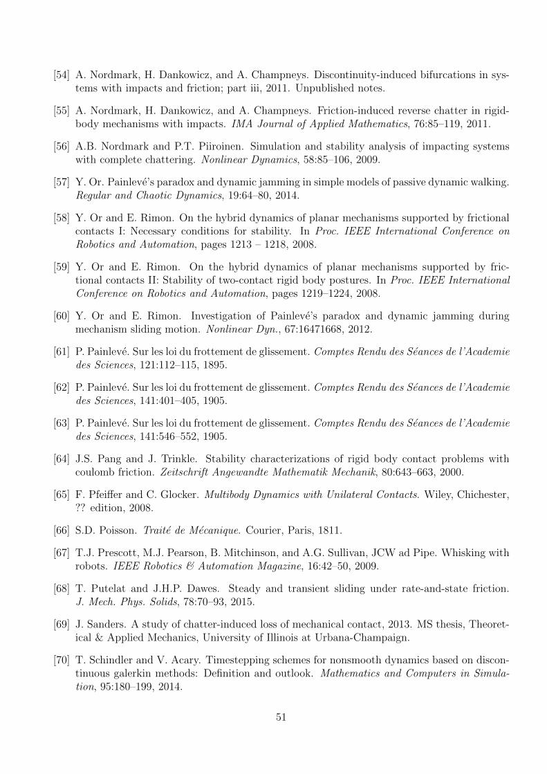
[54] A. Nordmark, H. Dankowicz, and A. Champneys. Discontinuity-induced bifurcations in sys-tems with impacts and friction; part iii, 2011. Unpublished notes.

[55] A. Nordmark, H. Dankowicz, and A. Champneys. Friction-induced reverse chatter in rigid-body mechanisms with impacts. IMA Journal of Applied Mathematics, 76:85–119, 2011.

[56] A.B. Nordmark and P.T. Piiroinen. Simulation and stability analysis of impacting systemswith complete chattering. Nonlinear Dynamics, 58:85–106, 2009.

[57] Y. Or. Painleve’s paradox and dynamic jamming in simple models of passive dynamic walking.Regular and Chaotic Dynamics, 19:64–80, 2014.

[58] Y. Or and E. Rimon. On the hybrid dynamics of planar mechanisms supported by frictionalcontacts I: Necessary conditions for stability. In Proc. IEEE International Conference onRobotics and Automation, pages 1213 – 1218, 2008.

[59] Y. Or and E. Rimon. On the hybrid dynamics of planar mechanisms supported by fric-tional contacts II: Stability of two-contact rigid body postures. In Proc. IEEE InternationalConference on Robotics and Automation, pages 1219–1224, 2008.

[60] Y. Or and E. Rimon. Investigation of Painleve’s paradox and dynamic jamming duringmechanism sliding motion. Nonlinear Dyn., 67:16471668, 2012.

[61] P. Painleve. Sur les loi du frottement de glissement. Comptes Rendu des Seances de l’Academiedes Sciences, 121:112–115, 1895.

[62] P. Painleve. Sur les loi du frottement de glissement. Comptes Rendu des Seances de l’Academiedes Sciences, 141:401–405, 1905.

[63] P. Painleve. Sur les loi du frottement de glissement. Comptes Rendu des Seances de l’Academiedes Sciences, 141:546–552, 1905.

[64] J.S. Pang and J. Trinkle. Stability characterizations of rigid body contact problems withcoulomb friction. Zeitschrift Angewandte Mathematik Mechanik, 80:643–663, 2000.

[65] F. Pfeiffer and C. Glocker. Multibody Dynamics with Unilateral Contacts. Wiley, Chichester,?? edition, 2008.

[66] S.D. Poisson. Traite de Mecanique. Courier, Paris, 1811.

[67] T.J. Prescott, M.J. Pearson, B. Mitchinson, and A.G. Sullivan, JCW ad Pipe. Whisking withrobots. IEEE Robotics & Automation Magazine, 16:42–50, 2009.

[68] T. Putelat and J.H.P. Dawes. Steady and transient sliding under rate-and-state friction.J. Mech. Phys. Solids, 78:70–93, 2015.

[69] J. Sanders. A study of chatter-induced loss of mechanical contact, 2013. MS thesis, Theoret-ical & Applied Mechanics, University of Illinois at Urbana-Champaign.

[70] T. Schindler and V. Acary. Timestepping schemes for nonsmooth dynamics based on discon-tinuous galerkin methods: Definition and outlook. Mathematics and Computers in Simula-tion, 95:180–199, 2014.

51

[71] T. Schnidler, B. Nguyen, and J. Trinkle. Understanding the difference between prox and com-plementarity formulations for simulation of systems with contact. In IEEE/RSJ InternationalConference on Intelligent Robotics and Systems, San Francisco, USA, 2011.

[72] Y. Shen. Painleve paradox and dynamic jam of a three-dimensional elastic rod. Archive ofApplied Mechanics, 85:805–816, 2015.

[73] Y.N.A. Shen and W.J. Stronge. Painleve paradox during oblique impact with friction. Eur.J. Mechanics A – Solids, 30:457–467, 2011.

[74] D.E. Stewart. Existence of solutions to rigid body dynamics and the Painleve paradoxes.Comptes Rendus de l’Acedemie des Science Serie I: Matheamtique, 325:689–693, 1997.

[75] D.E. Stewart. Convergence of a time-stepping scheme for rigid-body dynamics and resolutionof Painleve’s problem. Archive for Rational Mechanics and Analysis, 145:215–260, 1998.

[76] D.E. Stewart. Rigid-body dynamics with friction and impact. SIAM Review, 42:339, 2000.

[77] W.J. Strong. Smooth dynamics of oblique impact with friction. International Journal ofImpact Engineering, 51:36–49, 2013.

[78] W.J. Stronge. Rigid body collisions with friction. Proceedings of the Royal Society of London,431:169–181, 1990.

[79] W.J. Stronge. Impact Mechanics. Cambridge University Press, Cambridge, UK, 2000.

[80] W.J. Stronge. Energetically consistent calculations for oblique impact in unbalanced systemswith friction. J. Applied Mechanics – Trans. ASME, 82:art. no. 081003, 2015.

[81] R. Szalai. Impact mechanics of elastic structures with point contact. Journal of Vibrationand Acoustics — Transactions of the ASME, 136:Art. No. 041002, 2014.

[82] R. Szalai. Modelling elastic structures with strong nonlinearities with application to stick-slipfriction. Proc. Roy Soc. Lond. A, 470:Art. No. 20130593, 2014.

[83] P.L. Varkonyi. Dynamics of rigid bodies with multiple frictional contacts: extended analysis,2015. unpublished notes.

[84] P.L. Varkonyi. Dynamics of rigid bodies with multiple frictional contacts: new faces ofpainlevs paradox. In Proc. 13th International Conf. of Dynamical Systems: theory and ap-plications (DSTA), 2015.

[85] P.L. Varkonyi. On the stability of rigid multibody systems with applications to roboticgrasping and locomotion. ASME Journal of Mechanisms and Robotics, 7:041012, 2015.

[86] P.L. Varkonyi, D. Gontier, and J. W. Burdick. On the lyapunov stability of quasistatic planarbiped robots. In IEEE International Conference on Robotics and Automation (ICRA), pages63–70, 2012.

[87] P.L. Varkonyi and Y. Or. Lyapunov stability of a rigid body with two frictional contacts,2015. unpublished notes.

52

[88] A. Wagner, E. Heffel, A.F. Arrieta, G. Spelsberg-Korspeter, and P. Hagedorn. Analysis of anoscillatory Painleve-Klein apparatus with a nonholonomic constraint. Differential Equationsand Dynamical Systems, 21:149–157, 2013.

[89] A.N. Whitehead and B. Russell. Principia Mathematica. Cambridge University Press, Cam-bridge, UK, second edition, 1927.

[90] E.V. Wilms and H. Cohen. The occurrence of Painleves paradox in the motion of a rotatingshaft. J. Appl. Mech., 64:1008–1010, 1997.

[91] J. Woodhouse, T. Putelat, and A. McKay. Are there reliable constitutive laws for dynamicfriction?, 2015. to appear in Phil. Trans. Roy. Soc. Lond A.

[92] Z. Zhao, C. Liu, and B. Chen. The Painleve paradox studied at a 3d slender rod. J. AppliedMechanics – Trans. ASME, 75:art. no. 041006, 2008.

[93] Z. Zhao, C. Liu, B. Chen, and B. Brogliato. Asymptotic analysis of Painleves paradox.Multibody System Dynamics, Published online:DOI: 10.1007/s11044–014–9448–1, 2015.

[94] Z. Zhao, C.S. Liu, W. Ma, and B. Chen. Experimental investigation of the Painleve paradoxin a robotic system. J. Applied Mechanics – Trans. ASME, 75:art. no. 041006, 2008.

[95] A. Zilli, R.J. Williams, and David J. Ewins. Nonlinear dynamics of a simplified model ofan overhung rotor subjected to intermittent annular rubs. J. Eng. Gas Turbines Power –Transactions ASME, 137:Art. No. 065001, 2015.

53