the origin and evolution of saturn’s 2011–2012...

Icarus 221 (2012) 560–586

Contents lists available at SciVerse ScienceDirect

Icarus

journal homepage: www.elsevier .com/ locate/ icarus

The origin and evolution of Saturn’s 2011–2012 stratospheric vortex

Leigh N. Fletcher a,⇑, B.E. Hesman b, R.K. Achterberg b, P.G.J. Irwin a, G. Bjoraker c, N. Gorius d,J. Hurley a, J. Sinclair a, G.S. Orton e, J. Legarreta f, E. García-Melendo g,h, A. Sánchez-Lavega i,P.L. Read a, A.A. Simon-Miller c, F.M. Flasar c

a Atmospheric, Oceanic & Planetary Physics, Department of Physics, University of Oxford, Clarendon Laboratory, Parks Road, Oxford OX1 3PU, UKb Department of Astronomy, University of Maryland, College Park, MD 20742, USAc NASA/Goddard Spaceflight Center, Greenbelt, MD 20771, USAd Department of Physics, The Catholic University of America, Washington, DC 20064, USAe Jet Propulsion Laboratory, California Institute of Technology, 4800 Oak Grove Drive, Pasadena, CA 91109, USAf Departamento de Ingeniera de Sistemas y Automtica, EUITI, Universidad del Pas Vasco UPV/EHU, Bilbao, Spaing Esteve Duran Observatory Foundation. Avda. Montseny 46, Seva 08553, Spainh Institut de Cincies de lEspai (CSIC-IEEC), Campus UAB, Facultat de Cincies, Torre C5, parell, 2a pl., Bellaterra E-08193, Spaini Departamento de Fsica Aplicada I, E.T.S. Ingenieros, Universidad del Pas Vasco, Alameda Urquijo s/n, Bilbao 48013, Spain

a r t i c l e i n f o

Article history:Received 29 June 2012Revised 13 August 2012Accepted 14 August 2012Available online 1 September 2012

Keywords:SaturnAtmospheres, CompositionAtmospheres, Structure

0019-1035/$ - see front matter � 2012 Elsevier Inc. Ahttp://dx.doi.org/10.1016/j.icarus.2012.08.024

⇑ Corresponding author.E-mail address: [email protected] (L.N. Fletch

a b s t r a c t

The planet-encircling springtime storm in Saturn’s troposphere (December 2010–July 2011, Fletcher, L.N.et al. [2011]. Science 332, 1413–1414; Sánchez-Lavega, A. et al. [2011]. Nature 475, 71–74; Fischer, G. etal. [2011]. Nature 475, 75–77) produced dramatic perturbations to stratospheric temperatures, winds andcomposition at mbar pressures that persisted long after the tropospheric disturbance had abated. Ther-mal infrared (IR) spectroscopy from the Cassini Composite Infrared Spectrometer (CIRS), supported byground-based IR imaging from the VISIR instrument on the Very Large Telescope and the MIRSI instru-ment on NASA’s IRTF, is used to track the evolution of a large, hot stratospheric anticyclone between Jan-uary 2011 and March 2012. The evolutionary sequence can be divided into three phases: (I) the formationand intensification of two distinct warm airmasses near 0.5 mbar between 25 and 35�N (B1 and B2)between January–April 2011, moving westward with different zonal velocities, B1 residing directly abovethe convective tropospheric storm head; (II) the merging of the warm airmasses to form the large single‘stratospheric beacon’ near 40�N (B0) between April and June 2011, disassociated from the storm headand at a higher pressure (2 mbar) than the original beacons, a downward shift of 1.4 scale heights(approximately 85 km) post-merger; and (III) the mature phase characterised by slow cooling(0.11 ± 0.01 K/day) and longitudinal shrinkage of the anticyclone since July 2011. Peak temperatures of221.6 ± 1.4 K at 2 mbar were measured on May 5th 2011 immediately after the merger, some 80 K war-mer than the quiescent surroundings. From July 2011 to the time of writing, B0 remained as a long-livedstable stratospheric phenomenon at 2 mbar, moving west with a near-constant velocity of2.70 ± 0.04 deg/day (�24.5 ± 0.4 m/s at 40�N relative to System III longitudes). No perturbations to visibleclouds and hazes were detected during this period.

With no direct tracers of motion in the stratosphere, we use thermal windshear calculations to estimateclockwise peripheral velocities of 200–400 m/s at 2 mbar around B0. The peripheral velocities of the twooriginal airmasses were smaller (70–140 m/s). In August 2011, the size of the vortex as defined by theperipheral collar was 65� longitude (50,000 km in diameter) and 25� latitude. Stratospheric acetylene(C2H2) was uniformly enhanced by a factor of three within the vortex, whereas ethane (C2H6) remainedunaffected. The passage of B0 generated a new band of warm stratospheric emission at 0.5 mbar at itsnorthern edge, and there are hints of warm stratospheric structures associated with the beacons at higheraltitudes (p < 0.1 mbar) than can be reliably observed by CIRS nadir spectroscopy. Analysis of the zonalwindshear suggests that Rossby wave perturbations from the convective storm could have propagatedvertically into the stratosphere at this point in Saturn’s seasonal cycle, one possible source of energyfor the formation of these stratospheric anticyclones.

� 2012 Elsevier Inc. All rights reserved.

ll rights reserved.

er).

http://dx.doi.org/10.1016/j.icarus.2012.08.024

mailto:[email protected]

http://dx.doi.org/10.1016/j.icarus.2012.08.024

http://www.sciencedirect.com/science/journal/00191035

http://www.elsevier.com/locate/icarus

L.N. Fletcher et al. / Icarus 221 (2012) 560–586 561

1. Introduction

The outbreak and evolution of a spectacular springtime storm inSaturn’s northern mid-latitudes in 2010–2011 (Fletcher et al.,2011; Sánchez-Lavega et al., 2011; Fischer et al., 2011) capturedthe imaginations of amateurs and professionals alike, spurring aninternational observing campaign to support the orbital high-reso-lution observations from the Cassini spacecraft. Infrared observa-tions by the Cassini Composite Infrared Spectrometer (CIRS,Flasar et al., 2004) and the Very Large Telescope (VLT) determinedthe thermal structure of a saturnian storm for the first time, reveal-ing that the convective storm cells seen in visible imaging pro-duced unexpectedly large perturbations to stratospherictemperatures near 20–40�N (all latitudes in this article are givenas planetographic, and all longitudes as System III west Seidelmannet al., 2007), hundreds of kilometres above the roiling cloud decksof the troposphere. Those stratospheric anomalies, referred to as‘beacons’ of emission, were expected to cool as the storm abated,but instead their evolution through 2011 and 2012 have revealedan entirely new phenomenon in a giant planet stratosphere: theformation and evolution of a giant stratospheric vortex. This articletraces the temperatures, winds and composition of Saturn’s strato-sphere as the vortex evolved in 2011 and 2012.

Historical records in reflected sunlight over the past 130 yearsshow that Saturn’s planetary-scale disturbances exhibit an epi-sodic behaviour and usually occur after summer solstice (Sán-chez-Lavega et al., 1991), with kronocentric solar longitudes (i.e.,Saturn-centric, Ls) in the range from 110� to 167�, measured fromthe spring equinox at Ls = 0� (August 15th, 2009). However, thiscurrent storm started on December 5th 2010 (Ls = 16�), the activeconvection stage persisted until around July 2011 (Ls = 23�), andthe stratospheric beacon remains present at the time of writing(Ls = 32�). This is 9 Earth-years (more that a saturnian season) ear-lier than would be expected from the normal summertime stormoccurrence, making this our first example of a planetary-scalespringtime storm. There is evidence that spring is an importanttime, dynamically, on other planets too, as revealed by enhancedcloud activity during Uranus’ 2007 equinox (e.g., Sromovskyet al., 2009), although the mechanisms driving this seasonal activ-ity are poorly understood.

The cloud-top evolution of the tropospheric disturbance hasbeen well-documented in reflected sunlight from both the Cassinispacecraft (Sayanagi et al., 2012) and ground-based observers(Sánchez-Lavega et al., 2012), and shows similarities with previous‘Great White Storm’ events on Saturn (Sánchez-Lavega, 1982; Sán-chez-Lavega et al., 1991). The first visible observations of the stormcoincided with the detection of abundant electrical activity by theRadio and Plasma Wave Science instrument onboard Cassini(Fischer et al., 2011). The powerful upwelling of moist air in multi-ple storm cells in the convecting area was accompanied by near-continuous lightning discharges driven by Saturn’s internal heat(peaking at ten Saturn electrostatic discharges, or SEDs, per second,Fischer et al., 2011). However, the unprecedented resources pro-vided by the infrared instrumentation on Cassini and the high spa-tial resolution afforded by the 8-m class of ground-basedobservatories provided our first observations of the thermal struc-ture of a saturnian storm (Fletcher et al., 2011).

Thermal imaging of the storm showed that a cold, compact(4000 � 5500 km, ±800 km) anticyclonic vortex had formed in theupper troposphere near 41�N planetographic latitude to the eastof the storm head within the first few days of the storm onset. Thislarge, cold tropospheric oval in Fig. 1 of Fletcher et al. (2011)appeared a dark bluish colour in visible imaging and was sur-rounded by a collar of whiter clouds. The oval propagated westwardwith the retrograde jet at 39�N, albeit slower than the velocity of

the storm head (Sánchez-Lavega et al., 2011). The tropospheric vor-tex marked a distinct boundary between the storm head to the westand the easterly tail, rather like Jupiter’s Great Red Spot perturbingjet streams around its periphery to create the turbulent wake ofJupiter’s South Equatorial Belt (SEB).

VLT and Cassini imaging, sensitive to stratospheric emissionfrom methane and ethane (7.9, 8.6 and 12.3 lm), demonstratedsubstantial perturbations to the stably-stratified upper atmo-sphere to pressures as low as 0.5 mbar (Fletcher et al., 2011). Thecompact tropospheric vortex was flanked at high altitude to theeast and west by the diffuse warm airmasses known as strato-spheric beacons. In this paper we extend the observations to trackthe surprising evolution of the beacons after their initial discovery.In Section 2 we discuss the Cassini and ground-based instrumentsused to track Saturn’s stratospheric emission from January 2011 toMarch 2012, plus our analysis and modelling techniques. The evo-lution of the beacons is described in Section 3, before we determinethe atmospheric temperatures, winds, stability and hydrocarboncomposition associated with the beacons in Section 4. We discussmechanisms and numerical simulations for the origins of thestratospheric beacons in Section 5 before highlighting the key con-clusions of this infrared study in Section 6.

2. Sources of data

The evolution of Saturn’s stratospheric thermal-infrared (IR)emission was monitored throughout 2011 and 2012 using threedifferent resources: spectroscopic mapping from the CompositeInfrared Spectrometer (CIRS, Flasar et al., 2004) on the Cassini or-biter (observation details in Table 1); high spatial resolution imag-ing in the N band (8–14 lm) from the ESO (European SouthernObservatory) Very Large Telescope (VLT) mid-IR camera/spectrom-eter (VISIR, Lagage et al. (2004) observation details in Table 2); andmoderate spatial resolution N-band imaging from NASA’s InfraredTelescope Facility (IRTF) mid-IR spectrometer and imager (MIRSI,Deutsch et al., 2003 observation details in Table 3). We describethe data acquisition and reduction in the following sections, beforediscussing the observations in Section 3.

2.1. Cassini/CIRS spectroscopy

Cassini/CIRS (see Flasar et al. (2004) for a complete description)comprises two interferometers fed by a shared telescope and fore-optics. The polarising Martin–Puplett far-IR interferometer (10–600 cm�1, known as focal plane 1, or FP1) will not be used in thepresent stratospheric analysis, as its sensitivity is primarily tropo-spheric. Instead, we use the mid-IR Michelson interferometer,which features two arrays of 1 � 10 HdCdTe detectors (focal planes3 and 4, or FP3, 600–1100 cm�1 and FP4, 1100–1500 cm�1) with aninstantaneous field of view (IFOV) of 0.27 � 0.27 mrad. Observa-tions use pairs of pixels coadded as a single 0.27 � 0.54 mrad pixel.CIRS has a programmable spectral resolution from 0.5 to15.5 cm�1, with the highest spectral resolutions used for composi-tional studies and the lowest resolution used for mapping temper-ature perturbations.

Four different observational templates were used to study thebeacon evolution (Table 1). The storm was mapped at the highestspatial resolution of 0.4� latitude (equivalent to 310 km at 40�N)on August 21st 2011 and January 27th 2012 using the 15.5 cm�1

spectral resolution setting used for mapping (known as a FIRMAP),where the fields of view are repeatedly scanned along the centralmeridian as Saturn’s 10-h rotation sweeps out a longitude circle.The majority of observations used a ‘sit-and-stare’ technique at aparticular latitude at 0.5 or 2.5 cm�1 spectral resolution (known

Table 1Cassini/CIRS observations of the storm location. Some dates are grouped together to form better spatial maps in Fig. 3.

Start time (UTC) Stop time (UTC) Identifier Resolution Comments

05-October-2010 15:15 06-October-2010 16:14 139_001C 0.5 Pre-storm observation, 20–30�N, maximum 1.7 K contrasts18-October-2010 22:00 19-October-2010 09:59 139_002F 15.0 Southern hemisphere map for VISIR calibration

22-October-2010 06:00 23-October-2010 10:29 139_001MT 2.5 Pre-storm observation

02-January-2011 12:00 02-January-2011 23:59 143_001C 0.5 50�N, published in Fletcher et al. (2011)03-January-2011 00:00 03-January-2011 22:59 143_001M 2.5 65�N

19-January-2011 18:30 20-January-2011 17:29 143_001MT 2.5 Published in Fletcher et al. (2011)

25-February-2011 13:27 25-February-2011 19:26 145_003C 0.5 10�N, captures B1 only as high as 15�N26-February-2011 00:27 26-February-2011 02:26 145_004C 0.5 10�N, no beacon26-February-2011 07:27 26-February-2011 13:26 145_005C 0.5 10�N, captures B2

03-March-2011 15:32 04-March-2011 13:32 145_007C 0.5 25–35�N

06-March-2011 03:32 06-March-2011 09:26 145_008C 0.5 20�N, southern edge of B106-March-2011 14:27 07-March-2011 01:25 146_001I 2.5 ISS Rider for context

09-March-2011 20:13 10-March-2011 02:12 146_001C 0.5 Does not observe beacon10-March-2011 12:29 10-March-2011 18:12 146_002C 0.5 South-eastern side of B1

12-March-2011 06:58 12-March-2011 17:57 146_001M 2.5 55�N Northern side of B112-March-2011 17:58 12-March-2011 23:57 146_003C 0.5 30–40�N, B213-March-2011 18:13 14-March-2011 00:12 146_004C 0.5 30–40�N, B1

14-March-2011 05:14 14-March-2011 11:12 146_005C 0.5 30–40�N, B115-March-2011 13:13 16-March-2011 11:12 146_003M 2.5 45�N, Both beacons but only the northern edge of B2

18-March-2011 04:58 18-March-2011 15:56 146_006C 0.5 Northern edge of B1

25-April-2011 21:30 26-April-2011 20:29 147_001MT 2.5 First merger observation

04-May-2011 16:00 05-May-2011 14:59 148_001M 2.5 30–50�N, Good image of B0

06-July-2011 00:00 06-July-2011 22:59 150_001MT 2.5 Clearly shows the tail at 55�N, Southern edge of B007-July-2011 22:00 08-July-2011 09:59 150_001C 0.5 35–45�N, Centre of B0

26-July-2011 05:00 27-July-2011 03:59 151_001M 2.5 25–45�N, southern portion of B0

30-July-2011 03:47 30-July-2011 20:16 151_001MT 2.5 Northern edge of B001-August-2011 21:38 02-August-2011 15:37 151_001V 2.5 VIMS Rider, northern portion of B0

16-August-2011 03:55 16-August-2011 14:54 152_001M 2.5 15–25�N, southern edge of B0

21-August-2011 18:59 22-August-2011 08:23 152_001F 15.0 Full northern hemisphere map, well-defined tail at 55�N

10-September-2011 07:30 10-September-2011 19:29 153_001C 0.5 30–40�N, centre of B0

22-October-2011 18:00 23-October-2011 02:54 155_001MT 2.5 Caught the centre of B0

03-December-2011 14:31 04-December-2011 01:38 158_001M 2.5 B0 30–50�N

13-January-2012 11:49 13-January-2012 22:27 159_004C 0.5 B0 35–45�N

19-January-2012 06:20 19-January-2012 12:18 160_004C 0.5 Missed B0 at 40�N19-January-2012 22:20 20-January-2012 04:18 160_005C 0.5 B0 at 40�N

23-January-2012 01:05 23-January-2012 23:04 160_001M 2.5 Southern edge of B0, 10–30�N

27-January-2012 00:31 27-January-2012 11:30 160_001F 15.0 Full northern map

16-February-2012 09:53 16-February-2012 21:52 161_001C 0.5 B0 at 30–40�N

11-March-2012 10:00 11-March-2012 21:59 162_001C 0.5 Northern edge of B0 at 45�N

14-March-2012 20:16 15-March-2012 19:15 162_001M 2.5 B0 at 35–55�N

Table 2VLT/VISIR observations of the storm location. UTC times show the time spent observing Saturn, excluding calibration.

Start time (UTC) Stop time (UTC) Program ID Comments

2011-01-19 07:36 2011-01-19 08:30 386.C-0096(A) First beacon detection, no evidence for tropospheric heating in Q-band filters. B1 near to planetary limb2011-01-27 07:23 2011-01-27 08:15 386.C-0096(A) High humidity, poorer seeing than January 19th, B2 only2011-01-31 07:59 2011-01-31 09:09 386.C-0096(A) Excellent seeing, eight filters, B2 near limb, B1 centred2011-02-08 07:21 2011-02-08 08:21 386.C-0096(A) High humidity, little structure visible, B2 only2011-03-25 02:57 2011-03-25 09:38 386.C-0096(B) Observed both hemispheres, excellent structure in B1, B22011-03-26 03:16 2011-03-26 06:59 386.C-0096(B) B2 only, repeat of previous night, still no detection in Q-band filters2011-05-25 22:40 2011-05-25 23:33 386.C-0096(A) Post-merger, B0 now visible in all filters, including Q-band2011-06-26 23:01 2011-06-27 00:09 287.C-5032(A) B0 near central meridian2011-07-20 23:04 2011-07-20 23:59 287.C-5032(A) B0 on central meridian2011-07-24 23:24 2011-07-25 00:14 287.C-5032(A) Final B0 observation from VLT, beacon evident in Q and N-band filters

562 L.N. Fletcher et al. / Icarus 221 (2012) 560–586

as COMPSITs and MIRMAPs, respectively), aligning the arraysnorth–south and allowing Saturn’s rotation to sweep the arraysacross all longitudes. These observations were taken at a greaterdistance from Saturn, yielding spatial resolutions of 1–2� longitude

(800–1600 km at 40�N) and 2–4� latitude in swaths 10–20� lati-tude wide. Those observations that captured part of the strato-spheric disturbance are recorded in Table 1. Finally, MIRTMAPsuse the 2.5 cm�1 spectral resolution setting, but in this case the

Table 3IRTF/MIRSI observations of the storm location. UTC times show the time spent observing Saturn, excluding calibration.

Date Start time (UTC) Stop time (UTC) Program ID Comments

2011-03-25 12:47 14:22 011 Captured B2 (near centre)2011-03-26 13:53 15:42 011 B1 on the rising limb2011-04-26 05:56 09:17 006 Tail of B1 emission, rising on western limb2011-04-27 05:14 09:05 006 B1 rising on the limb2011-04-28 07:42 09:19 (Engineering time) B1 on central meridian2011-05-22 08:39 09:40 (Engineering time) Post-merger, B0 towards setting limb2011-05-23 08:27 10:44 (Engineering time) Beacon tail region2011-07-24 02:21 03:18 010 B0 near centre disc in poor seeing2011-07-27 02:17 03:28 010 B0 on rising limb, poor seeing2011-08-02 02:22 04:20 (Engineering time) Tail region of B02011-08-03 02:03 04:20 (Engineering time) B0 on setting limb2011-08-04 02:42 04:34 (Engineering time) B0 rising to central meridian2011-08-05 02:18 04:19 (Engineering time) B0 from centre to setting limb2011-08-31 01:05 03:06 027 B0 on setting limb2011-09-01 00:05 03:56 027 Tail region of B0, final MIRSI observation


focal planes are stepped from north to south (‘shift and stare’),dwelling on a particular latitude for approximately 1.5 h (50� oflongitude). All spectra were extracted from the most recent Cas-sini/CIRS calibrated database (version 3.2, which uses deep spaceinterferograms within ±8 h of the target interferograms for radio-metric calibration), and were coadded to improve the signal tonoise as necessary in Section 4. As the number of target interfero-grams in each observation exceeds the number of cold deep spacecalibration spectra, we find that the noise equivalent spectral radi-ances (NESR), and hence the retrieval uncertainty for each bin, isdominated by the measurement uncertainties on the deep spacespectra.

2.2. VLT/VISIR imaging

The spectroscopic observations from Saturn orbit were supple-mented by ground-based VLT thermal-IR filtered imaging to pro-vide contextual information for the stratospheric disturbancebetween January and July 2011 when the planet was visible (Table2). VISIR observations (Lagage et al., 2004) were obtained in twoprograms using the Melipal (UT3) telescope at Cerro Paranal inChile: a regular program 386.C-0096 (January–May 2011) andDirector’s Discretionary program 287.C-5032 (June–July 2011).The goal for each run was to obtain images of Saturn at eight dis-crete wavelengths – 17.6, 18.7 and 19.5 lm to constrain tropo-spheric temperatures from the H2–He collisionally-inducedcontinuum; 9.0 and 10.7 lm for tropospheric PH3; and 7.9, 8.6and 12.3 lm for stratospheric temperatures via emission fromCH4, CH3D and C2H6, respectively. It is these latter three filters thathave been used in this study.

Quantitative comparison of filtered images is challenging – see-ing conditions and the water vapour humidity varied between eachrun, and the range to Saturn varied between 8.6 and 9.9 AU duringthe 2011 campaign. This meant that the diffraction-limited spatialresolution using the 8.1-m diameter primary mirror varied be-tween 1530 and 1760 km for 7.9 lm (0.2500), and 2380–2740 kmfor 12.3 lm (0.3800) on Saturn’s disc. In practice, the seeing coulddegrade to 1.000 during an observation, equivalent to 6240–7180 km on Saturn’s disc, depending on the Earth to Saturn dis-tance. However, these ground-based images proved vital in tracingthe motion and size of the beacons in Section 3.

Two or more images were obtained in each filter, dithered onthe array to allow removal of bad pixels. Images on each date wereselected based on their display of the beacon, and are shown inFig. 1. The ESO data pipeline was used for initial reduction andbad-pixel removal via its front-end interface, Gasgano (version2.3.0). Images were geometrically registered and cylindricallyreprojected using the techniques described in Fletcher et al.

(2009c). Images in each filter were radiometrically calibrated byscaling the flux to match a Cassini/CIRS FIRMAP (15.5 cm�1) obser-vation of the southern hemisphere on October 18th 2010 (i.e.,avoiding the northern perturbations). The CIRS data were con-volved with the VISIR filter functions prior to the scaling.

2.3. IRTF/MIRSI imaging

In addition to VLT/VISIR observations, we undertook a campaignof MIRSI (Deutsch et al., 2003) mid-IR imaging using the 3-m pri-mary mirror of the IRTF (Table 3). These were subdivided into sixdiscrete observing runs between March and September 2011, andeach observing run featured imaging in a number of discrete filters,similar to those given for VLT/VISIR. Only the 7.9 and 12.3-lm fil-ters are considered in this study. During the course of the 2011observations, Saturn varied from 8.6 to 10.4 AU from Earth, imply-ing that the diffraction-limited spatial resolution varied from 4130to 5000 km at 7.9 lm (0.6600) and 6430–7780 km at 12.3 lm (1.000).The data acquisition and reduction procedures are described inFletcher et al. (2009c): chopping and nodding were used to elimi-nate the background sky emission and thermal interference; skysubtraction and flat-fielding were applied to remove variations inthe background across the detector; and five images (ditheredaround the array to eliminate corrupted pixels) were coadded toproduce the final MIRSI images. These MIRSI images were usedto monitor the evolution of the beacons in Section 3.

2.4. Spectral modelling

Inspection of the raw data can tell us a great deal (e.g., mappingthe spatial extent and position of the stratospheric airmasses in Sec-tion 3), but a better understanding of the atmospheric effects of the2010 storm can be gained by modelling the CIRS spectra. We employa radiative transfer and optimal estimation retrieval code (Nemesis,Irwin et al., 2008) to determine the vertical temperature structurefrom the CH4 and H2 emissions, and the molecular abundances ofhydrocarbons from their emission features. The retrieval modelhas been fully described elsewhere (Irwin et al., 2008; Fletcheret al., 2010), but we review the important details here.

Saturn’s reference atmospheric structure was defined on 120pressure levels equally spaced in log(p) between 1 lbar and10 bar. An a priori temperature profile was estimated as a meanof Cassini/CIRS T(p) profiles between ±45� latitude from Cassini’sprime mission using nadir data from Fletcher et al. (2010) (sensi-tive to 1–800 mbar) and limb results from Guerlet et al. (2009)(sensitive to 1 lbar to 20 mbar). The helium abundance He/H2

was set to 0.135 (Conrath and Gautier, 2000). The PH3 profilewas initially set to the CIRS-derived mole fraction of 6.4 ppm at

Fig. 1. VLT/VISIR imaging of Saturn’s stratospheric emission from January to July 2011. A white outline in the upper and lower panels shows the planetary limb, andobservation times and central meridian longitudes are given for each image. The scale runs linearly from minimum to maximum radiance for each figure. B1 and B2 arelabelled, and the rings can be seen as a dark, absorbing arc south of the equator. The eight images in the upper panel show CH3D emission at 8.6 lm (sensitive to the 1.0–5.7 mbar region, peaking at 2.5 mbar); the central panel shows C2H2 emission at 13.0 lm (0.9–7.1 mbar, peaking at 2.6 mbar); and the bottom eight images show C2H6

emission at 12.3 lm (sensitive to the 0.9–9.0 mbar region, peaking at 3.3 mbar). The contribution functions for each filter were calculated for the warm temperatures of thebeacon. Observations on March 25th captured both B1 (lower left, with arrows indicating three satellite spots ‘SS’) and B2 (upper right) on the same night, whereasobservations in July caught B0 at the centre of the disc. The contrast between the beacon and the rest of the disc is greatest at 8.6 lm.


p > 0.55 bar, decreasing due to photolysis at lower pressures with afractional scale height of 0.27 (the ratio of the PH3 scale height tothe scale height of the bulk atmosphere, Fletcher et al., 2009a).The vertical distribution of NH3 had a reference mole fraction of100 ppm below 1 bar, decreasing with altitude following a satu-rated vapour pressure profile (p > 0.3 bar) and a linear extrapola-tion to low pressures to represent photolysis (p < 0.3 bar). TheCH4 mole fraction was set to a deep value of 4.7 � 10�3 (Fletcheret al., 2009b) and drops with altitude due to both diffusive pro-cesses and photochemical destruction towards the homopause,

as reviewed by Moses et al. (2000). Our a priori hydrocarbon pro-files were taken as the low-latitude mean (between ±30� latitude)of profiles published by Guerlet et al. (2009) using CIRS limb spec-troscopy, which were themselves based on photochemical model-ling from Moses and Greathouse (2005). This reference atmosphereis available from the principal author on request.

The sources of spectroscopic linedata for these gases are pre-sented in Table 4. These data were used to generate k-distributions(ranking absorption coefficients, k, according to their frequencydistribution, Irwin et al., 2008) using evenly-sampled wavenumber

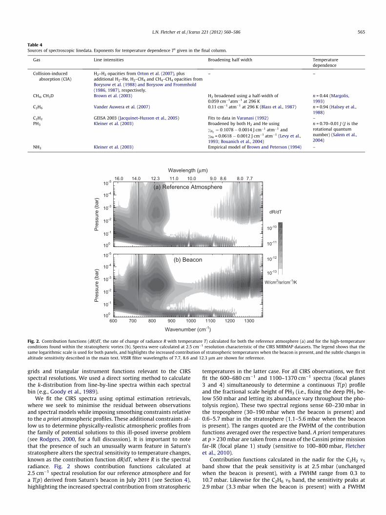
Table 4Sources of spectroscopic linedata. Exponents for temperature dependence Tn given in the final column.

Gas Line intensities Broadening half width Temperaturedependence

Collision-inducedabsorption (CIA)

H2–H2 opacities from Orton et al. (2007), plusadditional H2–He, H2–CH4 and CH4–CH4 opacities fromBorysow et al. (1988) and Borysow and Frommhold(1986, 1987), respectively.

– –

CH4, CH3D Brown et al. (2003) H2 broadened using a half-width of0.059 cm�1atm�1 at 296 K

n = 0.44 (Margolis,1993)

C2H6 Vander Auwera et al. (2007) 0.11 cm�1 atm�1 at 296 K (Blass et al., 1987) n = 0.94 (Halsey et al.,1988)

C2H2 GEISA 2003 (Jacquinet-Husson et al., 2005) Fits to data in Varanasi (1992) –PH3 Kleiner et al. (2003) Broadened by both H2 and He using

cH2¼ 0:1078� 0:0014 J cm�1 atm�1 and

cHe = 0.0618 � 0.0012 J cm�1 atm�1 (Levy et al.,1993; Bouanich et al., 2004)

n = 0.70–0.01 J (J is therotational quantumnumber) (Salem et al.,2004)

NH3 Kleiner et al. (2003) Empirical model of Brown and Peterson (1994) –

100

10-1

10-2

10-3

10-4

10-5

Pres

sure

(bar

)

7.7 8.0 8.6 9.0 10.0 11.0 12.3 14.0 16.0

Wavelength (μm)

600 700 800 900 1000 1100 1200 1300

Wavenumber (cm-1)

100

10-1

10-2

10-3

10-4

10-5

Pres

sure

(bar

)

10-13

10-12

10-11

10-10

dR/dT

W/cm2/sr/cm-1/K

(a) Reference Atmosphere

(b) Beacon

Fig. 2. Contribution functions (dR/dT, the rate of change of radiance R with temperature T) calculated for both the reference atmosphere (a) and for the high-temperatureconditions found within the stratospheric vortex (b). Spectra were calculated at 2.5 cm�1 resolution characteristic of the CIRS MIRMAP datasets. The legend shows that thesame logarithmic scale is used for both panels, and highlights the increased contribution of stratospheric temperatures when the beacon is present, and the subtle changes inaltitude sensitivity described in the main text. VISIR filter wavelengths of 7.7, 8.6 and 12.3 lm are shown for reference.


grids and triangular instrument functions relevant to the CIRSspectral resolutions. We used a direct sorting method to calculatethe k-distribution from line-by-line spectra within each spectralbin (e.g., Goody et al., 1989).

We fit the CIRS spectra using optimal estimation retrievals,where we seek to minimise the residual between observationsand spectral models while imposing smoothing constraints relativeto the a priori atmospheric profiles. These additional constraints al-low us to determine physically-realistic atmospheric profiles fromthe family of potential solutions to this ill-posed inverse problem(see Rodgers, 2000, for a full discussion). It is important to notethat the presence of such an unusually warm feature in Saturn’sstratosphere alters the spectral sensitivity to temperature changes,known as the contribution function dR/dT, where R is the spectralradiance. Fig. 2 shows contribution functions calculated at2.5 cm�1 spectral resolution for our reference atmosphere and fora T(p) derived from Saturn’s beacon in July 2011 (see Section 4),highlighting the increased spectral contribution from stratospheric

temperatures in the latter case. For all CIRS observations, we firstfit the 600–680 cm�1 and 1100–1370 cm�1 spectra (focal planes3 and 4) simultaneously to determine a continuous T(p) profileand the fractional scale height of PH3 (i.e., fixing the deep PH3 be-low 550 mbar and letting its abundance vary throughout the pho-tolysis region). These two spectral regions sense 60–230 mbar inthe troposphere (30–190 mbar when the beacon is present) and0.6–5.7 mbar in the stratosphere (1.1–5.6 mbar when the beaconis present). The ranges quoted are the FWHM of the contributionfunctions averaged over the respective band. A priori temperaturesat p > 230 mbar are taken from a mean of the Cassini prime missionfar-IR (focal plane 1) study (sensitive to 100–800 mbar, Fletcheret al., 2010).

Contribution functions calculated in the nadir for the C2H2 m5

band show that the peak sensitivity is at 2.5 mbar (unchangedwhen the beacon is present), with a FWHM range from 0.3 to10.7 mbar. Likewise for the C2H6 m9 band, the sensitivity peaks at2.9 mbar (3.3 mbar when the beacon is present) with a FWHM


range from 0.4 to 9.4 mbar. These changes in altitude sensitivitydepending on the atmospheric temperature are fully accountedfor in the retrieval process. As the hydrocarbon contribution func-tions extend into the lower stratosphere to altitudes not coveredby the CH4 m4 emission (Fig. 2), we found it necessary to updateour T(p) profiles very slightly while simultaneously scaling thehydrocarbon profiles to fit the 680–860 cm�1 spectrum. The endproduct is a vertical T(p) profile (0.5 < p < 230 mbar) plus estimatesof (i) the ethane and acetylene abundances near 2 mbar; and (ii)the phosphine gradient in the 100 < p < 550 mbar range.

3. Observations: the evolution of the beacon

Although the roiling convective activity in the troposphere hadlargely subsided by July 2011 (Sánchez-Lavega et al., 2012; Sayan-agi et al., 2012), the stratospheric aftermath continued to the timeof writing. The bright stratospheric airmasses dominated Saturn’sappearance at 7.9, 8.6, 12.3 and 13.0 lm (as shown in the VLT/VIS-IR imaging in Fig. 1), and the beacons could only be studied viatheir infrared emission which is mapped with latitude and longi-tude in Fig. 3. These figures consist of both VLT/VISIR 12.3-lmimages (these were of a higher signal to noise than the 7.9-lmimages) and reprojected Cassini/CIRS data averaged between1290 and 1310 cm�1 (the peak of the m4 emission band of CH4),showing the westward motion of the beacons. The longitude ofthe beacons (in System III West) is recorded from Cassini, VLTand IRTF in Fig. 4. The maximum brightness temperature averagedover the 1290–1310 cm�1 spectral range from the CIRS observa-tions is shown in Fig. 5a, showing the variation in the intensityof the beacons. Uncertainties in the emission strength are standarddeviations on the mean estimated within 5� of the beacon centre.

The longitudinal and latitudinal width of the warm airmasses israther subjective, as it depends upon the selected ‘boundary’ of thebeacons (we shall see in Section 4 that more accurate widths canbe estimated from the maximal thermal windshear). In realitythere is a continuous temperature gradient between the beaconcore and the exterior, with no well-defined boundary to define asize. We elected to take the FWHM of the beacon compared tothe quiescent background to demonstrate general trends in themorphology, and we plot the longitudinal width in Fig. 5b andthe latitudinal extent of the beacon in Fig. 5c.

The evolutionary sequence can be divided into three phases:(Phase I) the formation and intensification of two distinct warmairmasses between January and April 2011; (Phase II) the mergingand deceleration to form the large single beacon between April andJune 2011; and (Phase III) the acceleration and slow cooling of thebeacon since July 2011. Each phase is described below, and our re-sults are summarised in Table 5.

3.1. Phase I: formation and intensification

The first Cassini thermal-IR observations of the storm latitudesoccurred on January 2nd 2011, a month after the onset of the dis-turbance (Fig. 3). Previous observations in October 2010 showedlongitudinal homogeneity, with no perturbations to stratospherictemperatures exceeding 2 K. Two warm airmasses were observedin January flanking a central cool region, with longitudinal bright-ness temperature contrasts of 13–15 K at 7.7 lm. Cassini/CIRS cap-tured only the northern edges of the two airmasses at 50–55�N onJanuary 2nd, but later observed the centres of the warm airmasseswith a crude map on January 19th–20th.

The VLT/VISIR 8.6- and 12.3-lm images on January 19th (Fig. 1)confirmed the presence of a central cool stratosphere flanked at theeastern and western edges by warm airmasses. The westernairmass, hereafter beacon one (B1), appeared more diffuse and ex-

tended, sitting above the bulbous white storm head observed invisible imaging. By comparison, the eastern airmass (beacon two,B2) was smaller and more confined. In these early stages, B2 ap-peared to be divided into two distinct warm regions in the VISIRimaging – one was over the ‘northern branch’ of the storm tailand was further to the east; the other existed over the ‘southernbranch’ of the tail – but this split morphology was only observedonce (January 19th 2011). By January 27th, the next VISIR observa-tion in Figs. 1 and 3, the two airmasses comprising B2 had mergedto a single warm airmass. By late January it was clear that the dis-tance between B1 and B2 was increasing, suggesting differentvelocities for the two beacons.

The February 8th VISIR observation caught B2 close to the plan-etary limb, where limb brightening effects prevented us fromextracting a reliable measure of the beacon strength (Fig. 1). How-ever, the next CIRS observations on March 4th (Fig. 3) demon-strated substantial warming of the two airmasses since their firstdiscovery in January. Fig. 5a shows that the maximum brightnesstemperatures of the two beacons increased in an approximatelylinear fashion to reach a peak in May 2011.

The March CIRS and VLT observations also suggest that theslower of the two beacons, B2, was at a more southerly latitudethan the faster and more extended beacon, B1. The March 25thVLT/VISIR observations were designed to be obtained over 6 h sothat both hemispheres of the planet could be viewed (Fig. 1 anda cylindrical map in Fig. 3). They also provided one of our clearestviews of the beacon morphologies: B2 was compact and near-cir-cular, centred at 27.8 ± 2.6�N and extending from 18 to 38�N(Fig. 5c). B1 had a more unusual shape, extending from southwestto northeast and centred near 33.2 ± 2.1�N. B1 had formed its own‘tail’ of warm air, centred on 50�N but extending from 45 to 55�N.The most northerly stratospheric perturbations occurred north ofB1 at around 65–70�N. The beacons appeared to produce no per-turbations to the cold north polar region poleward of 70�N(Fig. 1), which is emerging from the darkness of winter shadowfor the first time in 15 years. The images of B1 on March 25th(Fig. 1) show considerable structure in the extended emissionaround the central warm spot – at least three ‘satellite’ spots canbe seen to the northeast, merging into the extended tail. The fateof these satellites is uncertain, as they were not imaged again be-fore B1 and B2 merged, despite observations of equal spatialresolution.

It is also worth noting that the contrast between the beacon andthe eastern tail is smaller in the 12.3-lm image than in the 8.6-lmin Fig. 1. Calculating contribution functions for each of the VISIR fil-ters under the high-temperature conditions of the beacon, we findthat the 12.3-lm filter senses slightly deeper pressures (0.9–9.0 mbar, peaking at 3.3 mbar) than the 8.6-lm filter (1.0–5.7 mbar, peaking at 2.5 mbar), and that the 8.6-lm filter has anorder of magnitude lower sensitivity to changes in stratospherictemperature than the 12.3-lm filter. Similar differences are ob-served in Fig. 2. Although these differences appear small, theymay suggest a vertical structure to the beacon and tail, to whichwe shall return in Section 4.

3.1.1. Velocities pre-mergerThe Cassini and ground-based observations continued through-

out March and April as the stratospheric emission from the twodiscrete beacons intensified, and B1 completed its traverse of a full360� longitude circle. By this point, enough data were available toquantitatively assess the beacon velocities throughout this period.Extrapolating the motions of the beacons backwards to the time ofthe storm onset in Fig. 4, we find that B1 would have beenat 248�W on December 5th 2010, and B2 at 209�W. The initialtropospheric storm erupted at 242�W Sánchez-Lavega et al.(2011), close to the extrapolated location of B1. We speculate that

2011-01-0320

40

60

Latit

ude

2011-01-2020

40

60

Latit

ude

2011-03-0420

40

60

Latit

ude

2011-03-1120

40

60

Latit

ude

2011-03-1520

40

60

Latit

ude

2011-04-26

20

40

60

Latit

ude

20

40

60

Latit

ude 2011-03-25 (V)

2011-01-27 (V)20

40

60

Latit

ude

2011-05-05

20

40

60

Latit

ude

System III West Longitude360 340 320 300 280 260 240 220 200 180 160 140 120 100 80 60 40 20 0360 340 320 300 280 260 240 220 200 180 160 140 120 100 80 60 40 20 0

System III West Longitude

120130

140

150

160170

2011-07-0620

40

60

Latit

ude

20

40

60

Latit

ude

2011-08-22

2011-07-2620

40

60

Latit

ude

2011-09-1020

40

60

Latit

ude

2011-10-2220

40

60

Latit

ude

2011-12-04

360 340 320 300 280 260 240 220 200 180 160 140 120 100 80 60 40 20 0


20

40

60La

titud

e

2011-06-26 (V)20

40

60

Latit

ude

2011-05-25 (V)20

40

60

Latit

ude

2011-07-20 (V)20

40

60

Latit

ude

2012-01-19

20

40

60

Latit

ude

2012-03-15

360 340 320 300 280 260 240 220 200 180 160 140 120 100 80 60 40 20 0


20

40

60

Latit

ude

2012-02-16

20

40

60

Latit

ude

2012-01-23

20

40

60

Latit

ude

2012-01-13

20

40

60

Latit

ude

120130

140

150

160170

20

40

60

Latit

ude

2012-01-27

Fig. 3. Cylindrically projected maps of Saturn’s CH4 emission between 10� and 70�N from 2011 to 2012. CIRS observations do not provide complete coverage as described inthe main text, but are better-calibrated than the VISIR observations (e.g., third panel from the bottom). Beacon B1 is more extended in the left-hand columns, whereas B2 ismore compact and circular and moves only a small distance before the merger to form B0. The CIRS maps are constructed from the mean brightness temperature between1290 and 1310 cm�1, with the scale bar to the top and bottom of the maps chosen to give the best imaging of the bright beacon and cooler quiescent atmosphere. The VISIRmaps use 12.3-lm images, as these had the highest signal-to-noise of all observations and are morphologically similar to the CIRS maps. Dates refer to the mean time of theobservation, rather than the start time. Small white regions within the CIRS maps indicate ‘missing’ spectra corrupted by calibration defects and flagged by the CIRScalibration pipeline.


these two warm airmasses were generated as a direct result of thedisturbance at 242�W on December 5th 2010, later known as the‘storm head’.

Fig. 4 shows that B1 then moved west at 2.7 ± 0.1 deg/day,equivalent to a velocity of �26.9 ± 1.1 m/s at 33.2�N (the centre ofB1). Co-plotting the longitudes of B1 in the stratosphere and thewhite storm head in the troposphere (Sayanagi et al., 2012), we

see a remarkable co-location of the two features between Januaryand April 2011 (Fig. 4). B1’s velocity is similar to the velocity ofthe storm head (�27.9 ± 0.1 m/s from ground-based observations,Sánchez-Lavega et al., 2012), and consistent with the storm headdrift rate of 2.8 deg/day reported from Cassini/ISS measurements(Sayanagi et al., 2012), suggesting a strong coupling between thetropospheric disturbance and the stratospheric feature. By compar-

0 50 100 150 200 250 300 350 400 450 500

Days since 2011-01-01

-900

90

180

270

360

450

540

630

720

810

900

990

1080

1170

Syst

em II

I Wes

t Lon

gitu

de

01/11 03/11 05/11 07/11 09/11 11/11 01/12 03/12 05/12

DateMotion of Beacons

MIRSI B2MIRSI B1VISIR B2VISIR B1CIRS B2CIRS B1

Phase IIIP IIPhase I

Fig. 4. Tracking the System-III longitude of Saturn’s stratospheric beacons from January 2011 to March 2012 using Cassini/CIRS (black), VLT/VISIR (red) and IRTF/MIRSI (blue).Regression lines (solid) and their errors (dotted) are fitted to data in the three phases described in the main text. The green line shows the longitude of the storm head beforeits disappearance in late June 2011 (Sayanagi et al., 2012). Vertical grey lines show the approximate boundaries between the three phases. The measured velocities are asfollows: for phase I, B1 moves westward by 2.73 ± 0.1 deg/day and B2 by 0.6 ± 0.1 deg/day; B0 moved slowly at 1.6 ± 0.2 deg/day during phase II, and then accelerated to2.70 ± 0.04 deg/day for the remainder of the observing period. (For interpretation of the references to colour in this figure legend, the reader is referred to the web version ofthis article.)


ison, the westward velocity of the small tropospheric anticyclonethat formed east of the storm head was 0.91 deg/day (Sánchez-Lav-ega et al., 2012), which does not seem to correspond to the beaconvelocities in Fig. 4. Plotting the beacon velocities alongside Saturn’stropospheric jet speeds (Sánchez-Lavega et al., 2000) in Fig. 5d, weobserve that both the beacon and the storm head move faster thanthe retrograde jet at 39�N by around 7 m/s, indicating an increase inretrograde velocity from the typical tropospheric cloud decks(around 500 mbar) to the elevated altitudes of the white stormhead (around 200 mbar).

The second beacon, B2, at the more southerly latitude of27.8 ± 2.6�N, also moved to the west but much more slowly(0.6 ± 0.1 deg/day, Fig. 4), equivalent to a westward velocity of�6.2 ± 0.7 m/s at this latitude (Fig. 5d). This difference betweenthe velocities of B1 and B2 caused the two beacons to drift to-gether, intersecting and merging in late April 2011.

3.2. Phase II: merger

Fig. 4 shows that the two beacons occupied the same longitudeon April 30th (day 120, ±3 days). Low spatial-resolution IRTF/MIRSIobservations acquired in late April 2011 showed a single, large hotairmass (hereafter B0), with no distinct boundaries between thetwo independent beacons. The April 26th CIRS MIRTMAP (Fig. 3)shows an extended region of emission, occupying at least 80� longi-tude, with the warmest region at 280�W on that date. The remnantof B1 could still be seen as a secondary peak to the east of the hot-test region, but this had been subsumed into B0 by May 5th, when itwas clear that the interaction between the beacons had formed asingle large hot airmass at 39.5 ± 4.1�N, further north than eitherB1 or B2 and near the centre of the westward jet. The width ofthe warm airmass, as specified by the FWHM (Fig. 5b), spanned

some 90 ± 10� longitude immediately post-merger, and the temper-atures reached their maximum. The maximum brightness temper-ature recorded at 1304 cm�1 was 209.2 K on May 5th 2011 at aspectral resolution of 2.5 cm�1, which is an increase of 70 K com-pared to the typical 140 K brightness temperatures of this latitudecircle (physical temperatures will be discussed in Section 4).

From May 2011 onwards, the beacon was a discrete oval-shaped hot airmass (Fig. 3), wider in east–west extent (approxi-mately 70� wide, equivalent to 55,000 km at 40�N, Fig. 5b) thannorth–south extent (covering approximately 30� in latitude,Fig. 5c). It continued to propagate westward, but more slowly thanbefore, having become detached from the bulbous storm head be-neath. Between April 30th and July 9th 2011 B0 detached from thestorm head and moved west at 1.6 ± 0.2 deg/day (�14.6 ± 1.9 m/sat 39.5 �N), a velocity intermediate between the two original bea-cons B1 and B2.

3.3. Phase III: mature beacon

The final ‘mature’ phase of the beacon B0 is defined to start inlate June or early July 2011 (the exact date is ill-defined due tothe scatter of points in Fig. 4). Visible observations showed thatthe white storm head had encountered the cold anticyclonic vortexin the troposphere between June 15th and 19th 2011 (Sánchez-Lavega et al., 2012). The bulbous white head had dissipated by July12th, and active convection appeared to have ceased, leaving adark tropospheric zone surrounded by disturbed cloud patternsto the north and south. The coupling between this convectionand the beacon velocity is uncertain, but Fig. 4 indicates that B0accelerated in late June or early July to a faster drift velocity of2.70 ± 0.04 deg/day (�24.5 ± 0.4 m/s at 39.5�N). To calculate the

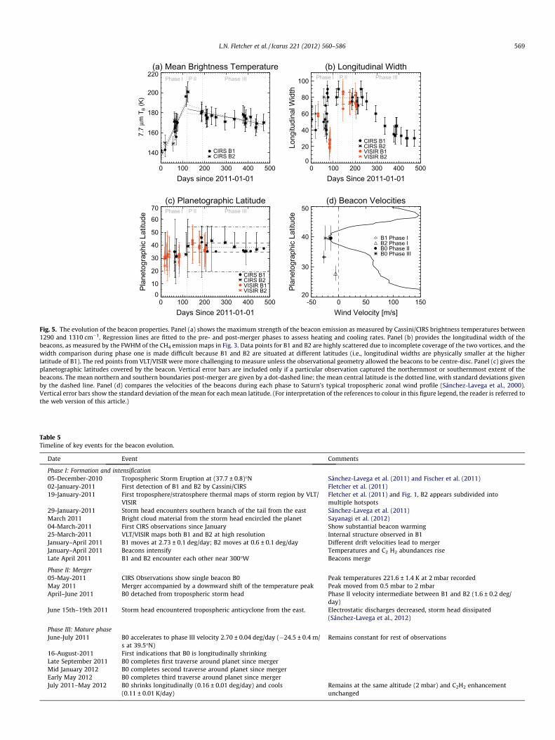
Table 5Timeline of key events for the beacon evolution.

Date Event Comments

Phase I: Formation and intensification05-December-2010 Tropospheric Storm Eruption at (37.7 ± 0.8)�N Sánchez-Lavega et al. (2011) and Fischer et al. (2011)02-January-2011 First detection of B1 and B2 by Cassini/CIRS Fletcher et al. (2011)19-January-2011 First troposphere/stratosphere thermal maps of storm region by VLT/

VISIRFletcher et al. (2011) and Fig. 1, B2 appears subdivided intomultiple hotspots

29-January-2011 Storm head encounters southern branch of the tail from the east Sánchez-Lavega et al. (2011)March 2011 Bright cloud material from the storm head encircled the planet Sayanagi et al. (2012)04-March-2011 First CIRS observations since January Show substantial beacon warming25-March-2011 VLT/VISIR maps both B1 and B2 at high resolution Internal structure observed in B1January–April 2011 B1 moves at 2.73 ± 0.1 deg/day; B2 moves at 0.6 ± 0.1 deg/day Different drift velocities lead to mergerJanuary–April 2011 Beacons intensify Temperatures and C2 H2 abundances riseLate April 2011 B1 and B2 encounter each other near 300�W Beacons merge

Phase II: Merger05-May-2011 CIRS Observations show single beacon B0 Peak temperatures 221.6 ± 1.4 K at 2 mbar recordedMay 2011 Merger accompanied by a downward shift of the temperature peak Peak moved from 0.5 mbar to 2 mbarApril–June 2011 B0 detached from tropospheric storm head Phase II velocity intermediate between B1 and B2 (1.6 ± 0.2 deg/

day)June 15th–19th 2011 Storm head encountered tropospheric anticyclone from the east. Electrostatic discharges decreased, storm head dissipated

(Sánchez-Lavega et al., 2012)

Phase III: Mature phaseJune-July 2011 B0 accelerates to phase III velocity 2.70 ± 0.04 deg/day (�24.5 ± 0.4 m/

s at 39.5�N)Remains constant for rest of observations

16-August-2011 First indications that B0 is longitudinally shrinkingLate September 2011 B0 completes first traverse around planet since mergerMid January 2012 B0 completes second traverse around planet since mergerEarly May 2012 B0 completes third traverse around planet since mergerJuly 2011–May 2012 B0 shrinks longitudinally (0.16 ± 0.01 deg/day) and cools

(0.11 ± 0.01 K/day)Remains at the same altitude (2 mbar) and C2H2 enhancementunchanged

(a) Mean Brightness Temperature

0 100 200 300 400 500Days since 2011-01-01

140

160

180

200

220

7.7

μm T

B (K

)

(b) Longitudinal Width

0 100 200 300 400 500Days Since 2011-01-01

0

20

40

60

80

100

Long

itudi

nal W

idth

(c) Planetographic Latitude

0 100 200 300 400 500Days Since 2011-01-01

010

20

30

40

50

60

70

Plan

etog

raph

ic L

atitu

de

Phase I P II Phase III

Phase I P II Phase III Phase I P II Phase III

CIRS B2CIRS B1

VISIR B2VISIR B1CIRS B2CIRS B1

VISIR B2VISIR B1CIRS B2CIRS B1

(d) Beacon Velocities

-50 0 50 100 150Wind Velocity [m/s]

20

30

40

50

Plan

etog

raph

ic L

atitu

de

B0 Phase IIIB0 Phase IIB2 Phase IB1 Phase I

Fig. 5. The evolution of the beacon properties. Panel (a) shows the maximum strength of the beacon emission as measured by Cassini/CIRS brightness temperatures between1290 and 1310 cm�1. Regression lines are fitted to the pre- and post-merger phases to assess heating and cooling rates. Panel (b) provides the longitudinal width of thebeacons, as measured by the FWHM of the CH4 emission maps in Fig. 3. Data points for B1 and B2 are highly scattered due to incomplete coverage of the two vortices, and thewidth comparison during phase one is made difficult because B1 and B2 are situated at different latitudes (i.e., longitudinal widths are physically smaller at the higherlatitude of B1). The red points from VLT/VISIR were more challenging to measure unless the observational geometry allowed the beacons to be centre-disc. Panel (c) gives theplanetographic latitudes covered by the beacon. Vertical error bars are included only if a particular observation captured the northernmost or southernmost extent of thebeacons. The mean northern and southern boundaries post-merger are given by a dot-dashed line; the mean central latitude is the dotted line, with standard deviations givenby the dashed line. Panel (d) compares the velocities of the beacons during each phase to Saturn’s typical tropospheric zonal wind profile (Sánchez-Lavega et al., 2000).Vertical error bars show the standard deviation of the mean for each mean latitude. (For interpretation of the references to colour in this figure legend, the reader is referred tothe web version of this article.)


600 650 700 750 800 850 900-1

80

100

120

140

160

Brig

htne

ss T

(K)

BeaconQuiescent

1200 1250 1300 1350 1400

Wavenumbers (cm-1)

120

140

160

180

Brig

htne

ss T

(K)

BeaconQuiescent


System III west longitude, /B0 (modulo 360), of the beacon on alldates beyond July 1st 2011, we used the formula:

/B0 ¼ ð2:70� 0:04Þt � ð122:9� 12:0Þ ð1Þ

where t is the reduced Julian date for January 1st 2011 (e.g., the Ju-lian date minus 2466652.5). It remained at this velocity, some 4 m/sfaster than the typical tropospheric retrograde jet (�20.4 m/s, Sán-chez-Lavega et al., 2000) but slightly slower than the original stormhead (�27.9 ± 0.1 m/s from ground-based observations, Sánchez-Lavega et al., 2011), for the remainder of 2011. The beacon velocitywas also moderately faster than that of the original ‘String of Pearls’(Momary et al., 2006), thought to be precursors of the eruption atthis latitude (2.28 deg/day or 22.4 ± 0.2 m/s, Sayanagi et al., 2012).

B0 evolved during the second half of 2011, showing slow signsof dissipating. From August 16th onwards (DOY228), Fig. 5b showsthat B0 began to show signs of longitudinal shrinkage and circular-isation, to a FWHM of 30� longitude (23,400 km) by March 15th2012 (the latitudinal extent in Fig. 5c remained approximately con-stant). Furthermore, the peak brightness temperature was cooling– a simple linear fit suggests a rate of 0.1 ± 0.05 K/day, or36.5 ± 18.3 K/year (Earth years). At this rate, it will take approxi-mately 620 days (1.7 Earth years) to return to quiescent tempera-tures after the beacon merger (January 2013). However, the decayof the beacon may be more rapid if the feature continues to shrinkin size.

In summary, the brightness temperature maps have been usedto track the location of these unique stratospheric features fromtheir original discovery, through their intensification and mergerand into a mature phase of cooling and shrinkage (Table 5). Inthe following sections, we will use Cassini/CIRS spectroscopy toinvestigate the vertical dimension of the stratospheric beacons,in terms of their temperature structure and composition.

Wavenumbers (cm )

Fig. 6. Example Cassini/CIRS spectra of the heart of B0 from July 7th 2011 at0.5 cm�1 spectral resolution. The upper panel shows the shape of the CH4 emissionband (with a small contribution from C2H6 at 1390 cm�1), indicating the broaderemission lines within the beacon. The bottom panel shows emissions fromadditional hydrocarbons (particularly C2H2 and C2H6 considered in this study).

4. Results: beacon temperatures and composition

Each of the pixels in the Cassini/CIRS maps (Fig. 3) represents acomplete spectrum from 600 to 1400 cm�1, which can be used toderive the thermal structure and stratospheric composition toadd a vertical dimension to the horizontal maps. Examples of thebeacon spectra at the highest CIRS spectral resolution of 0.5 cm�1

compared to the quiescent background are shown in Fig. 6a for July7th 2011, during the mature phase of B0. The brightness tempera-tures of the CH4 m4 band are 30–40 K greater in the beacon, and theemission lines appear broadened within B0. These high tempera-tures also increase the emission from a host of minor hydrocarbonspecies in Fig. 6b, notably ethane (C2H6) at 825 cm�1 and1390 cm�1 and acetylene (C2H2) at 730 cm�1, which will be thesubject of modelling in Section 4.4. But we also observe enhancedemission from species such as propane (C3H8), methyl-acetylene(C3H4), diacetylene (C4H2), ethylene (C2H4, studied by Hesmanet al. (2012)) and CO2, which will all be the subject of futurestudies.

4.1. Vertical and longitudinal temperatures

For each CIRS observation in Table 1 that passed through thecentre of the hot airmasses, we coadded spectra between 30 and45�N on a longitude grid with 10�-wide bins and stepped every5�, to retrieve longitudinal cross sections of temperature and com-position (Fig. 7). In addition, we coadded data within ±10� longi-tude and ±5� latitude of the centres of the beacons to generate aselection of individual T(p) profiles shown in Fig. 8. As COMPSIT(0.5 cm�1 spectral resolution) data featured fewer spectra in eachcoadd than the MIRMAP (2.5 cm�1 resolution) data, we applied a

Hamming convolution function to smooth the COMPSIT data tothe MIRMAP spectral resolution.

4.1.1. Temperatures during formation and mergerInitial observations: Pre-storm longitudinal T(p) cross sections

acquired on November 4th 2009 (a FIRMAP), 12 months beforethe storm outbreak, revealed 0.5-mbar contrasts no larger than4 ± 2 K, and no contrasts in the troposphere larger than the retrie-val uncertainties (mean 110-mbar temperature of 83.5 K). The firstthree plots of Fig. 7 were originally published by Fletcher et al.(2011), which compared MIRTMAP ‘shift-and-stare’ observationson October 22nd 2010 and January 20th 2011 (pre- and post-storm), showing a cool stratospheric airmass (137 ± 3 K at0.5 mbar, similar to the quiescent temperatures of 140 ± 2 K)centred on 300�W above the cold anticyclonic vortex in thetroposphere, and flanked by warm regions to the east and west.These warm regions had been first glimpsed in a more northerly(45–55�N) COMPSIT on January 2nd 2011 (Fig. 7), with peak tem-peratures in the 0.4–0.6 mbar range and contrasts between B1(151 ± 2 K), B2 (148 ± 2 K) and the unperturbed stratosphere(140 ± 2 K) were 8–11 K. Contrasts were smaller (5–8 K) at 5 mbar,but no evidence for these hot airmasses was seen at the tropopause(100 mbar). The January 20th observations in Fig. 7, 45 days afterthe storm outbreak, revealed 0.5-mbar contrasts between B2 andthe disturbance centre of 20 ± 3 K, and between B1 and the distur-bance centre of 12 ± 3 K. At this time, these were the largest zonal

809090

90 90

100100

100

110110

110

120120

120

130130

130

140

140

1.0000

0.1000

0.0100

0.0010

0.0001

Pres

sure

(bar

)

80

80

9090

90 90

100100

100 100

110110

110 110

120120

120 120

130130

130 130

140

140

140

150

1.0000

0.1000

0.0100

0.0010

0.0001

Pres

sure

(bar

)

9090

9090

100100

100 100

110110

110 110

120120

120 120

130130

13013014

0

140

140

150

1.0000

0.1000

0.0100

0.0010

0.0001

Pres

sure

(bar

)

90

90

90

90

100100

100100

110110

110110

120120

120 120

130130

130130

140140

140

150

150

150

16016017

0 170

180 180

1.0000

0.1000

0.0100

0.0010

0.0001

Pres

sure

(bar

)

80 809090

9090

100100

100 100

110110

110 110

120120

120120

130130

140

140

150

510

150

15016

0

160

160

17018

0

0.1000

0.0100

0.0010

0.0001

Pres

sure

(bar

)

9090

9090

100100

100

110110

110 110

120120

120 120

130130

130 130

140

140

150

150

160

160

170

170

180

180

190

200

1.0000

0.1000

0.0100

0.0010

0.0001

Pres

sure

(bar

)

80 80

9090

90 90

100100

100 100

110110

110 110

120120

120 120

130130

130 130140 140

150 150

160

160

170

170

18019020

021

0

1.0000

0.1000

0.0100

0.0010

0.0001

Pres

sure

(bar

)

80

90

90 90

90 100100

100 100

110110

110 110

120120

120 120

130130

130 130140 140

150

150

150

160

061 170

180190

360 320 280 240 200 160 120 80 40 0


1.0000

0.1000

0.0100

0.0010

0.0001

Pres

sure

(bar

)

80

9090

90 90

100100

100 100

110110

110 110

120120

120 120

130130

130 130

140 140

150

150

150

51 0 150

160170180190

1.0000

0.1000

0.0100

0.0010

0.0001

Pres

sure

(bar

)

809090

90

90

100100

100

100

110110

110110

120120

120

120

130130

130

130

140

140

150

150

150160

160170180

190

1.0000

0.1000

0.0100

0.0010

0.0001

Pres

sure

(bar

)90

90

90

90

100100

100 100

110110

110 110

120120

120120

130130

130140

140

0 150 160170180

1.0000

0.1000

0.0100

0.0010

0.0001

Pres

sure

(bar

)

9090

90 90

100100

100 100

110110

110 110

120120

120120

130130

130130140

140150 150

150

160

160

170180

1.0000

0.1000

0.0100

0.0010

0.0001Pr

essu

re (b

ar)

90

90 90

90100100

100 100

110110

110 110

120120

120 120

130130

130 130140 140150

150

150

150

160

170

180

0.1000

0.0100

0.0010

0.0001

Pres

sure

(bar

)

90

9090

90

100100

100 100

110110

110 110

120120

120120

130130

130 130140

140

150

150 160170180

1.0000

0.1000

0.0100

0.0010

0.0001

Pres

sure

(bar

)

9090

9090

100100

100 100

110110

110 110

120120

120 120

130130

130 130140 140

150 150

160

160

170

180

360 320 280 240 200 160 120 80 40 0


1.0000

0.1000

0.0100

0.0010

0.0001

Pres

sure

(bar

)

9090

90 90

90

100100

100100

110110

110110

120120

120120

130130

130 130

140

140

150

150

150

160

160

170

1.0000

0.1000

0.0100

0.0010

0.0001

Pres

sure

(bar

)

360 320 280 240 200 160 120 80 40 0

System III West Longitude360 320 280 240 200 160 120 80 40 0


80 100 120 140 160 180 200

80 100 120 140 160 180 200

Fig. 7. Longitude-pressure cross sections of upper tropospheric and stratospheric temperatures throughout 2011 and 2012. The temperature scale is the same in all panels,partially masking the two beacons during January 2011. Spectra were coadded between 30� and 50�N. Blank sections indicate an absence of data at these longitudes. TheMarch 15th observation failed to capture the centre of B2, which is why the temperature perturbation appears smaller. The drop in altitude during the merger can be seen bycomparing 2011–March–04 with 2011–October–22. Post-merger, the altitude remains approximately constant but the longitudinal extent and peak temperatures cool withtime. (For interpretation of the references to colour in this figure legend, the reader is referred to the web version of this article.)


(a) Temperature

80 100 120 140 160 180 200 220Temperature [K]

0.1000

0.0100

0.0010

0.0001

Pres

sure

[bar

]

(b) Lapse Rate

-1.0 -0.5 0.0 0.5 1.0Lapse Rate [K/km]

0.1000

0.0100

0.0010

0.0001

Pres

sure

[bar

]

(c) Buoyancy Frequency

0 2 4 6 8 10 12 14Buoyancy Frequency [10-3 s-1]

0.1000

0.0100

0.0010

0.0001

Pres

sure

[bar

]

2011-7-72011-5-42011-3-152011-3-142011-3-132011-3-32011-3-32011-1-192011-1-192011-1-22011-1-2

2012-3-142012-2-162012-1-272012-1-192012-1-132011-12-32011-10-222011-9-102011-8-212011-7-26

Fig. 8. Panel (a) shows a selection of T(p) profiles derived from coadded spectra within ±10� longitude of the beacon centre and ±5� latitude. As 0.5-cm�1 spectra were rathernoisy due to the limited number of spectra in the coadd, we applied a Hamming smoothing function to reduce these data to the 2.5 cm�1 spectral resolution of the MIRMAPs.The black dot-dash line in each panel shows the a priori T(p). The legend shows the colour scheme used, with blue profiles taken soon after the storm erupted (repeated datesindicate profiles through B1 and B2 separately), and redder profiles taken during the decay phase of B0. The remaining panels calculated (b) the atmospheric lapse rate (dT/dz)in K/km and (c) the buoyancy frequency N for perturbed air parcels. In panel (b), the thick dashed line indicates zero lapse rate, and the thick dotted line is the adiabatic lapserate, Ca = �g/cp, showing that jCaj > C throughout this stably-stratified atmosphere.


thermal anomalies ever detected in Saturn’s stratosphere (Fletcheret al., 2011).

Pre-merger phase I: Our best example of B1 and B2 in their pre-merger phase came on March 4th 2011 with a 0.5 cm�1 COMPSITobservation that captured the peak temperatures of both beacons.Fig. 7 shows that B1 and B2 remained centred at the 0.5-mbar pres-sure level, with peak temperatures of 190 ± 1 K and 188 ± 1 Krespectively, compared to a quiescent stratospheric temperatureof 140 ± 3 K. B2 appeared more compact and symmetric about itscentral longitude, whereas B1 had an extended shape and resideddirectly above the storm head in Fig. 3. At the 0.1-mbar level,where the information content of nadir CIRS spectra is greatlydiminished, there is evidence that the stratosphere is cooler imme-diately above the beacons (seen clearly in Fig. 8a) and surroundedby an extended region of warm emission, broader in longitude atlbar pressures than at mbar pressures. This hints at the possibilitythat the beacons may have spatial structure at lower pressuresthan CIRS can reliably measure. At higher pressures beneath thebeacons, the warm thermal anomaly extended to the tropopauseat 70–80 mbar (the temperature minimum is warmer beneaththe beacons than elsewhere, Fig. 8a). The coldest stratospheric re-gion was observed immediately west of B2 (centred at 310�W onMarch 4th, Fig. 7), and appeared significantly cooler than the ambi-ent atmosphere (134 ± 2 K at 1 mbar compared to ‘unperturbed’temperatures of 140 ± 3 K). This cold stratosphere is related to acold tropopause region in Fig. 7, but this does not correspond toany notable storm features on this date (neither the storm headnor the tropospheric oval).

Merger phase II: CIRS obtained 2.5 cm�1 spectra of B1 and B2 asthey merged to form B0 on April 26th and May 5th, at which pointthe peak temperatures exhibited a downward shift to the 2 ± 1-mbar level, and produced an increasingly large perturbation tothe upper troposphere (Fig. 7). The structure of the longitudinalcross section became complex, with B0 appearing narrower at highpressures, and broader at lower pressures. Immediately after mer-ger the B0 complex appeared to be asymmetric, with a more‘north–south’ boundary to the west, and a sloping ‘southwest-to-northeast’ gradient to the east, possibly associated with the warmtail of emission observed in Fig. 3. The 110-mbar temperatureswere 7 ± 3 K warmer than regions away from the beacon centre.The 0.5-mbar temperature cross-section showed a uniform temper-ature of 180–190 K over 80� longitude, whereas the peak tempera-tures of the core (295�W on May 5th 2011) were evident deeper at2 mbar. The maximum temperature retrieved was 221.6 ± 1.4 K at2 mbar on May 5th and 218.0 ± 1.5 K at 1.7 mbar on April 26th,approximately 80 K warmer than the quiescent background atmo-sphere (mean temperatures of 140 ± 3 K at 2 mbar).

4.1.2. Temperatures during decay phase IIIFrom May 5th onwards, the peak temperature of B0 remained at

2 ± 1 mbar (i.e., deeper than the 0.5-mbar peaks of B1 and B2) inFig. 8a. The right hand side of Fig. 7 shows that the beacon becamemore symmetric from July 2011 to March 2012, and began to showsigns of cooling. Within the beacon itself, and taking 1 bar as the0 km reference level, the 2-mbar level is at 225 km, the 0.5-mbarlevel is at 310 km, representing an altitude shift for the peak

2011-3-14

0

20

40

60

80

100

120

Rad

ianc

e [n

W/c

m2 /s

r/cm

-1]

2011-7-7

0

20

40

60

80

100

120

Rad

ianc

e [n

W/c

m2 /s

r/cm

-1]

2011-9-10

0

20

40

60

80

100

120

Rad

ianc

e [n

W/c

m2 /s

r/cm

-1]

2012-2-16

1200 1250 1300 1350

Wavenumber [cm-1]

0

20

40

60

80

100

120

Rad

ianc

e [n

W/c

m2 /s

r/cm

-1]

Fig. 9. Examples of four fits to the beacon spectra in the CH4 emission band at various points in the beacon evolution. Spectra were coadded within ±10� longitude and ±5�latitude of the centres of the beacons on each date, which is considerably larger than the individual fields of view (0.7–1.3� for these four observations). The shape andamplitude of the spectrum varies with time, from a strong Q branch and narrow emission lines pre-merger (when beacon B1 was at 0.4–0.6 mbar), to a lesser contrastbetween P, Q and R branches and more broadened emission lines when the beacon existed at 2 mbar, post-merger. The intensity of the radiance diminishes over time, ascaptured in the temperature retrievals. The circles with error bars are the measured COMPSIT radiances at 0.5 cm�1 spectral resolution, the solid line is the model fit to thedata.


temperatures of approximately 85 km, equivalent to ln(2/0.5)� 1.4scale heights. Representative spectra in Fig. 9 demonstrate thechange in the appearance of the m4 CH4 emission band from pre-to post-merger due to this altitude shift. The pre-merger spectraare characterised by a strong central Q-branch and weaker P andR branches, with narrow emission features. Post-merger, the emis-sion features increased in width (suggesting enhanced pressurebroadening deeper in the atmosphere), and the significance ofthe Q branch diminished, consistent with the downward motionof the beacons’ peak temperatures in Fig. 8a.

Surprisingly, the peak 2-mbar temperatures were observed tovary very slowly over the timespan of these observations, from196.5 ± 1.1 K on July 8th, to 193.2 ± 1.1 K on September 10th2011, 194.3 ± 1.2 K on December 4th (consistent with Septemberobservations to within the error); 191.8 ± 1.0 K on January 20th2012 and 186.1 ± 1.1 K on March 15th 2012. In total, the 2-mbar

temperatures decreased by 35.5 ± 2.5 K between May 4th 2011and March 15th 2012 (316 days), or a rate of change of0.11 ± 0.01 K/day. At this linear rate, it would take 2 years to coolto the quiescent temperature of 140 K. A similar estimate of1.7 years was obtained from the raw brightness temperaturesalone. For comparison, the radiative time constant for Saturn’snominal atmosphere at 2 mbar is approximately 10 years (Conrathet al., 1990).

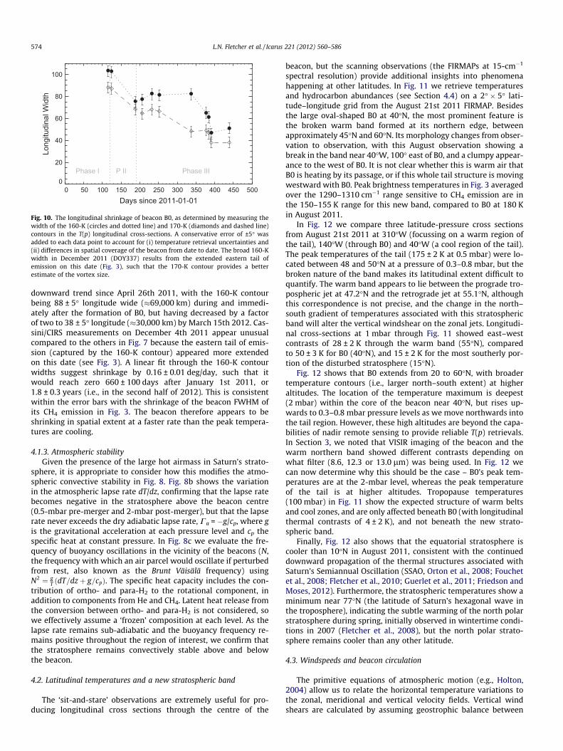
Despite this rather slow decline of the peak temperatures, themorphology of the beacon in Fig. 7 was changing, with thelongitudinal extent shrinking. If we arbitrarily select the 160 Kand 170 K contours, we can plot the width of B0 for each longitu-dinal cross-section (Fig. 10). Only dates with full coverage of thebeacon are included here, and a conservative error of ±5� has beenapplied to account for the confusion generated by the extendednortheastern ‘tail’ of the beacon. The two contours show a similar

0 50 100 150 200 250 300 350 400 450 500Days since 2011-01-01

0

20

40

60

80

100

Long

itudi

nal W

idth


Fig. 10. The longitudinal shrinkage of beacon B0, as determined by measuring thewidth of the 160-K (circles and dotted line) and 170-K (diamonds and dashed line)contours in the T(p) longitudinal cross-sections. A conservative error of ±5� wasadded to each data point to account for (i) temperature retrieval uncertainties and(ii) differences in spatial coverage of the beacon from date to date. The broad 160-Kwidth in December 2011 (DOY337) results from the extended eastern tail ofemission on this date (Fig. 3), such that the 170-K contour provides a betterestimate of the vortex size.


downward trend since April 26th 2011, with the 160-K contourbeing 88 ± 5� longitude wide (�69,000 km) during and immedi-ately after the formation of B0, but having decreased by a factorof two to 38 ± 5� longitude (�30,000 km) by March 15th 2012. Cas-sini/CIRS measurements on December 4th 2011 appear unusualcompared to the others in Fig. 7 because the eastern tail of emis-sion (captured by the 160-K contour) appeared more extendedon this date (see Fig. 3). A linear fit through the 160-K contourwidths suggest shrinkage by 0.16 ± 0.01 deg/day, such that itwould reach zero 660 ± 100 days after January 1st 2011, or1.8 ± 0.3 years (i.e., in the second half of 2012). This is consistentwithin the error bars with the shrinkage of the beacon FWHM ofits CH4 emission in Fig. 3. The beacon therefore appears to beshrinking in spatial extent at a faster rate than the peak tempera-tures are cooling.

4.1.3. Atmospheric stabilityGiven the presence of the large hot airmass in Saturn’s strato-

sphere, it is appropriate to consider how this modifies the atmo-spheric convective stability in Fig. 8. Fig. 8b shows the variationin the atmospheric lapse rate dT/dz, confirming that the lapse ratebecomes negative in the stratosphere above the beacon centre(0.5-mbar pre-merger and 2-mbar post-merger), but that the lapserate never exceeds the dry adiabatic lapse rate, Ca = �g/cp, where gis the gravitational acceleration at each pressure level and cp thespecific heat at constant pressure. In Fig. 8c we evaluate the fre-quency of buoyancy oscillations in the vicinity of the beacons (N,the frequency with which an air parcel would oscillate if perturbedfrom rest, also known as the Brunt Väisälä frequency) usingN2 ¼ g

T ðdT=dzþ g=cpÞ. The specific heat capacity includes the con-tribution of ortho- and para-H2 to the rotational component, inaddition to components from He and CH4. Latent heat release fromthe conversion between ortho- and para-H2 is not considered, sowe effectively assume a ‘frozen’ composition at each level. As thelapse rate remains sub-adiabatic and the buoyancy frequency re-mains positive throughout the region of interest, we confirm thatthe stratosphere remains convectively stable above and belowthe beacon.

4.2. Latitudinal temperatures and a new stratospheric band

The ‘sit-and-stare’ observations are extremely useful for pro-ducing longitudinal cross sections through the centre of the

beacon, but the scanning observations (the FIRMAPs at 15-cm�1

spectral resolution) provide additional insights into phenomenahappening at other latitudes. In Fig. 11 we retrieve temperaturesand hydrocarbon abundances (see Section 4.4) on a 2� � 5� lati-tude–longitude grid from the August 21st 2011 FIRMAP. Besidesthe large oval-shaped B0 at 40�N, the most prominent feature isthe broken warm band formed at its northern edge, betweenapproximately 45�N and 60�N. Its morphology changes from obser-vation to observation, with this August observation showing abreak in the band near 40�W, 100� east of B0, and a clumpy appear-ance to the west of B0. It is not clear whether this is warm air thatB0 is heating by its passage, or if this whole tail structure is movingwestward with B0. Peak brightness temperatures in Fig. 3 averagedover the 1290–1310 cm�1 range sensitive to CH4 emission are inthe 150–155 K range for this new band, compared to B0 at 180 Kin August 2011.

In Fig. 12 we compare three latitude-pressure cross sectionsfrom August 21st 2011 at 310�W (focussing on a warm region ofthe tail), 140�W (through B0) and 40�W (a cool region of the tail).The peak temperatures of the tail (175 ± 2 K at 0.5 mbar) were lo-cated between 48 and 50�N at a pressure of 0.3–0.8 mbar, but thebroken nature of the band makes its latitudinal extent difficult toquantify. The warm band appears to lie between the prograde tro-pospheric jet at 47.2�N and the retrograde jet at 55.1�N, althoughthis correspondence is not precise, and the change in the north–south gradient of temperatures associated with this stratosphericband will alter the vertical windshear on the zonal jets. Longitudi-nal cross-sections at 1 mbar through Fig. 11 showed east–westcontrasts of 28 ± 2 K through the warm band (55�N), comparedto 50 ± 3 K for B0 (40�N), and 15 ± 2 K for the most southerly por-tion of the disturbed stratosphere (15�N).

Fig. 12 shows that B0 extends from 20 to 60�N, with broadertemperature contours (i.e., larger north–south extent) at higheraltitudes. The location of the temperature maximum is deepest(2 mbar) within the core of the beacon near 40�N, but rises up-wards to 0.3–0.8 mbar pressure levels as we move northwards intothe tail region. However, these high altitudes are beyond the capa-bilities of nadir remote sensing to provide reliable T(p) retrievals.In Section 3, we noted that VISIR imaging of the beacon and thewarm northern band showed different contrasts depending onwhat filter (8.6, 12.3 or 13.0 lm) was being used. In Fig. 12 wecan now determine why this should be the case – B0’s peak tem-peratures are at the 2-mbar level, whereas the peak temperatureof the tail is at higher altitudes. Tropopause temperatures(100 mbar) in Fig. 11 show the expected structure of warm beltsand cool zones, and are only affected beneath B0 (with longitudinalthermal contrasts of 4 ± 2 K), and not beneath the new strato-spheric band.

Finally, Fig. 12 also shows that the equatorial stratosphere iscooler than 10�N in August 2011, consistent with the continueddownward propagation of the thermal structures associated withSaturn’s Semiannual Oscillation (SSAO, Orton et al., 2008; Fouchetet al., 2008; Fletcher et al., 2010; Guerlet et al., 2011; Friedson andMoses, 2012). Furthermore, the stratospheric temperatures show aminimum near 77�N (the latitude of Saturn’s hexagonal wave inthe troposphere), indicating the subtle warming of the north polarstratosphere during spring, initially observed in wintertime condi-tions in 2007 (Fletcher et al., 2008), but the north polar strato-sphere remains cooler than any other latitude.

4.3. Windspeeds and beacon circulation

The primitive equations of atmospheric motion (e.g., Holton,2004) allow us to relate the horizontal temperature variations tothe zonal, meridional and vertical velocity fields. Vertical windshears are calculated by assuming geostrophic balance between

(b) Temperature at 2 mbar [K]

360 315 270 225 180 135 90 45 0


20

40

60La

titud

e

140

160

180

(a) Temperature at 0.5 mbar [K]

360 315 270 225 180 135 90 45 0System III West Longitude

20

40

60

Latit

ude

140

150

160

170

(c) Temperature at 100 mbar [K]


20

40

60

Latit

ude

85

90

95

(d) Zonal Winds at 2 mbar [m/s]


20

40

60

Latit

ude

-300-200-100

0100200300

(e) Meridional Winds at 2 mbar [m/s]


20

40

60

Latit

ude

-200

-100

0

100

200

(f) Wind Magnitude at 2 mbar [m/s]


20

40

60

Latit

ude

0

100

200

300

400

(g) C2H2 at 2 mbar [ppm]


20

40

60

Latit

ude

0.20.40.60.81.01.21.4

(h) C2H6 at 2 mbar [ppm]

360 315 270 225 180 135 90 45 0


20

40

60

Latit

ude

2468

1012

Fig. 11. Horizontal variations of beacon properties during the mature phase III, retrieved from 15-cm�1 spectral resolution mapping observations on August 21st 2011. Panelsa–c show retrieved temperatures at the 0.5-, 2- and 100-mbar levels. Panels d and e show the calculated stratospheric winds from an integration of the thermal windshearequations. Panel f computes the magnitude of the winds (

ffiffiffiffiffiffiffiffiffiffiffiffiffiffiffiffiffiu2 þ v2p

) showing the peripheral collar of the vortex. Panels g and h show the spatial distribution of acetylene andethane at 2 mbar. The key for each panel is shown to its right.


Temperature Difference

80 75 70 65 60 55 50 45 40 35 30 25 20 15 10 5Planetographic Latitude

1.0000

0.1000

0.0100

0.0010

0.0001

Pres

sure

(bar

)

-2

-2

-2

-2

66

6

6

Zonal Temperatures (2009-11-04)


1.0000

0.1000

0.0100

0.0010

0.0001

Pres

sure

(bar

)

9090

90

90

100100

100100

110110

110110

120120

120

120

130

130

130

140

80 100 120 140 160 180


80 75 70 65 60 55 50 45 40 35 30 25 20 15 10 5

Planetographic Latitude

1.0000

0.1000

0.0100

0.0010

0.0001

Pres

sure

(bar

)

9090

9090

100100

100100

110110

110110

120120

120120

130130

130

130

140

140

150

150

160



1.0000

0.1000

0.0100

0.0010

0.0001

Pres

sure

(bar

)

-2

6

66

66

14

14

22

30



1.0000

0.1000

0.0100

0.0010

0.0001

Pres

sure

(bar

)

809090

9090

100100

100 100

110110

110 110

120120

120120

130130

130

130

140 150


80 75 70 65 60 55 50 45 40 35 30 25 20 15 10 5


1.0000

0.1000

0.0100

0.0010

0.0001

Pres

sure

(bar

)

90

90

9090

100100

100

100

110110

110110

120120

120

120

130130

130

130

140

140

150

150160

160

170

170

180

190


80 75 70 65 60 55 50 45 40 35 30 25 20 15 10 5


1.0000

0.1000

0.0100

0.0010

0.0001

Pres

sure

(bar

)

-2

6 6

6

6

6

14

14

14

22

2222

30

30

38

38

46

54

0 20 40 6080 100 120 140 160 180Δ

Fig. 12. The latitudinal variation of temperatures through the beacon, averaged over 10� of longitude at three different locations on August 21st 2011 (FIRMAP observation). Alatitude-pressure temperature cross-section from a 2009 observation is shown at the top of the figure for comparison. The three rows beneath represent longitudes of 310,140 and 40�W, through the beacon tail, the centre of B0, and the cold region to its east in Fig. 3, respectively. On the left we show the zonal temperatures, and on the right weshow the temperature difference compared to the 2009 observation. The same temperature scale is used for all similar plots. (For interpretation of the references to colour inthis figure legend, the reader is referred to the web version of this article.)



the meridional pressure gradients and Coriolis forces. In log-pres-sure coordinates, the thermal windshear equations for the zonal(u) and meridional (v) directions are:

f@u

@ lnðpÞ ¼Ra@T@w¼ R

@T@y

ð2Þ

f@v

@ lnðpÞ ¼ �R

a cos w@T@/¼ �R

@T@x

ð3Þ

where T is the temperature in Kelvin; p is the pressure in bar; f isthe Coriolis parameter f = 2Xsin(w) (where X is the planetary angu-lar velocity, w is the latitude); a is the mean planetary radius; / isthe longitude and R is the molar gas constant divided by the meanmolar weight of Saturn’s atmosphere. If we take 400 m/s as theperipheral velocity U (Fig. 11), and 50� longitude (approximately40,000 km) as a mean length scale L, then the Rossby number(Ro = U/fL) is �0.05, small enough that geostrophy is maintainedwithin the beacon.

The horizontal variation of the zonal and meridional strato-spheric winds is presented in Fig. 11d–f at 2 mbar for the AugustFIRMAP. If we assume the tropospheric zonal wind field of Sán-chez-Lavega et al. (2000) is referenced to the 500-mbar level, thenthese vertical windshears serve to accelerate zonal velocities at the2-mbar level that exceed 300 m/s at both the northern (prograde,largest dT/dy between 48 and 50�N) and southern (retrograde, larg-est dT/dy between 23 and 25�N) boundaries of B0 (Fig. 11). In themeridional direction, we assume a level of no motion at the tropo-pause, and integrating the windshear equations produces 2-mbarnorthward velocities of v > 200 m/s at the western boundary(175�W) and southward velocities of v < �200 m/s at the easternboundary (110�W). Taken together, the peripheral velocities inFig. 11 suggest a clockwise circulation around B0, with the largestmagnitude (�400 m/s) in a collar surrounding the vortex core,making this an anticyclone in the northern hemisphere. In this cal-culation, the meridional velocities appear to be smaller than thezonal velocities, something also observed in the circulation of Jupi-ter’s Great Red Spot (Choi et al., 2007), where maximum tangentialvelocities of 170 m/s were measured in the collar. To confirm therotation of the vortex, the relative vorticity, a measure of the localrotation in the fluid (the curl of the velocity field) is calculated asf = dv/dx � du/dy. Considering Fig. 11, we can see that dv/dx (westto east) is strongly negative and du/dy (south to north) is positive,resulting in an overall negative (i.e., anticyclonic) relative vorticitywithin the beacon.

The meridional velocities before the storm, pre-merger andpost-merger are compared in Fig. 13. When we calculate themeridional velocities for the March 4th 2011 COMPSIT observation,which captured both B1 and B2, we find 1-mbar meridional veloc-ities for B2 of 140 m/s northward at 280�W and 80 m/s southwardat 250�W, and for B1 we find 80 m/s northward at 130�W and70 m/s southward at 110�W (Fig. 14). The location of the maximumdT/dx varies with height, as suggested by the longitudinal temper-ature cross-section in Fig. 7, but this result suggests that the twooriginal beacons, B1 and B2, were anticyclonic vortices some20–30� wide with peripheral clockwise velocities of 70–140 m/s(the broad range represents the large uncertainties associated withextrapolating the thermal winds to stratospheric altitudes, assum-ing a level of zero meridional motion at 100 mbar). Fig. 14 showsthat the peripheral velocities around the combined B0 were greaterat the 1-mbar level than the individual beacons in March 2011,consistent with the downward shift of the peak temperatures from0.5-mbar to 2 mbar after the merger.

Finally, we investigate the zonal wind shear introduced by thepresence of the new warm stratospheric band at 48–50�N. If wecompute the zonal winds using a north–south cross-section at310�W (i.e., through the beacon tail but not the main vortex,

Fig. 11), we find prograde accelerations (80–120 m/s) at 52�Nand 60�N and a retrograde acceleration (120–160 m/s at 47�N) at1-mbar, bounding the tail of emission. Thus the new warm bandat the northern edge of B0 could be associated with zonal jets inthe stratosphere, prograde poleward of the new warm band andretrograde on the equatorward side, provided some process is ableto transport momentum (either by advection or eddy fluxes) intothese stratospheric jets.

4.4. Compositional variability

The peripheral jets surrounding the stratospheric anticycloneraise the possibility that the air mass within B0 is isolated fromthe ambient stratosphere, permitting unique environmental condi-tions. As described in Section 2.4, we varied the molecular abun-dances of ethane (C2H6) and acetylene (C2H2) as we retrieved thevertical T(p). This simultaneous fitting of temperatures and hydro-carbons gave slightly closer fits to the ethane and acetylene bandsthan a two-stage process, as the T(p) derived from the CH4 band re-quired minor adjustment within the retrieval uncertainties toreproduce the hydrocarbon emission. As their photochemical life-times are long relative to the lifetime of the storm, spatial varia-tions in hydrocarbon mixing ratios can be used to infer thetimescales for vertical transport by mixing in the stratosphere(e.g., Moses and Greathouse, 2005). In this study we make no at-tempt to derive the details of the vertical profiles of these species,but we retrieve a simple scaling factor for an a priori profile basedon mean hydrocarbon distributions from Cassini/CIRS limb analy-ses (Guerlet et al., 2009). In this way we can show trends in themolecular abundances, but we avoid issues related to non-overlap-ping contribution functions from CH4, C2H2 and C2H6 emission fea-tures (see Section 2.4).

4.4.1. AcetyleneIn Fig. 15, we use two techniques to show the variation of C2H2

with longitude and time – a cascade plot on the upper panel, witheach successive date offset by 2 ppm, and a comparison plot in thelower panel (for post-merger only), with the beacon shifted to180�W for all dates. On January 2nd 2011 we detect a contrast of0.1 ppm between the storm core and the adjacent beacons at310� and 230�W, at the level of the uncertainties on the retrievedabundance. This had increased by January 20th 2011, where B2(260�W) was enhanced in acetylene compared to adjacent longi-tudes by around a factor of two (the cold tropospheric anticyclonewas near 315�W on this date).

Variability in C2H2 is better shown in Fig. 16a, where we usedcoadded spectra of the individual beacons on each date to deter-mine the abundance of C2H2 in their centres. Pre-merger, we foundthat B1 and B2 had peak abundances of 0.8 ppm at 1 mbar (March4th 2011), and continued to grow (Fig. 16a), reaching a peak abun-dance of 1.6 ppm at 1 mbar on May 5th, shortly after the merger.Post-merger, the trends in Figs. 15 and 16a are more complex, withno obvious decline in the beacon abundance, remaining enhancedby a factor of three over quiescent conditions. Fig. 11g maps theC2H2 distribution in August 2011, showing it to be uniformly en-hanced within the boundary defined by the peripheral high-veloc-ity collar. During the mature phase, the abundance varies around amean of 1.3 ± 0.2 ppm (a factor of three greater than the typicalmean abundance of 0.4 ± 0.05 ppm at this latitude), but it is likelythat this variability is due to uncertainties arising from (i) inconsis-tent calibration between temporally separated CIRS observationsand (ii) slight differences in the latitudes and longitudes contribut-ing to the coadded spectra.

Longitudinal Temperatures (2011-08-21)

360 320 280 240 200 160 120 80 40 0


1.0000

0.1000

0.0100

0.0010

0.0001

Pres

sure

(bar

)

809090

90

90

100100

100

100

110110

110

110

120120

120

120

130130

130

130

140

140

150

150

150

160

160170180

190

80 100 120 140 160 180

Meridional Winds (2011-03-04) (ms-1)

360 320 280 240 200 160 120 80 40 0


1.0000

0.1000

0.0100

0.0010

0.0001

Pres

sure

(bar

)

-130 -90

-90-90

-50

-50

-50

-50

-10

-10

-10

-10-10

-10

-10

-10

01-

-10

0330

30

30

30

30

077070 110110

110

051

150190 23

0


360 320 280 240 200 160 120 80 40 0System III West Longitude

1.0000

0.1000

0.0100

0.0010

0.0001

Pres

sure

(bar

)

9090

90 90

100100

100 100

110110

110 110

120120

120 120

130

130 130

140140



1.0000

0.1000

0.0100

0.0010

0.0001

Pres

sure

(bar

)

01-

-10

-10-10

-10-10-10

-10

01-

01-

01--10

-10-10 -1

0-1

0 -10

-10 -10

-10

-10

-10

-10

0330

30 03

30

30

30

30

30

03

70 011


360 320 280 240 200 160 120 80 40 0


1.0000

0.1000

0.0100

0.0010

0.0001

Pres

sure

(bar

)

052-

-210

-170 -1

30 -90

-50-50

-10

-10-10

-10

-10

-10

-10

-10

-10

-10

01-

01-

-10-10

-10

30

30 30

30

30

70 7001

1 051

091 230

-200 -100 0 100 200


360 320 280 240 200 160 120 80 40 0


1.0000

0.1000

0.0100

0.0010

0.0001

Pres

sure

(bar

)

90

90

90

90

100100

100100

110110

110110

120120

120120

130130

130130

140140

150 150

150

160 16

0

170 17

0180

180

Fig. 13. Meridional windspeeds (right) calculated from the thermal windshear relationship and the temperature fields (left) for pre-storm (November 2009), pre-merger(March 2011) and in the decay phase (August 2011), showing the evolution of the north–south wind fields and their variability with altitude. Errors in the estimated windsare substantial, as there is great uncertainty in the level of zero motion (here assumed to be 500 mbar). Spectra were coadded between 35� and 45�N. Dotted lines in the righthand plots indicate retrograde (i.e., southward velocities). (For interpretation of the references to colour in this figure legend, the reader is referred to the web version of thisarticle.)


-200

-100

0

100

200

Mer

idio

nal V

eloc

ity (m

/s)

Fig. 14. A comparison of meridional winds at the 1-mbar level from March 4th2011 (dashed line, B1 to the right, B2 to the left) and B0 on August 21st 2011 (solidline). Winds were calculated using the thermal windshear relation, assuming a levelof zero motion at the cloud top and using the horizontal thermal gradients dT/dx tointegrate in the vertical. Arrows show the sense of the rotation, northward in thepositive direction, indicating that all three features are anticyclonic. Spectra used todetermine the windshear were coadded between 35� and 45�N.


4.4.2. EthaneFigs. 17 and 16b use the same techniques for showing the evo-

lution of ethane. In general, the longitudinal distribution of ethaneis more erratic, with east–west variability even in the absence ofthe storm perturbations (e.g., January 2011). By January 20th2011, there are suggestions that ethane was enhanced within thebeacons, but the contrasts between the warm vortex and the coolersurroundings is much smaller than for acetylene. In May 2011,immediately post-merger, there was evidence that C2H6 was en-hanced to the east of B0. However, when we compare all observa-tions of ethane after this date in the bottom panel of Fig. 17, thereis little consistent evidence for a trend in the C2H6 abundance. Thisis confirmed by the spatial distribution of ethane in August 2011(Fig. 11h), which shows the lack of ethane enhancements. Finally,if we retrieve C2H6 from the coadded spectra on each date, the re-sults hint that ethane may be enhanced (7.5 ± 1.0 ppm) in the bea-con compared to the quiescent background (6.5 ± 0.5 ppm), but theretrieval uncertainties are large.

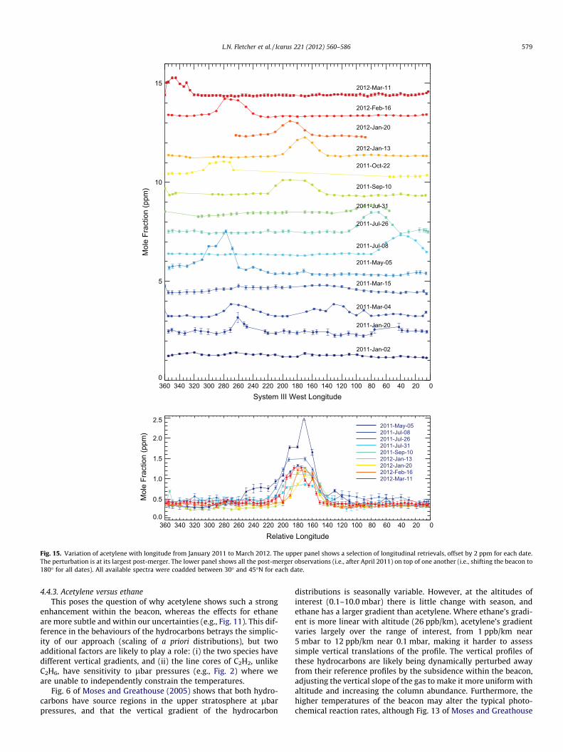
360 340 320 300 280 260 240 220 200 180 160 140 120 100 80 60 40 20 0System III West Longitude

0

5

10

15

Mol

e Fr

actio

n (p

pm)

2011-Jan-02

2011-Jan-20

2011-Mar-04

2011-Mar-15

2011-May-05

2011-Jul-08

2011-Jul-26

2011-Jul-31

2011-Sep-10

2011-Oct-22

2012-Jan-13

2012-Jan-20

2012-Feb-16

2012-Mar-11

360 340 320 300 280 260 240 220 200 180 160 140 120 100 80 60 40 20 0

Relative Longitude

0.0

0.5

1.0

1.5

2.0

2.5

Mol

e Fr

actio

n (p

pm)

2012-Mar-112012-Feb-162012-Jan-202012-Jan-132011-Sep-102011-Jul-312011-Jul-262011-Jul-082011-May-05

Fig. 15. Variation of acetylene with longitude from January 2011 to March 2012. The upper panel shows a selection of longitudinal retrievals, offset by 2 ppm for each date.The perturbation is at its largest post-merger. The lower panel shows all the post-merger observations (i.e., after April 2011) on top of one another (i.e., shifting the beacon to180� for all dates). All available spectra were coadded between 30� and 45�N for each date.


4.4.3. Acetylene versus ethaneThis poses the question of why acetylene shows such a strong

enhancement within the beacon, whereas the effects for ethaneare more subtle and within our uncertainties (e.g., Fig. 11). This dif-ference in the behaviours of the hydrocarbons betrays the simplic-ity of our approach (scaling of a priori distributions), but twoadditional factors are likely to play a role: (i) the two species havedifferent vertical gradients, and (ii) the line cores of C2H2, unlikeC2H6, have sensitivity to lbar pressures (e.g., Fig. 2) where weare unable to independently constrain the temperatures.

Fig. 6 of Moses and Greathouse (2005) shows that both hydro-carbons have source regions in the upper stratosphere at lbarpressures, and that the vertical gradient of the hydrocarbon

distributions is seasonally variable. However, at the altitudes ofinterest (0.1–10.0 mbar) there is little change with season, andethane has a larger gradient than acetylene. Where ethane’s gradi-ent is more linear with altitude (26 ppb/km), acetylene’s gradientvaries largely over the range of interest, from 1 ppb/km near5 mbar to 12 ppb/km near 0.1 mbar, making it harder to assesssimple vertical translations of the profile. The vertical profiles ofthese hydrocarbons are likely being dynamically perturbed awayfrom their reference profiles by the subsidence within the beacon,adjusting the vertical slope of the gas to make it more uniform withaltitude and increasing the column abundance. Furthermore, thehigher temperatures of the beacon may alter the typical photo-chemical reaction rates, although Fig. 13 of Moses and Greathouse

(a) Acetylene at 1 mbar

0 50 100 150 200 250 300 350 400 450 500Days since 2011-01-01

0.0

0.5

1.0

1.5

2.0

Mol

e Fr

actio

n [p

pm]


(b) Ethane at 1 mbar

0 50 100 150 200 250 300 350 400 450 500

Days since 2011-01-01

4

5

6

7

8

9

10

Mol

e Fr

actio

n [p

pm]


Fig. 16. Variation of the peak C2H2 (a) and C2H6 (b) abundances at 1 mbar for alldates sampled in Fig. 8. The dot-dash line shows the mean abundance at 40�N forquiescent longitudes. The dotted lines pre- and post-merger shows the meanabundances during these periods, with the dashed line showing the standarddeviations.


(2005) demonstrates that the gradients of the hydrocarbon profileshave a limited sensitivity to the stratospheric temperatures (theyare more sensitive to the seasonal variation of solar flux, for exam-ple). It is also interesting to note that C2H2 is an important productof ethylene photolysis (e.g., Moses et al., 2000), another hydrocar-bon observed to be greatly enhanced within the beacon (Hesmanet al., 2012).

To address the second possibility, we attempted to fit the C2H2

emission by varying T(p) alone, keeping the abundance at theambient values. The double-peaked nature of the contributionfunction (Fig. 2) meant that the line cores could only be fitted bya second high-temperature beacon at lbar pressures, leaving anambiguity between temperature and C2H2 abundance that cannotbe resolved by CIRS (the CH4 band used for temperature soundingis only sensitive to mbar pressures). The CH4 band fits cannot fullyrule out heating at lbar pressures and above as an alternative tothe enhancement of C2H2. A resolution of these questions mustawait sounding of the vertical profiles via higher-spectral resolu-tion datasets (e.g., those acquired by Hesman et al. (2012) andGreathouse et al. (2011)).

4.5. Absence from reflected sunlight observations

One puzzle concerning the hot stratospheric temperatures isthe apparent absence of any effects in reflected sunlight, implyingthat the anticyclonic vortex is (i) having no effect on the tropo-spheric cloud decks; and (ii) no effects on the haze materials inthe upper troposphere and lower stratosphere. To investigate thisfurther, a full Cassini/VIMS 0.8–5.1 lm cube covering the beaconlongitude on July 12th 2011 (63–18�W at a latitude of 15�N, withwider longitude coverage at more northerly latitudes) was pro-vided by K. Baines and T. Momary (private communication). The

cube was acquired at 21:54 UT on July 12th 2011 (number1689201784). We found no structures in the clouds and hazes cor-responding to the beacon, focussing on the strongly-absorbingbands to sense the lower stratospheric hazes. The most prominentfeature was the low-reflectivity band between 25� and 45�N left inthe wake of the storm. Indeed, there was nothing notable about thebeacon longitude in reflected sunlight in the VIMS cubes.

We can also compare to Cassini/ISS data obtained on July 12th2011 (Fig. 9 of Sayanagi et al. (2012)), which also covers a completelongitude circle. Their false-colour maps use a combination of CB2–MT2–MT3 filters, with methane filters probing upper-level hazes.Although the storm latitude band is replete with small-scale vorti-ces and eddies, there is nothing notable about the beaconlongitude.

Finally, we alerted the amateur community to the beacon longi-tudes throughout 2011 and 2012, to assess whether small-scaleclouds and spots were more prevalent at the beacon longitudesthan elsewhere. Submissions were received from T. Barry, A. Wes-ley, C. Go, P. Haese and M. Delacroix, and we continued to surveythe Planetary Virtual Observatory Database (Hueso et al., 2010)for any signs of unusual activity. However, at the time of writing,we conclude that the hot stratospheric temperatures are havingno effect on the clouds and hazes at higher pressures, and cannotbe viewed in reflected sunlight. The most prominent feature inthe visible, however, was the new white axisymmetric band be-tween 45� and 50�N that had formed in the aftermath of the storm.The southern edge of this band was undulating with waves, corre-sponding to the continued churning of the storm band. In March2012, this bright reflective band sits north of the low-reflectivitystorm latitudes observed by VIMS (25–45�N), but slightly southof the warm tail of beacon emission identified previously between50 and 60�N.

5. Discussion

The thermal-IR data have captured the formation, strengthen-ing, merger and decay phase of a large warm anticyclonic vortexin Saturn’s northern stratosphere that is invisible in reflected sun-light (see summary in Table 5). Taking the vortex width to be de-fined by the maximal east–west temperature gradients, dT/dx, wefind that the beacon was some 50,000 km wide in August 2011(Fig. 11), a factor of two larger than Jupiter’s Great Red Spot. In thissection we discuss theories for the origins, nature and motion ofthis new stratospheric vortex.

5.1. Beacon origins

The tropospheric storm started in the vicinity of Saturn’s firstretrograde jet north of the equator at 39.2�N. These westwardmid-latitude jets have been previously identified as sites of poten-tial barotropic instability (Read et al., 2009; Achterberg and Flasar,1996), leading to interesting dynamical phenomena and eddyactivity derived from the mean zonal flow. For example, this is alsothe latitude of Saturn’s string of pearls, a chain of small cloud-freevortices first identified in 5-lm emission (Momary et al., 2006). In-deed, Sayanagi et al. (2012) suggest that the eruption occurredwithin the pearl features themselves. In the southern hemisphere,the first retrograde jet at 40.7�S is associated with the string ofsmall-scale convective clouds and vortices known as storm alley.However, never before have these tropospheric perturbations pro-duced detectable perturbations to Saturn’s stratospheric emission.

Reflected sunlight observations of the tropospheric cloud deckare consistent with the disturbance being initiated as a convectivestorm (or multiple convective plumes) driven by the condensationof water (Sánchez-Lavega et al., 2011; Fischer et al., 2011). The

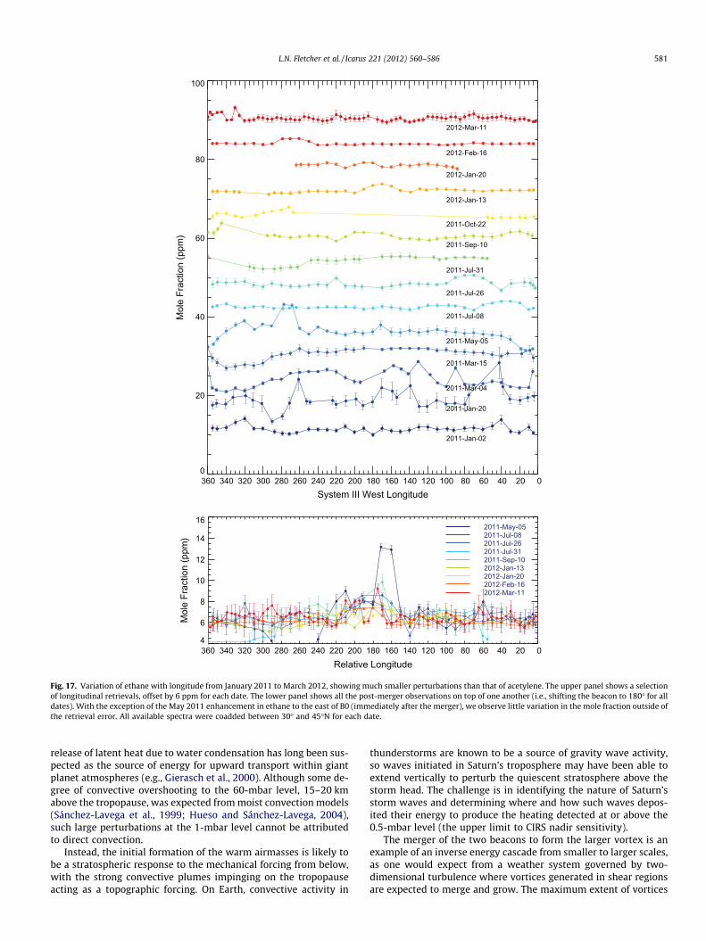
360 340 320 300 280 260 240 220 200 180 160 140 120 100 80 60 40 20 0System III West Longitude

0

20

40

60

80

100

Mol

e Fr

actio

n (p

pm)

2011-Jan-02

2011-Jan-20

2011-Mar-04

2011-Mar-15

2011-May-05

2011-Jul-08

2011-Jul-26

2011-Jul-31

2011-Sep-10

2011-Oct-22

2012-Jan-13

2012-Jan-20

2012-Feb-16

2012-Mar-11

360 340 320 300 280 260 240 220 200 180 160 140 120 100 80 60 40 20 0

Relative Longitude

4

6

8

10

12

14

16

Mol

e Fr

actio

n (p

pm)

2012-Mar-112012-Feb-162012-Jan-202012-Jan-132011-Sep-102011-Jul-312011-Jul-262011-Jul-082011-May-05

Fig. 17. Variation of ethane with longitude from January 2011 to March 2012, showing much smaller perturbations than that of acetylene. The upper panel shows a selectionof longitudinal retrievals, offset by 6 ppm for each date. The lower panel shows all the post-merger observations on top of one another (i.e., shifting the beacon to 180� for alldates). With the exception of the May 2011 enhancement in ethane to the east of B0 (immediately after the merger), we observe little variation in the mole fraction outside ofthe retrieval error. All available spectra were coadded between 30� and 45�N for each date.


release of latent heat due to water condensation has long been sus-pected as the source of energy for upward transport within giantplanet atmospheres (e.g., Gierasch et al., 2000). Although some de-gree of convective overshooting to the 60-mbar level, 15–20 kmabove the tropopause, was expected from moist convection models(Sánchez-Lavega et al., 1999; Hueso and Sánchez-Lavega, 2004),such large perturbations at the 1-mbar level cannot be attributedto direct convection.

Instead, the initial formation of the warm airmasses is likely tobe a stratospheric response to the mechanical forcing from below,with the strong convective plumes impinging on the tropopauseacting as a topographic forcing. On Earth, convective activity in

thunderstorms are known to be a source of gravity wave activity,so waves initiated in Saturn’s troposphere may have been able toextend vertically to perturb the quiescent stratosphere above thestorm head. The challenge is in identifying the nature of Saturn’sstorm waves and determining where and how such waves depos-ited their energy to produce the heating detected at or above the0.5-mbar level (the upper limit to CIRS nadir sensitivity).

The merger of the two beacons to form the larger vortex is anexample of an inverse energy cascade from smaller to larger scales,as one would expect from a weather system governed by two-dimensional turbulence where vortices generated in shear regionsare expected to merge and grow. The maximum extent of vortices


typically depends on the width of the belt or zone in which theyare embedded, but the abnormally large size of the stratosphericanticyclone, cutting across jet streams at 32�, 39�, 47� and 55�N,hints at a different regime of zonal motion in the high stratosphere.The reasons for the downward shift in the beacon post-merger, by1.4 scale heights, and the associated enhancement in temperaturesand acetylene abundances, are not understood.

5.1.1. Numerical simulationGiven previous successes in reproducing the storm morphology

at Saturn’s cloud tops with non-linear simulations (e.g., Sánchez-Lavega et al., 2011), and in particular the tropospheric cold anticy-clonic vortex observed by Fletcher et al. (2011), we attempted tosimulate beacon formation using the EPIC atmospheric model (ex-plicit planetary isentropic-coordinate, Dowling et al., 1998). EPIC isa primitive-equation model, and fully includes production of Ross-by waves, Kelvin waves and gravity waves by the storm head,although modelling their properties correctly remains a challenge.The reference T(p) from Section 2.4 was divided into 10 verticallayers (isentropic surfaces) between approximately 0.01 mbarand 10 bar. A steady vertical Gaussian heat source exists forp > 200 mbar to mimic the powerful convective activity of thestorm head (lowest three layers of the model), whose vertical ex-tent, horizontal width and intensity can be varied (nominal inten-sity of 1000 W/m2). This heat source is an intense source of gravitywaves, which propagate outwards in three dimensions, horizon-tally and vertically through the stably-stratified upper atmosphere.However, the waves were reflected at the boundaries of the do-main (despite the use of ‘sponge layers’ in the top two layers ofthe model) and result in temperature maps by day 30 that weredominated by noise and bore no resemblance to the Cassini mea-surements. EPIC cannot provide information on where these wavesultimately deposit their energy, a limitation of the horizontal andvertical domain ranges selected to allow for reasonable computa-tional efficiency.

The natural output of EPIC are maps of potential vorticity (PV),which can be considered as a passive tracer of the dynamics. Oursimulations confirmed that tropospheric activity can produce per-turbations to PV distributions at stratospheric altitudes, but themorphology of the PV field at 1 mbar is extremely sensitive tothe chosen vertical windshear, du/dz, which is poorly constrainedby measurements (see Appendix A). Simulations often producedlarge-scale stratospheric airmasses with anticyclonic vorticity(reminiscent of B1) in the vicinity of the upwelling and divergenceover the tropospheric storm head. However, definitive conclusionsare not possible due to the sensitivity to the chosen u(z); the lim-ited domain size and gravity wave internal reflections; and thecoarse nature of the vertical grid. Improvements of these simula-tions will be the subject of future research.

5.1.2. Relationship to planetary wavesOne possible interpretation of the beacon origins is that they

were formed as topographically-forced Rossby waves due to thepowerful tropospheric convection. Charney and Drazin (1961)demonstrated that the vertical propagation of planetary wave dis-turbances from the troposphere (caused by mechanical forcingfrom instabilities) depends on the effective index of refraction ofthe waves, and hence on the variation of the mean zonal wind withaltitude. On Earth, strong Rossby-wave disturbances in the strato-sphere are frequently due to upward propagation of waves gener-ated by large-scale weather disturbances in the troposphere (e.g.,Andrews et al., 1987). Non-linear vertical eddy transports of heatand momentum associated with these waves could then modifythe basic zonal flow and produce the stratospheric perturbationswe see. When the flow is prograde, the atmosphere acts as ashort-wave filter and only the longest wavelengths of Rossby waves

can propagate vertically, meaning that the stratospheric distur-bances are large in scale. Achterberg and Flasar (1996) previouslyidentified 37–41�N as a critical region where the potential vorticitygradient vanishes and instabilities could excite Rossby waves.

Rossby waves owe their existence to the change in Coriolis forcewith latitude (known as the b effect, where b = df/dy = 2Xcosw/R,fis the Coriolis parameter 2Xsinw, w is the latitude; R is the plane-tary radius and X is the planetary rotation velocity), which acts asa restoring force for parcels displaced meridionally. In a three-dimensional atmosphere, the zonal phase speed c relative to themean zonal wind u is given by (Sánchez-Lavega, 2011):

u� c ¼ b

k2 þ l2 þ f 20 =N2

B

� �ðm2 þ 1=4H2Þ

ð4Þ

Here k, l and m are the zonal, meridional and vertical wavenumbers,respectively; H is the atmospheric scale height (50.2 km for the lat-itude and altitude of the beacon); and NB is the Brunt Väisälä fre-quency (considered to be constant at 7 � 10�3 s�1 at the altitudesof the beacons). The Coriolis parameter is f0(40�) = 2.1 � 10�4 andb(40�) = 4.3 � 10�12 m�1 s�1.

Crucial to the case of the beacons is whether the Rossby wavescan propagate vertically from their tropospheric source, requiringthat the vertical wavenumber m is real and non-zero (i.e.,m2 > 0), which implies that the quantity u � c must be less thansome critical velocity for vertical propagation, Uc, given by (Sán-chez-Lavega, 2011):

Uc ¼b

k2 þ l2 þ f 20 =4H2N2

B

ð5Þ

Evaluation of this expression requires a selection of the relevanthorizontal sizes. The zonal wavenumber, k = 2p/Lx, depends on theselected east–west dimension Lx – the width of B0 (some 70� atits largest), or the horizontal separation of B1 and B2 (extrapolatedto be 39� in Section 3 at the time of the storm outbreak, but increas-ing as the two beacons moved apart). The meridional wavenumber,l = 2p/Ly, assumes a north–south distance of 30� latitude, with lati-tudinal extent of the beacon. Taking 39–70� as a suitable range forLx, we find critical velocities in the range Uc = 24–30 m/s. Evenassuming a wave of 360� horizontal extent, the largest value we ob-tain for Uc is 32.5 m/s. To assess the vertical propagation, we mustdetermine the ambient zonal velocity at the altitude of the beacon(see Appendix A), which is expected to vary with season. FromFig. 11d, the beacon is centred in a band where the 2-mbar veloci-ties appear close to zero away from the beacon itself, althoughuncertainties are large and the dT/dy at this latitude may alreadyhave been affected by the storm before August 2011. This wouldimply that u � c � 25 m/s < Uc (as c � � 25 m/s), satisfying the con-dition for the vertical propagation of Rossby wave disturbances ofthis horizontal size and drift rate.

However, we caution that the variation of the zonal wind withlatitude on the giant planets implies that we should replace b witha modified value which includes the effects of the meridionalcurvature of the zonal winds (note that we do not account for ver-tical curvature of the winds in this calculation). If we replace b byan effective be ¼ b� @2u

@y2, we find that be is negative at 40�N becausethe second derivative of the zonal velocity field is positive. Hencethe corresponding critical velocity Uc is retrograde and it is incon-clusive as to whether planetary waves are able to propagate up-wards from a tropospheric source. However, wave disturbancescould still enter this evanescent region, their amplitudes decayingaway from the source but potentially leaking into the upper atmo-sphere (e.g., Achterberg and Flasar, 1996). In summary, a beaconorigin due to the vertical propagation of planetary waves fromthe tropospheric storm is supported by our simple calculations


(in addition to gravity waves), but more sophisticated modelling isrequired to confirm this interpretation.

5.2. Conditions within the stratospheric anticyclone

At first glance, the thought of a warm stratospheric hotspot as ananticyclone may be confusing. For example, both Jupiter’s Great RedSpot (GRS) and the anticyclone formed in Saturn’s troposphere bythe storm (Fletcher et al., 2011; Sánchez-Lavega et al., 2011) arecold-core features, with temperatures increasing radially outwardsleading to windshears that decelerate their anticyclonic motion. Onthe other hand, Saturn’s stratospheric anticyclone has temperaturesdecreasing radially outwards, accelerating its clockwise motionwith height. The tropospheric convective plumes served as a sourceof anticyclonic vorticity (implied by the upwelling and divergenceof material on a rotating planet), and this anticyclonicity was some-how transported vertically throughout the atmosphere, leading tothe clockwise rotation of the beacon at high altitude.

When the Rossby number is less than unity, angular momen-tum conservation on a rotating planet (the Coriolis effect) requiresthat high pressure systems are surrounded by clockwise winds tobalance the pressure gradient in the northern hemisphere – ananticyclone. On Earth we think of anticyclones (high pressure re-gions) as regions of subsiding, dry air, the opposite of what we findfor Jupiter’s GRS. In the free atmosphere, winds will flow parallel toisobars, but frictional forces on a solid surface causes air to crossisobars, leading to divergence at the base of a high-pressure system(i.e., the velocity has a component outwards from the centre). Toconserve the mass of air within the system, air therefore sinks overhigh pressure systems on Earth. In Saturn’s troposphere, the fric-tional damping responsible for the deceleration of the zonal windswith altitude occur at the upper boundary of the vortices (due tosome unidentified source of damping, e.g., Conrath and Pirraglia,1983), rather than at the bottom, which may explain why anticy-clones in giant planet tropospheres are regions of upwelling anddivergence at the top. But what of anticyclones in the strato-sphere? Here the situation may be reversed and more ‘Earth-like’,with friction at the lower boundary of the high-pressure systemcausing outflow at the bottom, and mass conservation resultingin atmospheric subsidence within the beacon.

The amount of energy required to heat up the stratospheric bea-con can be estimated from the August 2011 mapping observation.We calculate the energy density required at each pressure level toproduce the temperature difference DT(p) compared to the quies-cent background:

e ¼ 1mg

Z pmax

p0

CpðpÞDTðpÞdp ð6Þ

where e is the energy density per unit area, Cp(p) is the specific heatat constant pressure calculated for each pressure level, DT(p) is thetemperature perturbation, g is the local gravitational accelerationand m is the mean molecular weight. The integration was per-formed between 0.1 and 100 mbar. Summing this within the ovaldetermined by the peripheral vortex collar in Fig. 11, we estimatea total energy of 1021 J to produce this temperature perturbation,which is only a small fraction of (i) the 6.2 � 1024 J of energy emit-ted by Saturn in a single year (Hanel et al., 1983), and (ii) the esti-mated total energy of 1024 J released by lightning in the thunderstorm during its lifetime (Fischer et al., 2011).

6. Conclusions

The evolution of Saturn’s stratospheric vortex was describedusing spatial mapping of hydrocarbon emission and retrievals ofatmospheric temperatures, stability, winds and composition. Table

5 provides an overview of the key events in the vortex evolution,and here we summarise some of the key findings of this study.

1. Thermal imaging and spectroscopy sensitive to hydrocarbonemission in Saturn’s stratosphere have revealed the never-before-seen stratospheric perturbations triggered by a plane-tary-scale tropospheric storm. The evolutionary sequence canbe divided into three phases: (I) the formation and intensifica-tion of two distinct warm airmasses between January and April2011; (II) the merging and deceleration to form the large singlebeacon between April and June 2011; and (III) the accelerationand slow cooling of the beacon since July 2011. One beacon (B1)was more extended, and located directly above the convectingstorm head in the troposphere, moving west at 2.73 ± 0.1 deg/day. The second beacon (B2) was more compact and at a moresoutherly latitude, moving west at 0.6 ± 0.1 deg/day. This differ-ence in drift rates caused the two beacons to encounter oneanother, when they behaved as two coherent anticyclonic vor-tices and merged in late April 2011, forming a single large bea-con complex (B0).

2. Beacon B0 was tracked in Saturn’s stratosphere from May 2011to March 2012, and persisted as the largest vortex detected inour Solar System to date (covering approximately 65� longitudebetween peripheral velocity peaks in August 2011, 50,000 km at39�N, and extending between 20�N and 60�N), containing thehottest temperatures measured to date (the maximum temper-ature retrieved was 221.6 ± 1.4 K at 2 mbar on May 5th 2011).B0 moved rather slowly (1.6 ± 0.2 deg/day) for the first twomonths post-merger, but then accelerated to 2.70 ± 0.04 deg/day (�24.5 ± 0.4 m/s at 39.5�N) where it remained for theremainder of the observing period. B0 had no association withthe tropospheric storm head after the merger, existing as anindependent phenomenon, a ‘free mode’ of the stratosphericcirculation. No perturbations to visible clouds and hazes weredetected during this period. B0 was accompanied by a warm tailof stratospheric emission with peak temperatures between 0.3–0.8 mbar and 48–50�N, generating stratospheric thermal winds-hears to accelerate a retrograde jet at 47�N and a prograde jet at52�N. The peak temperatures within the vortex are coolingslowly, by approximately 0.11 ± 0.01 K/day (40.2 ± 3.7 K/year,faster than the radiative time constant at 2 mbar for Saturn’snominal atmosphere), and the width of the 160-K contours isshrinking by 0.16 ± 0.01 deg/day. Both of these processes, cool-ing and shrinking, will ultimately return Saturn’s northernstratosphere to quiescent conditions.

3. Retrievals of atmospheric temperatures show that the mergerof B1 and B2 was associated with a downward shift in the peaktemperatures from 0.5 mbar pre-merger to 2 mbar post-merger,a translocation of approximately 1.4 scale heights. Such adownward shift partially explains the enhancement in the acet-ylene abundance by a factor of 3 within the vortex, but fails toexplain the lack of variability in stratospheric ethane. Despitethe negative lapse rate introduced into the stratosphere bythe presence of the beacon, calculations of the temperaturegradient confirm that the atmosphere above the beaconremains sub-adiabatic. Although the sensitivity of the CIRSnadir spectra is minimal above the 0.1-mbar level, the retrievalsdo hint at structure associated with the stratospheric distur-bance at even lower pressures, which could ultimately beexplored by higher-resolution spectroscopy.

4. Thermal windshear calculations allow us to analyse the veloci-ties of the vortex, confirming a Rossby number much smallerthan unity (hence geostrophy is maintained), and demonstrat-ing anticyclonic vorticity (clockwise rotation) with peripheralvelocities of 200–400 m/s at 2 mbar. The clockwise peripheralvelocities of the two original beacons was smaller (70–140 m/


s). The tropospheric storm, featuring upwelling and divergence,was a source of anticyclonic vorticity for the stratosphere.

5. Stratospheric acetylene at 2 mbar is uniformly enhanced withinperipheral high velocity collar by a factor of three compared tothe typical mean abundance of 0.4 ± 0.05 ppm at this latitude,varying around a mean of 1.3 ± 0.2 ppm, consistent with thedownward displacement of the vortex post-merger. Ethane var-iability is within our retrieval uncertainty. The differencesbetween the two hydrocarbons may be related to unusualchemistry within the hot vortex; differences in the vertical dis-tribution; or possible high-altitude structure (sensed by C2H2

line cores) that cannot be reliably measured by CIRS.6. The origins of the beacons remain uncertain, but numerical sim-

ulation shows that the tropospheric convective plumes imping-ing on the tropopause acted as strong source of waves (gravitywaves, planetary waves), which extend in three dimensionsaway from the source. The upward transmissivity of the waveactivity depends on the details of the temperature and windstructure near the tropopause, and simple calculations indicatethat vertical Rossby wave propagation was permitted duringthis springtime epoch. The energy and momentum transportedby these waves was deposited at stratospheric altitudes, andnon-linear effects caused the formation of the two vortices,transferring energy from smaller to larger scales (an exampleof an inverse energy cascade).

The mystery of why this storm and other planetary-scale distur-bances occur during Saturn’s northern spring and summer remainsunanswered. As seasonal changes to the vertical T(p) profile occuronly at altitudes above the 500–700 mbar level, the seasonal trig-gering of the disturbance at great depth is rather puzzling. How-ever, these seasonal changes may modify the circulation withinthe upper troposphere down to the topmost clouds, increasingthe convective conditions and thereby altering the meridional cir-culation beneath the clouds, permitting large convective eventsfrom below (that are themselves independent of season) to extendhigher than they could otherwise. This would suggest that themoist convective features could have been pre-existing (for exam-ple, Jupiter’s moist convective events occur almost randomly intime), but only when seasonal thermal changes occurred did thefull outbreak erupt.

This is the first time that the formation of a large stratosphericanticyclone, associated with a tropospheric convective storm, hasbeen observed on a giant planet. Jupiter’s north pole features a‘hot spot’ at 60�N that is a region of high UV, infrared and X-rayemission (Gladstone et al., 2002, and references therein), but thisis likely to be related to heating by auroral processes. Mid-latitudeconvective storms on Jupiter have been monitored in thermal-IRimaging (e.g., Sánchez-Lavega et al., 2008), but to date there havebeen no detections of stratospheric heating, making Saturn’sstratospheric anticyclone unique. Stratospheric anticyclones arecommon features of the Earth’s stratosphere, most common innorthern winter and southern spring (Harvey and Hitchman,1996; Harvey et al., 2004), and possibly associated with upwardextension of planetary waves from tropospheric sources (e.g., Char-ney and Drazin, 1961). Their growth and intensification oftenaccompanies the distortion and displacement of the polar cyclonicvortices from the poles (e.g., the Aleutian high displacing the Arcticvortex and the Australian high displacing the Antarctic vortex) andare associated with sudden stratospheric warming events (e.g., An-drews et al., 1987). On Earth, stratospheric anticyclones are regionsof strong gradients in potential vorticity and trace species (e.g.,Manney et al., 1995), just as Saturn’s vortex appears to be entrain-ing a region of elevated C2H2.

These thermal-IR observations demonstrate the strong couplingover hundreds of kilometres between the tropospheric outburst

and the stratospheric thermal structure. It is not known whetherprevious saturnian storms produced similar stratospheric pertur-bations, or whether they will in future. Many of the physical pro-cesses revealed by this infrared study will require numericalmodelling to explore in greater detail, such as those processesresponsible for (i) transporting energy into the stratosphere fromthe tropospheric perturbation; (ii) forming two warm airmassesat 0.5 mbar that moved at different velocities; (iii) merging thevortices and translating the peak temperatures down by 1.7 scaleheights; and (iv) maintaining B0 as a large anticyclone, stableagainst dissipative effects over long time periods. The ultimate fateof Saturn’s unique stratospheric vortex remains to be seen, andnew convective storms during Saturn’s northern summer (startingin May 2017) will be intensively studied to determine whether thiswill phenomenon will happen again.

Acknowledgments

Fletcher was supported by a Glasstone Science Fellowship at theUniversity of Oxford. We thank the members of the Cassini/CIRSinvestigation team who have assisted in the design of the imagingsequences, instrument commands and other vital operationaltasks, and the Ground Systems Operations for the Cassini Project.We wish to thank the directors and staff of the ESO Very LargeTelescope and the NASA Infrared Telescope Facility for their assis-tance with the execution of these observations. This investigationwas partially based on observations acquired at the Paranal UT3/Melipal Observatory under ID 386.C-0096 and 287.C-5032. Pro-gram 386.C-0096(A) had been awarded time to study Saturn’s slowseasonal evolution in April 2011, but we are grateful to ESO forgranting our request to obtain these images of Saturn’s storm assoon as the planet became available after solar conjunction (whichoccurred in October 2010).

We are grateful to the operators at the NASA/Infrared TelescopeFacility (operated by the University of Hawaii under CooperativeAgreement No. NCC 5-538 with the National Aeronautics andSpace Administration, Science Mission Directorate, PlanetaryAstronomy Program). The UK authors acknowledge the supportof the Science and Technology Facilities Council (STFC). B.E.H.,G.L.B., and R.K.A. were supported by the NASA Cassini DataAnalysis Participating Scientists (CDAPS) Program Grant No.NNX12AC24G. GSO is supported by Grants from NASA to the JetPropulsion Laboratory, California Institute of Technology. J.L.,E.G.M. and A.S.L. were supported by the Spanish MICIIN ProjectAYA2009-10701 with FEDER funds, by Grupos Gobierno VascoIT-464-07 and by Universidad Pas Vasco UPV/EHU through pro-gram UFI11/55. We thank T. Greathouse and J. Moses for helpfuldiscussions of the beacon results.

Appendix A. Stratospheric zonal winds

Given the large number of mysteries surrounding this newstratospheric phenomenon, we investigated whether the presenceof a long-lived feature in Saturn’s stratosphere could have enableda direct measurements of stratospheric winds. If the beacons canbe truly considered as vortices or wave-like phenomena, their mo-tions would be determined by the types of waves responsible andthe background zonal velocity, u. However, the fact that B1 (andlater B0) moved with the same velocity as the tropospheric stormhead, despite a vertical separation of hundreds of kilometres, sug-gested a highly barotropic atmosphere, with little variation of theretrograde velocity with altitude. This is partially borne out byFig. 11d, which suggests zonal velocities near zero at 2 mbar inAugust 2011. However, the ambient zonal flow varies with time,which would have a significant effect on the trapping of planetary


waves in the troposphere (i.e., preventing the vertical propaga-tion). If we had taken mid-latitude zonal winds from Cassini’sprime mission (2004–2008 during northern winter), the 39.2�Njet, we find that the jet should switch from a retrograde velocityof �20 m/s at 500 mbar, to zero velocity near 150 mbar, thenincreasing to form a prograde jet of �100 m/s at 1 mbar, and plan-etary waves would have been trapped in the troposphere(u � c � 125 > Uc).

This large stratospheric velocity difference between wintertimeand springtime mid-latitudes prompted us to explore the effectson the vertical shear on the zonal winds due to Saturn’s seasonalasymmetry in temperatures (e.g., Friedson and Moses, 2012). Cas-sini observations since 2004 have revealed the slow variation ofstratospheric temperatures (Fletcher et al., 2007, 2010), which isreproduced by numerical modelling of the radiative response toinsolation changes. During southern summertime conditions atthe start of the Cassini observations, the thermal gradient dT/dywas largely negative, such that the northern winter hemispherehas a positive vertical shear, du/dz, accelerating the progradestratospheric flow as described above. The southern summerhemisphere had a corresponding negative vertical shear, promot-ing retrograde flow in the southern stratosphere. As the seasonsprogress into northern spring and summer by May 2017, the tem-perature asymmetry should reverse to a positive dT/dy, causing anegative vertical shear, du/dz, in the northern summer hemi-sphere. These simple arguments suggest that the direction of thestratospheric zonal flows are seasonally reversing, thus changingthe transmissivity of the lower stratosphere to Rossby wavepropagation.

We used the radiative climate model of Greathouse et al.(2008) (applied to Saturn by Fletcher et al. (2010)) to simulatethe changing hemispherical stratospheric dT/dy with time throughan entire saturnian year. The magnitude of the calculated zonalvelocity is highly sensitive to (i) the shielding effects of the rings(the model lacks advective motions, and therefore produces artifi-cially large cooling effects in the ring shadowed regions); (ii) themeridional distribution of stratospheric hydrocarbons, particularlyC2H2 and C2H6, which are held constant in the model; (iii) therange of latitudes over which we average the zonal wind field;and (iv) the assumed level of zero motion, here arbitrarily set tothe tropopause. The temperature predictions were used to calcu-late the vertical windshear with latitude and season, and thenaveraged over the 30–50�N range of the beacon. The model sug-gests that the magnitude of the prograde stratospheric flow hasbeen decreasing at 40�N for the majority of the Cassini mission,and it is not inconceivable that retrograde motion could havebeen in place in the stratosphere when the storm first erupted,as suggested by Fig. 11d. Conditions may have been ‘just right’for planetary wave propagation in Saturn’s springtime to formthe beacons. However, given the uncertainties associated withthe extrapolation of the thermal winds above the cloud tops, wemust await direct measurements of middle-atmospheric circula-tion to be certain of this temporal variability of stratosphericwinds.

References

Achterberg, R.K., Flasar, F.M., 1996. Planetary-scale thermal waves in Saturn’s uppertroposphere. Icarus 119, 350–369.

Andrews, D.G., Holton, J.R., Leovy, C.B., 1987. Middle Atmosphere Dynamics.Academic Press, New York.

Blass, W.E., Halsey, G.W., Jennings, D.E., 1987. Self- and foreign-gas broadening ofethane lines determined from diode laser measurements at 12 microns. J.Quant. Spectrosc. Radiat. Trans. 38, 183–184.

Borysow, A., Frommhold, L., 1986. Theoretical collision-induced rototranslationalabsorption spectra for the outer planets: H2–CH4 pairs. Astrophys. J. 304, 849–865.

Borysow, A., Frommhold, L., 1987. Collision-induced rototranslational absorptionspectra of CH4–CH4 pairs at temperatures from 50 to 300K. Astrophys. J. 318,940–943.

Borysow, J., Frommhold, L., Birnbaum, G., 1988. Collison-induced rototranslationalabsorption spectra of H2–He pairs at temperatures from 40 to 3000 K.Astrophys. J. 326, 509–515.

Bouanich, J.-P., Salem, J., Aroui, H., Walrand, J., Blanquet, G., 2004. H2-broadeningcoefficients in the m2 and m4 bands of PH3. J. Quant. Spectro. Rad. Trans. 84, 195–205.

Brown, L.R., Peterson, D.B., 1994. An empirical expression for linewidths ofammonia from far-infrared measurements. J. Mol. Spectrosc. 168, 593–606.

Brown, L.R. et al., 2003. Methane line parameters in HITRAN. J. Quant. Spectrosc.Radiat. Trans. 82, 219–238.

Charney, J.G., Drazin, P.G., 1961. Propagation of planetary-scale disturbances fromthe lower into the upper atmosphere. J. Geophys. Res. 66, 83–109.

Choi, D.S., Banfield, D., Gierasch, P., Showman, A.P., 2007. Velocity and vorticitymeasurements of Jupiter’s Great Red Spot using automated cloud featuretracking. Icarus 188, 35–46.

Conrath, B.J., Gautier, D., 2000. Saturn helium abundance: A reanalysis of Voyagermeasurements. Icarus 144, 124–134.

Conrath, B.J., Pirraglia, J.A., 1983. Thermal structure of Saturn from Voyager infraredmeasurements – Implications for atmospheric dynamics. Icarus 53, 286–292.

Conrath, B.J., Gierasch, P.J., Leroy, S.S., 1990. Temperature and circulation in thestratosphere of the outer planets. Icarus 83, 255–281.

Deutsch, L.K., Hora, J.L., Adams, J.D., Kassis, M., 2003. MIRSI: A mid-infraredspectrometer and imager. In: Iye, Masanori, Moorwood, Alan F.M. (Eds.),Instrument Design and Performance for Optical/Infrared Ground-basedTelescopes. Proceedings of the SPIE, vol. 4841, pp. 106–116.

Dowling, T.E., Fischer, A.S., Gierasch, P.J., Harrington, J., Lebeau, R.P., Santori, C.M.,1998. The explicit planetary isentropic-coordinate (EPIC) atmospheric model.Icarus 132, 221–238.

Fischer, G. et al., 2011. A giant thunderstorm on Saturn. Nature 475, 75–77.Flasar, F.M. et al., 2004. Exploring the Saturn system in the thermal infrared: The

composite infrared spectrometer. Space Sci. Rev. 115, 169–297.Fletcher, L.N. et al., 2008. Temperature and composition of Saturn’s polar hot spots

and hexagon. Science 319, 79–82.Fletcher, L.N., Achterberg, R.K., Greathouse, T.K., Orton, G.S., Conrath, B.J., Simon-

Miller, A.A., Teanby, N., Guerlet, S., Irwin, P.G.J., Flasar, F.M., 2010. Seasonal changeon Saturn from Cassini/CIRS observations, 2004–2009. Icarus 208, 337–352.

Fletcher, L.N. et al., 2011. Thermal structure and dynamics of Saturn’s northernspringtime disturbance. Science 332, 1413–1417.

Fletcher, L.N., Irwin, P.G.J., Teanby, N.A., Orton, G.S., Parrish, P.D., Calcutt, S.B., deKok, R., Howett, C., Bowles, N., Taylor, F.W., 2007. Characterising Saturn’svertical temperature structure from Cassini/CIRS. Icarus 189, 457–478.

Fletcher, L.N., Orton, G.S., Teanby, N.A., Irwin, P.G.J., 2009a. Phosphine on Jupiter andSaturn from Cassini/CIRS. Icarus 202, 543–564.

Fletcher, L.N., Orton, G.S., Teanby, N.A., Irwin, P.G.J., Bjoraker, G.L., 2009b. Methaneand its isotopologues on Saturn from Cassini/CIRS observations. Icarus 199,351–367.

Fletcher, L.N., Orton, G.S., Yanamandra-Fisher, P., Fisher, B.M., Parrish, P.D., Irwin,P.G.J., 2009c. Retrievals of atmospheric variables on the gas giants from ground-based mid-infrared imaging. Icarus 200, 154–175.

Fouchet, T., Guerlet, S., Strobel, D., Simon-Miller, A., Bézard, B., Flasar, F., 2008. Anequatorial oscillation in Saturn’s middle atmosphere. Nature 453 (7192), 200–202.

Friedson, A.J., Moses, J.I., 2012. General circulation and transport in Saturn’s uppertroposphere and stratosphere. Icarus 218, 861–875.

Gierasch, P.J. et al., 2000. Observation of moist convection in Jupiter’s atmosphere.Nature 403, 628–630.

Gladstone, G.R. et al., 2002. A pulsating auroral X-ray hot spot on Jupiter. Nature415, 1000–1003.

Goody, R., West, R., Chen, L., Crisp, D., 1989. The correlated-k method for radiationcalculations in nonhomogeneous atmospheres. J. Quant. Spectrosc. Radiat.Trans. 42, 539–550.

Greathouse, T.K. et al., 2011. A sensitive search for traces of stratospheric NH3, PH3,C2H5D, and CH2C2H2 within Saturn’s beacon. AGU (Fall Meet.), C1682(abstracts).

Greathouse, T.K., Strong, S., Moses, J., Orton, G., Fletcher, L., Dowling, T., 2008. Ageneral radiative seasonal climate model applied to Saturn, Uranus, andNeptune. AGU (Fall Meet.), P21B–06 (abstracts).

Guerlet, S., Fouchet, T., Bézard, B., Flasar, F.M., Simon-Miller, A.A., 2011. Evolution ofthe equatorial oscillation in Saturn’s stratosphere between 2005 and 2010 fromCassini/CIRS limb data analysis. Geophys. Res. Lett. 38, 9201 (5 pages).

Guerlet, S., Fouchet, T., Bézard, B., Simon-Miller, A.A., Flasar, F.M., 2009. Vertical andmeridional distribution of various hydrocarbons in Saturn’s stratosphere fromCassini/Cirs Limb Observations. Icarus 203, 214–232.

Halsey, G.W., Hillman, J.J., Nadler, S., Jennings, D.E., 1988. Temperature dependenceof the hydrogen-broadening coefficient for the nu 9 fundamental of ethane. J.Quant. Spectrosc. Radiat. Trans. 39, 429–434.

Hanel, R.A., Conrath, B.J., Kunde, V.G., Pearl, J.C., Pirraglia, J.A., 1983. Albedo, internalheat flux, and energy balance of Saturn. Icarus 53, 262–285.

Harvey, V.L., Hitchman, M.H., 1996. A climatology of the Aleutian High. J. Atmos. Sci.53, 2088–2102.

Harvey, V.L., Pierce, R.B., Hitchman, M.H., Randall, C.E., Fairlie, T.D., 2004. On thedistribution of ozone in stratospheric anticyclones. J. Geophys. Res.(Atmospheres) 109, 24308 (16 pages).


Hesman, B.E., Bjoraker, G.L., Sada, P.V., Achterberg, R.K., Jennings, D.E. Romani, P.N.,Lunsford, A.W., Fletcher, L.N., Boyle, R.J., Simon-Miller, A.A., Nixon, C.A., Irwin,P.G.J., 2012. Elusive ethylene detected in Saturn’s northern storm region. Icarus,submitted for publication.

Holton, J., 2004. An Introduction to Dynamic Meteorology. Academic press.Hueso, R., Legarreta, J., Pérez-Hoyos, S., Rojas, J.F., Sánchez-Lavega, A., Morgado, A.,

2010. The international outer planets watch atmospheres node database ofgiant-planet images. Planet. Space Sci. 58, 1152–1159.

Hueso, R., Sánchez-Lavega, A., 2004. A three-dimensional model of moist convectionfor the giant planets. II: Saturn’s water and ammonia moist convective storms.Icarus 172, 255–271.

Irwin, P. et al., 2008. The NEMESIS planetary atmosphere radiative transfer andretrieval tool. J. Quant. Spectrosc. Radiat. Trans. 109 (6), 1136–1150.

Jacquinet-Husson, N. et al., 2005. The 2003 edition of the GEISA/IASI spectroscopicdatabase. J. Quant. Spectrosc. Radiat. Trans. 95, 429–467.

Kleiner, I. et al., 2003. NH3 and PH3 line parameters: The 2000 HITRAN update andnew results. J. Quant. Spectrosc. Radiat. Trans. 82, 293–312.

Lagage, P.O. et al., 2004. Successful commissioning of VISIR: The mid-infrared VLTinstrument. The Messenger 117, 12–16.

Levy, A., Lacome, N., Tarrago, G., 1993. Hydrogen- and helium-broadening ofphosphine lines. J. Mol. Spectrosc. 157, 172–181.

Manney, G.L. et al., 1995. Formation of low-ozone pockets in the middlestratospheric anticyclone during winter. J. Geophys. Res. 100, 13939–13950.

Margolis, J.S., 1993. Measurement of hydrogen-broadened methane lines in the m4

band at 296 and 200K. J. Quant. Spectrosc. Radiat. Trans. 50, 431–441.Momary, T.W., Baines, K.H., the Cassini/VIMS Science Team, 2006. The zoology of

Saturn: The bizarre features unveiled by the 5 micron eyes of Cassini/VIMS. In:Bulletin of the American Astronomical Society. AAS/Division for PlanetarySciences Meeting, vol. 38, p. 449 (abstracts).

Moses, J.I., Greathouse, T.K., 2005. Latitudinal and seasonal models of stratosphericphotochemistry on Saturn: Comparison with infrared data from IRTF/TEXES. J.Geophys. Res. (Planets) 110, 9007 (16 pages).

Moses, J.I., Bézard, B., Lellouch, E., Gladstone, G.R., Feuchtgruber, H., Allen, M., 2000.Photochemistry of Saturn’s atmosphere. I: Hydrocarbon chemistry andcomparisons with ISO observations. Icarus 143, 244–298.

Orton, G. et al., 2008. Semi-annual oscillations in Saturn’s low-latitude stratospherictemperatures. Nature 453, 196–198.

Orton, G.S., Gustafsson, M., Burgdorf, M., Meadows, V., 2007. Revised ab initiomodels for H2–H2 collision induced absorption at low temperatures. Icarus 189,544–549.

Read, P.L., Conrath, B.J., Fletcher, L.N., Gierasch, P.J., Simon-Miller, A.A.,Zuchowski, L.C., 2009. Mapping potential vorticity dynamics on Saturn:

Zonal mean circulation from Cassini and Voyager data. Planet. Space Sci. 57,1682–1698.

Rodgers, C.D., 2000. Inverse Methods for Atmospheric Remote Sounding: Theoryand Practice. World Scientific.

Salem, J., Bouanich, J.-P., Walrand, J., Aroui, H., Blanquet, G., 2004. Hydrogen linebroadening in the m2 and m4 bands of phosphine at low temperature. J. Mol.Spectrosc. 228, 23–30.

Sánchez-Lavega, A., 1982. Motions in Saturn’s atmosphere – Observations beforeVoyager encounters. Icarus 49, 1–16.

Sánchez-Lavega, A., 2011. An Introduction to Planetary Atmospheres. CRC Press.Sánchez-Lavega, A., Colas, F., Lecacheux, J., Laques, P., Parker, D., Miyazaki, I., 1991.

The Great White Spot and disturbances in Saturn’s equatorial atmosphereduring 1990. Nature 353, 397–401.

Sánchez-Lavega, A., del Rı́o-Gaztelurrutia, T., Delcroix, M., Legarreta, J., Gomez-Forrellad, J.M., Hueso, R., Garcı́a-Melendo, E., Perez-Hoyos, S., Barrado-Navascués, D., Lillo, J.International Outer Planet Watch Team, 2012. Ground-based observations of the long-term evolution and death of Saturn’s 2010 GreatWhite Spot. Icarus 220, 561–576.

Sánchez-Lavega, A. et al., 2011. Deep winds beneath Saturn’s upper clouds from aseasonal long-lived planetary-scale storm. Nature 475, 71–74.

Sánchez-Lavega, A., Lecacheux, J., Colas, F., Rojas, J.F., Gomez, J.M., 1999. Discretecloud activity in Saturn’s equator during 1995, 1996 and 1997. Planet. Space Sci.47, 1277–1283.

Sánchez-Lavega, A. et al., 2008. Depth of a strong jovian jet from a planetary-scaledisturbance driven by storms. Nature 451, 437–440.

Sánchez-Lavega, A., Rojas, J.F., Sada, P.V., 2000. Saturn’s zonal winds at cloud level.Icarus 147, 405–420.

Sayanagi, K.M., Dyudina, U.A., Ewald, S.P., Fischer, G., Ingersoll, A.P., Kurth, W.S.,Muro, G.D., Porco, C.C., West, R.A., 2012. Dynamics of Saturn’s Great Storm of2010–2011 from Cassini ISS and RPWS. Icarus, submitted for publication.

Seidelmann, P.K. et al., 2007. Report of the IAU/IAG Working Group on cartographiccoordinates and rotational elements: 2006. Celest. Mech. Dynam. Astron. 98,155–180.

Sromovsky, L.A., Fry, P.M., Hammel, H.B., Ahue, W.M., de Pater, I., Rages, K.A.,Showalter, M.R., van Dam, M.A., 2009. Uranus at equinox: Cloud morphologyand dynamics. Icarus 203, 265–286.

Vander Auwera, J., Moazzen-Ahmadi, N., Flaud, J., 2007. Toward an accuratedatabase for the 12 lm region of the ethane spectrum. Astrophys. J. 662, 750–757.

Varanasi, P., 1992. Intensity and linewidth measurements in the 13.7-micronfundamental bands of (C-12)2H2 and (C-12)(C-13)H2 at planetary atmospherictemperatures. J. Quant. Spectrosc. Radiat. Trans. 47, 263–274.

the origin and evolution of saturn’s 2011–2012...

Documents