the optimization of concrete mixtures for use in highway
TRANSCRIPT

University of Wisconsin MilwaukeeUWM Digital Commons
Theses and Dissertations
8-1-2015
The Optimization of Concrete Mixtures for Use inHighway ApplicationsMohamadreza MoiniUniversity of Wisconsin-Milwaukee
Follow this and additional works at: https://dc.uwm.edu/etdPart of the Civil Engineering Commons, and the Materials Science and Engineering Commons
This Thesis is brought to you for free and open access by UWM Digital Commons. It has been accepted for inclusion in Theses and Dissertations by anauthorized administrator of UWM Digital Commons. For more information, please contact [email protected].
Recommended CitationMoini, Mohamadreza, "The Optimization of Concrete Mixtures for Use in Highway Applications" (2015). Theses and Dissertations.976.https://dc.uwm.edu/etd/976

THE OPTIMIZATION OF CONCRETE MIXTURES FOR USE IN HIGHWAY
APPLICATIONS
by
Mohamadreza Moini
A Thesis Submitted in
Partial Fulfillment of the
Requirements for the Degree of
Masters of Science
in Engineering
at
The University of Wisconsin-Milwaukee
August 2015

ii
ABSTRACT
THE OPTIMIZATION OF CONCRETE MIXTURES FOR USE IN HIGHWAY
APPLICATIONS
by
Mohamadreza Moini
The University of Wisconsin-Milwaukee, 2015
Under the Supervision of Professor Konstantin Sobolev
Portland cement concrete is most used commodity in the world after water. Major part of
civil and transportation infrastructure including bridges, roadway pavements, dams, and
buildings is made of concrete. In addition to this, concrete durability is often of major
concerns. In 2013 American Society of Civil Engineers (ASCE) estimated that an annual
investment of $170 billion on roads and $20.5 billion for bridges is needed on an annual
basis to substantially improve the condition of infrastructure. Same article reports that
one-third of America’s major roads are in poor or mediocre condition [1]. However,
portland cement production is recognized with approximately one cubic meter of carbon
dioxide emission. Indeed, the proper and systematic design of concrete mixtures for
highway applications is essential as concrete pavements represent up to 60% of interstate
highway systems with heavier traffic loads. Combined principles of material science and
engineering can provide adequate methods and tools to facilitate the concrete design and
improve the existing specifications. In the same manner, the durability must be addressed
in the design and enhancement of long-term performance. Concrete used for highway

iii
pavement applications has low cement content and can be placed at low slump. However,
further reduction of cement content (e.g., versus current specifications of Wisconsin
Department of Transportation to 315-338 kg/m3 (530-570 lb/yd
3) for mainstream
concrete pavements and 335 kg/m3 (565 lb/yd
3) for bridge substructure and
superstructures) requires delicate design of the mixture to maintain the expected
workability, overall performance, and long-term durability in the field. The design
includes, but not limited to optimization of aggregates, supplementary cementitious
materials (SCMs), chemical and air-entraining admixtures. This research investigated
various theoretical and experimental methods of aggregate optimization applicable for the
reduction of cement content. Conducted research enabled further reduction of cement
contents to 250 kg/m3 (420 lb/yd
3) as required for the design of sustainable concrete
pavements. This research demonstrated that aggregate packing can be used in multiple
ways as a tool to optimize the aggregates assemblies and achieve the optimal particle size
distribution of aggregate blends. The SCMs, and air-entraining admixtures were selected
to comply with existing WisDOT performance requirements and chemical admixtures
were selected using the separate optimization study excluded from this thesis. The
performance of different concrete mixtures was evaluated for fresh properties, strength
development, and compressive and flexural strength ranging from 1 to 360 days. The
methods and tools discussed in this research are applicable, but not limited to concrete
pavement applications.
The current concrete proportioning standards such as ACI 211 or current WisDOT
roadway standard specifications (Part 5: Structures, Section 501: Concrete) for concrete
have limited or no recommendations, methods or guidelines on aggregate optimization,

iv
the use of ternary aggregate blends (e.g., such as those used in asphalt industry), the
optimization of SCMs (e.g., class F and C fly ash, slag, metakaolin, silica fume), modern
superplasticizers (such as polycarboxylate ether, PCE) and air-entraining admixtures.
This research has demonstrated that the optimization of concrete mixture proportions can
be achieved by the use and proper selection of optimal aggregate blends and result in
12% to 35% reduction of cement content and also more than 50% enhancement of
performance. To prove the proposed concrete proportioning method the following steps
were performed:
The experimental aggregate packing was investigated using northern and southern
source of aggregates from Wisconsin;
The theoretical aggregate packing models were utilized and results were
compared with experiments;
Multiple aggregate optimization methods (e.g., optimal grading, coarseness chart)
were studied and compared to aggregate packing results and performance of
experimented concrete mixtures;
Optimal aggregate blends were selected and used for concrete mixtures;
The optimal dosage of admixtures were selected for three types of plasticizing and
superplasticizing admixtures based on a separately conducted study;
The SCM dosages were selected based on current WisDOT specifications;
The optimal air-entraining admixture dosage was investigated based on
performance of preliminary concrete mixtures;

v
Finally, optimal concrete mixtures were tested for fresh properties, compressive
strength development, modulus of rupture, at early ages (1day) and ultimate ages
(360 days).
Durability performance indicators for optimal concrete mixtures were also tested
for resistance of concrete to rapid chloride permeability (RCP) at 30 days and 90
days and resistance to rapid freezing and thawing at 56 days.

vi
© Copyright by Mohamadreza Moini, 2015
All Rights Reserved

vii
Dedicated to :
My Parents

viii
TABLE OF CONTENTS
1. INTRODUCTION ....................................................................................................... 1
2. LITERATURE REVIEW .......................................................................................... 10
2.1. CONCRETE OPTIMIZATION ......................................................................... 10
2.2. AGGREGATE OPTIMIZATION ...................................................................... 11
2.2.1 Theories of Particle Packing ........................................................................... 11
2.2.1.1. Discrete Models .......................................................................................... 13
2.2.1.2. Continuous Models ..................................................................................... 30
2.2.1.3. Discrete Element Models (DEM) ............................................................... 34
2.2.2 Coarseness Chart ............................................................................................ 38
3. MATERIALS AND METHODS .............................................................................. 40
3.1. MATERIALS ..................................................................................................... 40
3.1.1. Portland Cements ............................................................................................ 40
3.1.2. Fly Ash ........................................................................................................... 42
3.1.3. Blast Furnace Slag .......................................................................................... 43
3.1.4. Chemical Admixtures ..................................................................................... 44
3.1.5. Aggregates ...................................................................................................... 44
3.2. EXPERIMENTAL PROGRAM AND TEST METHODS ................................ 47
3.2.1. Experimental Testing Methods for Packing Density ...................................... 48
3.2.2. Preparation, Mixing, and Curing .................................................................... 50
3.2.3. Slump .............................................................................................................. 50
3.2.4. Density of Fresh Concrete .............................................................................. 50
3.2.5. Air Content of Fresh Concrete ........................................................................ 51
3.2.6. Temperature .................................................................................................... 51
3.2.7. Compressive Strength ..................................................................................... 52
3.2.8. Flexural Strength (Modulus of Rupture) ........................................................ 52
3.2.9. Chloride Permeability ..................................................................................... 53

ix
3.2.10. Freeze Thaw Durability .................................................................................. 55
4. RESULTS AND DISCUSSION ................................................................................ 57
4.1. AGGREGATES OPTIMIZATION.................................................................... 57
4.1.1. Experimental Packing of Aggregates ............................................................. 57
4.1.2. Proposed Packing Simulation Model ............................................................. 58
4.1.3. Packing Simulation ......................................................................................... 60
4.1.4. Concrete Mixtures .......................................................................................... 68
4.1.5. Gradation Techniques - Particle Size Distribution (PSD) Curve ................... 68
4.1.6. Coarseness Chart ............................................................................................ 70
4.1.7. Evaluation of Concrete Mixtures .................................................................... 73
4.1.8. Modeling vs. Experimental Packing ............................................................... 77
4.2. MIXTURE OPTIMIZATION ............................................................................ 86
4.2.1. Preliminary Admixture Optimization ............................................................. 86
4.2.2. Optimized Mixture Evaluation ..................................................................... 102
4.2.3. Optimized Mixture: Fresh Properties ........................................................... 103
4.2.4. Optimized Mixture: Hardened Properties ..................................................... 105
4.2.5. Optimized Mixtures: Strength Development ................................................ 115
4.2.6. Optimized Mixture: Durability ..................................................................... 121
5. CONCLUSIONS ..................................................................................................... 128
6. FUTURE RESEARCH ............................................................................................ 133
REFERENCES ............................................................................................................... 134

x
LIST OF FIGURES
Figure 1. Packing of two monosized particle classes [20]. ............................................... 15
Figure 2. The interaction effects between the aggregates [51]. ........................................ 16
Figure 3. The ternary diagram and isodensity lines calculated for cement, sand, and
coarse aggregate blends [21]. ............................................................................................ 22
Figure 4. Ternary diagram with isodensity lines and equal sand to coarse aggregate ratio
[21]. ................................................................................................................................... 23
Figure 5. Ideal distribution curves developed by Fuller, Andreassen, and Funk and Dinger
[20]]................................................................................................................................... 33
Figure 6. The DEM generating unrealistic random distribution of particles [95]. ........... 35
Figure 7. The DEM (dynamic) generating stable loose packing structure of particles [95].
........................................................................................................................................... 36
Figure 8. The 2D (sequential packing model) and 3D visualization of the algorithm [37].
........................................................................................................................................... 37
Figure 9. Coarseness chart of aggregate mixtures [18]..................................................... 39
Figure 10. Sieve analysis of southern aggregates (C1,F1,I1) ........................................... 47
Figure 11. Sieve analysis of northern aggregates (C2,F2,I2) ........................................... 47
Figure 12. VB apparatus used for experimental packing test ........................................... 49
Figure 13. Air meter used for air test ................................................................................ 51
Figure 14. The output of packing algorithm: a) representation of Apollonian Random
Packing with LIP separation b) 3D visualization and c) the associated PSD the output of
packing algorithm ............................................................................................................. 60
Figure 15. The experimental packing degree of Southern aggregate a) compacted vs.
loose; b) the effect of fine aggregates; c) ternary diagrams d) compacted packing ......... 62

xi
Figure 16. The experimental packing degree of Northern aggregates a) compacted vs.
loose; b) the effect of fine aggregates; c) ternary diagrams d) compacted packing ......... 63
Figure 17. The PSD corresponding to a) the best fit to experimental blends and b) 3D
packing simulation and ..................................................................................................... 64
Figure 18. The PSD of experimental southern aggregate blends ...................................... 70
Figure 19. The PSD of experimental northern aggregate blends ...................................... 70
Figure 20. Coarseness chart of Southern aggregate mixtures [18, 105] ........................... 72
Figure 21. Coarseness chart of Northern aggregate mixtures [18, 105] ........................... 73
Figure 22. The correlation between the compressive strength and packing degree of
Southern aggregates .......................................................................................................... 77
Figure 23. The correlation between the compressive strength and packing degree of
Northern aggregates .......................................................................................................... 77
Figure 24. Toufar and Aim model versus packing degree of binary blends (C1 and F1) 80
Figure 25. Toufar and Aim model versus packing degree of binary blends (I1 and F1) .. 81
Figure 26. Toufar and Aim model versus packing degree of binary blends (C1 and I1) . 81
Figure 27. Toufar and Aim model versus packing degree of binary blends (C2 and F2) 82
Figure 28. Toufar and Aim model versus packing degree of binary blends (I2 and F2) .. 83
Figure 29. Toufar and Aim model versus packing degree of binary blends (C2 and I2) . 83
Figure 30. a) Southern 3D Toufar b) Northern 3D Toufar .............................................. 84
Figure 31. The relationship between air content and fresh density of tested final mixtures
......................................................................................................................................... 102
Figure 32. The relationship between the compressive strength and modulus of rupture 115

xii
Figure 33. Strength development of the concrete produced at W/CM of 0.42 and 279
kg/m3 [470 lb/yd3] cementitious materials content ........................................................ 116
Figure 34. Strength development of the concrete produced at W/CM of 0.37 and 279
kg/m3 [470 lb/yd3] cementitious materials content ........................................................ 117
Figure 35. Strength development of concrete produced at W/CM of 0.32 at 279 kg/m3
[470 lb/yd3] cementitious materials content ................................................................... 119
Figure 36. Strength development of concrete produced at W/CM of 0.41 at 250 kg/m3
[420 lb/yd3] cementitious materials content ................................................................... 119
Figure 37. Strength development of concrete based on different cements produced at
W/CM of 0.42 and 279 kg/m3[470 lb/yd
3] cementitious materials content .................... 120
Figure 38. The RCP of concrete with cementitious materials content of 279 kg/m3 [470
lb/yd3] .............................................................................................................................. 124
Figure 39. The RCP of concrete with cementitious materials content of 250 kg/m3 [420
lb/yd3] .............................................................................................................................. 125
Figure 40. The mass loss of concrete with cementitious material content of 279 kg/m3
[470 lb/yd3]at 300 freezing-thawing cycles .................................................................... 126
Figure 41. The mass loss of concrete with cementitious material content of 250 kg/m3
[420 lb/yd3] at 300 freezing-thawing cycles ................................................................... 127

xiii
LIST OF TABLES
Table 1. Fly ash classification per ASTM 618 – 12a [3] .................................................... 8
Table 2. The example of SHRP table for concrete mixture proportion based on maximum
aggregate packing [21]. ..................................................................................................... 22
Table 3. The K value for different compaction methods [26] .......................................... 27
Table 4. Chemical composition of portland cement ......................................................... 41
Table 5. Physical properties of portland cement ............................................................... 41
Table 6. Chemical composition of fly ash ........................................................................ 42
Table 7. Physical properties of fly ash .............................................................................. 43
Table 8. Chemical composition and physical properties of blast furnace slag ................. 43
Table 9. Properties of chemical additives ......................................................................... 44
Table 10. Designation and sources of aggregates ............................................................. 45
Table 11. Physical characteristics of aggregates in oven dry (od) and saturated surface dry
(SSD) Conditions .............................................................................................................. 45
Table 12. Bulk density and void content of aggregates in loose and compacted state ..... 45
Table 13. Grading of coarse aggregates ............................................................................ 46
Table 14. Grading of intermediate aggregates .................................................................. 46
Table 15. Grading of fine aggregates (sand) ..................................................................... 46
Table 16. Chloride ion penetrability based on charge passed ........................................... 54
Table 17. Test results for concrete mixtures with various southern aggregate blends ..... 66
Table 18. Test results for concrete mixtures with various northern aggregate blends ..... 67

xiv
Table 19. Southern aggregate properties used for Toufar model ...................................... 79
Table 20. Northern aggregate properties used for Toufar model ...................................... 79
Table 21. Mix design for preliminary mixtures without SCMs ........................................ 94
Table 22. Fresh and hardened properties of preliminary mixtures without SCMs ........... 95
Table 23. Mix design for preliminary mixtures with class F fly ash ................................ 96
Table 24. Fresh and hardened properties of preliminary mixtures with class F fly ash ... 97
Table 25. Mix design for preliminary mixtures with class C fly ash ................................ 98
Table 26. Fresh and hardened properties of preliminary mixtures with class C fly ash ... 99
Table 27. Mix design for preliminary mixtures with slag .............................................. 100
Table 28. Fresh and hardened properties of preliminary mixtures with slag .................. 101
Table 29. Mixture proportioning of final optimized concrete mixtures at cementitious
materials of 279 kg/m3 [470 lb/yd
3] ............................................................................... 109
Table 30. The fresh properties of final optimized concrete mixtures at cementitious
materials of 279 kg/m3 [470 lb/yd
3] ................................................................................ 110
Table 31. The mechanical performance of final optimized concrete at cementitious
materials of 279 kg/m3 [470 lb/yd
3] ................................................................................ 111
Table 32. Mixture proportioning of final optimized concrete mixtures at cementitious
materials of 250 kg/m3 [420 lb/yd
3] ................................................................................ 112
Table 33. The fresh properties of final optimized concrete mixtures at cementitious
materials of 250 kg/m3 [420 lb/yd
3] ................................................................................ 113
Table 34. The mechanical performance of final optimized concrete at cementitious
materials of 250 kg/m3 [420 lb/yd
3] ................................................................................ 114
Table 35. The durability of concrete with cementitious materials content of 279 kg/m3
[470 lb/yd3] ..................................................................................................................... 122

xv
Table 36. The durability of concrete with cementitious materials content of 250 kg/m3
[420 lb/yd3] ..................................................................................................................... 123

xvi
LIST OF ABBREVIATIONS
PCE/SP: Poly Carboxylic Ether Superplasticizer
SNF/SP: Sulfonated Naphthalene Formaldehyde Superplasticizer
MD/P (mid-range): Mid-Range Plasticizer
P/SP: Plasticizer/Superplasticizer
HRWRA/WRA: High-Range Water Reducing / Water Reducing Admixtures
AE(A): Air Entraining Admixtures
L: Cement I (Type I)
H: Cement II (Type I)
S: Cement III (Type I)
SCM: Supplementary Cementitious Material
AF: Class F Fly Ash
AC: Class C Fly Ash
SL/GGBFS: Ground Granulated Blast Furnace Slag (Slag Cement)
CPD.: Compacted Packing Degree
LPD: Loose Packing Degree
PSD: Particle Size Distribution
DF: Durability Factor
W/C: Water to Cement Ratio
W/CM: Water to Cementitious Materials Ratio
PC: Power Curve
Concrete Mixture Notations: Cement - Aggregate - (H)WRA – SCM - Reduced

xvii
ACKNOWLEDGMENTS
I would like to thank Professor Konstantin Sobolev for his endless support
throughout this research. This work would not have been possible without his insight,
discernment, and contributions. His guidance and support throughout my graduate studies
has been endless. I would also like to thank Prof. Konstantin Sobolev, Prof. Habib
Tabatabai, and Dr. Bruce Ramme for being part of my thesis defense jury.
I would also like to thank Dr. Ismael Flores-Vivian for the immense hours he has
spent working on experiments especially at the early ages of the project, optimization of
admixtures, and providing terrific thoughts within this research. Additionally, this work
could not have been performed without the contribution of graduate assistants at UW-
Milwaukee Rani Pradoto, Scott Muzenski, Justin Flickinger, Brandon Bosch, Brent
Kriha, Emil Bautista, Seth Walsdorf, and Le Pham at UW - Madison for assistance with
durability tests.
I would like to give a special thanks to all the students that helped me with all the
mixtures, tests and heavy works in concrete lab. These students include: Nathaniel
Havener, Katie LeDoux, Gaven Kobes, Jason Atchison, Craig Vindedahl, Clayton
Cloutier, Chris Ball, Mark Moyle, Alper Kolcu, Kristian Nygaard, Andrew Sinko, Jesus
Cortes, Jayeesh Bakshi, Tyler Beinlich.
Finally, I would like to thank my parents, for their love, support, and enthusiasm
they have offered me throughout my studies and my life. I would not have had the
opportunities that I’ve had and would’ve not been able to succeed without their support.

1
1. INTRODUCTION
In 2013 American Society of Civil Engineers (ASCE) estimated that an annual
investment of $170 billion on roads and $20.5 billion for bridges is needed to
substantially improve the conditions. The report concludes that one-third of America’s
major roads are in poor or mediocre condition [1]. The pavement industry was challenged
to establish advanced practices for improvement of concrete mixtures and pavement
design that address both environmental and financial vitality [2]. On the other side, the
concrete and pavement industry struggles to produce a “sustainable concrete” addressing
the portland cement contribution to carbon dioxide (CO2) emissions and short life cycle
of concrete which are required for immediate improvement and reaching the sustainable
concrete objective.
Traditionally, as part of the structural design, the concrete pavement design is focused
on determining the thickness of the slab based on the traffic loads [2]. A “recipe-based”
or prescriptive-based concrete design does not necessarily respond to the performance
requirements and the best use of the materials used in the mixture. As a result, the
proportioning of concrete for highway pavement applications is hindered from further
advancements and is more focused to ensure that the mix is cost-effective for the
manufacturer rather than the performance requirements. The “performance-based” design
as opposed to “recipe-based” approach relies mainly on materials performance limits and
determines the optimal design based on both performance and material’s properties.
However, the application of this method requires a deep knowledge of the materials
properties, behaviors and time-dependent interactions.

2
The research on concrete and evaluations of new methods and tools is vital for
enhancing the infrastructure performance and durability, updating the specification
requirements, and to provide guidelines to the industry for emphasizing sustainable
design methods and the use of suitable materials. Optimizing concrete proportions for
enhanced performance and reduced cement content is complicated task as several
ingredients including various aggregate types, air-entraining, water reducing or high
range water reducing admixtures (WRA/HRWRA), and SCMs are involved. Therefore,
this research concentrates on optimization of individual components, which can be
optimized at a smaller scale prior to the use in concrete mixtures. Optimized concrete
mixtures can offer tremendous savings by reducing cement content by 12% to 35%
versus those prescribed by current standards (e.g., WisDOT standard specifications, Part
5: Structures, Section 501: Concrete), and utilizing industrial by-products.
The modern mineral additives or supplementary cementitious materials (SCMs) and
chemical admixtures (such as HRWRA, AEA) are common components in concrete
pavement technology, but are not effectively used due to the complexity and variability in
materials, processes, diverse effects on concrete performance. Therefore, the SCMs,
WR/HRWR, and AE admixtures can be optimized at smaller scale in pastes and mortars
prior to the use in concrete. This research is based on the results of SCM and
WRA/HRWRA optimization from a separately conducted study. Hence, the results of
this research are accurate for the scope of the materials used and to the extent of the
materials characterized. These materials, even of the same standard grade, often show
different characteristics and different behaviors due to the variation in raw materials
manufacturing and processing.

3
In the past decades, traditional concrete proportioning specifications were challenged
with difficulties in the past decades to establish a uniform design specification for
concrete mixtures containing SCMs, WRA/HRWRA, and AE admixtures, partially due to
the use of different component materials with various behaviors, different characteristics,
and potential chemical incompatibilities. In addition, due to the processes involved in the
production of cement in rotary kiln, the ASTM C150 Type I cement product is
manufactured with different properties and behavior. Such variation includes the
physical, chemical, and thermal properties as well as compatibility issues when used with
different mineral additives and chemical admixtures. To address far-reaching results, this
research proposed a novel optimization method concentrating on aggregates optimization
based on extensive experiments with optimized contents of aggregates and other
materials to evaluate the performance of mixtures containing different SCMs (type F and
C fly ash, slag) and different common cements widely used in concrete pavements in the
state of Wisconsin.
Aggregates comprise up to 60 to 75 percent of concrete volume, and so concrete
performance is strongly affected by the aggregate’s properties, proportioning and packing
[3-11]. Optimized aggregate blends can provide concrete with improved performance or
can be used to design concrete mix at lower cementitious material content. Due to
complexities in aggregate packing, and irregularities in shape and texture, there is no
universal approach to account for the contribution of aggregate’s particle size
distributions and packing degree affecting the performance of concrete in fresh and
hardened states. The properties and behavior of portland cement concrete depends on the
properties of their main constituent – the aggregates [3-11]. Therefore, the optimization

4
of aggregates is an attractive option to improve the engineering properties, reduce the
cementitious materials content, reduce the materials costs, and minimize the
environmental impacts associated with concrete production. Early reports on concrete
technology have emphasized the important effects of aggregates packing and grading
related to performance [7, 11-13]. Improving the main engineering properties of concrete,
such as strength, modulus of elasticity, creep, and shrinkage can be achieved by fine-
tuning of aggregates packing as extensively discussed in the literature [4-6, 9, 10, 13-20].
The advent of ready mixed concrete and the use of large capacity pumps for transporting
concrete demanded the use of improved aggregate blends for mixtures with high
workability as well as imposing new limitations on maximum size of aggregates (Dmax).
Furthermore, the optimization of aggregate blends by packing or particle size distribution
(PSD) techniques can bring significant savings due to the reduction of the volume of
binder [13].
Indeed, the importance of aggregate characteristics is widely discussed in the
literature. Abrams stated that “…the problem is to put together the aggregates available in
order to have the best concrete mixture we can for a given cost or at a minimum cost” [3,
4]. In 1961, Gilkey [3, 5] proposed the modification of Abrams’ w/c to strength
relationship by considering the ratio of cement to aggregate, grading, shape, strength of
aggregate particles, and Dmax [3, 5]. Other researchers also discussed the relevance and
importance of these factors [6-11]. The theory of aggregates particle packing has been
discussed for more than a century [18-33] and includes the discrete particle packing
theories, continuous theories, and discrete element models (DEM). Discrete models
include the interaction effects between the particles to calculate the maximum packing

5
density for binary, ternary or multi-component mixtures [24-27]. Continuous models are
believed to reach the maximum theoretical density mixtures. It is postulated that the
optimal PSD corresponds to the ‘‘best” or the densest packing of the constituent particles;
however, modeling of the large particulate assemblies had demonstrated that the densest
arrangements of particles correspond to random Apollonian packings, are not practically
achievable in concrete [33]. The dense packings calculated by RAP methods for regular
particles and corresponding PSD, are not utilized in concrete technology. The static or
dynamic DEMs generate virtual packing structures from a given PSD on using random
distribution of spherical particles [31-33]. The experimental packing depends on a loose
or compacted condition of packing, packing energy, packing method, and has to be
specified prior to correlating the experiments and the models. A better understanding of
packing mechanisms for aggregates of various combinations and sizes, as required for
concrete applications, needs further attention and is the primary objective of this study.
The PSD is a commonly known criterion towards the optimization of aggregate blends
affecting the fresh and hardened properties of concrete. The effect of PSD on workability,
density and compressive strength of concrete mixtures is reported in the literature [26, 34,
35]. Packing criteria for optimizing concrete mixtures are occasionally used for various
applications including high-strength concrete, self-consolidating concrete, low cement
concrete for pavement applications, and heavyweight concrete [8, 14, 15, 21, 36, 37]. The
purpose of this study is to investigate the effect of combined criteria such as grading, the
experimental packing (in loose and compacted state), and applicability of coarseness
chart on properties of low cement concrete mixtures.

6
The use of packing degree as a specific tool to optimize the binary and ternary
aggregate blends for the minimal void content (or the maximal packing degree) was
accomplished by some researchers [8]. The problem of the best-possible aggregate
packing and its beneficial effects on concrete has been the subject of experimental and
theoretical investigations [6-15, 37-41]. Other researchers have proposed a
comprehensive theory and scientific insight providing a better understanding of the role
of aggregates on compressive strength [15, 26, 33, 36, 37, 42-44]. To improve the
aggregate mixture proportions, ACI Education Bulletin E1-07 recently recommended
using an intermediate aggregates (IA) fraction to compensate for the “missing” grain
sizes [12], and ACI 211 Technote drafted a document for the use of multiple criteria for
aggregates optimization. In spite of several reports discussing the importance of
theoretical models representing the packing of natural or artificial aggregate assemblies
[37, 38, 45], the empirical approach remains very important tool to verify the models by
testing different aggregate combinations and correlating the packing degree to the
strength characteristics of particular composites [35-37, 46].
The identification of the best aggregate blends for concrete and the relationship
between the packing and performance, still remains an ambiguous task for further
research. To address the objective of this research, the best aggregate blend for concrete
is selected using multiple criteria, and the effect of maximal aggregate packing is
investigated by simulation and experiments. These criteria include the grading techniques
with power curves (PC), coarseness factor chart, and the experimental and simulated
packing. The experimental PSD and corresponding packing values are compared with

7
associated packing simulations based on the best fit to corresponding PC. The effect of
aggregates packing on concrete strength is further examined.
The development of optimized aggregate blends with the use of ternary aggregate
blends (as commonly used in asphalt industry) and specified packing degree can be
suggested as a unique criterion based on the experiments which can, therefore, reduce the
voids between the aggregates in the mix. As a result, reduced volume of cement paste is
required to fill in the voids and so cement (and water) content can be reduced for the
same unit volume. The optimization of aggregate blends by packing or particle size
distribution (PSD) techniques can bring significant savings due to the reduction of the
volume of binder. In addition to this the aggregate packing can be used as a tool to
optimize concrete mixtures and improve the compressive strength.
The use of supplementary cementitious materials (SCMs) including industrial by-
product such as ground granulated blast furnace slag (also known as slag cement) and fly
ash, can potentially reduce the cement consumption by 50% and 30%, respectively, as
typical replacement volumes prescribed by WisDOT standard specifications for concrete.
Also, the use of SCMs can provide a cementitious matrix with a better packing density.
In blend with portland cement, slag cement is chemically activated cement and, therefore,
provides long-term cementitious properties. Pozzolanic by-products (especially class F
fly ash) can also react with CH and cement alkalies (K2O and Na2O) minimizing potential
aggregate-alkali-silica reaction due to pozzolanic reactions. Fly ash suitable for concrete
applications is defined by ASTM 618 and is based on total volume of Si2O, Al2O3, Fe2O3.

8
Table 1. Fly ash classification per ASTM 618 – 12a [3]
Class Description Requirements
F Pozzolanic properties Si2O + Al2O3 + Fe2O3> 70%
C Pozzolanic cementitious properties Si2O + Al2O3 + Fe2O3 < 70%
Superplasticized concrete with enhanced performance containing HRWRAs
(superplasticizers) is applicable for heavily reinforced elements such as floors,
foundations, bridges decks, and pavements. Superplasticizers release the excessive water
from the paste by better dispersion of cement particles [47]. This type of concrete is
characterized by enhanced workability, flowability, as well as reduced permeability,
improved durability, and reduced shrinkage. However, WRAs (plasticizers) are more
common in concrete pavements where low slump mixes are required and
superplasticizers are common in high workability applications, such as structures with
congested reinforcements. Due to exceptional water-reducing properties, modern
superplasticizers enable the production of very economical concrete with reduced content
of cementitious materials content without any detrimental effects on the performance.
Therefore, superplasticizers can find a better place in concrete pavement technology
enhancing the mechanical performance and fresh properties achieved at reduced water to
cement (W/C) ratio. Although superplasticizers introduce remarkable advantages in
concrete, there are some limitations with their use. The compatibility of
plasticizer/superplasticizers with other admixtures such as retarders, accelerators and air-
entraining agents, and SCMs must be investigated.

9
Air-entraining admixtures are intended to provide desired air void system in concrete.
The air void structure can provide extra space required to accommodate the stresses from
freezing water inside the air pockets and; therefore, enhance the freezing and thawing
resistance. In regions exposed to freezing and thawing cycles, it is required to have
certain air content to be able to perform adequately. However, the AE admixtures may
have incompatibility with SCMs, specifically with fly ash containing high carbon
content. Therefore, the design of Air-Entrained concrete mixtures often requires
preliminary investigation to determine the AE admixture dosage that can provide the
required air content.
The use of aggregate packing to optimize concrete mixtures can provide a good
prediction for the compressive strength, explain the difference in concrete performance,
and provide the correlation between the packing degree and compressive strength. The
concrete compressive strength can be and, consequently, the enhanced performance can
be used to reduce the cementitious materials content. The optimized concrete mixtures
with SCMs use up to 30% of class C or class F, and up to 50% ground granulated blast
furnace slag enhancing the concrete performance. The main goal of concrete optimization
is to provide the enhanced performance, durability for additional life cycles,
sustainability and environmental benefits.

10
2. LITERATURE REVIEW
2.1. CONCRETE OPTIMIZATION
Optimizing concrete mixture is a broad term used for fine tuning of various types of
concrete for several performance aspects and desirable properties. More specifically, the
optimization of concrete mixture proportioning deals with selection of the most efficient
proportions of aggregates blend, SCMs, chemical admixtures, and minimization of
cementitious materials content. Concrete mixture proportioning was holistically
represented by many researchers [48-56]. The subject was further approached by
performance based modeling [56], computer-aided modeling for a system of ingredient
particles [42, 57, 58], sustainability concept [2, 59, 60], aggregates optimization,
including the effect of aggregates on concrete strength [18, 31, 37, 46, 50, 55, 61-63], and
statistical optimization of concrete mixtures [64]. The main purpose of reported
researches however, was varying from obtaining a computer model for optimized
proportioning [56-58], a sustainable mix proportioning by using by-products [65-67],
improving the existing mix design methods by incorporating the aggregate characteristics
related to packing density [68], studying the feasibility of cost effective mixtures by
lowering cement content [21, 37, 55, 69], or developing software products based on
packing theories that can aid the industry[70].
The optimization of aggregates in concrete as an approach covering theories,
simulation, and experimental assessment of particle packing, the effect of aggregate
packing, and optimal gradations as required for proportioning of a range of cement based
materials including mortar, high-performance concrete (HPC), self-consolidating

11
concrete (SCC), light-weight concrete (LWC), structural concrete, and concrete for
pavements [8, 9, 11, 20-22, 24-33, 40, 50, 51, 59, 69, 71-104]. Some researchers used the
aggregate optimization methods to investigate the practicality of lowering cementitious
materials content in concrete pavements as a result of optimized packing of aggregates
[21, 69].
2.2. AGGREGATE OPTIMIZATION
The state of the art on aggregate optimization is based on experimental and theoretical
methods and approaches to quantify the best combination of aggregates for particulate
composites. These include but not limited to maximal packing degree, minimum void
content, optimal particle size distribution (PSD) of aggregate’s combinations, optimal
individual percentage retained (IPR), and optimal coarseness and workability factors
known as coarseness chart for various types of aggregates. Additionally, other effects
such as a size, shape and geological properties of aggregates can be taken into account on
the selection of optimal aggregates combinations or blends. A concrete mixture is largely
constituted of aggregates and not only the concrete optimization depends on the
aggregates, but also the prediction of concrete performance is strongly depends on
aggregates. This section discusses the literature on aggregates packing, and the use of
coarseness chart for optimization of packing.
2.2.1 Theories of Particle Packing
Aggregate packing is an approach for the selection of aggregates types and
combinations and its purpose is to reach the lowest void content (or the maximal packing
degree) [8]. The packing of particles, however, is not limited to concrete industry and
was a major field of interest to other industries as material design, ceramics, asphalt, and

12
powder metallurgy [8]. The packing concept is based on the use of smaller particles to fill
in the voids between the larger particles and as a result reducing the volume of voids. In
1968 Powers stated that the best aggregate mixtures for concrete industry is not
necessarily the one with lowest void content: “The production of satisfactory concrete
nevertheless requires aggregates with low content of voids even if not the lowest
possible, and this requires finding proper combinations of sizes within the allowable size
range” [78]. In concrete, the reduction of volume of voids is equal to the reduction in
cement paste that must be used to fill in the voids between the aggregates [8]. At the
same time, the necessity of concrete to flow imposes the limitations on the desired degree
of packing of aggregates. This problem is even more pronounced for concrete with low
cement content and, possibly, low to zero slump [37].
In this approach the packing density or packing degree α of a specific aggregate or
aggregate combination is defined as the ratio between the bulk density of aggregate
(ρbulk) and grain aggregate density ( ρgrain) or, in other words, volume of particles Vp in
a unit volume Vb[8]:
α = ρbulkρgrain
=Vp
Vb=
mp
ρgrain. Vb(1)
As a result, the packing is characteristic of the aggregate type and minimum cement paste
required to fill in the voids. The void content or porosity (ε) is then:
ε = 1 − α(2)
The design of optimal aggregate combination can be achieved by packing simulations.
This may be based on experiment, modeling, or both. The use of aggregates packing

13
simulation for predicting of concrete behavior, or to design the optimal mix is widely
discussed in the literature and industrial projects since 1900s [69, 72-75], but the need for
realistic packing model still requires further attention. Minimizing the number of
experiments by implementation of a reliable packing simulation model is worthwhile to
make the model practical and user-friendly to the industry.
The particle packing is approached in two fundamental directions: as discrete models
and continuous models. The discrete models are based on the assumption that each class
of aggregates packs to its highest density in the assigned volume and are classified into
(a) binary (b) ternary and (c) multimodal mixture models [71].
2.2.1.1. Discrete Models
Discrete models are usually based on few assumptions including, but not limited to:
(a) the aggregates are perfect disks or spheres; (b) aggregates are monosized; (c) fine and
coarse aggregates differ in characteristic diameters. These assumptions can have conflicts
with experimental packing of realistic aggregates and combinations.
2.2.1.1.1. Binary Packing Models
One of the earliest works on ideal packing of spheres was accomplished by Furnus in
1929 and 1931 [10, 18]. In Furnas theory, spherical binary blends of particles are
assumed to provide the ideal packings. The second assumption was that the use of fine
particles is required to fill in between the coarse particles [71].
Depending on the volume fraction of fine particles (y1 or r1) and volume fraction of
coarse particles (y2 or r2), two possible cases are defined as (1) r2 is larger than r1 and is

14
called “fine grain dominant” or (2) r2 is larger than r1 and is called “coarse grain
dominant” [76]. These two cases are conditional and possible only if diameter d1 of fine
particles is significantly smaller than diameter d2of the coarse particles (d1 ≫ d2) [76].
In first case, the small particles are added to a container packed by large particles with
partial volume ofφ1, volume fraction of r1, and packing density of α1. By addition of
small particles the total volume and packing density increases from α1 to α1 + φ2 as
follows, where the ϕ1 is restricted by α1 (maximum packing density of large particles)
[20]:
αt = φ1 + φ2 = α1 + φ1(3)
Assuming α1 = φ1
=> αt =α1
1 −r2=α1r1
(4)
In the second case, large particles are added to occupy the rest of the container [20]. As a
result, the packing density contribution of large particles is their partial volume added
(φ1). The rest of unit volume is filled with small particles of partial volume of (1-φ1)
and maximum packing density of α2 [20]:
αt = φ1 + φ2 =φ1 + α2(1 − φ1)(5)
=> αt =1
r1 + (r2α2)(6)

15
Figure 1. Packing of two monosized particle classes [20].
The wall effect occurs when the amount of fine particles is much higher than the
amount of coarse particles and the presence of coarse particle increase the void in the
vicinity of coarse particles because the small particles cannot be packed as high as their
maximum bulk density. The loosening effect occurs due to interaction of fine particles on
large particles when the fine particles are no longer able to fit in the voids between the
interstices of coarse particles and therefore, disturb the packing density of large particles.
These two effects are shown in Figure 1 and both effects reduce the packing degree and
thus are accounted in the model with factors representing the reduction in packing degree
[51].

16
Figure 2. The interaction effects between the aggregates [51].
Similar to other packing models, Furnas model prescribing total packing density (αt),
is valid for two monosized classes of particles when there is no interactions between the
particles [59] and the aggregates are of different sizes (d1 ≫ d2). If the diameters of the
spheres are close to each other, an additional interaction occurs that is not considered in
the model. Furnas published another method of calculating the maximum packing density
of multiple classes of particles and their interaction at the maximum packing density [59].
Furnas work was followed by Westmann and Hugill in 1930 [77]. They used a
discrete particle packing theory and developed an algorithm for multiple classes of
particles; however, they did not include the interaction in their work [59].
Aim and Goff in 1967 suggested a model that takes into account the wall effect with a
correction factor for calculating the packing density for binary mixture of particles [24,
71]. This model takes into account the interaction of large particles with smaller particles
based on Furnas model [20]. The assumption of this model is similar to other discrete
models and considers two cases as fine and coarse dominant mixtures for which there are
two equations suggested for packing degree as follows:

17
ϕ =ϕ2
1 − y1fory1 < y∗(7.1)
ϕ =1
[y1ϕ1
+ (1 − y1) × (1 + 0.9 ∗d1d2)]fory1 > y∗(7.2)
where ϕ1 and ϕ2 are the eigenpacking degree of fine and coarse aggregates respectively,
y1 and y2 are the grain volume of the fine and coarse aggregates, and d1 and d2 are the
characteristic diameter of fine and coarse aggregates. The packing degree of individual
fine and coarse aggregates is called Eigen packing degree.
The y∗ defines the border of two cases between the fine and coarse aggregate
dominance. In the first case the amount of coarse particles is much higher and in the
second case the amount of fine particles is much higher. The y∗is the dividing point of
packing degree and is defined as:
y∗ = p/(1 + p)(8)
p = ϕ1
ϕ2− (1 + 0.9 ∗
d1d2) ∗ ϕ1(9)
This model includes the correction factor for wall effect in both describing the limits
and the packing degrees. The model describes the effect that the fine aggregates fill the
voids between the coarse aggregates.
In 1968 Powers reported on a void ratio of concrete aggregates [22]. The particle
interactions (wall and loosening effect) were taken into account and an empirical
relationship to estimate the minimum void ratio of binary mixtures of particles was
proposed [8].

18
Reschke in 2000 [82] developed the model of Schwanda 1966 [81] that incorporated
both interactions of large and small particles. In contrary, in their earlier model, Aim and
Goff only incorporated the wall effect in their earlier model [20, 81, 82].
2.2.1.1.2. Ternary Packing Models
2.2.1.1.3. In 1976 Toufar et al., for the first time introduced an additional group
of particles to the packing density model of binary mixes [25]. The model was
developed to calculate the packing density of binary mixes, and the model was
capable to estimate the packing of ternary mixes [20]. This model assumes that
smaller particles (at a diameter ratio < 0.22) are too small to fit in the interstices
of larger particles and hence the packing density consists of packed areas of larger
particles and packed areas of smaller particles. The larger particles are assumed to
be distributed discretely throughout the matrix of smaller particles [71]. For
ternary groups of particles each of two components form a binary mixture and the
resulting blend is used as a binary group with third set of particles. In this way,
the proposed approach can be applied to multi-component mixtures as well [71].
The total packing degree is described asαt:
=> αt =1
r1α1
+r2α2
− r2(1α2
− 1)kdks
(10)
where α1 and α2 are the eigenpacking degree of fine and coarse aggregates, respectively,
r1 and r2 are the grain volume of the fine and coarse aggregates, and d1 and d2 are the
characteristic diameters of fine and coarse aggregates. The kd is a factor that considers
the diameter ratio of two particles in the packing density and the ks is a statistical factor

19
that considers the probability of the number of interstices between coarse particles and a
fine particle surrounded by four coarse particles [20]:
kd =d2 − d1d2 + d1
(11)
ks = 1 −1 + 4x
(1 + x)4(12)
x =(bulkvolumeoffineparticles)
(voidvolumebetweenthecoarseaggregates)=
r1r2
α2α1(1 − α2)
(13)
Without interaction, Toufar model uses kd =1, which is similar to Furnas model
(d1 ≫ d2) and the corresponding packing density for two cases ( r1 ≫ r2 and r2 ≫ r1).
This model can be extended for multi-component mixes, however, it was found that such
approach tends to underestimate the packing density and is not suitable for many size
classes [20]. Europack is a computer program that uses the Toufar model and calculates
the proportions of aggregates that produce the maximum or the desired packing degree.
However, Europack cannot be used as concrete proportioning method alone and would
require the use of another proportioning method such as prescribed by ACI 211 [70].
Europack uses a stepwise method to overcome the underestimation for multi-component
mixes by calculating the packing density of binary mixes with larger diameters first and
blending the combined mix with the fine size material in a secondary binary model.
Goltermann et al in 1997 favored the use of modified Toufar and Aim model
associated with Rosin-Raimmler size distribution parameters that are used to represent
the characteristic diameter of aggregates [8]. The model proposed three experimental
values to overcome the conflicts between the models and realistic aggregates observed

20
for discrete models. The characteristic diameter parameter was proposed to represent the
non-spherical aggregates in the model. The characteristic diameter is defined as a
position parameter of the Rosin-Raimmler-Sperling-Bennet size distribution curve (D’)
for which the cumulative probability that the diameter of the particle is less than D is
0.368.
This parameter can be used to adjust the theoretical model to assemblies of realistic
aggregates. A minor correction factor to ks is based on the assumption that each fine
particle is placed in the space between four coarse particles:
ks =0.3881x
0.4753𝑓𝑜𝑟𝑥 < 0.4753(14)
ks = 1 −1 + 4𝑥
(1 + x)4𝑓𝑜𝑟𝑥 > 0.4753(15)
The third parameter added to the Toufar model is the grain density of each group of
particles [2]. It was pointed out that the assumption of fine aggregates filling the void
between the coarse aggregate is not realistic when the two aggregates have overlapping
grain sizes and therefore, the Aim’s model overestimates the packing in the areas where
y1 < y* (finer than corresponding to the maximum), although the characteristic diameters
are different [8].
As discussed by modified Toufar and Aim discrete models, the Rosin-Rammbler
distribution can be used to defined the Rosin-Rambler Coefficient (D’) also named as
characteristic diameter of aggregates [8]. From Rosin-Rammler (R-R) equation, D’ can
be calculated:
R(D) = 1 − F(D) = exp (D
D′)n
(16)

21
where, R(D) is the R-R distribution, F(D) = P(d < D) is the cumulative probability that
the diameter d is less than D. These parameters D and n describe the R-R distribution and
can be calculated from the following transform:
ln (1
R) = (D/D′)n(17)
ln(ln1
R) = nlnD − nlnD′ (18)
On a ln-ln paper, the ln 1/R vs. D plot can provide the slope n intercepting at −nlnD′
that follows the calculations of D’ as:
lnD′ =intercept
n(19)
D′ = exp (−intercept
n)(20)
The Strategic Highway Research Program (SHRP) has developed a computer packing
model of dry packed particles, based on the Toufar et al. [25, 94] and Aim and Goff work
[79]. This discrete dry packed model was used to calculate the packing density of
polydisperesed system of particles including cement, fine and coarse aggregates [69,70].
The packing degree of each class and characteristic diameters from Rosin-Rammler
distribution was used in a similar way as described by Toufar and Aim models. The
Cement and Concrete Association (CCA), Portland Cement Association (PCA), and
Pennsylvania Department of Transportation (PennDOT) recommended concrete
formulations based on theoretical equations [21]. The packing calculation results are
usually presented by in ternary diagrams with isodensity lines and in a numeric table
format as illustrated by Figure 3 and Table 1.
PHI = 1 − (%voids/100)(21)

22
For dry weight packing density PHI (φ) as described above.
Figure 3. The ternary diagram and isodensity lines calculated for cement, sand, and
coarse aggregate blends [21].
Table 2. The example of SHRP table for concrete mixture proportion based on maximum
aggregate packing [21].
It was found that the location of recommended concrete mixture on the ternary
diagram is within the area of optimal packing [21]. The developed mixtures were
supported theoretically to possess the maximum dry packing density [21].
It was reported that “the correlation between the rheology and packing of the mix has
found that the workability of concrete is mainly controlled by the binary packing of
coarse and aggregate at a fixed cement content and w/c ratio” [25]. The optimal

23
workability then can be found and compared for mixtures with the maximum packing of
fine and coarse aggregates [25].
The purpose of these studies were to provide the means to determine the optimal
proportion of fine and coarse aggregates and to calculate the theoretical packing based on
the experimental aggregate specific gravity and size (i.e. packing and characteristic
diameter) and correlate that with the optimal strength and workability and compare that
with recommended mixtures of PCA and State DOTs [21]. As a result, the packing tables
in SHRP-C-334 [21] to determine the volume of coarse aggregates based on the
maximum packing, were intended for the use in conjunction with ACI 211 (or other mix
design methods) to produce a more workable mix and concrete with lower permeability
and improved durability. The report [21] concludes that the fluctuations in proportioning
of concrete have a very little effect on the dry packing density.
Figure 4. Ternary diagram with isodensity lines and equal sand to coarse aggregate ratio
[21].
Figure 4 represents the fine-coarse-cement packing system with a vertical isoline for
fixed fine to coarse aggregate ratio [21]. The vertical line also equals to a maximum

24
binary packing of coarse and fine aggregates. Therefore, at each point on the line the
optimal workability can be found at a fixed cement content and w/c ratio. The other
advantage of this graph is that concrete mixture can be produced with the lowest w/c ratio
and the optimal use of component materials.
This graph demonstrates that the “concrete strength then can be optimized along the
line by decreasing and increasing the cement just enough to reach desired workability”
[21]. On the right of the line the coarse aggregates exceed the sand fraction and,
therefore, in this zone the separation may occur for concrete with low cement and
bleeding at high cement contents [21].
The report defines the problem of the best optimal blends and states that “on this
background it is apparent that the design of the optimal highway concrete may be reduced
to the problem of first finding the optimal volume ratio of the sand to the coarse
aggregate and then to find the lowest possible cement content, that with the necessary
water content for the desired workability will give the desired strength” [21].
2.2.1.1.4. Multi-Modal Packing Models
Linear packing density model (LPDM) was developed by Stovell and De Larrard in
1986 [83]. The LPDM is based on the improved Furnas model and the use of multi-
component combined with the geometrical interaction between the particles [20]. The αt
stated in the Furnas model is always the smallest of two αt calculated. The reason for that
is in case of r1 ≫ r2, the smaller particles cannot be completely packed because there is
no small particles to completely fill up the voids between the large particles and in case

25
of r2 ≫ r1, the larger particles cannot be completely packed because of insufficient
space for all fine particles to be placed [20].
Stovell et al. demonstrated that the packing degree is always the minimum of αt and
the size class with the lowest αt is the dominant class [20]. This concept was extended to
multi-component mixtures by representing at least one packed class as dominant and
describing the packing density as follow:
=> αt =n
minimumi = 1
{αi
1 − (1 − αi)∑ rj − ∑ rjnj=i+1
i−1j=1
}(22)
where i = 1 indicates the largest particle class.
This equation does not consider the interaction between the particles and it assumesdi ≫
di+1. If the assumption is not valid, then the the geometrical wall and loosening
interaction effects are considered as follows:
=> αt =n
minimumi = 1
{αi
1 − (1 − αi) ∑ g(j, i)rj − ∑ f(i, j)rjnj=i+1
i−1j=1
}(23)
The functionf(i, j) represents the local expansion of larger particles with introduction
of the small particles into the mix (loosening effect) and the function g(j, i) represents the
reduction of packing degree of the small particles at the vicinity of large particles (wall
effect). In this equation, i-class is the dominant fully packed class size and j is partially
packed size classes. The interaction between j-size classes is neglected and, therefore, it
is anticipated that when these class sizes reach their maximum packing at higher rj then
the calculation becomes less accurate [20]. The other feature of LPDM is that it can be

26
used to optimize the grading when if enough multiple class sizes are used and the packing
density of each class is known. It is an interesting finding that the first equation (without
interaction) is similar to the continuous model described by Funk and Dinger in the form
of optimization curve.
In 1994 de Larrard and Sedran suggested another model called solid suspension model
(SSM) which can be used for packing density calculations of small particles and
cementitious materials reaching high packing densities [9, 71].
In 1999 de Larrard introduced a new model for compaction of the mixture via virtual
compaction as compressible packing model (CPM) [26]. This model includes the process
of packing and compaction effort in describing the packing degree and can be considered
as an extension of LPDM [20]. With introduction of a virtual packing density (β) and
index K to calculate the actual packing density (αt). The parameterβ is defined as the
maximum potential packing density of the mix (if the particles were placed to minimize
the voids); versus as if a random packing was placed the resulting packing degree would
be lower β. For n size classes and the i category as the dominant class:
βti =βi
1 − ∑ [1 − βi + bijβi (1 −1βj)] rj − [1 − αijβi/βj]rj
i−1j=1
(24)
where the βj can be determined from an experimentally determined packing degree (αj)
and the following equation. The virtual packing (β) is higher than the real packing (αt)
and the effect of applied compaction energy is considered in experimentally determining
the packing degree of each class size where k can be determined from Table 3 [20]:

27
αj =βj
(1 +1k)
⁄ (25)
where, αj, αij, bij can be calculated as follow:
αij = √1 − (1 −dj
di)1.02(26)
bij = 1 − (1 −dj
di)1.50(27)
Table 3. The K value for different compaction methods [26]
Packing method K value
Dry
Pouring 4.1
Sticking with rod 4.5
Vibration 4.75
Vibration + compression 10kPa 9
Wet Smooth thick paste (Sedran and Larrard, 2000) 6.7
Proctor test 12
Virtual - ∞
The real packing density αt tends to virtual packing βt as K tends to infinity and can be
implicitly calculated from the following equation [20]:
k =∑ki
n
i=1
=∑ri/βi
1αt⁄ − 1
βti⁄
n
i=1
(28)
This model is not limited to aggregate particles and can be used as a proportioning
method and allows the use of as many fractions of aggregates and cement as needed [50].
Another feature of this model was to evaluate the “filling diagram” of different mixtures
which indicate the filling ratio of the i-th fraction in the void left by the coarser fractions
28
[50]. It provides the information on deficiencies of certain size classes and the soundness
of the overall distribution [50] and can be used for the approximation of particulate
composites. The commercial software BETONLABPRO and RENE LCPC use this
model to predict the optimal mixture composition and maximum packing density,
respectively [20]. Given the experimentally determined packing degree and a joint K
index for each class, the model can calculate the packing degree of any mixture and
combination. The CPM is the first model that takes into account the experimental
compaction method. de Larrard suggests using vibration plus pressure (10 kPa) for
measuring the dry packing density as an input for the compressible packing model (CMP)
[50].
Theory of particle mixture (TPM) developed by Dewar is a model that calculates the
void ratio of two single-sized component mix based on mean size, void ratio and relative
density [27]. The theory is relied on the concepts of Power’s work including the particle
interference and the disturbance of structure of both fine and coarse materials and the
generation of additional voids when the fine materials fill the voids between the coarse
materials. The theory can be applied to powders as well as the aggregates and can be
extended to mixtures with more than two components by combining two components at a
time. The void ratio (U) is calculated as the ratio of void to solid volume:
U =1
α− 1(29)
For each class Ui represents the void ratio of the class i and d1 being the diameter of
the smallest size class, the overall packing density of mixtures of n size classes can be
determined by using of the characteristic (average) diameters [20]. Each time the new

29
characteristic diameter and the void ratio should be calculated between the two sets of
particles [20]. The Mixsim software is developed based on this model.
This method can also be applied for mortar or concrete mixtures with a minimum void
content and the mean diameter for binder particles can be determined from the Blaine
fineness when the particle size distribution (PSD) of powders is not available. Dewar
suggests using loose packing density for TPM model. This method was later adopted by
British Standard BSI 812: Part 2.
While Toufar et al. [25], Stovall et al. [83] and Yu and Standish [84] work emphasized
the advantages of multi-particle packing based on Furnas model, Dewar [27] stepwise
approach is based on the assumption that smaller particles are packed in the voids of
larger particles [59].
Schwanda model [81] calculates the maximum void ratio U based on the minimum
void ratio ε and maximum packing densityα as follows [20]:
U = ε
α(30)
In addition to two cases considered by Furnas for small and large particle dominant cases
to calculate the void ratio, case 3 is defined where the transition between two zones
occurs and the void ratio increases due to the interaction of small particles incapable to fit
between the large particles. The interaction is determined using the size-ratio of classes
[20]. The packing is calculated from maximum void ratio as follow:
α = 1
1 + Umax(31)

30
The model can be used for fine sands as well as aggregate blends and takes into account
the shape and texture of the particles through the void and packing, but does not take into
account the surface forces and packing structure.
2.2.1.1.5. Comparison of Discrete Models
Aim and Goff found the best fit of the theoretical and experimental packing densities
for small particle diameter ratios [24]. Goltermann et al. also compared the packing
values suggested by Aim model, Toufar model and Modified Toufar model to the
experimental packing degree of the binary mixtures [8]. The Aim model predicts a sharp
maximum, whereas the Toufar model predicts a flat maximum. For experimental dry
packing, Dewar suggests loose packing density, de Larrard suggests vibrated and
pressure packing, and Andersen suggests dry rodded packing density. The latter was
adopted by ASTM C 29 [50].
Currently, the transfer from binary to multi particle mixtures is facilitated with
developed software programs based on the theoretical models. The commercial particle
packing software based on theoretical packing models can calculate the packing density
based on various compositions based on the aggregate’s PSD and packing density.
Several mixture compositions can be evaluated to determine the maximum packing
density achievable based on the used model. Each model assumes the different particle
interactions and energy implemented in the mathematical equations of the model.
2.2.1.2. Continuous Models
Continuous models are also known as optimization curves, focus on the effect of
aggregates on concrete performance and assume that all particle sizes are present in the
31
distribution and there is no gap between the different size classes [71]. Optimization
curves can be studied from a particle size distribution (PSD) point of view and
optimization can be achieved by the analysis of the curves corresponding to the
describing the minimum void content or highest packing.
Ferret in 1892 [30] demonstrated that the packing of aggregates is affecting the concrete
properties by reducing porosity of the granular mixes and maximizing the strength. In this
regard, the continuous grading of particulate composite can be used to improve the
properties of concrete [30, 71].
In 1907 Fuller and Thomson proposed the gradation curves for maximum density
known as Fuller’s “ideal” curves [11]. These curves can be plotted using the following
equation which relates each size to the maximum size of particles:
CPFT = 100(d/D)n,n = 0.5(32)
The CPFT is the Cumulative (volume) Percent Finer Than, and n is the power n=0.5
was suggested initially as shown in Figure 5 and later was changed to 0.45. Talbot and
Richard described the Fuller curve as in equation above [85]. Power 0.45 curve found its
application in grading of aggregates in asphalt industry.
In 1930 Andreassen et al. tried to improve the Fuller curves and proposed Andreassen
equations for ideal packing and a range for exponent n between 0.33-0.5. Andreassen
ideal packing curve for n=0.37 is shown in Figure 5 [100]. In that model the exponent
had to be determined experimentally and, as a result, is affected by the aggregates
properties [20]. Andreassen assumes that the smallest particle in the mix must be
infinitesimally small.

32
In 1980 Dinger and Funk realized [87, 88] [103, 104] that Andreassen equations need
to have a finite lower size limit as a finite smallest particle. Therefore, an important
advancement in continuous gradings was developed, in contrast to Fuller curves, by
considering not only the largest particle size into equation, but the smallest size as well.
The modified Andreassen equations are proposed as follow:
CPFT = {(d − d0)
(D − d0)}
n
. 100(33)
where, d is the particle size,
d0 is the minimum particle size of distribution,
D is the maximum particle size, and
n (also demonstrated as q) is the distribution exponent.
The exponent n is proposed to be 0.37 for optimum packing as shown in Figure 5 and is
suggested to be taken as 0.25-0.3 for high-performance concrete.

33
Figure 5. Ideal distribution curves developed by Fuller, Andreassen, and Funk and
Dinger [20]].
Also, by selection of exponent n the effect of aggregate shape can be taken into
account. For example, for angular coarse particles the lower n can describe the ideal
curve because more fines are needed to fill in the coarse particles with irregularities in the
shape [20, 86]. As the target and application of the optimization curves is to reach the
mixtures of the highest density, the effect of shape on packing density is considered by
many researchers [86]. Zheng et al. tried to determine q (or n) as an average of all q-
values of all classes used by varying the particle shape [90]. Peronius et al. tried to
calculate the porosity of the mixtures of particles with different shapes based on the
roundness and the deviation from Fuller curves [92]. This relates the highest packing (or
porosity) to the shape and the deviation from a set criterion (Fuller curve) for each shape.
Funk and Dinger model was used by other researchers for optimization of mixtures by
adjusting the q-value based on the required workability and other experimental results
[20, 28, 29, 86, 92, 93].

34
2.2.1.2.1. Comparison of Continuous Models
The optimization curves can be used to optimize different blends of particles. Three
curves represented in Figure 5 can lead to mixtures with the highest packing density
when different particle sets are optimized to fit these curves; however the shape of the
particles is not taken into account [20]. The selection of the suitable range for the
exponent n, must consider the workability level requirements of concrete mixtures. For
higher workability, smaller n leads to the use of higher volumes of fine particles and vice
versa for zero slump mixtures.
De Larrard compared and demonstrated the differences between the various types of
grading i.e., continuous, gap, uniform, Fuller, Faury, Dreux, maximum density, minimum
segregation and segregation potential [26].
The segregation potential is lowest for PSD corresponding to maximum density. The
highest segregation potential though occurs for gap graded PSDs, and PSD can provide a
very high packing density which is close to maximum possible density and random
apollonian packing (RAP) algorithm [26]. However, the change in packing density is not
significant for slight variation in the coarse to fine ratio near the maximum packing for
slight variation in the coarse to fine ratio.
2.2.1.3. Discrete Element Models (DEM)
The DEM are able to generate the virtual particle structure from a given size
distribution. The particles are randomly positioned in a definite space and the packing
density can be calculated [59]. The early models were static simulations with fixed
positions of assigned particles. The later models evolved to dynamic simulations and,

35
therefore, enabled the relocation, and the potential for expanding and sliding of the
particles under the forces exerted. A dynamic model can be used to consider the gravity
and collision forces applied on the particles. Both static models or dynamics models can
lead to loose or compacted packing and a dynamic model is not necessarily required to
achieve the highly compacted packing assemblies.
Random dispersion of particles can be achieved in many different ways. Large
particles can be positioned first or smaller particles can be pre-packed before filling in the
space between the larger particles to increase the computational speed required for
generating the structure. The particle can overlap, contact, or stay separate. The initial
model such as a model used by Zheng and Stroeven [95] has no contacts and, therefore,
results in unrealistic packing structure in which the particles form a loose “suspension”
structure as represented by Figure 6.
Figure 6. The DEM generating unrealistic random distribution of particles [95].
Other dynamic DEM were able to model loose packing of particles by exerting the
gravity on the polydisperse particles as described by Fu and Dekelbab (2003), in Figure 7
[31, 95]. These models generate a loose packing structure and then reduce the volume of
container to reach a compacted state as proposed by Stroeven et al. [40]. Other
approaches enable the particles to overlap initially and then enlarge the container with

36
rearranging the particles until no overlap occurs as proposed by Kolonko et al. in 2008
[32].
Figure 7. The DEM (dynamic) generating stable loose packing structure of particles
[95].
Sobolev et al. solved problems related to both dynamic and static DEM in the
sequential packing algorithm (SPA) by assigning several factors that can generate
different packing assemblies including loose packing, compacted packing, and packing of
particles with defined distribution [44]. In addition, spacing between the particles was
introduced and was adjusted in a constant range starting with an initial separation
coefficient as the particles are positioned. The diameter of the particles can be reduced at
a constant range starting with the Dmax to allow the smaller particles pack between the
larger particles. Number of trials parameter was introduced to allow the desired packing
efforts to fit a particle at a certain diameter range with certain spacing before it reduces
the current size and the spacing [44]. Figure 8 demonstrates the 2D and 3D visualization
of the algorithm.

37
Figure 8. The 2D (sequential packing model) and 3D visualization of the algorithm [37].
The DEM offers an additional information and great potential of modeling for other
properties of concrete that may not be possible with discrete or continuous models. The
particle structure reveals the particle size distribution, packing degree, size, shape (if not
assumed spherical) and the location of particles, and contact points. The model can also
be used as a basis for modeling the stress transmission by aggregates and matrix, flow
properties, load resistance and permanent deformation capacity [96-98]. These models
can help to predict the volumes of cementitious materials, water and admixtures by
calculating the spacing or the paste thickness between the particles for a certain viscosity
of paste to achieve a certain workability or strength needed. This can minimize the need
for extensive experiments to specify the optimized mixtures.
The most important feature of these models is capabilities to find the best particle size
distribution (i.e. aggregate blends) corresponding to highest packing. Several mixture
compositions must be simulated at a cost of computational efforts as the number of small
particles increases. It should be noted that the ultimate selection of the best aggregates
a) b)

38
mix should be based on the workability requirements, segregation potential, strength and
stiffness requirements achieved at the highest packing density possible.
2.2.2 Coarseness Chart
The coarseness factor chart defines the Workability Factor (WF) and Coarseness
Factor (CF) limits for various aggregate blends and relates the grading and concrete
performance by specifying Zone II as desired well graded zone as demonstrated in Figure
9. The empirical WF and CF parameters depend on composition, grading and cement
content of the mix:
WF = 𝑃2.36 + 0.045(C − 335) (34)
CF = 𝑅2.36 𝑅9.5⁄ (35)
where 𝑃2.36 percent passing 2.36 mm (#8) sieve;
C cement content of the mix, kg/m3;
𝑅2.36 cumulative percent retained on 2.36 mm (#8) sieve;
𝑅9.5 cumulative percent retained on 9.5 mm (3/8”) sieve.

39
Figure 9. Coarseness chart of aggregate mixtures [18]
The coarseness chart can assist in elaborating the level of workability and coarseness
of the blends with binary, ternary or multi-class aggregates. It can also assist to
investigate the effect of combined criteria such as grading, the location on coarseness
chart, corresponding experimental packing (loose vs. compacted state), and on properties
of low cement concrete mixtures.

40
3. MATERIALS AND METHODS
This chapter discusses the properties of materials used, the experimental matrix, and
the testing methods for measuring fresh properties, hardened properties, and durability of
concrete.
3.1. MATERIALS
3.1.1. Portland Cements
ASTM Type I portland cements from three different sources were used for the
research. The chemical composition and physical properties of cements are presented in
Table 4 and Table 5, respectively, along with the requirements of ASTM C150 Standard
Specification for Portland Cement. The chemical composition of cements were tested
using X-Ray Fluorescence (XRF) technique and reported by the cement manufacturer.

41
Table 4. Chemical composition of portland cement
CHEMICAL
Parameter
ASTM C150 Test Result
Limits Lafarge Holcim St
Marys
SiO2, % - 19.8 19.4 18.6
Al2O3, % - 4.9 5.3 5.5
Fe2O3, % - 2.8 3.0 2.6
CaO, % - 63.2 63.2 61.1
MgO, % 6.0 max 2.3 2.9 4.3
SO3, % 3.0 max 2.9 3.3 3.9
Na2O, % - 0.2 0.3 0.3
K2O, % - 0.5 0.7 0.6
Others, % - 0.6 0.9 1.5
Ignition loss, % 3.0 max 2.8 1.1 1.5
Potential
Composition
Al2O3 / Fe2O3 1.8 1.8 2.1
C4AF, % - 8.5 9.1 8.0
C3A, % - 8.2 8.9 10.1
C2S, % - 10.3 9.9 11.3
C3S, % - 61.6 60.7 55.8
Na2Oequi, % 0.6 max 0.5 0.8 0.7
Table 5. Physical properties of portland cement
PHYSICAL
Parameter
ASTM C150 Test Result
Limit Lafarge Holcim
St
Marys
Density, g/cm3 - 3.13 3.08 3.07
Time of setting,
minutes
Initial 45 min 103 88 93
Final 375 max 264 222 228
Compressive strength, MPa
1 day - 12.1 18.1 21.2
3 days 12.0 MPa 21.7 28.7 26.2
7 days 19.0 MPa 28.3 34.3 29.4
28 days 28.0 MPa 36.5 40.1 34.6

42
3.1.2. Fly Ash
ASTM Class C and F Fly Ash (from We Energies) were used in this research. The
chemical composition and physical properties of two types of fly ash are summarized in
Table 6 and Table 7, respectively, along with the requirements of ASTM C618,
“Standard Specification for Coal Fly Ash and Raw or Calcined Natural Pozzolan for Use
in Concrete”.
Table 6. Chemical composition of fly ash
Chemical
Parameter Class F
(AF)
Class C
(AC)
ASTM C618
limits
Class F Class C
SiO2, % 46.9 32.7 - -
Al2O3, % 22.9 17.6 - -
Fe2O3, % 19.2 5.9 - -
Total, SiO2+Al2O3+Fe2O3, % 89.0 56.2 70 min 50 min
SO3, % 0.3 2.0
5.0
max
5.0
max
CaO, % 3.8 27.3 - -
MgO, % 0.8 6.6 - -
K2O, % 1.7 0.4 - -
Na2O, % 0.6 2.2 - -
Moisture Content, % 0.1 0.8
3.0
max
3.0
max
Loss on Ignition, % 2.3 0.3
6.0
max
6.0
max

43
Table 7. Physical properties of fly ash
PHYSICAL
Parameter Class F
(AF)
Class C
(AC)
ASTM C618
limits
Class F Class C
Specific Gravity 2.50 2.83 - -
7 Days Strength Activity Index, % 77.5 82.9 75 min 75 min
Water Requirement, % 102 91
105
max
105
max
3.1.3. Blast Furnace Slag
The ASTM Grade 100 ground granulated blast furnace slag (GGBFS or slag cement,
SL) was used as Supplementary Cementitious Material (SCM) in this research. The
chemical composition and physical properties of SL are presented in Table 8, along with
the requirements of ASTM C989, “Standard Specification for Ground Granulated Blast
Furnace Slag for Use in Concrete and Mortars”.
Table 8. Chemical composition and physical properties of blast furnace slag
CHEMICAL
PHYSICAL
Parameter
ASTM
C989 Test
Parameter
ASTM
C989 Test
Limit Result
Limit Result
SiO2, % - 33.4
Specific Gravity - 3.01
Al2O3, % - 10.1
7 Days Strength
Activity Index, % 75 min 88.1
Fe2O3, % - 0.7
SO3, % 4.0 max 2.5
CaO, % - 42.8
MgO, % - 10.0
K2O, % - 0.4
Na2O, % - 0.3
Loss on Ignition,
% - 1.0

44
3.1.4. Chemical Admixtures
Air-entraining, mid-range and high-range water-reducing admixtures were used in this
study. Locally used chemical admixtures were supplied by BASF. Table 9 shows the
type, specific gravity, solid content and recommended dosage of admixtures used in the
project.
Table 9. Properties of chemical additives
Designation Admixture Brand
Name Composition
Specific
gravity,
g/cm3
Solid
Content,
%
Manufacturer
recommended
dosagea
ADA Air-
Entraining
Daravair
1000
Resin and Rosin
Acids 1.007 4.3
30-200 mL
(0.5-3 fl oz)
AMA Air-
Entraining Micro Air
Tall Oil, Fatty
acids,
Polyethylene
Glycol
1.007 12.3 8-98mL
(0.13-1.5 fl oz)
RP8 (Mid-
range)
Water-
Reducing
Admixture
Pozzolith
80
4-chloro-3-methyl
phenol 1.200 40.3
195-650 mL
(3-10 fl oz)
HG7 (PCE)
High-range
water-
reducing
Glenium
7700
Polycarboxylate
Ether 1.062 34.0
325-520 mL
(5-8 fl oz)
HR1 (SNF)
High-range
water-
reducing
Rheobuild
1000
Naphthalene
Sulphonate 1.193 40.3
650-1,600 mL
(10-25 fl oz)
a The dosage of chemical admixtures is expressed by 100 lbs of cementitious material
3.1.5. Aggregates
Coarse, intermediate and fine (natural sand) aggregates of two different types were
used in this project.
Table 10 provides a summary of the aggregates types and sources supplied for the
project. Physical characteristics of aggregates are summarized in Table 11. Bulk density
and void content for loose and compacted aggregates are listed in Table 12.

45
Table 13, Table 14, and Table 15 provide the sieve analysis of aggregates.
Table 10. Designation and sources of aggregates
Designation Type Location
C1 1”Limestone Sussex Pit - Sussex, WI
C2 1”Glacial Northern WI
I1 5/8”Limestone
Lannon Quarry - Lannon,
WI
I2 5/8” Glacial Northern WI
F1 Torpedo Sand Sussex Pit - Sussex, WI
F2 Glacial Sand Northern WI
Table 11. Physical characteristics of aggregates in oven dry (od) and saturated surface
dry (SSD) Conditions
Aggregate
Specific
Gravity
(OD)
Specific
Gravity
(SSD)
Apparent
Specific
Gravity
(SSD)
Density
(OD),
kg/m3
Density
(SSD),
kg/m3
Apparent
Density
(SSD),
kg/m3
Abs.,
%
Material
<75µm, %
C1 2.730 2.765 2.829 2723.1 2758.1 2822.3 1.29 0.78
C2 2.706 2.741 2.803 2699.5 2733.9 2795.9 1.27 0.81
I1 2.684 2.734 2.824 2677.5 2726.8 2816.9 1.84 0.79
I2 2.659 2.715 2.816 2652.8 2708.1 2808.5 2.09 0.94
F1 2.566 2.637 2.762 2559.3 2630.1 2754.9 2.77 1.19
F2 2.563 2.620 2.720 2556.6 2612.7 2709.0 2.20 0.78
Table 12. Bulk density and void content of aggregates in loose and compacted state
Loose Compacted
Aggregates Bulk Density
(OD), kg/m3
Bulk Density
(SSD), kg/m3
Void
Content,
%
Bulk
Density
(OD), kg/m3
Bulk Density
(SSD), kg/m3
Void
Content,
%
C1 1561.8 1582.0 42.7 1638.2 1659.3 39.9
C2 1548.9 1568.6 42.7 1674.7 1696.0 38.0
I1 1465.7 1492.6 45.3 1605.2 1634.7 40.1
I2 1508.3 1539.8 43.2 1610.6 1644.2 39.3
F1 1781.5 1830.8 30.4 1868.3 1919.9 27.0
F2 1680.9 1717.8 34.3 1797.3 1836.8 29.7

46
Table 13. Grading of coarse aggregates
Aggregate
Amount finer than each sieve (mass %) 25 mm
(1 in)
19 mm
(3/4 in)
9.5 mm
(3/8 in)
4.75 mm
(No. 4)
2.36 mm
(No. 8)
No. 67: 3/4 - No.4
(ASTM C33) 100 90-100 40-70 0-15 0-5
C1 100 97.4 23.4 1.1 0.2
C2 100 97.9 34.1 3.6 0.7
Table 14. Grading of intermediate aggregates
Aggregate
Amount finer than each sieve (mass %)
19 mm
(3/4 in)
12.5 mm
(1/2 in)
9.5 mm
(3/8 in)
4.75 mm
(N. 4)
2.4 mm
(N. 8)
1.2 mm
(N. 16)
0.3 mm
(N.50)
No. 7: 1/2 - No.4
(ASTM C33) 100 90-100 40-70 0-15 0-5 - -
I1 100.0 87.6 58.5 12.8 2.5 - -
No. 89: 3/8 -
No.16
(ASTM C33)
- 100 90-100 20-55 5-30 0-10 0-5
I2 - 100.0 99.8 29.3 7.8 5.5 2.1
Table 15. Grading of fine aggregates (sand)
Aggregate
Fineness
Modulus
Amount finer than each sieve (mass %)
9.5 mm
(3/8 in)
4.7
mm
(N. 4)
2.4
mm
(N. 8)
1.2
mm
(N. 16)
0.6
mm
(N. 30)
0.3
mm
(N. 50)
0.15
mm
(N. 100)
Sand
(ASTM C33) 2.3-3.1 100
95-
100
80-
100 50-85 25-60 3-50 0-10
F1 2.43 100 99 83 70 58 35 13
F2 2.64 100 99 89 74 47 23 5

47
Figure 10. Sieve analysis of southern aggregates (C1,F1,I1)
Figure 11. Sieve analysis of northern aggregates (C2,F2,I2)
3.2. EXPERIMENTAL PROGRAM AND TEST METHODS
Concrete mixtures were batched, mixed, cured, and the concrete specimens were cast,
and tested for fresh and hardened concrete properties, according to the ASTM and
AASTHO standards. The data were obtained using the required number of specimens for
various tests. For each testing days and each test results reported in this research, 3
specimen compressive strength, 2 specimen for modulus of rupture, 2 specimen for rapid-
0
10
20
30
40
50
60
70
80
90
100
0.1 1 10 100
Pa
ssin
g, %
Sieve opening, mm
C1
I1
F1
ASTM
C33
0
10
20
30
40
50
60
70
80
90
100
0.1 1 10
Pa
ssin
g, %
Sieve opening, mm
C2
I2
F2
ASTM C33

48
chloride permeability testing, and 3 specimen for freezing-thawing specimen were used.
The errors and standard deviations for all testing results of final batches were calculated
and the outliners were eliminated from the results according to the limitations of
associated standards for compressive strength, modulus of rupture, and durability tests.
3.2.1. Experimental Testing Methods for Packing Density
The VB apparatus was initially developed for zero slump concrete and is currently
used to measure the consistency and density of roller-compacted concrete. In this
research, the VB vibro-compacting apparatus is adopted (from the ASTM C1170, method
A) to test the packing of aggregate combinations. Different aggregate blends (with a total
weight of 5.0 kg) were selected and tested for density and packing degree in loose and
compacted conditions. Aggregates were thoroughly mixed before the entire sample was
placed into the cylindrical mold of the VB consistometer to form a conical pile. The
conical pile was carefully flattened to a uniform thickness by spreading the aggregates
with a scoop. An aluminum disk attached to the base was placed into the cylinder on the
top of the aggregate sample. The distance between the bottom of the mold and the bottom
of the disk for loose and compacted aggregates was then determined using four different
points. For compacted samples, the trials with different combinations of aggregates were
performed to determine the time required for compaction. A time period of 45 seconds
was used as an appropriate time for compaction. At least five tests were performed for
each aggregate combination, and bulk packing density (BPD) was determined using the
following equation:
𝛾 = 𝐵𝑃𝐷 = 4000 (𝑊
(𝐻−∆ℎ)𝜋𝐷2), kg/m
3 (36)

49
where: 𝛾: Bulk packing density of combined aggregates in loose or compacted
conditions, kg/m3
W: Mass of combined aggregates, kg
H: Height the container, mm
D: Diameter of the cylindrical container, mm
∆ℎ: Height reduction of the compacted materials in cylindrical container, mm
Loose and compacted densities of aggregates and aggregate’s blends were determined by
the following equation:
𝜑 = 𝛾.∑𝐴𝑖
𝜌𝑖
𝑛𝑖=1 (37)
where: 𝛾: Packing density of aggregates blend, kg/m3
𝜌𝑖: Grain density of aggregates fraction, kg/m3
𝐴𝑖: Percentage of aggregates fraction, %
n: Number of aggregate fractions
Figure 12. VB apparatus used for experimental packing test

50
3.2.2. Preparation, Mixing, and Curing
The concrete batching and mixing, as well as casting and curing of the specimens
were accomplished according to ASTM C192 “Standard Practice for Making and Curing
Concrete Test Specimens in the Laboratory”. The mixing procedure included mixing of
aggregates with 20% of the water for 30 seconds. Then cement was added to the mix and
then SCMs were added. The rest of water was added upon the addition of cementitious
materials followed by the addition of sand. The mixing was continued for additional 3
minutes using a drum mixer suitable for the volume of the batch. The mix was left in the
drum mixer at rest for a period of 3 minutes and was mixed for another 2 minutes.
3.2.3. Slump
Concrete slump was tested according to ASTM C143 as a measure of workability
level of plastic concrete. This test is widely used for testing concrete pavement mixtures
in the field to measure the suitability for slip-forming, however there may be other
characteristics of such as finishability that are not accounted by using this test. The test
was repeated after 30 min upon addition of water and cement to measure the slump loss.
The apparatus and equipment used per ASTM C143.
3.2.4. Density of Fresh Concrete
Density of concrete was tested in a fresh state per ASTM C34. All the mixtures
regardless of the slump, were consolidated using rodding according to the standard and
tapping the side of the container with a rubber mallet repeated in 3 layers. The top of the
container is stroke-off and the weight was measured on the scale as per as ASTM C34
and fresh density was calculated accordingly.

51
3.2.5. Air Content of Fresh Concrete
Air content was tested in the fresh state. Since AE admixture creates air bubbles
within the mix it is important to determine the air content. Optimized mixtures were
designed to reach 6 ±1.5 % air content; however, some changes occurred due to the
variation in type of HRWRA and SCMs. Air content was tested using an air meter
(Figure 13) per ASTM C231. In this test, concrete material is placed within the container
and the lid is placed on and sealed. The container is then pressurized to allow all the
voids within the container to be accessible to the air. A valve is then released, allowing
air to flow into the container and resulting in a pressure decrease which is proportional to
the amount of air the was originally in the fresh specimen. This air content can then be
read on the apparatus and recorded.
Figure 13. Air meter used for air test
3.2.6. Temperature
Fresh concrete temperature was tested according to ASTM C164 using a temperature
measuring device capable of measuring a ±1 °F throughout a range of 30° to 120° to

52
monitor the potential effect of temperature. The temperature can be used to track any
potential variation due to moisture loss and heat of hydration, and different batches.
3.2.7. Compressive Strength
Compressive strength tests were performed on cylinders with a diameter of 100 mm
and height of 200 mm according to ASTM C39. These specimens were tested with an
ADR-Auto ELE compression machine and loaded at a rate of 2.4 kN/sec. The maximum
load and maximum compressive stress were recorded. The test was performed at different
ages including 1, 3, 7, 28, 90, and 360 days.
3.2.8. Flexural Strength (Modulus of Rupture)
Flexural tests were performed on 101.6 x 101.6 x 355.6 mm beams according to
ASTM C293. These specimens were tested using an ADR-Auto ELE machine suitable
for center-point loading method and loaded at a rate of 1.4 kN/sec. The width and height
of the sample at two cross sections were measured prior to testing and the maximum load
was then recorded upon testing. The modulus of rupture at 3, 7, 28, and 90 days was
calculated as follow:
𝑅 = 3𝑃𝐿
2𝑏𝑑2(38)
where: 𝑅: Modulus of rupture,
𝑃 : Maximum load, N
L: Length of the specimen, mm
𝑏 : Width of the specimen, mm
d: Height of the specimen, mm

53
3.2.9. Chloride Permeability
Preparation and testing for Rapid Chloride Permeability follow procedures in the
Standard Test Method for Electrical Indication of Concrete’s Ability to Resist Chloride
Ion Penetration ASTM C1202 (equivalent AASHTO T259). From each batch of concrete,
there were two 4” x 8” cylinders, one for 30-day testing and the other for 90-day testing.
The cylinders were moist-cured in a wet room under temperature of 70 F until two days
prior to their testing dates.
Two days prior to the testing date, two 2-inch thick slides were cut from the cylinder
for test specimens. Before this cutting, a slide of approximately ½-inch thickness was
removed from the end of the cylinder so that testing surfaces of both specimens have
similar conditions. The slides were let dry for about one hour before epoxy was applied to
their side surfaces. All holes on the side were covered in this process. Attempts were
made to avoid letting epoxy stick to the testing surfaces of the specimens. After the epoxy
was cured for about 12 hours, the specimens were ready for vacuum saturation process.
Two-part marine grade epoxy PC-11 was used.
The two slides were kept in a container which was put in a desiccator under vacuum in
dry condition for 3 hours. Then water, which was tap water vigorously boiled for 20
minutes and cooled to room temperature, was let into the container through a pipe
attached on the side of the desiccator. Vacuum pump was kept running for an additional
hour. After that, vacuum was released and the specimens were kept under water, usually
overnight, for 18±2 hours.
The specimen was removed from water and mounted between the two test cells. Four
bolts were used to secure the specimen to the cells. Silicone caulk was applied to seal the

54
gap between the specimen and the cells. After the caulk was let dry for about one hour,
one cell, which would be connected to the negative terminal of the power supply, was
filled with 3% NaCl solution and the other, which would be connected to the positive
terminal, was filled with 0.3N NaOH solution. The power was turned on and maintained
at 60±0.1 V. Current and voltage readings were automatically recorded every 30 or 60
seconds by a computer program. Tests were run for 6 hours. The charge passed through
the specimen was calculated by integration of the current with time and then adjusted to
account for the diameter of the specimen as equation (2) in the ASTM C1202 standard as
follow:
Q=900 (I0+2I30+2I60+…+2I300+2I330+I360) (39)
Where,
Q=charge passed (coulombs)
It=current passed (amperes) at time t after voltage is applied
The lower the charge passed the lower the chloride ion permeability will be. The
specimen can then be analyzed using the following table.
Table 16. Chloride ion penetrability based on charge passed

55
3.2.10. Freeze Thaw Durability
From each batch of concrete, there are three 3” x 4” x 16” beams. Preparation and
testing for freeze-thaw durability follow procedures in the Standard Test Method for
Resistance of Concrete to Rapid Freezing and Thawing ASTM C 666 (equivalent
AASHTO T161) Procedure A and Standard Test Method for Fundamental Transverse,
Longitudinal, and Torsional Resonant Frequencies of Concrete Specimens ASTM C 215
with the following exceptions:
3% NaCl solution (by weight) was used instead of water;
The specimens were moist-cured for 28 days and then kept in lab
conditions with relative humidity of 50% and temperature of 70 F.
On its 54th day, each specimen was saturated in 3% NaCl solution for 48 hours. The
purpose of this saturation process is to make initial measurements comparable to later
measurements of the specimen. This follows the instructions for conditioning beams cut
from hardened concrete stated in provision 8.1 in the ASTM C666.
Immediately after the conditioning period above, on their 56th day, fundamental
traverse frequency of the specimen was measured according to the ASTM C215 standard.
Mass, average length and cross-section dimensions were measured within the tolerance
required in Test Method C215.
Freezing-and-thawing tests were started by placing the specimens in 3% NaCl solution
at the beginning of the thawing phase of the cycle. The specimens were removed from the
apparatus, in a thawed condition, at intervals of between 30 and 36 cycles and tested for
fundamental traverse frequency and mass. The specimens were then returned to the
apparatus in 3% NaCl solution. Each specimen was continued testing until it has been

56
subjected to 300 cycles or until its relative dynamic modulus of elasticity reaches 60 % of
the initial modulus, whichever occurs first. Relative dynamic modulus of elasticity of
each tested specimen was calculated as follows:
Pc = (nC/n0)2 x (MC/M0) x 100 (%) (40)
where:
Pc = relative dynamic modulus of elasticity, after c cycles of freezing and thawing,
percent,
n0 and M0 are fundamental transverse frequency and mass respectively, after 0 cycle
of freezing and thawing and
nC and MC are fundamental transverse frequency and mass respectively, after c cycles
of freezing and thawing.
The above equation was modified from equation (1) in the ASTM C 666 standard to
account for mass change as mentioned in Note 9 of the same document.
Durability factor of each specimen was calculated as follows:
DF = PN/M (41)
where:
P is relative dynamic modulus of elasticity at N cycles, %,
N is number of cycles at which P reaches the specified minimum value for
discontinuing the test or the specified number of cycles at which the exposure is to be
terminated, whichever is less, and
M is specified number of cycles at which the exposure is to be terminated which is
300.
Length change was not measured.

57
4. RESULTS AND DISCUSSION
This chapter discusses the optimization of aggregates as the major component of
concrete, the preliminary optimization of HRWRA/WRA, and air-entraining admixtures,
water to cement ratio adjustment in concrete, and final optimized concrete mixtures
investigated for fresh properties, hardened properties, such as strength development, and
flexural behavior.
4.1. AGGREGATES OPTIMIZATION
This section reports on theoretical, simulation, and experimental aspects of aggregate
optimization and the common techniques, characteristics of aggregate blends,
applicability of gradation techniques, and coarseness chart. The aggregates were also
evaluated in concrete mixtures in order to make a comparison between the aggregates
optimization and the performance of corresponding blends in concrete.
4.1.1. Experimental Packing of Aggregates
The experimental bulk density and void content for loose and compacted aggregates
are summarized in Table 17 and Table 18. Higher densities of aggregate blends
correspond to the lower void content of the material. As demonstrated by Figure 15 and
Figure 16, loose and compacted density of 40 different southern Wisconsin aggregate
blends and 40 different northern Wisconsin aggregate blends were used to determine the
experimental packing degree. Selective combinations of aggregates and the density
before and after compaction are summarized in Table 17 and Table 18. As illustrated by
Figure 15 and Figure 16, in Southern aggregates (top of ternary diagram), the packing

58
degree tends to increase at 50% to 70% of fine aggregates and in Northern aggregates the
best packings were achieved at 40% to 60% of fine aggregates at different levels of IA.
From both Figure 15 and Figure 16 it can be observed that the use 10% intermediate
aggregates tend to increase the packing degree of all mixtures based on both Northern
and Southern aggregates, and as a result provides the highest packing in both loose and
compacted states. For both types of aggregates the impractical zone of the diagram
corresponds to mixtures with less than 40% of coarse aggregates. The experimental
packing degree as high as 79% for compacted and 68% for loose states, were achieved as
illustrated in Figure 15 for Southern aggregates and as high as 78% for compacted and
68% for loose states as illustrated in Figure 16 for Northern aggregate. For Northern
aggregate the packing test results indicate that the intermediate aggregates have a high
compactibility with other aggregate fractions, therefore, can contribute to dense packing
and better aggregate blends for both Southern crushed and Northern round aggregates.
4.1.2. Proposed Packing Simulation Model
The sequential particle packing simulation algorithm developed by Sobolev and
Amirjanov [33, 43] used for this research assumes that the particles are spherical (or
circular in a 2D educational model) [40]. Spherical particles with radii in the range of
𝑟𝑚𝑖𝑛 < r ≤ 𝑟𝑚𝑎𝑥 are sequentially placed into the cube with the centers glued to the node of
a very fine lattice grid [33]. The radius 𝑟𝑚𝑎𝑥 is defined depending on the container size
and is fixed at the beginning of simulation, but rmin is decreased gradually by a
controllable procedure, thus allowing larger spheres to be placed prior to the placement of
smaller ones [33]. To realize the packing routine, a set of parameters including the
reduction rate of the minimal size of the particle (𝐾𝑟𝑒𝑑), the initial separation between the
59
particles (𝐾𝑑𝑒𝑙), the step of separation (𝑆), and the number of packing trials are defined
as inputs. Before locating the sphere with radius 𝑟𝑖, the various conditions are examined:
a) the center of a new sphere cannot be located inside of any already packed spheres; b)
new sphere cannot cross any already packed sphere; and c) the minimum distance to the
surface of any already packed sphere should be greater than 𝑟𝑚𝑖𝑛 [33]. The cube can be
pre-packed with initial objects including intersecting spheres enabling the combinations
of different packing rules to assemble the “real world” particulate composite.
In this study, the simulation of aggregate packing established by Sobolev et al. [33]
was used for the optimization of concrete mixtures. The performance of the proposed
algorithm is illustrated by a 2D packing achieved with a limited number of objects (500
disks) and a relatively low reduction coefficient (𝐾𝑟𝑒𝑑=1.001) as represented in Figure
14.a. Higher initial separation coefficient value (𝐾𝑑𝑒𝑙) results in larger initial separation
between the particles [33]. The separation was introduced to provide the spacing between
the larger objects, but allows for smaller separation between the midsize and small
particles as achieved by the use of separation with a reduction coefficient (S=1.001)
proportional to the grain size. For the reported example in Figure 14, the initial
separation (𝐾𝑑𝑒𝑙) of 1.5 was used. This 2D packing resulted in a packing degree of 86.2%
(Figure 14.a).
Further, the 3D simulations of particulate composites with a large number of particles, up
to 20 million can provide a very realistic packing arrangement in respect to size
distribution and degree of packing used in “real world” concrete. In this research, a
simulation experiment with 5 million particles is compared with ASTM 33 limits and
with 0.55 power curve as coarse and combined aggregates benchmark, respectively.

60
Preliminary exploration of the simulation with 5 million spheres was used for the virtual
experiment. The error from each of these curves was minimized by selection of suitable
packing parameters. The final 3D packing simulation experiment was conducted for the
combination of a reduction coefficient of 𝐾𝑟𝑒𝑑=1.01 and a relatively low number of
packing trials, 10 corresponding to a low packing energy (i.e. Loose Initial Packings,
LIP), but at a relatively large separation with 𝐾𝑟𝑒𝑑 =5 and 10 with a step of separation of
S=1.025 to achieve two different compositions corresponding to 0.7 and 0.55 power
curves as demonstrated in Figure 14.b.
Figure 14. The output of packing algorithm: a) representation of Apollonian Random
Packing with LIP separation b) 3D visualization and c) the associated PSD the output of
packing algorithm
4.1.3. Packing Simulation
Two combinations were selected for 3D packing simulation with an initial separation
of 5 and 10 (Figure 17.a) corresponding to realistic packing arrangements of compacted
1
10
100
0.075 0.75 7.5
Sieve/Particle
Size, mm
Passing, %
10,000,000 aggregates
300 aggregates LimitsC33
0.55- power
• 86.2 %
Packing Degree
• 500 disks
• N=10
• Kred =1.001
• Kdel = 1.5
• S = 1.001
• 50.4 %
Packing Degree
• 1000 Spheres
• N= 100k
• Kred = 1.001
• Kdel = 1.5
• S= 1.001
a) b) c)

61
aggregates. The compositions were developed to achieve the best PSD fit to 0.7 (Fit 1)
and 0.45 (Fit 2) power curves. The resulting packing degree of 74.5% and 78.8% and the
corresponding square error from 0.7 and 0.45 power curves respectively are given in
Table 17. This was achieved by proper selection of input variable parameters of the
simulation: a reduction coefficient, Kred of 1.01, initial separation, Kdel of 5 and 10, and
step of separation, S of 1.025 resulting in desirable particle size distributions as illustrated
by Figure 17.a.In the 3D model, realistic packing can be achieved with a step of
separation higher than the reduction coefficient. The experimental blends of Southern
aggregate with the best fit to 0.7 and 0.45 power curves and associated aggregate
combinations are presented in Figure 17.b. Table 17 compares the packing degrees and
parameters obtained by the simulation and experiment. Table 18 represents similar
experimental results for Northern aggregates.
Among 16 mixtures investigated for Southern aggregates and 10 mixtures investigated
for Northern aggregates, the experimental mixtures with the best fit to 0.7 and 0.45 power
curves were selected. In southern (S) mixtures the binary mixture S1 has the best fit to
the 0.7 power curve and mixture S13 with 50% of fine aggregates has the closet fit to the
0.45 power curve. Other mixtures such as S8 are also close to 0.45 power curve, but have
a slightly higher deviation compared to mixture S13 with 50% fine aggregates. For
Northern (S) mixtures the binary mixture N1 has the best fit to the 0.7 power curve and
mixture N7 with 45% fine aggregates has the closet fit to the 0.45 power curve. The most
of the real world aggregate combinations would fall in between 0.7 and 0.45 power
distributions as boundary mixtures. Other mixtures such as N3 and N9 are also close to

62
0.45 power curve, but have a slightly higher deviation compared to N7 with 45% fine
aggregates.
Figure 15. The experimental packing degree of Southern aggregate a) compacted vs.
loose; b) the effect of fine aggregates; c) ternary diagrams d) compacted packing
1600
1650
1700
1750
1800
1850
1900
1950
2000
2050
2100
0.1 0.2 0.3 0.4 0.5 0.6 0.7 0.8 0.9
Pac
kin
g D
ensi
ty (
kg/m
3)
F1 (%)
10% IA.
0% IA.
20% IA.
30% IA.
Practical zone
y = 1.0846x + 4.4 R² = 0.955
50
55
60
65
70
75
80
50 55 60 65 70 75 80Co
mp
acte
d P
acki
ng
De
gre
e (
%)
Loose Packing Degree (%)
a) b)
c) d)

63
Figure 16. The experimental packing degree of Northern aggregates a) compacted vs.
loose; b) the effect of fine aggregates; c) ternary diagrams d) compacted packing
The use of simulation algorithm provides the PSD suitable for the desired power curve
and can be correlated to the particular type of concrete. The simulation with realistic
parameters such as number of particles, packing trials and reduction coefficients then can
be used for the representation of various aggregate blends. Table 17 provides the
difference between the errors and standard deviation for simulated and experimental
compositions. As it appears from Figure.17.b, “Fit 1” (corresponding to mixtures S13,
N7, and 0.45 power distribution) has a higher error and standard deviation than “Fit 2”
corresponding to mixtures S1, N1, and 0.7 power distribution. Simulated compositions
1600
1650
1700
1750
1800
1850
1900
1950
2000
2050
2100
0.1 0.2 0.3 0.4 0.5 0.6 0.7 0.8 0.9
Pac
kin
g D
en
sity
(kg
/m3
)
F2 %
10% IA.
0% IA.
20% IA.
30% IA.
y = 0.976x + 11.6
R² = 0.858 50
55
60
65
70
75
80
50 70Co
mp
acte
d P
acki
ng
De
gre
e.
(%)
LoosePacking Degree (%)
a) b)
c) d)

64
have S shape PSD converging to 0.7 power curve at diameters smaller than 0.02𝐷𝑚𝑎𝑥
mainly due to the limited number of small particles, where the experimental mixtures
have a reverse S shape due to the PSD of individual components.
Lower initial spacing results in fitting of particles with larger diameter (Fit 2). The
packing degrees obtained by the simulation are higher than those corresponding
experimental blends. This can be explained by the irregularities in the real aggregates vs.
the use of ideal round spheres and also a better particle positioning achieved by
simulation.
Figure 17. The PSD corresponding to a) the best fit to experimental blends and b) 3D
packing simulation and
0
10
20
30
40
50
60
70
80
90
100
0.01 0.10 1.00
Per
cen
t P
ass
ing
Aggregate Size (D/dmax)
S13S1Power 0.7Power 0.5Power 0.45
0
10
20
30
40
50
60
70
80
90
100
0.01 0.10 1.00
Per
cen
t P
ass
ing
Particle Size (D/dmax)
Fit 1, Kred = 10,P.D. = 74.52
Fit 2, K red = 5,P.D. = 78.80
a) b)

Table 17. Test results for concrete mixtures with various southern aggregate blends
Packing
Degree, %
Aggregate
Combinations,
%
Experimental Results Power Distribution
Mix
ID Loose Comp. CA IA FA
Slump,
mm
Bulk
density,
kg/m3
Air
(Pressure)
%
Compressive
Strength, MPa Power
n
Statistical Parameters
7
days
28
days
Square
Error MSE
Root
MSE
NRM
SE %
Std.
Dev.
S1 60.4 71.5 65 0 35 76 2480 1 15.6 22.8 0.70 943 67.4 8.2 73.0 53.7
Fit 2 - 78.8 - - - - - - 0.70 204 - 14.8
S2 60.5 72.8 60 0 40 70 2477 0.8 20.2 25.5 0.59 893 63.8 8.0 65.2 55.4
S3 61.7 73.2 55 0 45 191 2463 1 20.4 25.8 0.51 796 56.9 7.5 65.5 53.7
S4 62.9 73.6 50 0 50 191 2435 1.3 21.2 25.7 0.46 676 48.3 6.9 68.6 42.8
S5 65.7 75.4 40 0 60 165 2406 2.2 23.0 27.8 0.36 471 33.6 5.8 64.7 31.3
S6 58.5 68.2 55 10 35 205 2480 0.9 16.5 23.6 0.64 649 46.4 6.8 61.9 39.7
S7 61.3 71.5 45 10 45 191 2449 1.2 20.3 27.6 0.49 497 35.5 6.0 60.0 32.8
S8 61.8 73.4 40 10 50 191 2435 1.2 22.4 28.0 0.43 405 28.9 5.4 59.6 27.2
S9 62.4 74.0 37.5 10 52.
5 191 2446 1.3 23.0 31.3 0.40 372 26.6 5.2 59.0 26.5
S10 62.9 74.7 35 10 55 171 2446 1.8 22.5 30.8 0.39 326 23.3 4.8 60.3 21.4
S11 59.7 67.8 45 20 35 181 2469 0.9 17.7 20.9 0.6 427 30.1 5.5 64.8 27.8
S12 61.6 69.3 40 20 40 175 2460 0.9 17.9 24.9 0.53 360 25.7 5.1 64.3 24.0
S13 63.6 72.0 30 20 50 156 2463 1.2 23.5 30.2 0.42 227 16.2 4.0 66.8 15.2
Fit 1 - 78.8 - - - - - - 0.45 943 - 53.7
S14 59.5 69.5 35 30 35 166 2483 0.9 17.7 22.4 0.57 268 19.1 4.4 64.3 18.6
S15 61.7 70.7 30 30 40 146 2457 1.1 22.9 30.1 0.51 218 15.6 3.9 65.4 14.5
S16 63.8 73.6 20 30 50 165 2443 1.3 21.6 30.4 0.40 151 10.8 3.3 45.2 14.0
66

Table 18. Test results for concrete mixtures with various northern aggregate blends
Packing Degree,
%
Aggregate
Combinations,
%
Experimental Results Power Distribution
Mix
ID Loose Comp. CA IA FA
Slump,
mm
Bulk
density,
kg/m3
Air
(Pressure)
%
Compressive
Strength, MPa Power
n
Statistical Parameters
7
days
28
days
Square
Error MSE
Root
MSE
NRM
SE %
Std.
Dev.
N1 63.7 76.0 65 0 35 32 2544 0.75 19.4 29.5 0.62 521 37.2 6.1 32.4 33.9
N2 64.9 76.0 60 0 40 93 2525 0.8 21.7 28.0 0.55 513 36.6 6.1 39.0 31.9
N3 65.9 77.1 50 0 50 70 2473 2.2 21.5 33.1 0.44 495 35.4 5.9 65.7 28.8
N4 67.8 77.6 40 0 60 20 2410 2.8 17.4 27.7 0.36 587 41.9 6.5 38.5 51.9
N5 65.5 76.9 55 10 35 36 2502 1 20.2 31.6 0.58 305 21.8 4.7 29.0 25.7
N6 64.0 75.1 50 10 40 43 2524 1.3 24.8 32.4 0.52 301 21.5 4.6 37.1 23.3
N7 64.7 75.8 45 10 45 70 2486 0.8 23.8 30.2 0.46 308 22.0 4.7 56.5 24.2
N8 64.2 76.4 40 20 40 33 2477 1.6 21.9 30.9 0.49 229 16.4 4.0 42.5 18.8
N9 64.3 76.5 30 20 50 30 2476 3 21.1 26.7 0.40 520 37.1 6.1 48.4 35.7
N10 66.1 73.1 30 30 40 44 2490 1.8 20.9 29.0 0.40 520 37.1 6.1 69.2 22.4
67

68
4.1.4. Concrete Mixtures
Sixteen mixtures with different combined aggregate gradations and different packing
degrees were tested to determine the effect of aggregate proportions on fresh properties
and mechanical performance of concrete as summarized in Table 17 for Southern
aggregates and similar test were conducted on ten mixtures for Northern aggregates. The
workability of fresh concrete is affected by other parameters such as air content,
aggregate surface area and also the volume of fines. Cement paste volume was held
constant by holding the W/C ratio and cement content constant. All mixtures were
produced without air entraining admixture in order to minimize the contribution of air.
Therefore, all the mixtures listed in each of the Table 17 and Table 18 had the same
aggregate volume, W/C ratio, and cement content, but different combined aggregate
gradings. The mixtures were produced at a relatively high water to cement ratio of 0.6 for
Southern aggregate and 0.53 for Northern aggregates in order to provide sufficient
workability important for the detection of difference in performance.
4.1.5. Gradation Techniques - Particle Size Distribution (PSD) Curve
The selection of the best power curve for the optimized aggregate blends was
performed using the least standard deviation. The exponent n that generates the square
error from the aggregate’s combined PSD curve is reported in Table 17 for Southern
aggregates and Table 18 for Northern aggregates. The square error from suggested power
curve (PC) is an important parameter to evaluate the best fit PC. As expected, the blends
with finer PSD find the better fit to the smaller exponents in a range that vary between
0.36 to 0.7 for both types of aggregates. In addition to square error, other statistical

69
parameters including standard deviations are calculated and reported in Table 17. The
normalized root of mean square error (NRMSE) is calculated as follow:
𝑁𝑅𝑀𝑆𝐸(%) = 𝑅𝑀𝑆𝐸
𝑒𝑚𝑎𝑥 − 𝑒𝑚𝑖𝑛∗ 100(42)
where, 𝑒𝑚𝑎𝑥 and 𝑒𝑚𝑖𝑛 are the maximum and minimum errors (deviations) from the
associated power curve respectively. The NRMSE takes into account the maximum and
minimum deviations from the PC as well as the root mean square error. The correlation
between the NRMSE and both loose and compacted packing degree indicates the
relationship between the deviation from the power curves and the experimental packing
degree. For a given composition, the best fit can be associated with either lower RMSE
from the curve or a lower difference between the maximal and minimal errors. The best
fit blend therefore demonstrates the lowest errors and highest NRMSE.
Figure 18 and Figure 19 illustrate the PSD for coarsest and finest mixtures of
different levels of IA and provide the range for practical mixtures. The use of IA assists
in shifting the coarsest and finest mixtures to the middle zone confined by the 0.45 and
0.7 power curves for both southern aggregates. The same trend is observed for Northern
aggregates, however Northern aggregates have a smaller size distribution than Northern
aggregates.

70
Figure 18. The PSD of experimental southern aggregate blends
Figure 19. The PSD of experimental northern aggregate blends
4.1.6. Coarseness Chart
The coarseness factor (CF) and workability factor (WF) are defined in section 2.2.2.
The chart correlates the individual and the cumulative passing of certain aggregate sets
and cement content. The WF thus is controlled mainly by the fine aggregate content, and
the CF is controlled by the ratio of fine aggregates to combined fine and intermediate
aggregate size groups. The effect of intermediate and fine aggregates on these factors is
0
10
20
30
40
50
60
70
80
90
100
0.10 1.00 10.00
Pe
rce
nt
Pas
sin
g
Aggregate Size (mm)
S1, 71.5
S5, 75.4
S6, 68.2
S10. 74.7
S11. 67.8
S13, 72.0
S14, 69.5
S16, 73.6
Power 0.7
Power 0.5
Power 0.45
Power 0.35
Addition of IA
Addition of FA
Finest
Blend Coarsest
Blend
0
10
20
30
40
50
60
70
80
90
100
0.10 1.00 10.00
Pe
rce
nt
Pas
sin
g
Aggregate Size (mm)
N1, 76.0
N4, 77.6
N5, 76.9
N7, 75.8
N8, 76.4
N9, 76.5
N10, 73.1
Power 0.7
Power 0.5
Power 0.45
Power 0.35
Addition of IA
Addition of FA

71
illustrated by Figure 20and Figure 21. Sharp increase in WF and gradual decrease in CF
due to the replacement of coarse aggregates with sand at different levels of IA can be
observed in Figure 20 for a range of mixtures including sequence of S1-S5, S6-S10, S11-
S13, and S14-S16. The reason for such trend is due to the increase in percent passing the
2.36 mm (#8) sieve, which is mostly controlled by the volume of fine aggregates.
The addition of intermediate aggregates leads to the improvement of CF in some
blends, but is negligible for WF. The improvement of CF is more pronounced with higher
fine aggregate content. As the cumulative percent retained on the 9.5 mm (3/8”) sieve is
decreasing at a higher rate with the addition of sand (for example, S4-S8-S13-S16
sequence), the cumulative percent retained on the 2.36 mm sieve (#8) does not change
throughout the IA replacement for all contents of fine aggregates. The cumulative percent
passing on the 9.5 mm (3/8”) sieve increases faster and cumulative percent retained on
the 9.5 mm sieve decreases faster when there is more fine aggregates in the mix. This
effect is observed in mixes with similar sand content such as represented by sequences of
S1 to S14, S2 to S15, and S4 to S16 observed on the row of the chart.
With up to 50% sand, all the mixtures were able to reach Zone II-5, which is desirable
for low cement content mixtures such as those used for typical concrete pavement
operations. However, from the workability standpoint, Zones II-2 and II-3 can be more
desirable for slip-form concrete; those mixtures (e.g. S2) prone to low cement content
and reduced paste volume can provide the robust performance required in the field. The
replacement of coarse aggregates with intermediate fraction provides a horizontal shift of
the mixtures to lower CF and higher WF enabling to pass the cautious workability 0 band

72
towards a more sandy subzone of Zone II. In such way, the chart can be used to estimate
the performance of low cement concrete with different aggregate blends.
The use of 40% to 50% fine aggregates improves the particle to particle contacts in the
mixtures and reduces the coarseness factor compared to mixes with 35% FA for southern
aggregate mixtures (S1, S6, S11, and S14). These mixes that appear between the Subzone
1 and 5 of Zone II are considered ideal for slip form paving, but may further require
higher quantities of fine aggregates. The mixtures in this zone such as S8 and N7 can be
beneficial to low cement concrete pavements. The best blend however depending on the
workability need of the mix.
Figure 20. Coarseness chart of Southern aggregate mixtures [18, 105]

73
Figure 21. Coarseness chart of Northern aggregate mixtures [18, 105]
4.1.7. Evaluation of Concrete Mixtures
Table 17 and Table 18 demonstrate the results of experimental packing, the statistical
deviation from corresponding power curve for the mixtures, concrete strength, and other
performance characteristics for Southern and Northern aggregates. Table 17 and Table 18
are arranged by the IA content. The entrapped air content is less that 2% for almost all the
mixtures, providing little interference with observed relationships. As demonstrated in
Table 17 and Table 18, the mixtures with minimal square error at each level of IA result
in the highest strength for both types of crushed southern aggregates and round northern
aggregates. As it was demonstrated by the experimental packing mixtures, lower
deviation from the power curve represents better packing degrees. This verifies that the
high density mixtures are achievable with different power curves.

74
The correlation between the 7-day and 28-day compressive strength and aggregate
packing degree is demonstrated by Figure 22 for southern aggregates. The highest
correlation was found to be between the loose packing degree and 7-day compressive
strength for southern aggregates. In addition, the correlation of 0.95 between the loose
and compacted packing is demonstrated in this research for southern aggregates (Figure
15.b). The correlation between 7-day and 28-day compressive strength and aggregate
packing degree doesn’t provide any significant relationship. One reason for no correlation
between northern aggregates may be that the experimented blends have already reached
the highest packing degree achievable by concrete aggregates with the use of crushed
intermediate aggregates combined with round coarse aggregates. Also the effect of
various combinations in such a narrow range of blends between 30% to 60% of fine
aggregates and 0% to 20% of intermediate aggregates may be difficult to observe.
The experimental results for southern aggregate demonstrate that a mixture with 50%
of fine aggregates had a higher compressive strength than concrete with lower sand
content (except for ternary mixes with 10% IA). At a relatively low cement content (279
kg/m3), higher volumes of fine aggregates are required for better packing as demonstrated
by Table 17, and the requirement for an additional volume of fine materials to fill the
voids in coarse aggregates is better addressed.
For Northern aggregate, the experimental results demonstrate that a mixture with 50%
of fine aggregates had a higher compressive strength than concrete with lower and higher
sand content (except for ternary mixes with 10% IA). At a relatively low cement content
(279 kg/m3), 40% of fine aggregates are required for better packing of Northern
aggregates as demonstrated by Table 18.

75
Figure 22 shows that southern aggregate mixtures with the highest strength are
located in Zone II-5. For the level of cement content used in this research (279 kg/m3),
this seems to be a suitable area for southern aggregates; however, zones II-2 and II-3 are
known to be excellent for concrete pavements with low cement content (in the range of
310 to 350 kg/m3). The improvement in strength from S1 to S5 mixtures, and similarly,
for other concrete mixtures with different contents of IA, is directly proportional to the
improvement of coarseness and the workability factors as demonstrated by Figure 23 and
Table 17.
Figure 23 shows that northern aggregate mixtures with the highest strength are mostly
located in Zone II. For the level of cement content similar to the one used for Southern
aggregates (279 kg/m3), this seems to be a slightly lower sand requirement for Northern
aggregate.
Some binary Southern aggregate mixtures had a better packing versus mixtures with
20% and 30% of IA; however, ternary mixtures achieve higher compressive strength as
presented in Table 17. The highest compressive strength was achieved in mixtures with
10% of IA matching the experimental packing results.
Some binary Northern aggregate mixtures had a better packing versus mixtures with
10%, 20%, and 30% of IA. However, some of the binary mixtures achieved higher
compressive strength with 50% FA, the highest compressive strength with ternary
mixtures achieved at 40% FA as presented in Table 18 and matches the experimental
packing results.

76
The density of fresh mixtures was decreased mainly due to the addition of sand for
both types of aggregates. This means that the packing degree is affected by the
positioning of the particles rather than the density of each fraction.
Mixtures with the sand content ranging between 45% to 50% for Southern and 40% to
50% for northern aggregates had higher workability than those outside these limits as
observed for the binary and ternary mixtures with 0% and 10% IA content for southern
aggregates. Mixtures with 45% and 50% FA in coarseness chart (S3-S4, S7-S8, S13-14,
S15-16) demonstrates they are all located in the middle of the Zone II and the mixtures
with 40% to 45% FA in coarseness chart (N2, N6-N7, N8) are all located in the middle of
the Zone II and edge rocky side of Zone III. The use of higher sand volumes signifies
higher WF for Southern aggregate and the use of lower sand volume signifies lower WF
for Northern aggregates, but further research is required to explore the effect of WF on
workability, including slump. Where all the southern aggregate mixtures with 50% FA
stand at the same WF in the chart, the slump of mixture with 20% and 30% of IA was
lower. The same trend was observed at 45% of FA (Figure 22 and Table 17). For
northern aggregates all the mixtures with 40% FA stand at the same WF of the coarseness
chart (N2, N6, N8, N10), the workability is lower for ternary aggregates.

77
Figure 22. The correlation between the compressive strength and packing degree of
Southern aggregates
Figure 23. The correlation between the compressive strength and packing degree of
Northern aggregates
4.1.8. Modeling vs. Experimental Packing
The aggregate packing degrees obtained from Vebe packing experiment were
compared to some of the theoretical discrete models to ensure the obtained packing
degrees were reasonable compared to commonly known models. The practicality of this
R² = 0.5213 R² = 0.4552
R² = 0.6172
R² = 0.495
50
55
60
65
70
75
80
10.0 15.0 20.0 25.0 30.0 35.0
Pac
kin
g D
egr
ee
(%
)
Compressive Strength (MPa)
Comp. - 7 Days Comp. - 28 Days
Loose - 7 Days Loose - 28 Days
50
55
60
65
70
75
80
10.0 15.0 20.0 25.0 30.0 35.0
Pac
kin
g D
egr
ee
(%
)
Compressive Strength (MPa)
Comp. - 7 Days Comp. - 28 Days
Loose - 7 Days Loose - 28 Days

78
comparison is to verify the experimental packing results and associated best blend in
terms of maximum packing with the models and also use the models as a tool to
investigate the blends. Also, such comparison can evaluate the separate effects of each of
the fine, coarse and intermediate aggregate on packing degree in the models versus the
experiments. Aim Model [83] was used as a classical model able to describe the packing
degree of binary blends and modified Toufar model [25] was used to describe the packing
degree for binary and ternary blends. Both models are based on Furnas model and were
described in section 2.2.1.1.1 and 2.2.1.1.2. Aim model takes into account the wall effect
to calculate the packing degree and the Toufar model take into account the diameter ratio
of the particles, probability of the number of interstices between the coarse particles and
also uses the characteristic diameter, Eigenpacking degree, and grain density of each
individual class of particles to calculate the packing degree. These properties are
aggregate specific and are measured for each class and types of aggregates. The
properties of aggregates used for Toufar model are summarized in Table 19. and
Table 20.
Grain density was obtained from specific gravity of the aggregates. The compacted
packing degree used in the model was taken from Vebe packing experiment for each type
of the aggregates. The characteristic diameter was determined as the position of the size
distribution curve at the cumulative probability at which the diameter is less than 0.368
for each class of aggregates as stated in section 2.2.1.1.2.

79
Table 19. Southern aggregate properties used for Toufar model
Southern
Aggregate
Grain
density,
kg/m3
Eigenpacking
degree
Eigenpacking
degree Characteristic,
diameter, mm
compact loose
C1 2730 0.57 0.49 14.1
I1 2684 0.58 0.50 10.0
F1 2566 0.74 0.65 0.87
Table 20. Northern aggregate properties used for Toufar model
Northern
Aggregate
Grain density,
kg/m3
Eigenpacking
degree
Eigenpacking
degree Characteristic,
diameter, mm
compact loose
C2 2706 0.6231 0.5498 13.3
I2 2659 0.6636 0.5777 8.4
F2 2563 0.7068 0.6385 0.83
Figure 24., Figure 25., and Figure 26. demonstrate the binary representation packing
degree of the southern aggregates and Figure 27. to Figure 29. demonstrate the binary
representation of northern aggregates based on Aim and Toufar models. Figure 30
demonstrates the ternary packing degree based on Toufar model for both southern and
northern aggregates.
As demonstrated for C1-F1, I1-F1, C2-F2, and I2-F2 binary blends and illustrated in
Figure 24. Figure 25., and Figure 26. the maximum packing based on the Aim model
occurs at slightly higher fine material content than the maximum packing based on the
Toufar model.
The maximum experimental packing, however occurs, at coarser fractions of fine class
size content compared to both models for C1-F1, I1-F1, C2-F2, and I2-F2 binary blends.

80
In comparison to experimental packing the Aim model overestimates the packing
degree versus the experimental data by about 10% at the vicinity of maximum packing
for C1-F1, I1-F1, C2-F2, and I2-F2 binary blends. The Toufar model, on the other hand,
closely follows the experimental trend observed for both southern and northern
aggregates. The maximum packing prediction as illustrated by Figure 24 and Figure 25
from the Toufar model is less than 5% different from the experimental results for
southern aggregate blends C1-F1 and I1-F1. The Toufar model prediction of maximum
packing as shown in Figure 28 and Figure 29 is even less than 3% different from the
experimental packing results for northern aggregate blends C2-F2 and I2-F2.
Figure 24. Toufar and Aim model versus packing degree of binary blends (C1 and F1)
0.40
0.45
0.50
0.55
0.60
0.65
0.70
0.75
0.80
0.85
0 10 20 30 40 50 60 70 80 90 100
Pac
kin
g D
egre
e
Fine Class Size Content (%)
Toufar Modif
Aim
Exp. (C1 & F1)

81
Figure 25. Toufar and Aim model versus packing degree of binary blends (I1 and F1)
Figure 26. Toufar and Aim model versus packing degree of binary blends (C1 and I1)
The packing degree for the binary blend of fine and coarse southern aggregates tends
to increase with increase in fine content up to 70% where the Toufar model shows the
0.40
0.45
0.50
0.55
0.60
0.65
0.70
0.75
0.80
0.85
0 10 20 30 40 50 60 70 80 90 100
Pac
kin
g D
egre
e
Fine Class Size Content (%)
Toufar Modif
Aim
Exp. (I1 & F1)
0.40
0.45
0.50
0.55
0.60
0.65
0.70
0.75
0.80
0.85
0 25 50 75 100
Pac
kin
g D
egre
e
Fine Class Size Content (%)
Toufar Modif
Aim
Exp. (C1, I1)

82
maximum packing degree is achieved at 55% fine content as illustrated in Figure 24.
Similar trend can be observed for the binary blend of intermediate and fine southern
aggregates as illustrated in Figure 25.
Figure 27. Toufar and Aim model versus packing degree of binary blends (C2 and F2)
Figure 27 illustrates that the packing degree for binary blends of fine and coarse
northern aggregates tends to increase with the increase in fine material content up to 60%
where the Toufar models predicts the maximum packing degree at 45%. Similar trend
was observed for binary blends of intermediate and fine northern aggregate as illustrated
in Figure 28.
0.40
0.45
0.50
0.55
0.60
0.65
0.70
0.75
0.80
0.85
0 10 20 30 40 50 60 70 80 90 100
Pac
kin
g D
egre
e
Fine Class Size Content (%)
Toufar Modif
Aim
Exp. (C2 & F2)

83
Figure 28. Toufar and Aim model versus packing degree of binary blends (I2 and F2)
Figure 29. Toufar and Aim model versus packing degree of binary blends (C2 and I2)
Figure 30 shows the packing degree for ternary blends of fine, coarse and
intermediate aggregates for southern and northern aggregates using Toufar model.
0.40
0.45
0.50
0.55
0.60
0.65
0.70
0.75
0.80
0.85
0 10 20 30 40 50 60 70 80 90 100
Pac
kin
g D
egre
e
Fine Class Size Content (%)
Toufar Modif
Aim
Exp. (I2 & F2)
0.40
0.45
0.50
0.55
0.60
0.65
0.70
0.75
0.80
0.85
0 25 50 75 100
Pac
kin
g D
egre
e
Fine Class Size Content (%)
Toufar Modif
Aim
Exp. (C2, I2)

84
Comparing Figure 30 with Figure 15 and Figure 16 demonstrates the difference between
the location of maximum packing and the packing degree for both types of aggregates.
The maximum experimental packing degree of about 75% to 76% occurs at 55% to 60%
fine aggregates and 0 % to 10% intermediate aggregates for southern blends which was
close to the maximum packing degree of 79% at 55% fine aggregates and 20%
intermediate as predicted by Toufar model.
For northern aggregate blends the maximum packing degree of about 78% for blends
with a broad range of fine aggregates from 60% to 40% fine aggregates and 0% to 20%
intermediate aggregates which is close to Toufar maximum packing degree of 81% at
40% fine aggregates and 20% intermediate aggregate. As a result, using Toufar model
could lead to the same optimized blend in terms of packing degree for both types of
aggregates.
Figure 30. a) Southern 3D Toufar b) Northern 3D Toufar
For southern blends, the results of Toufar model for southern aggregates provided the
best blend to be about 50% fine and 30% intermediate aggregates which the experimental

85
packing test suggested using 55% fine aggregates with 0% to 20% intermediate
aggregates (Table 17). The mechanical performance, on the other hand, aims the best
blend to be 52.5% fine with 10% intermediate aggregates. The workability was similar
for mixtures with 50% to 55% fine aggregates and 10% intermediate aggregate; however,
the mixtures with intermediate aggregates had more cohesiveness compared to binary
mixtures which had some segregation potential. As a result, and for other practical
reasons, the best blends used for the preliminary concrete mixtures where selected using
50% of fine aggregates, 10% of intermediate aggregates, and 40% of coarse aggregates.
For northern aggregates, the results of Toufar model suggested the best blend to be
about 40% fine and 20% intermediate aggregates where the experimental packing proves
the use of 40% to 60% of fine and 0% to 10% of intermediate aggregates blends (Table
17). On the other hand, the mechanical performance was the best for the blend with 40%
fine and 10% intermediate aggregates. The workability was similar for mixtures with
35% to 40% fine aggregates and 10% intermediate; however, the mixtures with
intermediate aggregates had more cohesiveness compared to binary mixtures. As a result,
and for practical reasons, the best blends selected for preliminary concrete testing with
southern aggregates were the proportions with 50% of fine aggregates, 10% of
intermediate aggregates, and 40% of coarse aggregates.

86
4.2. MIXTURE OPTIMIZATION
Concrete mixtures were optimized based on the results of aggregate optimization
using the multi-scale procedure. The concrete mixtures, therefore, use the best aggregate
combinations was selected by using PSD, packing degree, coarseness, and performance
in concrete criteria was optimized in terms of strength and workability. The durability of
the mixtures was also evaluated. The benefit of aggregate optimization is to gain an
“additional” strength and potentially reduce the required cement content. The following
concrete mixture phases therefore, were optimized using constant aggregate combinations
of 50% fine, 10% intermediate, and 40% coarse aggregate for the mixtures with southern
aggregate as discussed previous section. This section does not report on the concrete
mixtures based on northern aggregates. This section discusses the preliminary
optimization of admixtures, and the results of final optimized mixtures.
4.2.1. Preliminary Admixture Optimization
The purpose of preliminary batches were to identify the dosage of AE admixture in
concrete mixtures to achieve suitable air content, and assist in achieving required slump.
All preliminary mixtures were tested for 7 and 28 days compressive strength to ensure
that the required strength is achieved. Another study was conducted to investigate the
thermal effects of plasticizing admixtures on hydration of portland cement systems. The
results of that study were used for testing the optimal range of WRA/HRWRs used in
preliminary batches. For this research the effect of plasticizer, superplasticizers, AE
admixtures in achieving the required levels of workability was investigated. To optimize
the dosage, the lowest desirable W/CM ratio that meets the specification requirements of

87
50-100 mm (2-4 in) slump, 6 to 7 ±1.5% air content, and early compressive strength of
20.6 MPa (3000 psi) were targeted. The cement content was varied at 2 levels of 279
kg/m3 [470 lb/yd
3] and 249.2 kg/m
3 [420 lb/yd
3]. However, this section of the study does
not report on preliminary mixtures with 249 kg/m3.
The design concept of concrete mixtures includes the first step of achieving best
aggregate blends. The cement content was determined for a 12% reduction from current
WisDOT specifications. The W/CM ratio was then defined based on preliminary study
(as a starting point). The ratio was adjusted in 0.05 increments for most of the mixtures.
The volume of the cement paste was calculated from the volume of the cementitious
materials and water. The volume of the cement paste, admixtures, and the tentative air
content of 6% was then subtracted from the total volume of the mix. The remaining
aggregate volume is then split between the coarse, intermediate, and fine aggregates
based on optimal proportions.
Four sets of experiments were conducted for concrete mixtures with constant
aggregate ratio including plain concrete mixtures without any SCM, with class F fly ash,
class C fly ash, and slag as reflected in Table 21, Table 23, Table 25, and Table 27
respectively.
The fresh and hardened properties of preliminary mixtures including reference
mixtures without SCM, with class F fly ash, class C fly ash, and slag are presented in
Table 22, Table 24, Table 26, and Table 28, accordingly. All the mixtures were compared
with reference mixture CM 64 (L-S-M) without mid-range WRA and without any air-
entraining admixture in Table 21 to Table 28. For each set of mixtures three different

88
WRA/HWRAs were used (Table 21 to Table 28). These three admixtures used (as
described in Table 9) were mid-range, SNF, and PCE type admixtures. The mixtures
were used to achieve the required air and slump parameters without increase of W/CM
ratio with the goal of obtaining optimal mechanical performance. Commonly, higher
compressive strength can be achieved at lower W/CM ratio but this may result in
impractical workability levels in some cases.
For reference mixtures without SCM and with mid-range water reducing admixture
(plasticizers), the mixture CM69 obtained the required performance in terms of air
content (8.2%) and slump (45 mm) Table 22 and Table 23. The compressive strength is
lower than the reference mixture CM64 without AE because an additional 4.2% less air
content. Comparing the workability of mixture CM69 with mid-range WR admixture
proves that this admixture can assist in reduction of W/C ratio and maintain the slump at
almost the same levels when used in plain mixtures. For mixtures with PCE HRWR
admixtures, the mixture CM79 achieved the optimal performance with 4.4% air content
and 44 mm slump. The compressive strength was similar compared to the reference
concrete (CM64) especially at early ages. Comparing slump of the mixture CM79 with
reference demonstrates that even at 10% reduction of W/CM ratio the slump is almost
equal to the reference, indicating the superior qualities of PCE admixtures in terms of
workability and W/C ratio reduction. For mixtures with SNF admixtures, the mixture
CM101 achieved the optimal performance with 5.8% air content and 65 mm slump.
Comparing slump of the mixture CM101 with reference demonstrates that even at 5%
lower W/C ratio the slump is equal to the reference, indicating the desirable qualities of
SNF admixtures in terms of workability and W/CM ratio reduction. At 28 days, the

89
compressive strength of CM101 was similar to reference but lower the reference at early
ages. Compared to reference mixture CM64, the mixture with PCE (CM79) has the
closest strength at early ages and the mixture with SNF (CM101) has the closest strength
at 28 days. The W/C ratio achieved with PCE admixtures was about 5% lower than the
W/C ratio achieved by mid-range and SNF admixtures for plain no SCM mixtures Table
22.
Table 22 and Table 23 represent the mix design and the test results for mixtures with
class F fly ash used at 30% portland cement replacement levels. For mixtures with mid-
range admixture, the mixture CM72 obtained the required performance in terms of air
content of 4.5%. The 10 mm slump is lower than required and therefore must be adjusted
by increasing the W/CM in the design of the final mixture. The compressive strength was
reduced versus the reference mixture CM64 (without AE), mainly because of the effect of
class F fly ash on hydration at replacement level of 30% of cement. For mixtures with
PCE admixtures, the mixture CM108 achieved the optimal performance with 5.8% air
content and 130 mm slump at W/C ratio reduced by 0.05 versus other two mixtures
(CM72 and CM71) and even by 0.10 when compared to the reference (CM64).
Comparing the slump of the mixture CM108 with reference it can be observed that even
at a reduced (0.10) W/CM ratio, the slump is double than that of the reference, indicating
the desirable benefits of PCE admixtures in terms of workability and W/C ratio reduction.
The increase in slump from 40 mm (CM79 for plain mixtures with no SCM) to 130 mm
(CM108 for mixture containing class F fly ash) can be explained by 1.4% extra air
content and addition of class F fly ash. The compressive strength was lower compared to
the reference at all tested ages mainly due to the delayed pozzolanic reaction of class F

90
fly ash. The long-term tests were conducted for final mixtures as discussed in next
sections. For mixtures with SNF admixtures, the mixture CM71 achieved the optimal
performance with 6.5% air content and 90 mm slump. The compressive strength of
CM71 was lower than that of the reference. Compared to reference mixture CM64, the
mixture with PCE (CM108) had very close strength with the reference at early and later
ages. This proves that the use of class F fly ash requires the application of PCE
(HRWRAs) and adjustment of air content to reduce the W/CM.
Table 22 and Table 23 represent the mix design and results for mixtures with class C
fly ash at 30% portland cement replacement level. These mixtures demonstrated superior
performance. For compostions with mid-range admixture, the mixture CM84 obtained
the required performance in terms of air content of 7.5% and 50 mm slump. The
compressive strength is very similar to the reference mixture CM64 at 7 days and
exceeded that of the reference at 28 days (even at 3.5% higher air content). The beneficial
properties of class C fly ash enables to assist in workability. For mixtures with PCE
admixtures, the mixture CM103 achieved the optimal performance at 7% air content and
95 mm slump with W/CM ratio reduced by 0.05 versus optimal mixtures (CM84 and
CM85) and even by 0.10 versus the reference (CM64). The increase in slump from 40
mm to 95 mm compared to plain mixture with PCE (CM79) can be explained by an
additional 2.6% extra air content and by the effects of class C fly ash. Also, higher slump
compared to the reference at reduced W/CM ratio, indicates the synergic effect of PCE
admixtures, and class C fly ash and the perfect compatibility of between two additives. In
spite of higher air content, the compressive strength of this concrete was very high
compared to the reference at both ages due to extreme reduction of W/CM ratio. For class

91
C fly ash mixtures with SNF admixtures, CM85 achieved the optimal performance with
7.5% air content and 70 mm slump. The compressive strength was similar to the
reference and the workability was higher and achieved at reduced W/CM ratio.
Compared to the reference mixture CM64, the PCE based concrete (CM84) has achieved
20% higher compressive strength at all ages. This proves that the use of PCE admixtures
with class C fly ash can achieve superior performance in terms of workability
improvement and strength gain.
Table 22 and Table 23 represent the mix design and the results for mixtures with slag
replaced with 50% portland cement. These mixtures had superior performance. For
mixtures with mid-range admixture, the mixture CM86 obtained the required fresh
properties in terms of air content of 6% and 59 mm slump even at higher air content. The
compressive strength of CM86 was slightly higher when compared to the reference
mixture CM64 even at higher air content. Similar chemical composition and
compatibility of the slag and portland cements had a great contribution to mechanical
performance. The PCE based mixtures (CM89) achieved the optimal performance with
3.5% air content and 50 mm slump at the W/CM ratio reduced by 0.05 versus other
optimal mixtures (CM86 and CM77) and 0.10 as compared to the reference. Due to
similarity between portland cement and slag in terms of superplasticizer absorption the
slump values remain close to the reference mixtures. The slag is reactivated when used in
alkali environment which is provided by portland cement. As a result, this mixture at 28
days had even higher strength compared to the plain mixtures with PCE (CM79). Also,
similar slump compared to the reference at reduced W/CM ratio indicates the beneficial
effect of PCE in slag mixtures improves workability. The compressive strength of slag

92
concrete was slightly reduced compared to the reference at both ages due to relatively
high replacement level of 50%. For concrete mixtures with SNF, the mixture CM77
achieved the optimal performance with 6% air content and 68 mm slump. For this type of
admixtures the compressive strength was similar to the reference at 7 days and was
higher at the age of 28 days. The workability was very similar to reference, but achieved
lower W/C ratio (reduced by 0.10). Compared to the reference mixture CM64, the slag
mixture had similar performance as the reference mixture, but at higher air contents
required for the freeze-thaw resistance.
It was found from the preliminary study that density, air content, and compressive
strength has a strong relationship and the mixtures with various air contents (including
the reference) can be represented by the fresh density-air content graph as illustrated in
y = -26.036x + 2542.4
R² = 0.9283
2260
2280
2300
2320
2340
2360
2380
2400
2420
2440
2460
0.0 2.0 4.0 6.0 8.0 10.0 12.0
Fre
shD
ensi
ty (
kg/m
3)
Air (%)

93
Figure 31. To meet the WisDOT specifications some of the optimized mixtures based on
preliminary study required further minor adjustments of the dosage of AE admixture
before use for final large volume batches, so such relationship was very useful for air
content of fresh concrete mixtures and fine tuning the AE admixture.

94
Table 21. Mix design for preliminary mixtures without SCMs
Labels
Chem. Admix. (%) Cement
Content SCM Agg. (SSD) (Kg/ m
3)
Total
Agg. SP AE
Total
W W/CM YIELD
PCE SNF Mid-
Range AE kg/m3 kg/m3 CA IA FA kg/m3 kg/m3 kg/m3 kg/m3
L-S-M CM64
0.15 0.00 278.9 0.0 801 198 955 1954 1.038 0.000 132.8 0.48 0.97
L-S-M CM81
0.20 0.01 278.9 0.0 749 185 893 1828 1.384 0.227 121.5 0.44 1.02
L-S-M CM65
0.15 0.008 278.9 0.0 816 202 973 1991 1.038 0.181 118.3 0.42 1.01
L-S-M CM57
0.20 0.015 278.9 0.0 816 202 972 1990 1.384 0.340 118.7 0.43 1.07
L-S-M CM69
0.15 0.01 278.9 0.0 816 202 973 1991 1.038 0.227 118.4 0.42 1.02
L-S-P CM66 0.15
0.01 278.9 0.0 816 202 973 1991 1.230 0.227 118.6 0.43 1.00
L-S-P CM100 0.15
0.02 278.9 0.0 765 189 912 1866 1.230 0.453 107.1 0.38 0.96
L-S-P CM96 0.20
0.02 278.9 0.0 765 189 911 1865 1.641 0.453 107.4 0.38 0.93
L-S-P CM79 0.15
0.015 278.9 0.0 765 189 912 1866 1.230 0.340 107.0 0.38 0.92
L-S-N CM68
0.40
0.02 278.9 0.0 814 201 970 1985 2.768 0.453 119.7 0.43 1.00
L-S-N CM80
0.50
0.02 278.9 0.0 746 184 890 1821 3.460 0.453 123.1 0.44 0.98
L-S-N CM83
0.40
0.015 278.9 0.0 763 189 909 1861 2.768 0.340 107.9 0.39 0.93
L-S-N CM91
0.50
0.015 278.9 0.0 762 188 908 1859 3.460 0.340 108.4 0.39 0.94
L-S-N CM97
0.60
0.015 278.9 0.0 761 188 907 1856 4.152 0.340 108.8 0.39 0.93
L-S-N CM101
0.40
0.015 278.9 0.0 747 185 891 1823 2.768 0.340 122.5 0.44 0.92
94

95
Table 22. Fresh and hardened properties of preliminary mixtures without SCMs
Labels
Slump,
mm Air
Fresh
Density Temp.
Vol. of
Agg.
Aggregate
Proportions
Compressive
Strength,
MPa
Labels Slump,
in
Compressive
Strength, psi
* % kg/m3 °F kg/m3 C1,
%
I1,
%
F1,
%
7
days
28
days C.S. 7 C.S. 28
L-S-M CM64 63 4.0 2440 65 0.724 40 10 50 29.5 38.4 CM64 2.5 4273 5570
L-S-M CM81 95 15.0 2180 66 0.678 40 10 50 17.6 20.4 CM81 3.7 2555 2966
L-S-M CM65 26 7.0 2350 66 0.738 40 10 50 27.5 34.4 CM65 1.0 3988 4993
L-S-M CM57 68 12.0 2231 69 0.737 40 10 50 20.3 25.1 CM57 2.7 2940 3640
L-S-M CM69 45 8.2 2338 66 0.738 40 10 50 25.1 31.4 CM69 1.8 3635 4551
L-S-P CM66 150 5.4 2375 68 0.738 40 10 50 27.0 32.0 CM66 5.9 3919 4638
L-S-P CM100 95 6.5 2341 68 0.692 40 10 50 32.8 37.5 CM100 3.7 4755 5434
L-S-P CM96 30 5.0 2415 69 0.691 40 10 50 20.9 25.4 CM96 1.2 3033 3685
L-S-P CM79 40 4.4 2432 70 0.692 40 10 50 29.1 34.7 CM79 1.6 4224 5032
L-S-N CM68 29 6.2 2392 65 0.736 40 10 50 28.8 35.3 CM68 1.1 4173 5127
L-S-N CM80 100 10.0 2271 67 0.675 40 10 50 21.2 26.4 CM80 3.9 3073 3825
L-S-N CM83 10 4.8 2404 70 0.690 40 10 50 32.5 40.0 CM83 0.4 4719 5806
L-S-N CM91 11 5.5 2375 72 0.689 40 10 50 31.9 41.3 CM91 0.4 4633 5996
L-S-N CM97 25 4.7 2415 68 0.688 40 10 50 31.3 37.0 CM97 1.0 4537 5363
L-S-N CM101 65 5.8 2406 67 0.676 40 10 10 21.7 36.1 CM101 2.6 3144 5237
* immediately after mixing
95

96
Table 23. Mix design for preliminary mixtures with class F fly ash
Labels
Chem. Admix. Dos.(%) Cement
Content AF
Agg. (SSD)
(Kg/m3)
Total
Agg. SP AE
Total
W W/CM YIELD
PCE SNF Mid-
Range AE (
kg
m3) (
kg
m3) CA IA FA (
kg
m3) (
kg
m3) (
kg
m3) (
kg
m3)
L-S-M CM64
0.15 0 278.9 0.0 801 198 955 1954 1.038 0.000 132.8 0.48 0.97
L-S-M-F CM88
0.15 0.02 195.2 83.7 742 183 884 1809 1.038 0.453 121.9 0.44 0.96
L-S-M-F CM72
0.15 0.01 195.2 83.7 808 200 963 1971 1.038 0.227 118.7 0.43 0.99
L-S-P-F CM70 0.15
0.015 195.2 83.7 808 200 963 1971 1.230 0.340 119.0 0.43 1.03
L-S-P-F CM87 0.15
0.015 195.2 83.7 757 187 902 1847 1.230 0.340 107.3 0.38 0.93
L-S-P-F CM92 0.15
0.015 195.2 83.7 772 191 921 1884 1.230 0.340 92.7 0.33 1.04
L-S-P-F CM98 0.20
0.015 195.2 83.7 772 191 920 1883 1.641 0.340 93.0 0.33 0.94
L-S-P-F CM102 0.10
0.02 195.2 83.7 757 187 903 1847 0.820 0.453 107.1 0.38 0.94
L-S-P-F CM107 0.10
0.015 195.2 83.7 758 187 903 1848 0.820 0.340 107.0 0.38 0.93
L-S-P-F CM108 0.15
0.015 195.2 83.7 757 187 902 1847 1.230 0.340 107.3 0.38 0.96
L-S-N-F CM71
0.4
0.025 195.2 83.7 806 199 960 1965 2.768 0.567 120.2 0.43 1.00
96

97
Table 24. Fresh and hardened properties of preliminary mixtures with class F fly ash
Labels
Slump
, mm Air
Fresh
Density Temp.
Vol. of
Agg.
Aggregate
Proportions
Compressive
Strength,
MPa
Labels Slump,
in
Compressive
Strength, psi
* % kg/m3 °F kg/m3 C1,
%
I1,
%
F1,
%
7
days
28
days C.S. 7 C.S. 28
L-S-M CM64 63 4.0 2440 65 0.724 40 10 50 29.5 38.4 CM64 2.5 4273 5570
L-S-M-F CM88 88 9.5 2293 73 0.670 40 10 50 12.9 18.3 CM88 3.5 1869 2661
L-S-M-F CM72 10 4.5 2395 66 0.731 40 10 50 18.3 25.9 CM72 0.4 2651 3754
L-S-P-F CM70 175 8.0 2299 68 0.730 40 10 50 14.6 20.4 CM70 6.9 2113 2958
L-S-P-F CM87 164 5.0 2389 67 0.684 40 10 50 21.7 20.7 CM87 6.5 3153 2998
L-S-P-F CM92 0 7.2 2169 69 0.698 40 10 50 14.9 17.9 CM92 0.0 2159 2591
L-S-P-F CM98 12 1.5 2401 69 0.698 40 10 50 11.6 14.8 CM98 0.5 1677 2142
L-S-P-F CM102 15 5.6 2378 69 0.685 40 10 50 19.1 26.4 CM102 0.6 2766 3832
L-S-P-F CM107 10 4.5 2398 71 0.685 40 10 50 20.7 28.7 CM107 0.4 3002 4159
L-S-P-F CM108 130 5.8 2313 69 0.684 40 10 50 20.0 27.1 CM108 5.1 2894 3927
L-S-N-F CM71 90 6.5 2367 65 0.728 40 10 50 16.6 24.0 CM71 3.5 2406 3474
* immediately after mixing
97

98
Table 25. Mix design for preliminary mixtures with class C fly ash
Labels
Chem. Admix. Dos.(%) Cement
Content AC
Agg. (SSD)
(Kg/m3)
Total
Agg. SP AE
Total
W W/CM YIELD
PCE SNF Mid-
Range AE (
kg
m3) (
kg
m3) CA IA FA (
kg
m3) (
kg
m3) (
kg
m3) (
kg
m3)
L-S-M CM64
0.15 0.00 278.9 0.0 801 198 955 1954 1.038 0.000 132.8 0.48 0.97
L-S-M-C CM93
0.15 0.005 195.2 83.7 762 188 908 1858 1.038 0.113 106.7 0.38 1.06
L-S-M-C CM84
0.15 0.005 195.2 83.7 762 188 908 1858 1.038 0.113 106.7 0.38 0.96
L-S-M-C CM99
0.20 0.005 195.2 83.7 761 188 907 1857 1.384 0.113 107.0 0.38 0.96
L-S-M-C CM75
0.15 0.01 195.2 83.7 812 201 969 1982 1.038 0.227 118.5 0.43 1.04
L-S-P-C CM73 0.15
0.015 195.2 83.7 812 201 968 1981 1.230 0.340 118.8 0.43 1.06
L-S-P-C CM82 0.15
0.015 195.2 83.7 761 188 908 1857 1.230 0.340 107.1 0.38 0.97
L-S-P-C CM10
3 0.15
0.015 195.2 83.7 777 192 926 1895 1.230 0.340 92.5 0.33 0.95
L-S-N-C CM74
0.4
0.025 195.2 83.7 810 200 965 1975 2.768 0.567 120.0 0.43 1.03
L-S-N-C CM85
0.4
0.015 195.2 83.7 759 188 905 1852 2.768 0.340 108.1 0.39 0.95
98

99
Table 26. Fresh and hardened properties of preliminary mixtures with class C fly ash
Labels
Slump,
mm Air
Fresh
Density Temp.
Vol. of
Agg.
Aggregate
Proportions
Compressive
Strength, MPa Labels
Slump,
in
Compressive
Strength, psi
* % kg/m3 °F kg/m3 C1,
%
I1,
%
F1,
% 7 days
28
days C.S. 7 C.S. 28
L-S-M CM64 63 4.0 2440 65 0.724 40 10 50 29.5 38.4 CM64 2.5 4273 5570
L-S-M-C CM93 0 5.4 2107 67 0.689 40 10 50 11.1 13.3 CM93 0.0 1610 1933
L-S-M-C CM84 50 7.5 2338 68 0.689 40 10 50 28.8 38.8 CM84 2.0 4182 5632
L-S-M-C CM99 50 7.0 2338 70 0.688 40 10 50 27.8 37.3 CM99 2.0 4027 5406
L-S-M-C CM75 110 12.0 2293 70 0.735 40 10 50 18.2 26.4 CM75 4.3 2642 3823
L-S-P-C CM73 180 12.0 2248 67 0.734 40 10 50 19.8 26.7 CM73 7.1 2868 3868
L-S-P-C CM82 215 9.0 2313 68 0.688 40 10 50 27.2 36.4 CM82 8.5 3941 5282
L-S-P-C CM103 95 7.0 2387 69 0.702 40 10 50 35.5 46.7 CM103 3.7 5154 6772
L-S-N-C CM74 120 12.0 2293 68 0.732 40 10 50 17.8 24.4 CM74 4.7 2580 3535
L-S-N-C CM85 70 7.5 2350 69 0.686 40 10 50 28.3 38.2 CM85 2.8 4099 5535
* immediately after mixing
99

100
Table 27. Mix design for preliminary mixtures with slag
Labels
Chem. Admix. Dos.(%) Cement
Content Slag
Agg. (SSD)
(Kg/m3)
Total
Agg. SP AE
Total
W W/C YIELD
PCE SNF Mid-
Range AE (
kg
m3) (
kg
m3) CA IA FA (
kg
m3) (
kg
m3) (
kg
m3) (
kg
m3)
L-S-M CM64
0.15 0.00 278.9 0.0 801 198 955 1954 1.038 0.000 132.8 0.48 0.97
L-S-M-S CM86
0.15 0.01 139.5 139.5 747 185 890 1822 1.038 0.227 121.4 0.44 0.94
L-S-P-S CM76 0.15
0.015 139.5 139.5 813 201 969 1983 1.230 0.340 118.8 0.43 0.98
L-S-P-S CM104 0.15
0.035 139.5 139.5 762 188 908 1858 1.230 0.794 107.5 0.39 0.93
L-S-P-S CM89 0.15
0.025 139.5 139.5 762 188 908 1858 1.230 0.567 107.3 0.38 0.92
L-S-N-S CM94
0.5
0.025 139.5 139.5 759 187 904 1851 3.460 0.567 108.7 0.39 0.96
L-S-N-S CM77
0.4
0.025 139.5 139.5 811 200 966 1977 2.768 0.567 120.0 0.43 0.97
10
0

101
Table 28. Fresh and hardened properties of preliminary mixtures with slag
Labels
Slump,
mm Air
Fresh
Density Temp.
Vol. of
Agg.
Aggregate
Proportions
Compressive
Strength,
MPa
Labels Slump,
in
Compressive
Strength, psi
* % kg/m3 °F kg/m3 C1,
%
I1,
%
F1,
%
7
days
28
days
C.S.
7 C.S. 28
L-S-M CM64 63 4.0 2440 65 0.724 40 10 50 29.5 38.4 CM64 2.5 4273 5570
L-S-M-S CM86 59 6.0 2364 71 0.675 40 10 50 30.0 23.7 CM86 2.3 4346 3441
L-S-P-S CM76 140 3.2 2429 70 0.735 40 10 50 21.8 29.9 CM76 5.5 3163 4336
L-S-P-S CM104 200 5.0 2418 69 0.689 40 10 50 23.1 31.6 CM104 7.9 3349 4588
L-S-P-S CM89 50 3.5 2432 72 0.689 40 10 50 28.3 36.8 CM89 2.0 4106 5336
L-S-N-S CM94 71 8.5 2327 66 0.686 40 10 50 25.6 33.4 CM94 2.8 3711 4838
L-S-N-S CM77 68 6.0 2437 66 0.733 40 10 50 26.4 40.1 CM77 2.7 3827 5811
* immediately after mixing
10
1

102
Figure 31. The relationship between air content and fresh density of tested final mixtures
4.2.2. Optimized Mixture Evaluation
Final optimized mixtures were produced using the results of aggregates optimization,
admixture optimization, using the constant contents of SCMs and two levels of cementitious
materials of 279 kg/m3 [470 lb/yd
3] and 249.2 kg/m
3 [420 lb/yd
3]. The mixtures are classified in
Table 29 to Table 34 based on the cement content level, the type of SCMs used, and the
admixture type. To evaluate the mixtures for fresh properties the slump, air content, bulk density,
and temperature was performed. To evaluated the mixtures for hardened properties the
compressive strength at 1, 3, 7, 28, 90, and 360 days and flexural strength (modulus of rupture)
at 3, 7, 28, and 90 days were performed. Durability of the mixtures were evaluated using the
y = -26.036x + 2542.4
R² = 0.9283
2260
2280
2300
2320
2340
2360
2380
2400
2420
2440
2460
0.0 2.0 4.0 6.0 8.0 10.0 12.0
Fre
shD
ensi
ty (
kg/m
3)
Air (%)

103
freeze-thaw at 56 days and rapid chloride permeability tests at 30 days and 90 days (these tests
were performed at UW-Madison). The preliminary mixtures were designed and tested based on
optimized aggregate blends defined by this research. The mix design for final optimized mixtures
was based on the adjustment of preliminary mixtures (AE admixture dosage and the W/CM
ratio). The mix designs are presented in Table 29 and Table 32 for 279 kg/m3 [470 lb/yd
3] and
249.2 kg/m3 [420 lb/yd
3] of cementitious materials content, respectively.
4.2.3. Optimized Mixture: Fresh Properties
The fresh properties of final optimized mixtures were evaluated using slump test. The slump
depends of various parameters including W/CM ratio, the quantity of cement (volume of cement
paste), the type of admixtures (WRA/HRWRA), and quantity of air. The quantity and
proportioning of aggregates were held constant for each level of cement content; therefore this
parameter did not affect the slump results for a constant cement content level.
The workability of fresh concrete was evaluated right after mixing and at 30 minute after
mixing water and cement as presented in Table 29 and Table 30. Comparing mixtures based on
Lafarge cement produced at the same W/CM ratio with reference mixture BB04 reveals that at
the same W/CM ratio of 0.42 the mixtures containing slag (BB02, BB08) and class F fly ash
(BB05, BB03) had a better workability (about 50 mm higher) than plain mixtures without SCMs.
Such behavior was observed for both SNF admixture (BB04) and reference mid-range admixture
(BB09). In case of W/CM ratio of 0.38 mixtures with slag (BB11) and PCE admixture had better
workability than plain mixture (BB13) and the mixture with class C fly ash and mid-range
admixture (BB06). All three mixtures had 0.05 reduced W/CM ratio than that of the reference

104
(BB04). In case of W/CM ratio of 0.33 only two mixtures with PCE containing class C and Class
F fly ash (BB10, BB12) were able to reach such level of water reduction versus the reference
(BB04). It must be noted that the effect of air content on slump is very significant and so all the
compared mixtures assumed to have the same level of air content.
Comparing the mixtures based on Holcim cement at the same W/CM ratio (BB19, BB18,
BB17) demonstrates the superior effect of PCE admixtures on slump and slump retention at 30
minutes after mixing. All three mixtures were produced at 0.05 reduced W/CM ratio than that of
the reference (BB04) with Lafarge.
Comparing the mixtures based on St Marys produced at the same W/CM ratio (BB16, BB15)
demonstrates that SNF performs better than mid-range admixture in terms of increased slump.
The mixture with PCE admixture (BB14) had superior performance considering 0.05 reduction
of W/CM compared to other two mixtures (BB16, BB15); only this mixture performs better than
the reference (BB04) in terms of workability.
Comparing mixtures BB13, BB17, and BB14 containing the same type of admixtures reveals
that some cements require higher water content to achieve the same workability; however the air
content (which can have significant contribution) varies between the three mixtures by about 2%.
As represented in Table 29 and Table 30, for concrete with reduced cement content level of
249.2 kg/m3 [420 lb/yd
3], the workability was evaluated right after mixing and at 30 minute
period after mixing water and cement. This experimental matrix was conducted with one type of
WRA and PCE type of HRWRA. Comparing mixtures based on with Lafarge cement proves that
the mixtures with PCE admixture (BB21) provide 100 mm higher slump that the mixture with

105
mid-range admixture (BB20) when tested at about the same W/CM ratio of 0.45; however, at
higher air content. Increase in W/CM ratio or air content may be required for concrete mixtures
with reduced cement content 249.2 kg/m3 [420 lb/yd
3] (BB20) to achieve the required
workability as that of the concrete with 279 kg/m3 [470 lb/yd
3] cement content (BB04).
For SCM concrete with reduced cementitious materials content mixtures at about the same
W/CM ratio of 0.4 (BB22, BB23, BB24) the mixture containing slag provides an improved
slump, even at slightly lower air contents (versus other two mixtures and the reference mixture
BB04). In case of mixtures with reduced cement content based on Holcim (BB29, BB27) and St
Marys (BB28, BB26) cements at the same W/CM ratio of about 0.4, the mixtures had the same
fresh performance depending on the air content. It must be noted that the contribution of
additional air in mixtures with reduced cement content is essential to maintain the required
volume of cement paste and compensate for the reduced amount of the cementitious materials.
4.2.4. Optimized Mixture: Hardened Properties
Table 29 and Table 29 report on the hardened properties including the compressive strength
and modulus of rupture for concrete with cementitious content of 279 kg/m3 [470 lb/yd
3] and
249.2 kg/m3 [420 lb/yd
3] respectively. The mechanical performance was evaluated for early and
long-term (up to 1 year) ages. Similar to fresh properties, the effect of air content on mechanical
performance is obviously crucial.
As reported by Table 29, concrete based on Lafarge cement at the same W/CM ratio of 0.42
reference mixture (BB09, reference BB04) demonstrated better strength at the ages of 1, 3, and 7
days compared to mixtures with SCMs (BB02, BB08, BB05, BB03). In 28-day age and

106
afterwards, concrete containing slag (BB02, BB08) exceeded the strength of plain concrete. The
compressive strength of class F fly ash (BB05, BB03) was lower than the reference (including 1-
year strength).
In the case of W/CM ratio of 0.38, the plain concrete (BB13) performed better than the slag
concrete with PCE (BB11) and class C fly ash concrete with mid-range and SNF (BB06, BB07)
at early ages, but after 7 days class C fly ash concrete exceeds the strength of plain concrete
(BB13) and, after 28 days, slag concrete (BB11) reached the same strength as the reference
(BB13). All the mixtures at such W/CM ratio achieved early and long-term strength higher than
that of the reference (BB04) as reported in Table 29. Concrete containing class C fly ash reached
the highest compressive strength versus all other mixtures at the age of 1 year. However, the
PCE concrete however had the highest strength when compared to other admixtures, mainly due
to its ability to lower W/CM ratio and also due to very good compatibility between the PCE and
cementitious materials.
In case of W/CM ratio of 0.33 two mixtures containing class C and Class F fly ash (BB10,
BB12) with PCE admixture both exceed in early and long-term strength compared to that of the
reference as represented in Table 29.
Concrete based on Holcim cement produced at the same W/CM ratio (BB19, BB18, BB17)
achieved extremely high early strength which is about three times as high as the reference and
achieves the minimum specified compressive strength (20MPa, 3000 psi for traffic opening) at 1
day as shown in Table 29. The long-term strength of this concrete is similar to performance of
concrete based on Lafarge cement and class C fly ash. The concrete with PCE admixtures

107
performed the best at the age of up to 28 days and SNF type admixture performed the best at
later ages.
Concrete based on St Marys cement (BB16, BB15, BB14) revealed that these performed
slightly better or at the same level as the reference concrete (BB04) for all the ages, as shown in
Table 29.
Comparing plain concrete based on St Marys cement to Holcim and Lafarge cement based
concrete demonstrated that St Marys performed better compared to Lafarge cement in terms of 1-
day strength. Holcim cement performed better than Lafarge in all the ages, all types of
admixture, and most of the SCMs (except for class C and PCE admixture). However, these
cements were comparable in long-term behavior in combination with slag concrete with Lafarge.
As represented in Table 29 and Table 30, the fresh properties evaluated right after mixing and
at 30 minute (after mixing water and cement) for concrete with reduced cement content level of
249.2 kg/m3 [420 lb/yd
3]. This experimental matrix was conducted with one type of WRA (mid-
range) and one type of HRWRA (PCE). Comparing concrete mixtures based on Lafarge cement
reveals that the PCE admixture (BB21) provides about 100 mm higher slump that the mixture
with mid-range admixture (BB20) at about the same W/CM ratio of 0.45; however, at higher air
content. Slightly higher W/CM ratio or elevated air content can be required for concrete mixtures
with lowered cement content to achieve the same workability as that of the reference concrete
with 279 kg/m3 [470 lb/yd
3] cement content (BB04).
For concrete mixtures with reduced cementitious content containing SCMs and produced at
about the same W/CM ratio 0.4 (BB22, BB23, BB24) the mixture containing slag cement

108
provides enhanced slump even at slightly lower air contents versus the other two mixtures (and
the reference mixture, BB04). In case of reduced cementitious content mixtures based on Holcim
(BB29, BB27) and St Marys (BB28, BB26) cements is produced at the at the same W/CM ratio
of about 0.4, all the had similar performance with little variation depending on the air content
demonstrating lower slump versus reference BB04 (and also BB20). It must be noted that the
additional air is essential for concrete with reduced cement content to compensate for reduced
volume of cement paste.
The relationship between the modulus of rupture and compressive strength is
represented in Figure 32 combining all corresponding ages. As illustrated in this
figure, Table 31 and Table 34 the modulus of rupture (MOR) obtained from flexural
center-point (3-point) loading of the beams has a good correlation with corresponding
compressive strength for various mixtures and ages. The variation depends on the type
of SCMs, W/CM ratio, and cement type. Therefore, the modulus of rupture can be
evaluated and predicted based on compressive strength as illustrated in Figure 32.

109
Table 29. Mixture proportioning of final optimized concrete mixtures at cementitious materials of 279 kg/m3 [470 lb/yd
3]
Labels
Chemical Admixture (%) Cement
Content SCM
Aggregate (SSD)
(Kg/m3)
Total
Agg.
WRA /
HRARA
Air
Entrainer
Total
Water
PCE SNF Mid-
Range AE kg/m3 kg/m3 CA IA FA kg/m3 kg/m3 kg/m3 kg/m3
27
9 k
g/
m3 (
47
0 l
b/y
d3)
L-S-M BB04
0.15 0.01 278.9 0.0 750 185 894 1829 1.038 0.227 118.0
L-S-N BB09
0.4
0.015 278.9 0.0 747 185 891 1823 2.768 0.340 119.3
L-S-P BB13 0.15
0.02 278.9 0.0 765 189 912 1866 1.230 0.453 103.8
L-S-M-S BB02
0.15 0.005 139.5 139.5 747 185 890 1822 1.038 0.227 118.2
L-S-N-S BB08
0.4
0.015 139.5 139.5 744 184 887 1816 2.768 0.340 119.4
L-S-P-S BB11 0.15
0.025 139.5 139.5 762 188 908 1858 1.230 0.567 104.0
L-S-M-C BB06
0.15 0.005 195.2 83.7 761 188 907 1857 1.038 0.567 103.8
L-S-N-C BB07
0.4
0.01 195.2 83.7 759 188 905 1852 2.768 0.227 104.7
L-S-P-C BB10 0.15
0.01 195.2 83.7 777 192 926 1895 1.230 0.227 89.0
L-S-M-F BB05
0.15 0.02 195.2 83.7 742 183 884 1809 1.038 0.340 118.5
L-S-N-F BB03
0.4
0.025 195.2 83.7 739 183 881 1803 2.768 0.567 119.9
L-S-P-F BB12 0.15
0.015 195.2 83.7 772 191 921 1884 1.230 0.340 89.3
H-S-M BB19
0.15 0.005 278.9 0.0 765 189 912 1867 1.038 0.113 103.2
H-S-N BB18
0.4
0.015 278.9 0.0 763 189 909 1861 2.768 0.340 104.6
H-S-P BB17 0.15
0.020 278.9 0.0 765 189 912 1866 1.230 0.453 103.8
S-S-M BB16
0.15 0.010 278.9 0.0 750 185 894 1829 1.038 0.227 118.0
S-S-N BB15
0.4
0.025 278.9 0.0 747 185 891 1823 2.768 0.567 119.5
S-S-P BB14 0.15
0.045 278.9 0.0 764 189 911 1864 1.230 1.020 104.3
10
9

110
Table 30. The fresh properties of final optimized concrete mixtures at cementitious materials of 279 kg/m3 [470 lb/yd
3]
Labels
W/CM Yield Aggregate
Proportions Slump (mm) Air
Bulk
Density Temp.
Vol. of
Agg.
C1,
%
I1,
%
F1,
%
0
min
30
mins % kg/m3 °F kg/m3
27
9 k
g/
m3 (
47
0 l
b/y
d3)
L-S-M BB04 0.42 0.94 40 10 50 49 30 6.5 2358 71 0.678
L-S-N BB09 0.43 0.93 40 10 50 51 20 5.0 2399 69 0.676
L-S-P BB13 0.37 0.96 40 10 50 43 30 7.1 2344 69 0.692
L-S-M-S BB02 0.42 0.95 40 10 50 100 55 8.0 2324 68 0.675
L-S-N-S BB08 0.43 0.94 40 10 50 100 50 7.1 2355 69 0.673
L-S-P-S BB11 0.37 0.92 40 10 50 188 160 4.7 2424 68 0.689
L-S-M-C BB06 0.37 0.93 40 10 50 30 15 5.4 2409 73 0.689
L-S-N-C BB07 0.38 0.92 40 10 50 65 35 5.9 2429 69 0.686
L-S-P-C BB10 0.32 0.94 40 10 50 45 10 4.8 2410 69 0.702
L-S-M-F BB05 0.42 0.96 40 10 50 95 65 9.0 2299 69 0.671
L-S-N-F BB03 0.43 0.97 40 10 50 130 92 9.5 2265 69 0.668
L-S-P-F BB12 0.32 1.01 40 10 50 32 25 6.9 2224 71 0.698
H-S-M BB19 0.37 0.92 40 10 50 7 0 4.5 2442 68.8 0.692
H-S-N BB18 0.38 0.91 40 10 50 10 8 4.0 2467 67.3 0.690
H-S-P BB17 0.37 0.97 40 10 50 92 39 8.5 2324 73.5 0.692
S-S-M BB16 0.42 0.93 40 10 50 35 20 6.6 2381 68 0.678
S-S-N BB15 0.43 0.94 40 10 50 56 42 6.6 2363 71.7 0.676
S-S-P BB14 0.37 0.94 40 10 50 30 20 6.2 2394 71.4 0.691
11
0

111
Table 31. The mechanical performance of final optimized concrete at cementitious materials of 279 kg/m3 [470 lb/yd
3]
Labels
W/CM Compressive Strength at Various Ages, MPa Modulus or Rupture, MPa
1 3 7 28 90 360 3 7 28 90
27
9 k
g/
m3 (
47
0 l
b/y
d3)
L-S-M BB04 0.42 6.8 17.7 25.2 31.7 35.0 38.8 6.6 7.3 8.8 8.6
L-S-N BB09 0.43 13.9 22.6 27.2 33.6 39.2 40.9 6.4 7.2 8.6 9.5
L-S-P BB13 0.37 13.6 27.7 32.5 38.1 43.6 47.4 7.1 7.7 9.3 7.3
L-S-M-S BB02 0.42 2.9 13.2 19.8 33.3 41.6 45.1 0.0 6.7 8.9 9.6
L-S-N-S BB08 0.43 4.9 14.7 24.2 35.2 41.0 43.5 5.2 7.5 9.9 9.7
L-S-P-S BB11 0.37 8.9 20.2 30.3 38.0 40.3 48.0 5.9 7.3 9.2 8.4
L-S-M-C BB06 0.37 6.0 23.3 35.0 48.3 56.4 59.4 6.1 8.1 9.6 11.4
L-S-N-C BB07 0.38 5.1 22.0 30.0 41.9 50.4 50.7 6.6 6.6 9.1 10.9
L-S-P-C BB10 0.32 10.1 25.7 38.1 49.3 56.6 63.2 7.0 8.6 10.4 11.6
L-S-M-F BB05 0.42 3.5 9.6 13.3 19.1 27.0 31.3 3.7 4.6 5.9 7.5
L-S-N-F BB03 0.43 4.0 8.8 12.6 18.6 25.2 29.4 3.8 4.7 6.0 7.5
L-S-P-F BB12 0.32 10.0 20.3 25.0 32.7 42.6 48.4 6.2 6.3 8.0 7.5
H-S-M BB19 0.37 20.4 31.0 34.9 41.7 49.2 46.6 5.8 6.7 7.3 8.3
H-S-N BB18 0.38 22.8 33.4 40.2 43.8 51.0 55.3 6.2 6.9 7.3 8.8
H-S-P BB17 0.37 25.1 25.6 29.3 32.9 38.0 43.4 5.5 5.6 6.1 8.8
S-S-M BB16 0.42 11.1 17.7 22.8 29.9 35.6 38.7 6.4 6.1 7.0 8.2
S-S-N BB15 0.43 13.0 18.8 23.1 28.2 34.0 37.3 6.3 7.3 6.6 6.8
S-S-P BB14 0.37 16.3 24.0 27.4 34.6 42.8 48.1 6.8 7.6 7.1 7.8
11
1

112
Table 32. Mixture proportioning of final optimized concrete mixtures at cementitious materials of 250 kg/m3 [420 lb/yd
3]
Labels
Chemical Admixture (%) Cement
Content SCM
Aggregate (SSD)
(Kg/m3)
Total
Agg.
WRA /
HRAR
A
Air
Entrainer
Total
Water
PCE SNF Mid-
Range AE kg/m3 kg/m3 CA IA FA kg/m3 kg/m3 kg/m3 kg/m3
24
9 k
g/
m3 (
42
0 l
b/y
d3)
L-S-M-R BB20
0.15 0.010 249.2 0.0 750 185 929 1864 0.928 0.203 113.1
L-S-P-R BB21 0.15
0.030 249.2 0.0 776 192 914 1881 1.099 0.608 107.7
L-S-P-C-R BB22 0.15
0.015 174.4 74.8 780 193 934 1907 1.099 0.304 94.4
L-S-P-S-R BB23 0.15
0.03 124.6 124.6 762 188 940 1890 1.099 0.608 100.7
L-S-P-F-R BB24 0.15
0.05 174.4 74.8 757 187 934 1878 1.099 1.013 101.3
H-S-M-R BB29
0.15 0.015 249.2 0.0 771 191 920 1882 0.928 0.304 103.3
H-S-P-R BB27 0.15
0.020 249.2 0.0 778 192 928 1898 1.099 0.405 96.2
S-S-M-R BB28
0.15 0.005 249.2 0.0 772 191 920 1882 0.928 0.101 103.5
S-S-P-R BB26 0.15
0.025 249.2 0.0 771 191 919 1881 1.099 0.507 102.3
11
2

113
Table 33. The fresh properties of final optimized concrete mixtures at cementitious materials of 250 kg/m3 [420 lb/yd
3]
Labels
W/CM Yield Aggregate
Proportions Slump (mm) Air
Bulk
Density Temp.
Vol. of
Agg.
C1,
%
I1,
%
F1,
%
0
min 30 mins % kg/m3 °F kg/m3
24
9 k
g/
m3 (
42
0 l
b/y
d3)
L-S-M-R BB20 0.45 0.96 40 10 50 35 11 8.4 2320 73.5 0.691
L-S-P-R BB21 0.43 0.97 40 10 50 133 113 9.4 2302 68.3 0.697
L-S-P-C-R BB22 0.38 0.94 40 10 50 37 30 6.6 2389 71.1 0.707
L-S-P-S-R BB23 0.40 0.94 39 10 51 110 45 5.9 2380 70.7 0.701
L-S-P-F-R BB24 0.41 1.00 39 10 51 68 30 9.8 2218 67.8 0.696
H-S-M-R BB29 0.41 0.93 40 10 50 13 0 5.0 2397 67 0.697
H-S-P-R BB27 0.41 0.96 40 10 50 40 7 8.0 2338 72.4 0.703
S-S-M-R BB28 0.42 0.94 40 10 50 22 12 7.4 2375 67.2 0.698
S-S-P-R BB26 0.41 0.98 40 10 50 38 28 9.9 2284 71.6 0.697
11
3

114
Table 34. The mechanical performance of final optimized concrete at cementitious materials of 250 kg/m3 [420 lb/yd
3]
Labels
W/CM Compressive Strength, MPa Modulus or Rupture, MPa
1 3 7 28 90 360 3 7 28 90
24
9 k
g/
m3 (
42
0 l
b/y
d3)
L-S-M-R BB20 0.45 3.9 14.0 19.5 23.4 28.7 29.8 3.8 4.3 5.3 5.5
L-S-P-R BB21 0.43 8.4 18.3 21.1 26.6 29.3 30.9 4.3 5.2 5.4 5.6
L-S-P-C-R BB22 0.38 7.1 19.6 28.2 39.7 44.1 49.8 4.5 5.5 7.1 8.3
L-S-P-S-R BB23 0.40 7.8 18.5 28.3 38.0 39.8 44.3 4.7 5.9 7.8 8.1
L-S-P-F-R BB24 0.41 6.1 10.0 12.5 16.9 22.7 26.7 3.1 3.2 4.0 4.4
H-S-M-R BB29 0.41 12.3 20.7 23.1 30.1 37.2 38.6 4.2 5.7 6.9 7.1
H-S-P-R BB27 0.41 17.9 23.9 26.6 32.1 35.2 37.2 5.2 5.2 6.1 6.9
S-S-M-R BB28 0.42 14.1 22.6 26.4 31.2 35.3 37.5 5.2 5.7 6.3 7.2
S-S-P-R BB26 0.41 11.1 15.7 18.8 25.1 29.0 31.9 3.9 4.3 5.7 5.7
11
4

115
Figure 32. The relationship between the compressive strength and modulus of rupture
4.2.5. Optimized Mixtures: Strength Development
As discussed (in section 4.2.4) various mixtures illustrate different strength
development depending on whether the SCMs were used and also the type of SCMs,
WRA/HRWRA, W/CM ratio, and cement type. Figure 33 to Figure 36 represent the
strength development of all the mixtures plotted using logarithmic scale and evaluated for
the period of up to 1 year as compared to reference concrete (L-S-M, BB04) based on
Lafarge cement, southern aggregates and mid-range WRA.
Figure 34 illustrated the compressive strength behavior of the mixtures produced at
W/CM ratio of 0.42. The concrete mixtures containing slag and mid-range / SNF
admixtures gain strength at a higher rate than other mixtures, especially at later stages of
hardening at this W/CM ratio. The plain concrete based on Lafarge mixtures compared to
y = 0.145x + 2.48
R² = 0.71
0.0
2.0
4.0
6.0
8.0
10.0
12.0
14.0
0.0 10.0 20.0 30.0 40.0 50.0 60.0
Mod
ulu
s of
Ru
ptu
re (
MP
a)
Compressive Strength (MPa)
3 days
7 days
28 days
90 days

116
St Marys also achieved enhanced strength at higher rates for similar types of admixtures
(Mid-range / SNF) and same W/C ratio. However, the strength gain for mixtures
containing class F fly ash was not sufficient.
Figure 33. Strength development of the concrete produced at W/CM of 0.42 and 279
kg/m3 [470 lb/yd3] cementitious materials content
As illustrated in Figure 33, the concrete based on Lafarge cement containing fly ash
with mid-range and SNF admixtures gain additional strength and develop strength at a
higher rate compared to other mixtures produced at this W/CM ratio. The same behavior
can be observed for mixture containing slag with PCE admixtures. The Holcim concrete
had the same strength gain as the reference mixture, but with enhanced early strength up
0.0
10.0
20.0
30.0
40.0
50.0
60.0
1 10 100 1000
Com
pre
ssiv
e S
tren
gth
(M
Pa
)
Days
W/CM: 0.42
L-S-M (BB04)
L-S-N (BB09)
L-S-M-S (BB02)
L-S-N-S (BB08)
L-S-M-F (BB05)
L-S-N-F (BB03)
S-S-M (BB16)
S-S-N (BB15)

117
to 8 MPa depending on the admixture type. Concrete based on St Marys cement and PCE
admixtures was able to provide higher strength versus reference.
Figure 34. Strength development of the concrete produced at W/CM of 0.37 and 279
kg/m3 [470 lb/yd3] cementitious materials content
As illustrated in Figure 33, the mixtures with Lafarge cement containing class C and F
fly ash with PCE admixtures provided the suitable performance at low W/CM ratio.
Compared to the reference mixtures, these mixtures developed strength at accelerated
rates, especially mixtures with class C fly ash. While concrete with class F fly ash and
other types of admixtures were not achieve satisfactory in terms of strength development,
concrete with PCE achieved 20 MPa (3000 psi) in 3 days. The water-reducing effect of
PCE resulted in excellent strength gain especially in combination with class C fly ash;
this concrete (BB10) reached outstanding by reaching 63 MPa in 1 year.
0.0
10.0
20.0
30.0
40.0
50.0
60.0
1 10 100 1000
Com
pre
ssiv
e S
tren
gth
(M
Pa
)
Days
W/CM: 0.37
L-S-M (BB04)
L-S-P (BB13)
L-S-P-S (BB11)
L-S-N-C (BB07)
L-S-M-C (BB06)
H-S-M (BB19)
H-S-N (BB18)
H-S-P (BB17)
S-S-P (BB14)

118
Figure 33 represents the strength development of concrete with reduced cementitious
content of 250 kg/m3 [420 lb/yd3] and compares the performance to reference concrete
with 279 kg/m3 [470 lb/yd3] cement content (BB04). Only mid-range and PCE
admixtures were tested at such cement content. The mixtures were produced at target
W/CM ratio of 0.41 except for BB22 and BB20 which were produced at 0.38 and 0.45,
respectively due to water reduction. The concrete strength development appeared to have
the same trend regarding the type of SCMs and chemical admixtures. Concrete
containing slag and class C fly ash gained additional strength versus concrete with class F
fly ash. The reduced concrete based Holcim cement had similar performance as the
reference. However due to significant reduction of cement content 250 kg/m3 [420
lb/yd3] concrete based on St Marys, and plain Lafarge cements as well as Lafarge cement
with class F fly ash did not achieve similar strength as reference concrete, even at later
ages.

119
Figure 35. Strength development of concrete produced at W/CM of 0.32 at 279 kg/m3
[470 lb/yd3] cementitious materials content
Figure 36. Strength development of concrete produced at W/CM of 0.41 at 250 kg/m3
[420 lb/yd3] cementitious materials content
0.0
10.0
20.0
30.0
40.0
50.0
60.0
70.0
1 10 100 1000
Com
pre
ssiv
e S
tren
gth
(M
Pa
)
Days
W/CM: 0.32
L-S-M (BB04)
L-S-P-F (BB12)
L-S-P-C (BB10)
0.0
10.0
20.0
30.0
40.0
50.0
60.0
1 10 100 1000
Com
pre
ssiv
e S
tren
gth
(M
Pa
)
Days
W/CM : 0.41
Reduced Cement Content
L-S-M (BB04)L-S-P-R (BB21)L-S-P-S-R (BB23)L-S-P-F-R (BB24)L-S-P-C-R (0.38) (BB22)S-S-P-R (BB26)S-S-M-R (BB28)H-S-M-R (BB29)H-S-P-R (BB27)L-S-M-R (0.45) (BB20)

120
It must be noted that the strength development of three different cements was different
for early and later ages as illustrated in Figure 37. Plotting the strength development in
logarithmic scale it was found that the plain Lafarge concrete obtained lower strength at
early ages compared to other two cements, but developed strength at a higher rate after
until 3 days, while Holcim and St Marys cements development strength in a linear
manner throughout. However, the rate also depends on the type of admixture combination
used, and becomes similar after 28 days.
Figure 37. Strength development of concrete based on different cements produced at
W/CM of 0.42 and 279 kg/m3[470 lb/yd
3] cementitious materials content
0.0
10.0
20.0
30.0
40.0
50.0
60.0
1 10 100 1000
Com
pre
ssiv
e S
tren
gth
(M
Pa
)
Days
W/CM: 0.42 (mid-range and SNF)
W/CM: 0.37 (PCE)
L-S-M (BB04)
L-S-N (BB09)
S-S-P (BB14)
L-S-P (BB13)
H-S-M (BB19)
H-S-N (BB18)
H-S-P (BB17)
S-S-M (BB16)
S-S-N (BB15)

121
4.2.6. Optimized Mixture: Durability
All the optimized mixtures were evaluated for durability using freezing-thawing (F/T)
and rapid-chloride permeability (RCP) testing at various ages as illustrated in Table 35,
Table 36, Figures 38 and 39.,. It can be observed that for all concrete the permeability
drops at later ages. It must be considered that the mixtures were produced a three
different W/CM ratios ranging from 0.42 to 0.32. Except for a few mixtures which
demonstrated moderate permeability in 30 days, all other optimized concrete achieved a
low and a very low permeability benchmark. Reduced cement content concrete as
compared to the corresponding specimen at 279 kg/m3 [470 lb/yd
3] achieved lowered
permeability, even at higher W/CM ratio except for mixtures with class F fly ash and slag
which achieve slightly lower permeability at 279 kg/m3 [470 lb/yd
3] cement content and
also the mixtures with mid-range WRA for Holcim and St Mary cement. The lower
permeability for reduced cement content produced at the same W/CM ratio is due to the
reduced volume of cementitious phase and lower permeability of aggregates. The higher
porosity in cementitious materials associated with higher W/CM causes higher transport
properties of the matrix; however, lowering cement content would lower the volume of
the cement phase in the concrete. Therefore, the mixtures produced at lower cement
content have a higher aggregate content. The total permeability, therefore, drops even
though the cement paste produced at lower W/CM ratio is more permeable than the
cement paste produced at higher W/CM ratio. This indicates that the effect of the volume
of cement and aggregate in the mix is more significant than the permeability of the
materials with higher transport properties.

122
Table 35. The durability of concrete with cementitious materials content of 279 kg/m3
[470 lb/yd3]
Labels
W/CM Air RCP Charge Passed, Coulomb
F/T
Durability
Factor
F/T
Mass
Loss
% % 30 days 90 days Drop % % %
27
9 k
g/
m3 (
47
0 l
b/y
d3)
L-S-M BB04 0.42 6.5 3220 2299 29 99.2 -0.10
L-S-N BB09 0.43 5.0 3416 2192 36 94.7 1.19
L-S-P BB13 0.37 7.1 2446 1897 22 100.0 -0.54
L-S-M-S BB02 0.42 8.0 1165 731 37 93.5 3.68
L-S-N-S BB08 0.43 7.1 1368 706 48 93.5 3.54
L-S-P-S BB11 0.37 4.7 1278 900 30 92.4 4.49
L-S-M-C BB06 0.37 5.4 1988 1045 47 92.9 3.82
L-S-N-C BB07 0.38 5.9 2263 1110 51 93.9 4.10
L-S-P-C BB10 0.32 4.8 1653 695 58 98.0 0.61
L-S-M-F BB05 0.42 9.0 3321 944 72 99.2 1.05
L-S-N-F BB03 0.43 9.5 2306 853 63 98.5 1.05
L-S-P-F BB12 0.32 6.9 1606 670 58 99.8 0.08
H-S-M BB19 0.37 4.5 2058 1333 35 97.0 0.99
H-S-N BB18 0.38 4.0 1939 1409 27 95.0 2.06
H-S-P BB17 0.37 8.5 2151 1647 23 100.0 -0.73
S-S-M BB16 0.42 6.6 2416 1503 38 100.0 0.22
S-S-N BB15 0.43 6.6 2344 1474 37 98.0 0.36
S-S-P BB14 0.37 6.2 1775 1308 26 98.0 0.64

123
Table 36. The durability of concrete with cementitious materials content of 250 kg/m3
[420 lb/yd3]
Labels
W/CM Air RCP Charge Passed, Coulomb
F/T
Durability
Factor
F/T
Mass
Loss
% % 30 days 90 days Drop % % %
24
9 k
g/
m3 (
42
0 l
b/y
d3)
L-S-M-R BB20 0.45 8.4 3058 2126 30 100.0 -0.07
L-S-P-R BB21 0.43 9.4 2768 2129 23 99.0 -0.53
L-S-P-C-R BB22 0.38 6.6 2119 1035 51 100.0 1.2
L-S-P-S-R BB23 0.40 5.9 934 577 38 98.0 1.76
L-S-P-F-R BB24 0.41 9.8 1964 949 52 97.0 1.54
H-S-M-R BB29 0.41 5.0 2050 1244 39 100.0 0.24
H-S-P-R BB27 0.41 8.0 2283 1936 15 100.0 -0.99
S-S-M-R BB28 0.42 7.4 2569 1768 31 100.0 -0.35
S-S-P-R BB26 0.41 9.9 1997 1107 45 100.0 0.11
Almost all the concrete with cementitious materials content of 279 kg/m3 [470 lb/yd
3]
obtained lower permeability compared to the reference mixture (L-S-M) at both 30 days
and 90 days. In 90 days, concrete based on Lafarge with SCMs obtained almost 50%
lower permeability than plain concrete (less than 1000 coulombs) and the class F fly ash
concrete obtained the highest drop when compared to other mixtures. Concrete based on
Holcim and St Marys cements performed better than Lafarge concrete in terms of RCP by
about 500 coulombs. The concrete based on class F fly ash performed better than Class C
concrete in 30 days permeability and concrete with slag performed superior to other
material at both ages of 90 days and 30 days. Except for slag and Holcim concrete
mixtures, the use of PCE admixture enabled lower permeability versus concrete with
SNF and mid-range admixtures. The highest drop in permeability was demonstrated by
concrete with SCMs especially, in concrete with class F fly ash.

124
Figure 38. The RCP of concrete with cementitious materials content of 279 kg/m3
[470 lb/yd3]
Almost all the concrete with cementitious materials of 250 kg/m3 [420 lb/yd
3],
obtained lower permeability than the reference mixture (L-S-M) at both 30 days and 90
daysF. At 90 days, concrete with SCMs had up to 50% lower permeability than plain
mixtures (less than 1000 coulombs) and the concrete with class F and C fly ash had the
highest drop at 90 days compared to other mixtures. Concrete based on Holcim and St
Marys cements performed better than Lafarge at this cement content level in terms of
RCP. Concrete with slag performed better than Class F and C fly ash concrete in both
testing ages and achieved the lowest permeability as compared to all other mixtures at
any cement content. Except for plain Lafarge and Holcim cement concrete, the mixtures
0 1000 2000 3000 4000
L-S-M
L-S-N
L-S-P
L-S-M-S
L-S-N-S
L-S-P-S
L-S-M-C
L-S-N-C
L-S-P-C
L-S-M-F
L-S-N-F
L-S-P-F
H-S-M
H-S-N
H-S-P
S-S-M
S-S-N
S-S-P
Charged Passed (Coulombs)
90 days
30 days
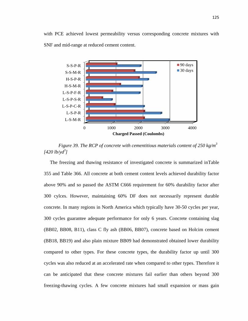
125
with PCE achieved lowest permeability versus corresponding concrete mixtures with
SNF and mid-range at reduced cement content.
Figure 39. The RCP of concrete with cementitious materials content of 250 kg/m3
[420 lb/yd3]
The freezing and thawing resistance of investigated concrete is summarized inTable
355 and Table 366. All concrete at both cement content levels achieved durability factor
above 90% and so passed the ASTM C666 requirement for 60% durability factor after
300 cylces. However, maintaining 60% DF does not necessarily represent durable
concrete. In many regions in North America which typically have 30-50 cycles per year,
300 cycles guarantee adequate performance for only 6 years. Concrete containing slag
(BB02, BB08, B11), class C fly ash (BB06, BB07), concrete based on Holcim cement
(BB18, BB19) and also plain mixture BB09 had demonstrated obtained lower durability
compared to other types. For these concrete types, the durability factor up until 300
cycles was also reduced at an accelerated rate when compared to other types. Therefore it
can be anticipated that these concrete mixtures fail earlier than others beyond 300
freezing-thawing cycles. A few concrete mixtures had small expansion or mass gain
0 1000 2000 3000 4000
L-S-M-R
L-S-P-R
L-S-P-C-R
L-S-P-S-R
L-S-P-F-R
H-S-M-R
H-S-P-R
S-S-M-R
S-S-P-R
Charged Passed (Coulombs)
90 days
30 days

126
throughout the 300 cycles. Table 35 and Table 36 report on the mass loss at 300 cycles
for all the concrete mixtures.
Figure 40. The mass loss of concrete with cementitious material content of 279 kg/m3
[470 lb/yd3] at 300 freezing-thawing cycles
-1.00 0.00 1.00 2.00 3.00 4.00 5.00
L-S-M
L-S-N
L-S-P
L-S-M-S
L-S-N-S
L-S-P-S
L-S-M-C
L-S-N-C
L-S-P-C
L-S-M-F
L-S-N-F
L-S-P-F
H-S-M
H-S-N
H-S-P
S-S-M
S-S-N
S-S-P
Mass Loss (%)

127
Figure 41. The mass loss of concrete with cementitious material content of 250 kg/m3
[420 lb/yd3] at 300 freezing-thawing cycles
As illustrated in Figures 41 and 42 two mixtures containing slag and PCE admixtures
at both cement content levels (BB17, BB27) gained about 1% mass.
The RCP behavior of developed concrete compositions with slag obtained the lowest
overall permeability which may be due to significant 50% reduction of cement compared
to the concrete with 30% fly ash replacement.
-1.00 0.00 1.00 2.00 3.00 4.00 5.00
L-S-M-R
L-S-P-R
L-S-P-C-R
L-S-P-S-R
L-S-P-F-R
H-S-M-R
H-S-P-R
S-S-M-R
S-S-P-R
Mass Loss (%)

128
5. CONCLUSIONS
Concrete mixture can be effectively designed by optimizing two essential phases i.e.
the aggregates, and cement paste. The theoretical and experimental optimization of
aggregate and cement paste was realized with extensive concrete testing. As a result of
optimization cement content was reduced by up to 35% versus current WisDOT
specifications for concrete mixtures that satisfy all other requirements.
Aggregate optimization can enhance the compressive strength by identification of the
best blend through multiple criteria. Aggregate optimization criteria used in this research
showed consistency. Multiple criteria can be used to evaluate the effect of packing
density on concrete performance. The aggregate packing alone can be used as an
effective tool to optimize the aggregate blends of concrete designed for different
applications. The continuous power curves can serve as another criterion. The coarseness
chart can assist in elaborating the level of workability of concrete and coarseness of the
blends with binary, ternary or multi-class aggregates. The chart can also be used as a tool
to tune the aggregate blends for the mixtures with various cement contents and aggregate
combinations.
The 3D packing models that are able to imitate particulate packing and to connect the
packing with particle size distribution (PSD) can provide a quick feedback and 3D
visualization of optimal blends. The realistic combined grading curves (PSD) can deliver
better packing arrangements achievable in concrete; and developed realistic gradings
have a low deviation from the power curves. Furthermore, the results of simulation can

129
be used as a reference PSD to match with the experimental blends using various
aggregates available.
The experimental results on packing degree and performance of concrete mixtures can
provide useful relationships for the selection of the best aggregate blends and evaluate the
differences between the simulation and experimental packing due to shape and packing
methods. The high density mixtures are achievable using power curves as proved by the
simulation and experimental packings. As demonstrated by experimental and simulations
the 0.35-0.45 power curves can provide a better packing versus 0.7 power curve for the
concrete mixtures with maximum aggregate size (Dmax) typical in construction industry.
In concrete with cementitious material content of less than 300 kg/m3 the aggregate
optimization may require using higher proportions of sand, up to 50% in the aggregates
blend. Due to improved grading and packing the use of intermediate aggregates is
beneficial for concrete performance. The intermediate aggregates fractions can be used in
the blends, replacing up to 30% of the coarse aggregates depending on the type of the
aggregates.
Power curves (PC) can be used as an effective tool for aggregate optimization. The
mixtures with higher fine aggregates content can be the fitted to smaller PC exponents
such as 0.35-0.45, while binary mixtures and mixtures with lower volume of fine
aggregates are closer to power 0.5-0.7 gradings. The combined packing and grading
methods enhance the optimization procedure and can be used as a tool for comparison of
various aggregate blends and mixture proportioning. Also, the use of aggregate packing

130
as a tool to optimize concrete mixtures provides a good prediction for the compressive
strength and explains the difference in concrete performance.
The compressive strength of concrete can be correlated with the packing degree of
aggregates. This correlation is more pronounced for Southern aggregates and is more
clear at the age of 7 days. As a result of aggregate optimization, the concrete compressive
strength can be increased by up to 37% (31.3 vs. 22.8 MPa for S9 and S1 mixtures based
on Southern aggregates, accordingly) and, consequently, enhanced performance can be
used to further reduce the volume of cementitious materials. The optimization of the
aggregate’s grading with ternary aggregate blends can greatly assist in this process.
However, no strength correlation was observed for Northern aggregates which may be
due to the difference in shape (round) and texture of aggregates.
The heat of hydration of the cement paste or mortar can be used for optimization of
dosage of HRWRA/WRA chemical admixtures prior to application in concrete mixtures.
The optimization of chemical admixtures is essential when various cements, SCMs, and
other chemical admixtures are used.
The optimized concrete mixtures with PCE admixtures enable up to 10 % reduction of
W/C ratio and also can provide an excellent compatibility with AE and various SCMs. As
a result of an additional strength gain due to reduced W/C ratio, the cement content can
be reduced by 12% and 35% to 279 kg/m3 [470 lb/yd
3] and 249.2 kg/m
3 [420 lb/yd
3],
respectively versus current WisDOT specification requirement.
The use of PCE admixtures and class C fly ash enables to reduce in W/C and enhance
the workability. The combination of the two materials works perfect in terms of

131
mechanical performance to achieve strength as high as 40 MPa at 28 days and above 60
MPa at 90 days.
The use of class F fly ash requires the application of PCE and adjustment of air
content that enables the reduction of W/CM ratio and resulting in a higher strength above
acceptable ranges.
The use of aggregate optimization and incorporation of additional air (by using higher
dosage of AE admixture) beyond conventional specifications may be essential in low
cement mixtures (249.2 kg/m3 [420 lb/yd
3]) are designed.
The fresh density and air content of concrete mixtures have a strong relationship and
the air content can be estimated from the fresh density-air content graph as illustrated in
Figure 31. The relationship between air content and fresh density of tested final mixtures
The modulus of rupture (MOR) obtained from the flexural center-point (3-point)
loading of the beams has a good correlation with corresponding compressive strength as
demonstrated for various mixtures and ages.
The permeability for low cement content concrete produced at the same W/CM ratio is
reduced due to the reduced volume of cementitious phase and lower permeability of
predominant aggregate fraction. However, the higher porosity in cementitious materials
associated with higher W/CM causes higher transport properties of the matrix.
Various mixtures performed differently in RCP performance, but had very similar
response in freeze-thaw tests. All investigated concrete mixtures had selectively higher
air content (achieved by application of AE admixture) and excellent freeze-thaw

132
resistance. The use of SCMs and various W/CM ratios can lead to variations and
differences in microstructure of cementitious system in different durability tests. The
differences in in air content, saturation degree, as well as volume of cement paste and
aggregates also affect the transport properties and freeze-thaw resistance.
The developed approaches and test results can serve as a solid foundation for
specification of sustainable concrete with reduced use of cementitious materials and
enhanced performance as required for WisDOT applications.

133
6. FUTURE RESEARCH
The various aspects of reported research can be further extended. A comprehensive
multi-scale model of concrete can be developed based on extensive test results of this
research; and furthermore, this model can be used for development of a new concrete mix
design procedure that targets the low cement contents minimizes the experiments, and
serves the applications for WisDOT. This procedure can involve the use of different
components of paste, mortar and concrete into consistent design routine for the mixtures
with required performance level.
The development of a software package for aggregate optimization as a tool based on
the results of packing simulations, theoretical models, and experimental approaches can
be useful for the implementation of reported research effort.

134
REFERENCES
1. Report Card for America’s Infrastructure, 2013, ASCE.
2. Van Dam, T., et al., Sustainable concrete pavements: A manual of practice. 2012.
3. Abrams, D., A tribute to Proportioning Concrete Mixtures. ACI Special
Publication, 2008. 249.
4. Abrams, D., Proportioning of concrete mixtures Structural Materials Research
Laboratory December 1918. Bulletin No.1.(Lewis Institute Chicago).
5. Gilkey, J.H., Water-Cement Ratio versus Strength – Another Look ACI Journal
Proceeding April 1961. (4): p. 57.
6. Neville, A.M., Proportioning of concrete mixtures. 1995: p. 269-272.
7. Neville, A., Properties of concrete. Fourth and final edition standards, 1996,
Pearson, Prentice Hall. ISBN 0-582-23070-5. OCLC.
8. Goltermann, P. and V. Johansen, Packing of aggregates: an alternative tool to
determine the optimal aggregate mix. ACI Materials Journal, 1997. 94(5).
9. de Larrard, F. and T. Sedran, Optimization of ultra-high-performance concrete by
the use of a packing model. Cement and Concrete Research, 1994. 24(6): p. 997-
1009.
10. Vorobiev, V., Application of physical and mathematical methods in concrete
research. Visshaya Shkola, Moscow, 1977.
11. Fuller, W.B. and S.E. Thompson, The laws of proportioning concrete.
Transactions of the American Society of Civil Engineers, 1906. 57(2): p. 67-143.
12. American Concrete Institute, Aggregates for Concrete Bulletin E1-07, First Print,
2007.
13. Sobolev, K. and A. Amirjanov, Application of genetic algorithm for modeling of
dense packing of concrete aggregates. Construction and Building Materials, 2010.
24(8): p. 1449-1455.
14. de Larrard, F., A method for proportioning high-strength concrete mixtures.
Cement, concrete and aggregates, 1990. 12(1): p. 47-52.
15. de Larrard, F. and A. Belloc, The influence of aggregate on the compressive
strength of normal and high-strength concrete. ACI Materials Journal, 1997.
94(5).
16. Hansen, T.C. Influence of aggregate and voids on modulus of elasticity of
concrete, cement mortar, and cement paste. in ACI Journal Proceedings. 1965.
ACI.
17. Li, S.-t.i. Proposed Synthesis of Gap-Graded Shrinkage-Compensating Concrete.
in ACI Journal Proceedings. 1967. ACI.
18. Richardson, D.N., Aggregate gradation optimization: literature search. 2005.
19. Sobolev, K., et al. Packing of aggregates as an approach to optimizing the
proportioning of concrete mixtures aggregates: asphalt concrete, portland cement
concrete, bases, and fines, presented at. 2004. ICAR/AFTRE/NSSGA Symp.
20. Fennis, S., Design of ecological concrete by particle packing optimization2011:
TU Delft, Delft University of Technology.
21. Roy, D., et al., Concrete components packing handbook, 1993.

135
22. Powers, T., Properties of Fresh Concrete, John Wiley and Sons. Inc., New York,
1968: p. 301.
23. Andersen P.J., J.V., Particle packing and concrete properties. Material Science of
Concrete, The American Ceramic Society, Inc., 1991(II).
24. Aim, R.B. and P. Le Goff, Effet de paroi dans les empilements désordonnés de
sphères et application à la porosité de mélanges binaires. Powder Technology,
1968. 1(5): p. 281-290.
25. Toufar, W., M. Born, and E. Klose, Beitrag zur Optimierung der Packungsdichte
polydisperser körniger Systeme. Freiberger Forschungsheft, 1976. 558(29-44): p.
201.
26. De Larrard, F., Concrete mixture proportioning: a scientific approach1999: CRC
Press.
27. Dewar, J., Computer modelling of concrete mixtures2002: CRC Press.
28. Brouwers, H. and H. Radix, Self-compacting concrete: theoretical and
experimental study. Cement and Concrete Research, 2005. 35(11): p. 2116-2136.
29. Vogt, C. Ultrafine particles to save cement and improve concrete properties. in
Nordic Concrete Research, Sandefjord, Norway, June 13-15, 2005. 2005. The
Nordic Concrete Federation.
30. Feret, R., Sur la compactie des mortiershyrdauliques, Ann.Ponts Chaussée,
mé.moires etdocuments. Série 7, 1892. no. IV: p. 5-164.
31. Fu, G. and W. Dekelbab, 3-D random packing of polydisperse particles and
concrete aggregate grading. Powder Technology, 2003. 133(1): p. 147-155.
32. Kolonko, M., S. Raschdorf, and D. Wäsch, A hierarchical approach to estimate
the space filling of particle mixtures with broad size distributions. submitted to
Powder Technology, 2008.
33. Sobolev, K. and A. Amirjanov, The development of a simulation model of the
dense packing of large particulate assemblies. Powder Technology, 2004. 141(1):
p. 155-160.
34. Yurdakul, E., et al., A paper to be submitted to Journal of Materials in Civil
Engineering (ASCE). Proportioning for performance-based concrete pavement
mixtures, 2013: p. 65.
35. Ashraf, W. and M. Noor, Performance-evaluation of concrete properties for
different combined aggregate gradation approaches. Procedia engineering, 2011.
14: p. 2627-2634.
36. Zhao, H., et al., The effect of coarse aggregate gradation on the properties of self-
compacting concrete. Materials & Design, 2012. 40: p. 109-116.
37. Moini Mohamadreza, Muzenski Scott, Ismael Flores-Vivian, Sobolev Konstantin.
‘‘Aggregate optimization for concrete mixtures with low cement factor’’, (2nd
international) conference on concrete and reinforced concrete: glace at future.
Vol. 4, Moscow, May 12, 2014, pp. 349–59. 38. Torquato, S., T.M. Truskett, and P.G. Debenedetti, Is random close packing of
spheres well defined? Physical review letters, 2000. 84(10): p. 2064.
39. Kwan, A. and C. Mora, Effects of various, shape parameters on packing of
aggregate particles. Magazine of concrete Research, 2002. 53(2): p. 91-100.
40. Stroeven, P. and M. Stroeven, Assessment of packing characteristics by computer
simulation. Cement and Concrete Research, 1999. 29(8): p. 1201-1206.

136
41. Mostofinejad, D. and M. Reisi, A new DEM-based method to predict packing
density of coarse aggregates considering their grading and shapes. Construction
and Building Materials, 2012. 35: p. 414-420.
42. Moini, M. and A. Lakizadeh, Concrete Workability: An Investigation on
Temperature effects Using Artificial Neural Networks. AuthorHouse, 2011.
43. Sobolev, K. and A. Amirjanov, A simulation model of the dense packing of
particulate materials. Advanced Powder Technology, 2004. 15(3): p. 365-376.
44. Sobolev, K., The development of a new method for the proportioning of high-
performance concrete mixtures. Cement and Concrete Composites, 2004. 26(7):
p. 901-907.
45. https://pantherfile.uwm.edu/sobolev/www/V_LAB/.
46. Moini, M. R., A. Lakizadeh, and M. Mohaqeqi. "Effect of mixture temperature on
slump flow prediction of conventional concretes using artificial neural
networks." Australian Journal of Civil Engineering 10, no. 1 (2012). 47. Collepardi, S., et al., Mechanisms of Actions of Different Superplasticizers For
High Performance Concrete. ACI Special Publication, 1999. 186.
48. Ramseyer, C.C. and R. Kiamanesh, Optimizing Concrete Mix Designs to Produce
Cost Effective Paving Mixes, 2009, Civil Engineering and Environmental Science,
University of Oklahoma.
49. Rached, M., M. De Moya, and D.W. Fowler, Utilizing aggregates characteristics
to minimize cement content in portland cement concrete. International Center for
Aggregates Research (ICAR 401), University of Texas, Austin, USA, 2009.
50. Quiroga, P.N. and D.W. Fowler, The effects of aggregates characteristics on the
performance of Portland cement concrete, 2004, International Center for
Aggregates Research, University of Texas at Austin.
51. De Larrard, F. and T. Sedran, Mixture-proportioning of high-performance
concrete. Cement and Concrete Research, 2002. 32(11): p. 1699-1704.
52. Sobolev, K. and S. Soboleva, High-Performance Concrete Mixture
Proportioning. ACI Special Publication, 1998. 179.
53. Peterson, K., L.L. Sutter, and G. Anzalone, Reduction of Minimum Required
Weight of Cementitious Materials in WisDOT Concrete Mixes, 2011.
54. Ji, T., et al., A mix proportion design method of manufactured sand concrete
based on minimum paste theory. Construction and Building Materials, 2013. 44:
p. 422-426.
55. Moini M., Flores-Vivian I., Amirjanov A., Sobolev K., The Optimization of
Aggregate Blends for Sustainable Low Cement Concrete. Construction &
Building Materials Journal, 2015.
56. Noguchi, T., I. Maruyama, and M. Kanematsu. Performance based design system
for concrete mixture with multi-optimizing genetic algorithm. in Proceedings of
the 11th International Congress on the Chemistry of Cement “Cements
Contribution to the Development in the 21st Century”, Durban. 2003.
57. Yeh, I.-C., Computer-aided design for optimum concrete mixtures. Cement and
Concrete Composites, 2007. 29(3): p. 193-202.
58. Cheng, M.-Y., D. Prayogo, and Y.-W. Wu, Novel Genetic Algorithm-Based
Evolutionary Support Vector Machine for Optimizing High-Performance
Concrete Mixture. Journal of Computing in Civil Engineering, 2013. 28(4).

137
59. Fennis, S.A. and J.C. Walraven, Using particle packing technology for
sustainable concrete mixture design. Heron, 57 (2012) 2, 2012.
60. Liu, R., et al., Optimization of cementitious material content for sustainable
concrete mixtures. Journal of Materials in Civil Engineering, 2011. 24(6): p. 745-
753.
61. Easa, S.M. and E.K. Can, Optimization model for aggregate blending. Journal of
construction engineering and management, 1985. 111(3): p. 216-230.
62. Cordon, W.A. and H.A. Gillespie. Variables in concrete aggregates and Portland
cement paste which influence the strength of concrete. in ACI Journal
Proceedings. 1963. ACI.
63. Koehler, E.P., Aggregates in self-consolidating concrete2007: ProQuest.
64. Simon, M.J., E.S. Lagergren, and K.A. Snyder. Concrete mixture optimization
using statistical mixture design methods. in Proceedings of the PCI/FHWA
international symposium on high performance concrete. 1997.
65. Kwan, A. and H. Wong, Packing density of cementitious materials: part 2—
packing and flow of OPC+ PFA+ CSF. Materials and structures, 2008. 41(4): p.
773-784.
66. Bergman, L.A. Optimization of Portland-Pozzolan Concrete, Airport Runways. in
Construction and Materials Issues 2001. 1962. ASCE.
67. Aydın, S., A ternary optimisation of mineral additives of alkali activated cement
mortars. Construction and Building Materials, 2013. 43: p. 131-138.
68. Aggregate suspension mixture proportioning method. TechNote, ACI 211.6T-14.
68.
69. Andersen, P.J. and V. Johansen, A guide to determining the optimal gradation of
concrete aggregates. Contract, 1993. 100: p. 206.
70. EUROPACK: User Manual, G. M. Idorn Consult A/S, Bredevej 2, 2830 Virum,
Denmark. Jan. 1996.
71. Mangulkar, M. and S. Jamkar, Review of Particle Packing Theories Used For
Concrete Mix Proportioning. International Journal Of Scientific & Engineering
Research, 2013. 4(5): p. 143-148.
72. Andersen, P.J., Control and Monitoring of Concrete Production: A Study of
Particle Packing and Rheology: a Thesis in Concrete Technology1990: Danish
Academy of Technical Sciences.
73. Andersen, P.J. and V. Johansen, Particle packing and concrete properties1993.
74. Joisel, A., Composition des Betons Hydrauliques, Ann. l’ITBTP,58,992-1065, .
1952.
75. Poulsen, A., Cement in seawater: report on the trials, commenced in 1896 on the
reco mmendation of the society of Scaninavian Portland cement manufacturers.
1909.
76. Furnas, C.C., Flow of gases through beds of broken solids. Vol. 300. 1929: US
Govt. print. off.
77. Westman, A.R. and H. Hugill, THE PACKING OF PARTICLES1. Journal of the
American Ceramic Society, 1930. 13(10): p. 767-779.
78. Petersen, I.F., Report on Packing Models, F. L. Schmidt & Co. 1981.
79. Toufar, W., E. Klose, and M. Born, Berechnung der packungsdichte von
korngemischen. Aufbereitung-Technik, 1977. 11: p. 603-608.

138
80. Furnas, C., Grading aggregates-I.-Mathematical relations for beds of broken
solids of maximum density. Industrial & Engineering Chemistry, 1931. 23(9): p.
1052-1058.
81. Schwanda, F., Das rechnerische Verfahren zur Bestimmung des Hohlraumes und
Zementleimanspruches von Zuschlägen und seine Bedeutung für den
Spannbetonbau. Zement und Beton, 1966. 37(8-17): p. 13.
82. Reschke, T., Der Einfluss der Granulometrie der Feinstoffe auf die
Gefügeentwicklung und die Festigkeit von Beton2001.
83. Stovall, T., F. De Larrard, and M. Buil, Linear packing density model of grain
mixtures. Powder Technology, 1986. 48(1): p. 1-12.
84. Yu, A. and N. Standish, Porosity calculations of multi-component mixtures of
spherical particles. Powder Technology, 1987. 52(3): p. 233-241.
85. Talbot, A.N. and F.E. Richart, THE STRENGTH OF CONCRETE-ITS
RELATION TO THE CEMENT, AGGREGATES AND WATER. Illinois Univ Eng
Exp Sta Bulletin, 1923.
86. KUMAR, S. and M. Santhanam, Particle packing theories and their application
in concrete mixture proportioning: A review. Indian concrete journal, 2003. 77(9):
p. 1324-1331.
87. Funk, J., D. Dinger, and J. Funk Jr, Coal Grinding and Particle Size Distribution
Studies for Coal-Water Slurries at High Solids Content. Final Report, Empire
State Electric Energy Research Corporation (ESEERCO), New York, NY, 1980.
88. Funk, J.E. and D. Dinger, Predictive process control of crowded particulate
suspensions: applied to ceramic manufacturing1994: Springer Science &
Business Media.
89. Walker, W., Persistence of Granular Structure during Compaction Processes.
Kona, 2003. 21: p. 133-142.
90. Zheng, J., P.F. Johnson, and J.S. Reed, Improved equation of the continuous
particle size distribution for dense packing. Journal of the American Ceramic
Society, 1990. 73(5): p. 1392-1398.
91. Peronius, N. and T. Sweeting, On the correlation of minimum porosity with
particle size distribution. Powder Technology, 1985. 42(2): p. 113-121.
92. Garas, V. and K. Kurtis, Assessment of methods for optimising ternary blended
concrete containing metakaolin. Magazine of concrete Research, 2008. 60(7): p.
499-510.
93. Hunger, M., An integral design concept for ecological self-compacting concrete,
2010, Technische Universiteit Eindhoven.
94. Toufar, W., M. Born, and E. Klose, Freiberger Forschungsheft A 559. VEB
Deutscher Verlag Fuer Grundstoffindustrie, 1967.
95. Zheng, J. and P. Stroeven. Computer Simulation of Particle Section Patterns from
Sieve Curves for Spherical Aggregate. in Modern concrete materials: binders,
additions and admixtures: proceedings of the international Conference held at the
University of Dundee, Scotland, UK on. 1999.
96. Snoeijer, J.H., et al., Packing geometry and statistics of force networks in
granular media. Physical Review E, 2004. 70(1): p. 011301.
97. Gram, A. and J. Silfwerbrand, Computer simulation of SCC flow. Betonwerk und
Fertigteil-Technik, 2007. 73(8).

139
98. Roussel, N., et al., Computational modeling of concrete flow: General overview.
Cement and Concrete Research, 2007. 37(9): p. 1298-1307.
99. Stroeven, P., J. Hu, and Z. Guo, Shape assessment of particles in concrete
technology: 2D image analysis and 3D stereological extrapolation. Cement and
Concrete Composites, 2009. 31(1): p. 84-91.
100. Kwan, A., C. Mora, and H. Chan, Particle shape analysis of coarse aggregate
using digital image processing. Cement and Concrete Research, 1999. 29(9): p.
1403-1410.
101. Mora, C. and A. Kwan, Sphericity, shape factor, and convexity measurement of
coarse aggregate for concrete using digital image processing. Cement and
Concrete Research, 2000. 30(3): p. 351-358.
102. Kwan, A. and W. Fung, Packing density measurement and modelling of fine
aggregate and mortar. Cement and Concrete Composites, 2009. 31(6): p. 349-
357.
103. Flores-Vivian, Ismael, R. Pradoto, Mohamadreza Moini, and Konstantin Sobolev.
"The use of nanoparticles to improve the performance of concrete." In Nano
Conference. 2013.
104. Konstantin Sobolev, Mohamadreza Moini, Steve Cramer, Ismael Flores-Vivian,
Scott Muzenski, Rani Pradoto, Ahmed Fahim, Le Pham, Marina Kozhukhova,
"Laboratory Study of Optimized Concrete Pavement Mixtures", No. 0092-13-04.
2016.
105. Shilstone Sr, J.M., Concrete mixture optimization. Concrete International, 1990.
12(6).