The Optimal Level of Progressivity in the Labor Income Tax in a

Model with Competitive Markets and Idiosyncratic Uncertainty *

Toke Ward Petersen

September 2001 Abstract In a world where labor earnings are uncertain and borrowing-constraints are present, progressive taxation is likely to have risk-mitigating benefits for consumption-smoothing agents; higher tax payments are due in periods of life when income is relatively high, and less tax must be paid when income is low. This lowers the probability that the borrowing constraint becomes binding. The question is if this income-smoothing risk-mitigating property of progressive taxation has any value to the consumers? Simulations using a large-scale computable general equilibrium model with competitive markets show that consumers prefer progressive taxation of labor earnings to proportional taxation - a result that is contrary to the findings in the deterministic framework by Auerbach and Kotlikoff (1987). However, there is a trade-off between the positive risk-migating properties of progression, and the negative distortionary effects; indeed it turns out that there is an optimal level of progressivity. JEL classification: H21, D91, E21, C68.

Keywords: idiosyncratic income uncertainty, optimal progressivity.

* Earlier versions of this paper have benefitted from comments by Larry Kotlikoff, Carlo Perroni, Shantayanan Devarajan, Lars Haagen Pedersen and Henrik Jacobsen Kleven, as well as participants at the Spring Meeting for Young Economists (SMYE) held in Copenhagen in April 2001. Thanks to Lars Haagen Pedersen for useful comments and suggestions. The usual disclaimer applies. E-mail: toke.ward.petersen@econ.ku.dk.

Table of Contents: 1. Introduction . . . . . . . . . . . . . . . . . . . . 5

2. A General Equilibrium Model . . . . . . . . . . . . . . 7

3. Calibration . . . . . . . . . . . . . . . . . . . . 16

4. Results . . . . . . . . . . . . . . . . . . . . . 23

5. Sensitivity Analysis . . . . . . . . . . . . . . . . . 33

6. Summary . . . . . . . . . . . . . . . . . . . . 38

References . . . . . . . . . . . . . . . . . . . . 41

1 Introduction

Traditional analyses of progressive taxation in competitive Computable Gen-eral Equilibrium (CGE) models, e.g. Auerbach and Kotlikoff (1987, chapter8), have concluded that progressive taxation has a negative effect on wel-fare. The reason is intuitive: in this relatively simple model the singlerepresentative agent pays a certain amount of taxes over the life-cycle, andprogressivity in the taxation of labor earnings discourages labor supply, andhence lowers welfare.1 However, it is easy to think of beneÞts from pro-gressive income taxation that are not captured in this simple framework.2

For instance progressive taxation is - in an uncertain world - likely to haverisk-mitigating beneÞts for the consumption-smoothing agents: higher taxpayments are due in periods of life when income is relatively high - andconversely less taxes must be paid when income is low. In a world withperfect capital markets this is irrelevant: the timing of tax payments (in acash-ßow sense) does not matter as long as the present value of the paymentstream is constant. In the rather realistic case that there are imperfectionsin the capital markets - for instance if the rate of return on savings is lowerthan the cost of borrowing, or if the consumer is constrained from borrowingagainst anticipated future income - this conclusion may change.

Inability to borrow against future income is particularly relevant, if the con-sumer�s future income is uncertain. For the consumer progressive taxationlowers variability in after-tax earnings compared to pre-tax earnings, andlowers the probability that the borrowing constraint becomes binding. Doesthis after-tax income smoothing property of progressive taxation have anyvalue to the consumers? On the Þrm side, one can make a similar argument,and hedging can be seen as the Þrm equivalent; for a Þrm it will generally beoptimal to hedge a volatile earnings stream, if taxes are a convex function ofearnings (Smith and Stulz, 1985). For the consumer, it may be the case thatthe positive risk-mitigating effect from progressive taxation can counteractthe negative distortionary effects? Or perhaps the risk-mitigating effect caneven outweigh the distortionary effects?

This paper attempts to answer this question in a CGE model. Overlappinggenerations of consumers face idiosyncratic uncertain labor income in each

1A similar conclusion is obtained in models with multiple agents (Altig, Auerbach,Kotlikoff, Smetters and Waliser, 2001); in addition inter-agent redistribution through tax-payments becomes an issue.

2With imperfect labor markets the standard result can reverse: progression is good.See Lockwood and Manning (1993).

5

period of their lives. The uncertainty is only present at the individual level,which means that aggregate variables are not (directly) inßuenced (i.e. thereis no aggregate uncertainty). Since borrowing is permitted, agents have toself-insure against variability in income. The government sector levies taxeson income and uses the revenue for public expenditures. The production sideis standard: Þrms produce the single good using capital and labor accordingto a constant return to scale technology.

Analyses using models with idiosyncratic earnings uncertainty and borrow-ing constraints started with the seminal papers by Aiyagari (1994, 1995)3.Subsequently the models have been used to analyze precautionary sav-ings behavior and social security issues [Hubbard and Judd (1987); Hub-bard, Skinner and Zeldes (1994, 1995); úImrohoroùglu, úImrohoroùglu and Joines(1993, 1995) ; Huggett and Ventura (1997); Huang, úImrohoroùglu and Sargent(1997)]4, effects of a ßat tax reform [Ventura (1999)], and capital incometaxation [úImrohoroùglu (1998)]. The only other paper focusing on propor-tional versus progressive taxation is Castaneda, Diaz-Gimenez and Rios-Rull(1999). However, most of these models have either been partial equilibrium,used a Ramsey formulation, or had exogenous labor supply. In contrastthis paper presents general equilibrium calculations with overlapping gen-erations of consumers with endogenous labor supply. Apart from the newfeatures (idiosyncratic uncertainty and borrowing constraints), the model iskept as close as possible to Auerbach and Kotlikoff (1987, chapter 8); yetthe added features change the model fundamentally. Firstly, the presence ofuncertainty in earnings gives the consumers a precautionary savings motive.As pointed out by Engen and Gale (1996) savings of the precautionary typeare less sensitive to the rate of return than pure life-cycle savings; thereforethe savings elasticity is likely to be lower in a situation with precautionarysavings5. Secondly, the framework makes it possible to include the positiverisk-mitigating effects from progressive taxation - these cannot be capturedby the single-agent representative framework used by Auerbach and Kot-

3Aiyagari (1994) investigates the precautionary savings effects in a Ramsey model (butis not like the present paper concerned with policy applications).

4This class of models is well suited for analysis of social security, since the models cancapture the risk-sharing properties of social security in a way that is not possible withinthe deterministic single-agent representative framework of Auerbach and Kotlikoff (1987).An overview of the analysis of social security can be found in úImrohoroùglu, úImrohoroùgluand Joines (1999).

5This effect could potentially be important: Engen and Gale (1996) report that theresponse in savings to changes in consumption taxation is 80 per cent smaller in a stochasticlife-cycle model compared to a certainty life-cycle model. This smaller savings elasticityseem to be better in accordance with empirical evidence (Deaton, 1992).

6

likoff (1987).

In the simulations two taxes are present: a capital income tax and a laborincome tax, but only the latter tax will be changed in the simulations. Theresults of the analysis turns out to be quite surprising, and challenge theconventional wisdom derived from a simple deterministic model: in fact thesimulations show that consumers ex-ante actually prefer progressive to pro-portional taxation of labor income. Hence the smoothing (or risk-mitigating)property of progressivity more than outweighs the negative effects from theincreased distortion, and it turns out that there is in fact an optimal level ofprogression. The sensitivity analysis shows that the conclusions depend onthe speciÞcation of uncertainty - the more volatile the earnings the largerthe beneÞts from progressivity.

This paper is organized as follows. Section 2 contains a description of themodel used - this includes a description of the consumers, the producers andthe government sector. Section 3 describes how the model is calibrated, aswell as the numerical solution methods employed. Section 4 presents theresults of the central case, which includes aggregate effects, life-cycle effects,as well as distributional effects. Section 5 presents a sensitivity analysis ofthe results, and Þnally section 6 summarizes the Þndings.

2 A General Equilibrium model

The model described here is a relatively standard stochastic general equilib-rium model6. To simplify matters, we will only look at the stationary stateof the model, which means that all time indices are removed in the formulaebelow.

2.1 The Consumers

The consumers in the model are almost similar to Auerbach and Kotlikoff(1987) (the �A-K model�): they live for J periods, and seek to maximizetheir life-time utility function subject to their budget constraint. Their util-ity function is additive separable, and they incur utility from consumptionand leisure. They face a borrowing constraint in every period, and as wellas (the usual) life-time budget constraint. Labor income arise from sale

6Closest related work is úImrohoroùglu, úImrohoroùglu and Joines (1995) and Huggett andVentura (1997).

7

of labor services - the income from this is uncertain, due to a stochasticproductivity term (described below). Since income in each period is un-certain, solving the consumers� problem is easier formulated as a dynamicprogramming problem, which is the way it is presented below.

2.1.1 A recursive approach

The recursive maximization problem for a representative consumer (withthe start-of-period assets aj−1 and the productivity category dj−1) is givenby:

Vj (aj−1, dj−1) = max{cj ,lj ,aj}

!1

(1−1/γ)u (cj , lj)(1−1/γ) + β

"b

πb (dj−1)Vj+1 (aj, b)

#(1)

with the budget constraint:

aj = (1 + r)aj−1 +w (1− lj) ej (dj−1)− pcj − TAX (2)

where the agent is subject to the liquidity-constraint:

aj ! 0 (∀j) (3)

the consumption-constraint:

cj ! 0 (∀j) (4)

and the leisure constraint:

1 ! lj ! 0 (∀j) (5)

where

aj is the end-of-period assets, ej (dj−1) is the productivity in period j forlabor with the start of period7 productivity dj−1, cj is the consumptionin period j, lj is the leisure enjoyed by generation j, γ is the household�sintertemporal elasticity of substitution, β is the one-period discount factor,πb (d) is the probability that next period�s labor productivity will be b given

7Rather this was their productivity at the end-of-last period, since assets and produc-tivity use end-of-period notation. Thus the productivity level dj−1 is active (earns laborincome) in period j. Therefore ej (dj−1) belong together.

8

it is d in this period8, r is the one-period interest rate, w is the wage andp is the consumer price level. TAX is taxes paid, and is the sum of aconsumption tax, an interest income tax and a labor income tax:

TAX = TAXC (pcj) + TAXA (raj−1) + TAXL ((1− lj) ej (dj−1)w) (6)

where TAXC is the consumption tax, TAXA is the taxation of interestincome, TAXL is the taxation of labor income.

Notice the dating rules used: the end-of-period convention.9 The Þrst periodfor the consumer is j = 1, which means that the consumer�s problem whenentering the economy is to solve V1(a0, d0). Since the consumers live for Jperiods, we exogenously set V56 (·) = 0.

Earnings

The labor productivity falls in one of D categories, and is age-dependentthrough the function ej (d). To simplify matters we assume that productivitycan be separated in an age- and a category effect, such that ej (d) can bewritten as the product, ej (d) = $ejed. The transition between categoriesof labor productivity is a Þrst order Markov process, with age-independenttransition probabilities π. One can think of the labor productivity, ej (d),as following a random walk with a drift (a special non-linear hump-shapeddrift), $ej, as well as the random walk component, ed.

Uncertainty in earnings is caused by variability in the labor productivity. Asformulated above the earnings uncertainty is a Þrst order Markov process,where the earnings level tomorrow only depends on earnings level today(the Markov formulation makes it possible to introduce �persistence� inproductivity - see the random walk formulation below).

Taxes

The tax-functions (TAXC , TAXA and TAXL) allow for progressive taxa-tion schemes. We use the same speciÞcation10 of the progression system as

8This implies that%

d πb (d) = 1.9Also notice the timing of information: at the time the consumer solves the problem

Vj (aj−1, dj−1), he knows the relevant productivity in the j�th period period (which isdj−1) and his assets at the beginning of the period (aj−1). In other words the uncertaintyabout productivity concerns future productivity, and not the productivity in this period.10This speciÞcation represents a simpliÞcation. It disregards the fact that most actual

tax systems are piece-wise linear tax systems, and not of the continuously increasingmarginal tax type considered here.

9

Auerbach and Kotlikoff (1987, ch. 8), and assume that the marginal taxrates take the form:

τ = τ + κB (7)

where τ is the marginal tax applicable at zero income (the �intercept�), B isthe taxable amount (the �base�), and κ is the progressivity parameter (the�slope�). If κ = 0 we have a proportional tax system. The average rate ofa system given by equation (7) is

τ = τ + κB

2(8)

This formula is applied similarly to taxation of interest income, labor incomeand consumption, and we have the tax functions:

TAXA (BA) = BAτA = BA

&τA + κA

BA2

'TAXL (BL) = BLτL = BL

&τL + κL

BL2

'TAXC (BC) = BCτC = BC

&τC + κC

BC2

'

Utility

The annual utility function is the CES-function

u (c, l) =(c(1−1/ρ) + αl(1−1/ρ)

) 1(1−1/ρ) (9)

where α is a taste parameter reßecting the joy of leisure, and ρ is an elasticityof substitution between leisure and consumption.

The consumer has two state-variables: the assets (aj) and the labor-productivity(dj), where the Þrst is a value and the second is a category, i.e. the Þrst iscontinuous and the second is discrete. Notice that assets are not allowed tobe negative at any point in time.

2.1.2 Solving the consumer�s problem

The optimization problem facing an individual is one of Þnite-state, Þnitehorizon dynamic programming11. The decision rules can be found by back-11Using the terminology in Rust (1996) we are dealing with a Discrete Time Discounted

Markov Decision Process.

10

wards recursion from the last period of life.

We start by reducing the number of control-variables by substituting thebudget constraint into the Value-function12. First we isolate cj in the budgetconstraint:

cj =(1 + r)aj−1 − aj + (1− lj) ej (dj−1)w + λ− TAX

p

and substitute this and the CES-utility-function (9) into the Value-function:

Vj (aj−1, dj−1) (10)

= max{lj ,aj}

1(1−1/γ)

&(c

(1−1/ρ)j + αl

(1−1/ρ)j

) 1(1−1/ρ)

'(1−1/γ)

+β%b πb (dj−1)Vj+1 (aj , dj)

Last period

Since death is certain beyond period J (hence V56 = 0) and there is nobequest motive in the model, the choice in period J is to consume everythingthat is left, plus whatever income is generated in that period. With a∗J = 0,we can simplify the last-period problem. Consumption is:

cJ =(1 + r) aJ−1 + (1− lj) eJ (dJ−1)w − TAX

p

and the associated utility is

VJ (aJ−1, dJ−1) = max{cJ , lJ}

!1

(1−1/γ)

&(c

(1−1/ρ)J + αl

(1−1/ρ)J

) 1(1−1/ρ)

'(1−1/γ)#(11)

We obtain the argmax for lJ (which we later will call l∗J) and for cJ (whichwe later will call c∗J) by solving equation (11) numerically.12By substituting consumption (c) away, we reduce the number of control variables to

two. We could equally well have substituted the end-of-period assets (a) away - in thiscase the consumer would explicitly choose labor and consumption (and implicitly the end-of-period assets). But as noted in chapter 12 in Judd (1998), it is convenient to havecontrol variables that are also state variables.

11

Second-last period (and forwards...)

In all periods before the last period, we calculate the optimal plan for theconsumer by numerically solving equation (10). This is done in a mannerdescribed in section 3.4.

Optimal individual policy rules

Denote the optimal consumption for a consumer with the decision problemVj (aj−1, dj−1) by c∗j (aj−1, dj−1) the optimal leisure by l∗j (aj−1, dj−1), andthe optimal end-of-period asset-holdings by a∗j (aj−1, dj−1) .13 We will referto these as the individual policy rules, and for short refer to them as c∗j , l∗jand a∗j .14

2.2 Aggregation

Finally some aggregation and equilibrium conditions for the consumer:

2.2.1 Population transition

At any point in time the agents in the economy have characteristics in the(a, d) ∈ (A,D) space (the two state variables). Let γj (a, d) denote thenumber of individuals with assets a, productivity level d and age j. Thisis a stock variable, and measured at the end of the period; in other wordsγj−1 (a, d) are alive and active in period j of their lives (remember that thereis no mortality).

Calculating how many individuals are in which group - and the transitionbetween groups - is done in the following manner:

Initial: Individuals entering the economy have no assets, buttheir distribution on productivity categories is exogenously de-termined. The probability that an agent starts in category d isηd. Thus we have that the individuals active in the Þrst period

13Consider the optimal choice of assets for an individual that has been active for 1period. His optimal end-of-period-one assets are denoted a∗1 (a0, d0), - since we know thathe entered the economy with zero assets it will in fact be a∗1 (0, d0) .14 If we think of these as functions we have a∗ : A × D → A, c∗ : A × D → R+ and

l∗ : A×D → R+, where A is asset holdings, and D is productivity levels.

12

are:γ0 (0, d) = ηd (12)

Transition: In the second period individuals can have positiveassets in addition to a productivity category. A complicatingmatter is that the transition in the system is endogenously de-termined by the consumer�s choice of control variable. Thus, forj = 1, 2, ..N − 1 we have:

γj ($a, b) ="d∈D

πb (d). /0 1"a∈A

γj−1 (a, d) χ2a∗j (a, d) = $a3. /0 1 (13)

where the Þrst term is the (exogenous) transition probabilityfrom any productivity category to category b, and the secondterm is the number of individuals in the previous period whochose to their next-period assets to equal a∗j where χ (�) is anindicator function (that assumes 1 if true, and 0 if false, the con-dition being whether individuals choose the end-of-period assetswe are considering: �a). Thus we sum over all individuals that(choose) to transit to the state γj(a, b).

Terminal: At the Þnal period, the equation above reduces to:

γJ (a, b) = 0 (14)

2.2.2 Aggregate factor supply

The next aggregation issue is the aggregate labor-supply. The total labor-supply in efficiency units is given by:

L =J"j=1

"a∈A

"d∈D

γj−1 (a, d)41− l∗j (a, d)

5ej(d) (15)

The aggregate savings can be calculated in a similar fashion. The capitalstock active in period n is denoted Kn−1, so we have:

K−1 =J"j=1

"a∈A

"d∈D

γj−1 (a, d) a∗j (a, d) (16)

13

Notice that (without loss of generality) it is assumed that physical capitaldoes not depreciate.

2.3 The producers

The production side is identical to Auerbach and Kotlikoff (1987). There isa single good, that is produced using capital and labor subject to a constant-returns-to-scale technology. Labor across ages and productivity categoriesdiffer in efficiency, and we calculate the total labor supply by individualsusing equation (15) and the size of the aggregate capital stock using equa-tion (16). For the labor supply this implies that labor across productivitycategories are perfect substitutes; what matters is how many efficiency unitsare supplied.

Production takes place using a CES production function:

Y (K,L) = Λ(+K(1−1/σ) + (1− +)L(1−1/σ)

)1/(1−1/σ)(17)

where K and L are capital and labor in the period, Y is output, Λ is ascaling constant, + is a capital-intensity parameter and σ is the elasticity ofsubstitution between K and L.

2.3.1 Factor demand

With no depreciation of capital, we have the standard result that the grosswages must equal the marginal revenue product of labor (measured in effi-ciency units):

w = (1− +) Λ(+K(1−1/σ) + (1− +)L(1−1/σ)

)1/(1−1/σ)L−1/σ (18)

and the interest rate equals the marginal revenue product of capital:

r = +Λ(+K(1−1/σ) + (1− +)L(1−1/σ)

)1/(1−1/σ)K−1/σ (19)

Notice that the output price is numeraire: p = 1.

14

2.4 The government sector

The government sector is kept very simple. Government revenue is raisedby taxation of labor income, interest income and a consumption tax:

REV_TAX =J"j=1

"a∈A

"d∈D

γj−1 (a, d) TAXL241− l∗j (a, d)

5ej (dj−1)w

3+

J"j=1

"a∈A

"d∈D

γj−1 (a, d) TAXA4a∗j (a, d) r

5+

J"j=1

"a∈A

"d∈D

γj−1 (a, d) TAXC2pc∗j (a, d)

3where j is an index over generations, d an index of the labor productivitycategories, and γj (a, d) is the share of individuals in generation j with assetsa and productivity d.

The revenue from taxation is not transferred back to the consumers, but isconsumed (similarly to Auerbach and Kotlikoff (1987)).

2.5 Equilibrium

Finally we need to deÞne what we understand what is understood by anequilibrium in the model:

DeÞnition 1 A stationary equilibrium for a given set of policy arrange-ments {κa,τa, κc,τ c, κl,τ l} (progressivity and tax level) is a collection ofvalue functions Vj (a, d), individual policy rules l∗j , c

∗j and a

∗j , age-dependent

measures of agent types γj (a, d) , relative prices of labor and capital {w, r}such that

(a) the relative prices {w, r} solve the Þrm�s maximization prob-lem (satisfy equation (18) and (19))

(b) given the relative prices {w, r} and government policies {κa,τa,κc,τ c, κl,τ l} the individual policy rules l∗j , c∗j and a∗j solve theconsumer�s problem (10)

(c) individual and aggregate behavior are consistent, i.e. that Kand L satisÞes equations (15) and (16)

15

(d) the population follows the law of motion given by equations(12), (13) and (14)

(e) commodity markets clear, i.e. that production - given byequation (17) - equals consumption:

Y (K,L) =J"j=1

"a∈A

"d∈B

γj−1 (a, d) c∗j (a, d) (20)

3 Calibration

This section describes how the model is calibrated, and how the stationarystate is calculated.

3.1 The Consumer side

For the household�s intertemporal elasticity of substitution, γ, weuse the estimate used in Auerbach and Kotlikoff (1987) and set γ = 0.25.

For the one-period discount factor, β, we again use Auerbach and Kot-likoff (1987). They use a rate of time preference of 0.015, which is equivalentto β = 1

1.015 ú=0.98522.

For the taste parameter reßecting the joy of leisure, α, we use Auer-bach and Kotlikoff�s value of α = 1.5.

The elasticity of substitution between leisure and consumption, ρ,is set to 0.8 (same values as in Auerbach and Kotlikoff (1987)).

3.1.1 The age-dependent (deterministic) productivity term

As mentioned previously ej (dj−1) is separated in the two terms $ej and ed. $ejis the (deterministic) age-dependent part and here we use the same equationfor productivity over the life-cycle as Auerbach and Kotlikoff (1987), whichin turn originate from a cross-sectional regression study by Welch (1979).This hump-shaped proÞle gives an earnings proÞle that peaks at age 30,(corresponding to an actual age of 50) at wages that are 45 percent higherthan at age 1 (corresponding to 21 years). This hourly productivity proÞleover the life-cycle is illustrated in the Þgure below:

16

0,0

0,2

0,4

0,6

0,8

1,0

1,2

1,4

1,6

1 11 21 31 41 51

Figure 1. Deterministic age-dependent productivity term, $ej .An agent�s total productivity, ej (dj−1), is uncertain, and varies around thishump-shaped trend due to the stochastic term, ed. The stochastic part, ed,is modelled as a random walk, and each year the consumer�s ed-term goeseither up or down (or stays the same). Even with a relatively low probabilityfor a change in wages, of say 10 percent from one year to the next, this canamount to large differences between agents with the lowest, and the agentswith the highest productivities (i.e. high variance) over the life cycle. Agentsare relatively similar when young (low variance), but a small annual spreadin productivity can - after 55 years on the labor market - add up to largedifferences between agents.

For the ed productivity term we use a random walk on a logarithmic scale15,where each productivity category is associated with a 10 percent higher pro-ductivity compared to the previous category. In total there are 49 categorieswhere the middle category (number 24) has a unity productivity index, thecategory above has a productivity index of 1.11, the category below has aproductivity index of 1.1−1 (= 0.909), and so forth16. The lowest and high-est productivity categories are therefore respectively 1.1−24 (= 0.102) and15This is the discrete time equivalent of a geometric Brownian motion.16Notice that the Þrst category is called 0 - this is done since the Þrst index C++

vectors per deÞnition is 0 (and not 1 as usual in mathematics). Thus categories where theproductivity term ed is below unity are 0-23, and categories where ed is above unity are25-48. Thus category 24 is status quo, and e24 = 1. In general the productivity categoryof the d�th category is = (1.1)d−24. In the sensivivity analysis experiments are carried outwhere the base number is 1.05 and 1.15 instead of 1.10.

17

1.124 (= 9. 849), which is quite a wide range. However, either extreme issomething that only a very small fraction of the agents will ever experience,and most agents� productivities will ßuctuate around the hump-shaped trendshown in Figure 1.

3.1.2 SpeciÞcation of uncertainty: the Markov process

For theMarkov transition probabilities πb (d) we model the productiv-ity process as a random walk with no drift.

0

-2.25 -1.5 -0.75 0 0.75 1.5 2.25

0

Figure 2. Discrete approximation to the Normal distribution.

This is modelled as Markov chain with 7 possibilities of transition in eachperiod (this discrete approximation to the Normal distribution is illustratedin Figure 2). This means it is only possible to move ±3 states in eachdirection (plus the possibility of remaining in the same productivity categoryfrom one period to the next). The number of states represents, as pointedout by Deaton (1992, page 185), a trade-off between making a reasonablediscrete approximation to the Normal distribution and at the same time notintroducing too many states, since this causes a quadratic increase in thecomputational burden. The table below shows the 7 states, as well as theirassociated transition probabilities, and their impact on productivity:

18

transition -3 -2 -1 0 +1 +2 +3std dev -2.25 -1.50 -0.75 0 +0.75 +1.50 +2.25probability 0.0109 0.0545 0.1598 0.5467 0.1598 0.0545 0.0109∆pr�tivity (ed) -24.9% -17.4% -9.1% unch. +10% +21% +33.1%

Table 1. Transition probabilities in the Markov process.

As mentioned each of the nodes are ±10% apart measured in productivityterms. This number is in the same neighborhood as the value used in Huggett(1996), although smaller (this somewhat ad hoc speciÞcation makes thisvalue a good candidate for later sensitivity analysis). An individual whofrom one period to the next moves 2 steps up the �productivity ladder� has1.1x1.1=1.21 times (21 percent) higher productivity in next period (and theassociated probability that he moves �two steps� up is 5.45 percent). Thechanges in productivity happens from one year to the next, and with this inmind the numbers in the table above do not seem unreasonable. But evenwith these small annual changes in productivity, the fact that the consumerslive 55 periods means that there over time will be large differences betweenthe least productive and the most productive agents. This results in adistribution of productivities for the population, that over time will becomeLog Normal as illustrated in the Figure 3 below. The Þgure shows thedistribution of productivities for agents that have lived 55 periods (where thevariance in the distribution of productivities within the generation peaks).

0

0,01

0,02

0,03

0,04

0,05

0,06

0 1 2 3 4 5 6 7 8 9 10productivity

freq

uenc

y

Figure 3. Distribution of productivities for the oldest agents in thepopulation.

In order to keep the number of states low, the Markov chain is boundedbelow and above to 24 states on each side of the central node. This means

19

that the transition probability matrix is a 49x49 band diagonal matrix wherethis period�s state only can communicate with next period�s ±3 neighboringstates - a total of 7 states (the 49 states is quite a large number - it canbe compared to the 18 states in Huggett (1996)). This 49-state Markovtransition matrix is illustrated in Figure 4 on the next page.

Productivity next period

High productivity

Central node

Low productivity

Figure 4. The Markov transition matrix.

In the Þgure the light grey Þelds indicate the states to which transition ispossible from the present state (given by the row). Status quo, i.e. the indi-vidual�s productivity term ed does not change from one period to the next,is illustrated by dark grey (but note that the individual�s total productivity,ej , is likely to change from one year to the next because of the age-dependentterm: $ej ). The probability that this happens is shown in Table 1 above andis 54.67%. The probability that the individual�s productivity goes either one�step� up or down is 15.98%. Notice that it is not possible to move fromcategory 24 (the central node) to category 40 from one year to the next - itis only possible to transit ±3 steps in each direction.

20

Bounding the stochastic process above and below17 introduces a small trun-cation error since some agents (although not many) will eventually reach ei-ther the upper or lower boundary (where the probabilities must be adjustedto make each row sum to unity18 - since no agents can leave the system).Individuals that for instance �draw� a +3 productivity increase in 9 periodsin a row, will reach the upper productivity boundary (with the associatedproductivity level that is almost 10 times larger than initially, and similarlysome very unlucky individuals will reach the lower bound that is around one10th of their initial productivity. However the number of agents that reachthe upper or lower bound are 0.13 percent of all agents in the Þnal periodof their lives19, and this is a sufficiently small fraction that (given the othersources of error that are present in these computations) it is reasonably safeto assume that this truncation does not introduce any signiÞcant errors onthe results.

3.1.3 Initial distribution of productivities

The initial distribution on productivity categories is centered around thecentral node such that 54.67 percent have the productivity level 1.000 (node24), 15.98 percent have the productivity associated with nodes 25 and 23,5.45 percent have the productivity associated with nodes 26 and 22, andÞnally 1.09 percent begin with productivity levels associated with nodes 27and 21. In other words η24 = 0.5467, η23 = η25 = 0.1598, η22 = η26 =0.0545, and η21 = η27 = 0.0109.

Of cause other choices of initial distribution could be made. However theunderlying idea that individuals� productivity varies over the life cycle, fromless variability when young to span a larger spectrum later in life, seems quiteplausible.

3.2 The producers

Since the production side is identical to Auerbach and Kotlikoff and we usethe same parameters as them. The elasticity of substitution σ = 1.0, i.e.17 In this case the upper and lower bounds are 1.124 (= 9. 849) and 1.1−24 (= 0.102) .18This is done by adding the residual probability mass at the boundary value (state 0

and 48). This implies that agents who reach the upper (lower) boundary do not get stuck,but can experience a decrease (increase) in productivity the next period.19This number is found by introducing an absorbing state at the upper and the lower

bound and computing the number of agents that end up in these states after 55 periods.

21

a Cobb-Douglas production function, the capital intensity parameter, +, is0.25, and the production function constant: Λ = 0.8927.

3.3 The public sector

The initial tax is a 15 percent income tax. In all subsequent experimentsis the government revenue held constant at this level (in the literature thisis known as differential incidence experiments). Clearly the size of the gov-ernment sector is important, and is subject to sensitivity analysis in section5.2.

3.4 Solving the model in Steady State

The model is solved in a manner similar to Auerbach and Kotlikoff (1987)or úImrohoroùglu, úImrohoroùglu and Joines (1993). This means performing thefollowing procedure until convergence:

1. Guess aggregate L and K (and tax rates if they are endogenous)

2. Use the factor-demand equations ((18) and (19)) to calculate guessesfor w and r.

3. Solve the Dynamic Program and obtain the decision rules c∗j , a∗j and

l∗j .

4. Compute the new aggregate capital stock (using equation 16) and thenew labor-supply (using equation 15) (and the tax revenue if it isendogenous).

5. Check if K and L are converging - if not go to step 1, and use a convexcombination of the old and the new estimates for K and L as initialguesses (with endogenous tax rates, adjust the tax rates up(down) ifthe revenue is too low (high)).

3.4.1 Solving the dynamic program

The general equilibrium model is solved in stationary state using the it-erative techniques discussed in Auerbach and Kotlikoff (1987). The con-sumer�s problem is solved using dynamic programming as described in Pe-tersen (2001), as well as in Bertsekas (1995) and Ljungqvist and Sargent

22

(2000). Several of the techniques discussed in úImrohoroùglu, úImrohoroùgluand Joines (1998) and Judd (1998) are used to speed up the computations.

The discrete grid for assets is successively reÞned in each iteration, and whenconvergence is achieved the grid-points in the mesh are 0.0005 units apartwhich corresponds to 0.02 percent of the average asset holdings. The laborsupply is also constrained to lie on a discrete grid: in this case the grid-points are 0.00005 units apart corresponding to 0.015 percent of the averagelabor supply. ReÞning these grids further does not alter the results sig-niÞcantly but inßuences the computation time dramatically. The practicalcomputations are carried out in MS Visual C++ 5.0.

4 Results

This section presents the main results from the comparison between progres-sive and proportional labor income taxation. Before looking at the results inthe present model with idiosyncratic earnings uncertainty, it is worthwhileto review the main Þndings in chapter 8 in Auerbach and Kotlikoff (1987)who perform a similar comparison in a deterministic framework:

� Progressive taxation induces intertemporal speculation in labor supply.With progressive taxation the marginal taxes are higher in the highlyproductive years in the life-cycle. To avoid these high marginal taxes,agents choose to work less in the middle ages, and more when old.

� Removing progressivity causes a welfare increase in the new steady-state of 0.69%. This amount is sensitive to the revenue-requirements:with an approx. 66% higher revenue requirement, the gain in welfareis 1.62%.

� There is an increase in labor supply of 3.9%, an increase in the capitalstock of 5.1%, and an increase in production of 4.5%. With a higherrevenue requirement the corresponding numbers are 6.3%, 10.7% anda 7.0%.

4.1 Aggregate results

As mentioned previously experiments in this paper are of a differential inci-dence kind, i.e. that the government revenue is constant (at the level that a

23

15 percent income tax generates under a proportional income tax). In theexperiments reported below it means that the progression, κ, is increased(decreased) at the same time as the intercept, τ , is decreased (increased) (seeequation (8)). The progression of labor earnings, κ, is exogenously chosenwhile the intercept (of labor earnings), τ , is endogenously computed suchthat the overall revenue is constant.20 Notice that the capital income tax inall cases below stays at a 15 percent proportional rate.21

Progressivity κ=0 κ=0.125 κ=0.250 κ=0.375 κ=0.500 κ=0.625Production 26.832 26.648 26.489 26.345 26.219 26.104Capital stock 120.637 119.181 117.940 116.838 115.895 115.029Consumption 21.650 21.485 21.340 21.211 21.095 20.989L suppl (eff) 18.915 18.818 18.733 18.656 18.588 18.525L suppl (hours) 14.444 14.388 14.340 14.297 14.258 14.223Avg. Lsuppl eff 1.3096 1.3079 1.3064 1.3049 1.3036 1.3024L-inc tax (%) 15.000 13.977 13.106 12.354 11.697 11.117Avg. Linc tax % 15.000 15.134 15.253 15.360 15.458 15.550Util (×10−6) -5.4200 -5.4144 -5.4111 -5.4095 -5.4091 -5.4098

Table 2. Labor income tax reform.

The next table contains the same values in index (where the proportionalcase, κ = 0, is 100). Compared to the results from the deterministic model- the �Auerbach and Kotlikoff case� - we see an expected negative impactfrom progressivity on production, consumption and the capital stock. Laborsupply also goes down, and compared to the case with proportional taxation(κ = 0) the decrease in the number of efficiency units is larger than thedecrease in number of hours worked under progressive taxation. This meansthat the average efficiency per hour worked (the row labelled Avg. L-supplyeff. in the tables above) decreases with progressivity. This is the sameintertemporal labor supply effect found by Auerbach and Kotlikoff: to avoidthe high progressive taxes agents choose to work less when highly productive(middle aged), and work more when less productive (young or old). This20Auerbach and Kotlikoff (1987) chose to endogenize κ, which is the other way around.

Both methods give the same results, but for the purpose of the simulations in this paper,it is convenient to be able to Þx the level of progression exogenously.21 Ideally the optimal progressivity should be determined jointly for both available tax

instruments. However, this would add a (computationally challenging) dimension to theproblem: from a one dimensional search (for the optimal level of progression in the laborearnings), to a two dimensional search with respect to the optimal level of progression inlabor earnings and the optimal level of progression of capital earnings. The run-time ofthe present calculations makes this practically infeasible.

24

in turn affects savings: agents who retire later will tend to accumulate lessassets at a given age, than would an agent who plan to retire earlier.

Progressivity κ=0 κ=0.125 κ=0.250 κ=0.375 κ=0.500 κ=0.625Production 100 99.31 98.72 98.19 97.72 97.29Capital stock 100 98.79 97.76 96.85 96.07 95.35Consumption 100 99.24 98.57 97.97 97.44 96.95L suppl (eff) 100 99.49 99.04 99.63 98.27 97.94L suppl (hours) 100 99.61 99.28 99.98 98.71 98.47Avg. Lsuppl eff 100 99.85 99.74 99.63 99.53 99.44L-inc tax (%) 100 93.18 87.37 82.36 77.98 74.11Avg. Linc tax % 100 100.89 101.69 102.40 103.05 103.67Util 100 100.105 100.165 100.192 100.202 100.189

Table 3. Labor income tax reform (index : proportional=100).

But whereas these negative effects were captured by Auerbach and Kotlikoff,the present model also captures the positive risk-mitigating effects fromprogressive taxation. This after-tax smoothing property of the progressivetax system has value for the consumers, as can be seen from the row, Utilitynewborn, in the table: ex ante expected utility for an newborn22 is actuallylarger under the progressive scheme. This overall result stands in contrastwith the deterministic case: the average agent, embodied by a newbornconsumer, actually prefers progressive taxation. However, there is a limit tothis preference for progressivity: at some level of progressivity the negativedistortionary effects from increased taxation is larger than the positive after-tax income smoothing effects, and the overall effect will fall and eventuallybecome negative. That such an optimal level in fact exists can be seenfrom the table: for the values of κ shown in the table, the highest utilityis achieved when κ=0.5. Where exactly the optimal level of progressivity islocated cannot be determined precisely from the selected values of κ above:but it appears to be located somewhere in the interval κ ∈ [0.375, 0.625].

4.1.1 Optimal progressivity

In principle the location of the optimal level of progression can be determinedusing the model: the level of progression could be made endogenous and the22By newborn is meant an individual who has no history, i.e. does not yet know to

what productivity category he initally is assigned. Formally it is calculated as Unewborn =%j ηjV1 (0, j) where ηj is the initial distribution when the Þrst period begins.

25

expected utility of a newborn could be maximized (instead of maximizingutilities for each of the 7 initial groups of consumers given by ηi). However,more interesting than the exact optimal level given the speciÞcations usedhere, is how the welfare varies with the degree of progressivity, κ. Figure5 below shows the welfare improvement (relative to the proportional case,κ = 0) of progressive taxation for values of κ in the [0, 1] range:

0,000%

0,050%

0,100%

0,150%

0,200%

0,250%

0,0 0,1 0,2 0,3 0,4 0,5 0,6 0,7 0,8 0,9 1,0

Progression

Wel

fare

gain

Figure 5. Welfare gains from progressivity.

The Þgure shows the beneÞts from progressivity, and at some level (the op-timal level of progression, κ = 0.46875 in the Þgure) the welfare gain is thehighest. For higher levels of progressivity the welfare gain decreases (butstill remains positive). Notice that the Þgure is not symmetric: welfare goesup relatively fast for low levels of progression, whereas it decreases relativelymore slowly for levels of progression higher than the optimal level. Secondlyit should be noted that the welfare gains in all cases are positive (for theinterval under consideration). There are two effects working in oppositedirections: the beneÞcial income-smoothing effect (increasing in κ) and thenegative distortionary effect from progression for a constant revenue require-ment (increasing in κ). In addition there is an effect from the size of therevenue that must be raised (since higher revenue means higher distortions);in the Þgure this effect is kept constant, since the revenue collected in allcases is the same. In the sensitivity analysis experiments are carried out witha higher revenue requirement, which gives a different relationship betweenprogressivity and welfare gains.

26

4.2 Life-cycle behavior

The results reported in the tables above were on the aggregate level. How-ever, it is also interesting to take a look at the underlying life-cycle effects.Let us Þrst look at what happened on average for each age-group. The Þgurebelow shows the average end-of-period assets (a∗j) per generation:

0

1

2

3

4

5

6

1 6 11 16 21 26 31 36 41 46 51

Progressive

Proportional

Figure 6. Average wealth over the life cycle.

In the Þgure above, and the following Þgures, progressive will be taken tomean the previously found optimal level of progression, i.e. κ = 0.46875.The results clearly show that the decrease in wealth from Table 3 is distrib-uted evenly over the life-cycle: for every age is the average asset holdingslarger under proportional labor income taxation. This effect was largelyexpected, and can be explained by the intertemporal speculation in laborsupply that the next Þgure shows.

The results shown in this Þgure are in accordance with Auerbach and Kot-likoff (1987): under a progressive labor income tax individuals choose towork less when highly productive (middle aged), and more when less pro-ductive (i.e. old). Here the switch occurs after 38 years in the labor market(corresponding to a real age of 58): under progressive taxation individualsyounger than 58, work less hours than they would under proportional tax-ation, and reversely individuals older than 58 years work more hours underprogressive taxation. Thus there are two effects that have negative inßuenceof savings: a) there is less income to save out of when younger, and b) thereis a smaller need for a large nest-egg when old, since labor supply is higher.

27

0,00

0,10

0,20

0,30

0,40

0,50

1 6 11 16 21 26 31 36 41 46 51

Progressive

Proportional

Figure 7. Average labor supply in hours over the life cycle.

Finally Figure 8 shows what happens to consumption over the life-cycle:

0

0,1

0,2

0,3

0,4

0,5

0,6

0,7

1 6 11 16 21 26 31 36 41 46 51

Progressive

Proportional

Figure 8. Average consumption over the life cycle.

Since life-cycle income is lower under progressive taxation so is the con-sumption. Notice that consumption is not smooth: the consumer�s Keynes-Ramsey rule says to smooth annual utility, u (c, l), from equation (9) and notconsumption alone. Therefore the kink in consumption around retirementis in accordance with consumption smoothing: since the consumer cannotdecrease labor supply further, he starts purchasing more consumption goodsto smooth the annual utility.

4.3 Distributional effects

The life-cycle Þgures above showed what happened with the average agent.However behind these averages are large distributional effects. Since these

28

effects are not present in a deterministic model such as Auerbach and Kot-likoff (1987) these are of particular interest.

Figure 9 below shows how wealth is distributed in the case with proportionaltaxation. The discs in the Þgure represent the size of the population (i.e. thenumber of people) with the given age and assets - this is a way of showing3-dimensional data. The full line in Figure 6 represented an average overthese values.

0

2

4

6

8

10

12

0 5 10 15 20 25 30 35 40 45 50 55

Figure 9. Wealth distribution under proportional taxation.

Recall that current productivity in the Þrst period can be in one of 7 cate-gories, with the majority starting with a productivity level of unity (54.67%start in category 24: η24 = 0.5467). This group is represented by the largestdisc in the Þgure, since this group chooses end-of-period assets a∗1 = 0.1037.This particular group is then next period split into 7 smaller groups (ac-cording to the transition probabilities shown in Table 1). Another way ofshowing this distribution is the Þgure below that shows selected percentilesin the distribution of assets:

29

0

1

2

3

4

5

6

7

8

9

10

11

1 11 21 31 41 51

Figure 10a. Percentiles in the wealth distribution under proportionaltaxation.

In the Þgure the median (the 50th percentile) is shown with the bold line,and each of the other full lines represent the 10 percent percentiles (fromthe bottom, the 10th, 20th, 30th, 40th percentile, and above the medianthe 60th, 70th, 80th and 90th percentiles), in addition to the 2 and 98 per-centile that is represented by a dotted line. This Þgure should be comparedwith Figure 10b that shows a similar Þgure under progressive labor incometaxation.

Notice how a move to progressive labor income taxation (not surprisingly)compresses the wealth distribution: the second percentile moves marginallyup under progressivity, and the 98�th percentile goes down with around 10percent. For the richest of the rich - a very small group not shown in theÞgure - the effect is even more dramatic: the richest agent in the economymoves from a peak wealth of around 45 to 28. Similarly there are agentswith zero assets in both cases, but they are very few.

The model can also be used to show aggregate distributional effects. Figure11 below shows a Lorenz-curve of the pre-tax income. The horizontal axisshows the total population, and the vertical axis shows the total pre-taxincome.

30

0

1

2

3

4

5

6

7

8

9

10

11

1 11 21 31 41 51

Figure 10b. Percentiles in the wealth distribution under progressivetaxation.

0

10

20

30

40

50

60

70

80

90

100

0 10 20 30 40 50 60 70 80 90 100

Proportional

Progressive

Figure 11: Lorenz curve for pre-tax income.

As expected the Þgure shows that the pre-tax income distribution becomesmore even under progressive taxation of labor earnings; this is because in-dividuals with high productivity, ej (d), lower their labor supply (and vice-

31

versa for individuals with lower productivity). This effect can also be seenfrom Figure 12 below, that shows what happens to pre-tax and post-taxincome under proportional and progressive labor income taxation:

0

1

2

3

4

5

6

0 0,2 0,4 0,6 0,8 1 1,2 1,4 1,6 1,8

Proportional

Progressive

0

1

2

3

4

5

6

0 0,5 1 1,5 2 2,5

Proportional

Progressive

Figure 12. Distribution of labor earnings before taxes (left) and aftertaxes (right).

In the Þgures the earnings are along the horizontal axis, and the frequencyalong the vertical axis. The change in tax regime affects both before andafter tax earnings. For the part of the population with an income below0.6 their before-tax income is higher under progressive taxation - this effectis due to an increase in the number of hours worked. For the part of thepopulation with a higher income (around 23% of the population) the effectis the other way around: they choose to work less, and therefore receivea lower before-tax income. As can be seen from the right Þgure (showingthe after-tax earnings) the progressive tax system magniÞes this effect: thedistribution of after-tax labor earnings moves quite a lot.

Clearly the overall wealth distribution is also affected, and Figure 13 belowshows the Lorenz-curves for asset-holdings. Again this change in the Lorenz-curve does not look like much, but the fact is that it takes very large changesin the distribution to make the Lorenz-curve move substantially (this istrue for any Lorenz-curve). There are large changes going on in the wealthdistribution, which was well illustrated by the Figures 10a and 10b above.

32

0

10

20

30

40

50

60

70

80

90

100

0 10 20 30 40 50 60 70 80 90 100

Proportional

Progressive

Figure 13: Lorenz curve for assets.

5 Sensitivity analysis

This section examines the sensitivity of the results with respect to centralparameter values and speciÞcations. As with any other sensitivity analysis inCGE models, this sensitivity analysis can never be complete and exhaustive.It is impossible to try every combination of parameters and assumptions; itis necessary to restrict the attention to a smaller subset of assumptions.

Compared to Auerbach and Kotlikoff (1987) the main change in the set-upused above was the introduction of uncertainty in earnings. For this reasonit is important to examine the result�s dependence on the (somewhat ad-hoc) speciÞcation of uncertainty. The Þrst part of the sensitivity analysislooks at different speciÞcations of uncertainty. The second objection tothe A-K framework is that the public sector is too small, and that the15 percent initial income tax is too low (at least with a European contextin mind). Therefore the second sensitivity experiment is to increase therevenue requirement to 25 percent - a similar experiment is carried out inAuerbach and Kotlikoff (1987). The third interesting experiment, is to see

33

how different values of the important elasticities of substitution affect theresults - again this type of experiment is also carried out in Auerbach andKotlikoff (1987)

5.1 Alternative speciÞcations of uncertainty

As mentioned above it is not possible to make an exhaustive examinationof how the speciÞcation of uncertainty affects the results. Uncertainty wasmodelled as a random walk, and one may argue that some alternative spec-iÞcation is better. For instance earnings could be a mean-reverting process,and hence should be modelled as a so-called Ornstein-Uhlenbeck process,as in Huggett (1996). On the other hand one could argue, that produc-tivity should be modelled as a jump-diffusion process, or by some otherIto-process.23 Ultimately this choice between alternative formulations is anempirical matter. That is: which of the speciÞcations Þts the data best..

Since the purpose of this paper is to examine how uncertainty in earningsaffect policy conclusions, and not to achieve the maximum degree of re-alism per se, these alternative speciÞcations of the stochastic process willnot be pursued here. Instead it will be examined how more or less vari-ance/volatility in the random walk (i.e. more or less uncertainty) affects theresults. Previously the steps on the discrete �productivity-ladder�, ed, were10 percent apart: the section below presents the results from the policy ex-periments when the steps on the �productivity�-ladder are lower (5 percent)and higher (15 percent).

Lower volatility in productivity

With less variability/uncertainty in earnings, the model becomes closer tothe A-K model. In fact lowering the productivity stepsize to zero meansthat the model turns into the A-K model (this would make the model de-terministic). Setting the steps on the �productivity-ladder� 5 percent apart(as opposed to 10 percent in the base case), means that income is a lot lessvariable/volatile. This implies that the lowest productivity category has theproductivity index 0.31 (=1.05−24) and the highest category has the index3.23 (=1.0524) - a much smaller interval than before, where the lower andupper indices were 0.1 and 9.8 (factor 10 versus the base case�s factor 97).24

23For an introduction to these stochastic processes see Dixit and Pindyck (1994, ch. 3).24Here factor is used to mean the ratio between the highest and the lowest productivity

categories (i.e. e48/e0).

34

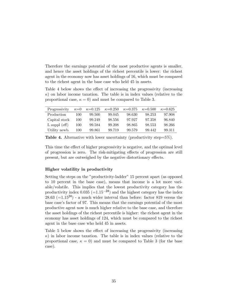
Therefore the earnings potential of the most productive agents is smaller,and hence the asset holdings of the richest percentile is lower: the richestagent in the economy now has asset holdings of 16, which must be comparedto the richest agent in the base case who held 45 in assets.

Table 4 below shows the effect of increasing the progressivity (increasingκ) on labor income taxation. The table is in index values (relative to theproportional case, κ = 0) and must be compared to Table 3.

Progressivity κ=0 κ=0.125 κ=0.250 κ=0.375 κ=0.500 κ=0.625Production 100 99.500 99.045 98.630 98.253 97.908Capital stock 100 99.249 98.556 97.927 97.358 96.840L suppl (eff) 100 99.584 99.208 98.865 98.553 98.266Utility newb. 100 99.861 99.719 99.579 99.442 99.311

Table 4. Alternative with lower uncertainty (productivity step=5%).

This time the effect of higher progressivity is negative, and the optimal levelof progression is zero. The risk-mitigating effects of progression are stillpresent, but are outweighed by the negative distortionary effects.

Higher volatility in productivity

Setting the steps on the �productivity-ladder� 15 percent apart (as opposedto 10 percent in the base case), means that income is a lot more vari-able/volatile. This implies that the lowest productivity category has theproductivity index 0.035 (=1.15−24) and the highest category has the index28.63 (=1.1524) - a much wider interval than before: factor 819 versus thebase case�s factor of 97. This means that the earnings potential of the mostproductive agent now is much higher relative to the base case, and thereforethe asset holdings of the richest percentile is higher: the richest agent in theeconomy has asset holdings of 124, which must be compared to the richestagent in the base case who held 45 in assets.

Table 5 below shows the effect of increasing the progressivity (increasingκ) in labor income taxation. The table is in index values (relative to theproportional case, κ = 0) and must be compared to Table 3 (for the basecase).

35

Progressivity κ=0 κ=0.125 κ=0.250 κ=0.375 κ=0.500 κ=0.625Production 100 98.982 98.165 97.501 96.936 96.467Capital stock 100 97.948 96.450 95.339 94.447 93.773L suppl (eff) 100 99.327 98.741 98.230 97.778 97.380Utility newb. 100 100.967 101.569 101.947 102.210 102.409

Table 5. Alternative with higher uncertainty (productivity step=15%).

Utility of a newborn goes up with increasing progression - and within therange of progressivity shown in the table (κ below 0.625) it keeps increas-ing; in this case there is no optimal level of progression (within the rangeunder consideration). But the main result from the base case still holds:progression improves welfare.

5.2 Higher revenue requirement

Obviously the effects on progressivity depend crucially on the size of thegovernment sector. A priori it is not clear how an increased revenue require-ment affects the conclusions drawn from the analysis, i.e. how it affects thetrade-off between the negative effect on labor supply and the positive risk-mitigating effect. Table 6 below shows the effect of increasing the incometax to 25 percent under proportional taxation (where it was 15 percent inthe base case). The model is speciÞed as the base case (e.g. the produc-tivity steps are 10 percent apart). As before the values in the table areindex (relative to the proportional case, κ = 0, under the higher revenuerequirement):

Progressivity κ=0 κ=0.125 κ=0.250 κ=0.375 κ=0.500 κ=0.625Production 100 98.661 97.457 96.409 95.448 94.142Capital stock 100 97.379 95.244 93.440 91.862 89.699L suppl (eff) 100 99.092 98.205 97.420 96.674 95.671Utility newb. 100 100.027 99.630 99.305 98.866 98.139

Table 6. Alternative with higher revenue requirement.

With the higher revenue requirement, lower levels of progression can affectthe welfare of a newborn positively, whereas for higher levels of progressionit is detrimental to welfare. For the selected levels of progression shown inthe table, it is likely that the optimal level of progression lies somewherein the interval κ ∈ ]0.0; 0.25[.25 Notice that this is a lower optimal level of25As in the previous simulations it would be nice to be able to make a graph of the

36

progression than in the base case simulations.

5.3 Alternative elasticities of substitution

Apart from the obvious important alternative experiments performed above,it is also relevant to see how the important parameters in the standard A-K set-up affect the result. There are many candidates for the importantparameters in the model, but the attention here will be limited to the twoelasticities of substitution: (i) the intertemporal elasticity of substitution(γ), and (ii) the intratemporal elasticity of substitution between consump-tion and leisure (ρ). In the calibration of these parameters the same valueswere chosen as Auerbach and Kotlikoff (1987), and we will choose the samethe alternative speciÞcation of these values as these authors.

In the baseline simulations the intertemporal elasticity of substitution (γ)was set equal to 0.25, and below experiments will be carried out with γ = 0.1and γ = 0.5. The intratemporal elasticity of substitution between consump-tion and leisure (ρ) was 0.8 in the base case, and in the alternative formula-tions below simulations will be performed with ρ = 0.3 and ρ = 1.5. Table7 shows the results of a move from proportional income taxation (at the 15percent rate as in the base case) to progressive labor income taxation (withκ = 0.25).

Base case intertemporal elasticity elasticity betweenof substitution consumption and leisure

low (0.1) high (0.5) low (0.3) high (1.5)Production 98.72 98.71 98.64 99.40 95.48Capital stock 97.76 97.50 97.57 96.84 95.11Labor supply 99.04 99.11 98.99 99.90 95.59Util newborn 100.165 101.864 100.014 100.001 100.642

Table 7. Alternative elasticities of substitution.

When the intertemporal elasticity of substitution is high, this means that

utility as a function of the level of progression (similar to Figure 5). This would requirethe model to be solved a large number of times, and since each simulation takes a couple ofdays to complete, this is unfortunately not practically feasible. Future research with fastercomputers - as well as better solution strategies for solving the dynamic programming -may make this possible. Inspiration for improving the solution method should probablybe found in Judd (1996, 1998, 1999) and Rust (1996, 1997).

37

the consumer has better opportunities to substitute consumption over time.In this case variability in earnings hurt the consumer less, and therefore therisk-mitigating effects of progression are lower. The table conÞrms this: theutility gain for a newborn is a lot lower (higher) when the intertemporalelasticity of substitution is high (low). However, the results are reasonablyrobust to these rather large changes in the elasticities of substitution; pro-gressive taxation of labor income can still be welfare improving (but whetherthere is an optimal level of progression with the alternative elasticities can-not be determined from the table).

6 Summary

This paper investigated the welfare implications of introducing progressivetaxation of labor earnings in a CGE model. The consumers faced uninsur-able idiosyncratic earnings uncertainty, borrowing-constraints and an en-dogenous labor decision - the rest of the model was similar to Auerbachand Kotlikoff (1987). In this set-up the welfare implications of progressivetaxation were not only negative, as was the case in Auerbach and Kotlikoff(1987, chapter 8). In the presence of labor earnings uncertainty and bor-rowing constraints, progressive taxation has a risk-mitigating effect, sinceit distributes relative tax payments unevenly, such that the consumers withthe highest income pay the most, and that those with low incomes pay less.

The analysis showed that indeed it was possible to Þnd positive welfareimplications of progressive taxation. Obviously middle-aged consumers withhigh productivity (and hence high income) dislike progressive taxation (sincein isolation it implies a higher average tax rate for them), and middle-agedconsumers with a low productivity (and hence low income) prefer progressivetaxation (since in isolation it implies a lower average tax rate for them).However for the average new-born agent who does not yet know his futureearnings stream, the overall effect is positive: he actually prefers progressivetaxation.

Nonetheless, there is a limit to this preference for progression: at some levelof progressivity the negative distortionary effect from increased taxation islarger than the positive risk-mitigating effect, and the overall effect will falland eventually become negative. With the speciÞcation used, it turned outthat there was an optimal level of progression in the model, where welfarewas approximately 0.2 percent higher than in the case with proportionallabor income taxation. While this number may seem small, it is interesting

38

that it is positive.

The sensitivity analysis illuminated the robustness of these results. Notsurprisingly the results were sensitive to the �degree of uncertainty� for theconsumers (i.e. the variability/volatility in the stochastic process governinglabor earnings). With low volatility in productivity the negative distor-tionary effects dominated, and progressivity was found to decrease welfare(in the limit zero variability in earnings would make the model convergeto the model used by Auerbach and Kotlikoff (1987)). On the other hand,higher earnings uncertainty made agents prefer progressive taxation of la-bor earnings. In a situation where the government revenue requirement washigher, the sign of the welfare effect depended on the progressivity in the la-bor income tax: with a low degree of progressivity in labor earnings welfareis higher than under proportional taxation, but for high degrees of pro-gressivity the consumers prefer proportional taxation. Finally the results�dependence on the elasticities of substitution were tested, and the sign of theoverall conclusions held, even though the quantitative effects were different.

6.1 Suggestions for future research

Clearly the model used here is not �the model to end all models� and canbe improved. A Þrst import task is on the data side, and would be to geta better estimate of the earnings process. While the simple random walkspeciÞcation used here presents an improvement over a deterministic model,it is probably not the most realistic description of earnings uncertainty. Foraccurate policy evaluations - as opposed to the more academic exercises inthis paper where calibration is taken lightly - getting this modelled correctlywould be very important (as indicated by the sensitivity analysis).

One could also argue that the way the revenue from taxation is spent rep-resents an over-simpliÞcation. In reality, only a part of the governmentsector�s revenue is spent on public goods, but a large part is handed back tothe consumers as income transfers. Typically these transfers are graduatedby income (or for instance by asset holdings). This risk-mitigating feature ofthese transfers from the government is not captured by the present model.This calls for the introduction of means-tested transfers, or public-assistanceprograms as in Hubbard, Skinner and Zeldes (1994, 1995), or other forms oftransfers that are not given uniformly.26

26See also Rust and Phelan (1996) who, in a dynamic programming framework, analyzehow institutional details of the U.S. Social Security and Medicare system affect individual

39

Finally, it would be an advantage to introduce some kind of endogenoushuman capital formation, for instance along the lines of Heckman, Lochnerand Taber (1998). This would allow agents with low productivity to goback to school and increase their productivity, rather than in the presentmodel where they can only sit and wait for their productivity to go up (ordown). Some work has been done in this Þeld by Lord and Rangazas (1998),who analyze endogenous human capital formation in a 3-period model withearnings uncertainty; here an extension to the 55-period framework used inthis paper would undoubtedly improve the quality of the analysis.

behavior.

40

References

Aiyagari, R. S. (1994), �Uninsured idiosyncratic risk and aggregate saving�,Quarterly Journal of Economics 109, 659�684.

Aiyagari, R. S. (1995), �Optimal capital income taxation with incompletemarkets, borrowing constraints and constant discounting�, Journal ofPolitical Economy 103, 1158�1175.

Altig, D., Auerbach, A. J., Kotlikoff, L., Smetters, K. A. and Waliser,J. (2001), �Simulating u.s. tax reform�, American Economic Review91, 574�595.

Auerbach, A. and Kotlikoff, L. (1987), Dynamic Fiscal Policy, CambridgeUniversity Press.

Bertsekas, D. P. (1995), Dynamic Programming and Optimal Control, Vol-ume 1, Athena ScientiÞc.

Castaneda, A., Diaz-Gimenez, J. and Rios-Rull, J.-V. (1999), Earnings andwealth inequality and income taxation. Unpublished Working Paper.

Deaton, A. (1992), Understanding Consumption, Oxford University Press.

Dixit, A. and Pindyck, R. C. (1994), Investment Under Uncertainty, Prince-ton University Press.

Engen, E. and Gale, W. (1996), The effects of fundamental tax reform onsavings, in �Economic Effects of Fundamental Tax Reform�, BrookingsInstitution Press.

Heckman, J., Lochner, L. and Taber, C. (1998), �Explaining rising wageinequality: Explorations with a dynamic general equilibrium model oflabor earnings in heterogenous households�, Review of Economic Dy-namics 1(1), 1�58.

Huang, H., úImrohoroùglu, S. and Sargent, T. J. (1997), �Two computationsto fund social security�, Macroeconomics Dynamics 1, 7�44.

Hubbard, G. R. and Judd, K. (1987), �Social security and individual wel-fare: Precautionary saving, liquidity constraints and the payroll tax�,American Economic Review 77, 630�646.

41

Hubbard, G. R., Skinner, J. and Zeldes, S. P. (1994), �The importance ofprecautionary motives in explaining individual behavior and aggregatesaving�, Carnegie-Rochester Conference Series on Public Policy 40, 59�125.

Hubbard, R. G., Skinner, J. and Zeldes, S. P. (1995), �Precautionary savingand social insurance�, Journal of Political Economy 103, 360�399.

Huggett, M. (1996), �Wealth distribution in life-cycle economies�, Journal ofMonetary Economics 38, 469�494.

Huggett, M. and Ventura, G. (1997), On the distributional effect of socialsecurity reform. Unpublished Working Paper.

úImrohoroùglu, A., úImrohoroùglu, S. and Joines, D. H. (1993), �A numericalsolution algorithn for solving models with incomplete markets�, Inter-national Journal of Supercomputer Applications 7, 212�230.

úImrohoroùglu, A., úImrohoroùglu, S. and Joines, D. H. (1995), �A life cycleanalysis of social security�, Economic Theory 6, 83�114.

úImrohoroùglu, A., úImrohoroùglu, S. and Joines, D. H. (1998), Computing mod-els of social security, in R. Marimon and A. Scott, eds, �Computa-tional Methods for the Study of Dynamic Economies�, Oxford Univer-sity Press.

úImrohoroùglu, A., úImrohoroùglu, S. and Joines, D. H. (1999), Computationalmodels of social security: A survey. UCLA: Unpublished Manuscript.

úImrohoroùglu, S. (1998), �A quantitative analysis of capital income taxation�,International Economic Review 39(2), 307�328.

Judd, K. (1996), Approximation, pertubation and projection methods ineconomic analysis, in �Handbook of Computational Economics�, North-Holland.

Judd, K. (1998), Numerical Methods in Economics, The MIT-Press.

Judd, K. (1999), The parametric path method: an alternative to fair-taylorand l-b-j for solving perfect foresight models. Unpublished WorkingPaper.

Ljungqvist, L. and Sargent, T. J. (2000), Recursive Macroeconomic Theory,MIT Press.

42

Lockwood, B. and Manning, A. (1993), �Wage setting and the tax system.theory and evidence for the uk.�, Journal of Public Economics 52, 1�29.

Lord, W. and Rangazas, P. (1998), �Capital accumulation and taxation in ageneral equilibrium model with risky human capital�, Journal of Macro-economics 20, 509�531.

Petersen, T. W. (2001), An introduction to numerical optimization methodsand dynamic programming using C++. Unpublished Working Paper.

Rust, J. (1996), Numerical dynamic programming in economics, in �Hand-book of Computational Economics�, North-Holland, pp. 619�729.

Rust, J. (1997), �Using randomization to break the curse of dimensionality�,Econometrica 65, 487�516.

Rust, J. and Phelan, C. (1996), How social security and medicare affectretirement behavior in a world of incomplete markets. Forthcoming inEconometrica.

Smith, C. W. and Stulz, R. (1985), �The determinants of Þrms� hedgingpolicies�, Journal of Financial and Quantitative Analysis 20, 391�405.

Ventura, G. (1999), �Flat tax reform: A quantitative exploration�, Journalof Economic Dynamics and Control 23, 1425�1458.

Welch, F. (1979), �Effects of cohort size on earnings: The baby boom babies�Þnancial bust�, Journal of Political Economy 87, S65�97.

43

The Working Paper Series

The Working Paper Series of the Economic Modelling Unit of Statistics Denmark documents the development of the two models, DREAM and ADAM. DREAM (Danish Rational Economic Agents Model) is a computable general equilibrium model, whereas ADAM (Aggregate Danish Annual Model) is a Danish macro-econometric model. Both models are among others used by government agencies. The Working Paper Series contains documentation of parts of the models, topic booklets, and examples of using the models for specific policy analyses. Further-more, the series contains analyses of relevant macroeconomic problems – analyses of both theoretical and empirical nature. Some of the papers discuss topics of common interest for both modelling traditions. The papers are written in either English or Danish, but papers in Danish will contain an abstract in English. If you are interested in back issues or in receiving the Working Paper Series, please call the Economic Modelling Unit at (+45) 39 17 32 02, fax us at (+45) 39 17 39 99, or e-mail us at dream@dst.dk or adam@dst.dk. Alternatively, you may visit our Internet home pages at http://www.dst.dk/adam or http://www.dst.dk/dream and download the Working Paper Series from there. The views presented in the issues of the working paper series are those of the authors and do not constitute an official position of Statistics Denmark. The following titles have been published previously in the Working Paper Series, beginning in January 1998. ****************** 1998:1 Thomas Thomsen: Faktorblokkens udviklingshistorie, 1991-1995. (The

development history of the factor demand system, 1991-1995). [ADAM] 1998:2 Thomas Thomsen: Links between short- and long-run factor demand.

[ADAM] 1998:3 Toke Ward Petersen: Introduktion til CGE-modeller. (An introduction to

CGE-modelling). [DREAM]

1998:4 Toke Ward Petersen: An introduction to CGE-modelling and an illustrative application to Eastern European Integration with the EU. [DREAM]

1998:5 Lars Haagen Pedersen, Nina Smith and Peter Stephensen: Wage

Formation and Minimum Wage Contracts: Theory and Evidence from Danish Panel Data. [DREAM]

1998:6 Martin B. Knudsen, Lars Haagen Pedersen, Toke Ward Petersen, Peter

Stephensen and Peter Trier: A CGE Analysis of the Danish 1993 Tax Reform. [DREAM]

* * * * * 1999:1 Thomas Thomsen: Efterspørgslen efter produktionsfaktorer i Danmark.

(The demand for production factors in Denmark). [ADAM] 1999:2 Asger Olsen: Aggregation in Macroeconomic Models: An Empirical

Input-Output Approach. [ADAM] 1999:3 Lars Haagen Pedersen and Peter Stephensen: Earned Income Tax Credit

in a Disaggregated Labor Market with Minimum Wage Contracts. [DREAM]

1999:4 Carl-Johan Dalgaard and Martin Rasmussen: Løn-prisspiraler og

crowding out i makroøkonometriske modeller. (Wage-price spirals and crowding out in macroeconometric models). [ADAM]

* * * * * 2000:1 Lars Haagen Pedersen and Martin Rasmussen: Langsigtsmultiplikatorer i

ADAM og DREAM – en sammenlignende analyse (Long run multipliers in ADAM and DREAM – a comparative analysis). [DREAM]

2000:2 Asger Olsen: General Perfect Aggregation of Industries in Input-Output

Models [ADAM] 2000:3 Asger Olsen and Peter Rørmose Jensen: Current Price Identities in

Macroeconomic Models. [ADAM] 2000:4 Lars Haagen Pedersen and Peter Trier: Har vi råd til velfærdsstaten? (Is

the fiscal policy sustainable?). [DREAM] 2000:5 Anders Due Madsen: Velfærdseffekter ved skattesænkninger i DREAM.

(Welfare Effects of Tax Reductions in DREAM). [DREAM] * * * * * 2001:1 Svend Erik Hougaard Jensen, Ulrik Nødgaard and Lars Haagen

Pedersen: Fiscal Sustainability and Generational Burden Sharing in Denmark. [DREAM]

2001:2 Henrik Hansen, N. Arne Dam and Henrik C. Olesen: Modelling Private

Consumption in ADAM. [ADAM] 2001:3 Toke Ward Petersen: General Equilibrium Tax Policy with Hyperbolic

Consumers. [DREAM] 2001:4 Toke Ward Petersen: Indivisible Labor and the Welfare Effects of Labor

Income Tax Reform. [DREAM] 2001:5 Toke Ward Petersen: Interest Rate Risk over the Life-Cycle: A General

Equilibrium Approach. [DREAM] 2001:6 Toke Ward Petersen: The Optimal Level of Progressivity in the Labor In-

come Tax in a Model with Competitive Markets and Idiosyncratic Un-certainty. [DREAM]