the numerical solution of nonlinear fredholm...

Journal of mathematics and computer science 10 (2014), 235-246

The Numerical Solution of Nonlinear Fredholm-Hammerstein Integral Equations of the Second Kind Utilizing Chebyshev Wavelets

M. M. Shamooshaky1, P. Assari

2, H. Adibi

2,*

1Department of Mathematics, Imam Hossein University, P.O. Box 16895-198, Tehran, Iran

2Department of Applied Mathematics, Faculty of Mathematics and Computer Science,

Amirkabir University of Technology, No. 424, Hafez Ave., Tehran 15914, Iran *[email protected]

Article history:

Received March 2014

Accepted April 2014

Available online May 2014

Abstract This paper describes a numerical scheme based on the Chebyshev wavelets constructed on the unit

interval and the Galerkin method for solving nonlinear Fredholm-Hammerstein integral equations of the

second kind. Chebyshev wavelets, as very well localized functions, are considerably effective to estimate

an unknown function. The integrals included in the method developed in the current paper are

approximated by the Gauss-Chebyshev quadrature rule. The proposed scheme reduces Fredholm-

Hammerstein integral equations to the solution of nonlinear systems of algebraic equations. The

properties of Chebyshev wavelets are used to make the wavelet coefficient matrix sparse which

eventually leads to the sparsity of the coefficients matrix of obtained system. Some illustrative examples

are presented to show the validity and efficiency of the new technique.

Keywords: Fredholm-Hammerstein integral equation; Chebyshev wavelet; Galerkin method; Gauss-

Chebyshev quadrature rule; sparse matrix

1. Introduction

In this paper, we study the nonlinear Fredholm-Hammerstein integral equation of the second kind, namely

(1)

where the right-hand side 2 [0,1]wf L and the kernel 2 ([0,1] [0,1]),wK L with ( ) 1/ 2 (1 ),w x x x are

given functions, u is the unknown function to be determined, R is a constant and the known function

is continuous and nonlinear corresponding to the variable u . These types of integral equations arise as

1

0( ) ( , ) ( , ( ))d ( ), 0 1,u x K x y y u y y f x x

M. M. Shamooshaky, P. Assari, H. Adibi /J. Math. Computer Sci., 10 (2014), 235-246

236

a reformulation of two-point boundary value problems with a certain nonlinear boundary condition which

occur in many problems of mathematical physics, fluid mechanics and electrochemical machining [1, 2].

To obtain the numerical solution of these types of integral equations, many different basis functions

have been used as basis in the projection methods, including the collocation and Galerkin methods. The

main advantage of applying the projection methods is that they reduce an integral equation to the solution

of a system of algebraic equations. However, there are so many different families of basic functions

which can be used in these methods which it is sometimes difficult to select the most suitable one.

Atkinson has applied the piecewise polynomials of order n in the projection methods for the numerical

solution of nonlinear Fredholm integral equations and obtained the convergence of polynomial order [3].

Walsh-Hybrid functions have been used to solve Fredholm-Hammerstein integral equation of second kind

in [4]. Alipanah and Dehghan [5] have investigated a method for the numerical solution of nonlinear

Fredholm-Hammerstein integral equations utilizing the collocation method and positive definite

functions. Sinc-collocation method for the solution of nonlinear Fredholm integral equations have been

presented in [6, 7].

Since 1991, wavelet technique has been applied to solve integral equations [8, 9]. The wavelet method

allows the creation of very fast algorithms when compared with the algorithms ordinarily used. Wavelets

are considerably useful for solving Fredholm-Hammerstein integral equations and provide accurate

solutions. B-spline wavelets have been applied to solve Fredholm-Hammerstein integral equations of the

second kind in [10]. Lepik [11] has studied a computational method for solving Fredholm-Hammerstein

integral equations of the second kind by using Haar wavelets. Authors of [1] have introduced a numerical

method for solving nonlinear Hammerstein integral equations utilizing Alpert wavelets as basis in the

Petrov-Galerkin method. Legendre wavelets have been used to approximate the solution of linear and

nonlinear integral equations with weakly singular kernels in [12].

The purpose of this paper is to present a method of obtaining numerical solutions of Eq. (1) by

combining the Chebyshev wavelets and the Galerkin method. The properties of Chebyshev wavelets

together with the Gauss-Chebyshev integration method are used to convert Eq. (1) into a nonlinear system

of algebraic equations. This system may be solved by using an appropriate numerical method, such as

Newtons iteration method. We will notice that, these wavelets make the wavelet coefficient matrices

sparse and accordingly it leads to the sparsity of the coefficient matrix of the final system and provide

accurate solutions.

Furthermore, the Chebyshev wavelets have been used to approximate the solution of differential

equations [13], the second kind integral equations [14], the first kind Fredholm integral equations [15],

Abel's integral equations [16], nonlinear systems of Volterra integral equations [17], fractional nonlinear

Fredholm integro-differential equations [18], time-varying delay systems [19], fractional differential

equations [20] and a nonlinear fractional differential equation [21].

The outline of the paper is as follows: In Section 2, we review some properties of Chebyshev wavelets

and approximate the function ( )f x by these wavelets. Section 3 is devoted to present a computational

method for solving Eq. (1) utilizing Chebyshev wavelets and the error analysis for the method. Numerical

examples are given in Section 4. Finally, we conclude the article in Section 5.

2. Properties of Chebyshev wavelets

Wavelets consist of a family of functions constructed from dilation and translation of a single function

called the mother wavelet. When the dilation parameter a and the translation parameter b vary

continuously, we have the following family of continuous wavelets [8,22]

1

2, ( ) | | ( ), , , 0.a b

t bt a a b a

a

R (2)

If we restrict the parameters a and b to discrete values 0 0 0 0 0, , 1, 0k ka a b nb a a b where n and k


237

are positive integers, then we have the following family of discrete wavelets

2, 0 0 0( ) | | ( ),

k

k

k n t a a t nb (3)

where , ( )k n t form a wavelet basis for 2 ( )L R . In particular, when 0 02, 1a b then , ( )k n t forms an

orthonormal basis [8].

2.1. Chebyshev wavelets

Chebyshev wavelets, , ( ) ( , , , )n m t k n m t have four arguments; 11,2,...,2kn , k can assume any non-

negative integer, m is the degree of Chebyshev polynomial of the first kind and t denotes independent

variable in [0,1]:

1 1,

2 1(2 2 1), ,

( ) 2 2

0, otherwise,

kk

m m k kn m

n nT t n t

t

(4)

where

1, 0,

2, 0,m

m

m

(5)

and 0,1,..., 1m M , 11,2,...,2kn [14]. Here , 0,1,...mT m , are the Chebyshev polynomials of the first

kind which are orthogonal with respect to the weight function 21( ) 1/ 1 ,

2

tw t

on the interval [-1,1],

and satisfy the following recursive formula:

0 1 1 2( ) 1, ( ) , ( ) 2 ( ) ( ), 2,3, .m m mT t T t t T t tT t T t m

For these functions we also have the following useful formula:

(cos ) cos , 0,1,2, .mT m m

We should note that Chebyshev wavelets are orthonormal set with respect to the weight function

1

1, 1

2, 1 1

1

12 ,

1( ), 0 ,

2

1 2( ), ,

( ) 2 2

2 1( ), 1,

2k

k k

k k k

k

k

kk

w t t

w t tw t

w t t

(6)

where 1

, ( ) (2 1)k

n kw t w t n .

2.2. Function approximation

A function 2( ) [0,1]kwf x L , may be expanded as


238

, ,

1 0

( ) ( ),n m n m

n m

f x c x

(7)

where

, ,( ), ( ) ,kn m n m wc f x x (8)

in which .,.kw denotes the inner product in 2 [0,1]

kwL . The series (7) is truncated as

12 1

, , ,

1 0

( ) ( ) ( ) ( ),

k MT

k M n m n m

n m

f x P f x c x C x

(9)

where C and are 12k M vectors given by

1 11,0 1,1 1, 1 2,0 2,0 2, 1 2 ,0 2 , 1[ , ,..., , , ,..., ,..., ,..., ]k k

T

M M MC c c c c c c c c

11 2 2

[ , ,... ,, ]k

T

Mc c c

(10)

and

1 11,0 1,1 1, 1 2,0 2,1 2, 1 2 ,0 2 , 1[ , ,..., , , ,..., ,..., ,..., ]k k

T

M M M

11 2 2

[ , ,..., ] .k

T

M

(11)

Based on the above formulations, we can present the following theorem from [15]:

Theorem 2.1.A function 2( ) [0,1],kwf x L with bounded second derivative, say | ''( ) | ,f x canbe expanded

as an infinite sum of the Chebyshev wavelets, and the series converges uniformly to ( ),f x that is

, ,

1 0

( ) ( ),n m n m

n m

f x c x

(12)

furthermore, we have

1

, 5

22 1 2

1, [0,1].

2( 1)

k

k M

m Mn

P f f x

n m

(13)

Considering ( 1) 1 i M n m and ( 1) 1 ,j M n m we approximate 2( , ) ([0,1] [0,1])kwK x y L as

1 12 2

1 1

( , ) ( ) ( ) ( ) ( ),

k kM MT

ij i j

i j

K x y K x y x y

K

where 11 , 2[ ] kij i j MK

K with the entries

( ), ( , ), ( ) .k kij i j w wK x K x y y (14)

3. Solution of Hammerstein integral equations

In this section, the Chebyshev wavelet method is used for solving Fredholm-Hammerstein integral

equations of the second kind in the form Eq. (1). For this aim, we let

( ) ( , ( )),z x x u x (15)


239

and approximate functions ( ),f x ( ),u y ( )Z x and ( , )K x y in the matrix forms

( ) ( ),tf x F x (16)

( ) ( ),tu x U x (17)

( ) ( ),tz x Z x (18)

( , ) ( ) ( ).tK x y x y K (19)

By substituting (16)-(19) into (1), we obtain

1

0( ) ( ) ( ) ( ) d ( )t t t tx U x y y Z y x F K (20)

1

0( ) ( ) ( )d ( ) .t t tx y y y Z x F K (21)

By letting

1

0( ) ( )d ,ty y y L

(22)

where L is a 1 12 2k kM M matrix which is computed next. So, we have

( ) ( ) ( ) .t t tx U x Z x F KL (23)

Now, based on the Galarkin method, by taking inner product ( ),.x upon both sides of Eq. (23) and

using Eq. (22) we obtain

.U Z F K (24)

Thus, we have

( ) ( )( ).tu x x Z F K (25)

By substituting (18) and (25) in Eq. (15), we get

( ) ( , ( )( )).t tx Z x x Z F K (26)

By evaluating Eq. (26) at collocation points 2 (2 1)

1

k M

j jx

, where

1( )

2

2 (2 1)j k

j

xM

, we obtain the

following nonlinear system of algebraic equations

( ) ( , ( )( )), 1,2,...,2 (2 1),t t k

j j jx Z x x Z F j M K (27)

for unknowns 1 2 2 (2 1)[ , ,..., ]k

t

MZ z z z

. Then, by computing Z , we can obtain the vector U from (24) and

acquire the approximate solution of Eq. (1), by using (17).

Remark 1.Analytical calculation of the matrixes F and K is usually difficult and takes considerable

times. Therefore, it is required to utilize an appropriate numerical quadrature rule. Here, we want to

apply the Gauss-Chebyshev quadrature rule. Assume that ([ 1,1]),Ng C thus

1

11

( ) ( )d cos ,N

p

p

g s w s s gN

(28)


240

where (2 1) / 2 , 1,2, ,p p N p N . It can reduce number of operations and make commodious

methods to calculate the matrixes 11 2[ ] ki i M

F f and 11 , 2

[ ] kij i j MK

K

1

0( ) ( ) ( )di i kf f x x w x x

/21

(2 (cos 2 1))cos( ),2

Nkm

p pkp

f n mN

(29)

and

1 1

0 0( ) ( , ) ( ) ( ) ( )d dij i j k kK x K x y y w x w y x y

21 1

cos 2 1 cos 2 1, cos( )cos( ).

2 2 2

N Np qm m

p qk k kq p

n nK m m

N

(30)

We proceed by discussing the sparsity of the final system (27) which is an important issue for increasing

the computation speed. But prior to that, we consider the following theorem from [15]:

Theorem 3.1.Suppose that ijK is the Chebyshev wavelet coefficient of the continuous kernel , .K x y If

4

2 2

( , )K x y

x y

, where is a positive constant, then we have

5

4 22

| | ,

16 ( ) ( )

ijK

nn mm

(31)

for ,n nR and , .m mR

As a conclusion from Theorem 3.1, when i or j then | | 0ijK and accordingly by increasing k or

,M we can make K sparse. For this purpose, we choose a threshold 0 and define

1 12 2

[ ,] k kij M MK

K

(32)

where

0 ,, | |

0, otherwise.

ij ij

ij

K KK

(33)

Obviously, K is a sparse matrix. Now, we rewrite (24) as follows

,U Z F K (34)

and so

1( ) ( , ( )( )), 1,2,...,2 .t t k

j j jx Z x x Z F j M K (35)

We can use (35) instead of (27).


241

3.1. Evaluating the matrix

For numerical implementation of the method explained in previous part, we need to calculate matrix

11 , 2[ ] kij i j ML

L . For this purpose, by considering ( 1) 1 i M n m and j ' 1 ' 1,M n m we

have

1

0( ) ( )d .ij i jL y y y

(36)

If n n then ( ) ( ) 0i jy y , because their supports are disjoint, yielding 0ijL . Hence, let n n , by

substituting 2 2 1 cosk x n in (36) we obtain

,0

cos cos sin d ,mmi j

CL m m

(37)

where

1, 0,

2, 0 ,

2, .

mm

m m

C m m

otherwise

Now, if | ' | 1,m m then

0cos cos sin d 0,m m

(38)

implies that L 0ij and if | | 1,m m then

cos( 1) cos( 1)(

4 1 1

mmij

C m m m mL

m m m m

0

cos( 1) cos( 1)

1.

1

m m m m

m m m m

(39)

Consequently, matrix L has the following form

12

diag( , ,..., ),k times

A A A

L (40)

where [ ], , 0,1, , 1mmA A m m M is an M M matrix with the following entries

2 2

4 2 2 2 2 4

2( 1), ,

1 2 2 2

0, .

mmmm

m mC m m iseven

A m m m m m m

m m isodd

3.1. Error analysis

Now, we proceed by discussing the convergence of the presented method. For this purpose, let the

operators K and T̂ be respectively

1

0( ) ( , ) ( , ( ))d ,u x K x y y u y y K (41)


242

ˆ ( ) ( ) ( ),u x u x f x T K (42)

for all 2 [0,1]wu L and [0,1]x , then Eq. (1) can be written as the operator equation

ˆ .u uT (43)

The Galerkin-Chebyshev wavelet scheme of Eq. (1) is [1, 23]

, , , , ,k M k M k M k Mu P u P f K (44)

where,k Mu is the approximate solution which obtained by the presented method. Now, we defined the

operator ,k MT as follows

, , , , , ( )( ( .) )k M k M k M k M k Mu P u P fx x x T K (45)

Therefore, Eq. (44) can be written as

, , , .k M k M k Mu uT (46)

In order to study the convergence of ,k Mu to 0u , where 0u is the exact solution of Eq. (1), we first make

some suitable assumptions on ,K g and f [23].

( ) [0,1].f C1

( ) ( , )x y2 is continuous on [0,1]R and there is 1 0C s.t 1 2 1 1 2| ( , ) ( , ) | | |x u x u C u u for all

1 2, .u u R

( ) 3 There is a constant 2C such that the partial derivative (0,1) of with respect to the second variable

satisfies (0,1) (0,1)

1 2 1 1 2| ( , ) ( , ) | | |x u x u C u u for all 1 2, .u u R

( ) 4 For (0,1)[0,1], (., (.)), (., (.)) [0,1].u C u u C

Under the above assumptions, we can present the following theorem [30]:

Theorem 3.2.Let 0 [0,1]u C be solution of the equation (1). Assume that 1 is not an eigenvalue of

0( )uK , where 0( )uK denote the Frechet derivative of K at 0u . Then the Galerkin-wavelet

approximation equation (44) has, for each sufficiently large k , a unique solution ,k Mu in some ball of

radius centered at 0 0, ( , )u B u . Further, there exists 0 < q <1, independent of n , such that if

1

, , 0 , 0 , 0ˆ( ( )) ( ( ) ) ,(k M k M k M k Mu u u

I T T T (47)

then

, ,

, 0 ,1 1

k M k M

k Mu uq q

(48)

and

, 0 , 0 0 ,k M k Mu u C P u u

(49)

where C is a constant independent of k and M .


243

Remark 2.As a conclusion from Theorems 3.2 and 2.1, if the function 2

0 ( ) [0,1]wu x L , with bounded

second derivative, say 0 0| '' ( ) |u x , then the proposed method is convergence and also we have

1

, , 0 5

22 1 2

1.

2( 1)

k

k M k M

m Mn

e u u C

n m

4. Numerical examples

In order to test the validity of the present method, two examples are solved and the numerical results

are compared with their exact solution. It is seen that good agreements are achieved, as dilation parameter

2 ka decreases.The following norms are used for the errors of the approximation which are defined by

ˆ ˆ{| ( ) ( ) |, 0 1},ex exu u max u x u x x

and

1

1 22

2 0ˆ ˆ| ( ) ( ) | d ,ex exu u u x u x x

where ˆ( )u x is the approximate solution of the exact solution ( ).exu x The final nonlinear algebraic systems

are solved directly by using “Fsolve” command in Maple 15 software with the Digits environment

variable assigned to be 20. All calculations are run on a Pentium 4 PC Laptop with 2.50 GHz of CPU and

4 GB of RAM.

Example 4.1.As the first example let,

1

0( ) tan( ( ))d ( ), 0 1,u x xy u y y f x x

where the function ( )f x has been so chosen that ( ) cos .exu x x Table 1 shows e

and 2

e at different

numbers of ,k M and results are compared with [11].In computations, we put 5

0 10 for 2M and 4

0 10 for 3M . Here, we employ the double 10-point Gauss-Chebyshev quadrature rule for

numerical integration and note that increasing the number of integration points does not improve results.

The approximation solution and absolute error for 4

06, 3, 10k M are shown in Figure 1.

Table 1. Some numerical results for Example 4.1

k 2M 3M

method in [11] 2e e

2e e

2

3

4

5

6

38.26 10 32.06 10 45.15 10 41.28 10 53.24 10

22.23 10 35.32 10 31.41 10 43.52 10 59.81 10

42.34 10 52.97 10 63.73 10 74.66 10 85.83 10

31.03 10 41.21 10 51.82 10 62.32 10 72.83 10

24.55 10 21.89 10 39.23 10 33.41 10 49.91 10

e


244

Figure 1. Approximate solution and absolute error of Example 4.1 with 4

06, 3, 10k M

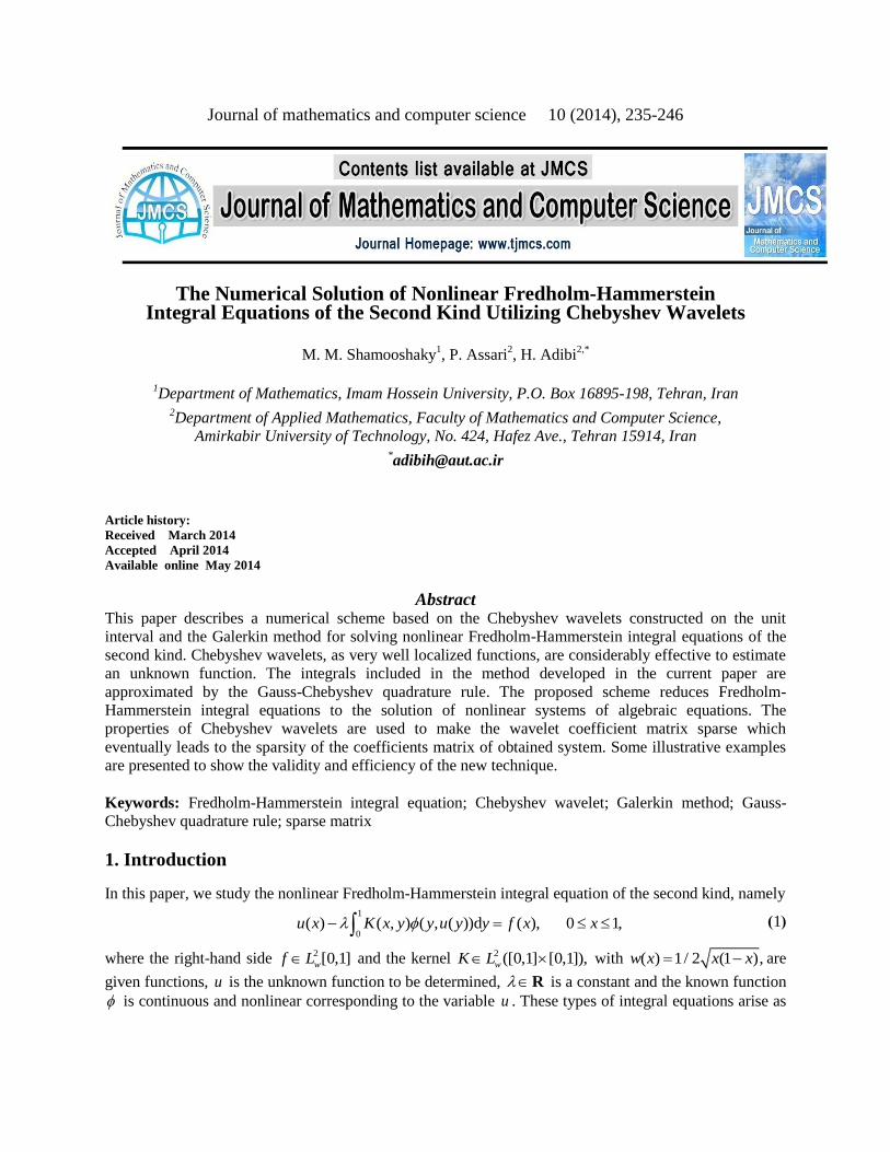
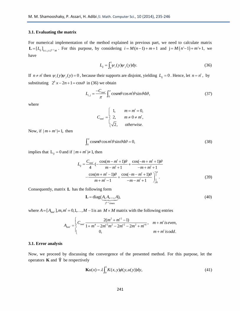
Example 4.2. In this example, we solve integral equation

by the present method, in which the exact solution is ( ) ex

exu x . It is seen the numerical results are

improved, as parameter k increases. All computations performed using the 10-point Gauss-Chebyshev

quadrature rule to approximate the integration numerically. Table 2 shows e

and 2

e at different

numbers of k and M and results are compared with [11]. Here, we put 5

0 10 for 2M and

4

0 10 for 3.M The approximation solution and absolute error for 4

06, 3, 10k M are shown

in Figure 2.

Table 2. Some numerical results for Example 4.2

k 2M 3M

method in [11] 2

e e

2

e e

2

3

4

5

6

21.71 10 34.34 10 31.05 10 42.76 10 53.24 10

25.13 10 21.42 10 31.61 10 49.52 10 42.05 10

48.05 10 41.01 10 51.27 10 61.32 10 71.99 10

33.21 10 44.31 10 55.81 10 67.22 10 79.34 10

13.23 10 28.07 10 23.23 10 35.61 10 31.93 10

e

1

0( ) e 0.382sin( ) 0.301cos( ) sin( )ln( ( ))d , 0 1,xu x x x x y u y y x


245

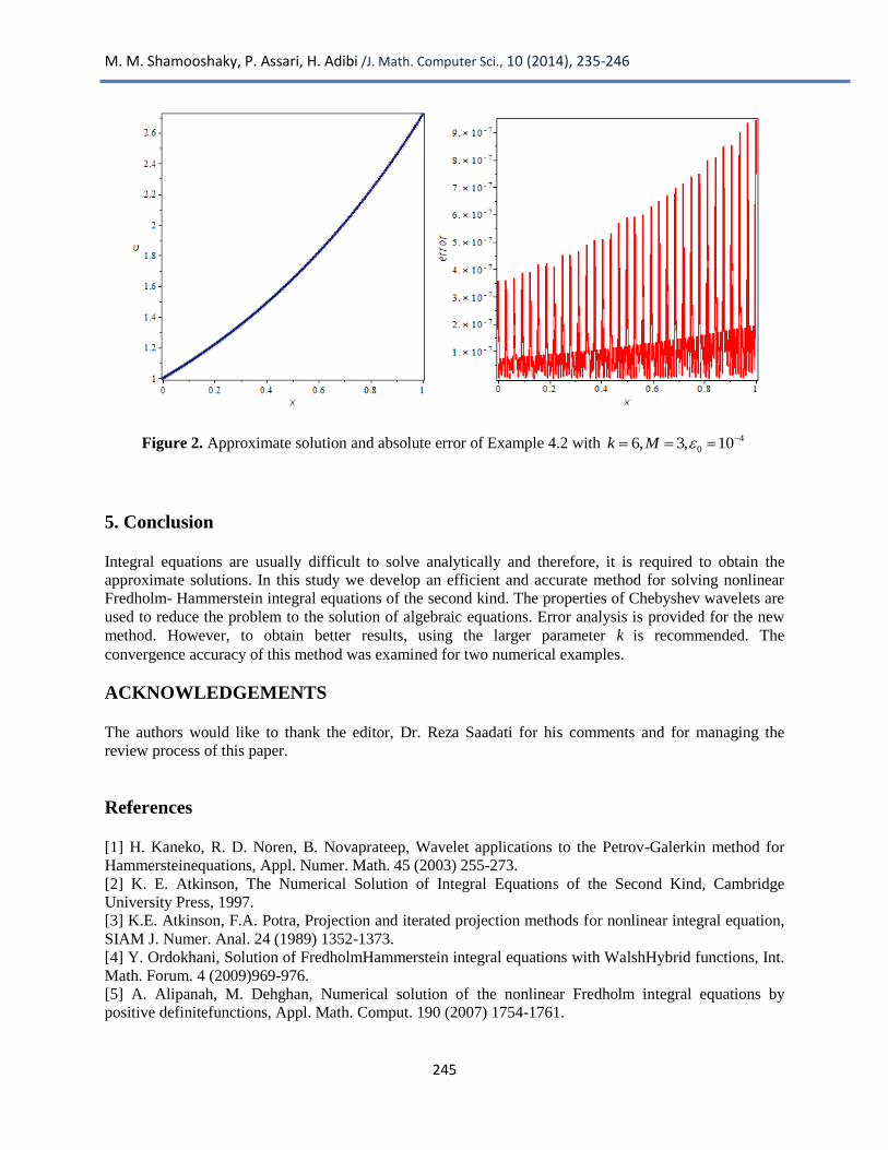
Figure 2. Approximate solution and absolute error of Example 4.2 with 4

06, 3, 10k M

5. Conclusion

Integral equations are usually difficult to solve analytically and therefore, it is required to obtain the

approximate solutions. In this study we develop an efficient and accurate method for solving nonlinear

Fredholm- Hammerstein integral equations of the second kind. The properties of Chebyshev wavelets are

used to reduce the problem to the solution of algebraic equations. Error analysis is provided for the new

method. However, to obtain better results, using the larger parameter k is recommended. The

convergence accuracy of this method was examined for two numerical examples.

ACKNOWLEDGEMENTS

The authors would like to thank the editor, Dr. Reza Saadati for his comments and for managing the

review process of this paper.

References

[1] H. Kaneko, R. D. Noren, B. Novaprateep, Wavelet applications to the Petrov-Galerkin method for

Hammersteinequations, Appl. Numer. Math. 45 (2003) 255-273.

[2] K. E. Atkinson, The Numerical Solution of Integral Equations of the Second Kind, Cambridge

University Press, 1997.

[3] K.E. Atkinson, F.A. Potra, Projection and iterated projection methods for nonlinear integral equation,

SIAM J. Numer. Anal. 24 (1989) 1352-1373.

[4] Y. Ordokhani, Solution of FredholmHammerstein integral equations with WalshHybrid functions, Int.

Math. Forum. 4 (2009)969-976.

[5] A. Alipanah, M. Dehghan, Numerical solution of the nonlinear Fredholm integral equations by

positive definitefunctions, Appl. Math. Comput. 190 (2007) 1754-1761.


246

[6] J. Rashidinia, M. Zarebnia, New approach for numerical solution of Hammerstein integral equations,

Appl. Math. Comput. 185 (2007) 147-154.

[7] K. Maleknejad, K. Nedaiasl, Application of Sinc-collocation method for solving a class of nonlinear

Fredholmintegral equations, Comput. Math. Appl. 62 (2011) 3292-3303.

[8] B.K. Alpert, A class of bases in L2 for the sparse representation of integral operators, SIAM J. Math.

Anal. 24 (1993) 246-262.

[9] H. Adibi, P. Assari, Using CAS wavelets for numerical solution of Volterra integral equations of the

second kind, Dyn. Contin.Discrete Impuls.Syst., Ser.A, Math.Anal. 16 (2009) 673-685.

[10] K. Maleknejad, K. Nouria, M. NosratiSahlan, Convergence of approximate solution of nonlinear

Fredholm-Hammerstein integral equations, Commun. Nonlinear. Sci. Numer. Simulat. 15 (2010) 1432-

1443.

[11] U. Lepik, E. Tamme, Solution of nonlinear Fredholm integral equations via the Haar wavelet

method, Proc. Estonian Acad. Sci. Phys. Math. 56 (2007) 17-27.

[12] H. Adibi, P. Assari, On the numerical solution of weakly singular Fredholm integral equations of the

second kind using Legendre wavelets, J. Vib. Control. 17 (2011) 689-698.

[13] E. Babolian, F. Fattahzadeh, Numerical solution of differential equations by using Chebyshev

wavelet operational matrix of integration, Appl. Math. Comput. 188 (2007) 417-426.

[14] E. Babolian, F. Fattahzadeh, Numerical computation method in solving integral equations by using

Chebyshevwavelet operational matrix of integration, Appl. Math. Comput. 188 (2007) 1016-1022.

[15] H. Adibi, P. Assari, Chebyshev Wavelet Method for Numerical Solution of Fredholm Integral

Equations of the First Kind, Math. Probl.Eng. 2010 (2010) 17 pages.

[16] S. Sohrabi, Comparison Chebyshev wavelet method with BPFs method for solving Abel's integral

equation. Ain.Shams. Eng. J. 2 (2011) 249-254.

[17] J. Biazar, H. Ebrahimi, Chebyshev wavelets approach for nonlinear systems of Volterra integral

equations, Comput. Math. Appl. 63 (2012) 608-616.

[18] L. Zhu, Q. Fan, Solving fractional nonlinear Fredholmintegro-differential equations by the second

kind Chebyshev wavelet, Commun. Nonlinear. Sci. Numer. Simulat. 17 (2012) 2333-2341.

[19] M. Ghasemi , M. AvassoliKajani, Numerical solution of time-varying delay systems by Chebyshev

wavelets. Appl. Math. Model.35 (2011) 5235-44.

[20] Y. Wang, Q. Fan. The second kind Chebyshev wavelet method for solving fractional di®erential

equations, Appl. Math.Comput. 218 (2012) 8592-8601.

[21] Y. Li, Solving a nonlinear fractional differential equation using Chebyshev wavelets, Commun.

Nonlinear. Sci. Numer. Simulat. 11 (2011) 2284-2292.

[22] I. Daubechies, Ten Lectures on Wavelets, SIAM/CBMS, Philadelphia PA, 1992.

[23] XuDinghua, Numerical Solutions for Nonlinear Fredholm Integral Equations of the Second Kind and

Their Superconvergence, J. Shanghai. Univ. 1 (1997) 98-104.

[24] S. Kumar, I. Sloan, A new collocation-type method for Hammerstein integral equations, Math.

Comput. 48 (1987) 585-593.

the numerical solution of nonlinear fredholm...

Documents