The nonlinear association between ENSO and the

Euro-Atlantic winter sea level pressure

Aiming Wu and William W. Hsieh

Dept. of Earth and Ocean Sciences, University of British Columbia

Vancouver, B.C., Canada, V6T 1Z4

Tel: (604) 822-3932, Fax: (604) 822-6088

E-mail: awu@eos.ubc.ca

Climate Dynamics

(revised)

July 14, 2004

1

Abstract

A nonlinear projection of the tropical Pacific sea surface temperature anomalies (SSTA) onto

the Northern Hemisphere winter sea level pressure (SLP) anomalies by neural networks (NN) was

performed to investigate the nonlinear association between ENSO and the Euro-Atlantic winter

climate. While the linear impact of ENSO on the Euro-Atlantic winter SLP is weak, the NN

projection reveals statistically significant SLP anomalies over the Euro-Atlantic sector during both

extreme cold and warm ENSO episodes, suggesting that the Euro-Atlantic climate mainly responds

to ENSO nonlinearly. The nonlinear response, mainly a quadratic response to the SSTA, reveals

that regardless of the sign of the SSTA, positive SLP anomalies are found over the North Atlantic,

stretching from eastern Canada to Europe (with anomaly center located just northwestward of

Portugal), and negative anomalies centered over Scandinavia and Norwegian Sea, consistent with

the excitation of the positive North Atlantic Oscillation (NAO) pattern.

2

1 Introduction

Numerous studies have been devoted to documenting and understanding the impact of the El Nino-

Southern Oscillation (ENSO) phenomenon on global climate variability since the early 1980s (Tren-

berth et al. 1998). An important progress on this issue made in recent years is that the extratropical

climate response to the tropical Pacific sea surface temperature (SST) anomalous forcing is found

to be nonlinear. Observational study and numerical models have demonstrated that North America

wintertime climate has asymmetric response patterns during opposite phases of ENSO (e.g. Shabbar

et al. 1997; Montroy et al. 1998; Hoerling et al. 1997, 2001a; Wu et al. 2003). A major characteristic

of North America climate response to ENSO is that there is an eastward phase shift of the circulation

anomalies (by about 35◦) between the composites of warm ENSO episodes and the composites of cold

episodes, with two wave trains originating from different tropical sources (Hoerling et al. 1997).

On the other hand, few studies have addressed the question if the impact of ENSO on the Euro-

Atlantic climate is nonlinear or not, partially because of the weaker and less robust relationship

between ENSO and the North Atlantic Oscillation (NAO, Hurrell et al. 2003). The impact of ENSO

on the atmospheric circulation in the North Atlantic region and the temperature in Europe has been

examined by some authors (e.g. Roger 1984; Fraedrich and Muller 1992; Fraedrich 1994; Halpert and

Ropelewski 1992; Huang et al. 1998; Dong et al. 2000; Sutton and Hodson 2003), but these studies

show varied, even contradictory results. For example, Rogers (1984) concluded from an analysis of

historical SLP data that there is no significant correlation between indices of the NAO and ENSO

on interannual and longer timescales. With a multiresolution cross-spectral technique, Huang et al.

(1998), however, found significant coherence between the NAO and Nino3 indices in about 70% of

the warm ENSO episodes from 1900 to 1995. Though there is some discrepancy in the location of

3

the atmospheric circulation anomalies, the studies by Pozo-Vazquez et al. (2001) and Cassou and

Terray (2001) both found no statistically significant sea level pressure (SLP) anomaly patterns in the

North Atlantic area associated with warm ENSO episodes, but both found a statistically significant

SLP anomaly pattern resembling the positive phase of the NAO during cold episodes. A cyclone

tracking analysis from a high resolution atmospheric general circulation model (AGCM) simulation

reveals a southward shift of the North Atlantic low pressure systems in the winter season during El

Nino episodes (Merkel and Latif 2002). The effects of different ocean conditions (including ENSO) on

the Northern Hemisphere midlatitude cyclone variability were also discussed by Raible and Blender

(2004).

In recent years, neural network (NN) methods have been increasingly applied to study the atmo-

sphere and oceans, with reviews given by Hsieh and Tang (1998) and Hsieh (2004). In this work,

the association between ENSO and the Euro-Atlantic climate is investigated by applying a nonlinear

projection of the ENSO SST index onto the Northern Hemisphere winter SLP. If x denotes the ENSO

SST index, and y, the extratropical atmospheric response to ENSO, the nonlinear response function

y = f(x) can be obtained via neural networks (Wu and Hsieh 2004) (the nonlinear projection by NN

is simply called an NN projection thereafter). In traditional linear projection, a linear regression of

the atmospheric response variable on the ENSO SST index, yields strictly anti-symmetric atmospheric

patterns during El Nino and La Nina (e.g. Deser and Blackmon 1995). In “one-sided regression”, one

calculates a linear regression between the SST index and the response variable when the SST index

is positive, and another linear regression when the SST index is negative (Hoerling et al. 2001a). In

contrast, the NN projection detects the fully nonlinear atmospheric response to ENSO. Compared to

the nonlinear canonical correlation analysis (NLCCA), developed also via NN (Hsieh 2001), the NN

projection has a much simpler NN structure with less model parameters, hence easier to obtain robust

4

results from noisy data. Composite analysis computes the atmospheric patterns by averaging the data

over the years when warm episodes occurred, and averaging over cold episodes. While the patterns

during warm and cold episodes are not forced to be anti-symmetrical, composite analysis does not

give a nonlinear response function.

The data and the method are briefly introduced in section 2. The nonlinear SLP anomaly patterns

associated with the ENSO SST index detected by the NN projection, and separately by a polynomial

fit are presented in section 3. Section 4 gives a summary and discussion.

2 Data and methodology

The monthly SLP data from January 1950 to March 2003 with a 5◦ by 5◦ resolution came from

the Trenberth Northern Hemisphere SLP data set (Trenberth and Paolino 1980). Anomalies were

calculated by subtracting the monthly climatology based on the period 1950-2002. Data from 20◦N to

the North Pole and during the winter season (December–March) were used, thus the total number of

months was 215. After removing the linear trend and weighting the anomalies by the square root of

the cosine of the latitude, a principal component analysis (PCA) was used to compress the data, with

the 11 leading principal components (PCs, accounting for about 83% of the total variance) retained.

Analysis using different number of PCA modes showed that our results were not sensitive to the

number of modes as long as 11 or more modes were used.

The spatial patterns of the four leading PCA modes (also called the empirical orthogonal functions,

EOFs) are shown in Fig. 1, where EOF1 (Fig. 1a) shows the typical Northern Annular Mode (NAM) or

the Arctic Oscillation (AO, Thompson and Wallace 1998, 2000), and EOF2 reveals strong variability

over North Pacific and a dipole structure between the North Atlantic and the Norwegian Sea (Fig. 1b).

5

The EOF3 shows SLP anomalies over the North Atlantic and Russia in opposition to the anomalies over

Greenland and Canada (Fig. 1c), while EOF4 displays anomalies over northern Europe in opposition

to the anomalies over the remaining mid-high latitude Northern Hemisphere (Fig. 1d).

The monthly SST for the period January 1950 to March 2003 with a resolution of 2◦×2◦ came

from the Extended Reconstructed Sea Surface Temperatures (ERSST) data set (Smith and Reynolds

2003). The SST anomalies were calculated by subtracting the monthly SST climatology based on the

period 1950-2002, and the linear trend removal was performed prior to PCA. The ENSO SST index is

defined as the standardized first PC of the winter (December–March) SSTA over the tropical Pacific

(122◦E-72◦W, 22◦S-22◦N). This ENSO SST index correlates strongly (>0.96) with the traditional

ENSO SST index of Nino3 and Nino3.4.

While the SST changes in the tropical Pacific have been found to be responsible for the rising

trend in the NAO index that was observed after 1950 (Hoerling et al. 2001b), we will focus on the

interannual to decadal time scales in this study as the linear trend has been removed from both the

SLP and SST data.

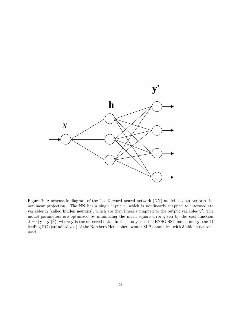
A schematic diagram of the feed-forward NN model is shown in Fig. 2. The NN has a single input,

the SST index (x), which is nonlinearly mapped to m intermediate variables called hidden neurons,

h = tanh(W(x)x + b(x)), where W(x) and b(x) are the weight and bias vector respectively (h, W(x)

and b(x) are column vectors of length m). The NN model then maps from the layer of hidden neurons

to 11 output variables y′ = W(h) · h + b(h), where W(h) is a 11 × m weight matrix, and b(h), a

bias vector of length 11. With enough hidden neurons, the NN is capable of modelling any nonlinear

continuous function to arbitrary accuracy (Bishop 1995). Starting from random initial values, the NN

model parameters (in W(x), b(x) W(h) and b(h)) are optimized so that the mean square error (MSE)

between the 11 model outputs (y′) and the 11 leading PCs (standardized) of the SLP anomalies (y)

6

is minimized. To avoid local minima during optimization, the NN model was trained repeatedly 30

times from random initial parameters and the solution with the smallest MSE was chosen and the

other 29 rejected.

To reduce the sampling dependence of a single NN solution, we repeated the above calculation

400 times with a bootstrap approach. A bootstrap sample was obtained by randomly selecting (with

replacement) one winter’s data record 54 times from the original record of 54 winters, so that on

average about 63% of the original record was chosen in a bootstrap sample (Efron and Tibshirani

1993). The ensemble mean of the resulting 400 NN models was used as the final NN solution, found

to be insensitive to the number of hidden neurons, which was varied from 1 to 5 in a sensitivity test.

Results from using 3 hidden neurons are presented.

3 Results

3.1 SLP response patterns extracted by NN projection

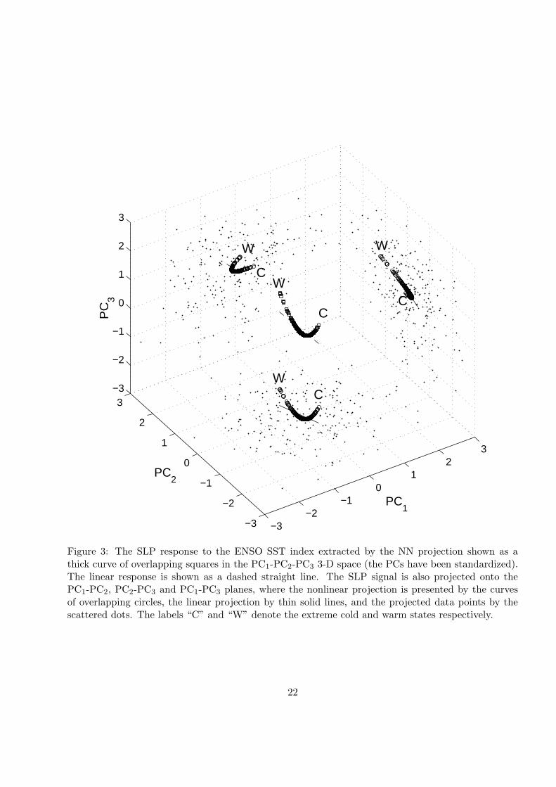
The climate signal extracted by the nonlinear projection is manifested by a curve in the 11 dimensional

phase space of the SLP PCs; in contrast, the linear projection extracts a straight line in the same 11-D

space. This curve was parabola-like (Fig. 3) when viewed in the PC1-PC2 plane and in the PC1-PC3

plane, indicating that the SLP response to the SST index is a nonlinear combination of some of its

leading PCA modes. For a given value of the SST index, the 11 SLP PC values derived from the

NN model can be combined with the corresponding EOFs (Fig. 1) to yield the SLP spatial anomalies

associated with this value of the SST index. As the SST index varies, both the pattern and amplitude

of the SLP spatial anomalies change, in contrast to the linear projection, which gives a fixed spatial

pattern and a variable amplitude.

7

When the SST index takes on its minimum value (i.e. strong La Nina), besides the positive SLP

anomalies over North Pacific (Fig. 4a), we see statistically significant positive SLP anomalies over

North Atlantic in a zonal belt stretching from the east coast of North America to western Europe,

and significant negative SLP anomalies over Scandinavia and Iceland, extending to eastern Europe,

resembling the positive phase of the NAO pattern, consistent with the composite SLP anomaly pattern

by Pozo-Vazquez et al. (2001). When the SST index takes on its maximum value (i.e. strong El Nino),

the positive SLP anomalies over North Pacific in Fig. 4a have turned into negative anomalies (Fig.

4b), with the anomaly center shifted eastward by 35◦ and with magnitude increased, confirming the

nonlinear impact of ENSO on the North Pacific and North America winter climate as documented

by previous studies (e.g. Hoerling et al. 1997). Meanwhile, the positive SLP anomalies over North

Atlantic are maintained and separated into two centers—one over eastern Canada, and the other one

over western Europe (Fig. 4b). Relative to the SLP pattern shown in Fig. 4a, Fig. 4b still displays a

positive NAO-like pattern over the Euro-Atlantic sector, but with the positive and negative anomaly

centers shifted eastward by about 15◦ and 30◦ respectively. Despite relatively weaker magnitude

and meridional gradient over North Atlantic and Europe in Fig. 4b compared to Fig. 4a, the NN

projection reveals significant SLP anomalies over the Euro-Atlantic region during strong warm ENSO

episodes, different from the composite analysis by Pozo-Vazquez et al. (2001), where no significant

SLP anomalies were found over North Atlantic during warm episodes. The similarity (or poor anti-

symmetry) in the SLP anomaly pattern over the Euro-Atlantic region between Figs. 4a and 4b suggests

a strong nonlinear relation between ENSO and the Euro-Atlantic winter climate.

Table 1 shows the PC values derived from the NN projection when the SST index takes on its

minimum and maximum values, where we see that large negative SST index values concur with large

positive PC1, small positive PC2, small negative PC3 and large positive PC4; while large positive

8

SST index values concur with small positive PC1, large positive PC2, intermediate positive PC3 and

small negative PC4. When the SST index varies from its minimum value to its maximum value, the

SLP response moves smoothly along the 3-D curve in Fig. 3 from the end labelled “C” to the other

end “W” (corresponding to the extreme cold and warm states respectively). From the corresponding

EOFs (Fig. 1), one can easily understand how the asymmetric SLP anomaly patterns arose during

the extreme cold and warm states as shown in Figs. 4a and 4b. Fig. 4a roughly resembles the positive

EOF1, while Fig. 4b is basically a combination of positive EOF2 and positive EOF3. The asymmetric

response between extreme cold and warm episodes is also contributed by higher modes although their

amplitudes are relatively small.

The SLP anomalies associated with the half minimum and half maximum SST index are shown

in Figs. 4c and 4d, respectively. The SLP anomalies decrease in magnitude, especially over the Euro-

Atlantic region. The anti-symmetry between Figs. 4c and 4d is much more conspicuous than that

between Figs. 4a and 4b, suggesting that appreciable SSTA are required for initiating the nonlinear

atmospheric response.

To estimate the nonlinear response in the SLP anomalies to the tropical SSTA, we plotted in

Fig. 4e the difference between the SLP anomalies in Fig. 4a and twice the anomalies in Fig. 4c; and

similarly in Fig. 4f, the difference between the anomalies in Fig. 4b and twice the anomalies in Fig. 4d.

Interestingly, despite the large difference between Figs. 4a and 4b, and the smaller difference between

Figs. 4c and 4d, the SLP anomalies in Figs. 4e and 4f agree well with each other, indicating that

regardless of the sign of the SST index, the nonlinear response has positive SLP anomalies appearing

over North Atlantic and western Europe, and negative SLP anomalies over Scandinavia and Iceland,

resembling a positive NAO pattern. In addition, we see negative SLP anomalies over the west coast of

North America and weak positive anomalies over eastern Canada, which contributes to the nonlinear

9

response of North America climate to ENSO.

To test the robustness of these results, we repeated our bootstrap calculations but deleting the

2 winters with the strongest ENSO warm episodes (1982-83, 1997-98), and the 2 winters with the

strongest cold episodes (1973-74, 1975-76) from the data record. Even without the extreme ENSO

episodes, the resulting NN projection yielded basically the same patterns as in Fig. 4. Another test

involved removing the 2 winters with the strongest positive NAO episodes (1958-59, 1988-89; selection

is based on the NAO index, i.e. the first PC of the SLP anomalies over Northern Hemisphere (Hurrell

et al. 2003)), and the 2 winters with the strongest negative NAO episodes (1968-69, 1976-77), which

also gave similar NN projection results, thereby confirming that the nonlinear response found by our

NN projection was not the result of fitting to one or two extreme cases.

3.2 The linear and nonlinear component of the SLP response

The SLP response to the ENSO SSTA as extracted by the NN projection can be separated into a

linear component, i.e. the linear projection (the straight line in Fig. 3), and a nonlinear component—

the residual after the linear projection subtracted from the NN projection, i.e. the 11 PCs from the

NN projection minus the 11 PCs from the linear projection. The resulting 11 PCs for the linear and

nonlinear components can then be combined with the corresponding EOFs to yield the linear and

nonlinear responses of SLP to ENSO. The linear and nonlinear components account for 65% and 35%

of the variance in the NN projected SLP anomaly data respectively.

PCA is used to separately analyze the linear and nonlinear response field of SLP anomalies during

Jan. 1950–Mar. 2003, where over 99% of the variance for either data field can be explained by its first

PCA mode. For the linear response field, the high percentage variance explained by the first PCA mode

is not surprising since the SLP anomalies field was generated originally by linearly projecting from a

10

single SST index time series. For the nonlinear response field, the high percentage variance explained

by a single PCA mode is due to the fact that the nonlinear response is very simple, consisting of mainly

a quadratic response, as will be shown later. When the PC1 of the linear response (the solid line in Fig.

5a) takes on a positive value, the EOF1 of the linear response (Fig. 5b) shows negative SLP anomalies

appearing over North Pacific and the west coast of North America continent, and weak positive SLP

anomalies over eastern Canada, with much weaker anomalies over Euro-Atlantic area, indicating the

linear impact of ENSO on the SLP over Euro-Atlantic sector is not important. However, the EOF1

of the nonlinear response (Fig. 5c) shows notable SLP anomalies over the Euro-Atlantic region, which

resemble a positive NAO pattern, and are similar to the SLP anomaly patterns shown in Figs. 4e and

4f, suggesting the Euro-Atlantic winter climate mainly responds to ENSO nonlinearly. The PC1 of

the linear response is synchronous with the ENSO SST index, while the PC1 of the nonlinear response

(the dashed line in Fig. 5a) has positive values not only during the El Nino winters (1958, 1966, 1973,

1983, 1992 and 1998), but also during La Nina winters (1950, 1956, 1971, 1974, 1976, 1989, 1999 and

2000). Hence, regardless of warm or cold episodes, the SLP has the same response pattern as depicted

by Fig. 5c. This leads to a positive NAO-like SLP pattern for both extreme cold and warm episodes

(Figs. 4a and 4b), showing the linear response (Fig. 5b) is weak over the Euro-Atlantic region.

The scatter plots between the PC1 of the nonlinear response and the SST index are shown in

Fig. 6 by the parabola-like curve of small solid circles, which can be fitted well by the polynomial

function PCNL1 = −7.37 − 1.55x + 8.28x2 − 0.54x3 − 0.19x4 + 0.01x5, where x is the ENSO SST

index, suggesting that the nonlinear response of SLP to ENSO is mainly a quadratic response. For

comparison, the scatter plot of the linear response is fitted well by the straight line PCLin1 = 13.65 x.

11

3.3 A polynomial study

To further illuminate the nonlinear response of the SLP anomalies, we consider a polynomial fit of

the SST index to the SLP anomaly at each grid point. Let T be the SST index, and xn = Tn,

then p, the original SLP anomaly at a grid point with linear trend removed, was fitted by p =

a0 + a1x1 + a2x2 + · · · + aN xN , where xn is xn normalized. For 400 bootstrap samples and for

each spatial point of the SLP anomaly field, regression coefficients a0, · · · , aN were computed. After

ensemble-averaging over all bootstrap samples, an provided the spatial pattern associated with the

nth order response to the SST index. When tested over independent data (i.e. data not selected in a

bootstrap sample), the smallest MSE (averaged over all bootstrap samples) was found when N = 2,

indicating overfitted results when N > 2. Hence there is no evidence for cubic or higher order nonlinear

response to ENSO. With N = 2, the ensemble-averaged values of a1 and a2 are plotted in Fig. 7.

Again the linear term has major SLP anomalies over North Pacific, and rather weak SLP anomalies

over the Euro-Atlantic region (Fig. 7a). In contrast, the quadratic term (Fig. 7b) shows major SLP

anomalies over Euro-Atlantic, resembling a positive NAO pattern, basically consistent with Fig. 5c,

as well as Figs. 4e and 4f, confirming that nonlinear response of SLP to ENSO is mainly a quadratic

response.

4 Summary and discussion

A fully nonlinear projection of the ENSO SST index to the Northern Hemisphere winter (December

to March) SLP monthly anomalies has been achieved using neural networks. Statistically significant

SLP anomalies resembling a positive NAO pattern are found over the Euro-Atlantic sector during both

extreme warm and cold episodes, except that the positive SLP anomaly center over the North Atlantic

12

is shifted eastward by approximately 15◦ during warm episode relative to that during cold episode.

The SLP anomalies from the NN projection consist of a linear part, which has anomalies largely

confined over North Pacific and the west coast of North America, and a nonlinear part, which has

major positive SLP anomalies over North Atlantic and western Europe, and negative SLP anomalies

over Scandinavia and Iceland, resembling the positive phase of the NAO pattern. A polynomial study

further indicates this nonlinear component to be a quadratic response to the SSTA. This manifestation

of the positive phase of the NAO during extreme warm and cold ENSO episodes was also found in the

winter 500 mb geopotential height anomalies (Wu and Hsieh 2004).

What needs to be emphasized is that, unlike the response of the North American climate to

ENSO, where the linear component is important, the response of the Euro-Atlantic climate to ENSO

is mainly nonlinear. This is probably why previous studies using linear analysis failed to obtain a

robust relationship between ENSO and NAO.

How the Euro-Atlantic climate anomalies are physically linked to the tropical Pacific ENSO SSTA

is still an open question. Just as its name implies, the Pacific-North America (PNA) teleconnection

(Wallace and Gutzler 1981), which is based on linear large-scale wave theory (Hoskins and Karoly

1981), cannot cover the Euro-Atlantic region (Fig. 5b and 7a). A possible mechanism is the wave-wave

interaction in the midlatitudes, e.g. the synoptic eddies and stationary waves. Merkel and Latif (2002)

showed that a high resolution AGCM, which can represent more realistically the transient eddy activity,

is necessary to simulate the cyclone variability related to ENSO over the North Atlantic/European

region. Although the physical process was not given in detail, their results agree with the our finding

here that the Euro-Atlantic climate is nonlinearly connected to ENSO. Thus the SST changes in the

tropical Pacific Ocean is still an important source for the predictability of the Atlantic and European

climate. The relative importance of the impact of ENSO SST and the Atlantic SST anomalies on the

13

Euro-Atlantic climate will be discussed in future work.

Acknowledgements

The authors acknowledge the support from the Natural Sciences and Engineering Research Council of

Canada via research and strategic grants.

14

References

Bishop CM (1995) Neural networks for pattern recognition. Clarendon Pr. Oxford.

Cassou C, Terray L (2001) Oceanic forcing of the wintertime low-frequency atmospheric variability in

the North Atlantic European sector: A study with the ARPEGE model. J Clim 14: 4266-4291

Deser C, Blackmon ML (1995) On the relationship between tropical and North Pacific sea surface

temperature variations. J Clim 8: 1677-1680

Dong B-W, Sutton RT, Jewson SP, O’Neill A, Slingo JM (2000) Predictable climate in the North

Atlantic sector during the 1997-1999 ENSO cycle. Geophys Res Lett 27: 985-988

Efron B, Tibshirani RJ (1993) An Introduction to the Bootstrap, CRC, Boca Raton.

Fraedrich K, Muller K (1992) Climate anomalies associated with ENSO extremes. Int J Climatol 12:

25-31

Fraedrich K (1994) An ENSO impact on Europe? Tellus 46A: 541-552

Halpert MS, Ropelewski CF (1992) Surface temperature patterns associated with the Southern Oscil-

lation. J Clim 5: 577-593

Hoerling MP, Kumar A, Zhong M (1997) El Nino, La Nina and the nonlinearity of their teleconnections.

J Clim 10: 1769-1786

Hoerling MP, Kumar A, Xu T (2001a) Robustness of the nonlinear climate response to ENSO’s extreme

phases. J Clim 14: 1277-1293

Hoerling MP, Hurrell J, Xu T (2001b) Tropical origins for recent North Atlantic climate change.

Science 292: 90-92

15

Hoskins B, Karoly D (1981) The steady linear response of a spherical atmosphere to thermal and

orographic forcing. J Atmos Sci 38: 1179-1196

Hsieh WW (2001) Nonlinear canonical correlation analysis of the tropical Pacific climate variability

using a neural network approach. J Clim 14: 2528-2539

Hsieh WW (2004) Nonlinear multivariate and time series analysis by neural network methods. Rev

Geophys 42, RG1003, doi:10.1029/2002RG000112

Hsieh, WW, Tang B (1998) Applying neural network models to prediction and data analysis in mete-

orology and oceanography. Bull Am Meteorol Soc 79: 1855-1870

Huang J-P, Higuchi K, Shabbar A (1998) The relation between the North Atlantic Oscillation and El

Nino-Southern Oscillation. Geophys Res Lett 25: 2707-2710

Hurrell JW, Kushnir Y, Ottersen G, Visbeck M (2003) An Overview of the North Atlantic Oscillation.

In: Hurrell JW, Kushnir Y, Ottersen G, Visbeck M (Eds) The North Atlantic Oscillation:

Climate Significance and Environmental Impact. Geophysical Monograph Series 134: 1-35

Merkel U, Latif M (2002) A high resolution AGCM study of the El Nino impact on the North At-

lantic/European sector. Geophys Res Lett 29: 1291-1294, doi: 10.1029/2001GL013726

Montroy DL, Richman MB, Lamb PJ (1998) Observed nonlinearities of monthly teleconnections be-

tween tropical Pacific sea surface temperature anomalies and central and eastern North American

precipitation. J Clim 11: 1812-1835

Pozo-Vazquez D, Esteban-Parra MJ, Rodrigo FS, Castro-Diez, Y (2001) The association between

ENSO and winter atmospheric circulation and temperature in the North Atlantic region. J Clim

14: 3408-3420

16

Raible CC, Blender R (2004) Northern hemisphere midlattitude cyclone variability in GCM simulations

with different ocean representations. Clim Dyn 22: 239-248, doi: 10.1007/s00382-003-0380-y

Rogers JC (1984) The association between the North Atlantic Oscillation and the Southern Oscillation

in the Northern Hemisphere. Mon Wea Rev 112: 1999-2015

Shabbar A, Bonsal B, Khandekar M (1997) Canadian precipitation patterns associated with Southern

Oscillation. J Clim 10: 3016-3027

Smith TM, Reynolds RW (2003) Extended reconstruction of global sea surface temperatures based on

COADS data (1854-1997). J Clim 16: 1495-1510

Sutton RT, Hodson DLR (2003) Influence of the Ocean on North Atlantic climate variability 1981-

1999. J Clim 16: 3296-3313

Thompson DWJ, Wallace JM (1998) The Arctic Oscillation signature in the wintertime geopotential

height and temperature fields. Geophys Res Lett 25: 1297-1300

Thompson DWJ, Wallace JM (2000) Annular modes in the extratropical circulation. Part I: Month-

to-month variability. J Clim 13: 1000-1016

Trenberth KE, Paolino DA (1980) The Northern Hemisphere sea level pressure data set: Trends, errors

and discontinuities. Mon Wea Rev 108: 855-872

Trenberth KE, Branstator GW, Karoly D, Kumar A, Lau N-C, Ropelewski C (1998) Progress during

TOGA in understanding and modelling global teleconnections associated with tropical sea surface

temperatures. J Geophys Res 103: 14291-14324

17

Wallace JM, Gutzler D (1981) Teleconnnection in the geopotential height filed durin the Northern

Hemisphere winter. Mon Wea Rev 109: 784-812

Wu A, Hsieh WW, Zwiers FW (2003) Nonlinear modes of North American winter climate variability

derived from a general circulation model simulation. J Clim 16: 2325-2339

Wu A, Hsieh WW (2004) The nonlinear Northern Hemisphere winter atmospheric response to ENSO.

Geophys Res Lett 31: L02203 DOI:10.1029/2003GL018885

18

Table 1: The standardized PC values derived from the NN projection when the ENSO SST indextakes on its minimum and maximum values. The standard deviation (STD) of the PCs is also given.

SLP PC STD NN(min) NN(max)

PC1 49.69 0.520 0.130

PC2 36.18 0.081 1.217

PC3 34.71 -0.117 0.382

PC4 31.28 0.656 -0.144

PC5 28.47 0.238 0.330

PC6 27.68 -0.379 0.419

PC7 23.41 -0.582 0.244

PC8 21.11 0.483 1.019

PC9 19.62 0.040 1.295

PC10 16.56 -0.045 -0.794

PC11 15.07 0.344 -0.158

19

Figure 1: The four leading empirical orthogonal functions (EOFs) of Northern Hemisphere winter(December–March) SLP anomalies. Solid curves denote positive contours, and dashed curves, negativecontours, and thick curves, the zero contours. The contour interval is 0.02. The EOFs have beennormalized to unit norm, and the percentage variance explained by each EOF is given in the figuretitle.

20

x

h

y'

Figure 2: A schematic diagram of the feed-forward neural network (NN) model used to perform thenonlinear projection. The NN has a single input x, which is nonlinearly mapped to intermediatevariables h (called hidden neurons), which are then linearly mapped to the output variables y′. Themodel parameters are optimized by minimizing the mean square error given by the cost functionJ = 〈‖y−y′‖2〉, where y is the observed data. In this study, x is the ENSO SST index, and y, the 11leading PCs (standardized) of the Northern Hemisphere winter SLP anomalies, with 3 hidden neuronsused.

21

−3−2

−10

12

3

−3

−2

−1

0

1

2

3−3

−2

−1

0

1

2

3

PC1

PC2

PC

3

C

C

C

C

W

W

W

W

Figure 3: The SLP response to the ENSO SST index extracted by the NN projection shown as athick curve of overlapping squares in the PC1-PC2-PC3 3-D space (the PCs have been standardized).The linear response is shown as a dashed straight line. The SLP signal is also projected onto thePC1-PC2, PC2-PC3 and PC1-PC3 planes, where the nonlinear projection is presented by the curvesof overlapping circles, the linear projection by thin solid lines, and the projected data points by thescattered dots. The labels “C” and “W” denote the extreme cold and warm states respectively.

22

Figure 4: The SLP anomalies associated with (a) the minimum SST index and (b) maximum SSTindex, and with (c) one half of the minimum SST and (d) one half of the maximum SST. The SLPanomalies in panel (a) minus twice the anomalies in (c) are shown in panel (e); and the anomalies inpanel (b) minus twice the anomalies in (d) are shown in panel (f). If the SLP response to the SSTindex is strictly linear, then (e) and (f) will show zero everywhere. Contour interval is 1 hPa and thegrey areas indicate statistical significance at the 5% level, based on the distribution of the results fromthe 400 bootstrap samples.

23

Figure 5: (a) The leading PC of the SLP anomalies from the linear and nonlinear response to the ENSOSST index as extracted by the NN projection, shown by the solid line and dashed line, respectively.The corresponding PCA spatial patterns for linear and nonlinear components are shown in panels (b)and (c), respectively. The contour interval is 0.03, and the spatial modes have been normalized tounit norm.

24

−3 −2 −1 0 1 2 3 4−30

−20

−10

0

10

20

30

40

50

ENSO INDEX

SLP

PC

1

Figure 6: The scatter plots between the ENSO SST index and the EOF PC1 of the nonlinear responseshown by the curve of small solid circles. The linear response is shown by the straight line of opencircles.

25

Figure 7: The SLP anomaly patterns associated with the (a) linear and (b) quadratic terms of thetropical Pacific SST index. The contour interval is 0.5 hPa and the shaded areas indicate statisticalsignificance at the 5% level from bootstrapping.

26