the new keynesian model and the small open economy … rbc model: equivalence results for...

The New Keynesian Model and the Small Open

Economy RBC Model: Equivalence Results for

Consumption

Dan Cao, Jean-Paul L’Huillier, Donghoon Yoo∗

December 2014

Abstract

We consider a modern New Keynesian model with “bells and whistles” (Chris-

tiano, Eichenbaum, and Evans 2005) with both permanent and temporary technology

shocks. We focus on the behavior of consumption and compare it to the one obtained

by the Small Open Economy RBC model (Schmitt-Grohe and Uribe 2003; Aguiar

and Gopinath 2007). We use the same (separable) preferences in both models. We

find that, for common parametrizations used in the respective literatures, consump-

tion behaves similarly in both models. Specifically, consumption is (almost) entirely

and solely determined by the long-run level of TFP: After a permanent impulse to

TFP, consumption (almost) jumps to that level and stays there. By the same logic,

consumption (almost) does not react to temporary TFP shocks. These results are

useful to interpret some quantitative results provided by these literatures.

Keywords: Consumption, DSGE, permanent income hypothesis, rigidities.

JEL codes: E10, E27, E37.

∗Georgetown University; Einaudi Institute for Economics and Finance (EIEF); EIEF and Tor Vergata.Dan thanks EIEF for hospitality and support during the preparation of this paper.

1

1 Introduction

Modern DSGE models are complex. They usually feature many ingredients

and parameters for which it is often difficult to derive precise results about the

equilibrium behavior of endogenous variables. In this paper, we consider close

versions of two widely used DSGEs in the literature and provide a simple and

sharp numerical characterization of the conditional dynamics of consumption.

The models we consider are the following. First, we take a modern version

of the New Keynesian model with so-called “bells and whistles” introduced

by Christiano, Eichenbaum, and Evans (2005) and later used by Smets and

Wouters (2007) and Justiniano, Primiceri, and Tambalotti (2010), among oth-

ers (henceforth NK-BW). Then, we consider the Small Open Economy RBC

model, originally introduced by Mendoza (1991), and subsequently used by

Schmitt-Grohe and Uribe (2003) and Aguiar and Gopinath (2007) (among oth-

ers), where the model features a debt-elastic interest-rate premium (henceforth

SOE-RBC). The only modification we introduce to the latter is that we use

the same preferences as in the NK-BW model. Both specifications only include

permanent and temporary technology shocks.

The first set of results we obtain is the following. We identify a param-

eter region, in both models, for which the behavior of consumption is solely

determined by the long-run level of Total Factor Productivity (TFP). Indeed,

after a persistent shock to TFP (which is modeled as the sum of an AR(1)

process in growth rates and a similar process in levels), consumption jumps to

the long-run level of TFP immediately when the initial permanent impulse hits.

That is, consumption is flat and features no fluctuations around the long-run

level of TFP. Also, by the same logic, consumption does not move after a tem-

porary technology shock. For both models, the parameter region features no

habit formation. Moreover, in the case of the NK-BW model, the parameter

region is one where a1) prices are very sticky or the interest rate rule is very

accommodative to inflation, and b1) the interest rule does not react to output.

In the case of the SOE-RBC model, the parameter region is one where a2) the

discount factor is close to one, b2) the elasticity of the interest premium is close

to zero, and c2) the steady state level of debt is zero1, with the requirement

that b2) holds more strongly than a2), i.e. the elasticity tends to zero faster

than the discount factor tends to one. We refer to this parametrization (for

1This last condition is not necessary for obtaining that consumption dynamics are flat, but they arenecessary to obtain that consumption jumps to the same level than long-run productivity.

2

each model respectively) by “limit parametrization”.

The parameter regions identified above are relevant because they are close

to standard parametrizations of both the NK-BW and SOE-RBC models in

the literature. These parametrizations are usually obtained by matching these

models to the data. In the case of the NK-BW model, Christiano et al. (2005)

estimate this model matching VAR-obtained IRFs to a monetary shock. In an-

other important paper, Smets and Wouters (2007) estimate the model through

Bayesian methods. Last but not least, Justiniano et al. (2010) estimate a model

with permanent instead of temporary shocks to TFP. In the case of the SOE-

RBC model, researchers usually focus on a calibrated version of the model. The

parametrization we consider is close to the calibration usually adopted, which

we refer to as “standard parametrization” for each model respectively. (In the

body of the paper we provide a detailed explanation of why we consider limit

and standard parametrizations close to each other.)2

The intuition for these results is straightforward and is given by the random-

walk permanent-income consumption model. In both parameter regions identi-

fied above the real interest rate is (almost) constant3, and therefore consumption

is determined by permanent income at all periods. In the NK-BW model, when

prices are very sticky inflation does not move, and therefore the rate determined

by the nominal interest rate rule does not move either (so long as the rate does

not react to output.) As a result, the real rate is constant. In the SOE-RBC

model, when the elasticity of the interest premium is small, the domestic real

interest rate is constant and equal to the foreign rate. Note that these findings

are not entirely obvious given that there are multiple differences between the

two models. To mention some of these differences, consider first goods markets.

The NK-BW model features monopolistic competition and Calvo price stick-

iness, while the SOE-RBC model features a competitive market with flexible

prices. In terms of labor markets, the NK-BW model features Calvo wage sticki-

ness and the SOE-RBC model features, again, a competitive market. Moreover,

the NK-BW model is closed economy, and the SOE-RBC is open economy. Be-

cause our limit parametrization is close to standard, our results imply that these

elements of the specification (among others not described) are largely irrelevant

for the conditional behavior of consumption after TFP shocks.

2Aguiar and Gopinath (2007) estimate a subset of parameters via method of moments, mainly concernedwith the stochastic shock processes. The parametrization above is close to the set of fixed parameters intheir paper.

3In a related paper, Kocherlakota (2012) studied the implications of a fixed real interest rate for labormarkets.

3

We rely on previously obtained theoretical results which form the basis for

our numerical exploration of the full-blown models mentioned above. The ran-

dom walk behavior of consumption was first established (to the best of our

knowledge) in Blanchard, L’Huillier, and Lorenzoni (2013) (Online Appendix

Section 6.4.2) in the case of a baseline New Keynesian model (Gali 2008). Sim-

ilar results were established in Cao and L’Huillier (2014b) (p. 11) for a Small

Open Economy RBC model without capital and inelastic labor. These theoret-

ical results help understand for instance why it is not required in the NK-BW

model to have the discount factor to be close to 1, whereas this is a requirement

in the SOE-RBC model. (We discuss these issues more in depth in the body of

the paper.)

The second set of results of the paper consists in showing that, for the usu-

ally adopted parametrization of both models in the literature, the consumption

implications of TFP shocks are similar in both models in the following sense.

We focus on the variance decomposition of consumption. We find that con-

sumption is almost entirely driven to permanent shocks. Given that here we

are not exactly in the parameter region identified above, the Impulse Response

Functions (IRFs) of consumption are no longer flat as before, but they are fairly

close to flat, and they look fairly similar in both models.

Our results are useful to understand some mechanics of consumption within

these models and to interpret some empirical results in the literature. We

discuss these interpretations after having presented our results in the conclusion.

The rest of the paper is organized as follows. The next Section lays down

both models. Section 4 presents first the optimality conditions of the models,

and then all numerical results. Section 5 concludes.

4

2 The Models

In this Section we present the models. We start by the elements common to both

models. We then specify the remaining elements of the NK-BW. Immediately

after we specify the remaining elements of the SOE-RBC model.

2.1 Elements Common to Both Models: Total Factor

Productivity and Preferences

Productivity at (in logs) is the sum of two components, permanent, xt, and

temporary zt

at = xt + zt (1)

The permanent component follows the unit root process

∆xt = ρx∆xt−1 + εt (2)

The temporary component follows the stationary process

zt = ρzzt−1 + ηt (3)

The coefficients ρx and ρz are in [0, 1), and εt and ηt are i.i.d. normal shocks

with variances σ2ε and σ2

η.

Preferences are given by

E

[∞∑t=0

βt(

ln (Ct − hCt−1)− 1

1 + ϕ

∫ 1

0

N1+ϕjt dj

)]

where Ct is consumption, the term hCt−1 captures internal habit formation,

and Njt is the supply of specialized labor of type j.

2.2 Remaining Specification of the NK-BW Model

The model is standard. The household budget constraint is

PtCt + PtIt + PtC(Ut)Kt−1 +Bt = Rt−1Bt−1 +

∫ 1

0

WjtNjtdj +RktKt

where Pt is the price level, It is investment, C(Ut) is the cost associated with

capital utilization in terms of current production, Kt is the stock of capital, Bt

5

are holdings of one-period bonds, Rt is the one-period nominal interest rate,

Wjt is the wage of specialized labor of type j, and Rkt is the capital rental rate,

and Kt are capital services rented (and used).

The capital stock Kt is owned and rented by the representative household

and the capital accumulation equation is

Kt = (1− δ) Kt−1 +

[1− χ

(ItIt−1

)]It

where adjustment costs in investment are captured by

χ

(I

I−

)=χ

2

(I

I−− 1

)2

The model features variable capital utilization and the capital services provided

by the capital stock Kt−1 are

Kt = UtKt−1

where Ut represents the degree of capital utilization. The cost associated with

capital utilization in terms of current production is given by

C(U) =1

1 + ξU1+ξ

Final good producers. The final good is produced using intermediate goods

with the CES production function

Yt =

[∫ 1

0

Y1

1+µp

it di

]1+µp

where µp captures a constant elasticity of substitution across goods.

Final good producers are perfectly competitive and maximize the profits

subject to the above production function, taking intermediate good prices Pit as

given and final good price Pt such that final good producers profit maximization

problem is

maxYit

PtYt −∫ 1

0

PitYitdi

Intermediate goods producers. There is a continuum of intermediate goods

producers where each producer produces good i with following production tech-

6

nology

Yit = Kαit (AtNit)

1−α

where Kit and Nit are capital and labor services employed and α ∈ (0, 1) repre-

sents capital’s share of output. As in the SOE-RBC model below, the parameter

At = eat .

Intermediate good prices are assumed to be Calvo-sticky. Each period inter-

mediate firm i can freely adjust the nominal prices with probability 1− θ and

firms that cannot adjust prices (with probability θ) set their price according to

Pit = Pit−1Πιt−1Π1−ι

where Π is the steady state level of inflation.

Labor markets. A representative competitive firm hires the labor supplied

by household j and aggregates the specialized labor supplied by the households

with the following technology

Nt =

[∫ 1

0

N1

1+µwjt dj

]1+µw

where µw is a constant elasticity of substitution among specialized labor.

Wages are Calvo-sticky. For each type of labor j, the household can freely

adjust the price Wjt with probability 1−θw and those that cannot adjust prices

(with probability θw) set their price according to

Wjt = Wjt−1

(Πt−1e

∆at−1)ιw

(Π)1−ιw

where Πt−1 is inflation at t− 1.

Monetary policy. Monetary policy follows the following interest rate rule

Rt

R=Rt−1

R

ρr((

Πt

Π

γπ)(

Yt/AtY/A

)γy)1−ρr

Market clearing. Market clearing in the final good market requires

Ct + It + C (Ut) Kt−1 = Yt

7

and market clearing in the market for labor services requires∫ 1

0

Njtdj = Nt

As Christiano et al. (2005), we define output gross of capital utilization costs.

2.3 Remaining Specification of the SOE-RBC Model

The specification is standard. Here, following the literature, there is no labor

heterogeneity and thus Njt = Nt.

Maximization of household utility is constrained by

Ct + It +Bt−1 = Yt +QtBt

where Ct, It and Yt are the consumption, investment, and output of the country,

Bt is the external debt of the country and Qt is the price of this debt.

Output is produced with capital and labor inputs through a Cobb-Douglas

production function

Yt = Kαt−1(AtNt)

1−α

where α ∈ (0, 1) represents capital’s share of output. The parameter At = eat .

The resource constraint is

Ct + It +NXt = Yt

where NXt are net exports. Following Aguiar and Gopinath (2007), the law of

motion for capital is

Kt = (1− δ)Kt−1 + It −ν

2

(Kt

Kt−1

− 1

)2

Kt−1

Capital depreciates at the rate δ, and the (quadratic) capital adjustment cost

is captured byν

2

(Kt

Kt−1

− 1

)2

Kt−1

Following Schmitt-Grohe and Uribe (2003) and Aguiar and Gopinath (2007),

among others, the price of debt is sensitive to the level of debt outstanding

1

Qt

= Rt = R∗ + ψ{eBtYt−b − 1

}8

where R∗ denotes the world interest rate, and b represents the steady state level

of the debt-to-output ratio.

9

3 Optimality Conditions and Steady State Con-

ditions

Following standards steps, we derive the optimality conditions (for both models)

and log-linearize. Here we present the FOC and deterministic steady state

relations for both models, which allows us to comment on the assumption that

the steady state level of debt in the SOE-RBC needs to be set to zero in order to

more easily compare across models (on p. 15). All details of the log-linearization

are given in the Appendix.

3.1 NK-BW Model: Optimality Conditions

Households. The FOC for consumption is

1

Ct − hCt−1

− βh 1

Ct+1 − hCt= Λt

where Λt is the multiplier of the budget constraint. The FOC for bond holdings

is

−Λt

Pt+ βRt

Λt+1

Pt+1

= 0

The FOC for investment

−Λt+Φt

[χ

(ItIt−1

− 1

)]+βΦt+1

[1− χ

2

(It+1

It− 1

)2

+χ

2

(It+1

It

)2(It+1

It− 1

)]= 0

where Φt is the multiplier for capital accumulation. The FOC for capital

Φt − βΛt+1C(Ut+1)− β (1− δ) Φt+1Kt = 0

Remain the budget constraint and the capital accumulation equation

Bt−1

PtRt−1 −

Bt

Pt+Wt

PtNt +

Rkt

PtKt − Ct − It − C(Ut)Kt−1 = 0

Kt − (1− δ)Kt−1 −

[1− χ

2

(ItIt−1

− 1

)2]It−1 = 0

The optimality condition for capacity utilization Ut is the solution to

maxUt

(Rkt /Pt

)UtKt−1 − C(Ut)Kt−1

10

which yields

Rkt /Pt = C ′(Ut) = ξU ξ

t

Final good producers. Final good producers maximize

maxYit

PtYt −∫ 1

0

PitYitdi

which gives the demand for intermediate good i

Yit = Yt

(PitPt

)− 1+µpµp

Since final good producer derives zero profit,

Pt =

[∫P

1µp

it di

]µpIntermediate goods producers. From the demand for intermediate good

Yit, µp is the constant markup for monopolist i. The cost minimization problem

for the monopolist is

minKit,Nit

RKt Kit +WitNit

subject to the production technology

Kαit (AtNit)

1−α = Yit

From the cost minimization problem, we obtain following FOCs:

Rkt −MCtαK

α−1it (AtNit)

1−α = 0

Wt −MCt (1− α)KαitA

1−αt N−αit = 0

Because of constant returns to scale all intermediate good firms choose the

same capital labor ratioKt

Nt

=α

1− αWt

Rkt

and the nominal cost of producing Yit is MCt · Yit where MCt is the marginal

cost

MCt =1

αα (1− α)1−α(Rkt

)α(Wt

At

)1−α

11

Calvo pricing implies that with probability (1 − θ) firms change price and

maximize

E

[∞∑s=0

θsβsΛt+s

Pt+s

(PitIt+s −MCt+s

)Yit+s

]where It+s is the indexing function

It+s = Πsk=1

(Πιpt+l−1Π1−ιp

)The optimality condition is then

E

[∞∑s=0

θsβsΛt+s

Pt+s

(1

µpIt+s −

1 + µpµp

MCt+sPit

)Yit+s

]= 0

Labor markets. Demand for variety j is

Njt = Nt

(Wjt

Wt

)− 1+µwµw

and the equilibrium wage is

Wt =

[∫W

1µwjt

]Calvo pricing for wage implies that with probability (1 − θw) workers can

adjust their wage and maximize

E

[∞∑s=0

θswβsΛt+s

Pt+s

(PjtIwt+sWjtNjt+s −

1

1 + φN1+φjt+s

)]

The optimality condition is then

E

[∞∑s=0

θswβsΛt+s

Pt+s

(1

µwIwt+s −

1 + µwµw

Nφjt+s

Wjt

)Njt+s

]= 0

3.2 NK-BW Model: Steady State Relations

We look for a steady state of stationary variables. This means that, because

of the unit root in at, we need to normalize some of the variables. We denote

steady state values by removing the time subindex.

12

From the intertemporal condition we obtain

R =Π

β

From the optimality condition for investment, we can see that

ΛA = ΦA

where ΛA is the multiplier multiplied by A, which is stationary, and similarly

for ΦA. In addition, the steady state value of the investment adjustment cost

is

χ (0) = 0

Also, in steady state

U = 1

so

C = 1

and from the Euler condition for capital we get

Rk/P =1

β− (1− δ)

where Rk/P is the steady state real rental rate. From optimality of prices

Pi/P = (1 + µp)MC/P

where MC/P are real marginal costs, and

Pi/P = 1

Thus

W/AP =

[αα (1− α)1−α

1 + µp

1

(Rk/P )α

]1/(1−α)

where W/AP are normalized real wages. From optimal factor combination, we

get

K/AN =α

1− αW/AP

Rk/P

where K/AN is the normalized capital-to-labor ratio. From the production

13

functionY

AN=

(K

AN

)αwhere Y/AN is the normalized output-to-labor ratio. From resource con-

straints, we have

I/AN = δK/AN

where I/AN is the normalized investment-to-labor ratio. Since

K/AN = K/AN

then

C/A = Y/A− I/A−K/A

3.3 SOE-RBC Model: Optimality Conditions

FOCs are obtained with respect to Ct, Nt, It, Kt, Bt,Λt,Φt, respectively:

Λt =1

Ct

(1− α)Λt = N1+ϕt

1

Yt

Λt + Φt = 0

Φt

[1 + ν

(Kt

Kt−1

− 1

)]+αβE

[Λt+1

(Yt+1

Kt

)]−βE

[Φt+1

((1− δ)− ν

2

(1−

(Kt+1

Kt

)2))]

= 0

QtΛt = βE[Λt+1]

Kαt−1(AtNt)

1−α − Ct − It +QtBt −Bt−1 = 0

Kt − (1− δ)Kt−1 − It +ν

2

((Kt

Kt−1

)2

− 1

)Kt−1 = 0

3.4 SOE-RBC Model: Steady State Relations

As in the NK-BW model, we look for a steady state of stationary variables. We

denote steady state values by removing the time subindex.

From the intertemporal condition, obtain the condition

R =1

β

14

The steady state ratio of capital to output can be obtained from the FOCs with

respect to Kt and It:K

Y=

α

1/β − (1− δ)From the capital accumulation equation we have

I

Y= δ

K

Y=

αδ

1/β − (1− δ)

The budget constraint gives

1− C

Y− I

Y= (1− β)

B

Y

The resource constraint gives

C

Y+I

Y+NX

Y= 1

From these steady state relations one can conclude that the steady state level

of current account surplus is given by

NX

Y= (1− β)

B

Y

Thus, in this model, the steady state level of normalized debtB/Y is determined

exogenously. For comparability of the model with the closed economy model

above, we assume B/Y = 0.

15

4 Results

We focus on the behavior of consumption in both the log-linearized NK-BW

model and the log-linearized SOE-RBC model (the log-linearization is presented

in the Appendix.) We consider two alternative parametrizations of both models.

Parametrization I is one in which the response of consumption is flat (limit

parametrization). Parametrization II is the typical one used in the literature

(standard parametrization). We obtain results for both parametrizations.

4.1 Limit parametrization

Parametrization I is shown in Table 1. This parametrization defines a parameter

region, for both models, in which the response of consumption is flat: it jumps to

the long-run level of TFP after a permanent shock, computed as the cumulated

sum of the growth rates implied by the shock, i.e.

a∞ =σε

1− ρx

and does not move after a temporary shock (because the long-run level of TFP

does not change after a temporary shock.)

The logic of this parametrization follows two theoretical results previously

obtained. We discuss the parametrization of the NK-BW model first, and then

we discuss the parametrization of the SOE-RBC model. We discuss the intuition

behind these choices after showing the results below. Blanchard, L’Huillier,

and Lorenzoni (2013) theoretically show (Online Appendix Section 6.4.2) that

a baseline NK model (without capital and no bells and whistles) converges to

a simple permanent income model with a fixed real interest rate and in which

consumption is equal to expectations of the long-run level of labor productivity.

We do not attempt to prove an equivalent theoretical result in the case of the

NK-BW model, but instead numerically obtain that the result generalizes to

this model as well. Following the conditions of the theorem proved in Blanchard

et al. (2013), we set in Parametrization I the Calvo parameter very close to 1.

We also set habit formation to 0 and we impose that the interest rate rule does

not react to output (both restrictions follow from the baseline NK model).

Regarding the SOE-RBC model, Cao and L’Huillier (2014b) theoretically

obtained the same result in the case of a small open economy model without

16

Table 1: Parametrization I (limit parametrization)

Parameter Value

Common to Both Models

h Consumption habit 0

α Capital share 0.17

ϕ Inv. Frisch elasticity 3.79

ξ Elasticity capital utilization cost 5.30

χ Investment adjustment costs 2.85

NK-BW Model

β Discount rate 0.9987

θ Calvo prices ≈1

θw Calvo wages 0.70

µ Price markup 0.23

µp Wage markup 0.15

γπ Taylor rule inflation 2.09

γy Taylor rule output 1× 10−7

φdy Taylor rule output growth 0

ι Price indexation 0.24

ιw Wage indexation 0.11

Policy

ρr Persistence nominal interest rate 0.82

SOE-RBC Model

β Discount rate ≈1

ψ Elasticity of the interest rate 1× 10−12

B/Y Steady state level of normalized debt 0

Shock Processes

Technology

ρx Persistence permanent shock 0.20

ρz Persistence temporary shock 0.20

σx Standard dev. permanent shock 1.00

σz Standard dev. temporary shock 1.00

Notes: Under this parametrization both models deliver flat responses of consumption. β for SOE-RBC model isset to 0.99999, and θ to 0.99999999.

17

capital and fixed labor supply4. We have a theoretical result of the model

including capital (Cao and L’Huillier 2014a), but the existing proof requires

fixed labor and uses the log-linearization adopted by Aguiar and Gopinath

(2007).5 We do not attempt to to prove an equivalent in the case of both

elastic labor supply and capital, but focus instead in numerical simulations.

Following the conditions of Proposition 1 in (Cao and L’Huillier 2014b), we

set the discount rate β close to 1, the elasticity of the interest rate ψ close to

0, and the ratio β/(1 − ψ) close to 0. (Specifically, we set β = 0.99999 and

ψ = 1× 10−12.)

The remaining structural parameters of the models are the estimates by

Justiniano et al. (2010). (They take a period to represent a quarter.) The

standard deviation of the shocks is normalized to 1, and their persistence is set

to 0.20.

Figure 1 shows the resulting behavior of TFP and consumption in both

models. We plot the IRFs of TFP and consumption following a permanent

and a temporary technology shock. In both cases, the response of consumption

is flat. The responses of consumption are indistinguishable from each other,

both models delivering similar responses. In the case of a permanent shock,

consumption jumps to the long-run level of TFP. In the case of a temporary

shock, consumption does not move.

The intuition for these results is straightforward and is given by the random-

walk permanent-income consumption model. In both parameter regions iden-

tified above the real interest is (almost) constant, and therefore consumption is

determined by permanent income at all periods. In the NK-BW model, when

prices are very sticky inflation does not move, and therefore the nominal in-

terest rate set by the nominal interest rate rule does not move either (so long

the rate does not react to output.) As a result, the real rate is constant.6 In

the SOE-RBC model, when the elasticity of the interest premium is small, the

domestic real interest rate is constant and equal to the foreign rate.

This intuition highlights the role of the consumption-Euler equation in de-

livering a flat consumption response. In particular, this also means that it is

needed to have separable preferences in order for the marginal utility for labor

not to enter the consumption-Euler equation. For non-separable preferences,

4Cao and L’Huillier (2013) contains a result in the case of elastic labor supply. This draft is availableupon request.

5This log-linearization is presented in the note by Aguiar and Gopinath (NA).6We obtain the same results by setting the reaction of the interest rate to inflation γπ close to 1 instead.

18

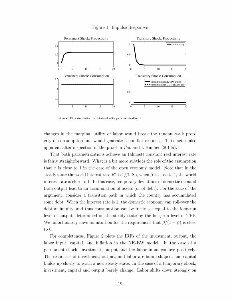
Figure 1: Impulse Responses

0 5 10 15 20

1

1.2

1.4

Permanent Shock: Productivity

0 5 10 15 20

0

0.5

1

Transitory Shock: Productivity

productivity

0 5 10 15 20

0.5

1

1.5Permanent Shock: Consumption

0 5 10 15 20

0

0.5

1

Transitory Shock: Consumption

consumption (NK−BW model)consumption (SOE−RBC model)

Notes: This simulation is obtained with parametrization I.

changes in the marginal utility of labor would break the random-walk prop-

erty of consumption and would generate a non-flat response. This fact is also

apparent after inspection of the proof in Cao and L’Huillier (2014a).

That both parametrizations achieve an (almost) constant real interest rate

is fairly straightforward. What is a bit more subtle is the role of the assumption

that β is close to 1 in the case of the open economy model. Note that in the

steady state the world interest rate R∗ is 1/β. So, when β is close to 1, the world

interest rate is close to 1. In this case, temporary deviations of domestic demand

from output lead to an accumulation of assets (or of debt). For the sake of the

argument, consider a transition path in which the country has accumulated

some debt. When the interest rate is 1, the domestic economy can roll-over the

debt at infinity, and thus consumption can be freely set equal to the long-run

level of output, determined on the steady state by the long-run level of TFP.

We unfortunately have no intuition for the requirement that β/(1− ψ) is close

to 0.

For completeness, Figure 2 plots the IRFs of the investment, output, the

labor input, capital, and inflation in the NK-BW model. In the case of a

permanent shock, investment, output and the labor input comove positively.

The responses of investment, output, and labor are hump-shaped, and capital

builds up slowly to reach a new steady state. In the case of a temporary shock,

investment, capital and output barely change. Labor shifts down strongly on

19

impact to compensate the productivity increase. Finally, inflation does not

move due to the high amount of price stickiness.

Figure 2: Impulse Responses: NK-BW model

0 5 10 15 20−2

0

2

4

6Investment

0 5 10 15 20−1

0

1

2Output

0 5 10 15 20−1

−0.5

0

0.5

1Labor Input

permanent shocktemporary shock

0 5 10 15 20−0.5

0

0.5

1

1.5Capital

0 5 10 15 20−0.1

−0.05

0

0.05

0.1Inflation


Figure 3 plots the IRFs of investment, output, the labor input, capital and

net exports in the SOE-RBC model. In the case of a permanent shock, in-

vestment and output comove positively. Capital accumulates, to reach a new

steady state in the long run. Net exports fall, and the labor input falls as well.

In the case of a temporary shock, investment and capital barely move. Output

increase temporarily, and this causes the domestic economy to save. The labor

input increases.

Another way to look into our results is to consider the variance decomposi-

tion in order to gauge which, among the permanent and the temporary shocks,

accounts for a higher proportion of consumption volatility. Figure 4 shows the

variance decomposition of the two models at different horizons. In both models,

(almost) all consumption volatility is accounted by the permanent shock.

4.2 Standard parametrization

Parametrization II is shown in Table 2. Here, we closely follow the literature.

All structural parameters of the NK-BW model are from the benchmark esti-

mation in Justiniano et al. (2010). Parameters specific to the SOE-RBC are set

as follows. The coefficient on interest rate premium, ψ, is set to 0.0010, which

20

Figure 3: Impulse Responses: SOE-RBC model

0 5 10 15 20−2

0

2

4Investment

0 5 10 15 200

0.5

1

1.5Output

0 5 10 15 20−0.2

0

0.2

0.4

0.6Labor Input


0 5 10 15 200

0.5

1

1.5Capital

0 5 10 15 20−1

−0.5

0

0.5

1Net Exports


Figure 4: Variance Decomposition

0 2 4 6 8 10 12 14 16 18 200.99

0.992

0.994

0.996

0.998

1

Periods

Var

ianc

e S

hare

(P

erm

anen

t Sho

ck)

NK−BW modelSOE−RBC model

Notes: Percentage of forecast error explained by the permanent shock. Per-centage of forecast error explained by temporary shock is just one minusthe variance share depicted here in the figure. The result is obtained withparametrization I.

21

is the number used in the literature (Schmitt-Grohe and Uribe 2003; Aguiar

and Gopinath 2007). The steady-state level of debt-to-output ratio B/Y is set

to 0.1 following Aguiar and Gopinath (2007). The standard deviation of the

shocks is normalized to 1, and their persistence is set to 0.20.

Parametrization II (the one used in the literature) is close to parametrization

I (the one that delivers exact flat responses of consumption). In the case of

the NK-BW model, most of the bells and whistles introduced by Christiano

et al. (2005) are real rigidities that, coupled with some nominal rigidity, form

a powerful force to obtain strong effects of nominal spending on output and

labor. At the same time, they allow consumption to be disconnected from

actual productivity by almost shutting down the general equilibrium effect on

the real interest rate. Thus, it is not crucial for our purposes that the Calvo

parameter θ tends to one: So long as it is fairly high, real rigidities will help

get an important effect of permanent shocks on consumption.

In the case of the SOE-RBC model, the usual parametrization naturally

picks a high discount rate. More importantly, general equilibrium effects on

consumption are muted by setting a small ψ (of around 0.001). As discussed

in the literature, ψ > 0 achieves stationarity of the debt holdings, however,

our analysis shows that setting it to a small value also disconnects consumption

from the rest of the model, pretty much as in a NK economy with sticky prices.7

Figure 5 presents the IRFs of productivity and consumption (in both models)

under parametrization II (upper and middle rows). The responses of consump-

tion are no longer flat, however, both models deliver very similar responses.

The non-flatness of the consumption responses is mostly due to the presence

of habit formation, which implies a slow upward adjustment of consumption

after a permanent shock. The bottom row of figures plots the responses under

parametrization II, but without habit formation, to show that the responses of

consumption are still fairly flat.

Figure 6 plots the IRFs of investment, output, the labor input, capital, and

inflation in the NK-BW model. The shape responses of investment, output

and capital are similar to the ones obtained under parametrization I. The labor

input now declines after a permanent shock. This is due to a smaller upward

reaction of output under the same increase in TFP, itself mainly due to a smaller

increase of consumption on impact. Inflation decreases after both shocks.

Figure 7 shows the IRFs of investment, output, the labor input, capital and

7See Garcia-Cicco, Pancrazi, and Uribe (2010) for a related feature of the model with small ψ in termsof the autocorrelation function of net exports.

22

Table 2: Parametrization II (standard parametrization)

Parameter Value

Common to Both Models

β Discount rate 0.9987

h Consumption habit 0.78

α Capital share 0.17

ϕ Inv. Frisch elasticity 3.79

ξ Elasticity capital utilization cost 5.30

χ Investment adjustment costs 2.85

NK-BW Model

θ Calvo prices 0.84

θw Calvo wages 0.70

µ Price markup 0.23

µp Wage markup 0.15

γπ Taylor rule inflation 2.09

γy Taylor rule output 0.07

φdy Taylor rule output growth 0.24

ι Price indexation 0.24

ιw Wage indexation 0.11

Policy

ρr Persistence nominal interest rate 0.82

SOE-RBC Model

ψ Elasticity of the interest rate 0.0010

B/Y Steady state level of normalized debt 0.1

Shock Processes

Technology

ρx Persistence permanent shock 0.20

ρz Persistence temporary shock 0.20

σx Standard dev. permanent shock 1.00

σz Standard dev. temporary shock 1.00

Notes: Parametrization based on Justiniano, Primiceri, and Tambalotti (2010), Schmitt-Grohe and Uribe (2003),and Aguiar and Gopinath (2007).

23

Figure 5: Impulse Responses

0 5 10 15 20

1

1.5Permanent Shock: Productivity

0 5 10 15 200

0.5

1

Transitory Shock: Productivity

productivity

0 5 10 15 20

0.5

1

1.5Permanent Shock: Consumption

0 5 10 15 200

0.5

1

Transitory Shock: Consumption


0 5 10 15 20

0.5

1

1.5Permanent Shock: Consumption w/o Habit

0 5 10 15 200

0.5

1

Transitory Shock: Consumption w/o Habit


Notes: This simulation is obtained with parametrization II.

Figure 6: Impulse Responses: NK-BW model

0 5 10 15 20−1

0

1

2

3Investment

0 5 10 15 20−0.5

0

0.5

1

1.5Output

0 5 10 15 20−1

−0.5

0

0.5Labor Input


0 5 10 15 20−0.5

0

0.5

1Capital

0 5 10 15 20−0.1

−0.05

0

0.05

0.1Inflation


24

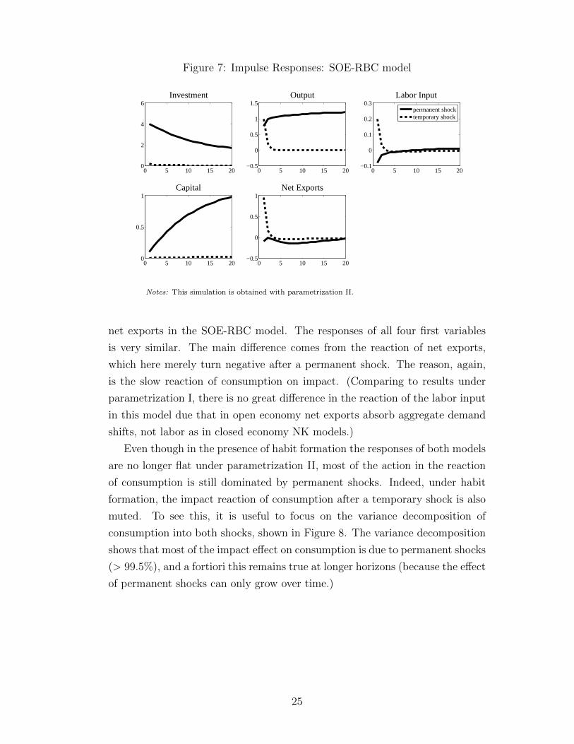
Figure 7: Impulse Responses: SOE-RBC model

0 5 10 15 200

2

4

6Investment

0 5 10 15 20−0.5

0

0.5

1

1.5Output

0 5 10 15 20−0.1

0

0.1

0.2

0.3Labor Input


0 5 10 15 200

0.5

1Capital

0 5 10 15 20−0.5

0

0.5

1Net Exports


net exports in the SOE-RBC model. The responses of all four first variables

is very similar. The main difference comes from the reaction of net exports,

which here merely turn negative after a permanent shock. The reason, again,

is the slow reaction of consumption on impact. (Comparing to results under

parametrization I, there is no great difference in the reaction of the labor input

in this model due that in open economy net exports absorb aggregate demand

shifts, not labor as in closed economy NK models.)

Even though in the presence of habit formation the responses of both models

are no longer flat under parametrization II, most of the action in the reaction

of consumption is still dominated by permanent shocks. Indeed, under habit

formation, the impact reaction of consumption after a temporary shock is also

muted. To see this, it is useful to focus on the variance decomposition of

consumption into both shocks, shown in Figure 8. The variance decomposition

shows that most of the impact effect on consumption is due to permanent shocks

(> 99.5%), and a fortiori this remains true at longer horizons (because the effect

of permanent shocks can only grow over time.)

25

Figure 8: Variance Decomposition

0 2 4 6 8 10 12 14 16 18 200.99

0.992

0.994

0.996

0.998

1

PeriodsV

aria

nce

Sha

re (

Per

man

ent S

hock

)

NK−BW modelSOE−RBC model

Notes: Percentage of forecast error explained by permanent shock. Per-centage of forecast error explained by temporary shock is just one minusthe variance share depicted here in the figure. The result is obtained withparametrization II.

5 Conclusions

This paper has numerically identified a parameter region for both a modern New

Keynesian model (Christiano, Eichenbaum, and Evans 2005) and the small open

economy RBC model (Schmitt-Grohe and Uribe 2003; Aguiar and Gopinath

2007) in which the random-walk permanent income property of consumption

holds. We demonstrate this by studying the behavior of consumption condi-

tional on both permanent and temporary shocks to TFP. At the limit, the

real interest rate is (almost) fixed. The parameter region identified is rele-

vant because it is quite close to standard parametrizations of the NK-BW and

SOR-RBC models in the literature.

In terms of choices, we decided to execute these exercises using the same

preferences in both models. This choice was motivated by clarity and focus on

general equilibrium effects of the economy. However, this is not such a strong

restriction because we could have defined the above limit parameter region by

setting σ = 1 in the preferences

ut =[Cγ

t (1− Lt)1−γ]1−σ

1− σ(4)

which are those used by Aguiar and Gopinath (2007) and are also considered by

Schmitt-Grohe and Uribe (2003) (p. 117). When σ = 1, (4) become log-log and

then separability implies that we would obtain the same results, as discussed

in the body.

We believe our results shed some light on some findings of the literature

and improve our understanding of the role of some of the ingredients employed

26

by researchers. First, we have established that temporary TFP shocks are

not useful to move consumption. Many DSGE models feature only temporary

(stationary) TFP shocks, thus there is need to use other shocks in order to

explain consumption volatility. Some popular alternatives are preference shocks

(in the form of shocks to the discount factor), or noise shocks (Lorenzoni 2009).

Second, permanent TFP shocks are clearly more able to move consumption,

especially on impact. It is possible that this result is useful in order to get

a volatile and countercyclical current account movements in an open economy

RBC model, as studied by Aguiar and Gopinath (2007). However, in this paper

we have not explored the exact parametrization employed by these authors.

Exploring this link more carefully seems like a fruitful research avenue.

References

Aguiar, M. and G. Gopinath (2007). Emerging market business cycles: The

cycle is the trend. Journal of Political Economy 115 (1), 69–102.

Aguiar, M. and G. Gopinath (N/A). Log-linearization notes. Unpublished .

Blanchard, O. J., J.-P. L’Huillier, and G. Lorenzoni (2013). News, noise,

and fluctuations: An empirical exploration. American Economic Re-

view 103 (7), 3045–3070.

Cao, D. and J.-P. L’Huillier (2013). Technological revolutions and debt hang-

overs: Is there a link? Mimeo.

Cao, D. and J.-P. L’Huillier (2014a). The behavior of consumption in the

RBC open economy model. Mimeo.

Cao, D. and J.-P. L’Huillier (2014b). Technological revolutions and the three

great slumps: A medium-run analysis. Mimeo.

Christiano, L. J., M. Eichenbaum, and C. L. Evans (2005). Nominal rigidities

and the dynamic effects of a shock to monetary policy. Journal of Political

Economy 113 (1), 1–45.

Gali, J. (2008). Monetary policy, inflation and the business cycle: An intro-

duction to the New Keynesian framework. Princeton: Princeton Univer-

sity Press.

Garcia-Cicco, J., R. Pancrazi, and M. Uribe (2010). Real business cycles in

emerging countries? American Economic Review 100 (5), 2510–2531.

Justiniano, A., G. Primiceri, and A. Tambalotti (2010). Investment shocks

27

and business cycles. Journal of Monetary Economics 57 (2), 132–145.

Kocherlakota, N. R. (2012). Incomplete labor markets. Mimeo.

Lorenzoni, G. (2009). A theory of demand shocks. American Economic Re-

view 99 (5), 2050–84.

Mendoza, E. G. (1991). Real business cycles in a small open economy. Amer-

ican Economic Review 81 (4), 797–818.

Schmitt-Grohe, S. and M. Uribe (2003). Closing small open economy models.

Journal of International Economics 61, 163–185.

Smets, F. and R. Wouters (2007). Shocks and frictions in US business cycles:

A bayesian DSGE approach. American Economic Review 97 (3), 586–606.

28

A Log-linear Approximation

A.1 NK-BW Model

First we define log-deviations for variables in the approximation. Here we also

normalize variables in the model to ensure their stationarity. Specifically, we

define

ct ≡ log(Ct/At)− log(C/A))

We define in a similar way yt, kt, kt, and it. Nt and Ut are already stationary,

therefore we define

nt ≡ log(Nt)− log(N)

ut ≡ log(Ut)− log(U)

For nominal variables, we also need to consider non-stationarity in the price

level and therefore define

wt ≡ log ((Wt/Pt) /At)− log ((W/P ) /A)

rkt ≡ log(Rkt /Pt)− log

(Rk/P

)rt ≡ log(Rt)

πt ≡ log(Pt/Pt−1)− Π

Finally, for Lagrange multipliers, we define

λt ≡ log(ΛtAt)− log(ΛA)

φt ≡ log(ΦtAt/Pt)− log(ΦA/P )

Households. The marginal utility of consumption is

Λt =1

Ct − hCt−1

− βh 1

Ct+1 − hCt

multiplying both sides by At

ΛtAt =1

Ct/At − h (Ct−1/At−1) (At−1/t)−βh 1

(Ct+1/At+1) (Ct+1/At)− h (Ct/At)

29

which with log-linearization yields

λt =hβ

(1− hβ) (1− h)Etct+1 −

1 + h2β

(1− hβ) (1− h)ct +

h

(1− hβ) (1− h)ct−1+

(5)

+hβ

(1− hβ) (1− h)Et∆at+1 −

h

(1− hβ) (1− h)∆at

The Euler equation is

Λt = βRtEt[Λt+1

PtPt+1

]Multiplying both sides of this Euler equation by At gives

ΛtAt = βRtEt[Λt+1At+1

AtAt+1

PtPt+1

]and approximating yields

λt = rt + Et [λt+1 −∆at+1 − πt+1] (6)

The optimality condition for capacity utilization is

Rkt /Pt = U ξ

t

In logs,

rkt = ξut (7)

The provision of the capital services is

Kt = UtKt−1

dividing both sides by At

Kt

At=UtAt

¯Kt−1

At−1

At−1

At

Approximating it leads to

kt = ut + kt−1 −∆at (8)

30

The capital accumulation equation is

Kt = (1− δ) Kt−1 +

[1− χ

2

(ItIt−1

− 1

)]It

dividing both sides by At

Kt

At= (1− δ) Kt−1

At−1

(At−1

At

)+

[1− χ

2

(ItIt−1

− 1

)]ItAt

Approximating this leads to

K

A

(1 + kt

)= (1− δ) K

A

(1 + kt+1 −∆at

)+

[1− χ

2

(ItIt−1

)2]I

A(1 + it)

which summarizes to

K

A

(1 + kt

)= (1− δ) K

A

(1 + kt+1 −∆at

)+I

A(1 + it)

Then, the log-linear approximation is

kt = (1− δ)(kt+1 −∆at

)+ δit (9)

The optimality condition for capital is

Φt − βΛt+1C(Ut+1)− β (1− δ) Φt+1Kt

which is log-linearly approximated to

φt = (1− δ) βEt [φt+1 −∆at+1] + [1− (1− δ) β]Et[λt+1 −∆at+1 + rkt+1

](10)

Similarly, for the optimality condition for investment

−Λt+Φt

[χ

(ItIt−1

− 1

)]+βΦt+1

[1− χ

2

(It+1

It− 1

)2

+χ

2

(It+1

It

)2(It+1

It− 1

)]= 0

The log-linear approximation obtained is

λt = φt − χ (it − it−1 + ∆at) + βχEt [it+1 − it + ∆at+1] (11)

31

Final good producers. Total output

Yt = Kαt (AtNt)

1−α

dividing both sides by AtYtAt

=Kαt

AαtN1−αt

Taking logs,

yt = αkt + (1− α)nt (12)

Intermediate goods producers. The optimal factor proportions between

capital and labor isKt

Nt

=α

1− αWt

Rkt

rearranging and dividing both sides by At,

(1− α)Kt

AtRkt = α

Wt

AtNt

Log-linearizing it leads to

kt − nt = wt − rkt (13)

The marginal cost equation is

MCt =1

αα (1− α)1−α(Rkt

)α(Wt

At

)1−α

dividing both sides by Pt

MCtPt

=1

αα (1− α)1−α

(Rkt

Pt

)α(Wt

PtAt

)1−α

Log-linearizing, it leads to

mct = αrkt + (1− α)wt (14)

Finally, from the optimality conditions for price setters, we have

πt =ι

1 + ιβπt−1 +

β

1 + ιβEtπt+1 + κmct (15)

where κ = (1− θβ) (1− θ) /θ (1 + ιβ).

32

Labor market. Similar to the optimality conditions for price setters, aggre-

gating individual optimality conditions for the wage setter lead to

wt =1

1 + βwt−1 +

β

1 + βEtwt+1 +

ιw1 + β

πt−1 −1 + ιwβ

1 + βπt +

β

1 + βEtπt+1 (16)

+ιw

1 + β∆at−1 −

1 + ιwβ

1 + β∆at +

β

1 + βEt∆at+1 − κwmcwt

where

kw =(1− θwβ) (1− θw)

[θ (1 + β) (1 + ϕ (1 + 1/µw))]

and

mcwt = wt − ϕnt + λt (17)

Monetary policy. The interest rate rule is

Rt

R=

(Rt−1

R

)ρr [(Πt

Π

γπ)(

Yt/AtY/A

)γy]1−ρr ( Yt/AtYt−1/At−1

)φdywe obtain

rt = ρrrt−1 + (1− ρr) (γππt + γyyt) + φdy (yt − yt−1) (18)

Market clearing Market clearing in goods market implies

C (1) = Rk/P

and

Ct + It + C (Ut) Kt−1 = Yt

Dividing both sides by At and approximating

C

Act +

I

Ait +

RkK

PAut =

Y

Ayt

which leads to

yt =C

Yct +

I

Yit +

RkK

PYut (19)

33

A.1.1 Summary

• There are 18 variables in the model. The endogenous variables are

λt, φt, yt, ct, it, kt, kt, nt, ut, rt, rkt , wt, πt,mct,mc

wt

and the exogenous variables are

at, xt, zt

• Equations (1)-(3) and (5)-(19) constitute the log-linearized model.

A.2 SOE-RBC Model

In order to log-linearize the model, we define the following log-deviations:

ct ≡ log(Ct/At)− log(C/A))

yt ≡ log(Yt/At)− log(Y/A))

kt ≡ log(Kt/At)− log(K/A))

it ≡ log(It/At)− log(I/A))

nt ≡ log(Nt)− log(N)

λt ≡ log(ΛtAt)− log(ΛA)

φt ≡ log(ΦtAt)− log(ΦA)

the log of the interest rate

rt ≡ log(Rt)

and the following absolute deviations:

bt ≡Bt

Yt− B

Y

nxt ≡NXt

Yt− NX

Y

In addition to the ten endogenous variables defined above, we also have addi-

tional exogenous variables xt, zt, at summarizing the productivity process. Log-

linearization of the equilibrium conditions proceeds as follows. The marginal

34

utility of consumption is

Λt =1

Ct


λt =AtCt

where λt = ΛtAt. In logs the condition is

λt = −ct (20)

The production function is

Yt = Kαt−1 (AtNt)

1−α

dividing both sides At

YtAt

=

(Kt−1

At−1

)α(At−1

At

)αN1−αt

The log-linearized production function is

yt = αkt + (1− α)nt − α∆at (21)

The resource constraint is

Ct + It +NXt = Yt

multiplying both sides by Yt

CtAt

AtYt

+ItAt

AtYt

+NXt

Yt= 1

Since in steady stateC

A

A

Y+I

A

A

Y+NX

Y= 1

approximating,

C

A

A

Y(1 + ct − yt) +

I

A

A

Y(1 + it − yt) + nxt +

NX

Y= 1

which yieldsC

Y(ct − yt) +

I

Y(it − yt) + nxt = 0 (22)

35

The price of debt equation is

Rt = R∗ + ψ(eBtYt−b − 1

)We have steady state relation

R = R∗

so approximating the equation yields

rt = ψbt (23)

The optimality condition for labor is

(1− α)Λt = N1+ϕt

1

Yt


(1− α)λt = N1+ϕt

AtYt

In logs

λt = (1 + ϕ)nt − yt (24)

The budget constraint

Ct + It +Bt−1 = Yt +QtBt

dividing both sides by Yt,

CtAt

AtYt

+ItAt

AtYt

+Bt−1

Yt−1

AtYt

Yt−1

At−1

At−1

At= 1 +Qt

Bt

Yt

which leads in steady state

C

A

A

Y+I

A

A

Y+B

Y= 1 +Q

B

Y

Approximating

C

A

A

Y(1+ct−yt)+

I

A

A

Y(1+it−yt)+(bt−1 + b) (1−∆yt −∆at) = 1+

1

R(1− rt) (bt + b)

36

Since 1/R = β, we have that

C

Y(ct − yt) +

I

Y(it − yt) = βbt − bt−1 + b(∆at + yt − yt−1 − βrt) (25)

The optimality condition for debt is

QtΛt = βEt [Λt+1]

multiplying both sides by At,

Qtλt = βEt[λt+1

(AtAt+1

)]which in steady state

1 = βR

Then, approximating

λt = Et [λt+1 −∆at+1] + rt (26)

The optimality condition for investment is

Λt = −Φt


λt = −φt (27)

The capital accumulation equation is

Kt − (1− δ)Kt−1 − It +ν

2

((Kt

Kt−1

)2

− 1

)Kt−1 = 0

multiplying both sides by At,

Kt

At− (1− δ)Kt−1

At−1

At−1

At− ItAt

+ν

2

((Kt

At

At−1

Kt−1

AtAt−1

)2

− 1

)Kt−1

At−1

At−1

At= 0

which in steady state

δK

A− I

A= 0

Then, approximating

(1+kt)−(1−δ) (1 + kt−1 −∆at)−I

K(1 + it)+

ν

2(1 + kt−1 −∆at)

((1 + kt − kt−1 + ∆at)

2 − 1)

= 0

37

which yields

kt = (1− δ) [kt−1 −∆at] + δit (28)

Finally, the optimality condition for capital is

Φt

[1 + ν

(Kt

Kt−1

− 1

)]+αβEt

[Λt+1

(Yt+1

Kt

)]−βEt

[Φt+1

((1− δ)− ν

2

(1−

(Kt+1

Kt

)2))]

= 0


φt

[1 + ν

(Kt

Kt−1

− 1

)]+ αβEt

[λt+1

AtAt+1

(Yt+1

Kt

)]−

−βEt

[φt+1

AtAt+1

((1− δ)− ν

2

(1−

(Kt+1

Kt

)2))]

= 0

which in steady state is

φ+ αβEt[λY

K

]− βEt [φ (1− δ)] = 0

Approximating, we end up with

φ (1 + φt) [1 + ν (1 + kt) (1− kt−1) (1 + ∆at)− ν] +

+αβλ (1 + λt+1) (1−∆at+1) (1 + yt+1) (1− kt) (1 + ∆at+1)Y

K+

+βφ (1 + φt+1) (1−∆at+1) [− (1− δ))− ν (kt+1 − kt + ∆at+1)] = 0

which yields after collecting terms

−(1 + φt + νkt − νkt−1 + ν∆at) + αβY

K(1− kt + Et [yt+1 + λt+1])+ (29)

+β(1− δ)(1 + Et [φt+1 −∆at+1])− β(νkt − Et [νkt+1 + ν∆at+1]) = 0

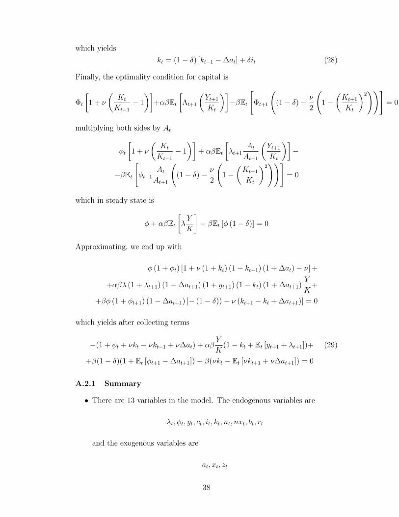
A.2.1 Summary

• There are 13 variables in the model. The endogenous variables are

λt, φt, yt, ct, it, kt, nt, nxt, bt, rt

and the exogenous variables are

at, xt, zt

38

• Equations (1)-(3) and (20)-(29) constitute the log-linearized model.

39

the new keynesian model and the small open economy … rbc model: equivalence results for...

Documents