The Need for (long) Chains in Kidney Exchange

Itai Ashlagi David Gamarnik Michael A. Rees Alvin E. Roth∗

May 21 2012

Abstract

It has been previously shown that for sufficiently large pools of patient-donor pairs,

(almost) efficient kidney exchange can be achieved by using at most 3-way cycles,

i.e. by using cycles among no more than 3 patient-donor pairs. However, as kidney

exchange has grown in practice, cycles among n > 3 pairs have proved useful, and long

chains initiated by non-directed, altruistic donors have proven to be very effective. We

explore why this is the case, both empirically and theoretically.

We provide an analytical model of exchange when there are many highly sensi-

tized patients, and show that large cycles of exchange or long chains can significantly

increase efficiency when the opportunities for exchange are sparse. As very large cy-

cles of exchange cannot be used in practice, long non-simultaneous chains initiated by

non-directed donors significantly increase efficiency in patient pools of the size and com-

position that presently exist. Most importantly, long chains benefit highly sensitized

patients without harming low-sensitized patients.

1 Introduction

Kidney exchange arises because a healthy person has two kidneys and can donate one to

a person in need of a transplant, but a donor and his or her intended recipient may be

incompatible. An incompatible patient-donor pair can exchange with another pair, or with

more than one other pair, in a cycle of exchanges among patient-donor pairs that allows each

patient to receive a kidney from a compatible donor. In addition, sometimes exchange can

∗Ashlagi: iashlagi@mit.edu. Gamarnik: gamarnik@mit.edu. Rees: Michael.Rees2@utoledo.edu Roth:

al roth@harvard.edu. Dr. Rees is the medical director of the Alliance for Paired Donation. We thank

Gabriel Caroll, Vivek Farias, Jacob Leshno, Parag Pathak, Alex Woltizky and the participants in the MIT-

Harvard economic theory seminar for valuable suggestions and comments. This work has been partially

supported by the National Science Foundation.

1

be initiated by a non-directed donor (an altruistic donor who does not designate a particular

intended patient), and in this case a chain of exchanges need not form a closed cycle.

The present paper seeks to understand why such chains have become increasingly impor-

tant in practical kidney exchange. We will see that the answer has to do with the growing

percentage of patients for whom finding a compatible donor is difficult. For such patients,

the “coincidence of wants” needed to find a short cycle of exchanges becomes a rare event,

and chains go a long way towards lifting the constraint that a cycle of exchanges needs to

satisfy. In the conclusion we will explore briefly how this may have implications for other

kinds of barter economies and markets with liquidity constraints. (It is illegal in the U.S.

and in most of the world to buy or sell organs for transplantation.)1

Roth et al. (2004) proposed a way to organize kidney exchange, integrating cycles and

chains. Due to incentive and logistical constraints, cycles need to be of small size. Initially

clearinghouses organized cycles involving no more than 2 patient-donor pairs (Roth et al.

(2005a,b)), and even today cycles often involve no more than 3 pairs (since a 3-way cycle

involves the simultaneous coordination of 6 operating rooms and surgical teams).2

All the surgeries in a cyclic exchange are conducted essentially simultaneously because,

in a cycle, every patient-donor pair both gives a kidney and receives one, and so the cost

of a broken link would be very high to a pair that first donated a kidney and later failed

to receive one.3 It is this requirement of simultaneity that makes large cycles so demanding

logistically.

Roth et al. (2006) proposed that the growing number of non-directed donors would allow

the simultaneity constraint to be relaxed. When a chain is initiated by a non-directed donor,

it can be organized so that the non-directed donor makes the initial donation, and no patient-

donor pair has to donate a kidney before they have received one. Since this reduces the cost

1See Roth (2007) on repugnant transactions. Recall that Jevons (1876) proposed that money was invented

as a market design solution to overcome precisely the difficulties of organizing barter economies–in particular,

the low volume of trade that could be expected through barter because of the difficulty of satisfying the

“double coincidence” of wants involved in simultaneous 2-way cycles. Computer-assisted clearinghouses for

kidney exchange are an attempt to organize a barter economy on a large scale.2Roth et al. (2007) showed that, when patients are not too highly sensitized and the pool of pairs is

sufficiently large, cycles of size greater than 4 can often be decomposed into cycles of length no larger than

three. Finding as many transplants as possible using two or three way cycles is a hard computational problem

and Abraham et al. (2007) have proposed an algorithm that works in practice for finding cycles in relatively

large size exchange pools.3Not only would such a pair have undergone a surgery that did them no benefit, but they would also have

lost the donor’s kidney and so not be in a position to participate in a future kidney exchange. Conducting

the exchange simultaneously ensures that no donor gives a kidney until all the donors have been successfully

prepared for surgery. Saidman et al. (2006) and Roth et al. (2007) studied efficient allocation when only

cyclic exchanges are available.

2

of a broken link, such chains can be organized non-simultaneously, which allows them to be

longer, as more operating rooms and surgical teams can be assembled over a longer time.4

Particularly after the publication of Rees et al. (2009), which reported the initial ten

transplants from the first nonsimultaneous chain, a growing number of long nonsimultaneous

chains have been conducted. However there is an ongoing debate about whether long chains

increase efficiency beyond simultaneous small cycles (see Gentry et al. (2009), Ashlagi et al.

(2011a), Gentry and Segev (2011), Ashlagi et al. (2011b)).5 One reason that long chains

might not increase efficiency is if they simply accomplished transplants that could otherwise

have been accomplished in multiple short cycles.

The empirical part of this paper examines the patient-donor pairs enrolled in one of the

earliest kidney exchange clearinghouses, the Alliance for Paired Donation (APD), and shows

that allowing long chains significantly increases efficiency. The key for this finding is the

high percentage of highly sensitized patients in the data. Patients are highly sensitized if

(for reasons other than blood type incompatibility) the probability that any donor’s kidney

will be compatible for them is low; i.e. highly sensitized patients are those for whom finding

a transplantable kidney will be difficult, even from a donor with the same blood type,

because of tissue-type incompatibilities. We will see that long chains increase the number

of transplants that can be achieved, by increasing the number of highly sensitized patients

who can receive transplants.

Efficiency in kidney exchange has been studied previously. Roth et al. (2007) model a

large market by assuming that compatibility between a patient and a donor of two distinct

incompatible pairs in the exchange pool is determined merely according to blood types and

show that 4-way cycles are sufficient for efficiency.6 Unver (2010) showed a similar result in a

dynamic setting. Ashlagi and Roth (2011) (see also Toulis and Parkes (2011)) showed similar

results as above dropping the assumption that only blood type determines compatibility, i.e.

taking more explicit account of the fact that the more sensitized a patient, the less likely

he or she will be compatible with a random donor. Roth et al. (2007) used simulations to

show that even on small exchange pool sizes of 25–100 patient-donor pairs, limiting cycles

to at most size 3 hardly results in any efficiency loss. Although these papers do not study

4Ausubel and Morrill (2010) consider a model with sufficiently many pairs so that there is no remaining

uncertainty, and consider nonsimultaneous chains in which patient-donor pairs donate before receiving a

kidney, in return for a reliable promise of receiving one later.5At the same time, news stories report how a single non-directed donor can initiate a chain of transplants

that saves many lives (see e.g. http://marketdesigner.blogspot.com/search/label/chains for stories about

chains involving up to 60 surgeries–30 nephrectomies and 30 transplants).6The idea behind this assumption is that if a patient is compatible with a constant fraction of donors, then

as the donor pool grows large there will be many compatible donors. As will become clear, the patient-donor

pools we will be concerned with here are not large in this way.

3

efficiency in the presence of non-directed donors, it can be easily derived from these results

that any non-directed donor can add at most 3 transplants to the number of matches in

sufficiently large markets (see Figure 1 and Section 4.1).

These results seem to settle the efficiency problem, at least for exchange pools that

grow without limit. Existing clearinghouses, however, operate with relatively small pools of

patient-donor pairs. In three different exchange pools with which we have worked (one of

which is examined in detail here), we find that limiting the maximum size of cycles to 3 and

even 4 results in a significant loss of transplants. And when even one non-directed donor is

in the pool, finding long chains together with cycles of at most size 3 can yield many more

transplants than using only cycles limited to size 3 (see Table 2).

One should expect that the empirical percentage of highly sensitized patients in the ex-

change pool will be higher than the percentage of highly sensitized patients in the general

patient population since almost all patients presently enrolled in exchange pools are incom-

patible with their donors, and many are tissue-type incompatible. However the observed

percentage of highly sensitized patients is much higher than the percentage of highly sensi-

tized patients that arise in simulations that generate incompatible pairs using the sensitivity

distribution of the general population (see for example the simulations used by Roth et al.

(2007)).7 Our empirical findings about the usefulness of long chains and larger exchanges are

a direct result of highly sensitized pools – small cycles that include a highly sensitized pa-

tient are rare, because highly sensitized patients can receive kidneys from only a few donors,

which makes the double coincidence needed for e.g. a 2-way cycle unlikely. In a related

paper, Ashlagi et al. (2011a) use simulations, also based on clinical data, to show that long

chains increase efficiency in a dynamic setting (see also Ashlagi et al. (2011b)).89

Based on our empirical findings, we provide here a theoretical framework for studying

highly sensitized exchange pools. We focus on the immunological (tissue-type) incompat-

ibilities that make some patients highly sensitized and difficult to match. For clarity, in

Section 4 we will model patient-donor pairs who are all blood type compatible and show,

when patients are highly sensitized, how important large cycles become even in the absence

of blood type incompatibility.10 We focus on the role played by the sparsity of the compati-

7In those simulations, a patient was drawn according to the general population distribution, then a donor

and the patient join the exchange pool only if they are incompatible.8Understanding the causes of the empirical distribution of sensitivity of patients in the exchange pools is

an important topic for future research. At least one cause is that hospitals do not fully participate in kidney

exchange programs, for example by not revealing easy to match pairs that they can transplant through

internal cycles (see Ashlagi and Roth (2011), Ashlagi et al. (2010) and Toulis and Parkes (2011) who study

how to prevent this problem by redesigning the mechanism).9Dickerson et al. (2012) further confirm the results by Ashlagi et al. (2011a) that long chains increase

efficiency in dynamic settings.10The important role that blood types play in efficiently matching pairs in dense compatibility graphs is

4

bility graph. Most importantly, we show that the highly sensitized patients are the ones to

benefit from moving to longer cycles and chains, and that this does not harm low-sensitized

patients. We further show how the analytical results are consistent with the matchings that

can be constructed from the existing patient data.11 Our results explain why chains are

proving to be so useful, how much they add to efficiency, and why a non-directed donor can

often initiate a very long chain that includes many otherwise hard to match patient-donor

pairs.

2 A model for kidney exchange

In an exchange pool there are patients with kidney failure, each paired with an incompatible

living donor,12 and also non-directed donors. The set of incompatible pairs and non-directed

donors (NDDs), V , induces a compatibility graph DV which captures the compatibilities

between donors and patients in the pool. The set of nodes is V , and for any two nodes

v, u ∈ V , there is a directed edge from u to v if and only if the donor of node u is compatible

with the patient of node v.

A k-way cycle (k > 0) involves k incompatible pairs v1, v2, . . . , vk such that for every

i, 1 ≤ i < k, the donor of vi is compatible with the patient of vi+1 and the donor of vk is

compatible with the patient of v1, i.e. there is a path v1, v2, . . . , vk, v1 in the graph.

In practice the size of a cycle is limited (mostly due to logistical constraints). We assume

there is an exogenous maximum size limit k > 0 for any cycle. Thus if k = 3, only cycles of

size 2 and 3 can be conducted.13

Although cycles of size more than 3 are seldom used in practice due to simultaneity

constraints, chains, initiated by a non-directed donor can be conducted non-simultaneously

and thus can be of any size. A k-way chain (k > 0) involves a non-directed donor v0 and k

now well understood. When patients are not highly sensitized, it is especially straightforward to show that

short cycles are sufficient to match all pairs in which patient and donor have the same blood type, but we

will see that this is no longer the case when patients are highly sensitized.11The comparison with the data serves two purposes: it shows that we analytically model a realistic level

of sparsity, and that our analytical results for large graphs, holding sparsity fixed, depend on the sparsity

rather than the size of the graph, and apply to clinically relevant size patient populations of the indicated

sparsity.12Pairs that are compatible would presently go directly to transplantation and not join the exchange pool

(but see e.g. Roth et al. (2005) and Sonmez and Unver (2011) on the advantages of changing this policy).13In two of the exchanges with which we have worked, the Alliance for Paired Donation (APD) and the

New England Program for Kidney Exchange (NEPKE), k was originally set to 2, was increased to 3, and now

optimization is conducted over even larger cycles and chains. The pilot national program initially considered

cycles up to size 3. Cycles are generally conducted simultaneously, so a cycle of size k requires 2k operating

rooms and surgical teams for the k nephrectomies (kidney removals) and k transplants.

5

incompatible pairs v1, v2, . . . , vk such that for every i, 0 ≤ i < k the donor of vi is compatible

with the patient of vi+1, i.e. there is a path v0, v2, . . . , vk in the graph.14

An allocation is a set of distinct exchanges. An allocation M is called (k, l)-efficient if

it achieves the maximum number of transplants possible using only cycles of size no more

than k and chains of size no more than l. It is called k-efficient if it is (k, 0)-efficient, and

is called efficient if it is (k, l)-efficient for unbounded k and l.

In the next section we study efficient allocations for different maximum cycle and chain

lengths, in data from a kidney exchange program, which, like all the kidney exchange pro-

grams with which we are familiar, includes many highly sensitized, hard to match patients.

We shall see that contrary to previous analytical results and simulations, cycles up to size

3 and even 4 are not sufficient for full efficiency, and long cycles and/or chains prove to be

very effective for increasing the number of transplants.

3 Empirical efficiency

The empirical data we present here are from the Alliance for Paired Donation (APD) clear-

inghouse (we found similar results in data sets from other clearinghouses). Each patient

has a level of percentage reactive antibodies (PRA) which measures the probability that

the patient will be incompatible with a random donor, even if that donor has a compatible

blood type. The lower the PRA of a patient, the more likely the patient is compatible with

a random donor. In their simulations, Roth et al. (2007) use a PRA distribution which is

taken from the UNOS data for the general patient population on the waitlist for deceased

donor kidneys (see the first column in Table 1). Three intervals are described as, low PRA

(0-9%), medium (10-79%) and high (80-100%).

In all data sets we estimate the PRA by observing for each patient the number of blood

type compatible donors he or she is also tissue-type compatible with. Table 1 provides the

estimated distributions. The first and second column describe the PRA distributions in

UNOS and the resulting PRA distribution from simulations that have been done in previous

studies (how pairs were generated is described below). The next three columns report the

distribution of the historical set of incompatible pairs in APD (i.e. the set of all pairs enrolled

through its history prior to October 2011) and two different snapshots (that capture the pairs

enrolled at two different moments in time, and hence all available to be matched to each

other). The number of patient-donor pairs in the data sets are: 361,131,144 respectively.15

14One can model chains begun by non-directed donors as (cyclic) exchanges by associating each non-

directed donor with an artificial virtual patient who can receive a kidney from any other donor in the pool.15Dickerson et al. (2012) also mention that almost all 77 patients in the the UNOS pilot program which

launched in 2010 are highly sensitized. We also observed a similarly high percentage of high PRA patients

6

UNOS Previous simulations Historical APD set 1st APD set 2nd APD set

Size 361 131 144

Low PRA 90.19 0.87 48.20 34.36 40.2

High PRA 9.81 0.13 51.80 65.64 59.8

Table 1: Percentages of Low and High PRA patients in various data sets and standard simulations.

Naturally the PRA distributions in the kidney exchange data sets will differ from the

PRA distribution in UNOS since low PRA patients are easier to match and therefore less

likely to join the pool. One way to generate a PRA distribution that is more realistic

is by generating incompatible pairs as follows: generate a patient, generate a potential

donor for this patient, and simulate a crossmatch test. The donor patient pair is added to

the exchange pool only if they are incompatible. Such a process was used in Roth et al.

(2007), Ashlagi et al. (2011a) and Ashlagi and Roth (2011). More highly sensitized patient

pools can be simulated if each patient can have several potential donors, and the patient

and one of her donors joins the pool only if the patient and all her potential donors are

incompatible. Simple simulations/calculations (using the PRA distribution as in Roth et al.

(2007)) show that to reach the level of the sensitivity in the data, patients need to have

available and be incompatible with many potential donors; for example if each patient is

tested and found incompatible with 5 potential donors the pool will contain approximately

58% highly sensitized patients.

The very high percentage of high PRA patients in the exchange pool makes compatibility

graphs sparse, implying that short cycles and short chains might not be sufficient. We looked

at the allocations in each of these sets allowing various maximum exchange sizes. The results,

reported in Table 2, show that by limiting cycles to size 3 and even 4 there is a substantial

efficiency loss.16

To summarize, we find that larger cycles and long chains are needed for efficiency in

exchange pools of the size and composition we are seeing in clinical settings.

One question that is thus becoming important for the design of kidney exchange clear-

inghouses is why is there such a big gap between the PRA distribution predicted from the

general patient population and the empirical PRA distribution enrolled in exchange pools.

At least part of the answer has to do with hospitals not revealing their easy to match pairs

to the exchange pools (see Ashlagi and Roth (2011)), resulting in a higher fraction of highly

in data sets from other kidney exchange clearinghouses with which we have worked.16Ashlagi and Roth (2012) report related results in simulated data. Manlove and O’Malley (2012) observe

that allowing 4-way cycles (and not just 2 and 3-ways) is also likely to increase efficiency in the UK kidney

exchange.

7

k = 2 k = 3 k = 4 k = 5 k =∞ (3,∞) (∞,∞) (3, 5)

Historical APD set 118 169 189 191 193 194.25 194.25 172

1st APD set 6 9 11 13 16 17.3 17.3 10.1

2nd APD set 8 12 16 16 16 17.9 17.9 14.1

Table 2: Allocations in Data. In the first 5 columns, we report the size of the k-efficient allocation where

∞ stands for unrestricted k. In the last 3 columns the average size of the (k, l)-efficient allocation is given

using a single non-directed donor that is chosen at random, i.e. the average size of maximum allocation

using cycles up to size k and a chain up to size l.

sensitized patients in the pool.

An additional factor that adds to this gap is the accumulation of very highly sensitized

patients over time due to the dynamic nature of exchange programs; consider for example a

very highly sensitized patient p in the pool who can receive a kidney from a donor d who is

also currently in the the pool. If p and d cannot be part of a 2-way or a 3-way cycle, d may

take part in a different exchange, leaving the highly sensitized patient p behind in the pool.

A related question is, what causes the big difference between the efficiency results ob-

tained by Roth et al. (2007) and Ashlagi and Roth (2011) for dense graphs, and the empirical

efficiency results we show here? We will see that this is a direct consequence of the highly

sensitized pool, which implies that the compatibility graphs are sparse, and not dense.

In the next section we motivate and adopt a new stylized model based on Erdos-Renyi

random graphs, to study highly sensitized pools.

4 Random compatibility graphs

To analyze efficiency, the previous studies focused on blood type incompatibilities, either

explicitly or implicitly. Ashlagi and Roth (2011) analyzed random compatibility graphs that

are generated from both blood-type and tissue type distributions consistent with practice.

In this paper we simplify the distribution from which the graph is generated and assume all

patients and donors have the same blood type. Thus, edges will depend only on whether

a donor and a patient are tissue type compatible and not blood type compatible. This is

equivalent to focusing on a subgraph of the compatibility graph with all blood types. Our

empirical findings in the previous section suggest that the sensitivity of the pool plays an

important role in efficiency and will be also a key in our model. To further motivate this

direction we first discuss previous efficiency results. We present our analytical model in

Subsection 4.2.

8

4.1 Towards a (more) efficient allocation - more empirical findings

Ashlagi and Roth (2011) study random compatibility graphs generated as follows. First,

nodes/incompatible pairs are generated as in described in Section 3, i.e. a patient and a

donor are drawn from blood type and PRA distributions and become a node only if they

are incompatible. Then, from each donor that is compatible to a patient of a different pair

a directed edge is added (compatability is generated randomly using the patient’s generated

PRA). We will sometimes write X-Y for a pair whose patient has blood type X and whose

incompatible donor has blood type Y. Note that as the compatibility graph generated in this

way grows large, it becomes dense, so that every patient will have many donors. The size of

a maximal matching is then limited by the “overdemanded” pairs that will all be matched

in any maximal matching (and are shaded in Figure 1). This allows the following result:

Theorem 4.1 (Ashlagi and Roth (2011)). In almost every large (limit) graph without nondi-

rected donors there exists an efficient allocation with cycles of size at most 3 whose structure

is as described in Figure 1.

Figure 1: The structure of an efficient allocation without non-directed donors. All pairs with the same

blood type (X-X) are matched to each other. All B-A pairs are matched to A-B (assuming there are more

B-A than A-B), the remainder of the A-B pairs are matched in 3-way cycles using O-A’s and B-O’s. AB-O

are matched in 3-ways each using two overdemanded pairs, and every other overdemanded pair is matched

to a corresponding underdemanded pair (there are always some unmatched underdemanded pairs, unshaded

in the Figure).

The longer the cycles are (even if feasible) the harder they are to implement, hence the

result in Theorem 4.1 is important for practice.17 A corollary of Theorem 4.1 is that each

17Most kidney exchange networks quickly developed the ability to perform 3-way exchanges: see Saidman

et al. (2006) for an early report.

9

Size k = 2 k = 3 k = 4 k = 5

83 (26, 57)

matches 36 52 58 58

matched (L,H) (21, 15) (26, 26) (26, 32) (26, 32)

Table 3: Cycles in the graph induced by O donors and O patients in the historical data set (overall 83 O-O

pairs). High PRA is considered to be 80. The number of patients in the pool is given in the first column, and

in parentheseses the numbers of low and high PRA patients respectively. The rows in each column describe:

(i) average number of matches obtained, and (ii) number of matched low and high PRA patients. 18 of the

patients did not have any compatible donor in this graph.

non-directed donor can add at most 3 more transplants. Under an efficient allocation as

described in Figure 1, a non-directed donor with blood type O can start a chain with two

underdemanded pairs (e.g. an O non-directed donor can give to an O-A pair who can give

to an A-AB pair), and end it with a patient on the waiting list for a kidney from a deceased

donor (there are many patients on this list).

This appears to be in contrast to the results in Section 3 that show that long cycles and

chains are needed for efficiency. The difference is due to the density of the limit graph in

contrast to the sparsity of the finite graphs containing many highly sensitized patients.

We now take a closer look at the set of incompatible pairs in which both the patient and

the donor have blood type O (as an example). Note that in Figure 1 all such pairs can be

matched to each other using 2-way cycles. However, as Table 3 shows, cycles of size even 3 are

not sufficient to match all O-O pairs in the APD historical data and are not efficient within

this set. Importantly, highly sensitized patients benefit from longer exchanges. Observe

that all low PRA patients are matched already for k = 3 and substantially more high PRA

patients are matched when longer than 3-way cycles are allowed. However, k = 4 yields 6

more high PRA matches than k = 3 (note that the number of H pairs that can receive a

kidney is 57-18=39). The results are similar if the threshhold for what constitutes “high”

PRA is set to 90% instead of 80%.

In Figure 2 we plot the compatibility graph induced by the incompatible pairs in which

both the donor and the patient have blood type A (this graph is also from the APD historical

data set). Observe that many patients can get zero or one kidney from other donors, while

their incompatible donors are compatible with other patients. Dashed edges in the figure are

part of cycles and shaded nodes are incompatible pairs with low PRA patients. Observe that

there are many edges and paths that are not part of cycles, which can potentially transform

into chains when non-directed donors are present. One qualitative indicator of the sparsity

of the high sensitivity subgraph is the number of cycles that involve only high PRA pairs;

in the A-A graph there are 31 high PRA pairs (out of 38) and no cycle contains only high

10

PRA pairs (and only one cycle includes a high PRA patient). The O-O graph contained 57

high PRA patients with only four 2 or 3-way cycles among them. So in what follows we will

be interested in modeling different degrees of sparsity, as measured by the likelihood of short

cycles.18

Figure 2: The graph induced by A-A incompatible pairs in the APD historical data set. Dashed edges are

part of cycles and shaded nodes are incompatible pairs whose patient has a low PRA.

Finally, Table 4 presents statistics on the average PRA of a patient (the frequency with

which the patient is tissue type incompatible with other donors) in graphs induced by pairs

who have the same blood type (these statistics refer to all the X-X pairs in the APD historical

data set).

18That the O-O subgraph is less sparse is not too surprising. Patients in incompatible A-A or B-B pairs

may tend to be more highly sensitized than those in incompatible O-O pairs, since a blood type A patient

with no compatible donor must have been incompatible with any potential donors of either blood type A

or O, while an O patient must only have had tissue type incompatibility with her potential donors of blood

type O.

11

O-O B-B A-A

Percentage of high PRA 73 69 81

Average PRA 76.1 82.6 78.3

Average PRA for high PRA 95.09 99.5 96.5

Average PRA for low PRA 41.3 60 44.3

Table 4: PRA statistics in subgraphs of pairs in which the donor and patient have the same blood type

from the APD data (X-X pairs for X = A, B, or O). The first row is the percentage of High PRA patients

in the pool, the second row is the average PRA. The third row provides the average PRA among high PRA

patients and the fourth row gives the average PRA among low PRA patients.

These findings suggest that the sensitivity of the patients and more importantly the

sparsity of the graph cannot be neglected, despite previous analytical efficiency results in

which these issues vanish in the limit.

4.2 A model of graphs with many highly sensitized patients

In a random compatibility graph there n+ t(n) nodes: n nodes are incompatible pairs, and

t(n) are non-directed (altruistic) donors. Recall that the PRA of a patient is interpreted as

the probability with which a patient will be immunologically incompatible even with a blood

type compatible donor. We simplify here the PRA characteristics and assume there exist

two levels of PRA, L (low-sensitized) and H (highly sensitized). We further assume that

λ < 1 is the fraction of incompatible pairs that are L pairs (pairs whose patients have low

PRA).The probability that a patient with PRA L (H) and a random donor are tissue type

compatible is given by pL (pH), that is pL (pH) is the probability that there is an edge from

the donor’s node to the patient’s node: pL > pH . A random compatibility graph is denoted

by D(n, λ, t(n), pL, pH).

Note that our model is closely related to an Erdos-Renyi directed random graph, i.e. a

directed random graph that consists of n nodes and for every two distinct nodes v, u there is

an edge from u to v with probability p(n). Thus, if there are no NDDs and all pairs have the

same PRA, the graph is just an Erdos-Renyi directed random graph. The efficiency result of

Ashlagi and Roth (2011) was derived from a theorem of Erdos and Renyi which characterizes

the existence of a perfect matching in large random graphs (in graph theory terminology, a

perfect matching is an allocation using only cycles of size 2 which matches all but at most

one node):

Erdos-Renyi Theorem: Let p(n) = (1 + τ)( lnnn

)12 where τ > 0. In almost every Erdos-

Renyi directed random graph with edge probability at least p(n) there exists a perfect match-

12

ing19 Similarly, in almost every directed bipartite graph with n2

nodes on each side,20 with

edge probability at least p(n) there exits a perfect matching. (For sparser graphs a perfect

matching does not exist.)

From the Erdos-Renyi theorem one can show if pL and pH are constants, an efficient

allocation using cycles of size at most 3 exists in D(n, λ, 0, pL, pH) as n goes to infinity.

Motivated by our findings in the previous sections, we are interested in analyzing graphs

in which the set of incoming edges to the highly sensitized pairs is sparse. To model this in

large graphs, we abstract away from the fact that compatibility between a random patient

and a random donor doesn’t depend on the size of the population and assume that pH is a

decreasing function of n. In particular we will analyze sparse large graphs (instead of directly

analyzing finite sparse graphs which makes the problem intractable). We will see that for

the “medium” size graphs that we actually want to analyze, such probabilities yield a good

approximation since highly sensitized patients have very low probability to be matched (see

Section 6 for simulations). Another way to interpret that pH is a decreasing function of n

involves the observation in Ashlagi and Roth (2011) that, as kidney exchange has become

more widespread, it has become possible for transplant centers to free ride on the centralized

exchange by matching easy to match pairs internally, and only enrolling hard to match pairs

in the centralized exchange. If this were to continue, the interpretation would be that as

the pool continues to grow, hospitals will do more internal exchanges, and so the difficult to

match patients will become increasingly difficult, as the easier to match patients and donors

are increasingly withheld.

Remark: A closely related model is the one where for each “major” subgraph of our graph

(the subgraph that is induced only by L nodes, the bipartite subgraph that is induced by

all L and H nodes, the subgraph induced by H nodes, and the two subgraphs connecting

non-directed donors to H and to L nodes) a set of edges with a prescribed size that is

approximately the expected number of edges in that subgraph is chosen randomly from all

sets of edges with the given size. All of our results will hold also in such a model, which takes

the sparsity/density of the graph as given. This alternative model gives an equivalent way

to look at large sparse graphs, and the results of this approach can be interpreted similarly.

That is, either approach allows us to investigate the importance of long cycles and chains as a

function of the sparsity of the graph. We chose our model due to mathematical convenience,

but we emphasize that the essential element (common to both models) is the sparsity of the

graphs and not the assumption that matching probabilities decrease, which is a means to

that end.

19In random graph theory terminology, a property of the graph is said to hold in almost every graph if it

holds with probability converging to one as n tends to infinity.20In a bipartite graph edges can only connect two nodes that belong to different sides.

13

For any k, we denote by Wk the size of a k−efficient allocation for D(n, λ, t(n), pL, pH),

in the limit as n grows infinitely large. Similarly, for any k and l, Wk,l denotes the size of a

(k, l)-efficient allocation in this graph.

In the next section we first analyze graphs in which all patients are highly sensitized,

with different “sparsity levels”. Then we will look at graphs that also include unsensitized

patients. We will see that the absence of a linear fraction of unsensitized patients leads to a

linear efficiency loss (linear in the size of the pool). That is, chains are needed in pools with

many highly sensitized patients, and the presence of unsensitized patients facilitates finding

matches for the sensitized patients. (So when hospitals withhold their easy to match pairs,

and the resulting pool is highly sensitized, many fewer matches can be made.)

5 Long chains and cycles in sparse graphs

We analyze here a large family of sparse graphs and characterize how much efficiency is

gained by allowing longer cycles and chains. Our results will show that longer chains and

longer cycles often increase efficiency substantially: for very sparse graphs like those we

observe in the data, the increase will be linear in the size of the graph.

Recall that the Erdos-Renyi theorem implies that for pH(n) ≥ (1 + τ)( lnnn

)12 , using only

2-way cycles is sufficient to match all but at most one node, implying that chains are not

needed at all. Motivated by the empirical findings, we are interested in analyzing sparser

graphs. We will analyze a large family of sparser graphs. In particular we will analyze the

family D(n, λ, t(n), p, cn−1+ε) parameterized by 0 ≤ ε < 12, where c > 1 is some constant.

In the graphs induced by H nodes in the data, we observe trees but almost no short

cycles. For large random directed graphs, the probability cn

is a threshold below which small

cycles are vanishingly rare. The following theorem shows in a random directed graph with

n nodes and edge probability at most cn, with high probability no short cycles exist, and for

denser graphs short cycles exist.

Theorem 5.1 (see e.g. Janson et al. (2000)). Let D = D(n, ω(n)n

) be a random graph with

n nodes and between every two nodes v and w there is a directed edge from v to w with

probability ω(n)n

.

1. For ω(n) = O(1), with probability tending to one (as n tends to infinity) the number

of cycles of constant size is bounded by a constant.21

2. If ω(n) → ∞, with probability tending to one the number of constant-length cycles

tends to infinity.

21For two functions f(n) and g(n) we write f = O(g) if there exists a constant r > 0 such that f(n) ≤ rg(n)

for every large enough n.

14

As we observed in the previous subsection, in the graphs induced by H pairs whose

patients and donors have the same blood type, there were no short cycles for the A-A

pairs, and only a small number in the graph induced by O-O pairs. Therefore the empirical

findings make it interesting to analyze our compatibility graphs for both ε = 0 and ε > 0.22

For robustness we are interested in the entire family we mention. Also, as kidney exchange

grows, cycles that involve only H nodes will emerge, yet the density may still not be high

enough for a perfect matching.

We will separate the analysis to the cases ε = 0 and ε > 0, corresponding to limit graphs

with no short cycles or with a small proportion of cycles (compared to trees).

Intuitively, to find efficient matchings we will want each cycle that uses H nodes to use up

as few L nodes as possible. One qualitative difference between the case ε > 0 and ε = 0 is the

following: assuming there are fewer L nodes than H nodes, it follows from the Erdos-Renyi

theorem that there is a perfect one-way matching from L nodes to H nodes in the case that

ε > 0 since cn−1+ε >> ( lognn

). However, for ε = 0 the graph is too sparse to contain such a

matching.

Finally, for ε < 0 one can also show using similar methods that longer chains will be

useful.

5.1 Sparse graphs (ε = 0)

In this section we analyze the graph D(n, λ, t(n), p, cn). In the next two theorems we analyze

the benefit from increasing the chain length in D(n, λ, t(n), p, cn) for different numbers of

non-directed donors. The first result considers a linear fraction of non-directed donors.

Theorem 5.2. (Many non-directed donors): Fix k and l and suppose t(n) = βn for some

β > 0.

1. With probability approaching one Wk,l+1 = Wk,l + ρn+ o(n) for some ρ > 0.23

2. Any (k, l + 1)-efficient allocation matches ρn + o(n) more H nodes than any (k, l)-

efficient allocation.

3. Every (k, l)-efficient allocation matches all (but at most 1) L nodes.

In Theorem 5.2 we allowed for linearly many non-directed donors. The next result shows

that even with a constant number of non-directed donors, with a non-negligible probability,

22As in Theorem 5.1 one can derive similar qualitative results for any ω(n), making our choice of pH(n) =

cn−1+ε not restrictive.23For two functions f(n) and g(n) we write f = o(g) if limn

f(n)g(n) = 0.

15

allowing unbounded chains increases the number of matches linearly comparing to allowing

only chains of bounded length (note that this is consistent with the empirical findings as can

be seen in column (3,∞) in Table 2).

Theorem 5.3. (Few non-directed donors): Fix l > 0 and k > 0 and suppose that there is a

constant number of non-directed donors t(n) = z > 0. For every large enough c > 0 there

exist λ′ such that for every λ < λ′, with constant probability Wk,∞ ≥ Wk,l + ρn + o(n) for

some constant ρ = ρ(c, λ) > 0.

Remark: Although c may need to be large for the result to hold it is still a constant (i.e.,

after fixing c, we let the size of the graph grow). To prove Theorem 5.3 we apply a recent

result by Krivelevich et al. (2012) which asserts that in a random directed graph with edge

probability cn, there is cycle (chain) of linear size for large enough c. It is not known what

is the cycle size in such a graph for smaller values of a constant c (see Krivelevich et al.

(2012)).

Theorem 5.2 follows directly from the next result, which shows that allowing k+1 length

cycles instead of k increases the number of matched nodes linearly when all nodes are either

L or H, i.e. there are no non-directed donors. To see that Theorem 5.2 follows from this

result, one should think of non-directed donors as L nodes.

Theorem 5.4. (No non-directed donors): Fix k > 0 and let t(n) = 0.

1. With probability approaching one Wk+1 ≥ Wk + ρn+ o(n) for some ρ > 0.

2. Any k + 1-efficient allocation matches ρn + o(n) more H nodes than any k-efficient

allocation.

3. Every k-efficient allocation matches all (but at most 1) L nodes.

To prove Theorem 5.4 we need the following lemma about matchings in bipartite non-

directed random graphs. Given µ ∈ (0, 1) and c, let G(n, µ, cn) be an undirected bipartite

random graph with µn and (1−µ)n nodes on either sides and independent edge probabilitycn. Let M(n, µ, c

n) denote the size of a largest matching in this graph (i.e. the largest set of

disjoint edges).

Lemma 5.5. The limit α(µ, c) , limnM(n, µ, cn)/n exists and satisfies the following prop-

erties:

1. 0 < α(µ, c) < min(µ, 1− µ),

2. α(µ, c) is a strictly increasing function in c, when µ is fixed.

16

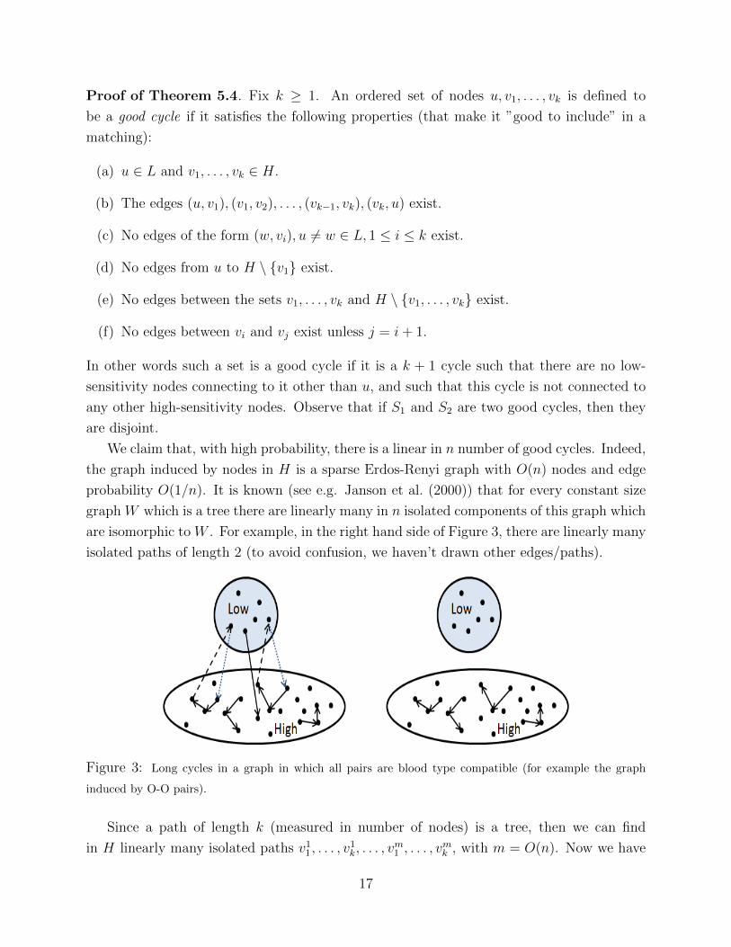
Proof of Theorem 5.4. Fix k ≥ 1. An ordered set of nodes u, v1, . . . , vk is defined to

be a good cycle if it satisfies the following properties (that make it ”good to include” in a

matching):

(a) u ∈ L and v1, . . . , vk ∈ H.

(b) The edges (u, v1), (v1, v2), . . . , (vk−1, vk), (vk, u) exist.

(c) No edges of the form (w, vi), u 6= w ∈ L, 1 ≤ i ≤ k exist.

(d) No edges from u to H \ {v1} exist.

(e) No edges between the sets v1, . . . , vk and H \ {v1, . . . , vk} exist.

(f) No edges between vi and vj exist unless j = i+ 1.

In other words such a set is a good cycle if it is a k + 1 cycle such that there are no low-

sensitivity nodes connecting to it other than u, and such that this cycle is not connected to

any other high-sensitivity nodes. Observe that if S1 and S2 are two good cycles, then they

are disjoint.

We claim that, with high probability, there is a linear in n number of good cycles. Indeed,

the graph induced by nodes in H is a sparse Erdos-Renyi graph with O(n) nodes and edge

probability O(1/n). It is known (see e.g. Janson et al. (2000)) that for every constant size

graph W which is a tree there are linearly many in n isolated components of this graph which

are isomorphic to W . For example, in the right hand side of Figure 3, there are linearly many

isolated paths of length 2 (to avoid confusion, we haven’t drawn other edges/paths).

Figure 3: Long cycles in a graph in which all pairs are blood type compatible (for example the graph

induced by O-O pairs).

Since a path of length k (measured in number of nodes) is a tree, then we can find

in H linearly many isolated paths v11, . . . , v

1k, . . . , v

m1 , . . . , v

mk , with m = O(n). Now we have

17

established before that we can construct a linear size matching from L into the set v11, . . . , v

m1 .

The sources of these matchings are denoted by u1, . . . , um. Finally, since the probability of

an edge (vlk, ul) is pL which is a constant, then for a linear fraction of these sets such an

edge exists (these are the dashed edges to L nodes in the left side of Figure 3). Thus there

is a constant fraction of m (and therefore of n) paths ul, vl1, . . . , vlk which are also cycles by

connecting vlk to ul. We have established an existence with high probability of disjoint k+ 1

cycles Sl = ul, vl1, . . . , vlk, 1 ≤ l ≤ r, for some r = O(n). This proves the claim.

Now consider any optimal cycle cover Wk achieving Wk with cycles up to length k. We

will use Wk and k + 1 cycles Sl = ul, vl1, . . . , vlk, 1 ≤ l ≤ r in order to build a cycle cover

with cycles of length ≤ k + 1 which is larger than Wk by a linear additive term. Observe

first that for every l = 1, . . . , r, nodes vl2, . . . , vlk cannot be part of Wk, since the shortest

(and the only) cycle they belong to is ul, vl1, . . . , vlk which has length k + 1. On the other

hand both ul and vl1 can belong to Wk. Observe, however, that if they do, they must belong

to the same cycle since there are no L nodes pointing to vl1 other than ul. Now every cycle

Sl = ul, vl1, . . . , vlk which is disjoint from Wk we simply add to Wk, and for every cycle Sl

which intersects with some cycle C via nodes ul, vl1, we delete C from Wk and add to it Sl

to Wk. In the first case, the number of nodes covered increases by k+ 1. In the second case

it increases by at least (k + 1) − k = 1, since ul and vl1 belonged to a cycle with length at

most k as a part of Wk. Then the total number of nodes thus covered is at least r = O(n).

This implies Wk+1 −Wk ≥ r = O(n) with high probability and the proof of the theorem is

complete.

5.2 Not too dense, not too sparse (ε > 0)

In the next two theorems we analyze the benefit from increasing the maximum chain length

in the graph D(n, λ, t(n), p, cn−1+ε) where ε > 0 for different number of non-directed donors

in the graph. The first result considers a linear fraction of non-directed donors.

Theorem 5.6. Fix k ≥ 2 and l ≥ k and let t(n) = βn ,β > 0,λ > 0 and ε < 1k.

1. Relatively few non-directed donors and low-sensitized patients: Suppose β + λ < 1−λl+1

.

With probability approaching one Wk,l+1 = Wk,l + ρn + o(n) for some ρ > 0. In this

case, in every (k, l + 1)-efficient allocation every L node is in a k length cycle with

k − 1 H nodes, and every NDD initiates a chain of length l + 1 of only H nodes.

2. Many non-directed donors: If β > 1−λl

then Wk,l = n, i.e. chains of length l are

sufficient to cover all nodes. If λ > 1k, cycles of length k are sufficient to cover all

nodes.

18

3. Every (k, l)-efficient allocation matches all (but at most 1 if k = 2) L nodes.

Similar arguments to the proof of the first part of Theorem 5.6 can also show that if

1 > λ > 0, with probability approaching one Wk+1,l matches linearly more nodes than Wk,l

(even if ε < 1k+1

). The cases between the first and second parts of Theorem 5.6 can also be

analyzed. The main point, however, is that if there is an allocation that matches every L

node and every NDD node in exchanges that involve only H nodes, and there is still a linear

fraction of H nodes remaining, then extending the chain length (or cycle length) increases

the size of the allocation linearly.

In the next theorem we show that even when there is a very small number of non-directed

donors, moving from bounded chains to unbounded chains linearly increases the size of the

allocation.

Theorem 5.7. (Limited supply of non-directed donors): Fix k ≥ 2 and l ≥ k and let

t(n) = z for some bounded integer z ≥ 1 and ε < 1k.

1. Few low-sensitized patients: If 0 < λ < 1k+1

, with probability approaching one Wk,∞ =

Wk,l + ρn+ o(n).

2. Many low-sensitized patients: If λ > 1k, cycles of length k are sufficient to cover all

nodes.

The proofs of Theorems 5.6 and 5.7 use the result of the next lemma that shows that the

number of disjoint cycles consisting of only H nodes of size k is relatively small. The lemma

is of independent interest, and characterizes the need for longer cycles when all nodes in the

graph are H nodes.

Lemma 5.8. (All H nodes): Suppose t(n) = 0 and λ = 0 and let D = D(n, 0, 0, p, cn−1+ε).

1. If 0 < ε < 1k, Wk = Θ(nkε) in almost every D. Furthermore the size of the k-efficient

allocation is Θ(nkε).24

2. If ε < 0, Wk = o(1) in almost every D.

3. If ε > 1k, Wk = n in almost every D.

24For two functions f(n) and g(n) we write f = Θ(g) if there exist constants c1 < c2 such that c1g(n) ≤f(n) ≤ c2g(n) for every sufficiently large n.

19

The idea of the proof is to show that in sparse enough graphs the number of cycles of

size exactly k + 1 in the pool is approximately the number of disjoint cycles of size k + 1.

Moreover the number of cycles of size at most k is smaller than the number of cycles of size

k + 1. We can now sketch the proof of Theorem 5.6.

Sketch of Proof of Theorem 5.6.

We begin with the first part (the second part is similar). For simplicity assume here there

no L nodes (the case with L nodes is slightly more delicate; see the appendix for the full

proof). Suppose that β < 1l+1

as in part 1. Then there exists l+ 1 disjoint sets, H1, . . . , Hl+1

each containing only H nodes and each of equal size βn (we neglect here that βn may not

be an integer).

By the Erdos Renyi theorem for bipartite graphs, for each i, there is a perfect (one-way)

matching from Hi to Hi+1. Similarly there is a perfect one-way matching from the set of

NDDs to H1. Note that this creates βn disjoint paths each beginning from an NDD donor.

Finally, by Lemma 5.8, the size of the maximum allocation using cycles of length k or less

and chains of size l or less in the graph induced only by H nodes is sublinear in n. Therefore,

it must be that the l + 1 length chains we constructed must increase the efficient allocation

by a linear fraction. Finally the third part follows since either all L nodes have been used

in the construction, or in the graph induced by the remaining L nodes there is an allocation

that matches all pairs but at most 1 using 2-way cycles (by the Erdos-Renyi Theorem).

To summarize, there are density thresholds that determine the need for long chains and

cycles to obtain efficiency. When the graph is sparse, even one non-directed donor can make

a difference, even in patient pools of practical size, as shown in Table 2.

6 Simulations

6.1 Simulated data

In this section we consider simulated data to further demonstrate the effectiveness of chains

and show that our model and results provide a good approximation for the graphs we observe

in practice. In all our simulations we measure the effectiveness of longer cycles and longer

chains. In each scenario we ran 300 trials.

Our first set of simulations are done on simulated pairs in which patients and donors

have the same blood type, varying between 40 to 100 nodes. The graphs are created as

follows. Each node is randomly chosen to be an H node with probability 0.73 and an L

node otherwise. An incoming edge from each donor to an L node is generated with pL =

0.45. We let pH(n) = 0.03 which is consistent with the likelihood given in Table 4 for high

PRA patients in the A-A pool. (Sensitivity analysis with pH(n) = 0.05, corresponding to the

20

average high PRA of 0.95 we see in the O-O pairs, produced very similar qualitative results).

For pools of size up to 150 the pH matching probabilities can be viewed as significantly belowlnnn

which is the Erdos-Renyi threshold for perfect matching.

Figures 4a and 4b describe the average number of H and L matched nodes, allowing

for different maximum cycle and chain length. Observe the additional high PRA matches

achieved from increasing the maximum cycle and chain lengths. Moreover, observe that the

number of low PRA matched nodes is almost a constant, confirming that almost the entire

benefit from using longer chains goes to high PRA patients.

(a) 80 nodes. (b) 100 nodes.

Figure 4: Number of matches and high PRA matches (y-axis) obtained for different maximum cycle and

chain lengths (the x-axis indicates the type of efficient allocation). The percentage of L nodes is 0.27 and

the probability for an H node to have an incoming link from any given node is set to pH = 0.03. Note that

low PRA patients are not harmed by the increase in cycle and chain length, while the benefits go almost

entirely to high PRA patients. (Note that all the low PRA lines almost completely overlap.)

In Table 5 we present similar results for patient pools of various sizes. Again, observe

the significant number of additional matches from increasing cycle/chain size, and note that

almost all L pairs are always matched, so that the entire benefit goes to highly sensitized

patients.

6.2 Simulations using clinical data

In this section we provide further experimental results using clinical data instead of simulated

data. In each trial, pairs are drawn from the historical data set with resampling. Table 6

reports results similar to those in the figures in the previous section. Observe the substantial

number of additional matches from increasing cycle/chain size, and that almost all the benefit

goes to highly sensitized patients. To make the sample size as big as possible, we used both

O-O and A-O pairs (note that in this pool all pairs are blood type compatible).

21

Size NDDs (2, 3) (3, 3) (3, 4) (3,∞) (∞,∞)

40 (29.5) 0 11.5 (2.67) 15.83 (5.69) 15.83 (5.69) 15.83 (5.69) 18.62 (8.16)

1 13.17 (3.29) 16.79 (5.78) 16.94 (5.95) 17.75 (6.7) 19.14 (8.02)

5 16.4 (6.23) 18.57 (8.05) 19.17 (8.64) 20.09 (9.53) 20.37 (9.8)

60 (43.65) 0 21.05 (6.04) 29.1 (12.84) 29.1 (12.84) 29.1 (12.84) 36.61 (20.26)

1 21.76 (6.62) 29.68 (13.43) 29.93 (13.7) 32.7 (16.44) 36.19 (19.89)

5 25.72 (10.31) 31.75 (15.87) 32.9 (17.05) 37.57 (21.67) 37.8 (21.89)

80 (58.48) 0 29.81 (9.49) 43.4 (21.9) 43.4 (21.9) 43.4 (21.9) 57.52 (36)

1 31.54 (10.94) 44.45 (22.87) 44.79 (23.2) 50.4 (28.8) 58.72 (37.09)

5 36.1 (15.16) 46.9 (25.54) 48.4 (27.04) 58 (36.61) 58.62 (37.22)

100 (73.36) 0 40.09 (14.49) 59.3 (32.69) 59.3 (32.69) 59.3 (32.69) 81.26 (54.61)

1 41.98 (16.09) 60.91 (34.15) 61.28 (34.51) 70.21 (43.45) 82.28 (55.49)

5 47.05 (20.32) 64.1 (36.97) 65.71 (38.59) 81.36 (54.23) 83.18 (56.04)

Table 5: Average size of the (k, l)-efficient allocations (cycles up to length k and chains up to length l)

with different number of non-directed donors (NDDs) and different size pools with pairs that all have the

same blood type. The number of matched high PRA patients is given in parenthesis. pH is set to 0.03.

Finally, Table 7 provides similar experimental results, only sampling is done from the

entire exchange pool rather than just sampling A-O and O-O pairs.

Observe that long chains allow more than 10% more transplants than when chains are

limited to length 3 when the pool size is more than 50. Note that the additional high

PRA patients who can be matched often substantially exceeds 10%. Finally, allowing for

unbounded chains and 3-way cycles obtains almost the same number of matches that can be

achieved when both cycles and chains can be unbounded in size, so long chains substitute

well for large cycles when there are some non-directed donors available.25

7 Conclusion

There are a number of ways in which barter may be inefficient. Jevons (1876) famously

pointed to the double coincidences needed for pairwise exchange. For kidney exchange,

theory based on large graphs that become very densely connected in the limit predicts that

also allowing 3-way cycles and short chains will overcome this difficulty as the number of

patients enrolled in exchange pools becomes large.

However the compatibility graphs so far seen in practice are sparse. We show here

empirically that long (non-simultaneous) chains are needed for efficiency due to the sparsity

25Dickerson et al. (2012) also examine simulated data and show that long chains are beneficial, in smaller

pools than ours. They consider smaller pools due to computational complexity issues.

22

Size NDDs (2, 3) (3, 3) (3, 4) (3,∞) (∞,∞)

40 (28.25) 0 10.63 (3.63) 15.71 (6.17) 15.71 (6.17) 15.71 (6.17) 18.63 (8.25)

1 12.04 (4.04) 16.24 (6.29) 16.5 (6.48) 17.76 (7.41) 18.71 (8.1)

5 16.5 (6.63) 18.86 (8.01) 19.54 (8.63) 20.54 (9.36) 20.61 (9.39)

60 (42.64) 0 18.18 (6.65) 26.3 (11.37) 26.3 (11.37) 26.3 (11.37) 30.64 (14.78)

1 20 (7.42) 27.4 (11.74) 27.68 (11.97) 29.86 (13.83) 31.23 (14.91)

5 24.82 (10.07) 29.87 (13.51) 30.72 (14.27) 32.73 (15.99) 32.81 (16.08)

80 (56.89) 0 26.89 (10.22) 38.8 (17.7) 38.8 (17.7) 38.8 (17.7) 43.82 (22.17)

1 28.05 (10.84) 38.57 (17.46) 38.84 (17.69) 41.9 (20.45) 43.89 (22.22)

5 34.81 (14.57) 43.05 (20.37) 44.25 (21.46) 46.68 (23.7) 46.73 (23.78)

100 (70.67) 0 35.26 (13.63) 50.3 (23.35) 50.3 (23.35) 50.3 (23.35) 56.56 (29.14)

1 35.86 (13.82) 50.35 (23.32) 50.72 (23.65) 54.28 (27) 56.38 (29.01)

5 43.39 (18.01) 54.31 (26.05) 55.51 (27.2) 58.91 (30.34) 58.98 (30.42)

Table 6: Average number of matched patients through (k, l)-efficient allocations (cycles up to length k

and chains up to length l) with different numbers of non-directed donors (NDDs) and different size pools.

Pairs are all blood type compatible, drawn from the O-O and A-O pairs. The number of matched high PRA

patients is given in parenthesis.

of compatibility graphs that arise when many patients are very highly sensitized. We further

provide theoretical foundations to better understand the structure of efficient allocations in

sparse compatability graphs.

We show empirically, theoretically, and by simulation that highly sensitized patients are

the ones who benefit from long chains.26 Moreover, this benefit for highly sensitized patients

does not harm low-sensitized patients. Our findings suggest that tissue type incompatibilities

together with medium pool sizes are of first order importance in understanding efficient

kidney exchange, and that as long as we see such a high percentage of highly sensitized

patients, long chains will help achieve more transplants, and each non-directed donor can

have a big effect.

Our results show that even in hindsight (after some reasonable number of pairs arrive

to the system), long chains are very effective. An important issue for future research is to

understand how to choose allocations dynamically, since these pairs may arrive at different

times.

26This threefold approach allows each of the three legs to be tested by the others. The theoretical model

concerns infinitely large graphs that remain sparse and obtains analytical results that explain (in very large

graphs) the need for long chains. The simulations show that the random-graph model and the analytical

results for infinite graphs apply to patient-donor pools of the size seen in practice, and the empirical results

show that the actually observed patient-donor population yields results that correspond to the theoretical

and simulation models.

23

Size NDDs (2, 3) (3, 3) (3, 4) (3,∞) (∞,∞)

40 (20.8) 0 6.03 (1.34) 8.14 (2.15) 8.14 (2.15) 8.14 (2.15) 9.45 (2.79)

1 7.7 (1.71) 9.67 (2.42) 9.94 (2.5) 10.88 (2.9) 11.23 (3.05)

5 13.2 (3.1) 14.25 (3.5) 14.64 (3.66) 15.09 (3.86) 15.09 (3.86)

80 (42.37) 0 15.14 (4.2) 21.65 (7.14) 21.65 (7.14) 21.65 (7.14) 25.98 (9.45)

1 17.4 (4.72) 23.6 (7.5) 23.99 (7.66) 27.18 (9.3) 27.67 (9.63)

5 24.65 (6.5) 29.12 (8.54) 30.23 (9.11) 32 (10.2) 32.02 (10.28)

120 (62.95) 0 26.1 (7.5) 37.7 (13.25) 37.7 (13.25) 37.7 (13.25) 44.65 (17.5)

1 27.77 (7.61) 39.1 (13.04) 39.61 (13.1) 45.27 (16.7) 45.75 (17.08)

5 36.56 (10.33) 46.34 (15.19) 48.02 (16.04) 51.38 (18.34) 51.39 (18.44)

160 (83.79) 0 37.06 (11.11) 53.78 (19.35) 53.78 (19.35) 53.78 (19.35) 62.55 (25.04)

1 39.76 (11.57) 56.24 (20.1) 56.78 (20.4) 62.34 (23.89) 65.15 (26.08)

5 48.44 (14.06) 63.71 (22.22) 65.62 (23.39) 71.22 (27.16) 71.22 (27.47)

200 (103.55) 0 48.94 (14.76) 71.79 (26.37) 71.79 (26.37) 71.79 (26.37) 82.82 (34.15)

1 51.22 (14.89) 73.52 (26.99) 74 (27.28) 79.05 (30.62) 84.42 (34.5)

5 58.99 (17.37) 79.42 (29) 81.64 (30.22) 89.37 (35.55) 89.4 (36)

Table 7: Average number of matched patients using (k, l)-efficient allocations (cycles up to length k and

chains up to length l) with different numbers of non-directed donors (NDDs) and different size pools. Pairs

are all blood type compatible, drawn from the entire dataset of such pairs of all blood types. The number

of matched high PRA patients is given in parenthesis.

One of the key tasks of market design is to establish a thick market (cf. Roth (2008)).

Thickness in the kidney exchange marketplace is determined by the number of pairs and the

number of non-directed donors, but also by the density of the compatibilities between donors

and patients of different pairs. We have seen here that when the market is not too thick,

the capacity to implement longer cycles and chains plays an important role in efficiency.

This observation seems likely to generalize well beyond the particular case of kidney

exchange, a market in which prices are outlawed, to other markets that are cash or credit

constrained.

Consider for example the market for residential real estate in the United States. It is not

uncommon for purchase and sales agreements to have contingency clauses saying that the

purchase of a house is contingent on the buyer’s successful sale of his own home in time to

close the deal. Thus a given sale may go through only if it is part of a chain of sales that may

begin with a non-contingent buyer (e.g. a buyer who does not have a home that he must

sell before he can buy another). Such a non-contingent buyer plays much the same role as a

non-directed donor here. Similarly, bridge loans that allow a purchase to go through before

the buyer has sold his own home allow for such chains to be non-simultaneous.

In conclusion, an obstacle to bilateral barter is the need to find double coincidences of

24

wants. Developing the capability to arrange trades in longer cycles and chains helps overcome

this barrier, in markets like kidney exchange in which money and prices are not available to

clear the market, and very likely in other markets as well, in which credit and cash constraints

prevent prices from completely clearing the market. In the case of kidney exchange, long

non-simultaneous chains of the sort proposed in Roth et al. (2006) are proving increasingly

important, and the present paper offers some new insight into why this is the case.

References

D. J. Abraham, A. Blum, and T. Sandholm. Clearing Algorithms for Barter Exchange

Markets: Enabling Nationwide Kidney Exchanges. In Proc of the 8th ACM Conference

on Electronic commerce (EC), pages 295–304, 2007.

I. Ashlagi and A. E. Roth. Free riding and participation in large scale, multi-hospital kidney

exchange. NBER paper no. w16720, 2011.

I. Ashlagi and A.E. Roth. New Challenges in Multi-hospital Kidney Exchange. American

Economic Review Papers and Proceedings, 2012. Forthcoming.

I. Ashlagi, F. Fischer, I. Kash, and A.D. Procaccia. Mix and Match. In Proc of the 11th

ACM Conference on Electronic Commerce, pages 295–304, 2010.

I. Ashlagi, D. S. Gilchrist, A. E. Roth, and M. A. Rees. Nonsimultaneous Chains and

Dominos in Kidney Paired Donation - Revisited. American Journal of Transplantation,

11:984–994, 2011a.

I. Ashlagi, D. S. Gilchrist, A. E. Roth, and M. A. Rees. NEAD Chains in Transplantation.

American Journal of Transplantation, 11:2780–2781, 2011b.

L. M. Ausubel and T. Morrill. Sequential Kidney Exchange. Working paper, NC State

University, 2010.

T. Bohman and A. Frieze. Karp-sipser on random graphs with a fixed degree sequence.

Combinatorics, Probability and Computing, 20(5):721–741, 2011.

J. P. Dickerson, A. D. Procaccia, and T. Sandholm. Optimizing Kidney Exchange with

Transplant Chains: Theory and Reality. Proc of the eleventh international conference on

autonomous agents and multiagent systems, 2012.

25

S. E. Gentry, R. A. Montgomery, B. J. Swihart, and D. L. Segev. The Roles of Dominos and

Nonsimultaneous Chains in Kidney Paired Donation. American Journal of Transplanta-

tion, 9:1330–1336, 2009.

S.E. Gentry and D.L. Segev. The honeymoon phase and studies of nonsimultaneous chains

in kidney paired donation. American Journal of Transplantation, 11:2778–2779, 2011.

S. Janson, T. Luczak, and R. Rucinski. Random Graphs. A John Wiley & Sons, 2000.

W. S. Jevons. Money and the Mechanism of Exchange. New York: D. Appleton and Com-

pany., 1876. http://www.econlib.org/library/ YPDBooks/Jevons/jvnMME.html.

M. Krivelevich, E. Lubetzky, and B. Sudakov. Longest cycles in sparse random digraphs.

Random Structures and Algorithms, 2012. Forthcoming.

D. F. Manlove and G. O’Malley. Paired and Altruistic Kidney Donation in the UK: Algo-

rithms and Experimentation. In Proc of the 11th International Symposioum of Experi-

mantal Algorithms, 2012.

M. A. Rees, J. E. Kopke, R. P. Pelletier, D. L. Segev, M. E. Rutter, A. J. Fabrega, J. Rogers,

O. G. Pankewycz, J. Hiller, A. E. Roth, T. Sandholm, M. U. Unver, and R. A. Montgomery.

A non-simultaneous extended altruistic donor chain. New England Journal of Medecine,

360:1096–1101, 2009.

A. E. Roth. What have we learned from market design? Economic Journal, 118:285–310,

2008.

A. E. Roth, T. Sonmez, and M. U. Unver. Kidney exchange. Quarterly Journal of Economics,

119:457–488, 2004.

A. E. Roth, T. Sonmez, and M. U. Unver. A kidney exchange clearinghouse in New England.

American Economic Review Papers and Proceedings, 95(2):376–380, 2005.

A. E. Roth, T. Sonmez, M. U. Unver, F. L. Delmonico, and S. L. Saidman. Utilizing list

exchange and nondirected donation through chain kidney paired donations. American

Journal of Transplantation, 6:2694–2705, 2006.

A. E. Roth, T. Sonmez, and M. U. Unver. Efficient kidney exchange: coincidence of wants in

markets with compatibility-based preferences. American Economic Review, 97:828–851,

2007.

26

S. L. Saidman, A. E. Roth, T. Sonmez, M. U. Unver, and F. L. Delmonico. Increasing the

Opportunity of Live Kidney Donation by Matching for Two and Three Way Exchanges.

Transplantation, 81:773–782, 2006.

T. Sonmez and M. U. Unver. Altruistic Kidney Exchange. Working paper, 2011.

P. Toulis and D. C. Parkes. A Random Graph Model of Kidney Exchanges : Optimality and

Incentives. In Proc of the 11th ACM Conference on Electronic Commerce, pages 323–332,

2011.

M. U. Unver. Dynamic Kidney Exchange. Review of Economic Studies, 77(1):372–414, 2010.

8 Appendix

To prove Theorem 5.3 we need Theorem 5.4 which its proof makes use of Lemma 5.5.

Proof of Lemma 5.5. The existence and the actual value of the limit α(µ, c) can be es-

tablished using the Karp-Sipser algorithm technique (see Bohman and Frieze (2011)).

Since each side contains a linear number of isolated nodes, then α(µ, c) < min(µ, 1− µ).

Similarly, there exists a linear set of isolated edges, and thus α(µ, c) > 0. To prove strict

monotonicity, fix c < c′ and consider graphs G(n, µ, c/n) and G(n, µ, c′/n) coupled on the

same probability space by adding edges to G(n, µ, c/n) with probability x such that c/n +

(1− c/n)x = c′/n. The newly obtained graph is exactly G(n, µ, c′/n). Since the extra edges

create a linear size matching between isolated nodes in G(n, µ, c/n), we see that M(n, µ, c′/n)

is larger than M(n, µ, c/n) by a linear term and the proof is complete.

Proof of Theorem 5.3. Let d1, . . . , dz be the set of non-directed donors and let m =

max(k, l). Define H1 be the set of nodes u in H such that there is at least one link from

L∪{d2, . . . , dz} to u. Namely, it is the set of nodes reachable from L pairs and non-directed

donors other than d1. The reason for excluding d1 will become clear shortly. Assuming Hi−1

is defined, let Hi be the set of nodes u in H \H1 ∪ · · · ∪Hi−1 such that there exists at least

one node in Hi−1 which connects to u. Consider the graph H \H1∪ · · · ∪Hm−1. None of the

nodes in this graph can participate in a (k, l)-efficient allocation unless d1 is used, since they

all have distance at least m from L pairs and non-directed donors d2, . . . , dz (it is well-known

that there are no cycles of constant size in the graph induced by only H nodes). Now when

we include d1 into the optimal allocation, it can increase it most by l as this is an upper

bound chain lengths.

We claim that for large enough c, the set H \ H1 ∪ · · · ∪ Hm−1 contains a linear length

directed path v1, . . . , vγn for some constant γ > 0. First let us show how this implies the

27

result. With probability (1 − c/n)γn/2 ≈ exp(−cγ/2) = O(1), the non-directed donor d1

connects to one of the nodes v1, . . . , vγn/2. This computation is valid since the definition

of Hi, 1 ≤ i ≤ m did not reveal any information about the links from d1. In this case we

have obtained a linear size (≥ γn/2) chain originating from the non-directed donor d1 and

therefore Wk,∞ ≥ Wk,l − l + γn/2 and the proof is complete.

To prove the claim, note that the expected size of H \H1 is

E[|H \H1|] = |H|(1− c/n)|L|+z−1

= |H|(1− c/n)λn+z−1

= n(1− λ) exp(−λc− o(1))

= nρ1(1− o(1)),

where we have use notation ρ1 = (1−λ) exp(−λc). Using standard concentration results, we

have that in factH1 = E[H1](1+o(1)) with high probability, implying |H\H1| = nρ1(1−o(1)).

Similarly, with high probability

|H \ (H1 ∪H2)| = |H \H1|(1− c/n)|H1|(1− o(1))

= nρ1 exp(−c(1− ρ1))(1− o(1))

= nρ2(1− o(1)),

with ρ2 defined as ρ1 exp(−c(1−ρ1)). This also gives |H2| = (ρ1−ρ2)n(1−o(1)). Continuing

till m, we conclude that with high probability

|H \ ∪i≤m−1Hi| = ρm−1n(1− o(1)),

where ρi is defined recursively as ρi−1 exp(−c(ρi−2 − ρi−1)) and ρ0 = 1. Now, observe that

ρ1 converges to unity as λ→ 0. By induction in i = 1, 2, . . . ,m− 1 we obtain that the same

applies to ρm−1. Thus by taking λ sufficiently small, we have ρm−1 ≥ 1/2. In conclusion,

the set H \H1 ∪ · · · ∪Hm−1 contains at least n/2 with high probability when constant λ is

sufficiently small. For every two nodes u and v in this set, the probability of an edge is still

c/n, independently for all edges, since we have not revealed any information about the edges

within this set. By a recent theorem by Krivelevich et al. (2012), there exists a directed path

with a linear length in this graph. (In fact their theorem proves that this length approaches

the size of the entire set, namely n/2, as c increases). This concludes the proof.

Proof of Lemma 5.8. Let D be a directed random graph with n nodes and edge probabil-

ity q = cn−1+ε where ε < 1k. Denote by Sk the total number of k-way cycles (not necessarily

disjoint) in the directed random graph D. Observe that

ESk =

(n

k

)qk = Θ((nq)k) = Θ

(nkε), (1)

28

where the first equality follows since k is a constant. Furthermore, since k is a constant

E

(k∑l=2

Sl

)= Θ

(nkε). (2)

Suppose 0 < ε < 1k. By (1) ESl = o(ESk) for any 2 ≤ l ≤ k − 1. Therefore to prove the

first part it is sufficient to show that the number of disjoint cycles of size k is approximately

the same number as the number of cycles of size k and that the number of cycles of size k

is concentrated around its mean.

Denote by Qk the size of the maximum allocation containing only k-way cycles (note

that this is different than Wk which also allows cycles shorter than k). We show first that

EQk = Θ(ESk).

Let Yk be the number of k-way cycles that each intersects another k-way cycle. Note

that Qk ≥ Sk − Yk. First we show that EYk = o(ESk) = o(nkε). Observe that two different

k-way cycles in the graph overlap if and only if there exist l, 0 ≤ l ≤ k − 2, such that they

have l edges in common and together they have 2k − l − 1 nodes. Therefore

EYk = Θ(k−2∑l=0

(n

2k − l − 1

)q2k−l) = Θ

(k−2∑l=0

n2k−l−1q2k−l

)=

2k−l−1∑l=0

n−1+2kε−lε = Θ(n−1+2kε

)= o

(nkε), (3)

where second equality follows since k is a constant, and since ε < 1k, −1 + 2kε < kε implying

the last inequality.

It remains to show that Yk and Sk are both concentrated around their means. Let

0 < δ < 1− kε. By Markov’s inequality

Pr(Yk ≥ n−1+2kε+δ

)≤ n−1+2kε

n−1+2kε+δ(4)

which tends to zero by the assumption on δ. Therefore by (4), Yk = o(ESk).

To show that Sk is concentrated around its mean we calculate its variance and apply

Chevyshev’s inequality. A set of k nodes and an order over them define a random variable

which takes the value 1 if these nodes contain a cycle in the given order and zero otherwise.

The covariance between any two such random variables is 0 unless they have 1 ≤ l ≤ k − 2

edges in common. Therefore

V ar(Sk) ≤ Θ(2k−l−1∑l=1

2

(n

2k − l − 1

)q2k−l) = Θ(2

2k−l−1∑l=1

n−1+2kε−lε) = Θ(n(2k−1)ε−1).

29

Applying Chevyshev’s inequality for small enough δ > 0

Pr(|Sk − ESk| ≥ nkε−δ

)≤ Θ(

2n(2k−1)ε−1)

n2kε−2δ), (5)

implying that Sk = O(ESk) and therefore Yk = o (Sk).

The second part follows by (2) and similar analysis.

Proof of Theorem 5.6. We begin with the first part. Let Rk,l be the size of the efficient

allocation with cycles of size at most k such that each cycle contains at least one L node,

and chains of length at most l. By Lemma 5.8 the size of the k-efficient allocation in the

graph induced only by H nodes is Θ(nkε), i.e. sublinear in the size of the graph. Therefore it

sufficient to show that Rk,l+1 = Rk,l + ρn+ o(n) for some ρ > 0. To prove this we show that

with high probability there exists an allocation that each L node is part of a k-way cycle

with k − 1 H nodes, and each NDD begins a chain of size l that contains only H nodes.

To avoid some minor subtleties we assume that βn and λn are integers. Let H1, . . . , Hl+k

be a collection of disjoint subsets of H nodes such that |Hi| = βn for every 1 ≤ i ≤ l + 1

and |Hi| = λn for every l + 2 ≤ i ≤ l + k. Too that such a partition exists not that

βn(l + 1) + λnk < βn(l + 1) + λn(l + 1) < (1− λ)n where the first inequality follows since

k ≤ l and the second inequality follows since β + λ < 1−λl+1

.

Let Bi,i+1 be the bipartite graph in which one side of the graph consist of the nodes in

Hi and the other side consists of the nodes in Hi+1 and there is an edge from v to w if

and only if v ∈ Hi, w ∈ Hi+1 and (v, w) is an edge in the compatibility graph. For every

1 ≤ i ≤ l, B(i, i + 1) is a bipartite random graph with edge probability q(n) = cn−1+ε.

Therefore, since q(n) >> ( lognn

), by Erdos-Renyi Theorem for every i, such that 1 ≤ i ≤ l

there exists a perfect matching in B(i, i + 1). In addition there exist a perfect matching

in the graph induced by the set of NDDs and H0. Since l is finite we obtained that with

probability approaching one there are βn disjoint chains each of length l + 1.

Next we construct k-way cycles using the H nodes in the sets Hl+2, . . . , Hl+k and the set

of L nodes. By similar arguments as above, for every l + 2 ≤ i ≤ l + k with probability

converging to one there exist a perfect matching in B(i, i + 1). Thus with high probability

there are λn disjoint paths each of length k− 1 using the H nodes in Hl+2, . . . , Hl+k. Denote

this set of paths by Q. We next show that with high probability one can extend each of

these paths to a cycle of length k adding one distinct L node.

Consider the following bipartite graph G. One side of the graph consists of the L nodes,

and the other side consists of λn nodes each representing a path in Q and denoted by v(σ)

where σ ∈ Q. There is an edge in G from w ∈ L and v(σ) for some σ ∈ Q if and only if there

exists an edge from w to the first node of σ and there exists an edge from the last node of σ

to w in the compatibility graph. Since each such edge exist with probability pq(n) >> lognn

,

30

by the Erdos-Renyi theorem, we obtain that almost every such graph G contains a perfect

matching. Again, since k and l are both finite, we obtained the desired allocation with high

probability, completing the first part of the proof.

The second part follows from a similar construction of paths, and since all L nodes (but

at most one) can be matched to each other using 2-way cycles, the third part follows.

Proof of Theorem 5.7. By Lemma 5.8 there is sublinear number of cycles of size at most

k + 1 in the graph induced only by H nodes. Consider the graph G induced by all H nodes

that are not part of k + 1 cycle. Since G is of linear size, there is a cycle of linear size in a

directed random graph with edge probability at least cn

for any constant c ≥ 1. Let C be

such a cycle.

The probability that a non-directed donor does not have an edge to any of the nodes in

C is (1− n−1+ε)Θ(n) which approaches zero as n tends to infinity. Therefore a non-directed

donor can initiate a linear sized chain.

The second part follows from Lemma 5.8.

31