the nature of statistics - auburn...
TRANSCRIPT

Copyright © 2016, 2012, 2008 Pearson Education, Inc. Chapter 1, Slide 1
Chapter 1The Nature of
Statistics
Copyright © 2016, 2012, 2008 Pearson Education, Inc. Chapter 1, Slide 1
Copyright © 2016, 2012, 2008 Pearson Education, Inc. Chapter 1, Slide 2
First Week Coverage:
Section 1.1: Statistics Basics
Section 2.1: Variables and Data
Section 2.2: Organizing Qualitative Data
Section 2.3: Organizing Quantitative Data
Section 2.4: Distribution Shapes
STAT 2510, Section 130
Wed/Fri, Aug. 17/19

Copyright © 2016, 2012, 2008 Pearson Education, Inc. Chapter 1, Slide 3
Section 1.1
Statistics Basics

Copyright © 2016, 2012, 2008 Pearson Education, Inc. Chapter 1, Slide 4
Copyright © 2012, 2008, 2005 Pearson
Education, Inc.
Definition 1.1
Descriptive statistics includes the construction of
graphs, charts, and tables and the calculation of
various descriptive measures such as averages,
measures of variation, and percentiles.
Descriptive Statistics
Descriptive Statistics consists of methods for organizing
and summarizing information.
Descriptive statistics describe samples

Copyright © 2016, 2012, 2008 Pearson Education, Inc. Chapter 1, Slide 5
Example 1.1
The 1948 Baseball Season. In 1948, the Washington
Senators played 153 games, winning 56 and losing
97. They finished seventh in the American League
and were led in hitting by Bud Stewart, whose
batting average was .279.
The work of baseball statisticians is an illustration of
descriptive statistics.

Copyright © 2016, 2012, 2008 Pearson Education, Inc. Chapter 1, Slide 6
Example 1.1.b
This section of STAT 2510 is a sample from all
sections of STAT 2510 students Fall 2016
(population). Here are a few descriptive statistics,
Sample size: n = 95, students registered in class
Gender: 32 Males (33.7%) and 63 Females
(66.3%)
Colleges: Mode: 33.7% of students are in Nursing
Class: Mode: 53.7% of students are Sophomores

Copyright © 2016, 2012, 2008 Pearson Education, Inc. Chapter 1, Slide 7
Definition 1.2
Population and Sample
Population: The collection of all individuals or items under
consideration in a statistical study.
Sample: That part of the population from which information
is obtained.
Parameters are numerical values describing a population
Statistics are numerical values describing a sample.

Copyright © 2016, 2012, 2008 Pearson Education, Inc. Chapter 1, Slide 8
Example 1.2
Political polling provides an example of inferential
statistics. Interviewing everyone of voting age in the
United States on their voting preferences would be
expensive and unrealistic. Statisticians who want to
gauge the sentiment of the entire population of U.S.
voters can afford to interview only a carefully chosen
group of a few thousand voters. This group is called
a sample of the population.

Copyright © 2016, 2012, 2008 Pearson Education, Inc. Chapter 1, Slide 9
Example 1.2.b
There are a total of 11 sections of STAT 2510 for a
total population of size N=624 students. The
various sample sizes are n1 = 27, n2 = 48, n3 = 26,
n4 = 95, n5 = 27, n6 = 132, n7 = 27, n8 = 93, n9 = 95,
n10 = 27, and n11 = 27.

Copyright © 2016, 2012, 2008 Pearson Education, Inc. Chapter 1, Slide 10
Copyright © 2012, 2008, 2005 Pearson
Education, Inc.
Definition 1.3
Statisticians analyze the information obtained from a
sample of the voting population to make inferences
(draw conclusions) about the preferences of the entire
voting population. Inferential statistics provides
methods for drawing such conclusions.
Inferential Statistics
Inferential statistics consists of methods for drawing and
measuring the reliability of conclusions about a population
based on information obtained from a sample of the
population.

Copyright © 2016, 2012, 2008 Pearson Education, Inc. Chapter 1, Slide 11
Copyright © 2012, 2008, 2005 Pearson
Education, Inc.
Figure 1.1Relationship between population and sample

Copyright © 2016, 2012, 2008 Pearson Education, Inc. Chapter 1, Slide 12
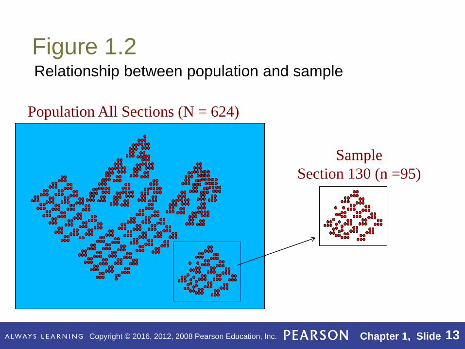
Figure 1.2Relationship between population and sample
Population All Sections (N = 624)
Copyright © 2016, 2012, 2008 Pearson Education, Inc. Chapter 1, Slide 13
Figure 1.2Relationship between population and sample
Sample
Section 130 (n =95)
Population All Sections (N = 624)

Copyright © 2016, 2012, 2008 Pearson Education, Inc. Chapter 1, Slide 14
Relationship between population and sample
STAT 2510 Example:
Sample Size %Female
n1 = 27, 70.4%
n2 = 48, 58.3%
n3 = 26, 42.3%
n4 = 95, 75.8%
n5 = 27, 70.4%
n6 = 132, 57.6%
n7 = 27, 59.3%
n8 = 93, 68.8%
n9 = 95, 66.3%
n10 = 27, 63.0%
n11 = 27, 74.1%
Population
Size: N=624
%Female: 64.9%
Statistics
Parameters

Copyright © 2016, 2012, 2008 Pearson Education, Inc. Chapter 1, Slide 15
On Your Own
Classifying Statistical Studies
(pages 4-6)
Observational Studies versus Designed Experiments

Copyright © 2016, 2012, 2008 Pearson Education, Inc. Chapter 1, Slide 16
Chapter 2Organizing Data
Copyright © 2016, 2012, 2008 Pearson Education, Inc. Chapter 2, Slide 16

Copyright © 2016, 2012, 2008 Pearson Education, Inc. Chapter 1, Slide 17
Chapter 2
Organizing Data

Copyright © 2016, 2012, 2008 Pearson Education, Inc. Chapter 1, Slide 18
Section 2.1
Variables and Data

Copyright © 2016, 2012, 2008 Pearson Education, Inc. Chapter 1, Slide 19
Definition 2.1
Variables
Variable: A characteristic that varies from one person or
thing to another.
Qualitative variable: A nonumerically valued variable.
Quantitative variable: A numerically valued variable.
Discrete variable: A quantitative variable whose possible
values can be listed. In particular, a quantitative variable
with only a finite number of possible values is a discrete
variable.
Continuous variable: A quantitative variable whose
possible values form some interval of numbers.

Copyright © 2016, 2012, 2008 Pearson Education, Inc. Chapter 1, Slide 20
Figure 2.1
Types of variables

Copyright © 2016, 2012, 2008 Pearson Education, Inc. Chapter 1, Slide 21
Definition 2.2
Data
Data: Values of a variable.
Qualitative data: Values of a qualitative variable.
Quantitative data: Values of a quantitative variable.
Discrete data: Values of a discrete variable.
Continuous data: Values of a continuous variable.

Copyright © 2016, 2012, 2008 Pearson Education, Inc. Chapter 1, Slide 22
Section 2.2
Organizing Qualitative Data

Copyright © 2016, 2012, 2008 Pearson Education, Inc. Chapter 1, Slide 23
Definition 2.3
Frequency Distribution of Qualitative Data
A frequency distribution of qualitative data is a listing of
the distinct values and their frequencies.

Copyright © 2016, 2012, 2008 Pearson Education, Inc. Chapter 1, Slide 24
Procedure 2.1

Copyright © 2016, 2012, 2008 Pearson Education, Inc. Chapter 1, Slide 25
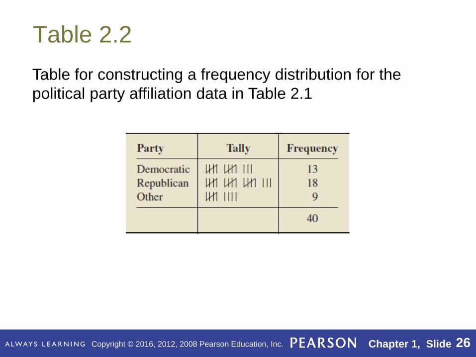
Table 2.1
Political party affiliations of the students in introductory
statistics
Copyright © 2016, 2012, 2008 Pearson Education, Inc. Chapter 1, Slide 26
Table 2.2
Table for constructing a frequency distribution for the
political party affiliation data in Table 2.1
Copyright © 2016, 2012, 2008 Pearson Education, Inc. Chapter 1, Slide 27
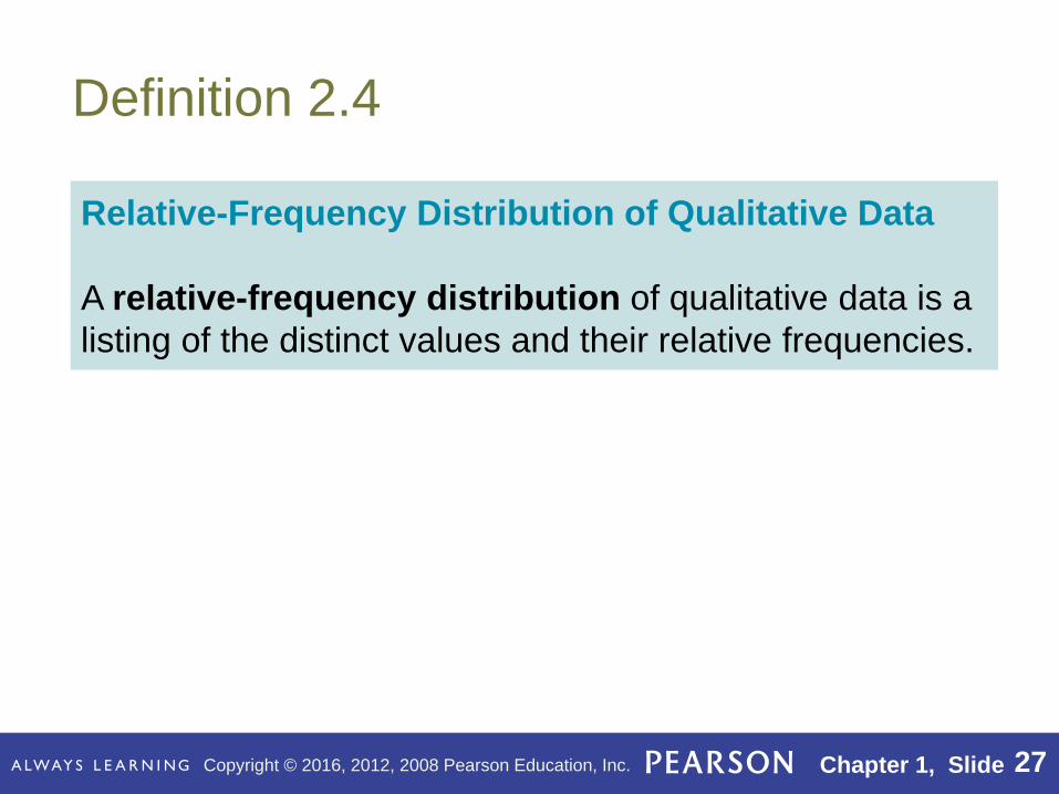
Definition 2.4
Relative-Frequency Distribution of Qualitative Data
A relative-frequency distribution of qualitative data is a
listing of the distinct values and their relative frequencies.

Copyright © 2016, 2012, 2008 Pearson Education, Inc. Chapter 1, Slide 28
Procedure 2.2

Copyright © 2016, 2012, 2008 Pearson Education, Inc. Chapter 1, Slide 29
Table 2.3
Relative-frequency distribution for the political party
affiliation data in Table 2.1

Copyright © 2016, 2012, 2008 Pearson Education, Inc. Chapter 1, Slide 30
Definition 2.5
Pie Chart
A pie chart is a disk divided into wedge-shaped pieces
proportional to the relative frequencies of the qualitative data.

Copyright © 2016, 2012, 2008 Pearson Education, Inc. Chapter 1, Slide 31
Procedure 2.3

Copyright © 2016, 2012, 2008 Pearson Education, Inc. Chapter 1, Slide 32
Figure 2.2
Pie chart of the political party affiliation data in Table 2.1

Copyright © 2016, 2012, 2008 Pearson Education, Inc. Chapter 1, Slide 33
Figure 2.2.b

Copyright © 2016, 2012, 2008 Pearson Education, Inc. Chapter 1, Slide 34
Definition 2.6
Bar Chart
A bar chart displays the distinct values of the qualitative
data on a horizontal axis and the relative frequencies (or
frequencies or percents) of those values on a vertical axis.
The relative frequency of each distinct value is represented
by a vertical bar whose height is equal to the relative
frequency of that value. The bars should be positioned so
that they do not touch each other.

Copyright © 2016, 2012, 2008 Pearson Education, Inc. Chapter 1, Slide 35
Procedure 2.4

Copyright © 2016, 2012, 2008 Pearson Education, Inc. Chapter 1, Slide 36
Figure 2.3
Bar chart of the political party affiliation data in Table 2.1

Copyright © 2016, 2012, 2008 Pearson Education, Inc. Chapter 1, Slide 37
Figure 2.3.b

Copyright © 2016, 2012, 2008 Pearson Education, Inc. Chapter 1, Slide 38
Section 2.3
Organizing Quantitative Data

Copyright © 2016, 2012, 2008 Pearson Education, Inc. Chapter 1, Slide 39
Table 2.4
Number of TV sets in each of 50 randomly selected
households.
Copyright © 2016, 2012, 2008 Pearson Education, Inc. Chapter 1, Slide 40
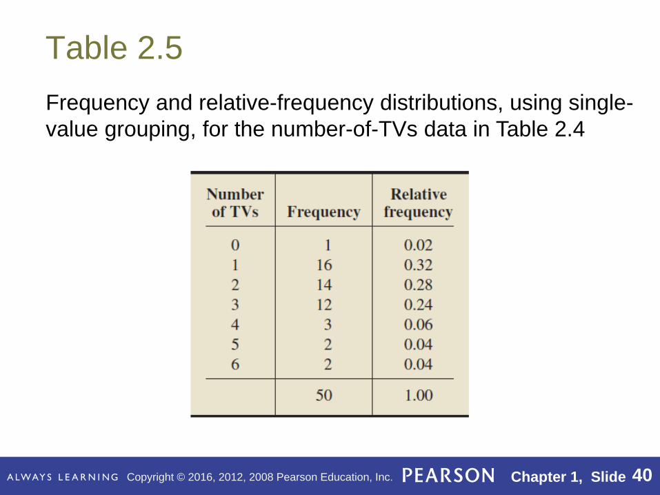
Table 2.5
Frequency and relative-frequency distributions, using single-
value grouping, for the number-of-TVs data in Table 2.4

Copyright © 2016, 2012, 2008 Pearson Education, Inc. Chapter 1, Slide 41
Table 2.6
Days to maturity for 40 short-term investments

Copyright © 2016, 2012, 2008 Pearson Education, Inc. Chapter 1, Slide 42
Table 2.6 Days to maturity for 40 short-term investments
Organizing first by ordering.
36 38 39 47 50 51 51 53
55 55 56 57 60 62 63 64
64 65 66 67 68 69 70 70
70 71 75 78 79 80 81 83
85 86 87 89 95 98 99 99

Copyright © 2016, 2012, 2008 Pearson Education, Inc. Chapter 1, Slide 43
Table 2.6 Days to maturity for 40 short-term investments
Organizing first by ordering.
36 38 39 47 50 51 51 53
55 55 56 57 60 62 63 64
64 65 66 67 68 69 70 70
70 71 75 78 79 80 81 83
85 86 87 89 95 98 99 99
Order Statistics are the ordered values of the data. The first order statistic is the
minimum, 36, the last order statistic is the maximum, 99.

Copyright © 2016, 2012, 2008 Pearson Education, Inc. Chapter 1, Slide 44
Table 2.6 Days to maturity for 40 short-term investments
Organizing first by ordering.
36 38 39 47 50 51 51 53
55 55 56 57 60 62 63 64
64 65 66 67 68 69 70 70
70 71 75 78 79 80 81 83
85 86 87 89 95 98 99 99
Order Statistics are the ordered values of the data. The first order statistic is the
minimum, 36, the last order statistic is the maximum, 99.
Is this enough summary?

Copyright © 2016, 2012, 2008 Pearson Education, Inc. Chapter 1, Slide 45
Table 2.6 Days to maturity for 40 short-term investments
Organizing first by ordering.
36 38 39 47 50 51 51 53
55 55 56 57 60 62 63 64
64 65 66 67 68 69 70 70
70 71 75 78 79 80 81 83
85 86 87 89 95 98 99 99
Order Statistics are the ordered values of the data. The first order statistic is the
minimum, 36, the last order statistic is the maximum, 99.
Is this enough summary? Since we are looking at whole numbers, maybe we
could group these data into groups of 10’s (30s, 40s, 50s, etc).

Copyright © 2016, 2012, 2008 Pearson Education, Inc. Chapter 1, Slide 46
Table 2.7
Frequency and relative-frequency distributions, using limit
grouping, for the days-to-maturity data in Table 2.6

Copyright © 2016, 2012, 2008 Pearson Education, Inc. Chapter 1, Slide 47
Definition 2.7
Terms Used in Limit Grouping
Lower class limit: The smallest value that could go in a class.
Upper class limit: The largest value that could go in a class.
Class width: The difference between the lower limit of a class
and the lower limit of the next-higher class.
Class mark: The average of the two class limits of a class.

Copyright © 2016, 2012, 2008 Pearson Education, Inc. Chapter 1, Slide 48
Frequency and relative-frequency distributions, using limit
grouping, for the days-to-maturity data in Table 2.6
Lower Class Limit
Upper Class Limit
Classes
Class width = 10 = 40 - 30 = 50 – 40 = 60 – 50 = 70 – 60 = 80 -70 = 90 - 80
Class Marks
34.5
44.5
54.5
64.5
74.5
84.5
94.5

Copyright © 2016, 2012, 2008 Pearson Education, Inc. Chapter 1, Slide 49
Cut Point Grouping (continuous data
with decimals)
129.2 185.3 218.1 182.5 142.8
155.2 170 151.3 187.5 145.6
167.3 161 178.7 165 172.5
191.1 150.7 187 173.7 178.2
161.7 170.1 165.8 214.6 136.7
278.8 175.6 188.7 132.1 158.5
146.4 209.1 175.4 182 173.6
149.9 158.6
Table 2.8 (Example 2.14): Weights of 18- to 24-
year old Males (in lbs)

Copyright © 2016, 2012, 2008 Pearson Education, Inc. Chapter 1, Slide 50
Definition 2.8
Terms Used in Cutpoint Grouping
Lower class cutpoint: The smallest value that could go in a
class.
Upper class cutpoint: The largest value that could go in the
next-higher class (equivalent to the lower cutpoint of the next-
higher class).
Class width: The difference between the cutpoints of a class.
Class midpoint: The average of the two cutpoints of a class.
Copyright © 2016, 2012, 2008 Pearson Education, Inc. Chapter 1, Slide 51
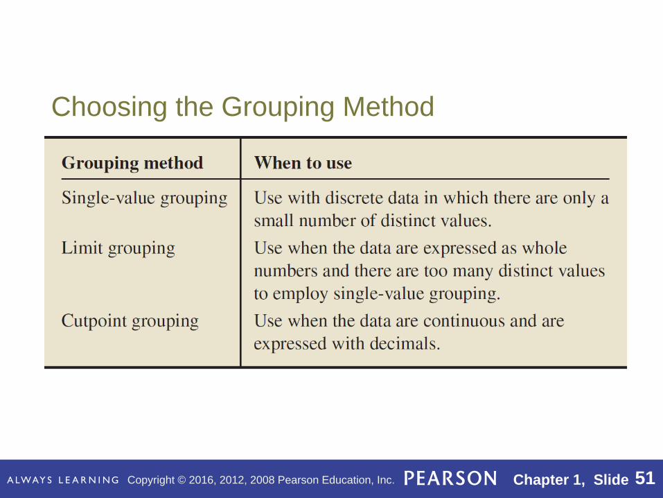
Choosing the Grouping Method

Copyright © 2016, 2012, 2008 Pearson Education, Inc. Chapter 1, Slide 52
Definition 2.9
Histogram
A histogram displays the classes of the quantitative data on a
horizontal axis and the frequencies (relative frequencies, percents) of
those classes on a vertical axis. The frequency (relative frequency,
percent) of each class is represented by a vertical bar whose height
is equal to the frequency (relative frequency, percent) of that class.
The bars should be positioned so that they touch each other.
• For single-value grouping, we use the distinct values of the
observations to label the bars, with each such value centered under
its bar.
• For limit grouping or cutpoint grouping, we use the lower class
limits (or, equivalently, lower class cutpoints) to label the bars.
Note: Some statisticians and technologies use class marks or class
midpoints centered under the bars.

Copyright © 2016, 2012, 2008 Pearson Education, Inc. Chapter 1, Slide 53
Procedure 2.5

Copyright © 2016, 2012, 2008 Pearson Education, Inc. Chapter 1, Slide 54
Figure 2.4Single-value grouping. Number of TVs per household:
(a) frequency histogram; (b) relative-frequency histogram
Copyright © 2016, 2012, 2008 Pearson Education, Inc. Chapter 1, Slide 55
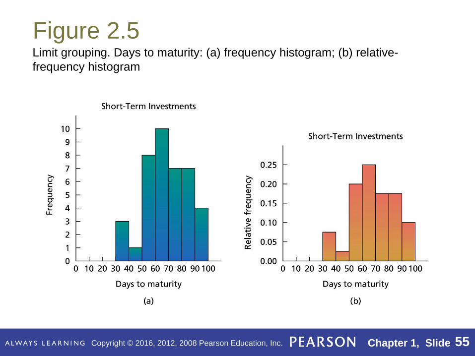
Limit grouping. Days to maturity: (a) frequency histogram; (b) relative-
frequency histogram
Figure 2.5

Copyright © 2016, 2012, 2008 Pearson Education, Inc. Chapter 1, Slide 56
Cutpoint grouping. Weight of 18- to 24-year old males: (a) frequency
histogram; (b) relative-frequency histogram
Figure 2.6

Copyright © 2016, 2012, 2008 Pearson Education, Inc. Chapter 1, Slide 57
Definition 2.10
Dotplot
A dotplot is a graph in which each observation is plotted as
a dot at an appropriate place above a horizontal axis.
Observations having equal values are stacked vertically.

Copyright © 2016, 2012, 2008 Pearson Education, Inc. Chapter 1, Slide 58
Procedure 2.6

Copyright © 2016, 2012, 2008 Pearson Education, Inc. Chapter 1, Slide 59
Table 2.11 & Figure 2.7
Prices, in dollars, of 16 DVD players

Copyright © 2016, 2012, 2008 Pearson Education, Inc. Chapter 1, Slide 60
Definition 2.11
Stem-and-Leaf Diagrams
In a stem-and-leaf diagram (or stemplot), each observation
Is separated into two parts, namely, a stem—consisting of
all but the rightmost digit– and a leaf, the rightmost digit.

Copyright © 2016, 2012, 2008 Pearson Education, Inc. Chapter 2, Slide 61
Procedure 2.7

Copyright © 2016, 2012, 2008 Pearson Education, Inc. Chapter 2, Slide 62
Table 2.13 & Figure 2.9
Cholesterol levels
for 20 high-level patients
Stem-and-leaf diagram for cholesterol levels:
(a) one line per stem; (b) two lines per stem

Copyright © 2016, 2012, 2008 Pearson Education, Inc. Chapter 2, Slide 63
Table 2.12 & Figure 2.8Days to maturity for
40 short-term investments
Constructing a stem-and-leaf diagram
for the days-to-maturity data

Copyright © 2016, 2012, 2008 Pearson Education, Inc. Chapter 2, Slide 64
Section 2.4
Distribution Shapes
Copyright © 2016, 2012, 2008 Pearson Education, Inc. Chapter 2, Slide 65
Definition 2.12
Distribution of a Data Set
The distribution of a data set is a table, graph, or
formula that provides the values of the observations and
how often they occur.

Copyright © 2016, 2012, 2008 Pearson Education, Inc. Chapter 2, Slide 66
Figure 2.10Relative-frequency histogram and approximating smooth curve
for the distribution of heights
Copyright © 2016, 2012, 2008 Pearson Education, Inc. Chapter 2, Slide 67
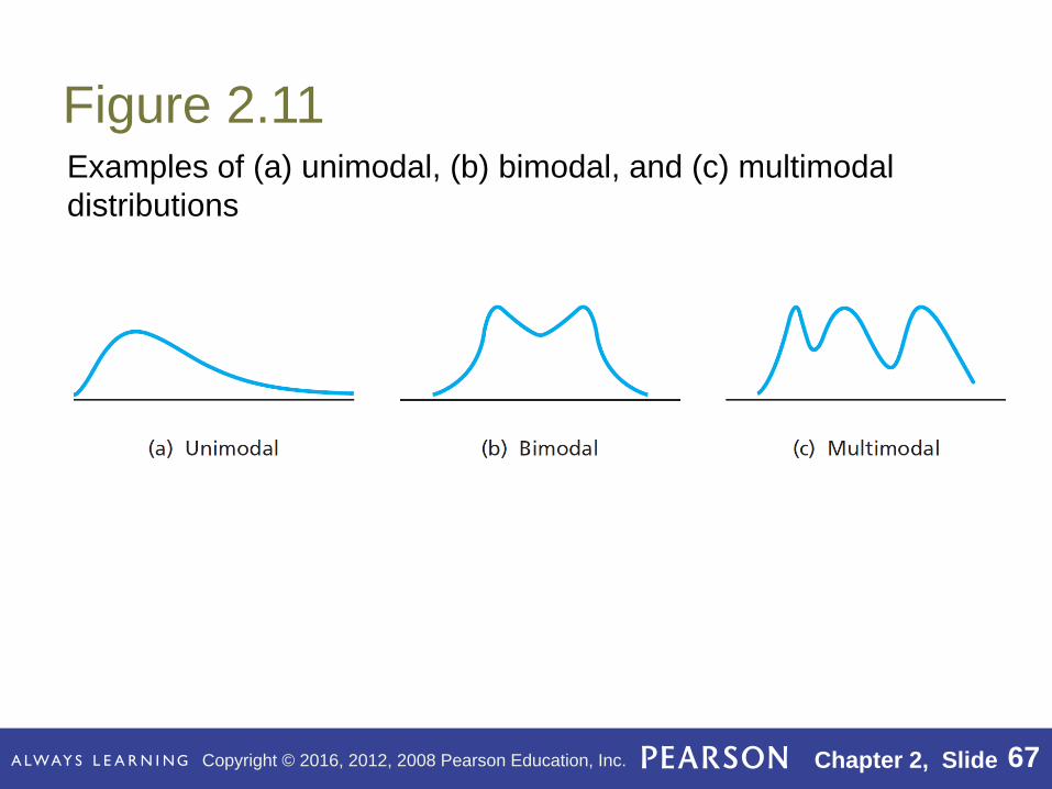
Figure 2.11Examples of (a) unimodal, (b) bimodal, and (c) multimodal
distributions

Copyright © 2016, 2012, 2008 Pearson Education, Inc. Chapter 2, Slide 68
Figure 2.12Examples of symmetric distributions: (a) bell shaped, (b) triangular,
and (c) uniform

Copyright © 2016, 2012, 2008 Pearson Education, Inc. Chapter 2, Slide 69
Figure 2.13Generic skewed distributions: (a) right skewed (b) left skewed

Copyright © 2016, 2012, 2008 Pearson Education, Inc. Chapter 2, Slide 70
Figure 2.14Reverse-J-shaped distribution

Copyright © 2016, 2012, 2008 Pearson Education, Inc. Chapter 2, Slide 71
Figure 2.15Relative-frequency histogram for household size

Copyright © 2016, 2012, 2008 Pearson Education, Inc. Chapter 2, Slide 72
Definition 2.13
Population and Sample Data
Population data: The values of a variable for the entire
population.
Sample data: The values of a variable for a sample of the
population.

Copyright © 2016, 2012, 2008 Pearson Education, Inc. Chapter 2, Slide 73
Definition 2.14
Population and Sample Distributions; Distribution of a Variable
The distribution of population data is called the population
distribution, or the distribution of the variable.
The distribution of sample data is called a sample distribution.

Copyright © 2016, 2012, 2008 Pearson Education, Inc. Chapter 2, Slide 74
Figure 2.16
Population distribution and
six sample distributions for
household size

Copyright © 2016, 2012, 2008 Pearson Education, Inc. Chapter 2, Slide 75
Key Fact 2.1
Population and Sample Distributions
For a simple random sample, the sample distribution
approximates the population distribution (i.e., the
distribution of the variable under consideration). The
larger the sample size, the better the approximation
tends to be.