The Mundell-Fleming Model Revisited

- Surajit Das∗

1. Introduction:

Incorporating the possibility of capital flows in an open economy set-up, an extension

of the closed economy IS-LM analysis (Hicks 1937) was introduced in the literature

in early 1960s by Marcus Fleming (1962) and Robert Mundell (1963). The Mundell-

Fleming (M-F now onwards) model is one of the most influential macroeconomic

models in the context of an open economy with capital flows whose presence is there

right from school text books to the highest level policy making circles. This model is

so celebrated because of its strengths lying in the following facts. Firstly, it does not

require the assumption of full employment or, in other words, it is perfectly

compatible with the Keynesian assumption of down-ward rigidity of money wages.

Secondly, it is one of the pioneering models recognising capital flows separately in

the balance of payment of any country. Thirdly, it is a simple comparative static

equilibrium framework which is easily comprehensible. And most importantly, it

deals with the basic macroeconomic aggregates of commodity market, money market

and the balance of payment including capital flows in order to determine the

aggregate level of activity and employment (given technology/ labour productivity).

The next section briefly reviews the selected literature. Section 3 deals with the

available empirical evidences. We propose our alternative model in section 4 which is

followed by a concluding section (5).

2. Selected Literature:

The essential idea behind the M-F doctrine was to link the money and the monetary

policy with the real economic activities in the context of an open economy with

capital mobility. The primary focus on the money supply (and not even on the interest

rate as an integral part of the monetary policy) made the foreign exchange market

secondary in M-F model for which the monetary stances change time to time in

reality. As Mundell himself said, later in 2001 while discussing the history of the M-F

model (Mundell 2001), that this doctrine has been developed and evolved mainly

Views are personal. Surajit Das <dasurajit@gmail.com> is at the National Institute of Public Finance & Policy (NIPFP), New Delhi. The author is deeply indebted to Prof. Prabhat Patnaik and Prof. Anjan Mukherji for their comments and inputs.

1

within IMF and also that Mundell himself was greatly influenced by Meade’s work

(1951). However, the monetary authority tries to influence the domestic interest rate

as well as the exchange rate more directly rather than controlling the aggregate money

supply in the economy per se.

The M-F model has two separate analyses - one is under fixed and another is under

flexible exchange rate assumptions. The assumption of fixed or pegged exchange rate

entails that there is little scope for monetary policy but, that the expansionary fiscal

policy may work in enhancing growth of level of activities and employment. On the

other hand, under the assumption of flexible exchange rate, if there is perfect capital

mobility, a monetary expansion leads to an increase in aggregate demand while a

fiscal or export expansion has no effect at all on the level of output and employment

even under a demand constrained situation. Expansionary fiscal policies would not be

effective because the entire additional demand would necessarily be leaked by an

equivalent import surplus1.

The crux of the argument put forward by M-F model (or popularly known as the IS-

LM-BP model) in the context of floating exchange rate and ‘perfect’ capital mobility

is as follows. In the context of an open economy, the commodity market equilibrium

equation or the IS curve is a negatively sloped schedule in the rate of interest-income

(r-Y) plane. The aggregate supply of money (Ms) is assumed to be determined

exogenously. Now if the total demand for money be the sum of transaction demand

for money (L1) and the speculative demand for money (L2), then the equation for

money market equilibrium or equation for LM curve be MS = L1(Y) + L2(r) and it is a

positively sloped curve in the r-Y plane. The BP schedule shows those combinations

of real income and real interest rates that gives equilibrium in the balance of payments

for a given exchange rate. The BP schedule is again a positively sloped schedule in r-

Y plane. Mundell-Fleming assumption under ‘perfect’ capital mobility is that if the

domestic rate of interest is higher than the world rate of interest then unlimited capital

inflow will take place and vice-versa. And ultimately domestic interest rates of the

concerned country cannot be different (exchange rate expectations and country risks

1“But this (increased government spending financed by borrowing) would increase the demand for money, raise interest rates, attract a capital inflow, and appreciate the exchange rate, which in turn would have a depressing effect on income. In fact, therefore the negative effect on income of exchange rate appreciation has to offset exactly the positive multiplier effect on income of the original increase in government spending. Income cannot change unless the money supply or interest rates change, …the change in government spending is equal to the import surplus.” – R. Mundell (1963)

2

are ignored for the time being for simplicity) from what prevails internationally. The

model in its simplest terms can be described as:

r = r* … … … (A) Ms = L(Y, r) … … … (B)

and Y = C(Y – t.Y) + I(r, Y) + G + NX(Y, e) … … …

(C)

where r is the domestic rate of interest, r* is the prevailing world rate of interest, e is

the exchange rate, NX is the net exports, t is the given tax rate (for simplicity without

loss of generality) and the other symbols have their usual meanings. r = r* because in

equilibrium it must necessarily hold and we are concerned only with equilibria. These

three equations determine the values of three unknowns viz. r, Y and e (if G is given).

In case of fixed exchange rate e is given and therefore it is money supply that

becomes an unknown or endogenously determined within the system.

There have been some extensions of Mundell-Fleming model. Michael Mussa (1976)

and Rudiger Dornbusch (1976) came out with two different papers, which were

extensions of M-F Model incorporating expectations. As has been summarised by

Michael Parkin (1976), Mussa’s paper talked about four basic propositions as follows.

First, an exchange rate is a relative price of two national monies and is determined by

the conditions for stock equilibrium in the markets for national monies and not in flow

markets for goods. Secondly, one of the factors which influence the demand for

money and, therefore, the exchange rate, is the expected future exchange rate. That

expectation is formed rationally and depends, therefore, on expected future monetary

policy. Thirdly, the exchange rate is not purely a monetary phenomenon. Real factors

which affect the demand for money also affect the exchange rate. Fourthly, the

problem of policy conflict which exists under fixed rates is modified rather than

eliminated by floating rates. Parkin (1976) commented that the modern post-

Keynesian view of the role of stock equilibrium in the money market reverses the two

links in the Fisher causation story. The proximate determinants of the price level are

now seen as the price expectations and assessments of excess demands by price

setting firms (and households) in individual markets for goods and services (and

factors of production). Given a price level thus determined, stock equilibrium in the

money market arises from interest rate and real output adjustments. In other words, it

is interest rates and real aggregate demand which are proximately determined by the

3

equality of the supply of and demand for money. Now if the exchange rates are, by

definition, relative prices of national money, then it does not follow the central

proposition of Mussa that the proximate determinants of exchange rates are the

demand for and the supplies of various national monies.

On the other hand, Dornbusch’s model is based on rational expectation and perfect

foresight – more popular as the overshooting model. Later in 2002, Kenneth Rogoff

(2002) made another extension to it. Two relationships lie at the heart of the

overshooting result. The first is the "uncovered interest parity" condition. It says that

the home interest rate on bonds, i, must equal the foreign interest rate i*, plus the

expected rate of depreciation of the exchange rate, et (i.e. et+l - et), where e is the

logarithm of the exchange rate (home currency price of foreign currency). The second

core equation of the Dorbusch model is the money demand equation: M t - Pt = -η.it+l +

φ.Yt, where M is the money supply, P is the domestic price level, and Y is domestic

output, all in logarithms; η & φ are positive parameters. Higher interest rates raise the

opportunity cost of holding money, and thereby lower the demand for money.

Conversely, an increase in output raises the transactions demand for money. Finally,

the demand for money is proportional to the price level for given Y and i. Now if for a

monetary shock, the money supply M rises relative to domestic price level P, the

interest rate i must fall for any given level of Y. If i falls relative to i*, then foreign

currency outflow takes place and the long-run impact of the money supply shock must

be a proportionate depreciation in the exchange rate. The initial depreciation of the

exchange rate must, on impact, be larger than the long-run depreciation. This initial

excess depreciation leaves room for the ensuing appreciation needed to

simultaneously clear the bond and money markets. The exchange rate must

overshoot2. But Y is assumed to be given because of underlying full employment

assumption. However, the original formulation of M-F model does not require this

assumption at all.

Patnaik & Rawal (2005) argued “It is of course true that in a world with global

mobility of finance the rates of interest (a proxy for the spectrum of returns) must be

the same in all countries (net of risk-premia); but when the rates of interest are equal

in all countries, it is not the case that capital would flow into each country exactly to

match its current account deficit. It would have an autonomy in its global pattern of

2 See, Obsfield, M & Kenneth Rogoff (1996) for the elaboration about the mechanism.

4

flows (which can of course be sought to be explained in terms of ‘expected returns’

but such an explanation would border on a tautology), the macroeconomic

consequences of which were not investigated by Mundell and Fleming whose theory

in effect precludes autonomous financial flows.”

In today’s world nobody can deny the fact that finance capital is highly mobile across

countries and it is being more and more dynamic day by day with the strengthening of

share markets, development of information technology and domestic policies of fuller

capital account convertibility, various tax concessions given to foreign investors etc.

But, particularly in the context of developing countries, the assumption of perfectly

elastic capital inflow is unrealistic. Rather, it would be more realistic to assume that a

given amount of capital (say k) becomes available to the country on the capital

account during the single period under discussion. The destination and direction of

international finance capital flows depend upon its profit opportunity net of perceived

or expected risks. Now, this profit opportunity has very little (almost nothing) to do

with the domestic interest rate of a particular economy in today’s context. It is

primarily the possibilities of capital gains based on various kinds of expectations

(investors’ confidence building spirals) and openness of the economy in terms of free

in/out flows of finance capital, which attracts the foreign institutional investments

(FIIs), which constitute a significantly large proportion of total net foreign capital

flows. Apart from FIIs, other kinds of foreign investments or disinvestments are also

dependent on profit opportunities, which are not really directly related to the rate of

interest differential (vis-à-vis any given international interest rate like FED rate or

LIBOR etc.) alone. In other words, the rate of interest is not at all a good proxy for the

spectrum of returns expected by the international finance capital.

It is true that if the domestic interest rate is too high and the cost of credit is

substantially lower elsewhere, then the domestic entrepreneurs may choose to borrow

from abroad. It is also true that if the domestic interest is too low as compared to the

internationally prevailing rate (FED rate or LIBOR) then there is a perceived risk of

capital flight. However, the point is that the net foreign capital inflow in a particular

economy and in a particular period of time should more realistically be assumed to be

exogenously given rather than assuming it to be solely dependent on the domestic

interest rate or interest rate differential or interest rate differential net of exchange rate

fluctuation etc. Interest differential may be one of the factors explaining a part of the

5

aggregate capital flow given other things equal but it is certainly not the dominant

explanatory variable of the international financial flows in today’s World. In the next

section we would elaborate this point with the help of available empirical evidences.

In such a case, in addition to the three equations there has to be a fourth one for the

balance of payment equilibrium:

NX(Y, e) = - k.e … … … … … … … … … (D)3

Now, since ‘k’ is given, the system is now over determined and the only way that

equilibrium can exist if the money supply happens to be endogenous. Therefore, even

in a world with flexible exchange rates, equilibrium in the foreign market can exist

only if money supply ceases to be exogenous. Following post-Keynesian concept of

endogenous money supply, the endogeneity does not quite depend upon the degree of

exchange rate flexibility4 as is claimed by the M-F theorization.

3. Empirical Evidences:

The M-F doctrine makes the assumption that the interest rate differential net of risk of

(expected) exchange rate fluctuation of a particular country solely causes net (in/out)

flows of foreign capital. In Indian case, for example, we have witnessed that the net

foreign capital inflows have dramatically increased particularly since 2003-04

onwards, which have resulted in a phenomenal increase in the foreign exchange

reserve of the order 320 billion US$ (almost 30% of India’s GDP) by 2007-08 from

less than 60 billion US$ during 1999-2000. But, interest rate has not increased at all

during this period. Rather, the real interest differential of India with USA has come

down quite steadily but the annual net foreign capital flow was surging up from

virtually zero in 1999-2000 to over 43 billion US$ during 2007-08. As a result of this

huge net inflow, way above the current account deficit, the foreign exchange reserves

have piled up and the exchange rate has appreciated to less than Rs.40 per US$

despite various government interventions in foreign exchange market through

sterilization, market stabilization schemes and other mechanisms. However, during

crisis of 2008-09, the exchange rate depreciated to more than Rs.50 per US$ due to

capital flight and then again there was capital inflow and exchange rate appreciation

in the recovery phase.

3 Borrowed from Patnaik, Prabhat (2001).4 See Das (2010) for a literature survey of Post-Keynesian Endogenous Money Supply.

6

Clearly, the interest differential cannot really explain the sudden surge in inflow of

foreign investment in recent past in India. This capital flow has taken place mainly in

the form of portfolio investment although foreign direct investment (may be in the

form of mergers and acquisitions or otherwise) has also increased since 2000-01.

During 2003 to 2007, the net portfolio investment (NPI) has been almost double of

the net foreign direct investment (FDI) in India. On the other hand, we find an

extremely closed relation between the BSE-SENSEX and aggregate net foreign

investment. During 2008, we have witnessed capital flight before during and after the

financial crisis in the West followed by a recovery in the recent past. The BSE-

SENSEX also moved accordingly.

The direction of flows of ever increasing international pool of finance capital can not

be seen in isolation only from one country’s point of view. How this pool gets

distributed among countries and in which proportion they fly away from various

economies needs to be discussed. It is also important to distinguish between the flow

of FDI and that of NPI. If we look at the worldwide flow of FDI during 2003-2007,

that is the period when India witnessed maximum net foreign capital inflow, we see

that the top 20 countries have received, on an average, more than 70% of entire FDI

available for all 170 countries (for which data is available). China alone has received

34% of net FDI of what was available for these top 20 countries. India has been in 8th

position with 3.33% of net FDI of top 20 countries. As far as the top 20 countries with

net outflow of FDI during 2003 to 2007 are concerned, they account for almost 100%

of entire net outflow. The US tops with 16.7%, followed by Euro countries and Japan

(see Table 1). China is getting 24% of World’s FDI and the developed World is facing

net outflow is the recent development in shift of manufacturing production base which

everybody is talking about.

The data source is International Financial Statistics (IFS) 2009 provided by the

International Monetary Fund (IMF). For Indian data on trade deficit, exchange rate

(Rs./US$), international price of oil and petroleum product of Indian basket, and

domestic GDP at current market price, the source is Handbook of Statistics on Indian

Economy, 2009 provided by the Reserve Bank of India (RBI), Government of India.

7

Table 1: Top 20 Countries in Terms of FDI In/Outflow During 2003 to 2007

Net FDI Inflow(In US Million $)

% of Top 20

Net FDI Outflow(In US Million $)

% of Top 20

CountryAnnual Average Countries Country

Annual Average Countries

China,P.R.: Mainland 69307 34.06 United States -54936 -16.68Mexico 16612 8.17 Spain -39422 -11.97Poland 10340 5.08 Japan -39232 -11.91Turkey 10276 5.05 Germany -38396 -11.66Singapore 9864 4.85 France -34982 -10.62Brazil 9847 4.84 Switzerland -23859 -7.24Romania 7076 3.48 Netherlands -18397 -5.59India 6780 3.33 Italy -14304 -4.34Thailand 6652 3.27 Luxembourg -14266 -4.33Belgium 6610 3.25 Ireland -13724 -4.17Australia 6504 3.20 Sweden -10987 -3.34Czech Republic 5873 2.89 Norway -9017 -2.74Chile 5644 2.77 Kuwait -4827 -1.47Egypt 5480 2.69 Iceland -3250 -0.99Ukraine 5122 2.52 Denmark -3158 -0.96Bulgaria 4997 2.46 Korea -2305 -0.70Kazakhstan 4675 2.30 Austria -1711 -0.52Colombia 4588 2.25 Saudi Arabia -1573 -0.48Canada 3799 1.87 China,P.R.:Hong Kong -762 -0.23Finland 3411 1.68 Venezuela, Rep. Bol. -247 -0.08

Source: Calculated from International Financial Statistics, IMF, 2009.

Similarly, if we look at the worldwide flows of portfolio capital, we see that, on an

average, the top 20 countries receive 98% of the entire NPI availability for 150

countries (for which data is available) during 2003 to 2007. Again, the top 20

countries facing an outflow of NPI account for 96% of all outflows. USA alone

attracts 60% of NPI, and India was in 10th position with 1.25% of NPI among top 20

countries during 2003-2007. Countries which were experiencing portfolio capital

outflow are France, Saudi Arabia, Switzerland, Norway, Cinese province of Hong

Kong, Canada, Belgium etc. Apart from US, countries which have experienced

significant net portfolio capital inflow are Spain, Luxemburg, UK, Germany, Italy,

Australia, Japan, Greece etc. Net FDI inflow in all countries receiving positive FDI is

just one fourth of NPI on an average during 2003-07.

8

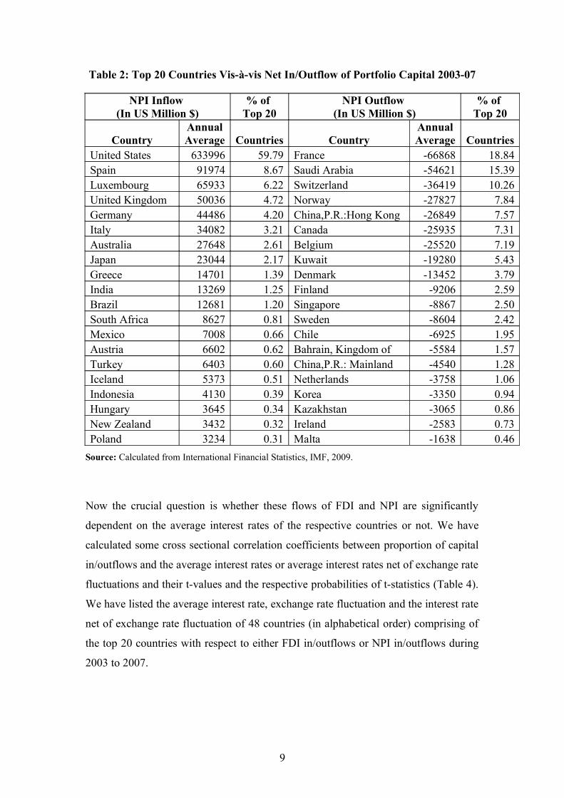
Table 2: Top 20 Countries Vis-à-vis Net In/Outflow of Portfolio Capital 2003-07

NPI Inflow (In US Million $)

% of Top 20

NPI Outflow (In US Million $)

% of Top 20

CountryAnnual Average Countries Country

Annual Average Countries

United States 633996 59.79 France -66868 18.84Spain 91974 8.67 Saudi Arabia -54621 15.39Luxembourg 65933 6.22 Switzerland -36419 10.26United Kingdom 50036 4.72 Norway -27827 7.84Germany 44486 4.20 China,P.R.:Hong Kong -26849 7.57Italy 34082 3.21 Canada -25935 7.31Australia 27648 2.61 Belgium -25520 7.19Japan 23044 2.17 Kuwait -19280 5.43Greece 14701 1.39 Denmark -13452 3.79India 13269 1.25 Finland -9206 2.59Brazil 12681 1.20 Singapore -8867 2.50South Africa 8627 0.81 Sweden -8604 2.42Mexico 7008 0.66 Chile -6925 1.95Austria 6602 0.62 Bahrain, Kingdom of -5584 1.57Turkey 6403 0.60 China,P.R.: Mainland -4540 1.28Iceland 5373 0.51 Netherlands -3758 1.06Indonesia 4130 0.39 Korea -3350 0.94Hungary 3645 0.34 Kazakhstan -3065 0.86New Zealand 3432 0.32 Ireland -2583 0.73Poland 3234 0.31 Malta -1638 0.46

Source: Calculated from International Financial Statistics, IMF, 2009.

Now the crucial question is whether these flows of FDI and NPI are significantly

dependent on the average interest rates of the respective countries or not. We have

calculated some cross sectional correlation coefficients between proportion of capital

in/outflows and the average interest rates or average interest rates net of exchange rate

fluctuations and their t-values and the respective probabilities of t-statistics (Table 4).

We have listed the average interest rate, exchange rate fluctuation and the interest rate

net of exchange rate fluctuation of 48 countries (in alphabetical order) comprising of

the top 20 countries with respect to either FDI in/outflows or NPI in/outflows during

2003 to 2007.

9

Table 3: Interest Rate & Exchange Rate Fluctuation of 48 Countries 2003-07

Annual Average 2003 to 2007 Annual Average 2003 to 2007

CountryInterest Rate %

Exchange Rate (%) Fluctuation

Net Interest Rate % Country

Interest Rate %

Exchange Rate (%) Fluctuation

Net Interest Rate %

Australia 9.15 -7.98 1.17 Japan 1.76 -1.12 0.65

Austria 7.64 -7.00 0.64 Kazakhstan 8.40 -4.34 4.06

Bahrain, Kingdom of 8.14 0.00 8.14 Korea 6.05 -5.73 0.32

Belgium 7.57 -7.00 0.56 Kuwait 7.14 -1.36 5.78

Brazil 54.38 -7.46 46.93 Luxembourg 3.94 -7.00 -3.07

Bulgaria 8.99 -7.02 1.97 Malta 5.71 -6.18 -0.46

Canada 5.00 -7.36 -2.36 Mexico 7.85 2.63 10.48

Chile 6.93 -5.28 1.65 Netherlands 7.95 -7.00 0.95

China,P.R.: Mainland 6.01 -1.66 4.35 New Zealand 11.36 -8.36 3.00

China,P.R.:Hong Kong 6.45 0.00 6.45 Norway 4.87 -5.92 -1.05

Colombia 14.62 -3.14 11.48 Poland 10.11 -7.40 2.70

Czech Republic 5.83 -9.08 -3.25 Romania 9.60 -5.77 3.83

Denmark 5.90 -6.96 -1.06 Saudi Arabia 6.00 0.00 6.00

Egypt 13.03 7.09 20.12 Singapore 5.31 -3.34 1.97

Finland 8.61 -7.00 1.61 South Africa 12.24 -6.76 5.49

France 6.60 -7.00 -0.40 Spain 8.57 -7.00 1.56

Germany 9.18 -7.00 2.18 Sweden 4.44 -6.81 -2.38

Greece 13.03 -7.00 6.03 Switzerland 3.15 -4.96 -1.81

Hungary 9.63 -6.30 3.33 Thailand 6.33 -4.23 2.09

Iceland 15.19 -6.47 8.72 Turkey 28.31 -2.80 25.51

India 11.47 -3.11 8.35 Ukraine 16.11 -1.06 15.04

Indonesia 14.99 -0.18 14.81 United Kingdom 4.58 -5.60 -1.02

Ireland 8.96 -7.00 1.96 United States 6.13 0.00 6.13

Italy 10.78 -7.00 3.78 Venezuela, Rep. Bol. 18.62 13.93 32.55Source: Calculated from International Financial Statistics, IMF, 2009.

Another interesting observation is that the 32 countries are common in the list of 40

countries of FDI (in/outflow) and in the list of 40 countries of NPI (in/outflow). It is

important to note here that countries like USA, Japan, Spain, Germany, Italy,

Luxembourg etc. are facing huge net FDI outflow during 2003-07 whereas, at the

same time they are experiencing large NPI inflow. Again, countries like China,

Belgium, Finland, Chile, Kazakhstan, Singapore etc. are experiencing NPI outflow

but receiving huge FDI inflow at the same time. Therefore, it is not necessary at all

that both the flows would take place in the same direction depending on their net

interest rate differentials.

10

Table 4: Correlation Between Capital Flows and Interest RatesDependent Variable Independent Variable Corr

Coeff.P(t)

Average net FDI outflow of a particular country as % of average net FDI outflow of 20 countries 2003-07

Average interest rate of respective countries during 2003-07

(-)0.27 0.24

Average net FDI outflow of a particular country as % of average net FDI outflow of top 20 countries during 2003-07

Average interest rate net of average exchange rate fluctuation of respective countries during 2003-07

(-)0.24 0.31

Average net FDI inflow of a particular country as % of average net FDI inflow of top 20 countries 2003-07

Average interest rate of respective countries during 2003-07

(-)0.07 0.75

Average net FDI inflow of a particular country as % of average net FDI inflow of top 20 countries during 2003-07

Average interest rate net of average exchange rate fluctuation of respective countries during 2003-07

0.00 0.99

Average net FDI in/outflow of a particular country as % of average net FDI in/outflow of top 40 countries during 2003-07

Average interest rate of respective countries during 2003-07

0.18 0.28

Average net FDI in/outflow of a particular country as % of average net FDI in/outflow of top 40 countries during 2003-07

Average interest rate net of average exchange rate fluctuation of respective countries during 2003-07

0.20 0.20

Average NPI outflow of a particular country as % of average NPI outflow of top 20 countries during 2003-07

Average interest rate of respective countries during 2003-07

(-)0.32 0.17

Average NPI outflow of a particular country as % of average NPI outflow of top 20 countries during 2003-07

Average interest rate net of average exchange rate fluctuation of respective countries during 2003-07

(-)0.06 0.79

Average NPI inflow of a particular country as % of average NPI inflow of top 20 countries during 2003-07

Average interest rate of respective countries during 2003-07

(-)0.18 0.45

Average NPI inflow of a particular country as % of average NPI inflow of top 20 countries during 2003-07

Average interest rate net of average exchange rate fluctuation of respective countries during 2003-07

(-)0.09 0.72

Average NPI in/outflow of a particular country as % of average NPI in/outflow of top 40 countries 2003-07

Average interest rate of respective countries during 2003-07

0.04 0.81

Average NPI in/outflow of a particular country as % of average NPI in/outflow of top 40 countries during 2003-07

Average interest rate net of average exchange rate fluctuation of respective countries during 2003-07

0.09 0.57

Source: Calculated from International Financial Statistics, IMF, 2009.

11

Clearly, the above empirical evidence suggests that there is insignificant correlation

between FDI or NPI flows and the interest rates or that net of exchange rate

fluctuations. However, external commercial borrowings may be related to the interest

rate differential. But, these flows of FDI and NPI dominate the capital account and

that in turn dominates the current account or the trade balance in countries with huge

capital flows. The above mentioned empirical evidences substantiate the proposition

that the direction origin and destination of international flows of finance capital are

not solely determined by the interest rate differential for sure. Other factors dominate.

In that sense it is exogenous from any single country’s point of view. The so called

‘investment friendly environment’, government guarantees like ‘full capital account

convertibility and tax concession on capital gains for the foreign investors in the share

markets, easy mobility of finance capital due to development of information

technology and internet banking etc. are anyway out of the scope of the M-F

framework. Even if, the interest parity is maintained all over the World after

adjustments for various country risks and exchange rate fluctuations in forward

market, then also the finance capital would move in search of profit. This expected

rate of profit has very little to do with the domestic interest rates.

However, these flows of finance capital affects the exchange rate significantly, which

in turn affects the trade deficit. For example, in Indian case, the exchange rate

fluctuation has very strong and significant effect on the trade deficit and in turn on the

aggregate level of activity. If the exchange rate appreciates then historically the trade

deficit increases at least in Indian case and dampens the level of activity and

employment. If we regress the logarithm of trade deficit of India with respect to

logarithm of Indian exchange rate vis-à-vis US dollar (Rs./US$), logarithm of India’s

GDP at current market price and logarithm of the international price of Indian basket

of oil and petroleum products, we get a negative significant relationship with the

exchange rate with partial elasticity of 2.4 during the period 1977-78 to 2007-08. As

expected, the trade deficit is a positive function of domestic GDP (as import demand

rises with GDP) and a positive function of international price of oil and petro-

products of the average Indian basket (as it inflates the import bill given relatively

inelastic demand for oil). The model is fairly good fit with R2 being 96.66% and DW-

Stat being exact 2 with a dummy for 1998-99 capturing the possible post South East

Asian crisis effect. The residual is fairly stationary.

12

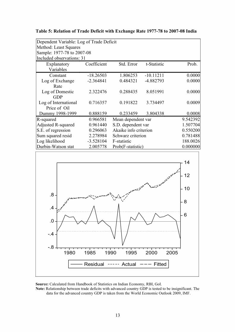
Table 5: Relation of Trade Deficit with Exchange Rate 1977-78 to 2007-08 India

Dependent Variable: Log of Trade DeficitMethod: Least SquaresSample: 1977-78 to 2007-08Included observations: 31

Explanatory Variables

Coefficient Std. Error t-Statistic Prob.

Constant -18.26503 1.806253 -10.11211 0.0000Log of Exchange

Rate-2.364841 0.484321 -4.882793 0.0000

Log of Domestic GDP

2.322476 0.288435 8.051991 0.0000

Log of International Price of Oil

0.716357 0.191822 3.734497 0.0009

Dummy 1998-1999 0.888159 0.233459 3.804338 0.0008R-squared 0.966581 Mean dependent var 9.542392Adjusted R-squared 0.961440 S.D. dependent var 1.507704S.E. of regression 0.296063 Akaike info criterion 0.550200Sum squared resid 2.278984 Schwarz criterion 0.781488Log likelihood -3.528104 F-statistic 188.0026Durbin-Watson stat 2.005778 Prob(F-statistic) 0.000000

-.8

-.4

.0

.4

.8

6

8

10

12

14

1980 1985 1990 1995 2000 2005

Residual Actual Fitted

Source: Calculated from Handbook of Statistics on Indian Economy, RBI, GoI.Note: Relationship between trade deficits with advanced country GDP is tested to be insignificant. The

data for the advanced country GDP is taken from the World Economic Outlook 2009, IMF.

13

4. The Proposed Model:

Now if the money supply happens to be endogenously determined and the net foreign

capital inflow happens to be exogenous then in a simple comparative static

framework, then some of the obvious corollaries of M-F model get reversed. The M-F

postulate is that the product and the money market equilibrium conditions would

determine the overall level of activity and employment in the economy irrespective of

the situation of the balance of payment and the capital flow would always

automatically necessarily adjust to it under flexible exchange rate. We believe that it

would be more realistic to assume that the macroeconomic equilibrium is determined

through the simultaneous equilibrium in commodity market and balance of payment

and the money market automatically always adjust to that equilibrium in the context

of an open economy with free capital flows. Capital flow is not a passive residual

variable as was postulated by the M-F doctrine but, in today’s context it is one of the

crucial exogenous variable which actively affect the level of activity and employment

in an economy. For a formal derivation, let us assume some standard relationships in

their simplest linear5 form as follows:

The national income identity or the commodity market equilibrium condition is given

by

Y = C(Y – T) + I(r, Y) + G + X(e) – M(Y, e) … … … … (1)

where Y is aggregate income, C is consumption, T is tax, I is investment, r is rate of

interest, G is government spending, X is export, e is the exchange rate and M is the

import.

Standard tax function, when the tax-GDP ratio is assumed to be given takes the form

T = t.Y … … … … (2)

where t is constant tax-GDP ratio.

The consumption as a positive function of disposable income is given by

C = θ + c.(Y – T) = θ + c.Y(1 – t) … … … … (3) [since, (2)]

where θ is an arbitrary positive (+ve) constant.

The investment function is assumed to depend positively on Y and negatively on r as

5 See Das (2008) for generalised derivation without the assumption of linearity and the stability condition.

14

I = λ + α.Y – β.r = δ + α.Y … … … … (4)

where λ, α, β and δ are arbitrary +ve constants and δ = λ – β.r* when r = r*

administered.

The export function is given as positive function of the exchange rate and hence

competitiveness

X = μ + e.x … … … … (5)

where μ and x are arbitrary constants

And the import as a positive function of Y and negative function of e is given as

M = ρ + m.Y – e.n … … … … (6)

Therefore, from (1) we get the commodity market equilibrium condition as,

Y = θ + c.Y(1 – t) + δ + α.Y + G + μ + e.x – (ρ + m.Y – e.n)

⇒ Y.[1 – c.(1 – t) – α + m] = φ + e.(x + n) … … … … (7)

where φ = θ + δ + G + μ –ρ.

The equilibrium condition for the balance of payment (BoP) in foreign exchange

market be

ρ + m.Y – e.n – (μ + e.x) = k.e = K … … … … (8)

i.e. current account deficit is equal to net foreign capital inflow in terms of domestic

currency.

The above equation (7) tells us the relationship between e & Y for commodity market

equilibrium and equation (8) gives the relationship between e & Y in BoP

equilibrium. For fixed exchange rate e = e*, we get a solution for Y from this equation

itself. Y = (k.e* +X – A)/m = Y*

For flexible exchange rate to get a unique solution for e & Y we need equilibrium in

commodity and foreign exchange market simultaneously.

From (7) we get the slope of the commodity market equilibrium condition as

de/dY = [1 – c.(1 – t) – α + m]/(x + n) … … … … (9)

From (8) we get the slope of the foreign exchange market BoP equilibrium condition

as

15

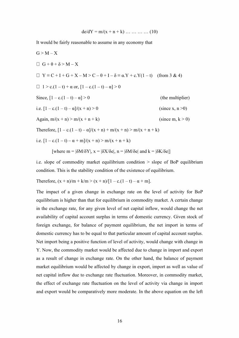
de/dY = m/(x + n + k) … … … … (10)

It would be fairly reasonable to assume in any economy that

G > M – X

⇒ G + θ + δ > M – X

⇒ Y ≡ C + I + G + X – M > C – θ + I – δ ≡ α.Y + c.Y(1 – t) (from 3 & 4)

⇒ 1 > c.(1 – t) + α or, [1 – c.(1 – t) – α] > 0

Since, [1 – c.(1 – t) – α] > 0 (the multiplier)

i.e. [1 – c.(1 – t) – α]/(x + n) > 0 (since x, n >0)

Again, m/(x + n) > m/(x + n + k) (since m, k > 0)

Therefore, [1 – c.(1 – t) – α]/(x + n) + m/(x + n) > m/(x + n + k)

i.e. [1 – c.(1 – t) – α + m]/(x + n) > m/(x + n + k)

[where m = |δM/δY|, x = |δX/δe|, n = |δM/δe| and k = |δK/δe|]

i.e. slope of commodity market equilibrium condition > slope of BoP equilibrium

condition. This is the stability condition of the existence of equilibrium.

Therefore, (x + n)/m + k/m > (x + n)/[1 – c.(1 – t) – α + m].

The impact of a given change in exchange rate on the level of activity for BoP

equilibrium is higher than that for equilibrium in commodity market. A certain change

in the exchange rate, for any given level of net capital inflow, would change the net

availability of capital account surplus in terms of domestic currency. Given stock of

foreign exchange, for balance of payment equilibrium, the net import in terms of

domestic currency has to be equal to that particular amount of capital account surplus.

Net import being a positive function of level of activity, would change with change in

Y. Now, the commodity market would be affected due to change in import and export

as a result of change in exchange rate. On the other hand, the balance of payment

market equilibrium would be affected by change in export, import as well as value of

net capital inflow due to exchange rate fluctuation. Moreover, in commodity market,

the effect of exchange rate fluctuation on the level of activity via change in import

and export would be comparatively more moderate. In the above equation on the left

16

hand side not only the positive factor (k/m) is extra but also (x + n)/m > (x + n)/ [1 –

c.(1 – t) – α + m]. Taking reciprocal in both sides we get,

m/(x + n) < m/(x + n) +[1 – c.(1 – t) – α]/(x + n)

[1 – c.(1 – t) – α]/(x + n) > 0 always. Therefore, the effect would be moderate.

From equation (7) & (8) we get a solution for e & Y in the following manner:

Equation (7) implies that Y = [φ + e.(x + n)]/[1 – c.(1 – t) – α + m]

From equation (8) we get, Y = [k.e + e.n + (μ + e.x)]/m

For simultaneous equilibrium in both the markets equating these two we get,

e(k + n + x)/m – e.(x + n)/[1 – c.(1 – t) – α + m] = φ/[1 – c.(1 – t) – α + m] – μ/m.

⇒ e* = (φ.m – μ.m – μ.ξ)/[ξ.(x + n +k) + m.k] … … … … (11)

⇒ Y* = [(φ.m – μ.m – μ.ξ).(k + n + x)]/[m.{ξ.(x +n +k) + m.k}] + μ/m … … (12)

[from (8)]

where ξ = [1 – c.(1 – t) – α]

Therefore, coordinate (Y*, e*) in e-Y plane is a particular combination of exchange

rate and income where both the commodity and the foreign exchange market would

be in equilibrium simultaneously.

Now, let us see the effect of change in government expenditure G and the net capital

inflow k on the exchange rate e and aggregate output Y in a comparative static

framework. If, for example G rises by ΔG, ceteris paribus, then Y changes by ΔY and

e changes by Δe. Now, if G increases by ΔG, then φ also increases by ΔG. Therefore,

from (12) we get,

ΔY* = ΔG.m.(k + n + x)/[m.{ξ.(x +n +k) + m.k}]

⇒ ΔY*/ ΔG = m.(k + n + x)/[m.{ξ.(x +n +k) + m.k}] [Since ξ = {1 – c.(1 – t) – α}]

⇒ ΔY*/ ΔG = (k + n + x)/[{1 – c.(1 – t) – α}.(x +n +k) + m.k] … … … (13)

And from equation (11) we get,

Δe* = ΔG.m/[ξ.(x +n +k) + m.k]

⇒ Δe*/ ΔG = m/[ξ.(x +n +k) + m.k] [Since ξ = {1 – c.(1 – t) – α}]

17

⇒ Δe*/ ΔG = m/[.[{1 – c.(1 – t) – α}.(x +n +k) + m.k] … … … … (14)

Therefore, we get, (ΔY*/ ΔG)>0 as well as (Δe*/ ΔG)>0. Hence, if G increases,

ceteris paribus, both Y and e unambiguously rises and vice-versa for any given level

of net capital inflow k.

Similarly if k rises by Δk, Y* becomes Y1* and e* becomes e1*. Therefore, from (12)

we get,

Y1* = [Δk(φ.m – μ.m – μ.ξ) + (k + n + x).(φ.m – μ.m – μ.ξ)]/[ Δk.m.(ξ +m) + m.{ξ(k

+ n + x) + m.k} + μ/m … … … (15)

Now, Y1* would be less than Y* if the percentage rise in the numerator is less than

the percentage increase in the denominator (hence the ratio comes down) and vice-

versa.

Δk(φ.m – μ.m – μ.ξ)/[(k + n + x).(φ.m – μ.m – μ.ξ)]<{Δk.m.(ξ +m)}/ {m.{ξ(k

+ n + x) + m.k}

i.e. Δk/(k + n + x) < Δk.(ξ +m)/{ξ(k + n + x) + m.k}

i.e. 1/(k + n + x) < (ξ +m)/{ξ(k + n + x) + m.k}

i.e. ξ(k + n + x) + m.k < (k + n + x).(ξ +m)

i.e. mk < (k + n + x).m

i.e. k < k + n + x

i.e. n + x > 0, but this is always true because by assumption both n and x are positive.

Therefore, if net capital inflow increases, then necessarily Y declines to keep both the

product and the foreign exchange market in equilibrium.

Similarly, from (11) we get,

e1* = (φ.m – μ.m – μ.ξ)/[ Δk.(ξ +m) + ξ.(k +n +x) +m.k] … … … … (16)

Now, e* > e1* if Δk.(ξ +m) > 0, this is always true because Δk, ξ, and m are positive.

Therefore, if net capital inflow increases, then necessarily the exchange rate

appreciates to keep both the product and the foreign exchange market in equilibrium.

Hence, the ultimate effect of an expansion of autonomous demand on level of activity

is positive and net capital inflow eventually reduces the level of employment and

output under the flexible exchange rate.

18

5. Conclusion:

Here we are significantly deviating from the M-F doctrine in the following manner.

Firstly, we are saying that the e* & Y* are determined by goods market and foreign

exchange market equilibria and the money market would always be in equilibrium at

any rate of interest or in other words the money supply would be endogenously

determined according to the demand for it6. In M-F model, as opposed to that, under

flexible exchange rate the equilibrium is determined through intersection of

commodity market equilibrium condition and money market equilibrium condition

subject to an exogenous aggregate money supply and the foreign exchange market

always adjusts to that common equilibrium point automatically. Secondly, we are

claiming here that the net foreign capital inflow is not really directly dependent on the

interest rates differentials; rather, it would be more realistic to assume that the net

capital flows into or out of a particular economy to be exogenously determined at any

particular period of time. Particularly in today’s context, when most of the foreign

capital flows take place through share markets in terms of foreign institutional

investment, it will be exaggeration to say that the profit or loss opportunity of foreign

investment would depend solely on the interest rate differential even after adjustment

of expected exchange rate fluctuations. Rather the direction and destination of

international finance capital would be driven by profit motive based on expected

capital gains (profit) net of various kinds of country risks.

Net export is a positive function of the exchange rate (NX = k.e) because if the

exchange rate increases (i.e. depreciation), exporters would get more price as export

earning and their competitiveness increases and importables become comparatively

more expensive and as a result reduces. On the other hand, if the exchange rate

appreciates then, the importers would be encouraged to import more at a relatively

cheaper rate and exporters would be discouraged as their competitiveness would fall.

The domestic production would be substituted by relatively cheaper imported inputs

given any fixed rate of import duties and as an obvious consequence de-

industrialization takes place in an open economy exposed to foreign capital flows

under flexible exchange rate regime (necessarily if the Marshall-Lerner condition

holds7). Therefore, we get a positive function of aggregate demand Y with the

exchange rate for commodity market equilibrium. If autonomous components of 6 See (among others) Kaldor N. (1958), Robinson J. (1970), Moore B. J. (1988), Pollin R. (1991).7 See Sodersten, B (1980)

19

consumption or investment or the government expenditure increase then for each

levels of exchange rate we would get larger level of aggregate demand and larger

amount of Y and as a result the commodity market equilibrium function shifts

parametrically.

In absence of any increase in autonomous demand, due to larger net capital inflow the

exchange rate would appreciate and the employment and output would fall (however,

the opposite is not true8) under a flexible exchange rate regime. If autonomous

demand, for example government expenditure, increases, cet par, then the level of

activity would increase. However, if the foreign capital inflow helps domestic demand

to boost up by increasing, for example, investment, exports or government

expenditure, then also the commodity market equilibrium condition or the IS schedule

shifts rightward increasing the level of activity. If both net capital inflow as well as

autonomous demand increases simultaneously then the net effect on the level of

activity would depend on which effect more that offsets what. Therefore, under such a

situation under flexible exchange rate and with larger net capital inflow the

expansionary fiscal policy would definitely work but, its effect would be dampened

on expansion of employment and the level of activity.

For fixed exchange rate, the overall aggregate level of activity is solely determined by

the commodity market equilibrium condition. As opposed to the essential corollary of

the M-F doctrine that the expansionary fiscal policy would be completely ineffective,

we are concluding that under the assumption of Keynesian downward wage rigidity in

the presence of persisting involuntary unemployment and money supply endogeniety,

given any tax rate, the expansionary fiscal policy unambiguously increases

employment and output when the exchange rate is flexible. Again, the increase in net

foreign capital inflow, ceteris paribus, reduces the level of employment and output.

Therefore, the demand expansion has to be large enough to more than offset this

dampening effect or the foreign capital flows have to be controlled or some

combination of these two. Therefore, the expansionary fiscal policies coupled with

some control over foreign capital flows are recommended as opposed to conservative

fiscal stance along with absolutely reckless capital flows that we are witnessing today.

8 For an explanation see Patnaik, Prabhat & Vikas Rawal (2005).

20

References:

Das, Surajit (2010) – “On Financing the Fiscal Deficit and Availability of Loanable Funds in India”, Economic & Political Weekly Vol. XLV No. 15, pp. 67-75, April 10.

Das, Surajit (2008) – “Macroeconomic Policy Under A Regime of Free Capital Flows”, PhD thesis, Jawaharlal Nehru University, New Delhi.

Dornbusch, Rudiger (1976) – "Expectations and Exchange Rate Dynamics" Journal of Political Economy, Vol. 84, pp. 1161-76.

Fleming, Marcus (1962) – “Domestic Financial Policies Under Fixed and Flexible Exchange Rates”, IMF Staff Papers, Vol.19, No.3.

Hicks, John R. (1937) – “Mr. Keynes and the Classics: A Suggested Interpretation”, Econometrica, Vol. 5 No. 2, pp. 147-159, April.

International Monetary Fund (2009) – International Financial Statistics Database.International Monetary Fund (2009) – World Economic Outlook Database.Kaldor Nicholas (1958) – “Monetary Policy, Economic Stability and Growth”, A

Memorandum Submitted to the Committee of the Working of the Monetary System (Radcliffe Committee), June 23. Reprinted in Collected Economic Papers, Volume 3. Essays on Economic Policy I, London, Duckworth, 1964.

Meade, James E. (1951) – The Balance of Payments (London; New York: OUP).Moore, Basil J. (1988) – Horizontalists and Verticalists – The Macroeconomics of

Credit Money, Cambridge University Press.Mundell, Robert A. (2001) – “On the history of the Mundell-Fleming Model”, IMF

Staff Papers, Vol. 47, Special Issue, International Monetary Fund.Mundell, Robert A. (1963) – “Capital Mobility and Stabilization Policy under Fixed

and Flexible Exchange Rates”, The Canadian Journal of Economics and Political Science, Vol. 29, No. 4, pp. 475-485, November.

Mussa, M. (1976) – “The Exchange Rate, the Balance of Payments, and Monetary and Fiscal Policy Under a Regime of Controlled Floating”, Scandinavian Journal of Economics, Vol. 78 No. 2, pp. 229-248.

Obsfield, Maurice & Kenneth Rogoff (1996) – Foundations of International Macroeconomics, The MIT Press, Massachusetts.

Parkin, Michael (1976) – “Comment on Mussa”, Scandinavian Journal of Economics, Vol. 78 No. 2, pp. 249-254.

Patnaik, Prabhat & Vikas Rawal (2005) – “Level of Activity in An Economy With Free Capital Mobility” Economic and Political Weeky, April 2; pp. 1449 – 57.

Patnaik, Prabhat (2001) – “Capital Mobility and Open-economy Macroeconomics”, in Indian Economy: Agenda for the 21st Century: Essays in Honour of P. R. Brahmananda (ed.) Raj Kumar Sen and Biswajit Chatterjee, Deep and Deep publication Private Limited, New Delhi.

Pollin Robert (1991) – “Two Theories of Money Supply Endogeneity: Some Empirical Evidence”, Journal of Post Keynesian Economics, Vol. 13 No. 3, pp. 366-95.

Reserve Bank of India (2010) – Handbook of Statistics on Indian Economy Database.Robinson Joan (1970) – “Quantity Theories Old and New: Comment”, Journal of

Money, Credit and Banking, Vol. 2 No. 4, pp. 504-12.Rogoff, Kenneth (2002) – “Dornbusch's Overshooting Model After Twenty-Five

Years”, International Monetary Fund's Second Annual Research Conference Mundell-Fleming Lecture, IMF Staff Papers, Vol. 49, pp. 1-34.

Sodersten, B (1980) – International Economics, The McMillan Press Ltd, London.

21