the modern tools of quantum mechanics - arxiv · way that quantum mechanics is taught, both at...

EPJ manuscript No.(will be inserted by the editor)

The modern tools of quantum mechanics

A tutorial on quantum states, measurements, and operations

Matteo G A Paris1,2,3

1 Dipartimento di Fisica dell’Universita degli Studi di Milano, I-20133 Milano, Italia, EU2 CNISM - Udr Milano, I-20133 Milano, Italia, EU.3 e-mail: [email protected]

Abstract. We address the basic postulates of quantum mechanics andpoint out that they are formulated for a closed isolated system. Sincewe are mostly dealing with systems that interact or have interactedwith the rest of the universe one may wonder whether a suitable modi-fication is needed, or in order. This is indeed the case and this tutorialis devoted to review the modern tools of quantum mechanics, which aresuitable to describe states, measurements, and operations of realistic,not isolated, systems. We underline the central role of the Born rule andand illustrate how the notion of density operator naturally emerges, to-gether with the concept of purification of a mixed state. In reexaminingthe postulates of standard quantum measurement theory, we investi-gate how they may be formally generalized, going beyond the descrip-tion in terms of selfadjoint operators and projective measurements, andhow this leads to the introduction of generalized measurements, prob-ability operator-valued measures (POVMs) and detection operators.We then state and prove the Naimark theorem, which elucidates theconnections between generalized and standard measurements and illus-trates how a generalized measurement may be physically implemented.The ”impossibility” of a joint measurement of two non commuting ob-servables is revisited and its canonical implementation as a generalizedmeasurement is described in some details. The notion of generalizedmeasurement is also used to point out the heuristic nature of the so-called Heisenberg principle. Finally, we address the basic properties,usually captured by the request of unitarity, that a map transformingquantum states into quantum states should satisfy to be physically ad-missible, and introduce the notion of complete positivity (CP). We thenstate and prove the Stinespring/Kraus-Choi-Sudarshan dilation theo-rem and elucidate the connections between the CP-maps descriptionof quantum operations, together with their operator-sum representa-tion, and the customary unitary description of quantum evolution. Wealso address transposition as an example of positive map which is notcompletely positive, and provide some examples of generalized mea-surements and quantum operations.

arX

iv:1

110.

6815

v2 [

quan

t-ph

] 1

3 O

ct 2

012

2 Will be inserted by the editor

Contents

1 Introduction . . . . . . . . . . . . . . . . . . . . . . . . . . . . . . . . . . . . . . . . 22 Quantum states . . . . . . . . . . . . . . . . . . . . . . . . . . . . . . . . . . . . . . 4

2.1 Density operator and partial trace . . . . . . . . . . . . . . . . . . . . . . . . 42.1.1 Conditional states . . . . . . . . . . . . . . . . . . . . . . . . . . . . . 6

2.2 Purity and purification of a mixed state . . . . . . . . . . . . . . . . . . . . . 63 Quantum measurements . . . . . . . . . . . . . . . . . . . . . . . . . . . . . . . . . 7

3.1 Probability operator-valued measure and detection operators . . . . . . . . . 83.2 The Naimark theorem . . . . . . . . . . . . . . . . . . . . . . . . . . . . . . . 10

3.2.1 Conditional states in generalized measurements . . . . . . . . . . . . . 133.3 Joint measurement of non commuting observables . . . . . . . . . . . . . . . . 143.4 About the so-called Heisenberg principle . . . . . . . . . . . . . . . . . . . . . 163.5 The quantum roulette . . . . . . . . . . . . . . . . . . . . . . . . . . . . . . . 16

4 Quantum operations . . . . . . . . . . . . . . . . . . . . . . . . . . . . . . . . . . . 174.1 The operator-sum representation . . . . . . . . . . . . . . . . . . . . . . . . . 18

4.1.1 The dual map and the unitary equivalence . . . . . . . . . . . . . . . . 204.2 The random unitary map and the depolarizing channel . . . . . . . . . . . . . 214.3 Transposition and partial transposition . . . . . . . . . . . . . . . . . . . . . . 22

5 Conclusions . . . . . . . . . . . . . . . . . . . . . . . . . . . . . . . . . . . . . . . . 23A Trace and partial trace . . . . . . . . . . . . . . . . . . . . . . . . . . . . . . . . . . 24B Uncertainty relations . . . . . . . . . . . . . . . . . . . . . . . . . . . . . . . . . . . 25

1 Introduction

Quantum information science is a novel discipline which addresses how quantumsystems may be exploited to improve the processing, transmission, and storage ofinformation. This field has fostered new experiments and novel views on the concep-tual foundations of quantum mechanics, and also inspired much current research oncoherent quantum phenomena, with quantum optical systems playing a prominentrole. Yet, the development of quantum information had so far little impact on theway that quantum mechanics is taught, both at graduate and undergraduate levels.This tutorial is devoted to review the mathematical tools of quantum mechanics andto present a modern reformulation of the basic postulates which is suitable to de-scribe quantum systems in interaction with their environment, and with any kind ofmeasuring and processing devices.

We use Dirac braket notation throughout the tutorial and by system we refer toa single given degree of freedom (spin, position, angular momentum,...) of a physi-cal entity. Strictly speaking we are going to deal with systems described by finite-dimensional Hilbert spaces and with observable quantities having a discrete spectrum.Some of the results may be generalized to the infinite-dimensional case and to thecontinuous spectrum.

The postulates of quantum mechanics are a list of prescriptions to summarize

1. how we describe the states of a physical system;2. how we describe the measurements performed on a physical system;3. how we describe the evolution of a physical system, either because of the dynamics

or due to a measurement.

In this section we present a picoreview of the basic postulates of quantum mechanics inorder to introduce notation and point out both i) the implicit assumptions containedin the standard formulation, and ii) the need of a reformulation in terms of moregeneral mathematical objects. For our purposes the postulates of quantum mechanicsmay be grouped and summarized as follows

Will be inserted by the editor 3

Postulate 1 (States of a quantum system) The possible states of a physical sys-tem correspond to normalized vectors |ψ〉, 〈ψ|ψ〉 = 1, of a Hilbert space H. Compositesystems, either made by more than one physical object or by the different degrees offreedom of the same entity, are described by tensor product H1⊗H2⊗ ... of the corre-sponding Hilbert spaces, and the overall state of the system is a vector in the globalspace. As far as the Hilbert space description of physical systems is adopted, then wehave the superposition principle, which says that if |ψ1〉 and |ψ2〉 are possible statesof a system, then also any (normalized) linear combination α|ψ1〉+ β|ψ2〉, α, β ∈ C,|α|2 + |β|2 = 1 of the two states is an admissible state of the system.

Postulate 2 (Quantum measurements) Observable quantities are described byHermitian operators X. Any hermitian operator X = X†, admits a spectral decompo-sition X =

∑x xPx, in terms of its real eigenvalues x, which are the possible value of

the observable, and of the projectors Px = |x〉〈x|, Px, Px′ = δxx′Px on its eigenvectorsX|x〉 = x|x〉, which form a basis for the Hilbert space, i.e. a complete set of orthonor-mal states with the properties 〈x|x′〉 = δxx′ (orthonormality), and

∑x |x〉〈x| = I

(completeness, we omitted to indicate the dimension of the Hilbert space). The prob-ability of obtaining the outcome x from the measurement of the observable X is givenby px = |〈ψ|x〉|2, i.e

px = 〈ψ|Px|ψ〉 =∑n

〈ψ|ϕn〉〈ϕn|Px|ψ〉 =∑n

〈ϕn|Px|ψ〉〈ψ|ϕn〉 = Tr [|ψ〉〈ψ|Px] , (1)

and the overall expectation value by

〈X〉 = 〈ψ|X|ψ〉 = Tr [|ψ〉〈ψ|X] .

This is the Born rule, which represents the fundamental recipe to connect the math-ematical description of a quantum state to the prediction of quantum theory aboutthe results of an actual experiment. The state of the system after the measurementis the (normalized) projection of the state before the measurement on the eigenspaceof the observed eigenvalue, i.e.

|ψx〉 =1√pxPx|ψ〉 .

Postulate 3 (Dynamics of a quantum system) The dynamical evolution of aphysical system is described by unitary operators: if |ψ0〉 is the state of the systemat time t0 then the state of the system at time t is given by |ψt〉 = U(t, t0)|ψ0〉, withU(t, t0)U†(t, t0) = U†(t, t0)U(t, t0) = I.

We will denote by L(H) the linear space of (linear) operators from H to H, whichitself is a Hilbert space with scalar product provided by the trace operation, i.e. upondenoting by |A〉〉 operators seen as elements of L(H), we have 〈〈A|B〉〉 = Tr[A†B](see Appendix A for details on the trace operation).

As it is apparent from their formulation, the postulates of quantum mechanics, asreported above, are about a closed isolated system. On the other hand, we are mostlydealing with system that interacts or have interacted with the rest of the universe,either during their dynamical evolution, or when subjected to a measurement. As aconsequence, one may wonder whether a suitable modification is needed, or in order.This is indeed the case and the rest of his tutorial is devoted to review the tools ofquantum mechanics and to present a modern reformulation of the basic postulateswhich is suitable to describe, design and control quantum systems in interaction withtheir environment, and with any kind of measuring and processing devices.


2 Quantum states

2.1 Density operator and partial trace

Suppose to have a quantum system whose preparation is not completely under con-trol. What we know is that the system is prepared in the state |ψk〉 with probabilitypk, i.e. that the system is described by the statistical ensemble {pk, |ψk〉},

∑k pk = 1,

where the states {|ψk〉} are not, in general, orthogonal. The expected value of anobservable X may be evaluated as follows

〈X〉 =∑k

pk〈X〉k =∑k

pk〈ψk|X|ψk〉 =∑n p k

pk〈ψk|ϕn〉〈ϕn|X|ϕp〉〈ϕp|ψk〉

=∑n p k

pk〈ϕp|ψk〉〈ψk|ϕn〉〈ϕn|X|ϕp〉 =∑n p

〈ϕp|%|ϕn〉〈ϕn|X|ϕp〉

=∑p

〈ϕp|%X|ϕp〉 = Tr [%X]

where% =

∑k

pk |ψk〉〈ψk|

is the statistical (density) operator describing the system under investigation. The|ϕn〉’s in the above formula are a basis for the Hilbert space, and we used the trickof suitably inserting two resolutions of the identity I =

∑n |ϕn〉〈ϕn|. The formula is

of course trivial if the |ψk〉’s are themselves a basis or a subset of a basis.

Theorem 1 (Density operator) An operator % is the density operator associatedto an ensemble {pk, |ψk〉} is and only if it is a positive % ≥ 0 (hence selfadjoint)operator with unit trace Tr [%] = 1.

Proof : If % =∑k pk|ψk〉〈ψk| is a density operator then Tr[%] =

∑k pk = 1 and

for any vector |ϕ〉 ∈ H, 〈ϕ|%|ϕ〉 =∑k pk|〈ϕ|ψk〉|2 ≥ 0. Viceversa, if % is a positive

operator with unit trace than it can be diagonalized and the sum of eigenvalues isequal to one. Thus it can be naturally associated to an ensemble. ut

As it is true for any operator, the density operator may be expressed in terms of itsmatrix elements in a given basis, i.e. % =

∑np %np|ϕn〉〈ϕp| where %np = 〈ϕn|%|ϕp〉

is usually referred to as the density matrix of the system. Of course, the densitymatrix of a state is diagonal if we use a basis which coincides or includes the set ofeigenvectors of the density operator, otherwise it contains off-diagonal elements.

Different ensembles may lead to the same density operator. In this case they havethe same expectation values for any operator and thus are physically indistinguish-able. In other words, different ensembles leading to the same density operator areactually the same state, i.e. the density operator provides the natural and most fun-damental quantum description of physical systems. How this reconciles with Postulate1 dictating that physical systems are described by vectors in a Hilbert space?

In order to see how it works let us first notice that, according to the postulatesreported above, the action of ”measuring nothing” should be described by the iden-tity operator I. Indeed the identity it is Hermitian and has the single eigenvalues 1,corresponding to the persistent result of measuring nothing. Besides, the eigenpro-jector corresponding to the eigenvalue 1 is the projector over the whole Hilbert spaceand thus we have the consistent prediction that the state after the ”measurement” isleft unchanged. Let us now consider a situation in which a bipartite system prepared


in the state |ψAB〉〉 ∈ HA ⊗ HB is subjected to the measurement of an observableX =

∑x Px ∈ L(HA), Px = |x〉〈x| i.e. a measurement involving only the degree

of freedom described by the Hilbert space HA. The overall observable measured onthe global system is thus X = X ⊗ IB, with spectral decomposition X =

∑x xQx,

Qx = Px ⊗ IB. The probability distribution of the outcomes is then obtained usingthe Born rule, i.e.

px = TrAB

[|ψAB〉〉〈〈ψAB|Px ⊗ IB

]. (2)

On the other hand, since the measurement has been performed on the sole system A,one expects the Born rule to be valid also at the level of the single system A, and aquestion arises on the form of the object %A which allows one to write px = TrA [%A Px]i.e. the Born rule as a trace only over the Hilbert space HA. Upon inspecting Eq.(2) one sees that a suitable mapping |ψAB〉〉〈〈ψAB| → %A is provided by the partialtrace %A = TrB

[|ψAB〉〉〈〈ψAB|

]. Indeed, for the operator %A defined as the partial

trace, we have TrA[%A] = TrAB [|ψAB〉〉〈〈ψAB|] = 1 and, for any vector |ϕ〉 ∈ HA ,〈ϕA|%A|ϕA〉 = TrAB [|ψAB〉〉〈〈ψAB| |ϕA〉〈ϕA| ⊗ IB] ≥ 0. Being a positive, unit trace,operator %A is itself a density operator according to Theorem 1. As a matter of fact,the partial trace is the unique operation which allows to maintain the Born rule atboth levels, i.e. the unique operation leading to the correct description of observablequantities for subsystems of a composite system. Let us state this as a little theorem[1]

Theorem 2 (Partial trace) The unique mapping |ψAB〉〉〈〈ψAB| → %A = f(ψAB)from HA ⊗HB to HA for which TrAB [|ψAB〉〉〈〈ψAB|Px ⊗ IB] = TrA [f(ψAB)Px] is thepartial trace f(ψAB) ≡ %A = TrB [|ψAB〉〉〈〈ψAB|].

Proof Basically the proof reduces to the fact that the set of operators on HA is itself aHilbert space L(HA) with scalar product given by 〈〈A|B〉〉 = Tr[A†B]. If we consider

a basis of operators {Mk} for L(HA) and expand f(ψAB) =∑kMkTrA[M†kf(ψAB)],

then since the map f has to preserve the Born rule, we have

f(ψAB) =∑k

MkTrA[M†k f(ψAB)] =∑k

MkTrAB

[M†k ⊗ IB |ψAB〉〉〈〈ψAB|

]and the thesis follows from the fact that in a Hilbert space the decomposition on abasis is unique. ut

The above result can be easily generalized to the case of a system which is initially de-scribed by a density operator %AB, and thus we conclude that when we focus attentionto a subsystem of a composite larger system the unique mathematical description ofthe act of ignoring part of the degrees of freedom is provided by the partial trace. Itremains to be proved that the partial trace of a density operator is a density operatortoo. This is a very consequence of the definition that we put in the form of anotherlittle theorem.

Theorem 3 The partial traces %A = TrB[%AB], %B = TrA[%AB] of a density operator%AB of a bipartite system, are themselves density operators for the reduced systems.

Proof We have TrA[%A] = TrB[%B] = TrAB[%AB] = 1 and, for any state |ϕA〉 ∈ HA,|ϕB〉 ∈ HB,

〈ϕA|%A|ϕA〉 = TrAB [%AB |ϕA〉〈ϕA| ⊗ IB] ≥ 0

〈ϕB|%B|ϕB〉 = TrAB [%AB IA ⊗ |ϕB〉〈ϕB|] ≥ 0 . ut


2.1.1 Conditional states

From the above results it also follows that when we perform a measurement on oneof the two subsystems, the state of the ”unmeasured” subsystem after the observa-tion of a specific outcome may be obtained as the partial trace of the overall postmeasurement state, i.e. the projection of the state before the measurement on theeigenspace of the observed eigenvalue, in formula

%Bx =1

pxTrA [Px ⊗ IB %AB Px ⊗ IB] =

1

pxTrA [%AB Px ⊗ IB] (3)

where, in order to write the second equality, we made use of the circularity of thetrace (see Appendix A) and of the fact that we are dealing with a factorized projector.The state %Bx will be also referred to as the ”conditional state” of system B after theobservation of the outcome x from a measurement of the observable X performed onthe system A.

Exercise 1 Consider a bidimensional system (say the spin state of a spin 12 particle)

and find two ensembles corresponding to the same density operator.

Exercise 2 Consider a spin 12 system and the ensemble {pk, |ψk}, k = 0, 1, p0 =

p1 = 12 , |ψ0〉 = |0〉, |ψ1〉 = |1〉, where |k〉 are the eigenstates of σ3. Write the density

matrix in the basis made of the eigenstates of σ3 and then in the basis of σ1. Then,do the same but for the ensemble obtained from the previous one by changing theprobabilities to p0 = 1

4 , p1 = 34 .

Exercise 3 Write down the partial traces of the state |ψ〉〉 = cosφ |00〉〉+ sinφ |11〉〉,where we used the notation |jk〉〉 = |j〉 ⊗ |k〉.

2.2 Purity and purification of a mixed state

As we have seen in the previous section when we observe a portion, say A, of acomposite system described by the vector |ψAB〉〉 ∈ HA⊗HB, the mathematical objectto be inserted in the Born rule in order to have the correct description of observablequantities is the partial trace, which individuates a density operator on HA. Actually,also the converse is true, i.e. any density operator on a given Hilbert space maybe viewed as the partial trace of a state vector on a larger Hilbert space. Let usprove this constructively: if % is a density operator on H, then it can be diagonalizedby its eigenvectors and it can be written as % =

∑k λk|ψk〉〈ψk|; then we introduce

another Hilbert space K, with dimension at least equal to the number of nonzeroeqigenvalues of % and a basis {|θk〉} in K, and consider the vector |ϕ〉〉 ∈ H⊗K givenby |ϕ〉〉 =

∑k

√λk |ψk〉 ⊗ |θk〉. Upon tracing over the Hilbert space K, we have

TrK [|ϕ〉〉〈〈ϕ|] =∑kk′

√λkλk′ |ψk〉〈ψk′ | 〈θk′ |θk〉 =

∑k

λk |ψk〉〈ψk| = % .

Any vector on a larger Hilbert space which satisfies the above condition is referred toas a purification of the given density operator. Notice that, as it is apparent from theproof, there exist infinite purifications of a density operator. Overall, putting togetherthis fact with the conclusions from the previous section, we are led to reformulatethe first postulate to say that quantum states of a physical system are described bydensity operators, i.e. positive operators with unit trace on the Hilbert space of thesystem.


A suitable measure to quantify how far a density operator is from a projectoris the so-called purity, which is defined as the trace of the square density operatorµ[%] = Tr[%2] =

∑k λ

2k, where the λk’s are the eigenvalues of %. Density operators

made by a projector % = |ψ〉〈ψ| have µ = 1 and are referred to as pure states,whereas for any µ < 1 we have a mixed state. Purity of a state ranges in the interval1/d ≤ µ ≤ 1 where d is the dimension of the Hilbert space. The lower bound isfound looking for the minimum of µ =

∑k λ

2k with the constraint

∑k λk = 1, and

amounts to minimize the function F = µ+ γ∑k λk, γ being a Lagrange multipliers.

The solution is λk = 1/d, ∀k, i.e. the maximally mixed state % = I/d, and thecorresponding purity is µ = 1/d.

When a system is prepared in a pure state we have the maximum possible infor-mation on the system according to quantum mechanics. On the other hand, for mixedstates the degree of purity is connected with the amount of information we are miss-ing by looking at the system only, while ignoring the environment, i.e. the rest of theuniverse. In fact, by looking at a portion of a composite system we are ignoring theinformation encoded in the correlations between the portion under investigation andthe rest of system: This results in a smaller amount of information about the state ofthe subsystem itself. In order to emphasize this aspect, i.e. the existence of residualignorance about the system, the degree of mixedness may be quantified also by theVon Neumann (VN) entropy S[%] = −Tr [% log %] = −

∑n λn log λn, where {λn} are

the eigenvalues of %. We have 0 ≤ S[%] ≤ log d: for a pure state S[|ψ〉〈ψ|] = 0 whereasS[I/d] = log d for a maximally mixed state. VN entropy is a monotone function ofthe purity, and viceversa.

Exercise 4 Evaluate purity and VN entropy of the partial traces of the state |ψ〉〉 =cosφ |01〉〉+ sinφ |10〉〉.

Exercise 5 Prove that for any pure bipartite state the entropies of the partial tracesare equal, though the two density operators need not to be equal.

Exercise 6 Take a single-qubit state with density operator expressed in terms of thePauli matrices % = 1

2 (I + r1σ1 + r2σ2 + r3σ3) (Bloch sphere representation), rk =

Tr[% σk], and prove that the Bloch vector (r1, r2, r3) should satisfies r21 + r22 + r33 ≤ 1for % to be a density operator.

3 Quantum measurements

In this section we put the postulates of standard quantum measurement theory undercloser scrutiny. We start with some formal considerations and end up with a refor-mulation suitable for the description of any measurement performed on a quantumsystem, including those involving external systems or a noisy environment [2,3].

Let us start by reviewing the postulate of standard quantum measurement theoryin a pedantic way, i.e. by expanding Postulate 2; % denotes the state of the systembefore the measurement.

[2.1] Any observable quantity is associated to a Hermitian operator X with spectraldecomposition X =

∑x x |x〉〈x|. The eigenvalues are real and we assume for

simplicity that they are nondegenerate. A measurement of X yields one of theeigenvalues x as possible outcomes.

[2.2] The eigenvectors of X form a basis for the Hilbert space. The projectors Px =|x〉〈x| span the entire Hilbert space,

∑x Px = I.

[2.3] The projectors Px are orthogonal PxPx′ = δxx′Px. It follows that P 2x = Px and

thus that the eigenvalues of any projector are 0 and 1.


[2.4] (Born rule) The probability that a particular outcome is found as the measurementresult is

px = Tr [Px%Px] = Tr[%P 2

x

] F= Tr [%Px] .

[2.5] (Reduction rule) The state after the measurement (reduction rule or projectionpostulate) is

%x =1

pxPx%Px ,

if the outcome is x.[2.6] If we perform a measurement but we do not record the results, the post-measurement

state is given by % =∑x px %x =

∑x Px%Px.

The formulations [2.4] and [2.5] follow from the formulations for pure states, uponinvoking the existence of a purification:

px = TrAB [Px ⊗ IB |ψAB〉〉〈〈ψAB|Px ⊗ IB] = TrAB

[|ψAB〉〉〈〈ψAB|P 2

x ⊗ IB]

= TrA

[%AP

2x

](4)

%Ax =1

pxTrB [Px ⊗ IB |ψAB〉〉〈〈ψAB|Px ⊗ IB] =

1

pxPx TrB [|ψAB〉〉〈〈ψAB|]Px

=1

pxPx %A Px . (5)

The message conveyed by these postulates is that we can only predict the spectrum ofthe possible outcomes and the probability that a given outcome is obtained. On theother hand, the measurement process is random, and we cannot predict the actualoutcome of each run. Independently on its purity, a density operator % does notdescribe the state of a single system, but rather an ensemble of identically preparedsystems. If we perform the same measurement on each member of the ensemble wecan predict the possible results and the probability with which they occur but wecannot predict the result of individual measurement (except when the probability ofa certain outcome is either 0 or 1).

3.1 Probability operator-valued measure and detection operators

The set of postulates [2.*] may be seen as a set of recipes to generate probabilitiesand post-measurement states. We also notice that the number of possible outcomesis limited by the number of terms in the orthogonal resolution of identity, which itselfcannot be larger than the dimensionality of the Hilbert space. It would however beoften desirable to have more outcomes than the dimension of the Hilbert space whilekeeping positivity and normalization of probability distributions. In this section willshow that this is formally possible, upon relaxing the assumptions on the mathemat-ical objects describing the measurement, and replacing them with more flexible ones,still obtaining a meaningful prescription to generate probabilities. Then, in the nextsections we will show that there are physical processes that fit with this generalizeddescription, and that actually no revision of the postulates is needed, provided thatthe degrees of freedom of the measurement apparatus are taken into account.

The Born rule is a prescription to generate probabilities: its textbook form is theright term of the starred equality in [2.4]. However, the form on the left term has themerit to underline that in order to generate a probability it sufficient if the P 2

x is apositive operator. In fact, we do not need to require that the set of the Px’s are pro-jectors, nor we need the positivity of the underlying Px operators. So, let us consider


the following generalization: we introduce a set of positive operators Πx ≥ 0, whichare the generalization of the Px and use the prescription px = Tr[%Πx] to generateprobabilities. Of course, we want to ensure that this is a true probability distribution,i.e. normalized, and therefore require that

∑xΠx = I, that is the positive operators

still represent a resolution of the identity, as the set of projectors over the eigenstatesof a selfadjoint operator. We will call a decomposition of the identity in terms of posi-tive operators

∑xΠx = I a probability operator-valued measure (POVM) and Πx ≥ 0

the elements of the POVM.Let us denote the operators giving the post-measurement states (as in [2.5]) by

Mx. We refer to them as to the detection operators. As noted above, they are no longerconstrained to be projectors. Actually, they may be any operator with the constraint,imposed by [2.4] i.e. px = Tr[Mx%M

†x] = Tr[%Πx]. This tells us that the POVM

elements have the form Πx = M†xMx which, by construction, individuate a set of apositive operators. There is a residual freedom in designing the post-measurementstate. In fact, since Πx is a positive operator Mx =

√Πx exists and satisfies the

constraint, as well as any operator of the form Mx = Ux√Πx with Ux unitary.

This is the most general form of the detection operators satisfying the constraintΠx = M†xMx and corresponds to their polar decomposition. The POVM elementsdetermine the absolute values leaving the freedom of choosing the unitary part.

Overall, the detection operators Mx represent a generalization of the projectorsPx, while the POVM elements Πx generalize P 2

x . The postulates for quantum mea-surements may be reformulated as follows

[II.1] Observable quantities are associated to POVMs, i.e. decompositions of identity∑xΠx = I in terms of positive Πx ≥ 0 operators. The possible outcomes x

label the elements of the POVM and the construction may be generalized to thecontinuous spectrum.

[II.2] The elements of a POVM are positive operators expressible as Πx = M†xMx

where the detection operators Mx are generic operators with the only constraint∑xM

†xMx = I.

[II.3] (Born rule) The probability that a particular outcome is found as the measurementresult is px = Tr

[Mx%M

†x

]= Tr

[%M†xMx

]= Tr [%Πx].

[II.4] (Reduction rule) The state after the measurement is %x = 1pxMx%M

†x if the out-

come is x.[II.5] If we perform a measurement but we do not record the results, the post-measurement

state is given by % =∑x px %x =

∑xMx%M

†x.

Since orthogonality is no longer a requirement, the number of elements of a POVM hasno restrictions and so the number of possible outcomes from the measurement. Theabove formulation generalizes both the Born rule and the reduction rule, and says thatany set of detection operators satisfying [II.2] corresponds to a legitimate operationsleading to a proper probability distribution and to a set of post-measurement states.This scheme is referred to as a generalized measurement. Notice that in [II.4] weassume a reduction mechanism sending pure states into pure states. This may befurther generalized to reduction mechanism where pure states are transformed tomixtures, but we are not going to deal with this point.

Of course, up to this point, this is just a formal mathematical generalization ofthe standard description of measurements given in textbook quantum mechanics,and few questions naturally arise: Do generalized measurements describe physicallyrealizable measurements? How they can be implemented? And if this is the case, doesit means that standard formulation is too restrictive or wrong? To all these questionsan answer will be provided by the following sections where we state and prove theNaimark Theorem, and discuss few examples of measurements described by POVMs.


3.2 The Naimark theorem

The Naimark theorem basically says that any generalized measurement satisfying[II.*] may be viewed as a standard measurement defined by [2.*] in a larger Hilbertspace, and conversely, any standard measurement involving more than one physicalsystem may be described as a generalized measurement on one of the subsystems.In other words, if we focus attention on a portion of a composite system where astandard measurement takes place, than the statistics of the outcomes and the post-measurement states of the subsystem may be obtained with the tools of generalizedmeasurements. Overall, we have

Theorem 4 (Naimark) For any given POVM∑xΠx = I, Πx ≥ 0 on a Hilbert

space HA there exists a Hilbert space HB, a state %B = |ωB〉〈ωB| ∈ L(HB), a unitaryoperation U ∈ L(HA ⊗ HB), UU† = U†U = I, and a projective measurement Px,PxP

′x = δxx′Px on HB such that Πx = TrB[I⊗ %B U

†I⊗ Px U ]. The setup is referredto as a Naimark extension of the POVM. Conversely, any measurement scheme wherethe system is coupled to another system, from now on referred to as the ancilla, andafter evolution, a projective measurement is performed on the ancilla may be seen asthe Naimark extension of a POVM, i.e. one may write the Born rule px = Tr[%AΠx]and the reduction rule %A → %Ax = 1

pxMx%AM

†x at the level of the system only, in

terms of the POVM elements Πx = TrB[I⊗%B U†I⊗Px U ] and the detection operators

Mx|ϕA〉 = 〈x|U |ϕA, ωB〉〉.

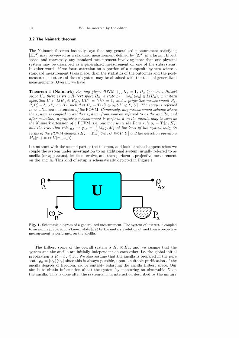
Let us start with the second part of the theorem, and look at what happens when wecouple the system under investigation to an additional system, usually referred to asancilla (or apparatus), let them evolve, and then perform a projective measurementon the ancilla. This kind of setup is schematically depicted in Figure 1.

x

UρA

|ω >B

ρAx

PFig. 1. Schematic diagram of a generalized measurement. The system of interest is coupledto an ancilla prepared in a known state |ωB〉 by the unitary evolution U , and then a projectivemeasurement is performed on the ancilla.

The Hilbert space of the overall system is HA ⊗ HB, and we assume that thesystem and the ancilla are initially independent on each other, i.e. the global initialpreparation is R = %A ⊗ %B. We also assume that the ancilla is prepared in the purestate %B = |ωB〉〈ωB| since this is always possible, upon a suitable purification of theancilla degrees of freedom, i.e. by suitably enlarging the ancilla Hilbert space. Ouraim it to obtain information about the system by measuring an observable X onthe ancilla. This is done after the system-ancilla interaction described by the unitary


operation U . According to the Born rule the probability of the outcomes is given by

px = TrAB

[U%A ⊗ %BU

†I⊗ |x〉〈x|

]= TrA

[%A TrB

[I⊗ %B U

†I⊗ |x〉〈x|U

]︸︷︷︸]

Πx

where the set of operators Πx = TrB

[I⊗ %B U

† I⊗ |x〉〈x|U]

= 〈ωB|U†I⊗PxU |ωB〉 isthe object that would permit to write the Born rule at the level of the subsystem A,i.e. it is our candidate POVM.

In order to prove this, let us define the operators Mx ∈ L(HA) by their action onthe generic vector in HA

Mx|ϕA〉 = 〈x|U |ϕA, ωB〉〉

where |ϕA, ωB〉〉 = |ϕA〉 ⊗ |ωB〉 and the |x〉’s are the orthogonal eigenvectors of X.Using the decomposition of %A =

∑k λk|ψk〉〈ψk| onto its eigenvectors the probability

of the outcomes can be rewritten as

px = TrAB

[U%A ⊗ %BU

†I⊗ |x〉〈x|

]=∑k

λkTrAB

[U |ψk, ωB〉〉〈〈ωB, ψk|U† I⊗ |x〉〈x|

]=∑k

λkTrA

[〈x|U |ψk, ωB〉〉〈〈ωB, ψk|U†|x〉

]=∑k

λkTrA

[Mx|ψk〉〈ψk|M†x

]= TrA

[Mx%AM

†x

]= TrA

[%AM

†xMx

], (6)

which shows that Πx = M†xMx is indeed a positive operator ∀x. Besides, for anyvector |ϕA〉 in HA we have

〈ϕA|∑x

M†xMx|ϕA〉 =∑x

〈〈ωB, ϕA|U†|x〉〈x|U |ϕA, ωB〉〉

= 〈〈ωB, ϕA|U†U |ϕA, ωB〉〉 = 1 , (7)

and since this is true for any |ϕA〉 we have∑xM

†xMx = I. Putting together Eqs. (6)

and (7) we have that the set of operators Πx = M†xMx is a POVM, with detectionoperators Mx. In turn, the conditional state of the system A, after having observedthe outcome x, is given by

%Ax =1

pxTrB

[U%A ⊗ |ωB〉〈ωB|U† I⊗ Px

]=

1

px

∑k

λk〈x|U |ψk, ωB〉〉〈〈ωB, ψk|U†|x〉

=1

pxMx%AM

†x (8)

This is the half of the Naimark theorem: if we couple our system to an ancilla, letthem evolve and perform the measurement of an observable on the ancilla, whichprojects the ancilla on a basis in HB, then this procedure also modify the system.The transformation needs not to be a projection. Rather, it is adequately describedby a set of detection operators which realizes a POVM on the system Hilbert space.Overall, the meaning of the above proof is twofold: on the one hand we have shownthat there exists realistic measurement schemes which are described by POVMs whenwe look at the system only. At the same time, we have shown that the partial trace ofa spectral measure is a POVM, which itself depends on the projective measurementperformed on the ancilla, and on its initial preparation. Finally, we notice that thescheme of Figure 1 provides a general model for any kind of detector with internaldegrees of freedom.


Let us now address the converse problem: given a set of detection operators Mx

which realizes a POVM∑xM

†xMx = I, is this the system-only description of an

indirect measurement performed a larger Hilbert space? In other words, there existsa Hilbert space HB, a state %B = |ωB〉〈ωB| ∈ L(HB), a unitary U ∈ L(HA ⊗ HB),and a projective measurement Px = |x〉〈x| in HB such that Mx|ϕA〉 = 〈x|U |ϕA, ωB〉〉holds for any |ϕA〉 ∈ HA and Πx = 〈ωB|U†I ⊗ PxU |ωB〉? The answer is positive andwe will provide a constructive proof. Let us take HB with dimension equal to thenumber of detection operators and of POVM elements, and choose a basis |x〉 for HB,which in turn individuates a projective measurement. Then we choose an arbitrarystate |ωB〉 ∈ HB and define the action of an operator U as

U |ϕA〉 ⊗ |ωB〉 =∑x

Mx |ϕA〉 ⊗ |x〉

where |ϕA〉 ∈ HA is arbitrary. The operator U preserves the scalar product

〈〈ωB, ϕ′A|U†U |ϕA, ωB〉〉 =

∑xx′

〈ϕ′A|M†x′Mx|ϕA〉〈x′|x〉 =

∑x

〈ϕ′A|M†x′Mx|ϕA〉 = 〈ϕ′A|ϕA〉

and so it is unitary in the one-dimensional subspace spanned by |ωB〉. Besides, itmay be extended to a full unitary operator in the global Hilbert space HA ⊗HB, egit can be the identity operator in the subspace orthogonal to |ωB〉. Finally, for any|ϕA〉 ∈ HA, we have

〈x|U |ϕA, ωB〉〉 =∑x′

Mx′ |ϕA〉〈x|x′〉 = Mx|ϕA〉 ,

and〈ϕA|Πx|ϕA〉 = 〈ϕA|M†xMx|ϕA〉 = 〈〈ωB, ϕA|U†I⊗ PxU |ϕA, ωB〉〉 ,

that is, Πx = 〈ωB|U†I⊗ PxU |ωB〉. utThis completes the proof of the Naimark theorem, which asserts that there is a

one-to-one correspondence between POVM and indirect measurements of the typedescribe above. In other words, an indirect measurement may be seen as the physicalimplementation of a POVM and any POVM may be realized by an indirect measure-ment.

The emerging picture is thus the following: In measuring a quantity of interest ona physical system one generally deals with a larger system that involves additionaldegrees of freedom, besides those of the system itself. These additional physical en-tities are globally referred to as the apparatus or the ancilla. As a matter of fact,the measured quantity may be always described by a standard observable, howeveron a larger Hilbert space describing both the system and the apparatus. When wetrace out the degrees of freedom of the apparatus we are generally left with a POVMrather than a PVM. Conversely, any conceivable POVM, i.e. a set of positive oper-ators providing a resolution of identity, describe a generalized measurement, whichmay be always implemented as a standard measurement in a larger Hilbert space.

Before ending this Section, few remarks are in order:

R1 The possible Naimark extensions are actually infinite, corresponding to the in-tuitive idea that there are infinite ways, with an arbitrary number of ancillarysystems, of measuring a given quantity. The construction reported above is some-times referred to as the canonical extension of a POVM. The Naimark theoremjust says that an implementation in terms of an ancilla-based indirect measure-ment is always possible, but of course the actual implementation may be differentfrom the canonical one.


R2 The projection postulate described at the beginning of this section, the scheme ofindirect measurement, and the canonical extension of a POVM have in commonthe assumption that a nondemolitive detection scheme takes place, in which thesystem after the measurement has been modified, but still exists. This is sometimesreferred to as a measurement of the first kind in textbook quantum mechanics.Conversely, in a demolitive measurement or measurement of the second kind, thesystem is destroyed during the measurement and it makes no sense of speaking ofthe state of the system after the measurement. Notice, however, that for demoli-tive measurements on a field the formalism of generalized measurements providesthe framework for the correct description of the state evolution. As for example,let us consider the detection of photons on a single-mode of the radiation field. Ademolitive photodetector (as those based on the absorption of light) realizes, inideal condition, the measurement of the number operator a†a without leaving anyphoton in the mode . If % =

∑np %np|n〉〈p| is the state of the single-mode radia-

tion field a photodetector of this kind gives a natural number n as output, withprobability pn = %nn, whereas the post-measurement state is the vacuum |0〉〈0|independently on the outcome of the measurement. This kind of measurement isdescribed by the orthogonal POVM Πn = |n〉〈n|, made by the eigenvectors of thenumber operator, and by the detection operator Mn = |0〉〈n|. The proof is left asan exercise.

R3 We have formulated and proved the Naimark theorem in a restricted form, suitablefor our purposes. It should be noticed that it holds in more general terms, as forexample with extension of the Hilbert space given by direct sum rather than tensorproduct, and also relaxing the hypothesis [4].

3.2.1 Conditional states in generalized measurements

If we have a composite system and we perform a projective measurement on,say, subsystem A, the conditional state of the unmeasured subsystem B afterthe observation of the outcome x is given by Eq. (3), i.e. it is the partial traceof the projection of the state before the measurement on the eigenspace of theobserved eigenvalue. One may wonder whether a similar results holds also whenthe measurement performed on the subsystem a A is described by a POVM. Theanswer is positive and the proof may be given in two ways. The first is based onthe observation that, thanks to the existence of a canonical Naimark extension,we may write the state of the global system after the measurement as

%ABx =1

pxMx ⊗ IB %AB M

†x ⊗ IB ,

and thus the conditional state of subsystem B is the partial trace %Bx = TrA[%ABx]i.e.

%Bx =1

pxTrA[Mx⊗IB %AB M

†x⊗IB] =

1

pxTrA[%AB M

†xMx⊗IB] =

1

pxTrA[%AB Πx⊗IB] ,

where again we used the circularity of partial trace in the presence of factorizedoperators. A second proof may be offered invoking the Naimark theorem only toensure the existence of an extension, i.e. a projective measurement on a largerHilbert space HC ⊗ HA, which reduces to the POVM after tracing over HC . Informula, assuming that Px ∈ L(HC⊗ HA) is a projector and σ ∈ L(HC) a density


operator

%Bx =1

pxTrCA [Px ⊗ IB %AB ⊗ σ Px ⊗ IB] =

1

pxTrCA [%AB ⊗ σ Px ⊗ IB]

=1

pxTrA [%ABΠx ⊗ IB] .

3.3 Joint measurement of non commuting observables

A common statement about quantum measurements says that it is not possible toperform a joint measurement of two observables QA and PA of a given system Aif they do not commute, i.e. [QA, PA] 6= 0. This is related to the impossibility offinding any common set of projectors on the Hilbert space HA of the system and todefine a joint observable. On the other hand, a question arises on whether commonprojectors may be found in a larger Hilbert space, i.e. whether one may implement ajoint measurement in the form of a generalized measurement. The answer is indeedpositive [5,6]: This Section is devoted to describe the canonical implementation of jointmeasurements for pair of observables having a (nonzero) commutator [QA, PA] = c I 6=0 proportional to the identity operator.

The basic idea is to look for a pair of commuting observables [XAB, YAB] = 0 in alarger Hilbert space HA⊗HB which trace the observables PA and QA, i.e. which havethe same expectation values

〈XAB〉 ≡ TrAB[XAB %A ⊗ %B] = TrA[QA %A] ≡ 〈QA〉〈YAB〉 ≡ TrAB[YAB %A ⊗ %B] = TrA[PA %A] ≡ 〈PA〉 (9)

for any state %A ∈ HA of the system under investigation, and a fixed suitable prepa-ration %B ∈ HB of the system B. A pair of such observables may be found uponchoosing a replica system B, identical to A, and considering the operators

XAB = QA ⊗ IB + IA ⊗QB

YAB = PA ⊗ IB − IA ⊗ PB (10)

where QB and PB are the analogue of QA and PA for system B, see [7] for more detailsinvolving the requirement of covariance. The operators in Eq. (10), taken together astate %B ∈ HB satisfying

TrB[QB %B] = TrB[PB %B] = 0 , (11)

fulfill the conditions in Eq. (9), i.e. realize a joint generalized measurement of thenoncommuting observables QA and PA. The operators XAB and YAB are Hermitian byconstruction. Their commutator is given by

[XAB, YAB] = [QA, PA]⊗ IB − IA ⊗ [QB, PB] = 0 . (12)

Notice that the last equality, i.e. the fact that the two operators commute, is validonly if the commutator [QA, PA] = c I is proportional to the identity. More generalconstructions are needed if this condition does not hold [8].

Since the [XAB, YAB] = 0 the complex operator ZAB = XAB + i YAB is normal i.e.

[ZAB, Z†AB] = 0. For normal operators the spectral theorem holds, and we may write

ZAB =∑z

z Pz Pz = |z〉〉〈〈z| ZAB|z〉〉 = z|z〉〉 (13)


where z ∈ C, and Pz are orthogonal projectors on the eigenstates |z〉〉 ≡ |z〉〉AB of ZAB.The set {Pz} represents the common projectors individuating the joint observableZAB. Each run of the measurement returns a complex number, whose real and imag-inary parts correspond to a sample of the XAB and YAB values, aiming at samplingQA and PA. The statistics of the measurement is given by

pZ(z) = TrAB[%A ⊗ %B Pz] = TrA[%AΠz] (14)

where the POVM Πz is given by

Πz = TrB[IA ⊗ %B Pz] . (15)

The mean values 〈XAB〉 = 〈QA〉 and 〈YAB〉 = 〈PA〉 are the correct ones by construction,where by saying ”correct” we intend the mean values that one would have recorded bymeasuring the two observables QA and PA separately in a standard (single) projectivemeasurement on %A. On the other hand, the two marginal distributions

pX(x) =

∫dy pZ(x+ iy) pY (y) =

∫dx pZ(x+ iy) ,

need not to reproduce the distributions obtained in single measurements. In particu-lar, for the measured variances 〈∆X2

AB〉 = 〈X2AB〉 − 〈XAB〉2 and 〈∆YAB〉 one obtains

〈∆X2AB〉 = Tr

[(Q2

A ⊗ IB + IA ⊗Q2B + 2QA ⊗QB) %A ⊗ %B

]− 〈QA〉2

= 〈∆Q2A〉+ 〈Q2

B〉〈∆Y 2

AB〉 = 〈∆P 2A〉+ 〈P 2

B〉 (16)

where we have already taken into account that 〈QB〉 = 〈PB〉 = 0. As it is apparentfrom Eqs. (16) the variances of XAB and YAB are larger than those of the original, noncommuting, observables QA and PA.

Overall, we may summarize the emerging picture as follows: a joint measurementof a pair of non commuting observables corresponds to a generalized measurementand may be implemented as the measurement of a pair of commuting observables onan enlarged Hilbert space. Mean values are preserved whereas the non commutingnature of the original observables manifests itself in the broadening of the marginaldistributions, i.e. as an additional noise term appears to both the variances. Theuncertainty product may be written as

〈∆X2AB〉〈∆Y 2

AB〉 = 〈∆Q2A〉〈∆P 2

A〉+ 〈∆Q2A〉〈P 2

B〉+ 〈Q2B〉〈∆P 2

A〉+ 〈Q2B〉〈P 2

B〉 ,

≥ 1

4

∣∣[QA, PA]∣∣2 + 〈∆Q2

A〉〈P 2B〉+ 〈Q2

B〉〈∆P 2A〉+ 〈Q2

B〉〈P 2B〉 , (17)

where the last three terms are usually referred to as the added noise due to the jointmeasurement. If we perform a joint measurement on a minimum uncertainty state(MUS, see Appendix B) for a given pair of observables (e.g. a coherent state in thejoint measurement of a pair of conjugated quadratures of the radiation field) and usea MUS also for the preparation of the replica system (e.g. the vacuum), then Eq. (17)rewrites as

〈∆X2AB〉〈∆Y 2

AB〉 =∣∣[QA, PA]

∣∣2 . (18)

This is four times the minimum attainable uncertainty product in the case of a mea-surement of a single observable (see Appendix B). In terms of rms’ ∆X =

√〈∆X2〉

we have a factor 2, which is usually referred to as the 3 dB of added noise in jointmeasurements. The experimental realization of joint measurements of non commutingobservables has been carried out for conjugated quadratures of the radiation field ina wide range of frequencies ranging from radiowaves to the optical domain, see e.g.[9].


3.4 About the so-called Heisenberg principle

Let us start by quoting Wikipedia about the Heisenberg principle [10]

Published by Werner Heisenberg in 1927, the principle implies that it is impos-sible to simultaneously both measure the present position while ”determining”the future momentum of an electron or any other particle with an arbitrarydegree of accuracy and certainty. This is not a statement about researchers’ability to measure one quantity while determining the other quantity. Rather,it is a statement about the laws of physics. That is, a system cannot be de-fined to simultaneously measure one value while determining the future valueof these pairs of quantities. The principle states that a minimum exists for theproduct of the uncertainties in these properties that is equal to or greater thanone half of the reduced Planck constant.

As is it apparent from the above formulation, the principle is about the precisionachievable in the measurement of an observable and the disturbance introduced by thesame measurement on the state under investigation, which, in turn, would limit theprecision of a subsequent measurement of the conjugated observable. The principle,which has been quite useful in the historical development of quantum mechanics, hasbeen inferred from the analysis of the celebrated Heisenberg’ gedanken experiments,and thus is heuristic in nature. However, since its mathematical formulation is relatedto that of the uncertainty relations (see Appendix B), it is often though as a theoremfollowing from the axiomatic structure of quantum mechanics. This is not the case:here we exploit the formalism of generalized measurements to provide an explicitexample of a measurement scheme providing the maximum information about a givenobservable, i.e. the statistics of the corresponding PVM, while leaving the state underinvestigation in an eigenstate of the conjugated observable.

Let us consider the two noncommuting observables [A,B] = c I and the set ofdetection operators Ma = |b〉〈a| where |a〉 and |b〉 are eigenstates of A and B respec-tively, i.e. A|a〉 = a|a〉, B|b〉 = b|b〉. According to the Naimark theorem the set ofoperators {Ma} describe a generalized measurement (e.g. an indirect measurementas the one depicted in Fig. 1) with statistics pa = Tr[%Πa] described by the POVMΠa = M†aMa = |a〉〈a| and where the conditional states after the measurement aregiven by %a = 1

paMa%M

†a = |b〉〈b|. In other words, the generalized measurement

described by the set {Ma} has the same statistics of a Von-Neumann projective mea-surement of the observable A, and leave the system under investigating in an eigen-state of the observable B, thus determining its future value with an arbitrary degreeof accuracy and certainty and contrasting the formulation of the so-called Heisenbergprinciple reported above. An explicit unitary realization of this kind of measurementfor the case of position, as well as a detailed discussion on the exact meaning ofthe Heisenberg principle, and the tradeoff between precision and disturbance in aquantum measurement, may be found in [11].

3.5 The quantum roulette

Let us considerK projective measurements corresponding toK nondegenerate isospec-tral observables Xk, k = 1, ...,K in a Hilbert space H, and consider the followingexperiment. The system is sent to a detector which at random, with probabilityzk,∑k zk = 1, perform the measurement of the observable Xk. This is known as the

quantum roulette since the observable to be measured is chosen at random, eg accord-ing to the outcome of a random generator like a roulette. The probability of gettingthe outcome x from the measurement of the observable Xk on a state % ∈ L(H) is


given by p(k)x = Tr[%P

(k)x ], P

(k)x = |x〉kk〈x|, and the overall probability of getting the

outcome x from our experiment is given by

px =∑k

zkp(k)x =

∑k

zkTr[%P (k)x ] = Tr[%

∑k

zkP(k)x ] = Tr[%Πx] ,

where the POVM describing the measurement is given by Πx =∑k zkP

(k)x . This is

indeed a POVM and not a projective measurement since

ΠxΠx′ =∑kk′

zkzk′P(k)x P

(k′)x′ 6= δxx′Πx .

Again, we have a practical situation where POVMs naturally arise in order to describethe statistics of the measurement in terms of the Born rule and the system densityoperator. A Naimark extension for the quantum roulette may be obtained as follows.Let us consider an additional probe system described by the Hilbert space HP ofdimension K equal to the number of measured observables in the roulette, and the

set of projectors Qx =∑k P

(k)x ⊗ |θk〉〈θk| where {|θk〉} is a basis for HP . Then, upon

preparing the probe system in the superposition |ωP 〉 =∑k

√zk|θk〉 we have that

px = TrSP [% ⊗ |ωP 〉〈ωP |Qx] and, in turn, Πx = TrP [IS ⊗ |ωP 〉〈ωP |Qx] =∑k zkP

(k)x .

The state of the system after the measurement may be obtained as the partial trace

%x =1

pxTrP [Qx %⊗ |ωP 〉〈ωP |Qx]

=1

px

∑k

∑k′

TrP

[P (k)x ⊗ |θk〉〈θk| %⊗ |ωP 〉〈ωP |P (k′)

x ⊗ |θk′〉〈θk′ |]

=1

px

∑k

zkP(k)x %P (k)

x .

Notice that the presented Naimark extension is not the canonical one.

Exercise 7 Prove that the operators Qx introduced for the Naimark extension ofthe quantum roulette, are indeed projectors.

Exercise 8 Take a system made by a single qubit system and construct the canonicalNaimark extension for the quantum roulette obtained by measuring the observablesσα = cosασ1 + sinασ2, where σ1 and σ2 are Pauli matrices and α ∈ [0, π] is chosenat random with probability density p(α) = π−1.

4 Quantum operations

In this Section we address the dynamical evolution of quantum systems to see whetherthe standard formulation in terms of unitary evolutions needs a suitable generaliza-tion. This is indeed the case: we will introduce a generalized description and see howthis reconciles with what we call Postulate 3 in the Introduction. We will proceedin close analogy with what we have done for states and measurements. We start byclosely inspecting the physical motivations behind any mathematical description ofquantum evolution, and look for physically motivated conditions that a map, intendedto transform a quantum state into a quantum state, from now on a quantum operation,should satisfy to be admissible. This will lead us to the concept of complete positivity,which suitably generalizes the motivations behind unitarity. We then prove that any


quantum operation may be seen as the partial trace of a unitary evolution in a largerHilbert space, and illustrate a convenient form, the so-called Kraus or operator-sumrepresentation, to express the action of a quantum operation on quantum states.

By quantum operation we mean a map %→ E(%) transforming a quantum state %into another quantum state E(%). The basic requirements on E to describe a physicallyadmissible operations are those captured by the request of unitarity in the standardformulation, i.e.

Q1 The map is positive and trace-preserving, i.e. E(%) ≥ 0 (hence selfadjoint) andTr[E(%)] = Tr[%] = 1. The last assumption may be relaxed to that of being tracenon-increasing 0 ≤ Tr[E(%)] ≤ 1 in order to include evolution induced by mea-surements (see below).

Q2 The map is linear E(∑k pk%k) =

∑k pkE(%k), i.e. the state obtained by applying

the map to the ensemble {pk, %k} is the ensemble {pk, E(%k)}.Q3 The map is completely positive (CP), i.e. besides being positive it is such that if we

introduce an additional system, any map of the form E ⊗I acting on the extendedHilbert space is also positive. In other words, we ask that the map is physicallymeaningful also when acting on a portion of a larger, composite, system. As wewill see, this request is not trivial at all, i.e. there exist maps that are positive butnot completely positive.

4.1 The operator-sum representation

This section is devoted to state and prove a theorem showing that a map is a quantumoperation if and only if it is the partial trace of a unitary evolution in a larger Hilbertspace, and provides a convenient form, the so-called Kraus decomposition or operator-sum representation [12,13], to express its action on quantum states.

Theorem 5 (Kraus) A map E is a quantum operation i.e. it satisfies the require-ments Q1-Q3 if and only if is the partial trace of a unitary evolution on a largerHilbert space with factorized initial condition or, equivalently, it possesses a Kraus

decomposition i. e. its action may be represented as E(%) =∑kMk%M

†k where {Mk}

is a set of operators satisfying∑kM

†kMk = I.

Proof The first part of the theorem consists in assuming that E(%) is the partial traceof a unitary operation in a larger Hilbert space and prove that it has a Kraus decom-position and, in turn, it satisfies the requirements Q1-Q3. Let us consider a physicalsystem A prepared in the quantum state %A and another system B prepared in thestate %B. A and B interact through the unitary operation U and we are interestedin describing the effect of this interaction on the system A only, i.e. we are lookingfor the expression of the mapping %A → %′A = E(%A) induced by the interaction. Thismay be obtained by performing the partial trace over the system B of the global ABsystem after the interaction, in formula

E(%A) = TrB

[U %A ⊗ %BU

†] =∑s

psTrB

[U %A ⊗ |θs〉〈θs|U†

]=∑st

ps〈ϕt|U |θs〉 %A〈θs|U†|ϕt〉 =∑k

Mk %AM†k (19)

where we have introduced the operatorMk =√ps〈ϕt|U |θs〉, with the polyindex k ≡ st

obtained by a suitable ordering, and used the spectral decomposition of the densityoperator %B =

∑s ps|θs〉〈θs|. Actually, we could have also assumed the additional

system in a pure state |ωB〉, since this is always possible upon invoking a purification,


i.e. by suitably enlarging the Hilbert space. In this case the elements in the Krausdecomposition of our map would have be written as 〈ϕt|U |ωB〉. The set of operators{Mk} satisfies the relation∑

k

M†Mk =∑st

psθs|U†|ϕt〉〈ϕt|U |θs〉 =∑s

ps〈θs|U†U |θs〉 = I .

Notice that the assumption of a factorized initial state is crucial to prove the existenceof a Kraus decomposition and, in turn, the complete positivity. In fact, the dynamicalmap E(%A) = TrB

[U %AB U

†] resulting from the partial trace of an initially correlatedpreparation %AB needs not to be so. In this case, the dynamics can properly be definedonly on a subset of initial states of the system. Of course, the map can be extendedto all possible initial states by linearity, but the extension may not be physicallyrealizable, i.e. may be not completely positive or even positive [14].

We now proceed to show that for map of the form (19) (Kraus decomposition) theproperties Q1-Q3 hold. Preservation of trace and of the Hermitian character, as wellas linearity, are guaranteed by the very form of the map. Positivity is also ensured,since for any positive operator OA ∈ L(HA) and any vector |ϕA〉 ∈ HA we have

〈ϕA|E(OA)|ϕA〉 = 〈ϕA|∑k

Mk OAM†k |ϕA〉 = 〈ϕA|TrB[U OA ⊗ %B U

†]|ϕA〉

= TrAB[U†|ϕA〉〈ϕA| ⊗ IU OA ⊗ %B ] ≥ 0 ∀OA,∀ %B,∀ |ϕA〉 .

Therefore it remains to be proved that the map is completely positive. To this aimlet us consider a positive operator OAC ∈ L(HA ⊗HC) and a generic state |ψAC〉〉 onthe same enlarged space, and define

|ωk〉〉 =1√Nk

Mk ⊗ IC |ψAC〉〉 Nk = 〈〈ψAC |M†kMk ⊗ IC |ψAC〉〉 ≥ 0 .

Since OAC is positive we have

〈〈ψAC |(M†k ⊗ IC)OAC(Mk ⊗ IC)|ψAC〉〉 = Nk〈〈ωk|OAC |ωk〉〉 ≥ 0

and therefore 〈〈ψAC |E ⊗ IC(OAC)|ψAC〉〉 =∑kNk〈〈ωk|OAC |ωk〉〉 ≥ 0, which proves

that for any positive OAC also E ⊗ IC(OAC) is positive for any choice of HC , i.e. E isa CP-map.

Let us now prove the second part of the theorem, i.e. we consider a map E :L(HA)→ L(HA) satisfying the requirements Q1-Q3 and show that it may be writtenin the Kraus form and, in turn, that its action may be obtained as the partial traceof a unitary evolution in a larger Hilbert. We start by considering the state |ϕ〉〉 =1√d

∑k |θk〉⊗|θk〉 ∈ HA⊗HA and define the operator %AA = E ⊗I(|ϕ〉〉〈〈ϕ|). From the

complete positivity and trace preserving properties of E we have that Tr[%AA] = 1,and %AA ≥ 0, i.e. %AA is a density operator. Besides, this establishes a one-to-onecorrespondence between maps L(HA) → L(HA) and density operators in L(HA) ⊗L(HA) which may be proved as follows: for any |ψ〉 =

∑k ψk|θk〉 ∈ HA define |ψ〉 =∑

k ψ∗k|θk〉 and notice that

〈ψ|%AA|ψ〉 =1

d〈ψ|∑kl

E(|θk〉〈θl|)⊗|θk〉〈θl| |ψ〉 =1

d

∑kl

ψ∗l ψk E(|θk〉〈θl|) =1

dE(|ψ〉〈ψ|) ,

where we used linearity to obtain the last equality. Then define the operators Mk|ψ〉 =√dpk〈ψ|ωk〉〉, where |ωk〉〉 are the eigenvectors of %AA =

∑k pk|ωk〉〉〈〈ωk|: this is a


linear operator on HA and we have∑k

Mk|ψ〉〈ψ|M†k = d∑k

pk〈ψ|ωk〉〉〈〈ωk|ψ〉 = d〈ψ|%AA|ψ〉 = E(|ψ〉〈ψ|)

for all pure states. Using again linearity we have that E(%) =∑kMk%M

†k also for

any mixed state. It remains to be proved that a unitary extension exists, i.e. toprove that for any map on L(HA) which satisfies Q1-Q3, and thus possesses a Krausdecomposition, there exist: i) a Hilbert space HB, ii) a state |ωB〉 ∈ HB, iii) a unitaryU ∈ L(HA ⊗HB) such that E(%A) = TrB[U %A ⊗ |ωB〉〈ωB|U†] for any %A ∈ L(HA). Tothis aim we proceed as we did for the proof of the Naimark theorem, i.e. we take anarbitrary state |ωB〉 ∈ HB, and define an operator U trough its action on the genericϕA〉 ⊗ |ωB〉 ∈ HA ⊗ HB, U |ϕA〉 ⊗ |ωB〉 =

∑kMk |ϕA〉 ⊗ |θk〉, where the |θk〉’s are a

basis for HB. The operator U preserves the scalar product

〈〈ωB, ϕ′A|U†U |ϕA, ωB〉〉 =

∑kk′

〈ϕ′A|M†k′Mk|ϕA〉〈θk′ |θk〉 =

∑k

〈ϕ′A|M†kMk|ϕA〉 = 〈ϕ′A|ϕA〉

and so it is unitary in the one-dimensional subspace spanned by |ωB〉. Besides, it maybe extended to a full unitary operator in the global Hilbert space HA⊗HB, eg it canbe the identity operator in the subspace orthogonal to |ωB〉. Then, for any %A in HA

we have

TrB

[U%A ⊗ |ωB〉〈ωB|U†

]=∑s

ps TrB

[U |ψs〉〈ψs| ⊗ |ωB〉〈ωB|U†

]=∑skk′

ps TrB

[Mk|ψs〉〈ψs|M†k′ ⊗ |θk〉〈θk′ |

]=∑sk

psMk|ψs〉〈ψs|M†k =∑k

Mk%AM†k ut

The Kraus decomposition of a quantum operation generalizes the unitary descriptionof quantum evolution. Unitary maps are, of course, included and correspond to mapswhose Kraus decomposition contains a single elements. The set of quantum operationsconstitutes a semigroup, i.e. the composition of two quantum operations is still aquantum operation:

E2(E1(%)) =∑k1

M(1)k1E2(%)M

(1)†k1

=∑k1k2

M(1)k1M

(2)k2%M

(2)†k2

M(1)†k1

=∑k

Mk%M†k ,

where we have introduced the polyindex k. Normalization is easily proved, since∑k M

†kMk =

∑k1k2

M(2)†k2

M(1)†k1

M(1)k1M

(2)k2

= I. On the other hand, the existence of

inverse is not guaranteed: actually only unitary operations are invertible (with a CPinverse).

The Kraus theorem also allows us to have a unified picture of quantum evolution,either due to an interaction or to a measurement. In fact, the modification of the state

in the both processes is described by a set of operators Mk satisfying∑kM

†kMk = I.

In this framework, the Kraus operators of a measurement are what we have referredto as the detection operators of a POVM.

4.1.1 The dual map and the unitary equivalence

Upon writing the generic expectation value for the evolved state E(%) and exploitingboth linearity and circularity of trace we have

〈X〉 = Tr[E(%)X] =∑k

Tr[Mk%M†k X] =

∑k

Tr[%M†kXMk] = Tr[%E∨(X)] ,


where we have defined the dual map E∨(X) =∑kM

†kXMk which represents the

”Heisenberg picture” for quantum operations. Notice also that the elements of theKraus decomposition Mk = 〈ϕk|U |ωB〉 depend on the choice of the basis used toperform the partial trace. Change of basis cannot have a physical effect and thismeans that the set of operators

Nk = 〈θk|U |ωB〉 =∑s

〈θk|ϕs〉〈ϕs|U |ωB〉 =∑s

VksMs ,

where the unitary V ∈ L(HB) describes the change of basis, and the original set Mk

actually describe the same quantum operations, i.e.∑kNk%N

†k =

∑kMk%M

†k , ∀%.

The same can be easily proved for the system B prepared in mixed state. The originof this degree of freedom stays in the fact that if the unitary U on HA ⊗ HB andthe state |ωB〉 ∈ HB realize an extension for the map E : L(HA) → L(HA) then anyunitary of the form (I⊗V )U is a unitary extension too, with the same ancilla state. Aquantum operation is thus identified by an equivalence class of Kraus decompositions.An interesting corollary is that any quantum operation on a given Hilbert space ofdimension d may be generated by a Kraus decomposition containing at most d2 ele-

ments, i.e. given a Kraus decomposition E(%) =∑kMk%M

†k with an arbitrary number

of elements, one may exploit the unitary equivalence and find another representation

E(%) =∑kNk%N

†k with at most d2 elements.

4.2 The random unitary map and the depolarizing channel

A simple example of quantum operation is the random unitary map, defined by the

Kraus decomposition E(%) =∑k pkUk%U

†k , i.e. Mk =

√pk Uk and U†kUk = I. This

map may be seen as the evolution resulting from the interaction of our system withanother system of dimension equal to the number of elements in the Kraus decompo-sition of the map via the unitary V defined by V |ψA〉⊗ |ωB〉 =

∑k

√pk Uk|ψA〉⊗ |θk〉,

|θk〉 being a basis for HB which includes |ωB〉. If ”we do not look” at the systemB and trace out its degree of freedom the evolution of system A is governed by therandom unitary map introduced above.

Exercise 9 Prove explicitly the unitarity of V.

The operator-sum representation of quantum evolutions have been introduced, andfinds its natural application, for the description of propagation in noisy channels, i.e.the evolution resulting from the interaction of the system of interest with an externalenvironment, which generally introduces noise in the system degrading its coherence.As for example, let us consider a qubit system (say, the polarization of a photon), onwhich we have encoded binary information according to a suitable coding procedure,traveling from a sender to a receiver. The propagation needs a physical support (say,an optical fiber) and this unavoidably leads to consider possible perturbations toour qubit, due to the interaction with the environment. The resulting open systemdynamics is usually governed by a Master equation, i.e. the equation obtained bypartially tracing the Schroedinger (Von Neumann) equation governing the dynamicsof the global system, and the solution is expressed in form of a CP-map. For a qubitQ in a noisy environment a quite general description of the detrimental effects of theenvironment is the so-called depolarizing channel [1], which is described by the Kraus

operator M0 =√

1− γ σ0, Mk =√γ/3σk, k = 1, 2, 3, i.e.

E(%) = (1− γ)%+γ

3

∑k

σk % σk 0 ≤ γ ≤ 1 .


The depolarizing channel may be seen as the evolution of the qubit due to the inter-action with a four-dimensional system through the unitary

V |ψQ〉 ⊗ |ωE〉 =√

1− γ|ψQ〉 ⊗ |ωE〉+

√γ

3

3∑k=1

σk|ψQ〉 ⊗ |θk〉 ,

|θk〉 being a basis which includes |ωE〉. From the practical point view, the map de-scribes a situation in which, independently on the underlying physical mechanism, wehave a probability γ/3 that a perturbation described by a Pauli matrix is applied tothe qubit. If we apply σ1 we have the so-called spin-flip i.e. the exchange |0〉 ↔ |1〉,whereas if we apply σ3 we have the phase-flip, and for σ2 we have a specific combi-nation of the two effects. Since for any state of a qubit %+

∑k σk%σk = 2I the action

of the depolarizing channel may be written as

E(%) = (1− γ)%+γ

3(2I− %) =

2

3γI+ (1− 4

3γ)% = p%+ (1− p)I

2,

where p = 1− 43γ, i.e. − 1

3 ≤ p ≤ 1. In other words, we have that the original state % is

sent to a linear combination of itself and the maximally mixed state I

2 , also referredto as the depolarized state.

Exercise 10 Express the generic qubit state in Bloch representation and explicitlywrite the effect of the depolarizing channel on the Bloch vector.

Exercise 11 Show that the purity of a qubit cannot increase under the action of thedepolarizing channel.

4.3 Transposition and partial transposition

The transpose T (X) = XT of an operator X is the conjugate of its adjoint XT =(X†)∗ = (X∗)†. Upon the choice of a basis we have X =

∑nkXnk|θn〉〈θk| and

thus XT =∑nkXnk|θk〉〈θn| =

∑nkXkn|θn〉〈θk|. Transposition does not change the

trace of an operator, neither its eigenvalues. Thus it transforms density operatorsinto density operators: Tr[%] = Tr[%T ] = 1 %T ≥ 0 if % ≥ 0. As a positive, tracepreserving, map it is a candidate to be a quantum operation. On the other hand,we will show by a counterexample that it fails to be completely positive and thus itdoes not correspond to physically admissible quantum operation. Let us consider abipartite system formed by two qubits prepared in the state |ϕ〉〉 = 1√

2|00〉〉+ |11〉〉.

We denote by %τ = I⊗ T (%) the partial transpose of % i.e. the operator obtained bythe application of the transposition map to one of the two qubits. We have

(|ϕ〉〉〈〈ϕ|

)τ=

1

2

1 0 0 10 0 0 00 0 0 01 0 0 1

τ

=1

2

(|0〉〈0| ⊗ |0〉〈0|+ |1〉〈1| ⊗ |1〉〈1|+ |0〉〈1| ⊗ |0〉〈1|+ |1〉〈0| ⊗ |1〉〈0|

)τ=

1

2

(|0〉〈0| ⊗ |0〉〈0|+ |1〉〈1| ⊗ |1〉〈1|+ |0〉〈1| ⊗ |1〉〈0|+ |1〉〈0| ⊗ |0〉〈1|

)

=1

2

1 0 0 00 0 1 00 1 0 00 0 0 1


Using the last expression it is straightforward to evaluate the eigenvalues of %τ , whichare + 1

2 (multiplicity three) and − 12 . In other words I⊗ T is not a positive map and

the transposition is not completely positive. Notice that for a factorized state of theform %AB = %A ⊗ %B we have I ⊗ T (%AB) = %A ⊗ %T

B ≥ 0 i.e. partial transpositionpreserves positivity in this case .

Exercise 12 Prove that transposition is not a CP-map by its action on any stateof the form |ϕ〉〉 = 1√

d

∑k |ϕk〉 ⊗ |θk〉. Hint: the operator I ⊗ T (|ϕ〉〉〈〈ϕ|) ≡ E is the

so-called swap operator since it ”exchanges” states as E(|ψ〉A ⊗ |ϕ〉B) = |ϕ〉A ⊗ |ψ〉B.

5 Conclusions

In this tutorial, we have addressed the postulates of quantum mechanics about states,measurements and operations. We have reviewed their modern formulation and intro-duced the basic mathematical tools: density operators, POVMs, detection operatorsand CP-maps. We have shown how they provide a suitable framework to describequantum systems in interaction with their environment, and with any kind of mea-suring and processing devices. The connection with the standard formulation havebeen investigated in details building upon the concept of purification and the Theo-rems of Naimark and Stinespring/Kraus-Choi-Sudarshan.

The framework and the tools illustrated in this tutorial are suitable for the pur-poses of quantum information science and technology, a field which has fostered newexperiments and novel views on the conceptual foundation of quantum mechanics,but has so far little impact on the way that it is taught. We hope to contribute indisseminating these notions to a larger audience, in the belief that they are useful forseveral other fields, from condensed matter physics to quantum biology.

I’m grateful to Konrad Banaszek, Alberto Barchielli, Maria Bondani, Mauro D’Ariano, IvoP. Degiovanni, Marco Genoni, Marco Genovese, Paolo Giorda, Chiara Macchiavello, SabrinaManiscalco, Alex Monras, Stefano Olivares, Jyrki Piilo, Alberto Porzio, Massimiliano Sacchi,Ole Steuernagel, and Bassano Vacchini for the interesting and fruitful discussions aboutfoundations of quantum mechanics and quantum optics over the years. I would also liketo thank Gerardo Adesso, Alessandra Andreoni, Rodolfo Bonifacio, Ilario Boscolo, VladoBuzek, Berge Englert, Zdenek Hradil, Fabrizio Illuminati, Ludovico Lanz, Luigi Lugiato,Paolo Mataloni, Mauro Paternostro, Mladen Pavicic, Francesco Ragusa, Mario Rasetti, MikeRaymer, Jarda Rehacek, Salvatore Solimeno, and Paolo Tombesi.

References

1. M. Nielsen, E. Chuang, Quantum Computation and Quantum Information, (CambridgeUniversity Press, 2000).

2. A. Peres, Quantum Theory: concepts and methods, (Kluwer Academic, Dordrecht, 1993).3. J. Bergou, J. Mod. Opt. 57, 160 (2010).4. V. Paulsen, Completely Bounded Maps and Operator Algebras (Cambridge University

Press, 2003).5. E. Arthurs, J. L. Kelly, Bell. Syst. Tech. J. 44, 725 (1965); J. P. Gordon, W. H. Louisell in

Physics of Quantum Electronics (Mc-Graw-Hill, NY, 1966); E. Arthurs, M. S. Goodman,Phys. Rev. Lett. 60, 2447 (1988).

6. H. P. Yuen, Phys. Lett. A 91, 101 (1982).7. B. Vacchini in Theoretical foundations of quantum information processing and commu-

nication, E. Bruening et al (Eds.), Lect. Not. Phys. 787, 39 (2010).


8. E. Prugovecki, J. Phys. A 10, 543 (1977).9. N. G. Walker, J. E. Carrol, Opt. Quantum Electr. 18, 355 (1986); N. G. Walker, J. Mod.

Opt. 34, 16 (1987).10. \protect\vrule width0pt\protect\href{http://en.wikipedia.org/wiki/Uncertainty_principle}{http://en.wikipedia.org/wiki/Uncertainty_principle}11. M. Ozawa, Phys. Lett. A 299, 17 (2002); Phys. Rev. A 67, 042105 (2003); J. Opt. B 7,

S672 (2005).12. J. Preskill, Lectures notes for Physics 229: Quantum information and computation avail-

able at www.theory.caltech.edu/ preskill/ph229/13. Depending on the source, and on the context, the theorem is known as the Stinespring

dilation theorem, or the Kraus-Choi-Sudarshan theorem.14. P. Pechukas, Phys. Rev. Lett. 73, 1060 (1994).15. R. Puri, Mathematical methods of quantum optics (Springer, Berlin, 2001).16. K. E. Cahill, R. J. Glauber, Phys. Rev. 177, 1857 (1969); 177, 1882 (1969).

Further readings

1. I. Bengtsson, K. Zyczkowski, Geometry of Quantum States, (Cambridge University Press,2006).

2. Lectures and reports by C. M. Caves, available at http://info.phys.unm.edu/ caves/3. P. Busch, M. Grabowski, P. J. Lahti,Operational Quantum Mechanics, Lect. Notes. Phys.

31, (Springer, Berlin,1995).4. T. Heinosaari, M. Ziman, Acta Phys. Slovaca 58, 487 (2008).5. C. W. Helstrom, Quantum Detection and Estimation Theory (Academic Press, New York,

1976)6. A.S. Holevo, Statistical Structure of Quantum Theory, Lect. Not. Phys 61, (Springer,

Berlin, 2001).7. M. Ozawa, J. Math. Phys. 25, 79 (1984).8. M. G. A. Paris, J. Rehacek (Eds.), Quantum State Estimation Lect. Notes Phys. 649,

(Springer, Berlin, 2004).9. V. Gorini, A. Frigerio, M. Verri, A. Kossakowski, E. C. G. Sudarshan, Rep. Math. Phys.

13, 149 (1978).10. F. Buscemi, G. M. D’Ariano, and M. F. Sacchi, Phys. Rev. A 68. 042113 (2003).11. K. Banaszek, Phys. Rev. Lett. 86, 1366 (2001).

A Trace and partial trace

The trace of an operator O is a scalar quantity equal to sum of diagonal elements in agiven basis Tr[O] =

∑n〈ϕn|O|ϕn〉. The trace is invariant under any change of basis,

as it is proved by the following chain of equalities∑n

〈θn|O|θn〉 =∑njk

〈θn|ϕk〉〈ϕk|O|ϕj〉〈ϕj |θn〉 =∑njk

〈ϕj |θn〉〈θn|ϕk〉〈ϕk|O|ϕj〉

=∑jk

〈ϕj |ϕk〉〈ϕk|O|ϕj〉 =∑k

〈ϕk|O|ϕk〉 ,

where we have suitably inserted and removed resolutions of the identity in terms ofboth basis {|θn〉} and {|ϕn〉}. As a consequence, using the basis of eigenvectors ofO, Tr[O] =

∑n on, on being the eigenvalues of O. Trace is a linear operation, i.e.

Tr[O1 + O2] = Tr[O1] + Tr[O2] and Tr[λO] = λTr[O] and thus ∂Tr[O] = Tr[∂O] forany derivation. The trace of any ”ket-bra” Tr[|ψ1〉〈ψ2|] is obtained by ”closing thesandwich” Tr[|ψ1〉〈ψ2|] = 〈ψ2|ψ1〉; in fact upon expanding the two vectors in the samebasis and taking the trace in that basis Tr[|ψ1〉〈ψ2|] =

∑nkl ψ1kψ

∗2l〈θn|θk〉〈θl|θn〉 =∑

n ψ1nψ∗2n = 〈ψ2|ψ1〉. Other properties are summarized by the following theorem.

http://info.phys.unm.edu/


Theorem 6 For the trace operation the following properties hold

i) Given any pair of operators Tr[A1A2] = Tr[A2A1]ii) Given any set of operators A1, ..., AN we Tr[A1A2A3...AN ] = Tr[A2A3...ANA1] =

Tr[A3A4...A1A2] = ... (circularity).

Proof : left as an exercise. ut

Notice that the ”circularity” condition is essential to have property ii) i.e. Tr[A1A2A3] =Tr[A2A3A1], but Tr[A1A2A3] 6= Tr[A2A1A3]

Partial traces RB ∈ L(HB) RA ∈ L(HA) of an operator R in L(H1 ⊗ H2) aredefined accordingly as

RB = TrA [R ] =∑n

A〈ϕn|R |ϕn〉A RA = TrB [R ] =∑n

B〈ϕn|R |ϕn〉B

and circularity holds only for single-system operators, e.g., if R1, R2 ∈ L(HA ⊗HB),A ∈ L(HA), B ∈ L(HB)

TrA [A⊗ IR1R2] =∑n

an〈an|R1R2|an〉 = TrA [R1R2A⊗ I]

TrA [A⊗BR1R2] =∑n

an〈an|I⊗BR1R2|an〉 = TrA [I⊗BR1R2A⊗ I]

6=∑n

an〈an|R1R2 I⊗B|an〉 = TrA [R1R2A⊗B]

Exercise 13 Consider a generic mixed state % ∈ L(H ⊗ H) and write the matrixelements of the two partial traces in terms of the matrix elements of %.

Exercise 14 Prove that also partial trace is invariant under change of basis.

B Uncertainty relations

Two non commuting observables [X,Y ] 6= 0 do not admit a complete set of commoneigenvectors, and thus it not possible to find common eigenprojectors and to definea joint observable. Two non commuting observables are said to be incompatible orcomplementary, since they cannot assume definite values simultaneously. A strikingconsequence of this fact is that when we measure an observable X the precision ofthe measurement, as quantified by the variance 〈∆X2〉 = 〈X2〉 − 〈X〉2, is influencedby the variance of any observable which is non commuting with X and cannot bemade arbitrarily small. In order to determine the relationship between the variancesof two noncommuting observables, one of which is measured on a given state |ψ〉, letus consider the two vectors

|ψ1〉 = (X − 〈X〉)|ψ〉 |ψ2〉 = (Y − 〈Y 〉)|ψ〉 ,

and write explicitly the Schwartz inequality 〈ψ1|ψ1〉〈ψ2|ψ2〉 ≥ |〈ψ1|ψ2〉|2, i.e. [15]

〈∆X2〉〈∆Y 2〉 ≥ 1

4

[|〈F 〉|2 + |〈C〉|2

]≥ 1

4|〈C〉|2 , (20)

where [X,Y ] = iC and F = XY−Y X−2〈X〉〈Y 〉. Ineq. (20) represents the uncertaintyrelation for the non commuting observables X and Y and it is usually presented in


the form involving the second inequality. Uncertainty relations set a lower bound tothe measured variance in the measurement of a single observable, say X, on a statewith a fixed, intrinsic, variance of the complementary observable Y (see Section 3.3for the relationship between the variance of two non commuting observables in ajoint measurement). The uncertainty product is minimum when the two vectors |ψ1〉and |ψ2〉 are parallel in the Hilbert space, i.e. |ψ1〉 = −iλ|ψ2〉 where λ is a complexnumber. Minimum uncertainty states (MUS) for the pair of observables X,Y are thusthe states satisfying

(X + iλY ) |ψ〉 = (〈X〉+ iλ〈Y 〉) |ψ〉 .

If λ is real then 〈F 〉 = 0, i.e. the quantities X and Y are uncorrelated when thephysical system is prepared in the state |ψ〉. If |λ| = 1 then 〈∆X2〉 = 〈∆Y 2〉 andthe corresponding states are referred to as equal variance MUS. Coherent states of asingle-mode radiation field [16] are equal variance MUS, e. g. for the pair of quadratureoperators defined by Q = 1√

2(a† + a) and P = i√

2(a† − a).

the modern tools of quantum mechanics - arxiv · way that quantum mechanics is taught, both at...

Documents