the microwave anisotropy probe 1 mission - iopscience

THE MICROWAVE ANISOTROPY PROBE1 MISSION

C. L. Bennett,2M. Bay,

3M. Halpern,

4G. Hinshaw,

2C. Jackson,

5N. Jarosik,

6A. Kogut,

2

M. Limon,2,6

S. S. Meyer,7L. Page,

6D. N. Spergel,

8G. S. Tucker,

2,9D. T.Wilkinson,

6

E.Wollack,2and E. L. Wright

10

Received 2002 June 14; accepted 2002 October 2

ABSTRACT

The purpose of theMAPmission is to determine the geometry, content, and evolution of the universe via a130 full width half-maximum (FWHM) resolution full-sky map of the temperature anisotropy of the cosmicmicrowave background radiation with uncorrelated pixel noise, minimal systematic errors, multifrequencyobservations, and accurate calibration. These attributes were key factors in the success of NASA’s CosmicBackground Explorer (COBE) mission, which made a 7� FWHM resolution full sky map, discoveredtemperature anisotropy, and characterized the fluctuations with two parameters, a power spectral index anda primordial amplitude. Following COBE, considerable progress has been made in higher resolutionmeasurements of the temperature anisotropy. With 45 times the sensitivity and 33 times the angularresolution of the COBE mission, MAP will vastly extend our knowledge of cosmology. MAP will measurethe physics of the photon-baryon fluid at recombination. From this, MAP measurements will constrainmodels of structure formation, the geometry of the universe, and inflation. In this paper we present aprelaunch overview of the design and characteristics of theMAPmission. This information will be necessaryfor a full understanding of theMAP data and results, and will also be of interest to scientists involved in thedesign of future cosmic microwave background experiments and/or space science missions.

Subject headings: cosmic microwave background — cosmology: observations — dark matter —early universe — space vehicles: instruments

1. INTRODUCTION

The existence of the cosmic microwave background(CMB) radiation (Penzias &Wilson 1965), with its preciselymeasured blackbody spectrum (Mather et al. 1990, 1994,1999; Fixsen et al. 1994, 1996; Gush, Halpern, & Wishnow1990), offers strong support for the big bang theory. CMBspatial temperature fluctuations were long expected to bepresent because of large-scale gravitational perturbationson the radiation (Sachs & Wolfe 1967), and because of thescattering of the CMB radiation during the recombinationera (Silk 1968; Sunyaev & Zeldovich 1970; Peebles & Yu1970). Detailed computations of model fluctuation powerspectra reveal that specific peaks form as a result of coherentoscillations of the photon-baryon fluid in the gravitationalpotential wells created by total density perturbations, domi-nated by nonbaryonic dark matter (Bond & Efstathiou1984, 1987; Wilson & Silk 1981; Sunyaev & Zeldovich 1970;Peebles & Yu 1970). For a given cosmological model, the

CMB anisotropy power spectrum can now be calculated toa high degree of precision (Hu et al. 1995; Zaldarriaga &Seljak 2000), and since the values of interesting cosmologi-cal parameters can be extracted from it, there is a strongmotivation to measure the CMB power spectrum over awide range of angular scales with accuracy and precision.

The discovery and characterization of CMB spatial tem-perature fluctuations (Smoot et al. 1992; Bennett et al. 1992;Wright et al. 1992; Kogut et al. 1992) confirmed the generalgravitational picture of structure evolution. The COBE 4 yrfull-sky map, with uncorrelated pixel noise, precise calibra-tion, and demonstrably low systematic errors (Bennett et al.1996; Kogut et al. 1996a; Hinshaw et al. 1996; Wright et al.1996b; Gorski et al. 1996) provides the best constraint onthe amplitude of the largest angular scale fluctuations andhas become a standard of cosmology (i.e., ‘‘COBE-normal-ized ’’). Almost all cosmological models currently underactive consideration assume that initially low amplitudefluctuations in density grew gravitationally to form galacticstructures.

At the epoch of recombination, z � 1100, the scatteringprocesses that leave their imprint on the CMB encode awealth of detail about the global properties of the universe.A host of ground-based and balloon-borne experimentshave since aimed at characterizing these fluctuations atsmaller angular scales (Dawson et al. 2001; Halverson et al.2002; Hanany et al. 2000; Leitch et al. 2000; Wilson et al.2000; Padin et al. 2001; Romeo et al. 2001; de Bernardiset al. 1994, 2000; Harrison et al. 2000; Peterson et al. 2000;Baker et al. 1999; Coble et al. 1999; Dicker et al. 1999;Milleret al. 1999; de Oliveira-Costa et al. 1998; Cheng et al. 1997;Hancock et al. 1997; Netterfield et al. 1997; Piccirillo et al.1997; Tucker et al. 1997; Gundersen et al. 1995; Ganga et al.1993; Myers, Readhead, & Lawrence 1993; Tucker et al.1993).

1 MAP is the result of a partnership between Princeton University andthe NASAGoddard Space Flight Center. Scientific guidance is provided bytheMAP Science Team.

2 NASA Goddard Space Flight Center, Code 685, Greenbelt, MD20771; [email protected].

3 Jackson and Tull, 2705 Bladensburg Road, NE, Washington, DC20018.

4 Department of Physics, University of British Columbia, Vancouver,BCV6T 1Z4, Canada.

5 NASA Goddard Space Flight Center, Code 556, Greenbelt, MD20771.

6 Department of Physics, JadwinHall, Princeton, NJ 08544.7 Astronomy and Physics, University of Chicago, 5640 South Ellis

Street, LASP 209, Chicago, IL 60637.8 Department of Astrophysical Sciences, Princeton University,

Princeton, NJ 08544.9 Department of Physics, BrownUniversity, Providence, RI 02912.10 AstronomyDepartment, UCLA, Los Angeles, CA 90095.

The Astrophysical Journal, 583:1–23, 2003 January 20

# 2003. The American Astronomical Society. All rights reserved. Printed in U.S.A.

1

Multiple groups are at present developing instrumenta-tion and techniques for the detection of the polarization sig-nature of CMB temperature fluctuations. At the time of thiswriting, only upper bounds on polarization on a variety ofangular scales have been reported (Partridge et al. 1997;Sironi et al. 1998; Torbet et al. 1999; Subrahmanyan et al.2000; Hedman et al. 2001; Keating et al. 2001).

Experimental errors from CMBmeasurements can be dif-ficult to assess. While the nature of the random noise of anexperiment is reasonably straightforward to estimate, sys-tematic measurement errors are not. None of the ground orballoon-based experiments enjoy the extent of systematicerror minimization and characterization that is made possi-ble by a space flight mission (Kogut et al. 1992, 1996a).

In addition to the systematic and random errors associ-ated with the experiments, there is also an unavoidable addi-tional variance associated with inferring cosmology from alimited sampling of the universe. A cosmological model pre-dicts a statistical distribution of CMB temperature aniso-tropy parameters, such as spherical harmonic amplitudes.In the context of such models, the true CMB temperatureobserved in our sky is only a single realization from a statis-tical distribution. Thus, in addition to experimental uncer-tainties, we account for cosmic variance uncertainties in ouranalyses. For a spherical harmonic temperature expansionTð�; �Þ ¼

Plm almYlmð�; �Þ, cosmic variance is appro-

ximately expressed as �ðClÞ=Cl � 2=ð2l þ 1Þ½ �1=2, whereCl ¼ hjalmj2i. Cosmic variance exists independent of thequality of the experiment. The power spectrum from the 4yrCOBEmap is cosmic-variance–limited for ld20.

Figure 1 shows the state of CMB anisotropy power spec-trum research at about the time of theMAP launch, by com-bining the results of many recent measurement efforts. Thewidth of the gray error band is determined by forcing the �2

of the multiexperiment results to be unity. Conflicting meas-urements are thus effectively handled by a widening of thegray band. Although the gray band is consistent with the set

of measurements, its absolute correctness is still entirelydependent on the correctness of the values and errorsclaimed by each experimental group.

2. COSMOLOGICAL PARADIGMS

The introduction of the inflation model (Guth 1981; Sato1981; Linde 1982; Albrecht & Steinhardt 1983) augmentedthe big bang theory by providing a natural way to explainwhy the geometry of universe is nearly flat (the ‘‘ flatnessproblem ’’), why causally separated regions of space shareremarkably similar properties (the ‘‘ horizon problem ’’),and why there is a lack of monopoles or other defectsobserved today (the ‘‘ monopole problem ’’). While the orig-inal inflation model made strong predictions of a nearly per-fectly flat geometry and equal gravitational potentialfluctuations at all spatial scales, inflationary models havesince been seen to allow for a wide variety of other possibil-ities. In its simplest conception, the inflaton field that drivesinflation is a single scalar field. More generally, a wide vari-ety of formulations of the inflaton field are possible, includ-ing multiple scalar and nonminimally coupled scalar fields.Thus, inflation is a broad class of models, including modelsthat produce an open geometry and models that deviatefrom generating equal gravitational potential fluctuationpower on all spatial scales. The breadth of possible infla-tionary scenarios has led to the question of whether inflationcan be falsified. CMB observations can greatly constrainwhich inflationary scenarios, if any, describe our universe.

In the simplest inflationary models, fluctuations arisefrom adiabatic curvature perturbations. More complicatedmodels can generate isocurvature entropy perturbations, oran admixture of adiabatic and isocurvature perturbations.In adiabatic models, the mass density distribution perturbsthe local spacetime curvature, causing curvature fluctua-tions up through superhorizon scales (Bardeen, Steinhardt,& Turner 1983). These are energy density fluctuations witha homogeneous entropy per particle. In isocurvature modelsthe equation of state is perturbed, corresponding to localvariations in the entropy. Radiation fluctuations are bal-anced by baryons, cold dark matter, or defects (textures,cosmic strings, global monopoles, or domain walls). Fluctu-ations of the individual components are anticorrelated withthe radiation so as to produce no net perturbation in theenergy density. The distinct time evolution of the gravita-tional potential between curvature and isocurvature modelsleads to very different predictions for the CMB temperaturefluctuation spectrum. These fluctuations carry the signatureof the processes that formed structure in the universe, andof its large-scale geometry and dynamics.

In adiabatic models, photons respond to gravitationalpotential fluctuations due to total matter density fluctua-tions to produce observable CMB anisotropy. The oscilla-tions of the pre-recombination photon-baryon fluid areunderstood in terms of basic physics, and their propertiesare sensitive both to the overall cosmology and to the natureand density of the matter.

The following CMB anisotropy observables should beseen within the context of the simplest form of inflationtheory (a single scalar field with adiabatic fluctuations)(Linde 1990; Kolb & Turner 1990; Liddle & Lyth 2000): (1)an approximately scale-invariant spectral index of primor-dial fluctuations, n � 1; (2) a flat �0 ¼ 1 geometry, whichplaces the first acoustic peak in the CMB fluctuation spec-

Fig. 1.—Angular power spectrum indicating the state of CMB aniso-tropy measurements at the time of the MAP launch. The gray 2 � banddenotes the uncertainty in a combined CMB power spectrum from recentanisotropy experiments. (BOOMERANG 2000 results are omitted in favorof BOOMERANG2001 results.)

2 BENNETT ET AL. Vol. 583

trum at a spherical harmonic order l �220; (3) no vectorcomponent (inflation damps any initial vorticity or vectormodes, although vector modes could be introduced withlate-time defects); (4) Gaussian fluctuations with randomphases; (5) a series of well-defined peaks in the CMB powerspectrum, with the first and third peaks enhanced relative tothe second peak (Hu & White 1996); and (6) a polarizationpattern with a specific orientation with respect to the aniso-tropy gradients.

More complex inflationary models can violate the aboveproperties. Also, these properties are not necessarily uniqueto inflation. For example, tests of a n ¼ 1 spectrum of Gaus-sian fluctuations do not clearly distinguish between infla-tionary models and alternative models for structureformation. Indeed, the n ¼ 1 prediction predates the intro-duction of the inflation model (Harrison 1970; Zeldovich1972; Peebles & Yu 1970). Gaussianity may be the weakestof the three tests, since the central limit theorem reflectsthat Gaussianity is the generic outcome of most statisticalprocesses.

Unlike adiabatic models, defect models do not have mul-tiple acoustic peaks (Pen, Seljak, & Turok 1997; Magueijoet al. 1996), and isocurvature models predict a dominantpeak at l � 330 and a subdominant first peak at l � 110 (Hu& White 1996). It is possible to construct a model that hasisocurvature initial conditions with no superhorizon fluctu-ations that mimics the features of the adiabatic inflationaryspectrum (Turok 1997). This model, however, makes verydifferent predictions for polarization-temperature correla-tions and for polarization-polarization correlations (Hu,Spergel, & White 1997). By combining temperature aniso-tropy and polarization measurements, there will be a set oftests that are both unique (only adiabatic inflationarymodels pass) and sensitive (if the model fails the test, thenthe fluctuations are not entirely adiabatic).

If the inflationary primordial fluctuations are adiabatic,then the microwave background temperature and polariza-tion spectra are completely specified by the power spectrumof primordial fluctuations and a few basic cosmologicalnumbers: the geometry of the universe (�0, �0), the baryon/photon ratio (�bh2), the matter/photon ratio (�mh2), andthe optical depth of the universe since recombination (�). Ifthese numbers are fixed to match an observed temperaturespectrum, then the properties of the polarization fluctua-tions are nearly completely specified, particularly for l > 30(Kosowsky 1999). If the polarization pattern is not as pre-dicted, then the primordial fluctuations cannot be entirelyadiabatic.

If a polarization-polarization correlation is found on thefew degree scale, then a completely different proof of super-horizon scale fluctuations comes into play. Since polariza-tion fluctuations are produced only through Thompsonscattering, then if there are no superhorizon density fluctua-tions, there should be no superhorizon polarizationfluctuations (Spergel & Zaldarriaga 1997).

There are two types of polarization fluctuations: ‘‘Emodes ’’ (gradients of a field) and ‘‘B modes ’’ (curl of afield). Scalar fluctuations produce only E modes, while ten-sor (gravity wave) and vector fluctuations produce both Eand B modes. Inflationary models produce gravity waves(Kolb & Turner 1990) with a specific relationship betweenthe amplitude of tensor modes and the slope of the tensormode spectrum. The CMB gravity wave polarization signalis extremely weak, with a rms amplitude well below 1 lK.

The ability to detect these tracers in a future experiment willdepend on the competing foregrounds and the ability tocontrol systematic measurement errors to a very fine level.Unlike E modes, which MAP should detect, the B modesare not correlated with temperature fluctuations, so there isno template guide to assist in detecting these features. Also,the B mode signal is strongest on the largest angular scales,where the systematic errors and foregrounds are the worst.The detection of B modes is beyond the scope of MAP; anew initiative will be needed for a next-generation spaceCMB polarization mission to address these observations.MAP results should be valuable for guiding the design ofsuch a mission.

3. MAP OBJECTIVES

The MAP mission scientific goal is to answer fundamen-tal cosmology questions about the geometry and content ofthe universe, how structures formed, the values of the keyparameters of cosmology, and the ionization history of theuniverse. With large-aperture and special purpose tele-scopes ushering in a new era of measurements of the large-scale structure of the universe as traced by galaxies, advan-ces in the use of gravitational lensing for cosmology, the useof supernovae as standard candles, and a variety of otherastronomical observations, the ultimate constraints on cos-mological models will come from a combination of all thesemeasurements. Alternately, inconsistencies that becomeapparent between observations using different techniquesmay lead to new insights and discoveries.

A map with uncorrelated pixel noise is the most compactand complete form of anisotropy data possible without lossof information. It allows for a full range of statistical tests tobe performed, which is otherwise not practical with the rawdata, and not possible with further reduced data such as apower spectrum. Based on our experience with the COBEanisotropy data, a map is essential for proper systematicerror analyses.

The statistics of the map constrain cosmological models.MAP will measure the anisotropy spectral index over a sub-stantial wavenumber range and determine the pattern ofpeaks. MAP will test whether the universe is open, closed,or flat via a precision measurement of �0, which is alreadyknown to be roughly consistent with a flat inflationary uni-verse (Knox & Page 2000). MAP will determine values ofthe cosmological constant, the Hubble constant, and thebaryon-to-photon ratio (the only free parameter in primor-dial nucleosynthesis). MAP will also provide an independ-ent check of the COBE results, determine whether theanisotropy obeys Gaussian statistics, check the randomphase hypothesis, and verify whether the predicted tempera-ture-polarization correlation is present.MAP will constrainthe inflation model in several of the ways discussed in x 2.Note that these determinations are independent of tradi-tional astronomical approaches (that rely on, e.g., distanceladders or assumptions of virial equilibrium or standardcandles), and are based on samples of vastly larger scales.

4. HIGH-LEVEL SCIENCE MISSIONDESIGN FEATURES

The high-level features of theMAPmission are describedbelow and summarized in Tables 1 and 2. The mission is

No. 1, 2003 MAP MISSION 3

designed to produce a full (>95%) sky map of the cosmicmicrowave background temperature fluctuations with:

1. �0=2 angular resolution,2. accuracy on all angular scales above 0=2,3. minimally correlated pixel noise,4. polarization sensitivity,5. accurate calibration (<0.5% uncertainty),6. an overall sensitivity level of DTrms < 20 lK per pixel

(for 393,216 sky pixels, 3:2� 10�5 sr per pixel), and7. systematic errors limited to less than 5% of the random

variance on all angular scales.

Systematic errors in the final sky maps can originate froma variety of sources: calibration errors, external emissionsources, internal emission sources, multiplicative electronicssources, additive electronics sources, striping, map-makingerrors, and beam-mapping errors. The need to minimize thelevel of systematic errors (even at the expense of sensitivity,simplicity, cost, etc.) has been the major driver of the MAPdesign. To minimize systematic errors,MAP has:

1. a symmetric differential design,2. rapid large-sky-area scans,3. four switching/modulation periods,4. a highly interconnected and redundant set of differen-

tial observations,5. an L2 orbit to minimize contamination from Sun,

Earth, and Moon emission and allow for thermalstability,6. multiple independent channels,7. five frequency bands to enable a separation of Galactic

and cosmic signals,8. passive thermal control with a constant Sun angle for

thermal and power stability,9. control of beam sidelobe levels to keep the Sun, Earth,

andMoon levels under 1 lK,10. a main beam pattern measured accurately in flight

(e.g., using Jupiter),11. calibration determined in flight (from the CMB

dipole and its modulation fromMAP’s motion),12. low cross-polarization levels (below�20 dB), and

TABLE 1

MAPMission Characteristics

Property Configuration

Sky coverage ................................ Full sky

Optical system.............................. Back-to-backGregorian, 1.4 m� 1.6 m primaries

Radiometric system ..................... Polarization-sensitive pseudocorrelation differential

Detection ..................................... HEMT amplifiers

RadiometerModulation .............. 2.5 kHz phase switch

SpinModulation.......................... 0.464 rpm=�7.57mHz spacecraft spin

PrecessionModulation ................ 1 rev hr�1 =�0.3 mHz spacecraft precession

Calibration .................................. In flight: amplitude from dipole modulation, beam from Jupiter

Cooling system............................. Passively cooled to�90K

Attitude control ........................... 3-axis controlled, 3 wheels, gyros, star trackers, sun sensors

Propulsion ................................... Blow-down hydrazine with 8 thrusters

RF communication...................... 2 GHz transponders, 667 kbps downlink to 70 mDSN

Power........................................... 419W

Mass ............................................ 840 kg

Launch ........................................ Delta II 7425-10 on 2001 Jun 30 at 3:46:46.183 EDT

Orbit ............................................ 1�–10� Lissajous orbit about second Lagrange point, L2

Trajectory .................................... 3 Earth-Moon phasing loops, lunar gravity assist to L2

Design Lifetime............................ 27 months = 3month trajectory + 2 yr at L2

TABLE 2

Band-Specific Instrument Characteristics

Property K-Banda Ka-Banda Q-Banda V-Banda W-Banda

Wavelength (mm)b ........................................ 13 9.1 7.3 4.9 3.2

Frequency (GHz)b ........................................ 23 33 41 61 94

Bandwidth (GHz)b,c ...................................... 5.5 7.0 8.3 14.0 20.5

Number of Differencing Assemblies .............. 1 1 2 2 4

Number of Radiometers ............................... 2 2 4 4 8

Number of Channels..................................... 4 4 8 8 16

Beam size (deg) b,d ......................................... 0.88 0.66 0.51 0.35 0.22

System temperature,Tsys (K)b,e ..................... 29 39 59 92 145

Sensitivity (mK s1/2) b.................................... 0.8 0.8 1.0 1.2 1.6

a Commercial waveguide band designations used for the fiveMAP frequency bands.b Typical values for a radiometer are given. See text, Page et al. 2003, and Jarosik et al. 2003 for exact values,

which vary by radiometer.c Effective signal bandwidth.d The beam patterns are not Gaussian, and thus are not simply specified. The size given here is the square-root of

the beam solid angle.e Effective system temperature of the entire system.


13. precision temperature sensing at selected instrumentlocations.

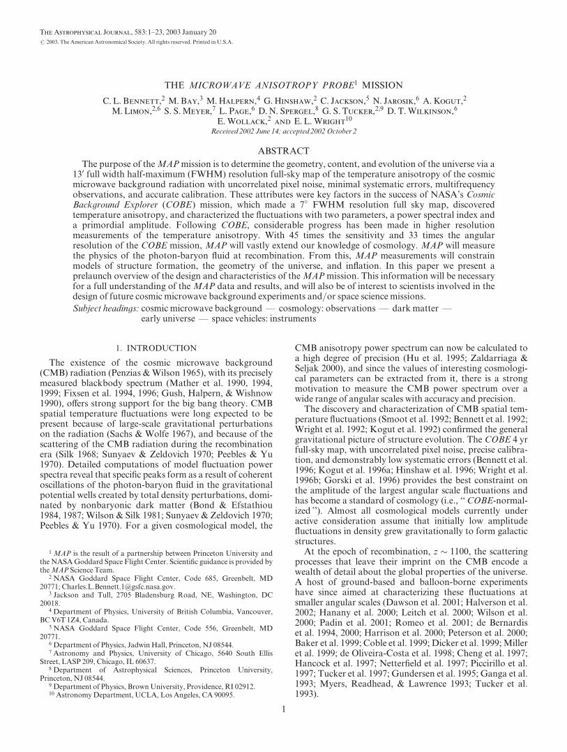
Figure 2 shows an overview of the MAP observatory. Adeployable Sun shield, with web blankets between solarpanels, keeps the spacecraft and instrument in shadow forall nominal science operations. Large passive radiators areconnected, via heat straps, directly to the high electronmobility transistor (HEMT) amplifiers at the core of theradiometers. A (94 cm diameter � 33 cm length � 0.318 cmthick) gamma-alumina cylindrical shell provides exception-ally low thermal conductance (0.59 and 1.4 W m�1 K�1 at80 and 300 K, respectively) between the warm spacecraftand the cold instrument components. The back-to-backoptical system can be seen as satisfying part of the require-ment for a symmetric differential design.

An L2 orbit was required to minimize thermal variationswhile simplifying the passive cooling design, and to isolatethe instrument from microwave emission from the Earth,Sun, andMoon. Figure 3 shows theMAP trajectory, includ-ing its orbit about L2.

Further systematic error suppression features of theMAPmission are discussed in the following subsections.

4.1. Thermal and Power Stability

There are three major objectives of the thermal design ofMAP. The first is to keep all elements of the observatorywithin nondestructive temperature ranges for all phases ofthe mission. The second objective is to passively cool theinstrument front-end microwave amplifiers and reduce themicrowave emissivity of the front-end components toimprove sensitivity. The third objective is to use only passivethermal control throughout the entire observatory to mini-mize all thermal variations during the nominal observingmode. While the first objective is common to all space mis-sions, the second objective is rare, and the third objective isentirely new and provides significant constraints to the over-all thermal design of the mission.

All thermal inputs toMAP are from the Sun, either fromdirect thermal heating or indirectly from the electrical dissi-pation of the solar energy that is converted in the solararrays. Since both thermal changes and electrical changesare potential sources of undesired systematic errors, meas-ures are taken to minimize both. The slow annual change inthe effective solar constant is easily accounted for. Varia-tions that occur synchronously with the spin period posethe greatest threat, since they most closely mimic a true skysignal.

To minimize thermal and electrical variations the solararrays maintain a constant angle relative to the Sun of22=5� 0=25 during CMB anisotropy observations at L2.The constant solar angle, combined with the battery, pro-vides for a stable power input to all electrical systems. Keysystems receive further voltage referencing and regulation.

To further minimize thermal and electrical systematiceffects, efforts are made to minimize variations in power dis-sipation. All thermal control is passive; there are no propor-tional heaters and no heaters that switch on and off (except forsurvival heaters that are only needed in cases of spacecraftemergencies, and the transmitter make-up heater, dis-cussed below). The electrical power dissipation changes ofthe various electronics boxes are negligible.

Passive thermal control required careful adjustment andtesting of the thermal blankets, radiant cooling surfaces,and ohmic heaters. A detailed thermal model was used toguide the development of a baseline design. Final adjust-ments were based on tests in a large thermal vacuum cham-ber, in which the spacecraft (without its solar panels) wassurrounded by nitrogen-cooled walls and the instrumentwas cooled by liquid helium walls.

Radio frequency interference (RFI) from the transmit-ter poses a potential systematic error threat to the experi-ment. Thus, there is a motivation to turn the transmitteron for only the least amount of time needed to downlinkthe daily data. However, the power dissipation differencebetween the transmitter on and off states poses a threat

passive thermalradiators

top deck

feed horns

Focal Plane Array (FPA) box

deployed solar arrayw/ web shielding

star trackers (2)

thrusters (8)

upper omni antenna

dual back-to-backGregorian optics

thermally isolatinginstrument cylinderReceiver Box (RXB)inside

truss structurewith microwavediffraction shielding

1.4 x 1.6 m primaryreflectors

secondaryreflectors

warm S/C andinstrument electronics

reactionwheels (3)

+Y

+X

-Z

Fig. 2.—View of theMAP observatory, shown with several of the major constituents called out. The observatory is 3.8 m tall, and the deployed solar arrayis 5.0 m in diameter. The observatorymass is 836 kg.


to thermal stability. To mitigate these thermal changes, a53 � make-up heater is placed on the transpondermounting plate to approximately match the 21 W ther-mal power dissipation difference between the on and offstates of the transmitter. There are two transponders(one is redundant), and they are both mounted to thesame thermal control plate. Both receivers are on at alltimes. The heater can be left on, except for the �40minute per day period that the transmitter must be used.Thus, there are two in-flight options for minimizing sys-tematic measurement errors due to the transmitter.Should in-flight RFI from the transmitter be judged agreater threat than residual thermal variations, then thetransmission time can be minimized and the make-upheater used. Alternately, should the residual thermal var-iations be the greater threat, the transmitter can be lefton continuously. The mission is designed such that eitheroption is expected to meet systematic error requirements.

There are scores of precision platinum resistance ther-mometers (PRTs) at various locations to provide aquantitative demonstration of thermal stability at the sub-millikelvin level. The information from these sensors isinvaluable for making a quantitative assessment of the levelof systematic errors from residual thermal variations andcould be used to make error corrections in the ground datareduction pipeline, if needed. The design is to make thesecorrections unnecessary and to use the sensor data only toprove that thermal variations are not significant.

4.2. Sky Scan Pattern

The sky scan strategy is critical to achieving minimal sys-tematic effects in CMB anisotropy experiments. The ideal

scan strategy would be to instantaneously scan the entiresky, and then rapidly repeat the scans so that sky regions aretraversed from all different angles. Practical constraints, ofcourse, limit the scan rate, the available instantaneous skyregion, and the angles through which each patch of sky istraversed by a beam. For a space mission, increasing thescan speed rapidly becomes expensive: it becomes more dif-ficult to reconstruct an accurate pointing solution, the tor-que requirements of on-board control components increase,and the data rates required to prevent beam smearingincrease. The region of sky available for scanning is limitedby the acceptable level of microwave pick-up from the Sun,Earth, andMoon.

It is possible to quantitatively assess the quality of a sky-scanning strategy by computer simulation. Systematicerrors are generated as part of an input to a computer simu-lation that converts time-ordered data to sky maps. Thesuppression factor of systematic error levels going fromthe raw time-ordered data into the sky map is a measure ofthe quality of the sky-scanning strategy. A poor scanningstrategy will result in a poor suppression factor. Our com-puter simulations show that the sky-scanning strategy usedby the COBEmission was very nearly ideal, as it maximallysuppressed systematic errors in the time-ordered data fromentering the map. A large fraction of the full sky wasscanned rapidly, consistent with avoiding a 60� full-anglecone in the solar direction. However, the Moon was often inand near the beam. This was useful for checks of amplitudeand pointing calibration, but much data had to be discardedwhen contamination by lunar emission was significant.COBE, in its low Earth orbit, also suffered from pick-up ofmicrowave emission from the Earth, also causing data to bediscarded.

1.5 x 106 km

Top View

Side View

1.5 x 108 km to Sun

Earth

Moon at swingby

L2

L2

Lunar orbit

Phasing loops

a0.010

0.005

0.000

-0.005

-0.0101.000 1.005 1.010

X (AU)

Y (A

U)

L2Earth

b

Fig. 3.—Views ofMAP ’s trajectory to an orbit about L2.MAP uses an L2 orbit to enable passive cooling and to minimize systematic measurement errors.(a) Perspective views (from the north ecliptic pole and from within the ecliptic plane) of a typical trajectory are shown in an Earth corotating coordinatesystem. An on-board reaction control (propulsion) system executes three highly elliptical ‘‘ phasing loop ’’ orbits about the Earth, which set up a gravity-assistlunar swing-by, and then a cruise to an orbit about the second Earth-Sun Lagrange point, L2. (b) Corotating gravitational potential. The break in contour linesrepresent a change of scale, where the gravitational potential near the Earth is much steeper than near L2. Tick marks indicate the ‘‘ down-hill ’’ side of eachcontour. The L2 orbit provides a quasi-stable orbit in a saddle-shaped gravitational potential. This is a ‘‘ Lissajous ’’ rather than ‘‘ halo ’’ orbit, since theobservatory is at a different position with a different velocity vector after each 6month loop.


In its nominal L2 orbit the MAP observatory executes acompound spin (0.464 rpm) and precession (1 hr�1), asshown in Figure 4. TheMAP sky scan strategy is a compro-mise. While the MAP scan pattern is almost as good asCOBE’s with regard to an error-suppression factor, it is farbetter than COBE’s for rejecting microwave signals fromthe Sun, Earth, and Moon. The MAP sky scan patternresults in full sky coverage with some variation in the num-ber of observations per pixel, as shown in Figure 4.

To make a sky map from differential observations, it isalso essential for the pixel-pair differential temperatures tobe well interconnected between as many pixel pairs as possi-ble. The degree and rate of convergence of the sky map solu-tion depends upon it. The MAP sky scan pattern can beseen, in computer simulation, to enable the creation of mapsthat converge in a rapid and well-behaved manner.

4.3. MultifrequencyMeasurements

Galactic foreground signals are distinguishable fromCMB anisotropy by their differing spectral and spatial dis-tributions. Figure 5 shows the estimated spectra of thegalactic foreground signals relative to the cosmological sig-nal. Four physical mechanisms that contribute to the Galac-tic emission are synchrotron radiation, free-free radiation,thermal radiation from dust, and radiation from chargedspinning dust grains (Erickson 1957; Finkbeiner et al. 2002;Draine & Lazarian 1998a, 1998b, 1999). MAP is designedwith five frequency bands, seen in Figure 5, for the purposeof separating the CMB anisotropy from the foregroundemission.

Microwave and other measurements show that at highGalactic latitudes ( bj j > 15�) CMB anisotropy dominatesthe Galactic signals in the frequency range �30–150 GHz

(Tegmark et al. 2000; Tegmark & Efstathiou 1996). How-ever, the Galactic foreground will need to be measured andremoved from some of the MAP data. There are three con-ceptual approaches that can be used, individually or in com-bination, to evaluate and remove the Galactic foreground.

The first approach is to use existing Galactic maps atlower (radio) and higher (far-infrared) frequencies as fore-ground emission templates. These emission patterns can bescaled to the MAP frequencies and subtracted. Uncertain-ties in the external data and scaling errors due to position-dependent spectral index variations are the major weak-nesses of this technique. There is no good microwave free-free emission template because there is no frequency whereit clearly dominates the microwave emission. High-resolution, large-scale maps of H� emission (L. M. Haffneret al., in preparation; Gaustad et al. 2001; see also theVirginia Tech Spectral-Line Survey11) can serve as a tem-plate for the free-free emission, except in regions of high H�optical depth. The spatial distribution of synchrotron radia-tion has been mapped over the full sky with moderate sensi-tivity at 408 MHz (Haslam et al. 1981). Low-frequency(<10 GHz) spectral studies of the synchrotron emissionindicate that the intensities are reasonably described by apower law with frequency S / ��, where Sð�Þ is the fluxdensity, or T / ��2 � ��, where Tð�Þ is the antenna tem-perature and � � �2:7, although substantial variationsfrom this mean occur across the sky (Reich & Reich 1988).There is also evidence, based on the local cosmic-ray elec-tronic energy spectrum, that the local synchrotron spectrumshould steepen with frequency to � � �3:1 at microwave

11 The Virginia Tech Spectral-Line Survey is available at: http://www.phys.vt.edu/~halpha.

Fig. 4.—(a) Full sky map projection in ecliptic coordinates, showing the number of independent data samples taken per year by sky position. Full skycoverage results from the combined motions of the spin, precession, and orbit about the Sun. The spin axis precesses along the red circle in 1 hr. When the spinaxis is at the position of the blue cross, a feed pair traces the green circle on the sky in the 129 s spin period. The white circles indicate the results of theprecession. Full sky coverage is achieved in 6 months asMAP orbits around the Sun (with the Earth). (b) The number of observations per pixel as a function ofecliptic latitude is shown for each full year of observations. The number of observations per pixel will vary by frequency band because of differing samplingrates, differing beam solid angles, and data flagging. The plot is illustrative; theMAP datamust be used for exact sky-sampling values.


Fig. 5.—CMB vs. foreground anisotropy. The frequency bands were chosen so thatMAP observes the CMB anisotropy in a spectral region where the emis-sion is most dominant over the competing Galactic and extragalactic foreground emission. (a) Spectra of CMB anisotropy (for a typical �CDM model) andestimates of Galactic emission. A component traced by the Haslam spatial template (red ) must be steep (� < �3:0) because of its lack of correlation with theCOBEmaps. (Note, however, that any template map of synchrotron emission will be frequency-dependent, and hence the lack of correlation between Haslamandmicrowavemaps is likely due to spatially variable spectral indices.) The free-free component ( pink) estimate is fromH� data (L.M. Haffner et al., in prep-aration; Gaustad et al. 2001), converted assuming 2 lK R�1 at 53 GHz and a �2.15 spectral index. A component traced by 100 lm dust emission (blue) has aspectral index of � � �2:3 (Kogut et al. 1996b). This is likely to include the flat spectrum synchrotron emission that is relatively under-represented by the 408 MHz Haslam template, but may be most of the synchrotron emission at microwave/millimeter wavelengths. Spinning dust emissioncomponents should be picked up in the H� ( pink) and 100 lm (blue) estimates. The three component estimates above are partially redundant, so they areadded in quadrature to arrive at the estimate for the overall combined foreground spectra (dashed curves). The thermal dust emission model (green) of Fink-beiner et al. (1999) is a fit to COBE data. The total Galactic emission estimate is shown for cuts of the brightest microwave sky regions, leaving 60% and 80%of sky. (b) The spatial spectra are shown, in thermodynamic temperature, relative to a typical �CDM CMB model. We have masked 20% of the brightestGalactic sky. The extragalactic source contribution of Toffolatti et al. (1998) is used with the assumption that sources down to 0.1 Jy have been removed. (c)The contour plot shows the ratio of CMB to foreground anisotropy power as a function of frequency and multipole moment. As can be seen, theMAP bandswere chosen to be in the only region where the CMB anisotropy power is >10 times to >100 times that of the competing foregrounds. TheMAP bands extendto an lmax such that the beamwindow function is 10%.

frequencies (Bennett et al. 1992). However, this steepeningeffect competes against an effect that flattens the overallobserved spectrum. The steep spectral index synchrotroncomponents seen at low radio frequencies become weak rel-ative to any existing flat spectral index components as onescales to the higher microwave frequencies. The synchro-tron signal is complex because individual source compo-nents can have a range of spectral indices, causing asynchrotron template map of the sky to be highly frequencydependent. The dust distribution has been mapped over thefull sky in several infrared bands, most notably by theCOBE and IRAS missions. A full-sky template is providedby Schlegel, Finkbeiner, & Davis (1998) and is extrapolatedin frequency by Finkbeiner, Davis, & Schlegel (1999).

The second approach is to form linear combinations ofthe multifrequency MAP sky maps such that the Galacticsignals with specified spectra are canceled, leaving only amap of the CMB. The linear combinations of multifre-quency data make no assumptions about the foregroundsignal strength, but require knowledge of the spectra of theforegrounds. The dependence on constant spectral indiceswith frequency in this technique is less problematic than inthe template technique given above, since the frequencyrange is smaller. The other advantage of this method is thatit relies only onMAP data, so the systematic errors of otherexperiments do not enter. The major drawback to this tech-nique is that it adds significant extra noise to the resultingreduced Galactic emission CMBmap.

The third approach is to determine the spatial and/orspectral properties of each of the Galactic emission mecha-nisms by performing a fit to either the MAP data alone, orin combination with external data sets. Tegmark et al.(2000) is an example of combining spectral and spatial fit-ting. Various constraints can be used in such fits, as deemedappropriate. A drawback of this approach is the low signal-to-noise ratio of each of the Galactic foreground compo-nents at high Galactic latitude. This approach also addsnoise to the resulting reduced Galactic emission CMBmap.

All three of these techniques were employed with somedegree of success with the COBE data (Bennett et al. 1992).In the end, these techniques served to demonstrate that,independent of technique, a cut of the strongest regions offoreground emission was all that was needed for most cos-mological analyses.

In addition to the Galactic foregrounds, extragalacticpoint sources will contaminate the MAP anisotropy data.Estimates of the level of point-source contaminationexpected at the MAP frequencies have been made based onextrapolations from measured counts at higher and lowerfrequencies (Park, Park, & Ratra 2002; Sokasian, Gawiser,& Smoot 2001; Refregier, Spergel, &Herbig 2000; Toffolattiet al. 1998). Direct 15 GHz source count measurements byTaylor et al. (2001) indicate that these extrapolated sourcecounts underestimate the true counts by a factor of 2. This isbecause, as in the case of Galactic emission discussed above,flatter spectrum synchrotron components increasinglydominate over steeper spectrum components with increas-ing frequency. Microwave/millimeter wave observationspreferentially sample flat spectrum sources. Techniques thatremove Galactic signal contamination, such as the onesdescribed above, will also generally reduce extragalacticcontamination. For both Galactic and extragalactic con-tamination, the most affectedMAP pixels should be maskedand not used for cosmological purposes. After applying a

point-source and Galactic signal minimization techniqueand masking the most contaminated pixels, the residualcontribution must be accounted for as a systematic error.

Hot gas in clusters of galaxies will also contaminate themaps by shifting the spectrum of the primary anisotropy tocreate a Sunyaev-Zeldovich decrement in the MAP fre-quency bands. This is expected to be a small effect forMAP,and masking a modest number of pixels at selected knowncluster positions should be adequate.

Figures 5 illustrates how the MAP frequency bands werechosen to maximize the ratio of CMB-to-foreground aniso-tropy power. After applying data cuts for the most contami-nated regions of sky, the methods discussed above areexpected to substantially reduce the residual contamination.

5. INSTRUMENT DESIGN

5.1. Overview

The instrument consists of back-to-back Gregorianoptics that feed sky signals from two directions into 10 four-channel polarization-sensitive receivers (‘‘ differencingassemblies ’’). The HEMT amplifier-based receivers coverfive frequency bands centered from 23 to 93 GHz. Each pairof channels is a rapidly switched differential radiometerdesigned to cancel common-mode systematic errors. Thesignals are square-law detected, voltage-to-frequency digi-tized, and then downlinked.

5.2. Optical Design

The details of the MAP optical design, including beampatterns and sidelobe levels, are discussed by Page et al.(2003). We provide an overview here.

Two sky signals, from directions separated in azimuth by�180� and in total angle by �141�, are reflected via twonearly identical back-to-back primary reflectors towardstwo nearly identical secondary reflectors and into 20 feedhorns, 10 in each optical path. The off-axis Gregorian designallows for a sufficient focal plane area, a compact configura-tion that fits in the Delta-rocket fairing envelope, two oppo-site-facing focal planes in close proximity to one another,and an unobstructed beamwith low sidelobes. The principalfocus of each optical path is between its primary and itssecondary.

The reflector surfaces are ‘‘ shaped ’’ (i.e., designed withdeliberate departures from conic sections) to optimize per-formance. YRS Associates of Los Angeles, CA, carried outmany of the relevant optical optimization calculations.Each primary is a (shaped) elliptical section of a paraboloidwith a 1.4 m semiminor axis and a 1.6 m semimajor axis.When viewed along the optical axis, the primary has a circu-lar cross section with a diameter of 1.4 m. The secondaryreflectors are 0:9 m� 1:0 m. The reflectors are constructedof a thin carbon fiber shell over a Korex core, and are fixed-mounted onto a carbon-composite (XN-70 and M46-J)truss structure. The reflectors and their supporting trussstructure were manufactured by Programmed CompositesIncorporated. Use of the composite materials minimizesboth mass and on-orbit cool-down shrinkage. The reflectorsare fixed-mounted so as to be in focus when cool, so ambientpreflight measurements are slightly out of focus. The reflec-tors have approximately 2.5 lm of vapor-deposited alumi-num and 2.2 lm of vapor-deposited silicon oxide (SiOx).The silicon oxide over the aluminum produces the required

MAP MISSION 9

surface thermal properties (a solar absorptivity to thermalemissivity ratio of �0.8 with a thermal emissivity of �0.5)while negligibly affecting the microwave signals. The micro-wave emissivity of coupon samples of the reflectors weremeasured in the lab to be that of bulk aluminum. The coat-ings were applied by Surface Optics Incorporated.

The layout and polarization directions of the 10 feeds,covering five frequency bands, are shown in Figure 6. Thefeed designs are driven by performance requirements (side-lobe response, beam symmetry, and emissivity), and byengineering considerations (thermal stress, packaging, andfabrication considerations), and by the need to assure closeproximity of each feed tail to its differential partner.

The feeds are designed to illuminate the primary equiva-lently in all bands; thus, the feed apertures approximatelyscale with wavelength. The smallest, highest frequency feedsare placed near the center of the focal plane, where beampattern aberrations are smallest. The HE11 hybrid modedominates the corrugated feed response, giving minimalsidelobes with high beam symmetry and low loss. The low-est frequency feeds are profiled to minimize their length,while the highest frequency feeds are extended beyond theirnominal length so that all feeds are roughly of the samelength. The feeds were specified and machined by PrincetonUniversity and designed by YRS Associates. They are dis-cussed in greater detail by Barnes et al. (2002).

5.3. Radiometer Design

The details of the radiometer design, including noise and1/f properties, are discussed by Jarosik et al. (2003). Weprovide an overview here.

MAP’s ‘‘ microwave system ’’ consists of 10 four-channeldifferencing assemblies, each of which receives two orthogo-nally polarized signals from a pair of feeds. Each differenc-ing assembly has both warm and cold amplifiers. The coldportion of each differencing assembly is mounted and pas-sively cooled in the focal plane assembly (FPA) box; thewarm portion is mounted in the receiver box (RXB).

As seen in Figure 7, the signal from each feed passesthrough a low-loss orthomode transducer (OMT), whichseparates the signal into two orthogonal polarizations. TheA-side signal is differenced against the orthogonally polar-ized signal from the opposite feed, B0. This differencing isaccomplished by first combining A and B0 in a hybrid Tee,amplifying the two combined outputs in two cold HEMTamplifiers, and sending the outputs to the RXB via wave-guide. In the RXB the two signals are amplified in two warmHEMT amplifiers. Then one signal path is phase switched(0� or 180� relative to the other) with a 2.5 kHz square-wavemodulation. The two signals are combined back into A andB0 by another hybrid Tee, filtered, square-law detected,amplified by two line drivers, and sent to the analog elec-tronics unit (AEU) for synchronous demodulation and digi-tization. The other pair of signals, A0 and B, are differencedin the same manner. In MAP jargon, each of these pairs ofsignals comes from a ‘‘ radiometer ’’ and both pairs togetherform a ‘‘ differencing assembly.’’ In all, there are 20 statisti-cally independent signal ‘‘ channels.’’

The splitting, phase switching, and subsequent combiningof the signals enhances the instrument’s performance in twoways: (1) since both signals to be differenced are amplifiedby both amplifier chains, gain fluctuations in either ampli-fier chain act identically on both signals, so common mode

cm

cm

cm

Side A Focal Plane Side B Focal Plane

10 cm4.4 cm/deg on sky

KaK

V2V1

Q1

W2 W3

W1 W4

Q2

KaK

V1V2

Q2

W3 W2

W4 W1

Q1

Fig. 6.—View of the focal plane feed layout in the focal plane assembly (FPA) as seen from the secondaries. The A side is the +y direction and the B side isthe�y direction. The cross-hatch indicates the direction of the E-plane polarization for the axial OMT port. Each radiometer is named after the position of itsfeed pair, and the OMT ports to which it attaches. (We sometimes refer to feeds K and Ka as K1 and Ka1 despite the lack of a K2 and Ka2.) For example, forthe radiometer V21, the last digit 1 corresponds to the axial OMT port, while a last digit of 2 would indicate the radial OMT port. Radiometer V21 differencesthe polarizations shown by the hatching in this figure. Radiometer V22 differences the opposite polarizations. With this convention, the meanings of all of theradiometer names can be immediately found from the above diagram.

10 BENNETT ET AL.

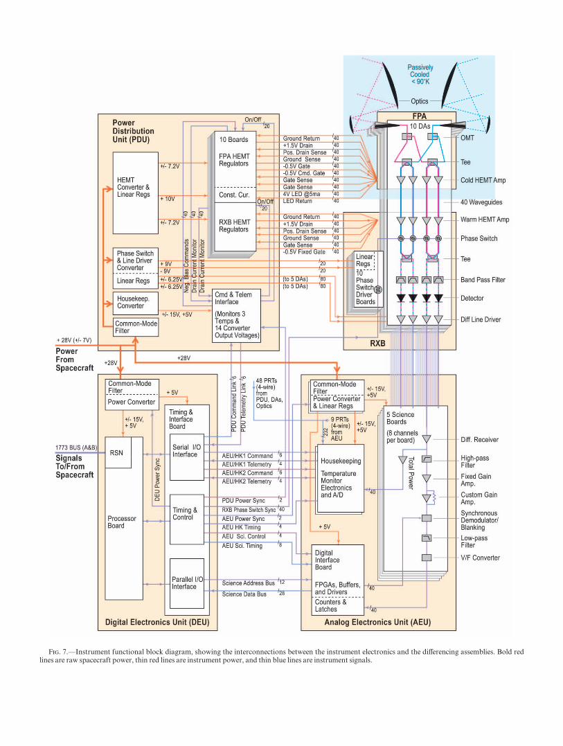
Fig. 7.—Instrument functional block diagram, showing the interconnections between the instrument electronics and the differencing assemblies. Bold redlines are raw spacecraft power, thin red lines are instrument power, and thin blue lines are instrument signals.

gain fluctuations cancel; and (2) the phase switches introducea 180� relative phase change between two signal paths,thereby interchanging which signal is fed into each square-law detector. Thus, low-frequency (1/f ) noise from the detec-tor diodes is common mode and also cancels, further reducingsusceptibility to systematic effects.

The first-stage amplification operates at a stable low tem-perature to obtain the required sensitivity. HEMT amplifiernoise decreases smoothly and only gradually with cooling;there are no sharp break points. HEMT amplifiers exhibitlarger intrinsic gain fluctuations when operated cold thanwhen operated warm, so as many gain stages as possibleoperate warm, consistent with achieving the optimal systemnoise temperature.

The gate voltage of the first stage of the cold HEMTamplifiers is commandable in flight to allow amplifier per-formance to be optimized after the FPA has cooled to asteady-state temperature or as the device ages. Each pair ofphase-matched chains (both the FPA and RXB portions)can be individually powered off in flight to prevent anyfailure modes (parasitic oscillations, excessive power dissi-pation, etc.) from interfering with the operation of otherdifferencing chains.

The frequency bands (Jarosik et al. 2003; Page et al. 2003)were chosen to lie within commercial standards to allow theuse of off-the-shelf components. The HEMT amplifiers(Pospieszalski 1992, 1997; Pospieszalski et al. 1994, 2000)were custom-built forMAP by the National Radio Astron-omy Observatory, based on custom designs by MarianPospieszalski. The HEMT devices were manufactured byLoi Nguyen at Hughes Research Laboratories. The highestfrequency band used unpassivated devices, and the lowerfour frequency bands used passivated devices. The phaseswitches and bandpass filters were manufactured by PacificMillimeter, the Tees and diode detectors by Millitech, theOMTs by Gamma-f, the thermal-break waveguide by Cus-tom Microwave and Aerowave. Absorber materials, whichare used to damp potential high-Q standing waves in thebox cavities of the FPA and RXB, are from Emerson &Cummings. The differencing assemblies were assembled,tested, and characterized at Princeton University, and theFPA and RXB were built up, aligned, tested, and character-ized with their flight electronics at Goddard.

While noise properties were measured on the ground, thedefinitive noise values must be derived in flight, since theyare influenced by the specific temperature distributionwithin each radiometer.

The output of a square-law detector for an ideal differen-tial radiometer is a voltage,V, per detector responsivity, s,

V

s¼ A2 þ B2

2þ n1

� �g21ðtÞ

þ A2 þ B2

2þ n2

� �g22ðtÞ �

A2 � B2

2g1ðtÞg2ðtÞ ;

where g and n are the total gain and noise of each arm of aradiometer and A and B are the input voltages at the frontend of the radiometers. The first two terms are the totalpower signals. The � on the third term alternates with the2.5 kHz phase-switch rate, with the two arms of the radio-meter always having opposite signs from one another. Thedifference between paired detector outputs for an ideal sys-tem, V=s ¼ ðA2 � B2Þg1ðtÞg2ðtÞ ¼ ðTA � TBÞg1ðtÞg2ðtÞ, is

used to make the sky maps. See Jarosik et al. (2003) for adiscussion of the effects of deviations from an ideal system.

5.4. Instrument Electronics Design

There are three instrument electronic components (seeFig. 7). The power distribution unit (PDU) provides theinstrument with its required regulated and filtered powersignals. The analog electronics unit (AEU) demodulatesand filters the instrument detector outputs and convertsthem into digital signals. The digital electronics unit (DEU),built into the same aluminum housing as the AEU, holdsthe instrument computer and provides the digital interfacebetween the spacecraft and the PDU and AEU. The instru-ment electronics were built at Goddard.

The five science boards in the analog electronics unit(AEU) take in the 40 postdetection signals from the RXB’sdifferencing assemblies through differential receivers. The40 total power signals are split off and sent to the AEUhousekeeping card for eventual telemetry to the ground.The total power signals are not used in making the sky mapsbecause of their higher susceptibility to potential systematiceffects, but they are useful signals for tracing the operationof the differencing assemblies and the experiment as awhole. After the total power signal is split off, the remainingsignal is sent through a high-pass filter, a fixed gain ampli-fier, and then through another fixed-gain amplifier whosegain is set on the ground using precision resistors to accom-modate the particular differencing assembly signal level.The signal is then demodulated synchronously at the 2.5kHz phase-switch rate. A blanking period of 6 ls (from 1 lsbefore through 5 ls after the switch event) is supplied toavoid systematic errors due to switching transients. The�40 Hz bandwidth demodulated signal is then sent througha two-pole Bessel low-pass filter with its 3 dB point at 100Hz. Finally, the signal is sent through a voltage-to-fre-quency (V/F) converter, whose output is latched for read-out by the processor in the digital electronics unit (DEU),before being losslessly compressed and telemetered to theground. The AEU has a digital interface board and twopower converter boards, which supply the requisite �15 V,�12 V, and +5 V to the other AEU boards.

The noise in each of the 40 AEU signal channels is limitedto under 150 nV Hz�0.5 from 2.5 to 100 kHz to ensure thatthe AEU contributes less than 1% of the total radiometernoise. The AEU channel bandwidth is 100 kHz. The gaininstability is less than 5 ppm for synchronous variationswith the observatory spin. This requires that the compo-nents be thermally stable to less than 10 mK at the observa-tory spin rate. Random gain instabilities are limited to lessthan 100 ppm from 8 mHz (the spin frequency) to 50 Hz.The DC-coupled amplifier has random offset variations ofless than 1 mV rms from 8 mHz to 50 Hz to limit its contri-bution to the post-demodulation noise.

The AEU also contains two boards for handling voltageand high-precision temperature sensing of the instrument.These monitors go well beyond the usual health and safetyfunctions; they exist primarily to confirm voltage and ther-mal stability of the critical items in the instrument. Shouldvariations be seen, these monitor signals can be used as trac-ers and diagnostics to characterize the effects on the sciencesignals.

The DEU receives power from the spacecraft bus (fedthrough the PDU), applies a common-mode filter, and uses


a DC-DC power converter to generate +5 V and �15 V forinternal use on its timing and interface board and on its pro-cessor board. The power converter is on one card, while theremote services node (RSN; see x 6.1) and timing boards areon opposite sides of a double-sided card.

The DEU provides a 1 MHz (�0.005%, 50% duty cycle)clock, derived from a 24 MHz crystal oscillator, to the V/Fconverter in the AEU. The DEU also supplies a 100 kHzclock to the power converters in the PDU and the AEU, a2.5 kHz (50% duty cycle) clock to the RXB and AEU forphase switching, and a 5 kHz pulse to the AEU for blankingthe science signal for 6 ls during the 2.5 kHz switch transi-tions. The DEU also provides a 25.6 ms (64 cycles at 2.5kHz = 39.0625 Hz) 1 ls wide negative logic clock to theAEU for latching the 14 bit science data samples. All 40channels are integrated in the AEU and sent to the DEUevery 25.6 ms, as shown in Figure 8. The RF bias (totalpower) signals from the 40 AEU channels, and 57 platinumresistance thermometer (PRT) temperature signals arepassed from the AEU to the DEU every 23.04 s. All of theseDEU clock signals are synchronous with the 24 MHz mas-ter clock. The DEU also sends voltage, current, and internaltemperature data from the PDU, AEU, and DEU.

The 69R000 processor in the DEU communicates withthe main computer (see x 6.1) over a 1773 optical fiber bus.The DEU uses 12K (16 bit words) memory for generic RSNinstruction code, 24K for DEU-specific code, and 10K fordata storage.

The AEU and DEU are packaged together in an alumi-num box enclosure with shielding between the AEU andDEU sections. The AEU/DEU and the PDU dissipate90%–95% of their power from their top radiators. They arequalified over a�10� to +50�C temperature range, but nor-mally operate over a 0�–40�C range. The temperature varia-tions of the boxes are designed to be limited to less than 10

mK peak-to-peak at the spin period. The 100 mil effectivebox wall thicknesses allow the electronics to survive thespace radiation environment (see x 6.6.2).

The PDU receives 21–35 V from the spacecraft, withspin-synchronous variations of less than 0.5 V peak-to-peak, and provides all instrument power. Every HEMT gateand drain is regulated with a remote-sense feedback circuit.The PDU clamps the voltage between the gate and drain tobe less than 2.1 V (at 10 lA) to prevent damage to the sensi-tive HEMT devices. The drain voltages are commandable ineight steps (�70 mV resolution) from 1.0 to 1.5 V, and thegates are commandable in 16 steps (�35 mV resolution)from �0.5 to 0 V. Voltage drifts are510 mV for the drain,and55 mV for the gates over the 0�–40�C operating range.

The broadband noise requirements on the HEMT gateand drain supplies are: less than 23f�0.45 lV Hz�0.5 for 0.3mHz–1 Hz (= 885 lV Hz�0.5 at 0.3 mHz); less than 23 lVHz�0.5 for 1–50 Hz; and less than 100 nV Hz�0.5 for 2.5 kHzand its harmonics to 50 kHz. These frequency ranges corre-spond to the precession frequency (�0.3 mHz), the spin fre-quency (�7.57 mHz), and the phase-switch frequency (�2.5kHz), respectively. Spin-synchronous rms variations are lessthan 400 nV.

The PDU supplies 4 V at 5 mA (<5 nA rms variation atthe spin period) to two series LEDs on each cold HEMTamplifier. The LED light helps to stabilize the gain of theHEMT devices.

The PDU supplies �9 V (<50 mV ripple, <20 mV com-mon mode noise) to the phase-switch driver cards, whichare mounted in the RXB, near the differencing assemblies.The PDU also supplies �6.25 V to the line drivers in theRXB.

The PDU allows for on/off commands to remove powerfrom any one or more of the 20 radiometers (phase-matchedhalves of the differencing assemblies). Should several radio-meters be turned off, such that the lack of power dissipationdrives the PDU temperature out of its operational tem-perature range, a supplemental make-up heater can becommanded on to warm the PDU.

5.5. Instrument Calibration

The instrument is calibrated in flight using observationsof the CMB dipole and of Jupiter, as discussed in x 7.1.

Despite the in-flight amplitude calibration (telemetry dig-ital units per unit antenna temperature), it was necessary toprovide provisional calibration on the ground to assess andcharacterize various aspects of the instrument to assure thatall requirements would be met. For example, cryogenicmicrowave calibration targets (‘‘ x-cals ’’) were designed andbuilt to provide a known temperature for each feed horninput for most ground tests. The x-cals, attached directly toeach of the 20 feed apertures, were individually tempera-ture-controlled to a specified temperature in the range of15–300 K, and provided for temperature readout.

Observations of Jupiter and other celestial sources pro-vide an in-flight pointing offset check relative to the star-tracker pointing. The pointing directions of the feeds weremeasured on the ground using standard optical alignmenttechniques. Jupiter also serves as the source for beam pat-tern measurements in flight. Beam patterns were measuredin an indoor compact antenna range at the Goddard SpaceFlight Center, and the far sidelobes were measured betweenrooftops at PrincetonUniversity.

V Band (61 GHz)

Q Band (41 GHz)

Ka Band (33 GHz)

K Band (23 GHz)

16

1

1

8

1

8

1

4

1

4

30 samples/channel2 x 25.6 = 51.2 msec/sample W Band (93 GHz)

20 samples/channel3 x 25.6 = 76.8 msec/sample

15 samples/channel4 x 25.6 = 102.4 msec/sample

12 samples/channel5 x 25.6 = 128 msec/sample

12 samples/channel5 x 25.6 = 128 msec/sample

1.536 sec

W4

W3

W2

W1

V2

V1

Q2

Q1

Ka1

K1

Fig. 8.—All 40 channels from the 10 differencing assemblies, sampled inmultiples of an underlying 25.6 ms period. The number of 25.6 ms periodsthat make up each sample is chosen with regard to the beamwidth of thatchannel to avoid smearing a source on the sky. Every 1.536 s the samplesare collected and put into packets for later data downlink.


6. OBSERVATORY DESIGN

This section provides an overview of theMAP spacecraftsystems. The physical layout of the observatory is shown inFigure 9, and the functional block diagram is shown inFigure 10.

6.1. Command and Data Handling

MAP implements a distributed architecture with a centralMongoose computer, which communicates via a 1773(Spectran 171.2 lm 1300 nm polyamide) fiber optic bus toremote services nodes (RSNs) located in the electronicsboxes (see Fig. 10). Each RSN provides a standardizedinterface to analog and digital electronics and uses commonflight software. The RSN circuitry occupies half of one sideof a printed circuit card; the remainder of the card space isused for application-specific circuitry. The fiber optics areinterconnected using two (redundant) star couplers. Eachis a pigtail coupler with a 16� 16 configuration in a8:9� 20� 4:4 cm aluminum housing.

Attitude control electronics (ACE) and command anddata handling (C&DH) functions are housed in the MidexACE and C&DH (MAC) box, which contains nine boards:(1) a Mongoose V R3000 32 bit rad-hard RISC processorboard including 4 MB of EEPROM memory and 320 MBof DRAM memory (of which 224 MB is for the solid statedata ‘‘ recorder,’’ 32 MB is for code, and 64 MB is for checkbytes), with 4 Mbps serial outputs to the transponder inter-face boards and redundant 1773 interfaces; (2, 3) two lowvoltage power converter (LVPC) boards (see x 6.4); (4, 5)two up- and downlink transponder boards, which are bothalways active (see x 6.3); (6) a housekeeping board, whichmonitors six deployment potentiometers (see x 6.5), ninestatus indicators, 46 temperature channels, and two vol-tages, in addition to one spare word, for a total of 64 inputsignals; (7) an ACE RSN and sensor electronics I/O board,which reads the digital and coarse Sun sensors, and readsand commands the reaction wheels (see x 6.2); (8) an ACEsensor I/O board that queries and/or reads informationfrom the inertial reference unit (gyro), digital and analogSun sensors, reaction wheels, separation switches (see x 6.2),and sends a timing pulse to the star trackers and monitorsthermistors and solar array potentiometers; and (9) a pro-pulsion engine valve drive (EVD) electronics board thatcontrols the eight thrusters (see x 6.2).

Selected redundancy is provided by a ‘‘ little MAC,’’ orLMAC box. The LMAC box houses a total of six boards.Four boards hold the redundant attitude control electronics(an LVPC board, a EVD electronics board, a sensor I/Oboard, and an RSN board). The two remaining boards are aredundant Mongoose processor board and a LVPC boardwith power-switching circuitry that controls the redundancybetween the MAC and the LMAC functions. Only oneMongoose processor (MAC or LMAC) is on and in controlat any one time. Shortly after launch the LMAC ACE takesprimary control, with the MAC ACE powered on as a‘‘ hot ’’ back-up. The active Mongoose processor boardsends an ‘‘ I’m OK ’’ signal to the LMAC ACE. If theLMACACE fails to get the ‘‘ I’m OK ’’ signal, then it placesthe observatory into safe-hold. That is, the ACE RSN actsas an attitude control safe-hold processor. If the housekeep-ing RSN fails, the LMAC ACE is powered on by groundcommand. Only a single uplink path can be active, selectedby ground command.

6.1.1. Data Sampling and Rates

The MAC Mongoose processor gathers the observatoryscience and engineering data and arranges them in packetsfor downlink. The instrument’s compressed science datacomprise 53% of the total telemetry volume.

As shown in Figure 8, during a 1.536 s period the instru-ment collects 30 samples in each of 16 W-band (93 GHz)channels, 20 samples in each of eight V-band (61 GHz)channels, 15 samples in each of eight Q-band (41 GHz)channels, and 12 samples in each of four Ka-band (33 GHz)and four K-band (23 GHz) channels. In this way, the bandswith smaller beams are sampled more often. With 856 sam-ples all together at 16 bits per sample in 1.536 s, there is atotal instrument science data rate of 8917 bits s�1. Theinstrument science data are put into two packets, with all ofthe W-band data in one packet and all other data in a sec-ond packet. The second packet is assigned some additionalfiller to make the two packet lengths identical. Each packetalso has 125 bits s�1 of ‘‘ packaging ’’ overhead. Theadjusted total raw instrument data rate is 9042 bits s�1.These data flow from the DEU to theMAC.

The Mongoose V processor losslessly compresses thisdata on-the-fly by a factor of �2.5 using the Yeh-Rice algo-rithm, and then records 3617 bits s�1 of science data. Anadditional 500 bits s�1 of instrument housekeeping data and2750 bits s�1 of spacecraft data are recorded, for a total of6867 bits s�1. The �0.6 Gbits of data per day are down-linked daily. Of the overall downlink rate of 666,666 bitss�1, 32,000 bits s�1 are dedicated to real-time telemetry, and56,3167 bits s�1 are allocated to the playback of the storeddata, which takes 17.6 minutes. The bit rate is commandableand may be adjusted in flight depending on the link marginsactually achieved.

6.1.2. Timing Control

The Mongoose board in the MAC/LMAC maintainstime with a 32 bit second counter and a 22 bit microsecondcounter. There is also a watchdog timer and a 16 bit externaltimer. The clock is available to components on the bus witha relative accuracy of 1 ms. Data are time-tagged so that arelative accuracy of 1.7 ms can be achieved between the startracker(s), gyro, and the instrument. The observatory timeis correlated to ground time to within 1 s.

6.2. Attitude and Reaction Control

The attitude control system (ACS) takes over control ofthe orientation of the observatory after its release from theDelta vehicle’s third stage. From the postseparation 3 � ini-tial conditions (�2� s�1 x- and y-axis tip-off rates, and �2rpm z-axis de-spin rate), MAP is designed to achieve apower-positive attitude (solar array normal vector within25� of the Sun direction) within 37 minutes using only itswheels for up to 2 � tip-off rates.

The attitude control and reaction control (propulsion)systems bring MAP through the Earth-Sun phasing loops(see Fig. 3) such that the thrust is within �5� of the desiredvelocity vector with 1� maneuver accuracy. After the lunarswing-by, MAP cruises, with only slight trajectory-correc-tion midcourse maneuvers, into an orbit about L2. Oncethere, the ACS provides a combined spin and precessionsuch that the observatory spin (z) axis remains at22=5� 0=25 from the Sun vector for all science observations.

14 BENNETT ET AL.

Fig. 9.—Physical layout of theMAP observatory, shown from various perspectives

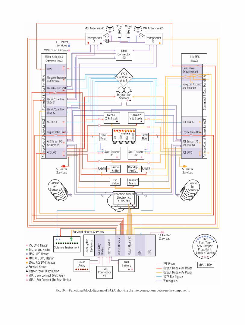
Fig. 10.—Functional block diagram ofMAP, showing the interconnections between the components

This is referred to as the ‘‘ observing mode.’’ For all maneu-vers that interrupt the observing mode (after the midcoursecorrection on the way to L2, and for station-keepingmaneuvers at L2), the spin (z) axis must always remain at19� � 5� relative to the Sun vector to prevent significantthermal changes. The spin rate must be an order of magni-tude higher than the precession rate, and the instrumentboresight scan rate must be 2=59 s�1 to 2=66 s�1. The 2=784s�1 (0.464 rpm) spin and the 0=100 s�1 (0.017 rpm, 1 revhr�1) precession rates are in opposite directions and are con-trolled to within 6%. The ACS must also manage momen-tum and provide an autonomous safe-hold. Momentummanagement occurs throughout the mission, with eachmomentum unload leavingd0.3 Nms per axis.

The instrument pointing knowledge requirement of 1<3 (1�) is sufficient for the aspect reconstruction needed to placethe instrument observations on the sky. Of this, 0<9 (a root-sum-square for three axes) is allocated to the attitude con-trol system.

The radius of the Lissajous orbit about L2 (see Fig. 3)must bee0=5 (between the Sun-Earth vector and the Earth-MAP vector) to avoid eclipses, and less than 10=5 to main-tain the antenna angles necessary for a sufficient communi-cation link margin.

The attitude and reaction control systems include attitudecontrol electronics (ACE boards, in both the MAC andLMAC boxes), three reaction wheels, two digital Sun sen-sors, six prime plus six redundant coarse Sun sensors, onegyro (mechanical dynamically tuned, consisting of two two-axis rate assemblies [TARAs]), and two star trackers (oneprime and one redundant). The propulsion system consistsof two engine valve drive cards (one in the MAC box and aredundant card in the LMAC box), a hydrazine propulsiontank with stainless steel lines to eight thrusters (two roll, twopitch, two yaw, and two backups), with an isolation valveand filter. (The fuel filter is, appropriately enough, a hand-me-down from theCOBEmission.)

The Lockheed-Martin model AST 201 star trackers areoriented in opposing directions on the y-axis. They are sup-plied with a 1773 interface, track at a rate of 3� s�1, and pro-vide quaternions with an accuracy of 2>3 in pitch and yaw,and 2100 (peak) in roll.

The TARAs are provided by Kearfott. One TARAsenses x and z rates and the other senses y and z rates overa 12� s�1 range. The TARAs provide a digital pulse train(as well as analog housekeeping) with 100 per pulse. The lin-ear range is �5� s�1, with an angle random walk of lessthan 0=03 hr�1.

The digital Sun sensors are provided by Adcole. Thetwo digital Sun sensors each provide a field of view thatextends �32� from its boresight, and they are positioned toprovide a slight field-of-view overlap. The output has twoserial digital words and analog housekeeping. The resolu-tion is 0=004 (0<24), and the accuracy is 0=017. The 12coarse Sun sensors (six primary and six redundant) are alsoprovided by Adcole. They are mounted at the outer edgeof each solar panel and are positioned with boresightangles pointed alternately 36=9 toward the instrument(bays 2, 4, 6) and 36=9 toward the Sun (bays 1, 3, 5) withrespect to the plane of the solar arrays. Their fields of viewextend �85� from each of the boresights. They provide anattitude accuracy of better than 3� when uncontaminatedby Earth albedo effects. Their output is a photoelectriccurrent.

The Ithaco type E reaction wheel assemblies have a maxi-mum torque of �0.35 Nm, but the MAP ACE limits this to�0.177 Nm (<125 W per wheel, <5.3 A per wheel) to con-trol power use, especially for the high wheel rates thatpotentially could be encountered during initial acquisition.MAP’s maximum momentum storage is �75 Nms. Thewheels take an analog torque input and provide a tachome-ter output.

The propulsion tank, made by PSI, was a prototype spareunit from the TOMS-EP program, which kindly provided itfor use on MAP. It has a titanium exterior, which is only0.076 cm thick at its thinnest point, with an interior elasto-meric diaphragm to provide positive expulsion of the hydra-zine fuel. The tank is roughly 56 cm in diameter, has a massof 6.6 kg, and holds 72 kg of fuel.

The eight 4.45 N thrusters are provided by Primex.Each thruster has a catalyst bed heater that must begiven at least 0.5 hr to heat up to at least 125�C before athruster is fired. The fuel must be maintained between10�C and 50�C in the lines, tank, and other propulsionsystem components, without the use of any actively con-trolled heaters. A zone heating system was developed toaccomplish this relatively uniform heating of the lowthermal conductivity (stainless steel) fuel lines that runthroughout the observatory. The lines, which arewrapped in a complex manner that includes heaters andthermostats, are divided into thermal zones. The zoneswere balanced relative to one another during observatorythermal balance/thermal vacuum testing. In flight, zoneheaters can be switched on and off, by ground command,to provide rebalancing, but this is not expected and, ifneeded, would be far less frequent switching than wouldbe the case with an autonomously active thermal controlsystem. In this way the observatory thermal and electricaltransitions will be minimal.

A plume analysis was performed to determine the amountof hydrazine by-product contamination that would bedeposited in key locations, such as on the optical surfaces.These analyses take into account the position and angles ofthe eight thrusters. The final thruster placement incorpo-rated the plume analysis results so that by-product contami-nation levels are acceptably low.

The ACS provides six operational modes, describedbelow.

Sun-acquisition mode.—Uses reaction wheels to orient thespacecraft along the solar vector following the Delta rock-et’s yo-yo despin (to<2 rpm) and release of the observatoryfrom the third stage. This must be accomplished less than 37minutes after separation because of battery power limita-tions. The body momentum is transferred to the reactionwheels until the angular rate is sufficiently reduced, and thenposition errors from the coarse Sun sensors and rate errorsfrom the inertial reference unit are nulled.Inertial mode.—Orients and holds the observatory at a

fixed angle relative to the Sun vector in an inertially fixedpower-positive orientation, and provides a means for slew-ing the observatory between two different inertially fixedorientations. Reaction wheels generate the motion and theIRU (gyro) provides sensing. The inertial mode can bethought of as a ‘‘ staging ’’ mode between the observing,Delta-H, or Delta-V modes. Information from the digitalSun sensor and star tracker are used in a Kalman filter to

MAP MISSION 17

update the gyro bias and quaternion error estimates, andthese data are used by the controller.Observing mode.—Moves the observatory in a compound

spin (composed of a spin about the z-axis combined with aprecession of the z-axis about the anti-Sun vector) that satis-fies the scientific requirements for sky scanning. The totalreaction wheel momentum is canceled by the prescribedbody momentum. The Kalman filter is used in the samemanner as in the inertial mode, described above.Delta-H mode.—Used to change the observatory’s angu-

lar momentum. It is used following the yo-yo de-spin fromthe Delta rocket’s third stage for higher than 2 � tip-offrates, and to reduce wheel momentum that accumulateslater in the mission. Thrusters can be used as a back-up inthe unexpected event that the observatory has moremomentum than can be handled by the reaction wheels. Apulse-width modulator is used to convert rate controllerinformation to thruster firing commands. The reactionwheel tachometers are used along with the IRU to estimatethe total systemmomentum.Delta-V mode.—Used to change the observatory’s veloc-

ity. It is used in the initial phasing loop burns and for sta-tion-keeping near L2. The controller not only must accountfor the desired combination of thrusters and degree ofthruster firings, but must also assure that position and rateerrors (whichmay arise from center-of-mass offsets, thrustermisalignments, or plume impingement) are maintainedwithin allowable limits.Safe-hold mode.—Slews the observatory to an inertially

fixed power-positive orientation. Reaction wheels are usedto move the observatory according to coarse Sun sensorinformation. Safe-hold functions are similar to Sun-acquisi-tion functions, except that Safe-hold mode can use only thecoarse Sun sensors, not the IRU. The IRU mode allowscontrol with higher systemmomentum.

6.3. RFCommunications

MAP carries identical prime and redundant trans-ponders, each capable of communications on both theNASA Space Network (SN) and Ground Network (GN).Each S-band (2 GHz) transponder has an output power of5 W. The prime and redundant transponders are con-trolled by RSN boards in theMAC and LMAC boxes.

Two omnidirectional (‘‘ omni ’’) antennas, each with 0dBi gain over �80� from the boresight, combine to providenearly full spherical coverage for use should the observatoryattitude be out of control. The omni antennas (like thoseon the XTE, TRMM, and TRACE missions) are crossedbow-tie dipoles, built in-house at Goddard. Because oneof MAP’s omni antennas will never be in sunlight duringnominal science operations, the omni antenna and itsGore coaxial cable were tested at Goddard for �200�Coperation.

MAP carries two medium-gain antennas for high-speeddata transmission to Earth. The medium-gain antennas,designed, built, and tested at Goddard, use a circular PC-board pattern to provide 5.5 dBi gain over �35� from theboresight. They have been designed and tested for �100�C,while nominally in 100% sunlight during most of the mis-sion. The antennas have a Gore-Tex thermal protectivecover.

The RF communications scheme is shown as part ofFigure 10. Each of the two transponders receives from its

own medium-gain and both omni antennas at all times.Microwave switches allow each transponder to transmit toboth of the omni antennas or, alternately, to its medium-gain antenna.

6.4. Power System

The power system provides at least 430 W for 30 minutesto assure that safe-hold can be reached, and 430 W of aver-age orbital power at the end of 27 months for the L2 orbit at22=5� 0=25. The system is designed such that the batterydepth of discharge is never worse than 60%.

The power system consists of six GaAs/Ge solar arraypanels, a NiH2 battery, a power supply electronics (PSE)box, and low-voltage power converter (LVPC) cardslocated in other electronics boxes.

The solar panels are supplied by Tecstar, Inc. To keep theinstrument passively cool, MAP requires that the backs ofthe solar panels be covered with thermal blankets. In thisunusual configuration, steps must be taken to keep the pan-els from overheating. Thus, much of the Sun-side surfacearea that is not covered by solar cells is covered by secondsurface mirrors (optical surface reflectors) that allow thepanels to reject heat by reflecting sunlight rather thanabsorbing it. The solar panels are specified to supply >678W at >34.6 V at the beginning of life, and >502 W at >31.5V after 27 months of flight, both at 86�C. Each of the sixsolar panels includes 14 strings of 48 (4:99� 5:65 cm)GaAs/Ge cells each, with a total solar cell area of 5187 cm2

for each of the six panels, with a solar absorptance of morethan 0.87 averaged over the solar spectrum.

The nickel hydrogen (NiH2) battery is a 23 amp-hr com-mon pressure vessel design that consists of 11 modules, eachof which contains two cells that share common electrolyteand hydrogen gas. It is supplied by Eagle Picher Technologyof Joplin, MO. The battery is capable of supplying about 35V when freshly charged. (The observatory is nominallyexpected to operate at about 31.5 V.) The solar array isdeployed after observatory separation from the launchvehicle, allowing the battery to recharge once the power sys-tem is power-positive on the Sun.

The PSE and LVPCs were designed and built by God-dard. The PSE’s LVPC supplies switched and unswitchedsecondary power (�15 V, +5 V), and it provides unregu-lated switched primary power to loads in the subsystem inwhich it is located.

In case of emergency, the on-board computer will auton-omously begin taking action, including shedding loads. Thepower system uses a preprogrammed relationship betweenthe battery temperature and voltage (a ‘‘V/T curve ’’) in anactive control loop. When the battery reaches a 90% state-of-charge (SOC) and the bus voltage drops below 30 V, awarning is issued by the observatory and the PSE is set to itsnormal operating V/T relationship. At an 80% state-of-charge and a bus drop to 27 V, the instrument, catalyst bedheaters, make-up heaters, and battery operational heaterare all autonomously turned off and the observatory goesinto safe-hold. At 60% state-of-charge and less than 26 V,the second star tracker is turned off. At 50% state-of-chargeand less than 25 V the PDU make-up heater, RXB opera-tional heater, and solar array dampers heaters are all turnedoff. Although all components have been tested to operateproperly at as low as 21 V, this condition cannot be sup-ported in steady state for more than a couple of hours. This


is long enough only for emergency procedures to take con-trol and attempt to fix a problem.

6.5. Solar Array Deployment System

Web thermal blanket segments run from center-line tocenter-line on the anti-Sun side of the six solar array panels.The panels are folded for launch to 5� from the z-axis, withthe blankets tucked gently inside. The panels are held inplace by a Kevlar rope that runs around the external cir-cumference of the spacecraft, in V-groove brackets, and istensioned to almost 1800 N against a spring-loaded hotknife. The knife, a circuit board with high ohmic loss traces,is activated with a voltage that is applied based on an on-board timing sequence keyed to separation of MAP fromthe launch vehicle. Redundant thermal knives are on oppo-site sides (bays 3 and 6) of the observatory. An automatedsequence fires one knife first, and then the second knife isenergized after a brief time delay.

Each solar array panel is mounted with springs anddampers. Once the tensioned Kevlar cable is cut, it departsthe observatory at high speed. Then the panels and webblankets gently unfold together (in �15 s) into the z ¼ 0plane.

6.6. Mitigation of Space Environment Risks

6.6.1. Charging

Spacecraft charging can be considered in two broad cate-gories: surface charging and internal charging.

The various external surfaces, whether dielectric or con-ductive, will be exposed to a current of charged particles. Ifvarious surfaces are not reasonably conductive (<109 �square�1) and tied to the observatory ground, then differen-tial charging will occur. Differential charging leads to poten-tial differences that can discharge either in sudden and largesparking events, or in a series of smaller sparks. In eithercase these discharges can cause severe damage.

For space missions in low Earth orbit the local plasmacan be effective in safely shorting out potential charge build-ups. Components in sunlight also have the advantage of dis-charge via the photoelectric effect. MAP does not have thebenefit of a local high-density plasma, and much of theobservatory is in constant shadow. Thus, with only a fewwell-considered exceptions, MAP was built with externalsurfaces that are in reasonable conductive contact with oneanother. Conductive surfaces used onMAP include indium-tin-oxide coatings on teflon, silver teflon, and paint, andcarbon-loaded (‘‘ black ’’) kapton.

The observatory is also exposed to a current of higherenergy particles that penetrate the skin layer materials andcan deposit charge anywhere in the observatory, not just onits surface. Only radiation shielding in the form of mass canstop the high-energy particles, and mass is always a preciousresource for a space mission. MAP used a complex set ofimplementation criteria to protect against internal charging.This protection cannot be absolute: there is a power spec-trum of incoming radiation, the current amplitudes as afunction of location are uncertain, and the stopping powerof shielding is statistical. In general, theMAP interior surfa-ces are grounded where possible, and a minimal amount ofexternal shielding metal (either boxes, plates, or added leadshielding) is used to reduce the size of the charging currents.All susceptible circuits were shielded with an equivalentstopping power of 0.16 cm of aluminum. For example, 0.2

mm of lead foil was wrapped around all the bias and controllines of the HEMT amplifiers to augment the existing har-ness shielding.

6.6.2. Radiation

Extended exposure of the observatory to a very highenergy radiation environment can cause components todegrade with total dose. ForMAP the ambient environmentat L2 is not severe, but the passages through the Earth beltsduring the early phasing loops can give a significant dose ina short time. The predicted total ionizing dose (TID) of radi-ation exposure at the center of a 2.54 mm thick aluminumshell, in MAP ’s trajectory over the course of 27 months, is�13.5 krad. For safety, and to cover model uncertainties, afactor of 2 margin was imposed on this prediction, soMAPwas designed to withstand 27 krad TID. Ray tracing of theactual MAP geometry shows that most electronics boardsare exposed to about 5–10 krad.

MAP is also designed to a requirement that it survive sin-gle-event upsets at a level of 35MeV cm2 mg�1 linear energytransfer (LET; the energy left by an energetic particle), with-out degraded performance.

6.6.3. Micrometeoroids

Any object of substantial size in space will be subject tobombardment by micrometeoroids. For MAP, micromete-oroids may puncture the MLI webbing between the solarshields (allowing a limited amount of sunlight to illuminatethe optics and diffract into the feeds) and impact the optics(increasing their emissivity). Holes in the Sun shield wouldtransmit solar energy, while holes in the reflectors wouldemit as blackbody sources at 70 K, the approximate temper-ature of a reflector. For the isotropic distribution of micro-meteoroids believed to be representative of L2, a solar leakthrough punctured webbing will not produce a net signallarger than 0.5 lK at 93 GHz, even in the absence of the dif-fraction shield. For the duration of the mission, the offsetfrom random micrometeoroids hitting the primaries isexpected to be smaller than 0.5 lK at the 95% confidencelevel if the holes are the size of the micrometeoroids. If theholes are five times larger than the micrometeoroids thatproduced them, which is not out of the question, the offsetwill be negligible: less than 140 lK in 95% of the cases.Damage to the reflectors is dominated by rare encounterswith 100 lm size particles. See Page et al. (2003) for a moredetailed discussion of the effects of micrometeoroids on theMAP optics.

6.7. Launch and Trajectory

A Delta 7425-10 expendable launch vehicle places MAPinto a 28=7 inclination near-circular orbit from the NASAKennedy Space Center eastern test range. The Delta thirdstage fires, de-spins, and then separates from MAP, placingMAP into a highly eccentric orbit reaching nearly to thelunar distance. The specific energy (energy per unit mass) ofthe launch was fixed at C3 ¼ �2:6 km2 s�2 to place a maxi-mal amount of mass into orbit. The Delta vehicle uses fourgraphite epoxy motors (GEMs), a STAR-48 third stage,and a 3.048 m composite fairing. The absolute value of thelaunch vehicle velocity error is less than 11.6 m s�1 (3 �).MAP is attached to the vehicle with a 3712C payloadadapter fitting. During the launch the payload experiences


accelerations of 11.3 g along the thrust axis and 3.5 g later-ally.

Three general options were examined for a trajectoryto L2: a direct transfer, a lunar-assisted direct transfer,and a lunar-assisted transfer with Earth-Moon ‘‘ phasingloops ’’ (i.e., highly eccentric Earth orbits). The finaloption was selected based on its fuel efficiency, and basedon its tolerance for initial problems since there are nocritically important maneuvers that need to be executedfor at least 2 or 3 days after launch. The lunar gravityassist requires an orbit apogee of approximately the lunarorbit distance of �400,000 km with a line of apsides ori-ented such that MAP passes just behind the Moon atapogee (a ‘‘ trailing swing-by ’’). The most efficient gravityassist occurs when the Moon approaches the anti-Sundirection, near full Moon. Phasing loops are used toavoid the narrow launch window otherwise imposed bythe lunar assist and to allow time to correct launchvehicle errors and gain spacecraft operational experiencebefore critical maneuvers must take place. Two- throughfive-loop scenarios are possible, although only three- andfive-loop cases are accepted by MAP, since they have theleast risk. Mid-course correction(s) apply final correctionsfollowing the lunar swing-by and before the observatoryattains a Lissajous orbit about the L2 point. Figure 3shows a sample MAP trajectory to L2. The GoddardSpace Flight Center has done relevant previous trajecto-ries for the L1 missions WIND, SOHO, and ACE.

The natural growth of trajectory errors in orbit about L2will result in the need to execute small station-keeping trimmaneuvers approximately every 3 months. Momentumunloading is accomplished at the same times to minimizethermal disruptions to the observatory.

6.8. Ground Operations

Data from the satellite are transferred through NASA’sDeep Space Network (DSN) to a combined Science andMission Operations Center (SMOC) located at the God-dard Space Flight Center. Very little in the way of scienceoperations activities are required for the MAP missionbecause of the survey nature of the mission and the desire tominimize all disturbances to the observatory. The SMOCmonitors the basic health and safety of the observatory,sends all commands, and transfers level-0 data (data thatpass parity checks and are in time-order) to the Office of theMAP Experiment’s General Archive (OMEGA).

Two mission design features were implemented toassist the operations team. First, there is on-board faultprotection. Software in the attitude control system candetect a fault, switch in redundant hardware, and switchto a simple safe-hold mode to buy time for personnel onthe ground to determine exactly what happened and tocorrect the problem before returning MAP to observingmode. Software in the power system can detect a lowvoltage or low battery state-of-charge and react byrestoring proper settings and shedding loads. Second, thesystem supplies the ground with error and status meas-urements and telemetry to inform the ground that some-thing has gone wrong or is out of limits. Generally, thespacecraft informs the ground that something is threaten-ing the spacecraft health and safety.

7. DATA ANALYSIS

TheMAP science teammust check the data to assure thatall operations appear to be proper; assure that the instru-ment is operating optimally; check the data, in great detail,for evidence of systematic errors; attempt to correct anysuch errors; and calibrate the data and transform them fromtime-ordered to a map of the sky according to Wright,Hinshaw, & Bennett (1996a). The idea is to guess a map ofthe sky, and then improve the guess iteratively using the dif-ferential data. These iterations can include polarizationmaps and a calibration solution. The map data must also becarefully checked for systematic errors. The heart of thedata-processing task is to place quantitative upper limits onpotential systematic measurement errors.

7.1. Systematic Error Analysis

The raw differential data can be modeled in the form

dðtÞ ¼ gðtÞ DTðtÞ þ sðtÞ þ oðtÞ½ � þ nðtÞ¼ g0ðtÞ þ g1ðtÞ½ �½DTðtÞ þ sðtÞ þ o0ðtÞ þ o1ðtÞ� þ nðtÞ¼ g0ðtÞDTðtÞ þ g0ðtÞsðtÞ þ g0ðtÞo0ðtÞ

þ g0ðtÞo1ðtÞ þ g1ðtÞo0ðtÞ þ nðtÞ þ . . . ;

where dðtÞ is the raw time stream in uncalibrated digitalunits, gðtÞ is the true radiometer gain, in du (digital units)mK�1; DTðtÞ is the true differential sky temperature, in mK;sðtÞ is the signal due to uncorrected differential signals, inmK, that act on the instrument sidelobes; oðtÞ is the instru-ment offset, in mK, which is the signal that would be mea-sured with a nulled input signal; and nðtÞ is the instrumentnoise produced either by the amplifiers or by miscellaneouspick-up after signal amplification. It is useful to expand thegain and offset in a form of perturbation series, where g0ðtÞand o0ðtÞ are the dominant, slowly varying terms and g1ðtÞand o1ðtÞ are the smaller, more rapidly fluctuating terms.Terms of order g1o1 are dropped in the last line of the aboveexpression.

As part of the data processing, known modulation due tothe CMB dipole is used to fit for an instrument gain andbaseline (see x 7.2). Noise levels are such that reasonablesensitivity (to better than 1%) to each term is achieved withabout an hour of data. Since this matches the spacecraft pre-cession period, it marks a characteristic timescale for theabove perturbation expansion. Gain and offset changes canbe tracked on timescales greater than 1 hr directly from thesky data, while other means must be employed to trackchanges on shorter timescales, particularly at the spinperiod, since these changes can most closely mimic a truesky signal.

In processing the data, smooth fits to the gain and base-line solutions are generated, and are denoted the recoveredgain and baseline, g0ðtÞ and b0ðtÞ, respectively. The recov-ered differential temperature is then

DT 0ðtÞ ¼ dðtÞ � b0ðtÞ½ �=g0ðtÞ¼ g0DT þ g0o0 þ g0o1 þ g0sþ g1o0 þ n� b0½ �=g0 þ . . .

¼ ðg0=g0ÞDT þ ðg0=g0Þo0 � b0=g0½ �þ ðg0=g0Þo1 þ ðg0=g0Þsþ ðg1=g0Þo0 þ n=g0 þ . . . ;

where the explicit time dependence in each term is dropped.


Note that the true baseline and the true offset are related bythe gain, bðtÞ ¼ gðtÞoðtÞ.

Systematic errors in the final sky maps can originate froma variety of sources that can be classified according to whichterm they contribute to in the above expansion. Theseinclude:

Calibration errors.—These calibration errors, from anysource, contribute to making ðg0=g0Þ differ from unity andto making ðg0=g0Þo0 � b0=g0 differ from zero (see x 7.2).External emission sources.—These include errors due to

spin-synchronous modulations of the emission from theSun, Earth, Moon, and Galaxy acting on the instrumentsidelobes, or due to the local Doppler effect producing aninduced signal. These contribute to ðg0=g0Þs (see x 7.3).Internal emission sources.—These errors are due to spin-

synchronous temperature variations acting on componentswith fixed emissivities. These effects contribute to ðg0=g0Þo1by varying the instrument offset (see x 4.1).Multiplicative electronics sources.—These errors are due

to spin-synchronous gain variations acting on a fixed radio-metric offset. These effects contribute to ðg1=g0Þo0 (see x 5.4).Additive electronics sources.—These errors are due to mis-

cellaneous spin-synchronous electronics errors, such asinstrument channel-channel cross-talk. These contribute tonðtÞ, which need not be random, or white (see x 5.3).Striping.—These effects can be introduced by correlations

in the instrument noise, due either to 1/f effects or to post-detection filtering, or due to the effects of scan smearing andintrinsic beam ellipticity.Map-making errors.—These errors are due to poor con-

vergence or striping introduced by the map-making algo-rithm, possibly in concert with calibration errors. These alsoinclude errors due to pointing uncertainty.Beammapping errors.—These are errors in the determina-

tion of the main beam window function that directly con-tribute to errors in the recovered power spectrum.

7.2. Calibration Analysis

For a sufficiently short period of time the instrument gainand baseline can be approximated as constant,

dðtÞ � gnDTðtÞ þ bn ; ð1Þ

where gn and bn are the gain and baseline during the nth cali-bration period. Since the sky signal DT is dominated by the(known) CMB dipole DTd (including the time-dependentmodulation from MAP ’s velocity relative to the Sun),the raw data for a gain and a baseline can be fitted byminimizing

�2 ¼Xi

dðtiÞ � gnDTdðtiÞ þ bn½ �f g2

�2i

: ð2Þ

To minimize the covariance between the recovered gain andthe baseline (offset), it is necessary to have a scan strategysuch that the time average of DTd is nearly zero. The MAPcombined spin and precession is designed to produce a scanstrategy that satisfies this requirement.

Any difference in the recovered gain or baseline comparedto the slowly varying components g0ðtÞ and g0ðtÞo0ðtÞ,respectively, is defined as a calibration error. These differen-ces are most easily tracked by end-to-end simulations inwhich raw differential data are simulated with a known

input signal and calibration. These data can be run throughthe pipeline that calibrates the data and solves for the skymap, and the recovered calibration can be compared to theknown inputs. The corresponding effects on the sky mapscan be inferred by comparing the recovered maps to theknown inputs.

There are a number of effects that can cause calibrationerrors:

Instrument noise.—The recovered gain and baseline willhave random errors due to instrument noise. This is typi-cally less than 1% per hour per channel of data. This can befurther reduced with filtering matched to the specific proper-ties of the individual radiometers.Anisotropy.—Higher order CMB or Galactic anisotropy,

DTa ¼ DT � DTd , can significantly project onto the dipoleover the course of any given calibration period, so the cali-bration fit is iteratively improved by subtracting an estimateof the anisotropy from the raw data prior to fitting. In par-ticular, one can minimize the modified �2,

�2 ¼Xi

d 0ðtiÞ � gnDTdðtiÞ þ bn½ �f g2

�2i

; ð3Þ

where

d 0ðtiÞ ¼ dðtiÞ � ~ggnD~TTaðtiÞ ; ð4Þ

and where ~ggn is an estimate of the gain from a previous cali-bration iteration, and D~TTaðtiÞ is an estimate of the aniso-tropy from a previous sky map iteration.Dipole uncertainty.—The absolute calibration is deter-

mined using the modulation of the CMB dipole due to themotion of MAP with respect to the Sun. The 0.7% uncer-tainty in the COBE dipole is removed by the anisotropycorrection described above.

Additional improvements in calibration accuracy may bepossible beyond the basic process outlined above. Forexample, instrument housekeeping telemetry may be usedto provide independent tracking of the relative gain of theinstrument. Iterative refinements in the basic algorithm arealso possible. Flight data will be used to explore thepossibilities.

7.3. External Emission Sources

Emission from the Sun, Earth, Moon, and Galaxy cancontaminate the raw data by entering the instrument via thesidelobes of the beams. In the case of emission from the Sun,Earth, and Moon, this can only occur after the signal dif-fracts around the solar array shield. In the case of the Gal-axy, only the emission that enters via the sidelobes at over 5�

from the boresight is considered a systematic error. Galacticemission that enters in or near the main beam is considereda foreground signal and is treated using multifrequency skymap analysis (see x 4.3).

Another source of external emission is the dipole signalinduced by MAP ’s motion with respect to the Sun. (Theportion due to the Sun’s motion with respect to the CMBrest frame is treated separately.) Since this signal is used asan absolute calibration source, we treat this effect as a cali-bration error.

The data-analysis pipeline reads and calibrates raw differ-ential data, corrects the data for known sky signals and sys-tematic effects, and bins the results by the pixel number of


the source direction in spacecraft coordinates. This produ-ces a differential beam map over the portion of the sphere inwhich the given source is visible. In the case of the Sun,Earth, and Moon, the portion of the sphere covered fromL2 will be limited to a cone about the +z direction. (Far-sidelobe measurements using the Moon may be possiblefrom pre-L2 early flight operations.) In the case of the Gal-axy, the beam map will cover the full sky, but it will onlyserve as a cross check of the full sidelobe maps measured onthe ground.

7.4. Data Products

All MAP scientific data will be validated and thenreleased via NASA’s newly created cosmic microwave

background data center, the Legacy Archive for Micro-wave Background Data Analysis (LAMBDA). The initialdata release is expected approximately 18 months afterlaunch. Subsequent data deliveries will come in stages,with logarithmic time intervals, in a manner similar tothe COBE mission’s delivery of anisotropy data (i.e., 1yr, 2 yr, 4 yr). MAP is currently approved to operate for4 yr.

The MAP mission is made possible by the support of theOffice of Space Sciences at NASA Headquarters and by thehard and capable work of scores of scientists, engineers,technicians, machinists, data analysts, budget analysts,managers, administrative staff, and reviewers.

REFERENCES

Albrecht, A., & Steinhardt, P. J. 1983, Phys. Rev. Lett., 48, 1220Baker, J. C., et al. 1999,MNRAS, 308, 1173Bardeen, J. M., Steinhardt, P. A., & Turner, M. S. 1983, Phys. Rev. D, 28,679

Barnes, C., et al. 2002, ApJS, 143, 569Bennett, C. L., et al. 1992, ApJ, 396, L7———. 1996, ApJ, 464, L1Bond, J. R., & Efstathiou, G. 1984, ApJ, 285, L45———. 1987,MNRAS, 226, 655Cheng, E. S., et al. 1997, ApJ, 488, L59Coble, K., et al. 1999, ApJ, 519, L5Dawson, K. S., Holzapfel, W. L., Carlstrom, J. E., Joy,M., LaRoque, S. J.,& Reese, E. D. 2001, ApJ, 553, L1

de Bernardis, P., et al. 1994, ApJ, 422, L33———. 2000, Nature, 404, 955de Oliveira-Costa, A., Devlin, M., Herbig, T., Miller, A., Netterfield, B.,Page, L., Tegmark,M. 1998, ApJ, 509, L77

Dicker, S. R., et al. 1999,MNRAS, 309, 750Draine, B. T., & Lazarian, A. 1998a, ApJ, 508, 157Draine, B. T., & Lazarian, A. 1998b, ApJ, 494, L19———. 1999, ApJ, 512, 740Erickson,W. C. 1957, ApJ, 126, 480Finkbeiner, D. P., Davis, M., & Schlegel, D. J. 1999, ApJ, 524, 867Finkbeiner, D. P., Schlegel, D., Frank, C., & Heiles, C. 2002, ApJ, 566,898

Fixsen, D. J., Cheng, E. S., Gales, J. M., Mather, J. C., Shafer, R. A., &Wright, E. L. 1996, ApJ, 473, 576

Fixsen, D. J., et al. 1994, ApJ, 420, 457Ganga, K., Page, L., Cheng, E. S., &Meyer, S. 1993, ApJ, 410, L57Gaustad, J. E., McCullough, P. R., Rosing, W., & Van Buren, D. 2001,PASP, 113, 1326

Gorski, K., et al. 1996, ApJ, 464, L11Gundersen, J. O., et al. 1995, ApJ, 443, L57Gush, H., Halpern,M., &Wishnow, E. H. 1990, Phys. Rev. Lett., 65, 537Guth, A. 1981, Phys. Rev. D, 23, 347Halverson, N.W., et al. 2002, ApJ, 568, 38Hanany, S., et al. 2000, ApJ, 545, L5Hancock, S., Gutierrez, C. M., Davies, R. D., Lasenby, A. N., Rocha, G.,Rebolo, R.,Watson, R. A., & Tegmark,M. 1997,MNRAS, 289, 505

Harrison, D. L., Rubino-Martin, J. A., Melhuish, S. J., Watson, R. A.,Davies, R. D., Rebolo, R., Davis, R. J., Gutierrez, C. M., & Macias-Perez, J. F. 2000,MNRAS, 316, L24

Harrison, E. R. 1970, Phys. Rev. D, 1, 2726Haslam, C. G. T., Klein, U., Salter, C. J., Stoffel, H., Wilson,W. E., Cleary,M. N., Cooke, D. J., & Thomasson, P. 1981, A&A, 100, 209

Hedman, M. M., Barkats, D., Gundersen, J. O., Staggs, S. T., & Winstein,B. 2001, ApJ, 548, L111

Hinshaw, G., et al. 1996, ApJ, 464, L17Hu,W., Scott, D., Sugiyama, N., &White,M. 1995, Phys. Rev. D, 52, 5498Hu,W., Spergel, D., &White,M. 1997, Phys. Rev. D, 55, 3288Hu,W., &White,M. 1996, ApJ, 471, 30Jarosik, N., et al. 2003, ApJS, in pressKeating, B. G., O’Dell, C. W., de Oliveira-Costa, A., Klawikowski, W.,Stebor, N., Piccirillo, L., Tegmark,M., & Timbie, P. 2001, ApJ, 560, L1

Knox, L., & Page, L. 2000, Phys. Rev. Lett., 85, 1366Kogut, A., et al. 1992, ApJ, 401, 1———. 1996a, ApJ, 470, 653———. 1996b, ApJ, 464, L5Kolb, E., & Turner, M. 1990, The Early Universe (Redwood City:Addison-Wesley)

Kosowsky, A. 1999, NewARev., 43, 157Leitch, E. M., Readhead, A. C. S., Pearson, T. J., Myers, S. T., Gulkis, S.,& Lawrence, C. R. 2000, ApJ, 532, 37

Liddle, A. R., & Lyth, D. H. 2000, Cosmological Inflation and Large-ScaleStructure (Cambridge: CambridgeUniv. Press)

Linde, A. D. 1982, Phys. Lett. B, 108, 389———. 1990, Particle Physics and Inflationary Cosmology (Chur:HarwoodAcademic)

Magueijo, J., Albrecht, A., Coulson, D., & Ferreira, P. 1996, Phys. Rev.Lett., 76, 2617

Mather, J. C., Fixsen, D. J., Shafer, R. A., Mosier, C., & Wilkinson, D. T.1999, ApJ, 512, 511

Mather, J. C., et al. 1990, ApJ, 354, L37———. 1994, ApJ, 420, 439Miller, A. D., et al. 1999, ApJ, 524, L1Myers, S. T., Readhead, A. C. S., & Lawrence, C. R. 1993, ApJ, 405, 8Netterfield, C. B., Jarosik, N., Page, L., Wilkinson, D., &Wollack, E. 1997,ApJ, 474, 47

Padin, S., et al. 2001, ApJ, 549, L1Page, L., et al. 2003, ApJ, in pressPark, C.-G., Park, C., &Ratra, B. 2002, ApJ, 568, 9Partridge, R. B., Richards, E. A., Fomalont, E. B., Kellerman, K. I., &Windhorst, R. A. 1997, ApJ, 483, 38

Peebles, P. J. E., & Yu, J. T. 1970, ApJ, 162, 815Pen, U., Seljak, U., & Turok, N. 1997, Phys. Rev. Lett., 79, 1611Penzias, A. A., &Wilson, R.W. 1965, ApJ, 142, 419Peterson, J. B., et al. 2000, ApJ, 532, L83Piccirillo, L., Femenıa, B., Kachwala, N., Rebolo, R., Limon, M.,Gutierrez, C. M., Nicholas, J., Schaefer R. K., & Watson, R. A. 1997,ApJ, 475, L77

Pospieszalski, M. W. 1992, in IEEE Microwave Theory and TechniquesSymposiumDigest, ed. D.W. Reid (NewYork: IEEE), 1369

———. 1997, Microwave Background Anisotropies, ed F. R. Bouchet(Gif-sur-Yvette: Editions Frontiers), 23

Pospieszalski, M. W., Wollack, E. J., Bailey, N., Thacker, D., Webber, J.,Nguyen, L. D., Le, M., & Lui, M. 2000, in IEEE Radio Frequency Inte-grated Circuits (RFIC) Symposium, Digest of Papers, ed. N. Camilleri(Piscataway: IEEE), 217

Pospieszalski, M. W., et al. 1994, IEEE International Microwave Theoryand Techniques Symposium Digest, ed. J. J. Kuno & C. P. Wen (NewYork: IEEE), 1345

Refregier, A., Spergel, D. N., &Herbig, T. 2000, ApJ, 531, 31Reich, P., &Reich,W. 1988, A&AS, 74, 7Romeo, G., Ali, S., Femenıa, B., Limon, M., Piccirillo, L., Rebolo, R., &Schaefer, R. 2001, ApJ, 548, L1

Sachs, R. K., &Wolfe, A.M. 1967, ApJ, 147, 73Sato, K. 1981,MNRAS, 195, 467Schlegel, D. J., Finkbeiner, D. P., &Davis,M. 1998, ApJ, 500, 525Silk, J. 1968, ApJ, 151, 459Sironi, G., Boella, G., Bonelli, G., Brunetti, L., Cavaliere, F., Gervasi, M.,Giardino, G., & Passerini, A. 1998, NewA, 3, 1

Smoot, G. F., et al. 1992, ApJ, 396, L1Sokasian, A., Gawiser, E., & Smoot, G. F. 2001, ApJ, 562, 88Spergel, D. N., & Zaldarriaga,M. 1997, Phys. Rev. Lett., 79, 2180Subrahmanyan, R., Kesteven, M. J., Ekers, R. D., Sinclair, M., & Silk, J.2000,MNRAS, 315, 808

Sunyaev, R. A., & Zeldovich, Ya. B. 1970, Ap&SS, 7, 3Taylor, A. C., Grainge, K., Jones, M. E., Pooley, G. G., Saunders, R. D.E., &Waldram, E.M. 2001,MNRAS, 327, L1

Tegmark,M., & Efstathiou, G. 1996,MNRAS, 281, 1297Tegmark, M., Eisenstein, D., Hu, W., & de Oliveira-Costa, A. 2000, ApJ,530, 133

Toffolatti, L., Argueso Gomez, F., de Zotti, G., Mazzei, P., Franceschini,A., Danese, L., & Burigana, C. 1998,MNRAS, 297, 117

Torbet, E., Devlin, M. J., Dorwart, W. B., Herbig, T., Miller, A. D., Nolta,M. R., Page, L., Puchalla, J., & Tran, H. T. 1999, ApJ, 521, L79


Tucker, G. S., Griffin, G. S., Nguyen, H. T., & Peterson, J. B. 1993, ApJ,419, L45

Tucker, G. S., Gush, H. P., Halpern, M., Shinkoda, I., & Towlson, W.1997, ApJ, 475, L73

Turok, N. 1997, ApJ, 473, L5Wilson, G.W., et al. 2000, ApJ, 532, 57

Wilson,M. L., & Silk, J. 1981, ApJ, 243, 14Wright, E. L., Hinshaw, G., & Bennett, C. L. 1996a, ApJ, 458, L53Wright, E. L., et al. 1992, ApJ, 396, L13———. 1996b, ApJ, 464, L21Zaldarriaga,M., & Seljak, U. 2000, ApJS, 129, 431Zeldovich, Ya. B. 1972,MNRAS, 160, 1


the microwave anisotropy probe 1 mission - iopscience

Documents