the method of fundamental solutions for one-dimensional

Copyright © 2009 Tech Science Press CMC, vol.11, no.3, pp.185-208, 2009

The Method of Fundamental Solutions forOne-Dimensional Wave Equations

Gu, M. H.1, Young, D. L.1,2 and Fan, C. M.1

Abstract: A meshless numerical algorithm is developed for the solutions ofone-dimensional wave equations in this paper. The proposed numerical scheme isconstructed by the Eulerian-Lagrangian method of fundamental solutions (ELMFS)together with the D’Alembert formulation. The D’Alembert formulation is used toavoid the difficulty to constitute the linear algebraic system by using the ELMFSin dealing with the initial conditions and time-evolution. Moreover the ELMFSbased on the Eulerian-Lagrangian method (ELM) and the method of fundamentalsolutions (MFS) is a truly meshless and quadrature-free numerical method. In thisproposed wave model, the one-dimensional wave equation is reduced to an implicitform of two advection equations by the D’Alembert formulation. Solutions of ad-vection equations are then approximated by the ELMFS with exceptionally smalldiffusion effects. We will consider five numerical examples to test the capability ofthe wave model in finite and infinite domains. Namely, the traveling wave propa-gation, the time-space Cauchy problems and the problems of vibrating string, etc.Numerical validations of the robustness and the accuracy of the proposed methodhave demonstrated that the proposed meshless numerical model is a highly accurateand efficient scheme for solving one-dimensional wave equations.

Keywords: Eulerian-Lagrangian method of fundamental solutions, D’Alembertformulation, one-dimensional wave equations, meshless numerical method

1 Introduction

After tremendous progress of the computer science technology, the developmentsof highly accurate and efficient wave solvers still remain an important and chal-lenging research topic nowadays in the computational physics. The wave equationsgovern many interesting physical science problems such as the stress wave in anelastic solid, water wave propagation in water bodies, scattering problems of elec-

1 Department of Civil Engineering, National Taiwan University, Taipei, 10617, Taiwan2 Corresponding author. E-mail: [email protected]; Tel and Fax: +886-2-2362-6114

186 Copyright © 2009 Tech Science Press CMC, vol.11, no.3, pp.185-208, 2009

tromagnetic waves and sound wave propagation in a medium, etc. Although thereare many conventional mesh-dependent numerical methods available for solvinghyperbolic-type partial differential equations like wave equations, however thereis still very limited works in this area as far as meshless numerical schemes areconcerned. Therefore in this study, we will construct a meshless numerical modelto solve the wave equations in one-dimensional time-space domain based on theELMFS and the D’Alembert formulation.

In general the so-called meshless or meshfree numerical methods can be roughlyclassified into domain-type and boundary-type methods. The famous meshlessdomain-type methods such as the meshless local Petrov-Galerkin (MLPG) method(Han and Atluri (2004), Sladek, Sladek, Zhang, Garcia and Wunsche (2006)), theradial basis function collocation method (RBFCM) (Amaziane, Naji and Ouazar(2004), Young, Chen and Wong (2005)), etc. were well developed to solve ho-mogeneous or nonhomogeneous partial differential equations. The well-knownmeshless boundary-type methods like the MFS (Alves and Antunes (2005)), thehyper-singular meshless method (HMM) (Young, Chen and Lee (2005)) and regu-larized meshless method (RMM) (Chen, Kao, Chen, Young, and Lu (2006), Chen,Chen, and Kao (2008), Chen, Kao and Chen (2009), Chen, Wu, Kao, and Chen(2009)), etc. were also constructed to obtain the solutions of the homogenous par-tial differential equations.

The MFS was first used to solve the boundary value problems by the time-independentfundamental solutions (or free-space Green’s functions) (Kupradze and Aleksidze(1964), Mathon and Johnston (1977), Golberg (1995)). In those preceding studies,most of works were focused on solving the elliptic-type partial differential equa-tions. Later on the MFS was extended to deal with the parabolic-type problems bythe time-dependent fundamental solution. The homogeneous diffusion problems(Young, Tsai, Murugesan, Fan and Chen (2004)), nonhomogeneous diffusion prob-lems (Young, Tsai and Fan (2004)), unsteady Stokes problems (Tsai, Young, Fanand Chen (2006)) and also the unsteady Navier-Stokes equations (Young, Chen,and Fan (2008)) were successfully solved by using the time-dependent MFS for-mulation.

To solve the more involved advection-diffusion equations we can extend the time-dependent diffusion fundamental solution by combing with the concept of the ELM(also called the method of characteristics). The ELM combining with the bound-ary element method (BEM) was previously used to solve the multi-dimensionaladvection-diffusion problems (Young, Wang and Eldho (2000)). However, themesh generation and numerical quadrature are still needed when the BEM is adopted.The ELM concept is also applied to develop the adaptive particle-based advectionscheme (called AMMoC) for building the local mesh free Buckley-Leverett model

The Method of Fundamental Solutions for One-Dimensional Wave Equations 187

(Iske and Käser (2005)). The MFS was combined with the ELM to develop theELMFS to solve the multi-dimensional advection-diffusion equations (Young, Fan,Tsai, Chen and Murugesan (2006)). The ELMFS was further applied to solve thenon-linear Burgers’ equations (Young, Fan, Hu and Atluri (2008)) and even the no-torious Navier-Stokes equations (Young, Lin, Fan and Chiu (2009)). The ELMFSwas also extended to approximate the solutions of the advection equations (Gou andYoung (2005)). In the above study, we have proved that the ELMFS is a superiorscheme for approximating the solution of the advection equation. The advection-diffusion equation is considered to asymptotically approach the single hyperbolicequation when the extremely small diffusion effects are taken. When the diffusiveterm becomes very small, the advection-diffusion equation will approximate to thepure advection equation.

Although the MFS can efficiently solve the elliptic- and parabolic-type problemsby using the time-independent or time-dependent fundamental solutions, it is stillrather difficult to directly solve the wave equations by using the MFS unless weemploy the finite difference time-marching scheme to discretize the hyperbolic-type wave equations into the elliptic-type equations (Young, Gu and Fan (2009))This is because the fundamental solution of wave equation always accompanieswith the Dirac delta function (or the Heaviside step function). When the funda-mental solution of the wave equation is used directly to implement the MFS, wehave to face the difficulty of collocating or differentiating the Dirac delta function(or Heaviside step function) with respect to the time domain for building a linearsystem. This will result in difficult singularity problems for computer calculationby directly using the MFS.

The other famous process to avoid the singularity of wave fundamental solutionsfor analyzing the wave problems is to transform the physical variables of waveequations from the time-space domain into the frequency-space domain throughthe Helmholtz equations, if harmonic waves are allowed. The well-known numer-ical models such as the desingularized boundary element method (Callsen, Estorffand Zaleski (2004)), the least square-based finite difference method (Shu, Wu andWang (2005)), the MFS (Young and Ruan (2005)) and RMM (Chen, Chen andKao (2006)), etc. all were well developed to solve the Helmholtz equations inthe frequency domain. As a result time-dependent problems become boundaryvalue problems, however it is sometimes more difficult to directly capture the tran-sient phenomena of the high frequency wave field via this mode decompositionapproach.

Another alternative not to use the wave fundamental solutions for solving waveequations is to avoid directly dealing with the Dirac delta function. The D’Alembertsolution (Whitham (1974)) is one of the most famous formulas to avoid this kind


of problem in the one-dimensional time-space domain. The D’Alembert formula-tion combining with the decomposition method was used to obtain the solutionsof wave equations in the infinite domain (Wazwaz (1998)). The D’Alembert solu-tion was also combined with the diamond rule, Laplace transform and convolutionintegral to animate the one-dimensional wave phenomenon (Chen, Chou and Kao(2009)). When the D’Alembert formula is used to transform the wave equation, thewave equation is decomposed into a linear hyperbolic system and becomes easierto implement the initial conditions into the linear system by the ELMFS formula-tion. The ELMFS has been selected to combine with the D’Alembert formula fordirectly solving the one-dimensional wave equation (Gu, Young and Fan (2008)),however there exist some difficulties to deal with the finite domain problems.

In this paper, a novel numerical solver based on the ELMFS and the D’Alembertformulation is developed to solve the one-dimensional wave equation with finiteand infinite domains. The details of the D’Alembert formulation and the numeri-cal procedure are explained in the following sections. In the section of numericalexperiments, the problem of one-dimensional traveling wave propagation is solvedto validate the feasibility of the proposed ELMFS. In addition the proposed modelis applied to solve two kinds of Cauchy problems in the infinite domain. More-over the present model is finally adopted to solve the vibration string problems in afinite domain with the fixed and reflection boundaries. All numerical results com-pare well with the analytical solutions. The conclusions and discussions based onthe numerical results are drawn in the last section.

2 Governing Equation

The initial value problem is governed by the wave equation, which can be writtenas follows.∂ 2ϕ

∂ t2 = a2 ∂ 2ϕ

∂x2 , −∞ < x < ∞, t > 0, (1)

where, φ (x, t) is the physical variable, a is the wave speed, t and x are time andspace coordinates, respectively. In Cauchy or initial value problems, the first- andsecond-kind Cauchy or initial conditions are described as follows.

ϕ (x, t)|t=0 = f (x) and∂ϕ (x, t)

∂ t

∣∣∣∣t=0

= g(x), (2)

where the initial conditions f (x) and g(x) are arbitrary given functions.

2.1 The D’Alembert formulation

Replacing the canonical coordinates from (x, t) to (ξ ,η), the characteristic coor-dinates ξ and η are defined as ξ = x + at and η = x− at. After the integrating


procedures, the general solution of the wave equation can be written as:

ϕ (x, t) = Φ+ (x−at)+Φ

− (x+at) , (3)

where, the general solution ϕ of the wave equation is separated into two trav-eling waves Φ+ and Φ− in the opposite-directions with the wave speed a. TheD’Alembert formula for the initial value problems can be written as the following.

ϕ (x, t) =12

[ f (x−at)+ f (x+at)]+12c

∫ x+at

x−atg(σ)dσ . (4)

According to the D’Alembert formulation, the solution of wave equation can bedecomposed as two solutions of advection equations, and the initial conditions canbe substituted into these two solutions. It is clearly denoted that the solution of thewave equation is reduced to two opposite-direction advection waves Φ+ (x−at)and Φ− (x+at) in implicit forms. The definition of the wave motions as the char-acteristics, Φ+ and Φ− must satisfy the pure-advection equation as follows.

DΦ+

Dt=

∂Φ+

∂ t−a

∂Φ+

∂x= 0 and

DΦ−

Dt=

∂Φ−

∂ t+a

∂Φ−

∂x= 0. (5)

In this study, the term of artificial viscosity is introduced for feasible calculation.The advection equations are therefore rewritten as the advection-diffusion equa-tions:

DΦ+

Dt=

∂Φ+

∂ t−a

∂Φ+

∂x= K

∂ 2Φ+

∂x2

DΦ−

Dt=

∂Φ−

∂ t+a

∂Φ−

∂x= K

∂ 2Φ−

∂x2 ,

(6)

where, K is the diffusion coefficient. When the diffusion coefficient becomes anextremely small constant, the advection-diffusion equation is reduced to the pure-advection equation. In other words, the diffusion coefficient K controls the mag-nitude of the diffusion effect and decides the parabolic- or hyperbolic-type type ofthe partial differential equation. Following this assumption, the advection-diffusionequation can be easily solved by employing the ELMFS which is based on the dif-fusion fundamental solution and the ELM.

2.2 Boundary conditions

Boundary conditions of the wave field can be written as the general solution formas equation (3). In other words, there are two opposite-direction traveling wavesolutions which must be obtained at the boundary for each time step. However,


there is one characteristic always tracks out of the computational domain and theother characteristic always tracks in the inner domain. The symmetrical conceptsare used for dealing the problem of boundary conditions. For satisfying the fixedboundary, the general solution can be written as the following:

Φ+ (L−at) =−Φ

− (L+at) . (7)

For satisfying the no flux boundary, the general solution of the no flux boundarycondition can be written as follows:

Φ+ (L−at) = Φ

− (L+at) . (8)

3 Numerical Analysis

3.1 The Eulerian-Lagrangian method

The results of the advection-diffusion equations with convective term can be re-trieved from the numerical diffusion results by tracking the massless particles alongthe characteristic path. In the ELM, the wave speed a is expressed in terms of thespatial and time increments as the compatibility condition as follows:dxdt

= a⇒ xn = xn+1−a∆t, (9)

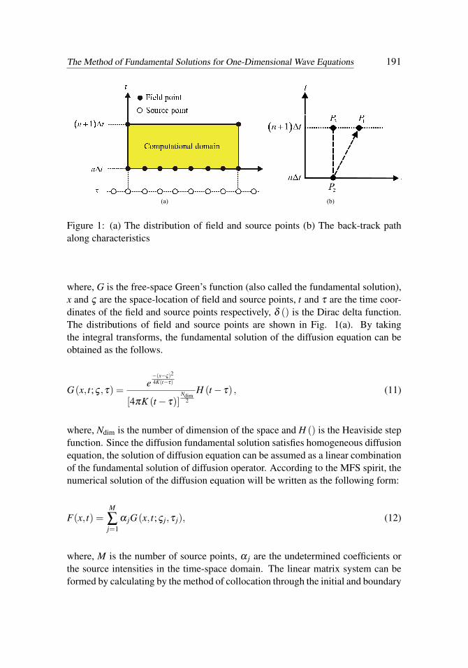
In Fig. 1 (b), the line P2P1 is the characteristic path on which transport of thescalar quantity can be traced. If the wave speed at point P1 is assigned, the spatiallocation of point P2 can be traced by Eq.(9). When the spatial location of point P2 isdetermined, the solutions along characteristics P2P1 will follow the characteristic-diffusion equation according to the material derivative. After the diffusion processis calculated by the MFS, the solution of the advection-diffusion equation can beobtained directly by ELM. In Fig. 1 (b), points P2 and P3 are located at the samespatial position but at different time levels. On the other words, the line P2P3 is thecharacteristics path for describing pure diffusion phenomena. When we solve thediffusion equation, the diffusive result of point P2 at n + 1 level will be calculatedin point P3. If the physical fields have the advection phenomenon, P2P1 is thecharacteristic path which satisfies the advection phenomenon and the physical valueat point P1 is properly replaced by the diffusion results at point P3. And then theresults of the advection-diffusion equations at t = (n+1)∆t thus can be acquired.

3.2 The method of fundamental solutions

The fundamental solution of the diffusion equation is governed by the followingequation.

∂G∂ t

= K∇2G+δ (x− ς)δ (t− τ) , (10)


(a) (b)

Figure 1: (a) The distribution of field and source points (b) The back-track pathalong characteristics

where, G is the free-space Green’s function (also called the fundamental solution),x and ς are the space-location of field and source points, t and τ are the time coor-dinates of the field and source points respectively, δ () is the Dirac delta function.The distributions of field and source points are shown in Fig. 1(a). By takingthe integral transforms, the fundamental solution of the diffusion equation can beobtained as the follows.

G(x, t;ς ,τ) =e−(x−ς)2

4K(t−τ)

[4πK (t− τ)]Ndim

2

H (t− τ) , (11)

where, Ndim is the number of dimension of the space and H () is the Heaviside stepfunction. Since the diffusion fundamental solution satisfies homogeneous diffusionequation, the solution of diffusion equation can be assumed as a linear combinationof the fundamental solution of diffusion operator. According to the MFS spirit, thenumerical solution of the diffusion equation will be written as the following form:

F(x, t) =M

∑j=1

α jG(x, t;ς j,τ j), (12)

where, M is the number of source points, α j are the undetermined coefficients orthe source intensities in the time-space domain. The linear matrix system can beformed by calculating by the method of collocation through the initial and boundary


conditions.

Ai jα j = Bi and Ai j =e

−|xi−ς j|24K(ti−τ j)

[4πK (ti− τ j)]Ndim

2

H (ti− τ j) , (13)

The vector Bi is obtained from the initial and boundary conditions. After solvingthe linear matrix system, the coefficients α j can be obtained. Then the solution ofdiffusion equation can be expressed by Eq. (12).

3.3 The Eulerian-Lagrangian method of fundamental solutions

Following the statement of the ELM and MFS, the solution of the advection-diffusionequation can be written as:

Fn+1i (xn+1

i , t) =M

∑j=1

α jG(xn+1

i −a∆t, t;ς j,τ j), (14)

where, α j are obtained by calculating the initial and boundary conditions. FromEqs. (11)-(14), the physical value Fn+1

i can be easily obtained by the ELMFS.When diffusion effects become very weak (K«1), the advection-diffusion equationcan be considered as the advection equation.

3.4 One-dimensional wave model

According to the D’Alembert formulation, the wave equation can be reduced totwo solutions of advection equation as Φ+ (x−at) and Φ− (x+at). In mesh-dependent method, it is necessary to use the interpolation technique for back track-ing the Φ+ (x−a∆t) and Φ− (x+a∆t) in time-space domain from level (n+1)∆tto level n∆t. The ELMFS is the suitable meshless method to approximate the so-lutions as Φ+ (x−a∆t) and Φ− (x+a∆t) along the characteristics path in the time-space domain with very small diffusion coefficient. After obtaining the solutionsΦ+ (x−at) and Φ− (x+at), the solution of wave equation can be calculated as thefollowing.

ϕn+1 (xn+1

i , t)

= Φ+ (xn+1

i −a∆t)+Φ

− (xn+1i +a∆t

)⇒ ϕ

n+1 (xn+1i , t

)=

M

∑j=1

α jG(xn+1

i −a∆t, t;ς j,τ j)+

M

∑j=1

α jG(xn+1

i +a∆t, t;ς j,τ j)

(15)

Following the definition of the D’Alembert solution and the ELMFS, the numericalprocedures of the proposed meshless model are listed below:


1. Set the suitable initial conditions, Eq. (2).

2. Separate the initial conditions for the two opposite-direction traveling wavesΦ+ and Φ− by the D’Alembert formulation, Eq. (4).

3. Obtain the solutions of two opposite-direction waves by ELMFS, Eqs. (15).

4. Combine the opposite-direction traveling waves by the general solution, Eq.(3), and update the initial condition for next time step.

4 Numerical Experiments

We consider five related numerical experiments to verify the proposed model forsolving the one-dimensional wave problems. The numerical examples are analyzedto prove the idea of the proposed numerical method, and show the advantages ofthe proposed scheme for the infinite and finite domains problems. We will use theroot-mean-square error ERMS to measure the accuracy, which is defined as:

ERMS =

√√√√ 1Np

Np

∑i=1

(ϕi,Numerical−ϕi,Analytical

)2. (16)

4.1 First-order wave propagation

In the first example, the first-order one-dimensional wave propagation problem isselected to reveal the capability of the proposed ELMFS. In this case, this physicalkinematic wave field is governed by the advection or first-order wave equation withthe positive unit wave propagation speed as the following:

∂ϕ

∂ t+

∂ϕ

∂x= 0, −5 < x < 10, t > 0. (17)

The initial condition is written as:

ϕ (x, t)|t=0 =

{sin(x) −π ≤ x≤ π

0 otherwise, (18)

with the following boundary condition:

ϕ (x, t)|x=−5 = 0. (19)

The analytical solution for this problem is shown as follows:

ϕ (x, t) =

{sin(x− t) −π ≤ x− t ≤ π

0 otherwise. (20)


-5 0 5 10x

-1

-0.5

0

0.5

1

φ

t = 0ELMFSAnalytical solution

-5 0 5 10

x

-1

-0.5

0

0.5

1

φ

t = 2.5ELMFSAnalytical solution

(a) (b)

-5 0 5 10x

-1

-0.5

0

0.5

1

φ

t = 6.5ELMFSAnalytical solution

-5 0 5 10

x

-1

-0.5

0

0.5

1

φ


(c) (d)

-5 0 5 10x

-1

-0.5

0

0.5

1

φ


-5 0 5 10

x

-1

-0.5

0

0.5

1

φ


(e) (f)

Figure 2: The wave evolution with 161 points of example 4.1 (a) t = 0 (b) t = 2.5(c) t = 6.5 (d) t = 8 (e) t = 10 (f) t = 12


(a) (b)

(c) (d)

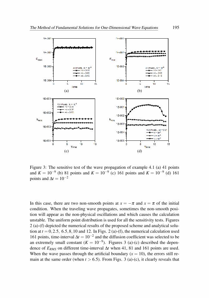
Figure 3: The sensitive test of the wave propagation of example 4.1 (a) 41 pointsand K = 10−9 (b) 81 points and K = 10−9 (c) 161 points and K = 10−9 (d) 161points and ∆t = 10−2

In this case, there are two non-smooth points at x = −π and x = π of the initialcondition. When the traveling wave propagates, sometimes the non-smooth posi-tion will appear as the non-physical oscillations and which causes the calculationunstable. The uniform point distribution is used for all the sensitivity tests. Figures2 (a)-(f) depicted the numerical results of the proposed scheme and analytical solu-tion at t = 0,2.5, 6.5,8,10 and 12. In Figs. 2 (a)-(f), the numerical calculation used161 points, time-interval ∆t = 10−2 and the diffusion coefficient was selected to bean extremely small constant (K = 10−9). Figures 3 (a)-(c) described the depen-dence of ERMS on different time-interval ∆t when 41, 81 and 161 points are used.When the wave passes through the artificial boundary (x = 10), the errors still re-main at the same order (when t > 6.5). From Figs. 3 (a)-(c), it clearly reveals that


as the number of nodes increases, the errors will decrease. In Fig 3 (d), the errorcurves reveal the diffusion coefficient K = 10−9 is small enough to approximatethe advection wave propagation phenomenon. In this sensitivity test, the solutionsare not sensitive to time-interval (∆t) by the ELMFS. From Figs. 3 (b) and (c), theERMS are almost smaller than 10−2. In these results, the solutions show consistentbehavior.

4.2 The Cauchy problem in infinite domain with zero initial velocity

The one-dimensional Cauchy or initial value problem is selected to demonstratethe capability of the proposed model. The unit wave speed is used in this problem.The initial conditions are considered as a smooth function in infinite computationaldomain:

ϕ (x, t)|t=0 = e−x2,

∂ϕ (x, t)∂ t

∣∣∣∣t=0

= 0, −10 < x < 10. (21)

The analytical solution for this problem is displayed as the following.

ϕ (x, t) =12

[e−(x−t)2

+ e−(x+t)2]. (22)

In order to deal with the artificial boundary at x = −10 and x = 10, the boundaryconditions for the Φ+ and Φ− can be written as:

Φ+ (x, t)

∣∣x=−10 = 0 and Φ

− (x, t)∣∣x=10 = 0 (23)

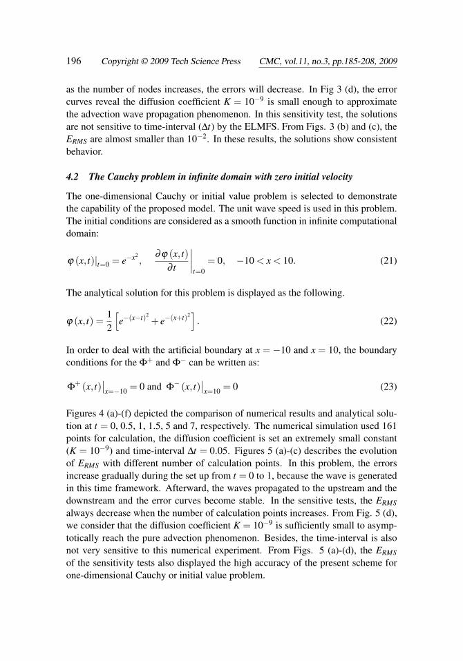
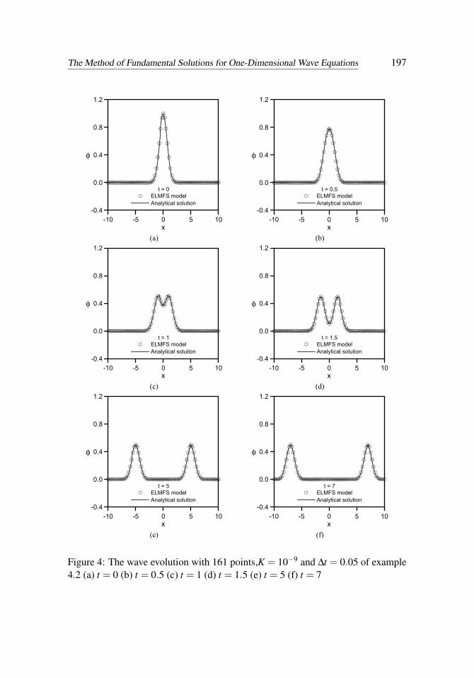
Figures 4 (a)-(f) depicted the comparison of numerical results and analytical solu-tion at t = 0, 0.5, 1, 1.5, 5 and 7, respectively. The numerical simulation used 161points for calculation, the diffusion coefficient is set an extremely small constant(K = 10−9) and time-interval ∆t = 0.05. Figures 5 (a)-(c) describes the evolutionof ERMS with different number of calculation points. In this problem, the errorsincrease gradually during the set up from t = 0 to 1, because the wave is generatedin this time framework. Afterward, the waves propagated to the upstream and thedownstream and the error curves become stable. In the sensitive tests, the ERMS

always decrease when the number of calculation points increases. From Fig. 5 (d),we consider that the diffusion coefficient K = 10−9 is sufficiently small to asymp-totically reach the pure advection phenomenon. Besides, the time-interval is alsonot very sensitive to this numerical experiment. From Figs. 5 (a)-(d), the ERMS

of the sensitivity tests also displayed the high accuracy of the present scheme forone-dimensional Cauchy or initial value problem.


-10 -5 0 5 10x

-0.4

0.0

0.4

0.8

1.2

φ

t = 0ELMFS modelAnalytical solution

-10 -5 0 5 10

x

-0.4

0.0

0.4

0.8

1.2

φ

t = 0.5ELMFS modelAnalytical solution

(a) (b)

-10 -5 0 5 10x

-0.4

0.0

0.4

0.8

1.2

φ


-10 -5 0 5 10

x

-0.4

0.0

0.4

0.8

1.2

φ


(c) (d)

-10 -5 0 5 10x

-0.4

0.0

0.4

0.8

1.2

φ


-10 -5 0 5 10

x

-0.4

0.0

0.4

0.8

1.2

φ


(e) (f)

Figure 4: The wave evolution with 161 points,K = 10−9 and ∆t = 0.05 of example4.2 (a) t = 0 (b) t = 0.5 (c) t = 1 (d) t = 1.5 (e) t = 5 (f) t = 7


(a) (b)

(c) (d)

Figure 5: The sensitive test of the Cauchy problem of example 4.2

(a) 41 points and 910K −= (b) 81 points and 910K −= (c) 161 points and 910K −= (d) 161 points and 0.05tΔ =

Figure 5: The sensitive test of the Cauchy problem of example 4.2 (a) 41 points andK = 10−9 (b) 81 points and K = 10−9 (c) 161 points and K = 10−9 (d) 161 pointsand ∆t = 0.05

4.3 The Cauchy problem in infinite domain with zero initial amplitude

In the third test, the one-dimensional Cauchy or initial value problem is selectedto express the proposed scheme for dealing with the non-zero second kind initialcondition of the wave field. The wave speed a is equal to one for this problem. Theinitial conditions are selected as a smooth function as the following.

ϕ (x, t)|t=0 = 0,∂ϕ (x, t)

∂ t

∣∣∣∣t=0

= xe−x2, −10 < x < 10. (24)

The analytical solution for this problem can be written as follows.

ϕ (x, t) =14

[e−(x−t)2

− e−(x+t)2]. (25)


The artificial boundary conditions at the x = −10 and x = 10 for Φ+ and Φ− arethe same as the case 4.2.

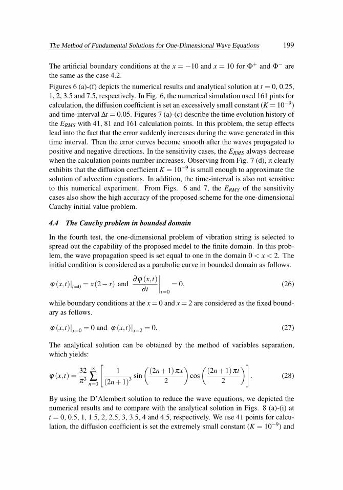
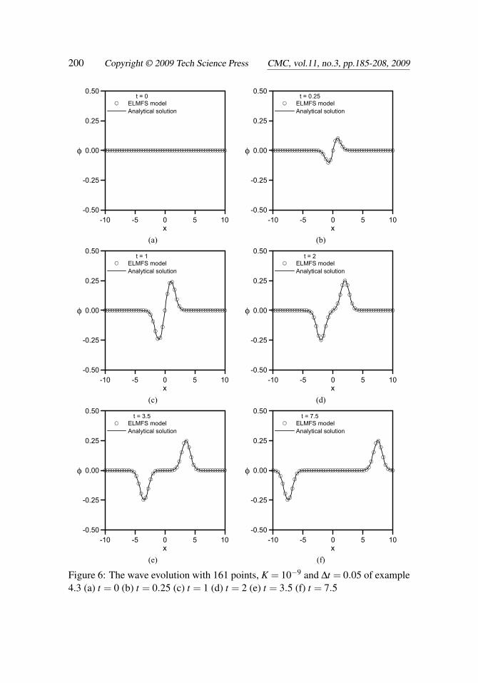
Figures 6 (a)-(f) depicts the numerical results and analytical solution at t = 0, 0.25,1, 2, 3.5 and 7.5, respectively. In Fig. 6, the numerical simulation used 161 pints forcalculation, the diffusion coefficient is set an excessively small constant (K = 10−9)and time-interval ∆t = 0.05. Figures 7 (a)-(c) describe the time evolution history ofthe ERMS with 41, 81 and 161 calculation points. In this problem, the setup effectslead into the fact that the error suddenly increases during the wave generated in thistime interval. Then the error curves become smooth after the waves propagated topositive and negative directions. In the sensitivity cases, the ERMS always decreasewhen the calculation points number increases. Observing from Fig. 7 (d), it clearlyexhibits that the diffusion coefficient K = 10−9 is small enough to approximate thesolution of advection equations. In addition, the time-interval is also not sensitiveto this numerical experiment. From Figs. 6 and 7, the ERMS of the sensitivitycases also show the high accuracy of the proposed scheme for the one-dimensionalCauchy initial value problem.

4.4 The Cauchy problem in bounded domain

In the fourth test, the one-dimensional problem of vibration string is selected tospread out the capability of the proposed model to the finite domain. In this prob-lem, the wave propagation speed is set equal to one in the domain 0 < x < 2. Theinitial condition is considered as a parabolic curve in bounded domain as follows.

ϕ (x, t)|t=0 = x(2− x) and∂ϕ (x, t)

∂ t

∣∣∣∣t=0

= 0, (26)

while boundary conditions at the x = 0 and x = 2 are considered as the fixed bound-ary as follows.

ϕ (x, t)|x=0 = 0 and ϕ (x, t)|x=2 = 0. (27)

The analytical solution can be obtained by the method of variables separation,which yields:

ϕ (x, t) =32π3

∞

∑n=0

[1

(2n+1)3 sin(

(2n+1)πx2

)cos(

(2n+1)πt2

)]. (28)

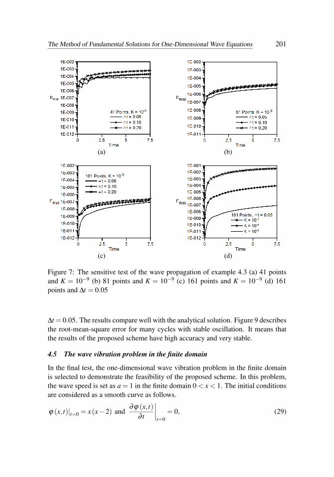
By using the D’Alembert solution to reduce the wave equations, we depicted thenumerical results and to compare with the analytical solution in Figs. 8 (a)-(i) att = 0, 0.5, 1, 1.5, 2, 2.5, 3, 3.5, 4 and 4.5, respectively. We use 41 points for calcu-lation, the diffusion coefficient is set the extremely small constant (K = 10−9) and


-10 -5 0 5 10x

-0.50

-0.25

0.00

0.25

0.50

φ


-10 -5 0 5 10

x

-0.50

-0.25

0.00

0.25

0.50

φ


(a) (b)

-10 -5 0 5 10x

-0.50

-0.25

0.00

0.25

0.50

φ


-10 -5 0 5 10

x

-0.50

-0.25

0.00

0.25

0.50

φ


(c) (d)

-10 -5 0 5 10x

-0.50

-0.25

0.00

0.25

0.50

φ


-10 -5 0 5 10

x

-0.50

-0.25

0.00

0.25

0.50

φ


(e) (f)

Figure 6: The wave evolution with 161 points, K = 10−9 and ∆t = 0.05 of example4.3 (a) t = 0 (b) t = 0.25 (c) t = 1 (d) t = 2 (e) t = 3.5 (f) t = 7.5


(a) (b)

(c) (d)

Figure 7: The sensitive test of the wave propagation of example 4.3

(a) 41 points and 910K −= (b) 81 points and 910K −= (c) 161 points and 910K −= (d) 161 points and 0.05tΔ =

Figure 7: The sensitive test of the wave propagation of example 4.3 (a) 41 pointsand K = 10−9 (b) 81 points and K = 10−9 (c) 161 points and K = 10−9 (d) 161points and ∆t = 0.05

∆t = 0.05. The results compare well with the analytical solution. Figure 9 describesthe root-mean-square error for many cycles with stable oscillation. It means thatthe results of the proposed scheme have high accuracy and very stable.

4.5 The wave vibration problem in the finite domain

In the final test, the one-dimensional wave vibration problem in the finite domainis selected to demonstrate the feasibility of the proposed scheme. In this problem,the wave speed is set as a = 1 in the finite domain 0 < x < 1. The initial conditionsare considered as a smooth curve as follows.

ϕ (x, t)|t=0 = x(x−2) and∂ϕ (x, t)

∂ t

∣∣∣∣t=0

= 0, (29)


0 0.5 1 1.5 2x

-2

-1

0

1

2

φ


0 0.5 1 1.5 2

x

-2

-1

0

1

2

φ


0 0.5 1 1.5 2x

-2

-1

0

1

2

φ


(a) (b) (c)

0 0.5 1 1.5 2x

-2

-1

0

1

2

φ


0 0.5 1 1.5 2

x

-2

-1

0

1

2

φ


0 0.5 1 1.5 2x

-2

-1

0

1

2

φ


(d) (e) (f)

0 0.5 1 1.5 2x

-2

-1

0

1

2

φ


0 0.5 1 1.5 2

x

-2

-1

0

1

2

φ


0 0.5 1 1.5 2x

-2

-1

0

1

2

φ


(g) (h) (i)

Figure 8: The wave evolution with 41 points, K = 10−9 and ∆t = 0.05 of example4.4 (a) t = 0 (b) t = 0.5 (c) t = 1 (d) t = 1.5 (e) t = 2 (f) t = 2.5 (g) t = 3 (h) t = 3.5(i) t = 4.5


0 16 32 48 64Time

1E-009

1E-008

1E-007

1E-006

1E-005

1E-004

1E-003

1E-002

ERMS

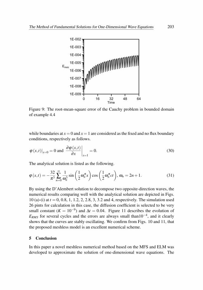
Figure 9: The root-mean-square error of the Cauchy problem in bounded domainof example 4.4

while boundaries at x = 0 and x = 1 are considered as the fixed and no flux boundaryconditions, respectively as follows.

ϕ (x, t)|x=0 = 0 and∂ϕ (x, t)

∂x

∣∣∣∣x=1

= 0. (30)

The analytical solution is listed as the following.

ϕ (x, t) =−32π3

∞

∑n=0

1ω3

nsin(

12

ωπn x)

cos(

12

ωπn ct)

, ωn = 2n+1. (31)

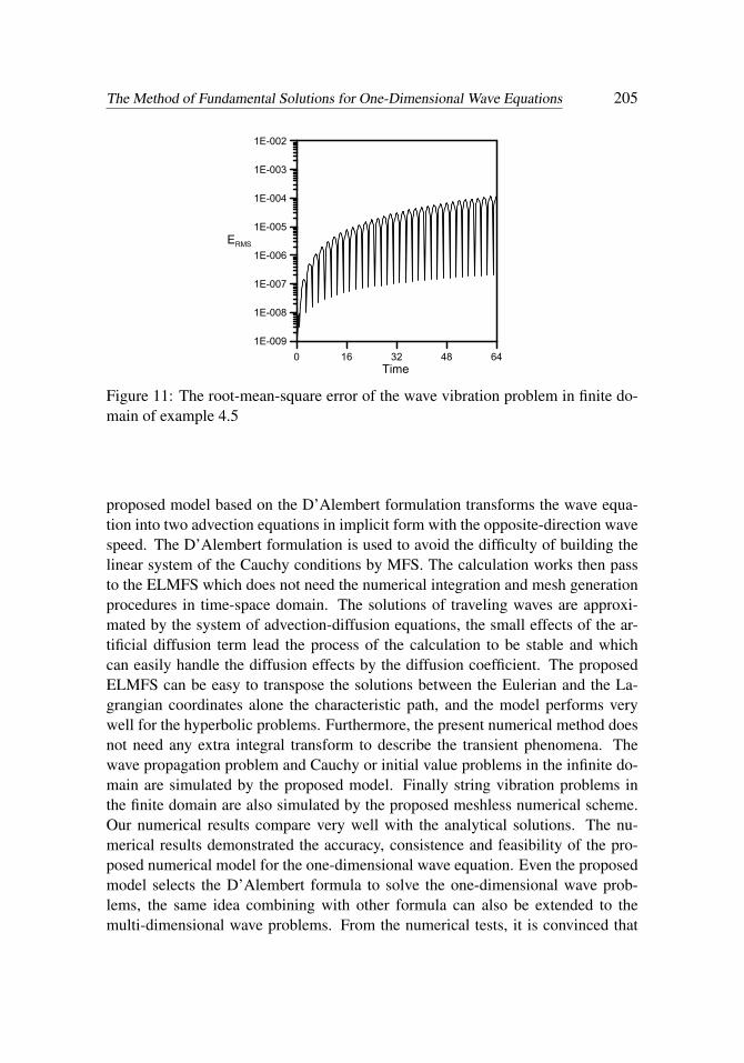
By using the D’Alembert solution to decompose two opposite-direction waves, thenumerical results comparing well with the analytical solution are depicted in Figs.10 (a)-(i) at t = 0, 0.8, 1, 1.2, 2, 2.8, 3, 3.2 and 4, respectively. The simulation used26 pints for calculation in this case, the diffusion coefficient is selected to be verysmall constant (K = 10−9) and ∆t = 0.04. Figure 11 describes the evolution ofERMS for several cycles and the errors are always small than10−4, and it clearlyshows that the curves are stably oscillating. We confirm from Figs. 10 and 11, thatthe proposed meshless model is an excellent numerical scheme.

5 Conclusion

In this paper a novel meshless numerical method based on the MFS and ELM wasdeveloped to approximate the solution of one-dimensional wave equations. The


0 0.2 0.4 0.6 0.8 1x

-1.5

-1

-0.5

0

0.5

1

1.5

t = 0Analytical solutionELMFS model

0 0.2 0.4 0.6 0.8 1

x

-1.5

-1

-0.5

0

0.5

1

1.5

φ

t = 0.8Analytical solutionELMFS model

0 0.2 0.4 0.6 0.8 1x

-1.5

-1

-0.5

0

0.5

1

1.5

φ


(a) (b) (c)

0 0.2 0.4 0.6 0.8 1x

-1.5

-1

-0.5

0

0.5

1

1.5


0 0.2 0.4 0.6 0.8 1

x

-1.5

-1

-0.5

0

0.5

1

1.5

φ


0 0.2 0.4 0.6 0.8 1x

-1.5

-1

-0.5

0

0.5

1

1.5

φ


(d) (e) (f)

0 0.2 0.4 0.6 0.8 1x

-1.5

-1

-0.5

0

0.5

1

1.5


0 0.2 0.4 0.6 0.8 1

x

-1.5

-1

-0.5

0

0.5

1

1.5

φ


0 0.2 0.4 0.6 0.8 1x

-1.5

-1

-0.5

0

0.5

1

1.5

φ


(g) (h) (i)

Figure 10: The wave evolution with 26 points, K = 10−9 and ∆t = 0.04 of example4.5 (a) t = 0 (b) t = 0.8 (c) t = 1 (d) t = 1.2 (e) t = 2 (f) t = 2.8 (g) t = 3 (h) t = 3.2(i) t = 4


0 16 32 48 64Time

1E-009

1E-008

1E-007

1E-006

1E-005

1E-004

1E-003

1E-002

ERMS

Figure 11: The root-mean-square error of the wave vibration problem in finite do-main of example 4.5

proposed model based on the D’Alembert formulation transforms the wave equa-tion into two advection equations in implicit form with the opposite-direction wavespeed. The D’Alembert formulation is used to avoid the difficulty of building thelinear system of the Cauchy conditions by MFS. The calculation works then passto the ELMFS which does not need the numerical integration and mesh generationprocedures in time-space domain. The solutions of traveling waves are approxi-mated by the system of advection-diffusion equations, the small effects of the ar-tificial diffusion term lead the process of the calculation to be stable and whichcan easily handle the diffusion effects by the diffusion coefficient. The proposedELMFS can be easy to transpose the solutions between the Eulerian and the La-grangian coordinates alone the characteristic path, and the model performs verywell for the hyperbolic problems. Furthermore, the present numerical method doesnot need any extra integral transform to describe the transient phenomena. Thewave propagation problem and Cauchy or initial value problems in the infinite do-main are simulated by the proposed model. Finally string vibration problems inthe finite domain are also simulated by the proposed meshless numerical scheme.Our numerical results compare very well with the analytical solutions. The nu-merical results demonstrated the accuracy, consistence and feasibility of the pro-posed numerical model for the one-dimensional wave equation. Even the proposedmodel selects the D’Alembert formula to solve the one-dimensional wave prob-lems, the same idea combining with other formula can also be extended to themulti-dimensional wave problems. From the numerical tests, it is convinced that


the proposed model is a promising wave solver for engineering applications.

Acknowledgement: We would like to dedicate this paper to celebrating the 60th

birthday of Professor Wen-Hwa Chen of the National Tsing-Hua University. TheNational Science Council (NSC) of Taiwan is gratefully acknowledged for provid-ing the financial support to carry out the present work under the grant nos. NSC-95-221-E-002-406 and NSC-95-2221-E-002-26, it is greatly appreciated.

References

Alves, C. J. S.; Antunes, P. R. S. (2005): The method of fundamental solutionsapplied to the calculation of eigenfrequencies and eigenmodes of 2D simply con-nected shapes. CMC: Computers Materials & Continua, vol. 2, pp. 251-265.

Amaziane, B.; Naji, A.; Ouazar, D. (2004): Radial basis function and geneticalgorithms for parameter identification to some groundwater flow problems. CMC:Computers Materials & Continua, vol. 1, pp. 117-128.

Callsen, S.; Estorff, O. V.; Zaleski, O. (2004): Direct and indirect approach ofa desingularized boundary element formulation for acoustical problems. CMES:Computer Modeling in Engineering and Sciences, vol. 6, pp. 421-429.

Chen, J. T.; Chou, K. S.; Kao, S. K. (2009): One-dimensional wave animationusing Mathematica. Comput Appl Eng Educ, vol.17, pp.323-339.

Chen, K. H.; Chen, J. T.; Kao, J. H. (2006): Regularized meshless method forsolving acoustic eigenproblem with multiply connected domain. CMES: ComputerModeling in Engineering and Sciences, vol.16, pp. 27-39.

Chen, K. H.; Chen, J. T.; Kao, J. H. (2008): Regularized meshless method forantiplane shear problems. Int J Numer Meth Eng, vol.73, pp.1251-1273.

Chen, K. H.; Kao, J. H.; Chen, J. T. (2009): Regularized meshless method forantiplane piezoelectricity problems with multiple inclusions. CMC: ComputersMaterials & Continua, vol.9, pp.253-279.

Chen, K. H.; Wu, K. L.; Kao, J. H.; Chen, J. T. (2009): Desingular meshlessmethod for solving Laplace equation with over-specified boundary conditions usingregularization techniques. Comput Mech, vol.43, pp.827-837.

Chen, K. H.; Kao, J. H.; Chen, J. T.; Young, D. L.; Lu, M. C. (2006): Rgularizedmeshless method for multiply-connected—domain Laplace problems. Eng AnalBound Elem, vol.30, pp.882-896.

Golberg, M. A. (1995): The method of fundamental solutions for Poisson’s equa-tion. Eng Anal Bound Elem, vol.16, pp. 205-213.

Godinho, L.; Tadeu, A.; Amado Mendes, P. (2007): Wave Propagation around


Thin Structures using the MFS. CMC: Computers Materials & Continua, Vol. 5,No. 2, pp. 117-128.

Gou, M. H.; Young, D. L. (2005): Application of the method of fundamentalsolutions to solve advection-diffusion equations. The Pacific Congress on MarineScience and Technology, Nov. 6-9, 2005, Changhwa, Taiwan.

Gu, M. H.; Young, D. L.; Fan, C. M. (2008): The meshless method for one-dimensional hyperbolic equation. J Aeronaut Astronaut Aviat (A), vol. 40, pp.63-72.

Han, Z. D.; Atluri, S. N. (2004): A meshless local Petrov-Galerkin (MLPG) ap-proach for 3-dimensional elasto-dynamics. CMC: Computers Materials & Con-tinua, vol. 1, pp. 129-140.

Iske, A.; Käser, M. (2005): Two-phase flow simulation by AMMoC, an adaptivemeshfree method of characteristics. CMES: Computer Modeling in Engineeringand Sciences, vol. 7, pp. 133-148.

Kupradze, V. D.; Aleksidze, M. A. (1964): The method of fundamental solutionsfor the approximate solution of certain boundary value problems. U.S.S.R. ComputMath Math Phys, vol.4, pp. 82-126.

Ma, Q.W. (2007): Numerical Generation of Freak Waves Using MLPG_R andQALE-FEM Methods. CMES: Computer Modeling in Engineering and Sciences,Vol. 18, No. 3, pp. 223-234.

Mathon, R.; Johnston, R. L. (1977): The approximate solution of elliptic boundary-value problem by method of fundamental solutions. SIAM J Numer Anal, vol. 14,pp. 638-650.

Shu, C.; Wu, W. X.; Wang, C. M. (2005): Analysis of metallic waveguides byusing least square-based finite difference method. CMC: Computers Materials &Continua, vol. 2, pp. 189-200.

Sladek, J.; Sladek, V.; Zhang, C.; Garcia, S. F.; Wunsche, M. (2006): Meshlesslocal Petrov-Galerkin method for plane piezoelectricity. CMC: Computers Materi-als & Continua, vol. 4, pp. 109-117.

Tsai, C.C.; Young, D.L.; Fan, C.M.; Chen, C.W. (2006): Time-dependent fun-damental solutions for unsteady stokes problems. Eng Anal Bound Elem, vol. 30,pp. 897-908.

Wazwaz, A. M. (1998): A reliable technique for solving the wave equation in aninfinite one-dimensional medium. Appl Math Comput, vol. 92, pp. 1-7.

Whitham, G. B. (1974): Linear and nonlinear waves. John Wiley & Sons press,New York, pp. 214-215.

Young, D. L.; Ruan, J. W. (2005): Method of fundamental solutions for scattering


problems of electromagnetic waves. CMES: Computer Modeling in Engineeringand Sciences, vol. 7, pp. 223-232.

Young, D. L.; Wang, Y. F.; Eldho, T. I. (2000): Solution of the advection-diffusion equation using the Eulerian-Lagrangian boundary element method. EngAnal Bound Elem, vol. 24, pp. 449-457.

Young, D. L.; Tsai, C. C.; Fan, C. M. (2004): Direct approach to solve nonho-mogeneous diffusion problems using fundamental solutions and dual reciprocitymethods. J Chin Inst Eng, vol. 27, pp. 597-609.

Young, D. L.; Chen, C. S.; Wong, T. K. (2005): Solution of Maxwell’s equationsusing the MQ method. CMC: Computers Materials & Continua, vol. 2, pp. 267-276.

Young, D. L.; Chen, K. H.; Lee, C. W. (2005): Novel meshless method for solvingthe potential problems with arbitrary domain. J Comput Phys, vol. 209, pp. 290-321.

Young, D. L.; Chen, C. W.; Fan, C. M. (2008) The method of fundamental so-lutions for low Reynolds number flows with moving rigid body, in The method offundamental solutions-meshless Method, Eds. C.S. Chen, A. Karageorghis, Y. S.Smyrlis, Dynamic Publishers, USA, pp.181-206.

Young, D. L.; Gu, M. H.; Fan, C. M. (2009) The time-marching method of fun-damental solutions for wave equations. Eng Anal Bound Elem, vol. 33, pp. 1411-1425.

Young, D. L.; Fan, C. M.; Hu, S. P.; Atluri, S. N. (2008): The Eulerian-Lagrangianmethod of fundamental solutions for two-dimensional unsteady Burgers’ equations.Eng Anal Bound Elem, vol. 32, pp. 395-412.

Young, D. L.; Lin, Y. C.; Fan, C. M.; Chiu, C. L. (2009) Method of fundamentalsolutions for solving incompressible Navier-Stokes problems. Eng Anal BoundElem, vol.33, pp.1031-1044.

Young, D. L.; Tsai, C. C.; Murugesan, K.; Fan, C. M.; Chen, C. W. (2004):Time-dependent fundamental solutions for homogeneous diffusion problems. EngAnal Bound Elem, vol. 28, pp. 1463-1473.

Young, D. L.; Fan, C. M.; Tsai, C. C.; Chen, C. W.; Murugesan, K. (2006):Eulerian-Lagrangian method of fundamental solutions for multi-dimensional advection-diffusion equation. Int J Math Forum, vol. 1, pp. 687-706.

the method of fundamental solutions for one-dimensional

Documents