164

APPENDIX A

A – COMPUTATION OF ORGANIC LOADING RATE (OLR)

OLR = COD concentration x flow Rate

Liquid volume of the reactor

A2- Heterogeneous process model

bAbHCbKcA

CbHbKb

HbμAZbKz

ZbCbKc

KcSbKs

SbηgμHCbKoH

CbSbKs

SbμHrX

A3 – Effluen substrate concentration

c1T

Cdo

θKY)θK(1SSe

do

e1T

C

KSSKY

θ1

baseOECEa10baseOEa9baseCEa8OECEa7

basea6OEa5CEa4basea3.a2.OEa1.CEa0X 222

165

Appendix B

Hartree-Lowry and Modified Lowry Protein Assays

Considerations for use

The Lowry assay (1951) is an often-cited general use protein assay. For some time it

was the method of choice for accurate protein determination for cell fractions,

chromatography fractions, enzyme preparations, and so on. The bicinchoninic acid

(BCA) assay is based on the same princple and can be done in one step, therefore it

has been suggested (Stoscheck, 1990) that the 2-step Lowry method is outdated.

However, the modified Lowry is done entirely at room temperature. The Hartree

version of the Lowry assay, a more recent modification that uses fewer reagents,

improves the sensitivity with some proteins, is less likely to be incompatible with

some salt solutions, provides a more linear response, and is less likely to become

saturated. The Hartree-Lowry assay will be described first.

Principle

Under alkaline conditions the divalent copper ion forms a complex with peptide bonds

in which it is reduced to a monovalent ion. Monovalent copper ion and the radical

groups of tyrosine, tryptophan, and cysteine react with Folin reagent to produce an

unstable product that becomes reduced to molybdenum/tungsten blue.

Equipment

In addition to standard liquid handling supplies a spectrophotometer with infrared

lamp and filter is required. Glass or polystyrene (cheap) cuvettes may be used.

166

Procedure - Hartree-Lowry assay

Reagents

1. Reagent A consists of 2 gm sodium potassium tartrate x 4 H20, 100 gm sodium

carbonate, 500 ml 1N NaOH, H20 to one liter (that is, 7mM Na-K tartrate,

0.81M sodium carbonate, 0.5N NaOH final concentration). Keeps 2 to 3

months.

2. Reagent B consists of 2 gm 2 gm sodium potassium tartrate x 4 H20, 1 gm

copper sulfate (CuSO4 x 5H20), 90 ml H20, 10 ml 1N NaOH (final

concentrations 70 mM Na-K tartrate, 40 mM copper sulfate). Keeps 2 to 3

months.

3. Reagent C consists of 1 vol Folin-Ciocalteau reagent diluted with 15 vols water.

Assay

1. Prepare a series of dilutions of 0.3 mg/ml bovine serum albumin in the same

buffer containing the unknowns, to give concentrations of 30 to 150

micrograms/ml (0.03 to 0.15 mg/ml).

2. Add 1.0 ml each dilution of standard, protein-containing unknown, or buffer

(for the reference) to 0.90 ml reagent A in separate test tubes and mix.

3. Incubate the tubes 10 min in a 50 degrees C bath, then cool to room

temperature.

4. Add 0.1 ml reagent B to each tube, mix, incubate 10 min at room temperature.

5. Rapidly add 3 ml reagent C to each tube, mix, incubate 10 min in the 50 degree

bath, and cool to room temperature. Final assay volume is 5 ml.

6. Measure absorbance at 650 nm in 1 cm cuvettes.

Analysis

167

Prepare a standard curve of absorbance versus micrograms protein (or vice versa), and

determine amounts from the curve. Determine concentrations of original samples from

the amount protein, volume/sample, and dilution factor, if any.

Procedure - modified Lowry (room temperature)

Reagents

1. Dissolve 20 gm sodium carbonate in 260 ml water, 0.4 gm cupric sulfate (5x

hydrated) in 20 ml water, and 0.2 gm sodium potassium tartrate in 20 ml water.

Mix all three solutions to prepare the copper reagent.

2. Prepare 100 ml of a 1% solution (1 gm/100 ml) of sodium dodecyl sulfate

(SDS).

3. Prepare a 1 M solution of NaOH (4 gm/100 ml).

4. For the 2x Lowry concentrate mix 3 parts copper reagent with 1 part SDS and 1

part NaOH. Solution is stable for 2-3 weeks. Warm the solution to 37 degrees C

if a white precipitate forms, and discard if there is a black precipitate. Better,

keep the three stock solutions, and mix just before use.

5. Prepare 0.2 N Folin reagent by mixing 10 ml 2 N Folin reagent with 90 ml

water. Kept in an amber bottle, the dilution is stable for several months.

Assay

1. Dilute samples to an estimated 0.025-0.25 mg/ml with buffer. If the

concentration can't be estimated it is advisable to prepare a range of 2-3

dilutions spanning an order of magnitude. Prepare 400 microliters each dilution.

Duplicate or triplicate samples are recommended.

2. Prepare a reference of 400 microliters buffer. Prepare standards from 0.25

mg/ml bovine serum albumin by adding 40-400 microliters to 13 x 100 mm

tubes + buffer to bring volume to 400 microliters/tube.

168

3. Add 400 microliters of 2x Lowry concentrate, mix thoroughly, incubate at room

temp. 10 min.

4. Add 200 microliters 0.2 N Folin reagent very quickly, and vortex immediately.

Complete mixing of the reagent must be accomplished quickly to avoid

decomposition of the reagent before it reacts with protein. Incubate for 30 min.

more at room temperature.

5. Use glass or polystyrene cuvettes to read the absorbances at 750 nm. If the

absorbances are too high, they may be read at 500 nn.

Comments

Recording of absorbances need only be done within 10 min. of each other for this modified

procedure, whereas the original Lowry required precise timing of readings due to color

instability. This modification is less sensitive to interfering agents and is more sensitive to

protein than the original. As with most assays, the Lowry can be scaled up for larger cuvette

sizes, however more protein is consumed. Proteins with an abnormally high or low percentage

of tyrosine, tryptophan, or cysteine residues will give high or low errors, respectively.

169

APPENDIX C

Fig. C1 (a) The SEM of biomass (VSS) of Synthetic Municipal wastewater

170

Fig. C1 (a) The SEM of Biomass (VSS) of Municipal wastewater (field)

EDAX spectra and elemental composition

171

172

Fig. C 1 ‘GC’ of feed

Fig. C 2 ‘MS’ of feed at retention time (RT) - 1.45 seconds

173

Fig. C 3 ‘MS’ of feed at RT- 4.45 seconds

Fig. C 4 ‘MS’ of feed at RT- 4.53 seconds

174

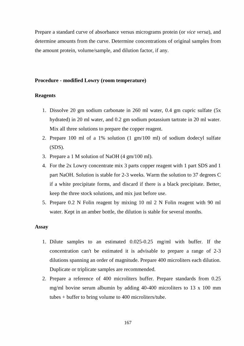
Fig. C 5 ‘MS’ of feed at RT- 5.92 seconds

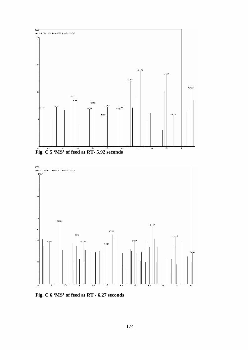
Fig. C 6 ‘MS’ of feed at RT - 6.27 seconds

175

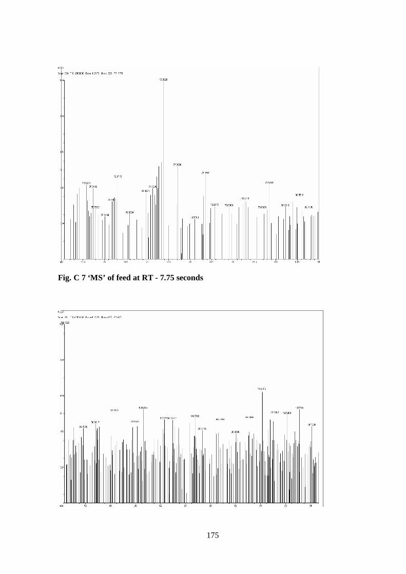
Fig. C 7 ‘MS’ of feed at RT - 7.75 seconds

176

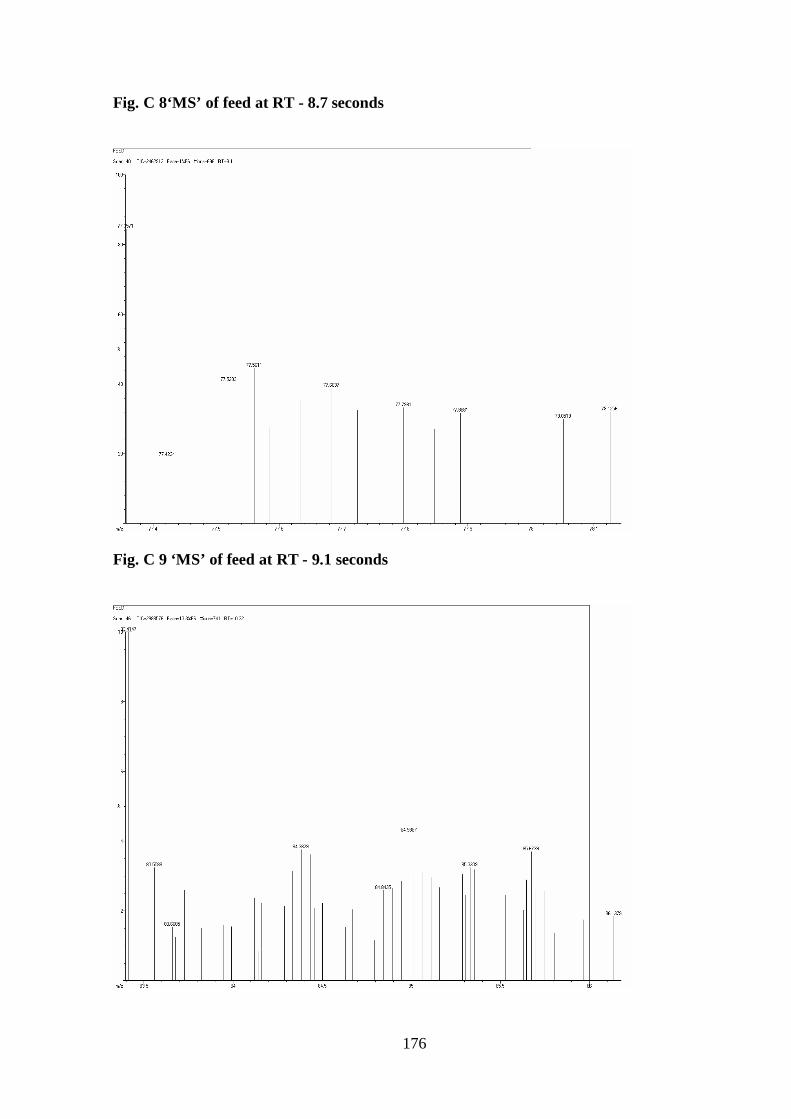
Fig. C 8‘MS’ of feed at RT - 8.7 seconds

Fig. C 9 ‘MS’ of feed at RT - 9.1 seconds

177

Fig. C 10 ‘MS’ of feed at RT - 10.32 seconds

Fig. C 11 ‘MS’ of feed at RT - 10.32 seconds

178

Fig. C 12 ‘MS’ of feed at RT - 10.32 seconds

Fig. C 13 ‘MS’ of feed at RT - 11.67 seconds

179

Fig. C 14 ‘MS’ of feed at RT - 11.67 seconds

Fig. C 15 ‘MS’ of feed at RT - 14.9 seconds

180

Fig. C 16 ‘MS’ of feed at RT - 15.02 seconds

Fig. C 17 ‘GC’ of permeate for maximum OLR at 24 h HRT

181

Fig. C 18 ‘MS’ of permeate for maximum OLR, 24 h HRT detected at RT - 2.32 seconds

182

Fig. C 19 ‘MS’ of permeate for maximum OLR, 24 h HRT detected at RT - 2.4 seconds

Fig. C 20 ‘MS’ of permeate for maximum OLR, 24 h HRT detected at RT - 3.88 seconds

183

Fig. C 21 ‘MS’ of permeate for maximum OLR, 24 h HRT detected at RT - 5.27 seconds

Fig. C 22 ‘MS’ of permeate for maximum OLR, 24 h HRT detected at RT - 5.84 seconds

184

Fig. C 23 ‘MS’ of permeate for maximum OLR, 24 h HRT detected at RT - 5.96 seconds

Fig. C 24 ‘MS’ of permeate for maximum OLR, 24 h HRT detected at RT - 5.96 seconds

185

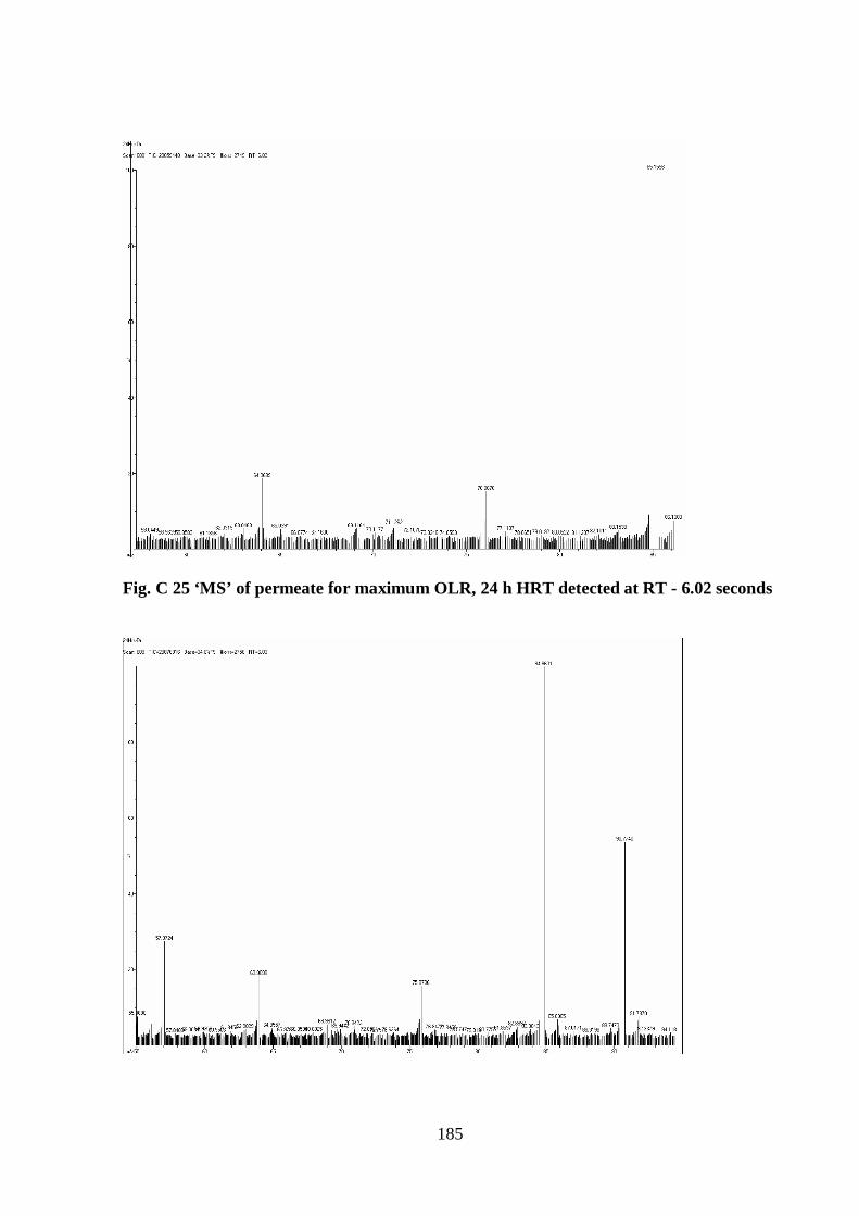
Fig. C 25 ‘MS’ of permeate for maximum OLR, 24 h HRT detected at RT - 6.02 seconds

186

Fig. C 26 ‘MS’ of permeate for maximum OLR, 24 h HRT detected at RT - 6.03 seconds

Fig. C 27 ‘MS’ of permeate for maximum OLR, 24 h HRT detected at RT - 6.05 seconds

187

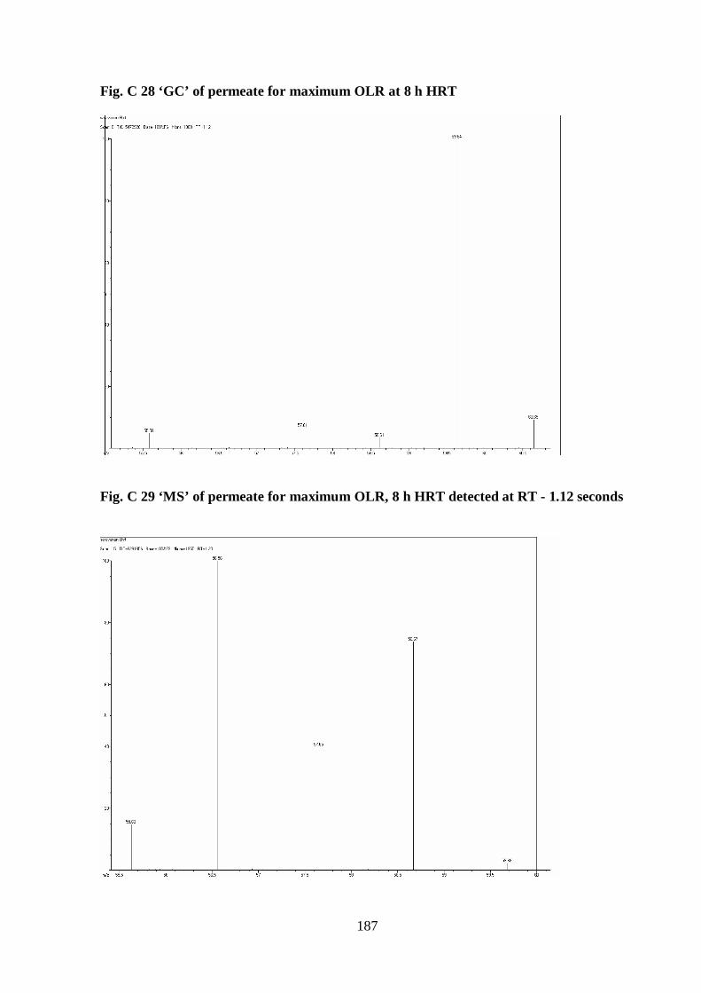
Fig. C 28 ‘GC’ of permeate for maximum OLR at 8 h HRT

Fig. C 29 ‘MS’ of permeate for maximum OLR, 8 h HRT detected at RT - 1.12 seconds

188

Fig. C 30 ‘MS’ of permeate for maximum OLR, 8 h HRT detected at RT - 1.23 seconds

Fig. C 31 ‘MS’ of permeate for maximum OLR, 8 h HRT detected at RT - 2.28 seconds

189

Fig. C 32 ‘MS’ of permeate for maximum OLR, 8 h HRT detected at RT - 3.3 seconds

APPENDIX D B1 SCANNING ELECTRON MICROSCOPY (SEM)

For SEM the sludge sample (containing microorganisms on the membrane) was first

fixed by soaking in phosphate buffered 6% glutaraldehyde solution for 1 hour at less

than 20°C, washed with phosphate buffer and then dehydrated with acetone. The

detailed procedure is given below.

B2 MEDIA USED FOR ABOVE PROCEDURE

Monobasic sodium phosphate solution (0.25M):

27.6 g of NaH2PO4.H2O or 31.21 g NaH2PO4.2H2O was dissolved in distilled water

and made upto 100 ml.

190

Dibasic sodium phosphate solution (0.2M):

3.561 g Na2HPO4.2H2O or 53.65 g Na2HPO4.7H2O was dissolved in distilled water

and made upto 100ml.

Phosphate buffer 0.2 M (pH = 7.9):

30.5 ml of (2) above was made upto 19.5 ml of (1) above.

Phosphate buffer 0.1 M (pH = 7):

50 ml of (3) above was made upto 100 ml with distilled water.

27.5 mg/L of calcium chloride was added to (4) above.

Phosphate buffered glutaraldehyde fixative (6%)

(i) 0.2 M phosphate buffer : 50 ml

(ii) 25% gluteraldehyde in distilled water : 24 ml

(iii) Distilled water : 26 ml

(Glutaraldehyde fixative was prepared fresh and stored in clean glass stopper bottle).

B3 SAMPLE PREPARATION FOR SEM

After passing the required media following steps were adopted for preparing the

samples for SEM.

Step 1: Fixation schedule

1. An appropriate volume of sludge sample was taken in test tube.

2. An equal volume of 6% glutaraldehyde fixative mix was added, gently shaking

or tipping the tube simultaneously.

191

3. The tube was kept for fixation (fixation time = 1h at < 20 C) in a refrigerator

say approximately at 19 C.

4. The sample was centrifuged after fixation.

Step 2: Washing

The fixed sample was washed in 0.1 M phosphate buffer for 2h. buffer contained 27.5

mg/L calcium chloride. The contents were kept at 4 C during washing.

Step 3: Dehydration of fixed sample

Dehydration was accomplished by passing the fixed sample specimen through a

graded series of solutions of increasing concentration of dehydrating agent (ethanol or

acetone) in water, ending with pure dehydrating agent. During the dehydration, while

one solution was removed carefully with a fine pipette or a syringe, the next one was

poured on. Care was taken to ensure that, the volume of solution used was at least 10

times the volume of specimen. Dehydration was done with gradual increase in

temperature so that 90-95% strength solutions were obtained at room temperature.

Dehydration schedule: 50% ethanol in water - 10 minutes

70% ethanol in water - 10 minutes

95% ethanol in water - 10 minutes

100% ethanol - 15 minutes

The sample was then scanned using a scanned using Scanning Electron Microscope.

192

APPENDIX E

The algorithms used in the ODE solvers vary according to order of accuracy

(Shampine , 1994) and the type of systems (stiff or nonstiff) they are designed to

solve.

Different solvers accept different parameters in the options list. For more information,

see odeset and Integrator Options in the MATLAB Mathematics documentation.

Parameters ode45 ode23 ode113 ode15s ode23s ode23t ode23tb

RelTol, AbsTol,

NormControl

√ √ √ √ √ √ √

OutputFcn, OutputSel,

Refine, Stats

√ √ √ √ √ √ √

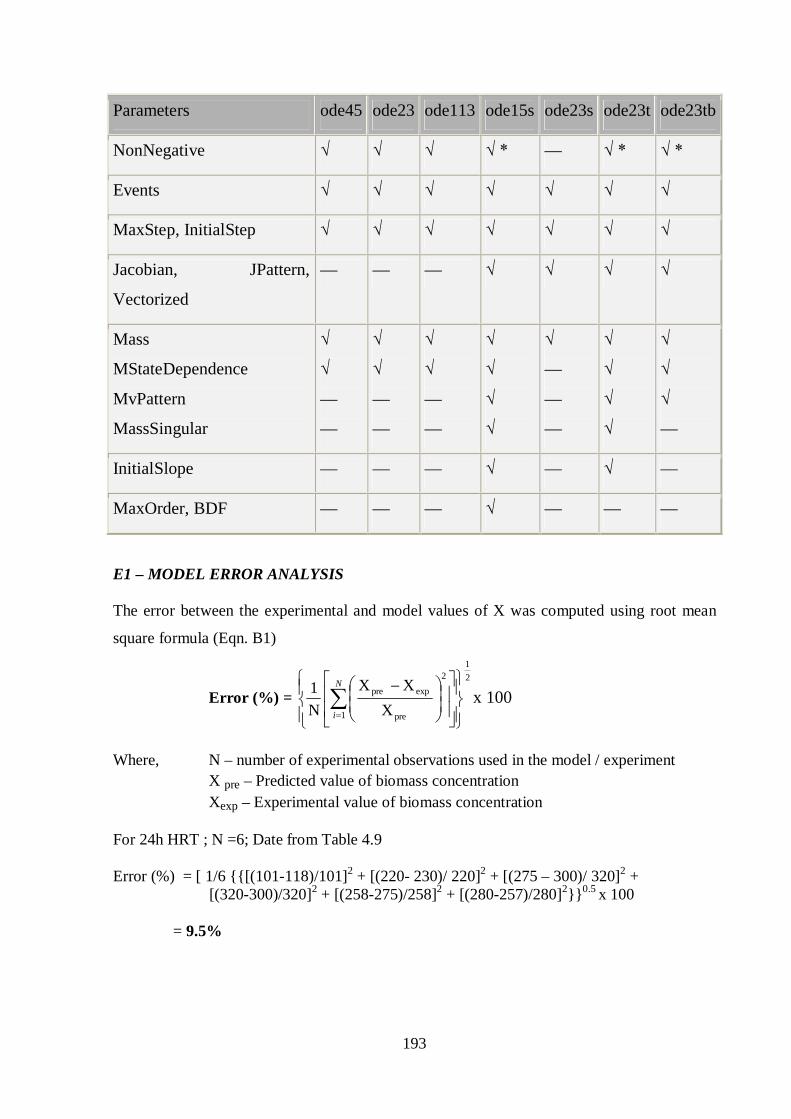
193

Parameters ode45 ode23 ode113 ode15s ode23s ode23t ode23tb

NonNegative √ √ √ √ * — √ * √ *

Events √ √ √ √ √ √ √

MaxStep, InitialStep √ √ √ √ √ √ √

Jacobian, JPattern,

Vectorized

— — — √ √ √ √

Mass

MStateDependence

MvPattern

MassSingular

√

√

—

—

√

√

—

—

√

√

—

—

√

√

√

√

√

—

—

—

√

√

√

√

√

√

√

—

InitialSlope — — — √ — √ —

MaxOrder, BDF — — — √ — — —

E1 – MODEL ERROR ANALYSIS The error between the experimental and model values of X was computed using root mean

square formula (Eqn. B1)

Error (%) = 21

1

2

pre

exp pre

XXX

N1

N

ix 100

Where, N – number of experimental observations used in the model / experiment X pre – Predicted value of biomass concentration Xexp – Experimental value of biomass concentration For 24h HRT ; N =6; Date from Table 4.9 Error (%) = [ 1/6 {{[(101-118)/101]2 + [(220- 230)/ 220]2 + [(275 – 300)/ 320]2 + [(320-300)/320]2 + [(258-275)/258]2 + [(280-257)/280]2}}0.5 x 100 = 9.5%

194

LIST OF PUBLICATIONS BASED ON THE RESEARCH WORK

(A) International Journal/(s)

1. Balasubramanian, S., and R. Saravanane (2010), On-line monitoring of

active biomass concentration in wastewater treatment plant using a

conductometric microbial biosensor, Sustainable Environmental research,

20 (5), 311-315.

2. Balasubramanian, S., and R. Saravanane (2009), Development of

conductometric detection and quantification of microbial biomass for

monitoring operational performance of a wastewater treatment plant, Water

Science and Technology (accepted).

(B) International Conferences

1. Balasubramanian, S., and R. Saravanane (2009) Development of conductometric

biosensor for monitoring microbial biomass in biological treatment system, 10th

IWA specialist conference on Instrumentation control and Automation, 14-17,

June 2009, Cairns, Australia.

2. Balasubramanian, S., and R. Saravanane (2009), On-line monitoring of active

biomass concentration in wastewater treatment plant using a conductometric

microbial biosensor, The 3rd IWA – ASPIRE conference, 18th – 22nd, October,

2009, Taiwan.

3. Balasubramanian, S., and R. Saravanane (2008), Conceptual biosensor model

for assessment and on-line monitoring of bacteriological quality in Urban and

rural water supply and wastewater schemes, Proceedings of international

workshop on “Indo/French technologies for sustainable Environment”, 10th

April 2008, Pondicherry Engineering College, Puducherry, India,

Intercultural Network for development and peace (INDP), India and

Poitou Charentes Region, France, pp. 78-85.