the mechanics of precision presplitting
TRANSCRIPT

Scholars' Mine Scholars' Mine
Doctoral Dissertations Student Theses and Dissertations
Fall 2019
The mechanics of precision presplitting The mechanics of precision presplitting
Anthony Joseph Konya
Follow this and additional works at: https://scholarsmine.mst.edu/doctoral_dissertations
Part of the Civil Engineering Commons, and the Explosives Engineering Commons
Department: Mining Engineering Department: Mining Engineering
Recommended Citation Recommended Citation Konya, Anthony Joseph, "The mechanics of precision presplitting" (2019). Doctoral Dissertations. 2836. https://scholarsmine.mst.edu/doctoral_dissertations/2836
This thesis is brought to you by Scholars' Mine, a service of the Missouri S&T Library and Learning Resources. This work is protected by U. S. Copyright Law. Unauthorized use including reproduction for redistribution requires the permission of the copyright holder. For more information, please contact [email protected].
THE MECHANICS OF PRECISION PRESPLITTING
by
ANTHONY JOSEPH KONYA
A DISSERTATION
Presented to the Faculty of the Graduate School of the
MISSOURI UNIVERSITY OF SCIENCE AND TECHNOLOGY
In Partial Fulfillment of the Requirements for the Degree
DOCTOR OF PHILOSOPHY
in
EXPLOSIVE ENGINEERING
2019
Approved by:
Dr. Paul Worsey, Advisor Dr. Kyle Perry
Dr. Gillian Worsey Dr. Cesar Mendoza
Dr. Braden Lusk

2019
Anthony Joseph Konya
All Rights Reserved

iii
ABSTRACT
Precision Presplitting is a widely used method of presplit blasting for the mining
and construction industries. In recent years considerable effort has gone into the
development of empirical equations based on field data to be able to better design the
Precision Presplit for various rock types and structural environments. However, the most
widely discussed theory about the mechanics of the presplit formation, that of shockwave
collisions, does not appear to be applicable for this method of presplitting.
This research has disproven this theory based on insufficient magnitude of the
shockwave from modeling with basic wave mechanics. Other authors have suggested
alternative theories based on the gas pressurization of the borehole. Recently the concept
of hoop stresses as a result of the gas pressurization of the borehole was suggested. No
method to analyze the gas pressurization of the borehole and magnitude of the hoop
stresses existed. This research seeks to develop the basic theory to determine the hoop
stress field for a Precision Presplit blast, using basic laws from thermodynamics and
mechanics of materials to present a mathematical proof to determine the borehole
pressure from a decoupled charge and the magnitude of the hoop stress developed in the
rock.
This modelling approach analyzes the stress from both the shockwave and gas
pressure, which are quantified and compared to the tensile strength of the rock. This
research shows that the shockwave magnitude is much too low to cause presplit
formation while the hoop stress has sufficient magnitude to cause the split.

iv
ACKNOWLEDGMENTS
The author wishes to express his gratitude to his advisor, Dr. Paul Worsey, for his
advice, assistance, and encouragement throughout the author’s schooling and this project;
to Dr. Gillian Worsey for her ongoing support and encouragement through the authors
schooling and this project; to Dr. Kyle Perry for his assistance and valued ideas in
preparation on this project; to Dr. Cesar Mendoza for his support and encouragement on
this project; and to Dr. Braden Lusk for his support and encouragement on this project.
The author also wishes to express gratitude to the Missouri University of Science
and Technology and the Mining Engineering and Explosive Engineering programs for
ongoing education without which this project would not have been possible. The author
also wishes to thank the Missouri S&T Curtis Laws Wilson Library, Interlibrary Loan
Services.
The author also wishes to express sincere gratitude to Precision Blasting Services
for allowing the author to utilize equipment and unpublished research which were vital to
the completion of this project.
The author wishes to express his gratitude to Dr. Calvin J. Konya, without whom
none of this would have been possible. The mentorship and knowledge imparted has been
the basis for the author’s current and ongoing work.
v
TABLE OF CONTENTS
Page
ABSTRACT ....................................................................................................................... iii
ACKNOWLEDGMENTS ................................................................................................. iv
LIST OF ILLUSTRATIONS ............................................................................................. ix
LIST OF TABLES ............................................................................................................. xi
NOMENCLATURE ........................................................................................................ xiii
SECTION
1. INTRODUCTION ........................................................................................................ 1
2. REVIEW OF LITERATURE ....................................................................................... 6
2.1. INTRODUCTION OF BLASTING TECHNIQUES ......................................... 6
2.2. HISTORIC MECHANICS OF BREAKAGE..................................................... 8
2.3. SHOCK BREAKAGE IN COMMERCIAL BLASTING ................................ 17
2.3.1. The Discovery of Shockwaves. .............................................................. 17
2.3.2. Shockwave Research in Commercial Blasting. ...................................... 20
2.3.2.1. Livingston Cratering Theory. ....................................................22
2.3.2.2. U.S. Bureau of Mines Cratering Theory. ...................................26
2.3.2.3. Shockwave Spallation Theory. ..................................................27
2.3.2.4. Strain Wave Theory. ..................................................................32
2.3.2.5. Refutation of the application of shockwaves in blasting. ..........33
2.3.3. Shockwave Theory and Mathematical Concepts. .................................. 37
2.4. GAS PRESSURIZATION BREAKAGE IN COMMERCIAL BLASTING ... 40

vi
2.4.1. Becker-Kistiakowsky-Wilson (BKW) Equation of State ....................... 45
2.4.2. Cook’s Equation of State. ....................................................................... 48
2.4.3. Taylor’s Equation of State. ..................................................................... 49
2.4.4. Outoyne-Skidmore-Konya (OSK) Equation of State. ............................ 49
2.4.5. Theoretical Borehole Pressure Calculations. ...........................................51
2.5. PRESPLITTING ............................................................................................... 52
2.5.1. Traditional Presplitting. .......................................................................... 58
2.5.2. Precision Presplitting. ..............................................................................59
2.5.3. Propellant Presplitting. .............................................................................69
3. EMPIRICAL ANALYSIS OF BOREHOLE PRESSURES ....................................... 71
3.1. DEVELOPMENT OF AN EMPIRICAL BOREHOLE PRESSURE MODEL ............................................................................................................ 71
3.2. MODIFICATION OF THE EMPIRICAL MODEL ........................................ 76
3.3. EMPIRICAL MODEL FOR TYPICAL PRECISION PRESPLIT .................. 81
4. THEORETICAL ANALYSIS OF BOREHOLE PRESSURES ................................. 82
4.1. INTRODUCTION TO THEORETICAL MODELS ........................................ 82
4.1.1. Temperature of Detonation. ................................................................... 83
4.1.2. Specific Heats for Explosive Products. .................................................. 84
4.1.2.1. Dulong-Petit Limit. ....................................................................85
4.1.2.2. PETN detonation products. ........................................................86
4.1.2.3. Specific heat for nitrogen, N2. ...................................................87
4.1.2.4. Specific heat of water vapor, H2O. ............................................87
4.1.2.5. Specific heat for carbon dioxide, CO2. ......................................88
4.1.2.6. Specific heat for carbon monoxide, CO.....................................88
vii
4.1.3. Calculation of the Temperature of the Explosion. ................................. 93
4.2. DETONATION PRESSURE MODEL ............................................................ 98
4.2.1. Validation of Equations of State from Experimental Data..................... 98
4.2.2. Development of Detonation Pressure Model from Taylor EOS. ......... 102
4.3. DEVELOPMENT OF THERMODYNAMIC MODEL ................................ 106
4.4. COMPARISON OF PRESSURE MODELS .................................................. 123
4.5. BOTTOM CHARGE EFFECTS .................................................................... 127
4.6. PRESSURE OF A TYPICAL PRECISION PRESPLIT ................................ 131
5. HOOP STRESS MODEL FOR BLASTING ............................................................ 132
5.1. DEVELOPMENT OF HOOP STRESS MODEL .......................................... 132
5.2. SIMPLIFICATION OF HOOP STRESS MODEL ........................................ 140
5.3. HOOP STRESS OF A PRECISION PRESPLIT BLAST .............................. 141
6. MAGNITUDE OF THE SHOCKWAVE FROM PRESPLITTING ........................ 147
6.1. SHOCKWAVE MECHANICS ...................................................................... 147
6.2. SHOCKWAVE MAGNITUDE FOR A PRECISION PRESPLIT ................ 148
7. RESULTS AND DISCUSSION ............................................................................... 151
8. CONCLUSIONS....................................................................................................... 155
APPENDICES
A. CALCULATIONS OF BOREHOLE PRESSURE FOR PETN .....................156
B. PRECISION PRESPLIT BOREHOLE PRESSURE ......................................166
C. VALIDATION OF ISOTHERMAL ASSUMPTION ....................................188

viii
D. CIRCUMFERENTIAL STRESSES AROUND A BOREHOLE…….………..193
BIBLIOGRAPHY ........................................................................................................... 196
VITA ................................................................................................................................207
ix
LIST OF ILLUSTRATIONS
Page
Figure 2.1 – 90° conical crater from an explosive charge placed at point L .................. 11
Figure 2.2 – Dual-Cratering Theory ............................................................................... 13
Figure 2.3 – Shearing Theory from a plan view looking downward on the bench with point ‘b’ as the blasthole .................................................................... 14
Figure 2.4 – Crater after Livingston (erroneously) showing shock breakage ................. 25
Figure 2.5 – Hino research on unconfined charges......................................................... 28
Figure 2.6 – Initial conditions of shockwave breakage model ....................................... 35
Figure 2.7 – Detonation for shockwave breakage model ............................................... 35
Figure 2.8 – Shockwave can be seen in plexiglass as darkened ring .............................. 36
Figure 2.9 – Shockwave spallation occurring at 15% of typical burden ........................ 36
Figure 2.10 – Final frame of test series showing magnitude of gas breakage (internal) versus shock breakage (external) .............................................. 37
Figure 2.11 – Pressure in the bore of a cannon from various propellants after Nobel .......................................................................................................... 43
Figure 2.12 – Borehole pressure from high explosives after Otuonye ............................. 44
Figure 2.13 – First test of a Precision Presplit completed in 1980 ................................... 61
Figure 2.14 – Decoupling ratio to borehole pressure ........................................................ 66
Figure 2.15 – Precision Presplit blast completed in 4 different rock types in Grundy, Virginia ........................................................................................ 67
Figure 2.16 – Precision Presplit load variations based on typical values for specific rock type........................................................................................ 68
Figure 3.1 – Explosive load to borehole pressure for large decoupling in a two-inch diameter hole ............................................................................... 75
Figure 3.2 – Borehole pressure variations of explosive load with constant borehole diameter ....................................................................................... 79

x
Figure 3.3 – Borehole pressure variations based on borehole diameter at constant explosive loads ............................................................................. 80
Figure 4.1 – Specific heat at constant volume for nitrogen with variations in temperature using three data sets................................................................ 89
Figure 4.2 – Specific heat at constant volume for water vapor with variations to temperature using three data sets ........................................................... 90
Figure 4.3 – Specific heat at constant volume for carbon dioxide with variations to temperature using three data sets ........................................................... 91
Figure 4.4 – Specific heat at constant volume for carbon monoxide with variations to temperature using one data set .............................................. 92
Figure 4.5 – Comparison of Equation 28 and Equation 48 to the measured borehole pressures .................................................................................... 111
Figure 4.6 – Comparison of Equation 29 and Equation 49 for borehole pressures from a typical Precision Presplit .............................................................. 112
Figure 4.7 – The basic effects of decoupling ratio on the borehole pressure ............... 113
Figure 4.8 – Thermodynamics pressure model to the measured borehole pressure data from Otuonye ..................................................................... 121
Figure 4.9 – Linear regression analysis for the compressibility as a function of explosive load for PETN explosive .......................................................... 122
Figure 4.10 – Comparison of borehole pressure models at typical Precision Presplit explosive loads .......................................................................... 125
Figure 4.11 – Comparison of borehole pressure models for large explosive loads ........ 126
Figure 4.12 – Borehole pressure as a function of borehole length showing the effects of the bottom load with a column load of 500 grains per foot ..... 130
Figure 5.1 – Hoop stress field as a function of the distance constant (A) .................... 137
Figure 5.2 – The effect of spacing between boreholes on the hoop stress field magnitude ................................................................................................. 138
Figure 5.3 – Variations of hoop stress magnitude to borehole diameter halfway between the boreholes .............................................................................. 139
Figure 5.4 – Magnitude of hoop stress field near the borehole .................................... 145
Figure 5.5 – Magnitude of the hoop stress field farther from the borehole .................. 146
xi
LIST OF TABLES
Page
Table 2.1 – Measured peak pressure for PETN in borehole simulation device after Otuonye ........................................................................................................ 46
Table 2.2 – Pressures from propellants pressure edited to psi ........................................ 47
Table 2.3 – Konya Presplit Factor for various rocks ...................................................... 63
Table 2.4 – Properties of black powder compared to Pyrodex ....................................... 70
Table 2.5 – Tests completed with propellant presplit v. dynamite ................................. 70
Table 3.1 – Borehole pressures compared to charge weight per foot ............................. 72
Table 3.2 – Decoupling ratio for Otuonye work ............................................................. 73
Table 3.3 – Boreholes pressures for Precision Presplitting based on explosive load…………………………………………………………………………………………………. 81
Table 4.1 – Heat of combustion for PETN ..................................................................... 86
Table 4.2 – Calculation of specific heat for first run of explosive temperature ............. 93
Table 4.3 – Calculation for temperature of explosion for the first run ........................... 94
Table 4.4 – Calculation of specific heat for second run of explosive temperature ......... 95
Table 4.5 – Calculation for temperature of explosion second run .................................. 96
Table 4.6 – Calculation of specific heat for second run of explosive temperature ......... 96
Table 4.7 – Calculation for temperature of explosion third run ..................................... 97
Table 4.8 – Explosive gas detonation pressure calculations for various EOS .............. 100
Table 4.9 – Charge volume calculations ....................................................................... 100
Table 4.10 – Pressure calculations for decoupled charge from base equations of state ........................................................................................................ 101
Table 4.11 – Mole fractions for gases produced from PETN ......................................... 114
Table 4.12 – Calculation of reduced temperature of PETN gas mixture ........................ 115
xii
Table 4.13 – Calculation of the reduced pressure, iteration 1 ........................................ 116
Table 4.14 – Calculation of reduced pressure, iteration 2 .............................................. 117
Table 4.15 – Calculation of reduced pressure, iteration 3 .............................................. 118
Table 4.16 – Typical explosive column load for various rock types .............................. 127
Table 5.1 – Typical explosive loads for various rock types ......................................... 142
Table 5.2 – Equivalent explosive loads for various tock types ..................................... 142
Table 5.3 – Comparison of hoop stress at maximum split distance to rock tensile strength ................................................................................... 143
Table 7.1 – Stresses from Precision Presplitting at one borehole diameter from charge ................................................................................................ 152
Table 7.2 – Stresses from Precision Presplitting at maximum split distance ............... 153

xiii
NOMENCLATURE
Symbol Description
W Weight of Charge
B Burden
s Periphery of the Chamber
G Shear Modulus
Pg Gas Pressure in Borehole
Ir Reflected Intensity Constant
It Transmitted Intensity Constant
D Detonation Velocity
PCJ Detonation Pressure
vs Sonic Velocity
ρ Density
b Co-Volume
Te Temperature of Explosion
R Gas Constant
n Inverse Average Molecular Weight
Pe Explosive Pressure
ni Moles of Product Divided by Kg of Explosive
Qe Heat of Explosion
Ve Specific Volume of Explosive Gases
Ng Total Moles of Gaseous Product per Kilogram

xiv
Zc Compressibility
Pc Critical Pressure
Tc Critical Temperature
Pr Reduced Pressure
Tr Reduced Temperature
r Radius
ro External Radius
ri Internal Radius
po External Pressure
pi Internal Pressure
σc Hoop Stress in Circumferential Direction
E Young's Modulus
K Konya Presplit Factor
S Spacing
ni Moles of Product Divided by Kg of Explosive
1
1. INTRODUCTION
Explosives are utilized in both the mining and construction industries for effective
and cost-efficient rock excavation. The majority of the explosives used in both of these
industries is for production blasting, which is defined as the fragmentation of rock and for
mass rock excavation. This type of blasting typically leads to breakage behind the final
row of blastholes, termed overbreak or backbreak, which is acceptable in the main body
of the excavation but is of major concern when blasting near final excavation limits.
In the construction industry the final excavation limit, often called the ‘neat line’,
is specifically designed to produce a stable slope, which minimizes risk of rockfall to the
public or nearby infrastructure. These are typically long-term slopes and any additional
overbreak can result in accelerated weathering of the material, increasing the risk of
rockfall and requiring rework of the area to stabilize the slope.
In addition to stability of slopes, many projects require pouring of concrete next to
the rock wall to build infrastructure such as locks and dams. In these situations, when
blasting does not reach the neat line, mechanical excavation and scaling would be
required to achieve the final wall. These methods are extremely expensive and time
consuming. However, blasting beyond this neat line would result in additional concrete to
fill any areas of overbreak, which also results in large increases in cost and time.
In the mining industry, engineers design pits with an overall pit slope to minimize
the risk of large-scale slope failures. These slopes are designed primarily based on the
natural rock for where the slope is excavated. However, if poor blasting methods are
utilized and the rock behind the slope is fractured, then the designers will often ‘lay the
2
slope back’ or use a shallower slope to protect against a slope failure. This typically
requires the mining of additional waste material, which significantly increases the total
cost of the mine and reduces profitability. In today’s mining industry, mines are looking
to mine deeper, and as a result need to have steeper and more stable slopes, with minimal
backbreak to reduce the risk of a slope failure, significantly improving the safety of
workers and equipment in the pit and increasing the profitability of the mine.
The mining industry also designs bench angles, which is the angle of an
individual bench, to minimize the risk of rockfalls to workers in the mine. Currently
numerous methods exist to protect workers including (1) the design of the bench angle to
minimize the risk of rockfalls, (2) the use of catch benches to stop material from falling
further into the pit, (3) the use of berms to keep rock from reaching work areas and to
keep workers out of areas where rock may fall, (4) the use of mechanical scaling of walls
to reduce the risk of rockfalls, and (5) the use of overbreak control measures in the
blasting process.
The measures used to protect workers all have advantages and disadvantages,
which includes the effectiveness of the particular measure, cost to perform, and reliability
of the measure. The first three methods are effective to reduce the risk in the design of the
mine but are extremely expensive as all lead to mining much larger amounts of waste or
missing ore reserves. Method four cannot be viewed as a legitimate method which is
relied upon, as it does not ensure that the risk of rockfalls are mitigated. This is due to the
inability to reliably scale several benches in a surface mining operation. Instead it would
be viewed as a preventative maintenance method, which should be performed to mitigate
the risk of major rockfalls. Method five increases the operational costs of a site but
3
eliminates the need for mining additional waste and/or missing ore. The use of overbreak
control to generate smooth walls and minimize rockfalls is also a highly reliable method
of mitigating these risks for both short-term and long-term stability. Larger mining
operations have traditionally utilized a combination of all these methods to optimize the
economics for the life of mine.
The ability for a mining or construction project to generate smooth walls using
explosives is paramount to the operation being economically effective and safe for
employees. The use of proper presplitting can reduce the amount of scaling required to
1/10 of that required when traditional blasting is utilized (Paine, Holmes, & Clark, 1961).
This has large economic savings in reduction of manpower and equipment required and
increased excavation capacity. This also leads to a safer project, as less rockfalls occur
during the scaling process when men and equipment are near the highwall. The
minimization of backbreak is not only seen on the face of the excavation, but the
reduction in blast damage is meters thick where proper presplits show no degradation of
the rock beyond the presplit line (Matheson & Swindells, 1981).
While traditional presplit methods can be utilized in hard rock types, they do not
perform properly when they are applied to weaker rocks. This has led to a false concept
that weaker sandstones, shales, mudstones, and siltstones cannot be presplit. However,
the method of Precision Presplitting has been applied to all of these rock types effectively
and shown presplits with near perfect walls in full-scale construction projects (Spagna,
Konya, & Smith, 2005). Traditional presplit methods often caused problems with weaker
types of rock, as the explosive load is too great and crushing or cratering around the
borehole causes overbreak.
4
Oftentimes, the structural properties of the geology being blasted also causes
backbreak beyond the presplit lines (Worsey, Farmer, & Matheson, 1981; Worsey & Qu,
1987). The solution to minimize the effects of these geologic conditions is to bring the
borehole spacing closer together. Traditional presplit design would use a ‘split-factor’ to
adjust the explosive load based on a linear relationship with spacing. However, the
explosive load to spacing relationship is not linear (Konya & Konya, 2017b) and this
leads to overloading of the charge in the area. With this being completed in poor geologic
conditions, oftentimes with heavy jointing and bedding, the presplit will generate
overbreak for the entire region and cause joints and bedding planes to open up from gas
penetration.
The mechanisms behind a presplit formation are not well understood and false
theories are still introduced and propagated by groups and individuals that are not well
read in previous literature and tests. The shock breakage theory is still widely taught and
studied (International Society of Explosive Engineers, 2016; Salmi & Hosseinzadch,
2014) even though this theory has numerous studies showing how it is not applicable and
is a false concept (Konya C. , 1973; Worsey P. , 1981). In fact, under this theory methods
such as Precision Presplitting could not work to produce a presplit.
A new theory is that the explosive generated gases in a borehole causes a hoop
stress field, which causes the presplit fracture to occur (Konya & Konya, 2017a). This
indicates that very small explosive loads could be used, depending on the rock type and
structural environment, to generate a fracture without causing any overbreak to the
surrounding structure. It is proposed that this hoop stress field is a function of the gas
pressure, and the research in this dissertation focuses on defining this gas pressure in a
5
borehole from both detonating and deflagrating explosives to determine if borehole
pressures are possible to generate these hoop stress fields. This dissertation will also
focus on the development of a hoop stress model to determine the magnitude of the stress
field generated from the borehole pressure.
This thesis analyzes both the shockwave breakage and hoop stress theories to
determine the magnitudes of these stresses. This is then compared to various rock
properties such as the Brazilian Tensile Strength. The design of the explosive load for a
Precision Presplit round based on the tensile strength of the rock is also developed. The
models developed and applied are tested against measured borehole pressures. These
models are then applied to actual field conditions to confirm applicability of the models
and to prove that these theoretical models properly explain why the field conditions
occur.
6
2. REVIEW OF LITERATURE
2.1. INTRODUCTION OF BLASTING TECHNIQUES
The use of explosives in rock blasting began on February 8, 1627 in the
Oberbiberstollen of Schemnitz in Hungary which was designed and fired by Caspar
Weindl (Guttmann, 1892) utilizing black powder. With the success of this first blast, the
Hungarian Mine Tribunal quickly disseminated this information throughout Hungary and
the utilization of explosives in underground mining spread so that by 1673 the technology
had spread throughout the Hungarian underground mining industry (Brown E. M., 1673).
Blasting then spread throughout the world where it was introduced in Germany in 1700
and Sweden in 1724 for blasting in the mining industry. With the massive improvements
in rock fragmentation, especially in hard rock, which could not be mined previously
except with fires, the construction industry soon began employing the use of black
powder blasting. The first underground construction tunnel developed with the use of
blasting is documented to have occurred in 1679 to develop the Malpas Tunnel in
Languedoc, France and by 1696 blasting had begun to be used for surface blasting in the
construction industry for the development of roadways on the Abula Pass in Switzerland
(Guttmann, 1892).
Since explosives first began being used in mining and construction, engineers and
scientists have been developing theories to better understand how these explosives work
to break rock, in an attempt to improve the efficiency of blasting (Guttmann, 1892).
These efficiency improvements have been in ways to improve explosives through
chemical formulations and manufacturing processes (Quinan, 1912), develop ways to

7
better design blasts to increase fragmentation and heaving of the muckpile, and to reduce
the environmental factors of blasting; such as ground vibration and overbreak of blasts
(Brown E. M., 1673). The overbreak of a blast, or breakage beyond the design line, has
been of concern since these early construction projects, as overbreak often leads to
raveling of rock and incompetent walls. This overbreak can also cause increases in the
speed of weathering and water penetration behind the slope which can lead to slope
failures. In projects where concrete is used this overbreak requires the additional use of
concrete, which can increase project costs by millions. This is also of concern in
underground workings where poor blasting along the perimeter of the blast will lead to
large pieces of rock hanging on the back and ribs of the excavation, which become
immediately dangerous to workers in the area and add significant cost to remove or bolt.
In an effort to prevent overbreak a technique known as presplitting was
introduced and worked by breaking a smooth line between holes in the rock (Paine,
Holmes, & Clark, 1961). The use of this technique began before explosives were ever
introduced into construction; in places such as Egypt wooden wedges where soaked with
water and placed in boreholes, heated with fire which caused expansion, which formed a
split between boreholes. In northern climates rock was broken in a similar manner; where
boreholes could be filled with water, the water was then frozen, and cracks occurred
between the holes in the winter. This would create large, smooth blocks that could be
used in construction and leave a smooth back wall. Both of these ancient techniques
involved drilling close boreholes and applying a pressure inside of the borehole to cause
fractures between holes. In ancient times this pressure was often slow building, and in
some cases would takes months to fully split the rock (Konya C. , 2015).

8
It was not until the 1950s, that the first explosive presplitting was utilized on the
Lewiston Power Plant (Langefors & Kihlstrom, 1973) as part of the Niagara Powder
Project. In order to accomplish this, boreholes would be drilled from 12’ to 52’,
depending on the bench height, and loaded with detonating cord and partial cartridges of
dynamite. These boreholes were 3 inches in diameter and fired before the main blast,
with all presplit holes being fired at the same time utilizing instantaneous delays. This
produced excellent results and essentially eliminated all overbreak on the project. This
technique has since had widespread use in the mining and explosive industry to minimize
overbreak from explosive blasting. However, while practical rules of thumb exist for
designing blasts in a few specific situations, a deep understanding of the mechanics of
presplitting is lacking and widely debated.
If an explosive applies a pressure to fragment rock in production blasting, the
same pressure must also be responsible for providing the work to break the presplit.
Presplitting uses similar explosives to production blasting which exert similar pressures,
just to a lesser extent, compared to production blasting. Therefore, the background and
understanding of the application of pressure from commercial explosives and the
mechanics of breakage in production blasting are critical to understanding the pressures
applied in presplit blasting.
2.2. HISTORIC MECHANICS OF BREAKAGE
Black powder was the first explosive applied to the breakage of rock in mining
and construction. Black powder is now known as a low explosive, meaning that it fires
slower than the speed of sound in the material. This is often called deflagration and can

9
be considered a slower burning process, which does not result in a shockwave being
generated in the explosive. The pressure profile of black powder is considered one of a
slow build, where the gas pressure in the borehole slowly increases until the powder is
fully consumed, then the pressure is released through either breakage of the rock and
flow through the newly generated cracks or the stemming releases and the gas pressure
vents through the top of the borehole. Various mixtures of black powder would burn at
different rates, which would change the application of this gas pressure; today it is
understood that this would change both the peak pressure generated in the borehole and
the impulse in the borehole. At this time, the gas pressure was the only pressure that was
developed in the borehole and as such was the only work mechanism. This led explosive
engineers of the day to focus on ensuring that the maximum gas pressure was utilized and
contained in the borehole. This introduced tamping, or the filling of the end of a borehole
with inert materials to contain the gas pressure, in 1685 (Guttmann, 1892). Similar
methods to tamping or as we call it today, stemming, are still employed today in mining
and construction operations around the world.
The rate of deflagration in propellants was large and controversy existed on the
quality of black powder for commercial use (Hutton, 1778). At the time it was believed
that the military used better black powder, which burned at a faster rate and applied
greater gas pressures. There was also a major cost difference between black powder
which was made for military use and black powder which was made for commercial
blasting use. This inferior black powder would generate less heave than the higher quality
black powder. From this we can ascertain that the speed at which the gas pressure would
build up would have very real, practical effects on the blasting (Burgoyne, 1874).
10
The world utilized only black powder explosives for over 227 years until 1854,
when gun-cotton was first manufactured in Austria. The gun-cotton plant was quickly
closed however due to numerous explosions during manufacturing. Around a similar
time, Sobrero invented nitroglycerin in 1846 for use as a medicine for angina pectoris. In
1867, Alfred Nobel then invented dynamite with a combination of nitroglycerin and
kieselguhr; inventing the first commercial high explosive. Later Nobel would combine
nitroglycerin and gun-cotton to make gelatin dynamite and give miners the ability to use
these explosives in almost all situations where rock breakage was required. Both
explosives are today considered high explosives, as they detonate faster than the speed of
sound in the material. This produces a high-pressure shockwave, which is then followed
by a rapid increase in gas pressure. This gas pressure build-up is much faster than black
powder and at a much higher temperature due to the increased speed of application and
larger volume of gas generated.
Before the invention of high explosives, numerous rules governed the use of black
powder in the explosives industry. Some of these rules focused on the charge length
where the length of black powder used should be greater than six times the diameter, yet
less than twelve times the diameter. Due to the mechanical aspects of drilling a borehole,
short holes were also used. If a hole was placed vertically into the rock, with only the
surface as relief, the borehole would eject a 90° conical crater (Burgoyne, 1874).
With the reduced amount of black powder which could effectively be used in a
blast and limitations on drilling, this cratering was likely prevalent and does indeed occur
and is seen in work completed nearly a century later (Ash R. , 1974; Livingston C. ,
1961). While this cratering mechanism is still used today, it is not an ideal breakage
11
mechanism from either a performance or an economic standpoint. This theory on
breakage had widespread impacts on how blasting was performed from 1627 to the late
1800s where bench corners were shot under the dual-crater theory.
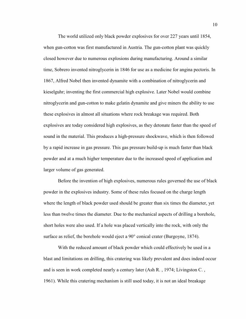
Figure 2.1 - 90° conical crater from an explosive charge placed at point L (Guttmann, 1892)
The dual-crater theory was the idea that the distance from L to M (Figure 2.1) was
the least resistance in the shot, which is described as the shortest distance from the charge
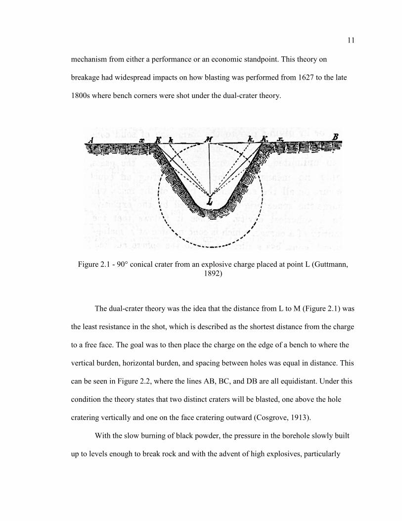
to a free face. The goal was to then place the charge on the edge of a bench to where the
vertical burden, horizontal burden, and spacing between holes was equal in distance. This
can be seen in Figure 2.2, where the lines AB, BC, and DB are all equidistant. Under this
condition the theory states that two distinct craters will be blasted, one above the hole
cratering vertically and one on the face cratering outward (Cosgrove, 1913).
With the slow burning of black powder, the pressure in the borehole slowly built
up to levels enough to break rock and with the advent of high explosives, particularly
12
dynamites, this pressure was applied much more rapidly to the borehole walls. Shortly
after the advent of dynamite researchers began noticing that all of the rules associated
with black powder, such as charge length, did not hold up for dynamite. The prevalent
belief was that this may be due to a different breakage mechanism that was causing
dynamite to break better than black powder. It was then found that when boreholes were
loaded with a high explosive, decoupled, and had full confinement that the borehole
would increase in size, in some cases to double the size of the originally drilled hole,
around the charge.
This led to the theory of borehole springing, which stated that when a high
explosive was utilized, the rapid pressure on the borehole walls would cause compression
in the surrounding rock mass, creating a larger borehole. When the borehole was fully
loaded this large borehole springing effect would cause the borehole to open large
enough that it would move and displace all the rock in-front of it due to crushing actions
and momentum of movement (Guttmann, 1892).
This springing was also utilized then to compensate for the lack of advance in drilling
technology. The boreholes were loaded with small explosive charges and fired, opening
larger diameter boreholes in the rock mass. These would then be fully loaded and fired
again, as a workaround to small drillholes. This greatly increased drilling efficiency back
in the early 1900s. This borehole springing is exhibited still today and the use of
springing was used even in the 1970s to develop larger boreholes in hard rocks such as
those found in Sweden (Langefors & Kihlstrom, 1973).
13
Figure 2.2 - Dual-Cratering Theory (Cosgrove, 1913)
Research later discovered that while this borehole springing was a popular
theoretical concept it did not seem to work in the practical world, as it did not properly
account for the cohesive strength of the rock, it did not properly calculate the force in the
borehole, and it did not account for the relationship between the explosive charge and the
free face. Additionally, drilling technology advanced and then longer and larger diameter
boreholes could be used in the blast. Longer holes resulted in a large increase in borehole
utilization. This was the major downfall of the springing theory, it relied on many of the
similar principles of the cratering theory, particularly in using medium length holes, short
charges, and large amounts of tamping (stemming). With the explosive engineer now able
to use longer holes and fill a larger percentage of the borehole with explosive, it was
evident that springing was not causing breakage. Additionally, it was seen that on these
longer, highly utilized holes which were loaded with high explosives, the breakage was

14
not occurring through conical cratering but was instead breaking through the face, with
no observation of cratering in the vertical direction of the blast. This was the first
realization of the directionality of long charges when aligned with a free face, which was
achieved through a long, slender charge instead of a concentrated ‘spherical’ charge
(Daw & Daw, 1898).
This led to the advent of the shearing theory, which stated that when a charge was
detonated the rock around borehole would shear away from the borehole in a direction of
least resistance, opening up an 80° to 110° crater. This theory stated that “the rock is
most economically and conveniently mined in benches with a straight and vertical wall,
and that the height of such steps depends on the depth and diameter adopted for the
boreholes” (Daw & Daw, 1898).
Figure 2.3 - Shearing Theory from a plan view looking downward on the bench with point ‘b’ as the blasthole (Daw & Daw, 1898)

15
The belief behind the shearing theory was that if a charge was placed at point b,
with the closest distance to relief being W, the lines ab and bc would shear and the rock
wedge would be pushed out due to the gas pressure (Figure 2.3). This was due to the
large gas pressure generated by the charge and then as the rock was thrown forward it
would bend and break into smaller fragments. This was one of the first real developments
of an equation to determine the various dimensions in blasting, which was the
determination of W called the “Line of Resistance,” now known as Burden (B).
Previously the only method to determine the line of resistance was the use of
Hauser’s Law (modified to current blasting terminology), which was an empirical
equation developed regardless of the breakage theory. This equation was extremely poor
in dealing with changes in explosive power. The constant “C” was an empirical
coefficient which can range from 0.02 to 0.50, depending on the strength of a rock.
𝑊𝑊 = 𝐶𝐶𝐵𝐵3 (1)
where W is the weight of the charge in kilograms, C is a constant, and B is the burden in
meters.
Daw and Daw then developed an equation using static loading of ice and the
shearing theory to provide a new equation for determination of Burden.
𝑃𝑃𝑔𝑔 = 𝑠𝑠𝐵𝐵𝑠𝑠 (2)
where Pg was the borehole pressure in psi, s was the shear strength of the rock in psi, B
was the burden in feet, and G was the volume of the chamber in cubic inches. The units
in Equation 1 and 2 are the original units as reported by the respective authors.
At this time, all breakage theories relied solely on the gas pressure causing the
breakage in rock. The gas pressure was a well-established principle which was
16
understood easily. Additionally, engineers and scientists did not understand the
mechanisms of shockwave and had minimal instrumentation to accurately quantify this
occurring from the explosive. However, they did understand that there was a difference
and attributed it to the rapid development of gas pressure from dynamite when compared
to black powder. At the time, gas pressure was the only pressure that was understood to
occur from an explosion, and as such the majority of testing of explosives occurred
through the use of mortar testing. It has been easy to calculate the volumes of gas that is
formed from a gas mixture based on STP, for centuries, however the difficulty in the
development of pressure models was to determine what the temperature of the explosion
was, which had dramatic impacts on the results of the pressure. Additionally, with long
slender charges the velocity of detonation was another difficulty.
It was mathematically determined that gunpowder would produce a pressure of
approximately 85,000 psi. This was then used as a baseline to determine total pressure
developed by the various dynamites using a weight-equivalent testing procedure. When
using bulk explosives, gun powder was then considered the baseline and had an energy
factor of 1.00; therefore, dynamite had a total energy factor of 4.23 meaning that the
dynamite was considered over four times stronger than gunpowder (Andre, 1878). This
increase in power was theorized to be both from the increase in speed of reaction
resulting in a faster force application over a long charge, and in a higher heat of
detonation.
The theory of gas pressurization continued well into the beginning of the 20th
century and was rapidly expanding as explosive engineers of the time attempted to design
explosives to increase the maximum pressure in a blasthole (Quinan, 1912). With the

17
beginning of the World Wars, many explosive engineers and researchers changed their
course of research from application of explosives in rock blasting to military applications.
However, those still working in rock blasting from 1910 to 1950 progressively advanced
the practical application of the gas pressurization theory, focusing efforts on maximizing
the borehole pressure (Roscoe, 1924; Taylor J. , 1945). With the advent of nuclear
weaponry and significant research into increasing the power of weapons systems, a new
method of damage from explosives began being explored in the early 1940s, i.e. shock
breakage.
2.3. SHOCK BREAKAGE IN COMMERCIAL BLASTING
Shockwaves began in the industries as a solely theoretical concept which was not
applied to rock blasting. However, as new research was completed shockwaves quickly
became a major research area in commercial blasting.
2.3.1. The Discovery of Shockwaves. Black powder was one of many rapidly
burning chemicals that existed in the ancient world, yet it was the most popular because
its application as a propellant for firearms was quickly recognized (Bacon, 1733) and by
1314 it was recorded being utilized in multiple battles. While black powder combusts
very rapidly it does not detonate, instead it deflagrates producing no shockwave. It was
not until 1608 that the first high-explosive (Croll, 1609), one that combusts faster than the
speed of sound in the material, was invented. The combustion of this high-explosive
produces a strong shockwave. In 1659 the first ammonium nitrate compound was
produced (Kirk & Othmer, 1947), which today is recognized as a high explosive and is
the dominant ingredient in commercial explosives. Fulminating Silver was then
18
introduced in 1786 (Berthollet, 1786) and Potassium Chlorate followed shortly after
(Kapoor, 1970). These compounds were all considered ‘primary explosives’ or those
which were too sensitive or powerful for practical use. At the time, the inventors of these
compounds had no method to measure the rate at which they combusted, nor did they
understand the difference between a deflagration and detonation.
The shockwave which is produced by high explosives and high velocity impacts
is unique in terms of wave mechanics, magnitude, and velocity. The origins of the
shockwave are developed from acoustical wave theory which was introduced in the mid-
1700s (Le Rond D'Alembert, 1747; De Lagrange, 1781). As mathematical theory of
acoustic (sound) waves progressed, mathematicians attempted to discover the “size of
disturbances” of sound waves, or the intensity of the sound. At this time, it was noted that
“the following disturbances could accelerate the propagation of the preceding ones, in
such a way that the higher the sound the greater is its speed…” (Euler, 1759). This would
help to develop the theory that the speed of a wave depends on its intensity, which is one
of the foundational principles of today’s understanding of shockwaves. The initial
mathematical theory of acoustic waves was the fully developed by 1802 (Biot, 1802).
This acoustical wave theory was then expanded to mathematically incorporate
waves of much greater pressures and much faster speeds than typical acoustic waves
(Poisson, 1808). This was the first mathematical proof of the existence of shockwaves.
Work continued following this in the theory of these waves through the 1800s, but these
waves could not be created easily without detonation (Weber & Weber, 1825). The shock
wave was observed with sharp boundaries in air and termed the shock wave, using sparks
in air (Toepler, 1864), which eventually led to the application of the laws of conservation

19
of mass, conservation of momentum, and conservation of energy to the shockwave. Then
the mathematical proof of a planar shock wave (Christoffel, 1877b) and the propagation
of shock waves through an elastic solid medium (Christoffel, 1877a) was developed.
The first real laboratory tests utilized linear percussion techniques to observe the
formation of a shockwave (Mach & Somner, 1877). A theoretical treatise addressing the
linear relationship between pressure and specific volume of a gas was developed and
termed the “Rayleigh Line” (Rayleigh L. J., 1877). In 1881 gaseous explosive mixtures
were utilized to prove that a shockwave was produced as a result of a detonation
(Berthelot, 1892; Berthelot, 1881). This research first discussed this wave as an
‘explosive wave’ but was later determined to be the shock wave seen in other
applications. This explosive wave was observed to have effects comparable to a sound
wave, except with high active energy and large pressure.
This led to the development of a general theory of discontinuous one-dimensional
flow using Lagrangian coordinates (Hugoniot, 1887), which led to the development of the
Rankine-Hugoniot equations. This along with the Rayleigh line gave researchers a
mathematical method to determine the pressure and velocity of the shockwave.
The first theory of detonation based on shockwaves was completed to
mathematically prove how explosives produce these shockwaves (Mikhel'son, 1893).
This was then investigated and further developed to show that during the detonation of
the explosive, a shockwave first propagates through the medium, which is followed by a
combustion wave (Jouguet, 1904; Jouget E. , 1906). This would go on to be known as the
Chapmen-Jouguet theory and is still applied in the study of detonations today. The theory
was then further developed to determine shockwave thickness (Prandtl, 1906), the

20
application of the theory to reactive fluids (Crussard, 1907), determination of entropy and
its first three derivatives on either side of the shockwave front (Duhem, 1909), theory of
planar waves (Rayleigh L. J., 1910), and the thermodynamics of shockwaves (Taylor G.
I., 1910). These were then incorporated and developed into the basis of the shockwave
theory which is still utilized today (Jouget E. , 1917; Becker, 1929; Taylor G. I., 1939).
2.3.2. Shockwave Research in Commercial Blasting. The original theory of
shockwaves did not initially have any applicability in commercial blasting due to the fact
that high explosives, those in which combustion occurs faster than the speed of sound in
the material, were not used in the industry. This began to change when Sobrero
discovered nitroglycerin, which at the time was used as a medicine for heart disease but
could also be easily detonated (Sobrero, 1847). Immanuel Nobel began full scale
production of nitroglycerin and Alfred Nobel began investigating the application of
nitroglycerin for commercial blasting in the 1850s (Johnson N. , 1974).
During the early days of nitroglycerin use in mining, the liquid explosive was
packaged in glass bottles and these bottles were lowered into boreholes. The
manufacturing and production of nitroglycerin were both extremely dangerous and
numerous accidents and deaths occurred, including that of Alfred Nobel’s youngest
brother, Emil Oskar, and his explosive chemist, Carl Hertzmann (Krehl, 2009). This led
to Alfred Nobel working with analogous substances in an attempt to desensitize the
nitroglycerin. Eventually, Alfred Nobel discovered that mixing nitroglycerin with
diatomaceous earth would create a substance that was not flame sensitive but was still
shock sensitive. This substance would go on to revolutionize the explosive industry,

21
providing the first safe high explosive to be used in blasting called dynamite (Britian
Patent No. 102, 1867).
High explosives were now being utilized in commercial rock blasting on a regular
basis and it was evident that the dynamite performed better than the black powder.
However, the theory of shockwaves never progressed from air and water into the concept
that they contributed to the rock breakage process. When explosive engineers of the day
attempted to explain the difference in the breakage of rock from low or slow explosives,
such as black powder, and high or quick explosives, such as dynamite, they believed that
slow explosives could not assert as much pressure on a borehole wall before the wall
yielded, where as quick explosives were able to instantaneously apply a much larger
degree of pressure before the borehole wall yielded (Daw & Daw, 1898). As time went
on the researchers began looking at the optimization of explosive formulations,
oftentimes mixtures, to develop oxygen balance and products which had large gas
volumes (Quinan, 1912). In the mining world, these new high explosives were thought to
have more intimate mixtures of oxygen and fuel along with higher brisance, or the
velocity to which it detonated, with higher brisance leading to greater shattering effects
(Munroe & Hall, 1915). The application of the shock wave theory to chemical explosives
came about in the late 1940s (Brode, 1947). This was then expanded to develop
shockwave theory in air (Brinkley & Kirkwood, 1947a; Brinkley & Kirkwood, 1947b)
and then came the development of the shockwave theory in water (Cole, 1948). This
research then showed the application of shockwaves in multiple mediums and was soon
advanced to shockwaves in a rock mass.
22
2.3.2.1. Livingston Cratering Theory. Researchers then began looking at the
shockwaves that were generated by commercial explosives and how these effected rock
blasting. This work began through the experimentation of Livingston (Livingston C. ,
1950) and later developed into the work of Duvall and Atchison with the U.S. Bureau of
Mines. The Livingston Theory was based on old cratering principals, which were defined
from military work and blasting in permafrost to observe the crater size utilizing
spherical charge principles. A spherical charge is a Swedish concept that stated that when
a charge had a length less than six times its diameter that it would function as a point
source, with the pressure from the charge being applied equally in all directions (Grant,
1964; Johnson S. , 1971). However, this spherical charge theory contains many flaws; the
first of which being that blastholes utilized in the mining and construction industry are
not spherical but are long, cylindrical charges that have a length much greater than six
times their diameter and exert force outward from the charge. Therefore, should spherical
charges be a valid theory, the assumption that the physics behind the spherical charge and
a cylindrical charge are the same cannot be made and has been disproven in underwater
testing by Cole (Cole, 1948).
Furthermore, the spherical charge theory is not a valid theory as soon as the
charge deviates from spherical. The pressure of the charge is a function of the force and
the surface area of the charge (Cooper, 1996). For a charge that has the same length as
the diameter with a cylindrical shape approximately 67% of the charge’s surface area is
on the side of the charge. For a charge with a length six times the diameter 89.2% of the
surface area is composed of the sides of the charge. A charge which is 2 inches in
diameter and ten feet long, which is an example of a real charge scenario from blasting
23
has over 99.2% of its surface area off its side (Ash R. , 1974). It has been shown that the
effects of the directionality of a charge has real world effects, even when the charge
meets the criteria for a spherical charge based on the crater they break when the charge
has a free surface off the side (Ash R. , 1973). The Livingston crater theory is then not
defining breakage for a charge as would be seen from blasting; but instead from a charge
which has no burden (free face) off of its largest surface area. This results in inefficient
blasting in the form of cratering, which is not applicable to mining or construction.
While the Livingston theory has been shown to be based on false principles, it is
still important to address the theory and actual findings of Livingston’s work as they form
the basis for all modern shockwave theory today. Livingston believed that when blasting
craters, the explosive had two effects on the rock. The first effect was the shockwave
which caused breakage to occur. The second effect was the gas pressure produced by the
explosive, which could cause additional breakage and move the material. Livingston
believed that each of these played an important role in breakage. He conducted numerous
studies in permafrost and found that when a charge was deeply buried it would produce
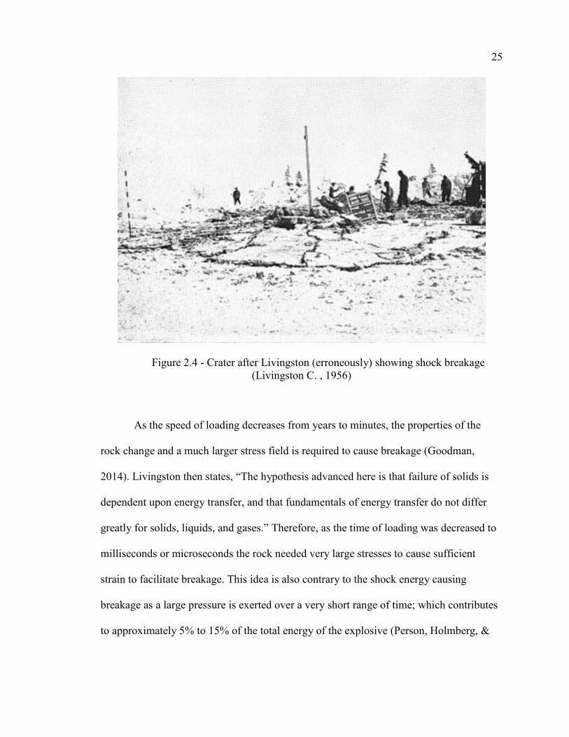
radial fractures and a conical shaped breakage around the borehole (Figure 2.4). As the
charge was brought closer to the surface the crater would break finer and material could
be ejected from the borehole. He believed that this showed that the shockwave had larger
effects than the gas pressure because the gas ejection of material occurred at a reduced
depth of burial and the shockwave showed effects at deeper burial.
However, Livingston never actually looked at the shock breakage or the energy
and time of these breakage planes. When reviewing pictures of the breakage observed in
Livingston’s crater studies it is now understood that this is not ‘shock breakage’ but

24
circular breakage around a borehole from lifting and bending of the upper layer of
material. For example, the author observed this same feature when blasting sandstone in
Saudi Arabia. In this situation, a large cave was present in the middle of the material to
be blasted and the mine loaded the material underneath the cave. When the explosive
detonated, the gas pressure filled this cave, causing lifting and bending of the surface.
This cave made the availability of the shockwave to rise to the surface impossible, yet the
same breakage patterns are observed. These features which were observed in
Livingston’s case are not because of the shockwave, but because as the explosive
detonated a large high-pressure gas is present in the borehole. If no free surface is present
and this gas is deep within the ground to where it is not of enough pressure to break out
and be released a large, high pressure gas sphere is formed. This causes the material
above the gas sphere to lift slightly causing bending of the material, which leads to this
circular breakage. This breakage is easily seen in the field by a large circular breakage
line at some distance from the borehole, following by fractures from the borehole to this
circular failure. This breakage pattern also has increased breakage around the borehole
where the material is lifted further, leading to increased strain. It was not the shockwave
that Livingston was observing but the effects of deeply confined charges.
Livingston also began the development of a new theory of failure of materials,
which was not based strain but on energy transfer. This energy transfer theory was not
only to look at the total magnitude of pressure or stress on an object but also the time that
this stress was applied (Livingston C. , 1956). For example, phenomena such as “creep”
and “relaxation,” which are slow moving deformation and strain of objects, which depend
on a large amount of time and lower stresses (Jeremic, 1994).
25
Figure 2.4 - Crater after Livingston (erroneously) showing shock breakage (Livingston C. , 1956)
As the speed of loading decreases from years to minutes, the properties of the
rock change and a much larger stress field is required to cause breakage (Goodman,
2014). Livingston then states, “The hypothesis advanced here is that failure of solids is
dependent upon energy transfer, and that fundamentals of energy transfer do not differ
greatly for solids, liquids, and gases.” Therefore, as the time of loading was decreased to
milliseconds or microseconds the rock needed very large stresses to cause sufficient
strain to facilitate breakage. This idea is also contrary to the shock energy causing
breakage as a large pressure is exerted over a very short range of time; which contributes
to approximately 5% to 15% of the total energy of the explosive (Person, Holmberg, &

26
Lee, 1994). Livingston’s two theories, the shock breakage of rock and energy transfer,
directly disputed each other.
However, at this time the Livingston crater theory was the new method, which
was quickly put into use through the Livingston crater theory equations. The base
Livingston crater theory used a strain-energy factor, which was dependent on the
explosive and material being blasted, to determine the maximum depth of burial that
breakage would be obtained. However, this widely varied and had to be determined
through experimentation for each rock type, structural region at a mine, and explosive
type. Case studies of this show that this was a complicated process, which resulted in
lengthy on-site studies and was entirely empirical based in application; relying minimally
or not at all on his base theoretical assumptions (Bauer, Harris, Lang, Preziosi, & Selleck,
1965).
2.3.2.2. U.S. Bureau of Mines Cratering Theory. Livingston’s research
acknowledged the fact that the gas pressure played an important role in the rock breakage
process, further facilitating breakage and leading to throw of material. However, others
took his new theory and began studying this new field of shockwave breakage. Perhaps
the most famous of this research was that of Duvall et. al. (Obert & Duvall, 1949; Obert
& Duvall, 1950; Duvall W. , 1953; Duvall & Atchison, 1957; Duvall & Petkof, 1959),
which was instantly spread and accepted, as these authors were part of the U.S. Bureau of
Mines researchers.
Basing their research off Livingston’s earlier work, crater formation was observed
from both holes vertically drilled into the rock mass and horizontal holes drilled into a
face with a bench off the side to observe directionality of breakage from the charge with

27
variations to the scale depth of burial of the charge. This carried on the same errors that
were present in the Livingston research, including the spherical charge assumptions and
misdiagnosis of breakage patterns.
Throughout nearly a decade of this research dozens of configurations of craters
was shot in various rock types. It was noted that in each case that when the depth of
burial was large enough that the gas could not break through and throw rock on the
surface, that breakage occurred near the surface. This was thought to be the shockwave
breaking along the surface after the effects of gas had been minimized, leading
researchers to believe that the shockwave was the primary breakage mechanism. This
theory was further propagated to assume that since the shockwave causes breakage at
deep burial, that when the burial is reduced to see gas effects, the shockwave had much
larger effects (Leet, 1960). In all reports of this time it was noted that the breakage from
this deep burial was minimal compared to actual breakage when the depth was reduced,
and the gas pressure could perform work on the rock. This was a confusing topic at the
time for many engineers and researchers not involved, as they believed the U.S. Bureau
of Mines but noted that in many situations topics such as stemming of a borehole, which
increased gas pressure but did not have any effect on the shockwave, were extremely
important for rock breakage (Johnsson & Hofmeister, 1961; Ash R. , 1963a; Ash R. ,
1963b).
2.3.2.3. Shockwave Spallation Theory. Concurrently with the Duvall and
Atchison work, Hino was working on the theoretical proof of the shock breakage theory.
At this time, high-speed photography was just being invented, which could capture these
breakage mechanisms.
28
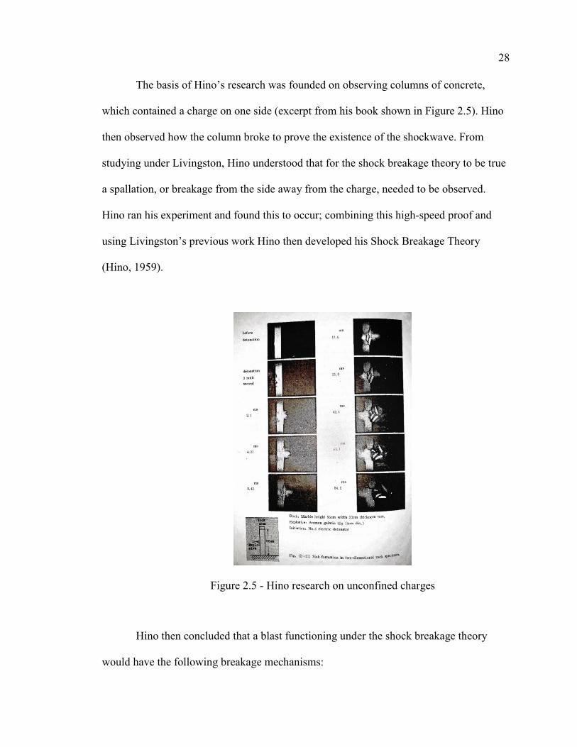
The basis of Hino’s research was founded on observing columns of concrete,
which contained a charge on one side (excerpt from his book shown in Figure 2.5). Hino
then observed how the column broke to prove the existence of the shockwave. From
studying under Livingston, Hino understood that for the shock breakage theory to be true
a spallation, or breakage from the side away from the charge, needed to be observed.
Hino ran his experiment and found this to occur; combining this high-speed proof and
using Livingston’s previous work Hino then developed his Shock Breakage Theory
(Hino, 1959).
Figure 2.5 - Hino research on unconfined charges
Hino then concluded that a blast functioning under the shock breakage theory
would have the following breakage mechanisms:

29
(1) The detonation of an explosive produces a crushed zone around it so far as the
intensity of shock wave produced by an explosive is greater than the
compressional strength of the rock
(2) Beyond the crushed zone there can be no breaking by compression due to
shock wave, however, the shock wave is reflected as a tension wave at a free
face. As the tensile strength of rock is much smaller than the compressional
one, rock can be broken by this tension wave, the range of breaking extending
from a free face inwards to the center of the charge.
(3) Only a part of the total energy of an explosive goes into shock wave and the
gases from detonation at high pressure expand doing additional work against
the resistant force of rock and against inertia of the big mass of rock
previously detached by shock wave from the ground. However, the contour of
the crater in time and space is primarily determined by shock wave.
This new theory overstated the shockwave from the explosive as the major
breakage mechanism in rock blasting and that the gases simply moved the broken rock
forward. This was radically different than previous schools of thought on rock breakage.
However, Hino had a few major problems with his experimental set-up and the
accompanying theory.
(1) The burden Hino used for his columns was approximately 15% of what is
used for that charge load in mine and quarry blasting. This error in improperly
scaling the charge to match the burden led to an overestimation of the
shockwave breakage mechanism. While this uncovered that the shockwave
was a breakage mechanism at a significantly reduced burden, it did not prove
30
that the shockwave was a major breakage mechanism at normal burdens in
field blasting.
(2) Hino’s research solely used unconfined explosive charges, where the pressure
from the gas is not withheld and was applied to the models. Therefore, it could
not be proven that the shock breakage was greater than the gas pressure.
Furthermore, with having to have a reduced burden to see the shock breakage
occur, it is likely that had this been a confined charge, the gas pressure would
have blown the model apart and across the room.
(3) In Hino’s proof of the shock breakage through compression around the
borehole (to generate the crushed zone) he takes into account attenuation of
the shockwave as it moves through the rock, assuming decay factors that are
favorable to the shock breakage argument. However, when Hino calculates the
maximum pressure from an explosive charge, he generates a detonation
pressure of 550,000 psi. Hino then uses the lowest compressional strength for
granite on record to show that this would be sufficient to break out to 4.76
charge diameters under compression.
(4) Hino is using the static compressive strength of granite, the dynamic
compressive strength of rock is typically much higher, where minimum
dynamic compressive strength of granite is around 58,000 psi (Qian, Qi, &
Wang, 2009; Livingston C. , 1956). This would change the crushed zone to a
maximum of 3 charge diameters for breakage under compression, which in
typical design accounts for less than 10% of the total burden.
31
(5) The crack speed of rock is 20% to 30% of the sonic velocity of the rock. If
crack tips are not stressed, they will not continue to grow. By the time the
cracks are one charge diameter away from the charge, the shock wave would
be 3 charge diameters away; causing no breakage to occur further out. This
would reduce the range that the shockwave could effectively break in
compression to less than one charge diameter due to the stress duration on the
crack tips.
(6) Hino also did not consider the attenuation of the shockwave as it moves
through a medium, losing energy both due to an increased volume it effects
and losses caused by friction (Cole, 1948). Using Hino’s graphs (Figure 4-1,
page 98) and the attenuation at a typical burden which is used in rock blasting
with commercial explosives, the shockwave would have a magnitude below
1000 psi when it reaches the free face. Further work has shown that the
attenuation of the shockwave in rock is much greater than Hino predicted and
would result in minimal shockwave pressure reaching the face (Spathis &
Wheatley, 2016).
(7) Hino updates the Livingston cratering theory with the shock breakage model
to develop design equations for a 90° conical crater. His powder factor for this
crater is 8 pounds per cubic yard; where traditional rock blasting would be
between 0.5 lbs/cyd and 2.0 lbs/cyd.
Later in his work Hino states that “only a part of the total energy available of
explosive goes into shock and a bigger part of it is consumed as work done by expansion
of gas.” At the end of his theory Hino states that a much larger portion of the energy goes
32
into gas than into the shock breakage; yet at the time he was trying to justify the
understanding of the day and developed a bias in his experimentation and further
analysis.
2.3.2.4. Strain Wave Theory. The work by Livingston, Duvall et. al., and Hino
was then developed into the Strain Wave Theory by Starfield (Starfield, 1966; Ben-Dor
& Takayama, 1992). This theory extended these principles and stated that crater
formation is solely based on the shock (strain) wave that is generated by the explosives
and that gas breakage is a minimal factor. This theory also introduced Hino’s work on
slabbing as the primary mechanism of rock breakage in this crater formation. This theory
was based on a series of theoretical craters that was physically tested, these craters are:
1. A gas crater which is formed through the effect solely of gas pressure
2. A strain crater which is formed through the effect solely of the strain wave
3. A combined crater which is formed from both the gas and strain crater
Starfield then theorized that if a strain wave crater could be fired without effects
of the gas crater, and this showed breakage at a depth deeper than the combined shock
and gas crater then it could be assumed that the strain wave was the primary breakage
mechanisms.
This was the same conclusion as the Duvall et. al. work, where the breakage was
mis-interpreted for studies ranging over a decade. Further authors later attempted to
expand the Strain Wave Theory including for application at weak seams and joints in the
rock mass. The Strain Wave Theory was widely refuted through its existence for inability
to match field conditions and improper theoretical development. Large grant funding
went into proving the theory; however, it was never successfully proven.

33
2.3.2.5. Refutation of the application of shockwaves in blasting. These
theories and research were heavily disputed based on several inconsistencies, including
the inability to use with ANFO explosives (Ash R. , 1974), the inability to have a true
shockwave nature even in high shockwave producing explosives (Cook M. A., 1974), and
the inability to apply theory to real, practical blasting scenarios (Langefors & Kihlstrom,
1973).
The existence of the shockwave was not disputed, and further researched went
into the understanding of how the shockwave affects the rock breakage process. Through
a series of testing it was determined that the shock wave had a total of between 5% to
15% of the total energy of the blast (Persson, Lundborg, & Johansson, 1970). Model and
full-scaled studies showed that breakage of the face in blasting did not occur from
shockwave spallation in blasting but instead the first face movement occurred at five to
ten times longer than it would take the shockwave to reach the free face (Persson,
Ladegaard-Pedersen, & Kihlstrom, 1969; Noren, 1956). Further studies showed that for a
typical borehole to experience shockwave spallation on the face, the borehole would have
to be loaded to 8 lbs/cyd (5kg/m3) or higher depending on the rock type, over eight times
the typical explosive load in rock blasting (Lang & Favreau, 1974; Persson, Lundborg, &
Johansson, 1970). Typical loads for bench blasting are around 1lbs/cyd (0.6 kg/m3).
Researchers have utilized high speed photography with physical models to
compare the effects of shock breakage with powder factors near 8 lbs/cyd (5kg/m3).
Figures 2.6 through 2.10 contain previously unpublished photographs taken by Dr. Calvin
J. Konya that show one of the time sequences of the physical models. These models are
cubic blocks of plexiglass with a ruler put behind them to determine scale. When a
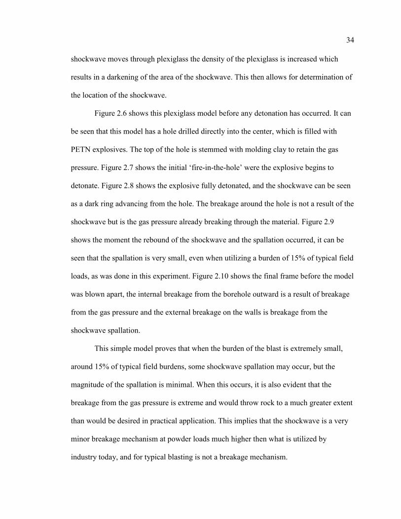
34
shockwave moves through plexiglass the density of the plexiglass is increased which
results in a darkening of the area of the shockwave. This then allows for determination of
the location of the shockwave.
Figure 2.6 shows this plexiglass model before any detonation has occurred. It can
be seen that this model has a hole drilled directly into the center, which is filled with
PETN explosives. The top of the hole is stemmed with molding clay to retain the gas
pressure. Figure 2.7 shows the initial ‘fire-in-the-hole’ were the explosive begins to
detonate. Figure 2.8 shows the explosive fully detonated, and the shockwave can be seen
as a dark ring advancing from the hole. The breakage around the hole is not a result of the
shockwave but is the gas pressure already breaking through the material. Figure 2.9
shows the moment the rebound of the shockwave and the spallation occurred, it can be
seen that the spallation is very small, even when utilizing a burden of 15% of typical field
loads, as was done in this experiment. Figure 2.10 shows the final frame before the model
was blown apart, the internal breakage from the borehole outward is a result of breakage
from the gas pressure and the external breakage on the walls is breakage from the
shockwave spallation.
This simple model proves that when the burden of the blast is extremely small,
around 15% of typical field burdens, some shockwave spallation may occur, but the
magnitude of the spallation is minimal. When this occurs, it is also evident that the
breakage from the gas pressure is extreme and would throw rock to a much greater extent
than would be desired in practical application. This implies that the shockwave is a very
minor breakage mechanism at powder loads much higher then what is utilized by
industry today, and for typical blasting is not a breakage mechanism.
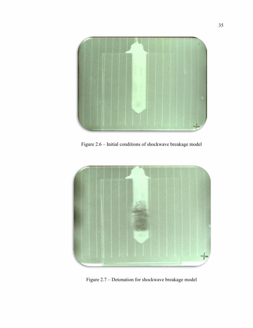
35
Figure 2.6 – Initial conditions of shockwave breakage model
Figure 2.7 – Detonation for shockwave breakage model
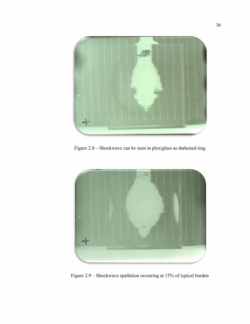
36
Figure 2.8 – Shockwave can be seen in plexiglass as darkened ring
Figure 2.9 – Shockwave spallation occurring at 15% of typical burden
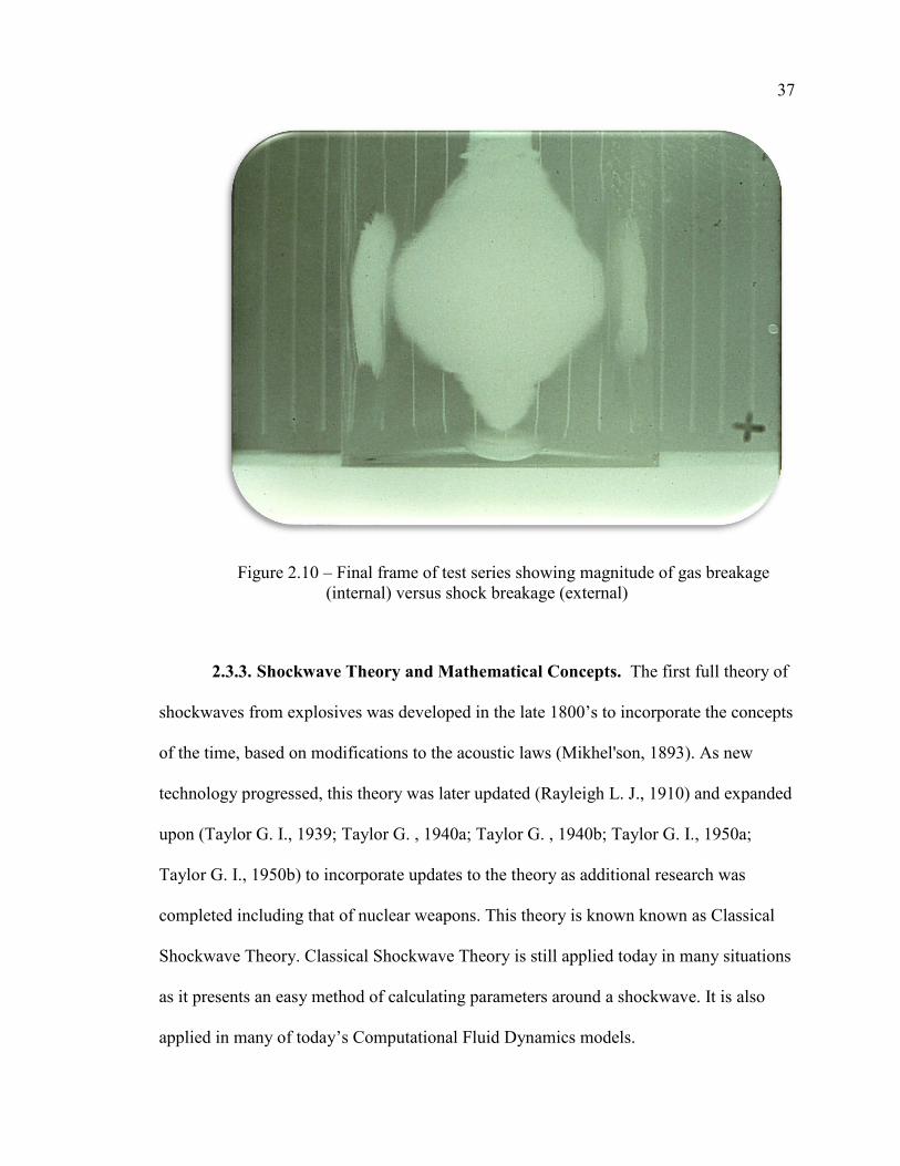
37
Figure 2.10 – Final frame of test series showing magnitude of gas breakage (internal) versus shock breakage (external)
2.3.3. Shockwave Theory and Mathematical Concepts. The first full theory of
shockwaves from explosives was developed in the late 1800’s to incorporate the concepts
of the time, based on modifications to the acoustic laws (Mikhel'son, 1893). As new
technology progressed, this theory was later updated (Rayleigh L. J., 1910) and expanded
upon (Taylor G. I., 1939; Taylor G. , 1940a; Taylor G. , 1940b; Taylor G. I., 1950a;
Taylor G. I., 1950b) to incorporate updates to the theory as additional research was
completed including that of nuclear weapons. This theory is known known as Classical
Shockwave Theory. Classical Shockwave Theory is still applied today in many situations
as it presents an easy method of calculating parameters around a shockwave. It is also
applied in many of today’s Computational Fluid Dynamics models.
38
Classical Shockwave theory has been greatly expanded to incorporate numerous
mathematical models for various materials and conditions. Modern shockwave theory has
been thoroughly explained in other texts (Cooper, 1996; Zel'dovich & Raizer, 2002) and
is beyond the purview of this dissertation. Instead this dissertation will focus on
explaining the basic concepts of shockwaves and introducing the mathematical formula
which will be used later in this discussion.
A shockwave is a wave which has a very rapid rise in pressure causing a
compression in a material. This shockwave is followed by a decay of the wave, which is
often discussed as a rarefaction wave. This shockwave can be formed in many ways
including impacts, supersonic events, or detonations of explosives. The event causing the
shockwave will determine how the shockwave is developed and the original and final
form. Regardless of the formation, a shockwave is a wave that has a very large pressure
and due to the large pressure travels faster than the speed of sound in the material.
Acoustical approximations can begin to be used to develop the principals behind a
shock wave. The basis of this would then rely on a term known as Impedance (Z), which
is presented in Equation 3.
𝑍𝑍 = 𝜌𝜌𝑉𝑉𝑠𝑠 (3)
where Z is the impedance of a rock in kilograms per square meter seconds, ρ is the
density in kilograms per cubic meter, and Vs is the sonic velocity of the material in
meters per second.
When a shockwave is travelling through one medium and hits a boundary
between that medium and another, part of the shockwave is transmitted into the second
medium and part of the shockwave is reflected back into the original medium traveling in

39
the opposite direction. For example, if a right moving shockwave in air hits a granite
ledge, part of the shockwave will be transmitted into the granite as a right moving
shockwave and part of the shockwave will be reflected in the air as a left-moving
shockwave. The intensity of the shockwave which is transmitted or reflected can be
calculated using equations 4 and 5, respectively (Worsey P. , 2016).
𝐼𝐼𝑡𝑡 = 4𝑍𝑍1𝑍𝑍2(𝑍𝑍1+𝑍𝑍2)2 (4)
𝐼𝐼𝑟𝑟 = (𝑍𝑍1− 𝑍𝑍2)2
(𝑍𝑍1+ 𝑍𝑍2)2 (5)
where It is the intensity of the shockwave transmitted, Ir is the intensity of the shockwave
reflected, Z1 is the impedance of the originating material, and Z2 is the impedance of the
receiving material.
The following discussion will focus only on those waves which are planar and
interaction boundaries which are at a 90° angle. Furthermore, it will be assumed that at
no point will a medium be defined as being thinner than the wavelength of the
shockwave.
The pressure of the detonation wave can be estimated using the Chapman-Jouguet
(CJ) pressure equation. While more advanced models have been given to determine the
pressure to a more exact level, for explosives with a specific gravity of 1.0 to 1.8 a
simplified equation has been proposed (Cooper, 1996) and will be used to estimate the
detonation shockwave pressure for various explosives. This equation is:
𝑃𝑃𝐶𝐶𝐶𝐶 = 𝜌𝜌𝐷𝐷2
4 (6)

40
where PCJ is the Chapman-Jouguet shockwave detonation pressure in GPA, ρ is the
density of the explosive in grams per cubic centimeter, and D is the velocity of detonation
in meters per second.
2.4. GAS PRESSURIZATION BREAKAGE IN COMMERCIAL BLASTING
Combustion, (fire), has been one of the fundamental principles that drove
humanity out of the dark ages and to the top of the food chain (Harari, 2011). Aristotle
and Heraclitus of Ephesus viewed combustion as the universal force of creation and these
philosophers, along with humankind, pondered the phenomena of combustion (Jaffe,
1930). Originally it was believed that combustion was a special element that was found
within materials, and it wasn’t until the 1600s that scientific theory was applied to the
thought of combustion. Fire was eliminated as an element and instead the Theory of
Phlogiston was developed (Becher, 1667). The phlogiston theory stated that all material
had a component, called phlogiston, which was released when the item was burned, as
burning wood and other materials caused a loss in mass. This theory had many challenges
brought on early, including that some compounds such as metals gained mass when
burned, yet the theory was defended.
The concept of phlogiston and the misunderstanding of combustions and
generation of gases led to researchers incorrectly attempting to quantify the force of
propellants and explosives. The first published mention of the force of gunpowder stated
that the force produced from gunpowder was due to increased elasticity in the air between
grains of black powder, which was caused by heating as the gunpowder burned (Hire,
41
1702). At this time, it was believed that the pressure of gunpowder was approximately 75
psi.
As understandings of combustion and gas generation advanced, new theories of
the force of gunpowder emerged. The first concept of gunpowder forming gases was
developed in 1743 (Robbins, 1743) where it was believed that black powder, when
combusted, would turn into gas which would take up 236 times the original volume of the
charge. It was then assumed with increases in temperature of these gases a pressure of
15,000 psi could be achieved in the bore of a gun. New research later showed that
gunpowder could reach up to 30,000 psi (Hutton, 1778). The first direct measurements of
the pressure associated with gunpowder were made using very small charges, typically
under one gram, to fire projectiles of varying weights. With this experimentation it was
determined that gunpowder could have a pressure of upwards of 426,182 psi with
theoretical calculations of 1,485,600 psi (Count of Rumford, 1797).
Theoretical and model testing of gunpowder continued with numerous authors
making claims for the final products of the combustion and the pressures associated with
gunpowder in the bores of guns. However, the majority of the work that can still be
considered today to hold accuracy was completed by Sir Andrew Nobel in the late 1800s
defining both the products of the combustion (Nobel & Abel, 1875) and the associated
pressures (Nobel S. A., 1892). This testing concluded that in testing of artillery with
Pebble Powder, Cannon Grade Black Powder, the pressure from 12 pounds of propellant
was 31,800 psi, which is approximately 2,650 psi per pound or 6 psi per gram of black
powder. A reproduction of Sir Andrew Nobel’s graph is shown in Figure 2.11, which
shows the pressure profile of black powder.
42
Work completed by Otuonye then advanced the understanding of pressure profiles
of explosives, but this time the borehole dynamics and effects of pressure on stemming
material was studied (Otuonye, 1981). This is the only research which has attempted to
quantify the pressure inside of a borehole from a decoupled charge. The pressure profiles
of the borehole filled with a decoupled charge of high explosives has many similarities to
that of Nobel’s work; with the main difference being the magnitude of the pressure. The
high explosive produced much greater pressures than the low explosive. This research
does not consider the shockwave, only the gas pressure in the device affecting these
pressures. This shows that high explosives, due to a combination of the gases, rate of
combustions, the temperature of combustion, and gas volume produced lead to an
increase in borehole pressure. Figure 2.12 shows a reproduction of Otuonye’s work and
Table 2.1 has some of the results obtained by Otuonye for peak pressure based on charge
weight. Otuonye’s work is the only measurement of borehole pressures for a decoupled
hole and will be relied upon for this work as no other data exists.
At this time, it had been shown that the variation of density of the explosive will
affect the velocity of detonation and the total pressure developed in the bore. It was also
understood at this time that depending on the speed of combustion the pressure profile
could rapidly change, even when the same theoretical gas volume was produced in a
certain diameter bore (Berthelot, 1892).
This work was proven theoretically and experimentally, and Table 2.2 is a
reproduction of the table produced by Nobel showing pressure in both closed vessels and
in a gun with variations in density and propellant type (Nobel S. A., 1892).

43
Figu
re 2
.11
Pres
sure
in th
e bo
re o
f a c
anno
n fro
m v
ario
us p
rope
llant
s afte
r Nob
el (N
obel
S. A
., 18
92)
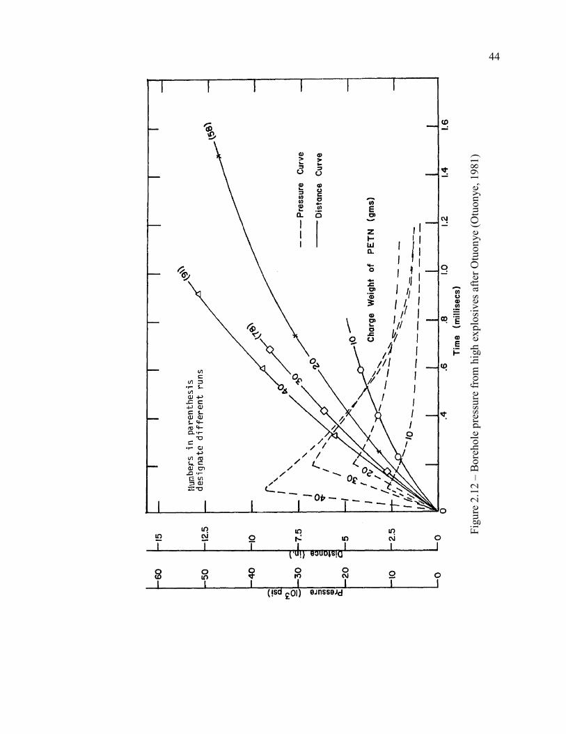
44
Figu
re 2
.12
– Bo
reho
le p
ress
ure
from
hig
h ex
plos
ives
afte
r Otu
onye
(Otu
onye
, 198
1)

45
The theory for the actual pressure of the gas produced by explosives was also
expanded from a theoretical standpoint. Another theory was that the differences in
pressure between explosive types was the result of the different gaseous products that
were formed from the explosives, which would change the total pressure due to the
intermolecular forces (Quinan, 1912). This early work was known as dissociation and
looked at the type of molecule developed in the detonation process and the effects of the
high-density effects of the explosive gases. Sarran’s Theory also added further to the
development of gas pressure from an explosive charge by introducing the heat of the
explosion (Sarran, 1884). While the magnitude of the heat of detonation was dramatically
overemphasized in Sarran’s work, it did give the explosive industry another tool to
incorporate into explosive gas pressure models.
Low density gases can be accurately modeled using the ideal gas law, however for
high-density gases, new equations of state needed to be developed. This is due, in part, to
the fact that when a gas is at high pressure and high densities the co-volume of the gas
begins to become a substantial part of the total volume. At extreme pressures the
molecules are in contact or nearly in contact with one another and the pressure is then
mainly due to the contact forces between molecules (Johansson & Persson, 1970).
2.4.1. Becker-Kistiakowsky-Wilson (BKW) Equation of State. Becker
developed an early equation of state for the detonation gases, assuming that the co-
volume was an exponential (Becker, 1922b; Becker, 1922a). His equation is:
𝑃𝑃𝑒𝑒 = 𝜌𝜌𝜌𝜌𝜌𝜌𝑇𝑇𝑒𝑒[1 + 𝑏𝑏𝜌𝜌𝑒𝑒𝑏𝑏𝜌𝜌 − 𝛼𝛼𝜌𝜌2 + 𝛽𝛽𝜌𝜌7] (7)
Where Pe is the explosive pressure, ρ is density, n is number of moles, R is the universal
gas constant, Te is the temperature of detonation, and b is co-volume.
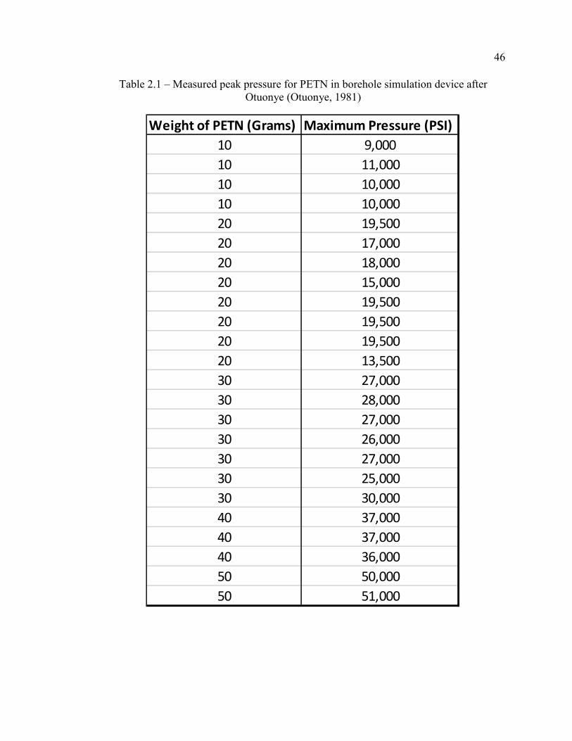
46
Table 2.1 – Measured peak pressure for PETN in borehole simulation device after Otuonye (Otuonye, 1981)
Weight of PETN (Grams) Maximum Pressure (PSI)10 9,00010 11,00010 10,00010 10,00020 19,50020 17,00020 18,00020 15,00020 19,50020 19,50020 19,50020 13,50030 27,00030 28,00030 27,00030 26,00030 27,00030 25,00030 30,00040 37,00040 37,00040 36,00050 50,00050 51,000
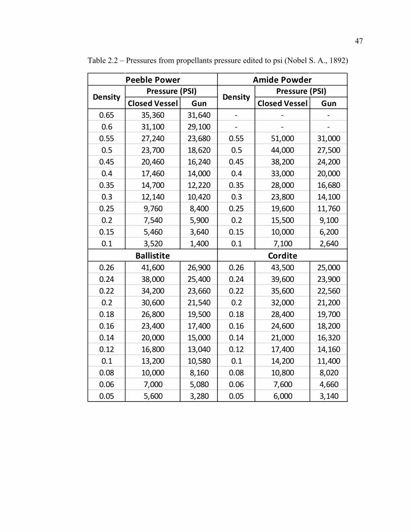
47
Table 2.2 – Pressures from propellants pressure edited to psi (Nobel S. A., 1892)
Closed Vessel Gun Closed Vessel Gun0.65 35,360 31,640 - - -0.6 31,100 29,100 - - -
0.55 27,240 23,680 0.55 51,000 31,0000.5 23,700 18,620 0.5 44,000 27,500
0.45 20,460 16,240 0.45 38,200 24,2000.4 17,460 14,000 0.4 33,000 20,000
0.35 14,700 12,220 0.35 28,000 16,6800.3 12,140 10,420 0.3 23,800 14,100
0.25 9,760 8,400 0.25 19,600 11,7600.2 7,540 5,900 0.2 15,500 9,100
0.15 5,460 3,640 0.15 10,000 6,2000.1 3,520 1,400 0.1 7,100 2,640
0.26 41,600 26,900 0.26 43,500 25,0000.24 38,000 25,400 0.24 39,600 23,9000.22 34,200 23,660 0.22 35,600 22,5600.2 30,600 21,540 0.2 32,000 21,200
0.18 26,800 19,500 0.18 28,400 19,7000.16 23,400 17,400 0.16 24,600 18,2000.14 20,000 15,000 0.14 21,000 16,3200.12 16,800 13,040 0.12 17,400 14,1600.1 13,200 10,580 0.1 14,200 11,400
0.08 10,000 8,160 0.08 10,800 8,0200.06 7,000 5,080 0.06 7,600 4,6600.05 5,600 3,280 0.05 6,000 3,140
Peeble Power Amide Powder
DensityPressure (PSI)
DensityPressure (PSI)
Ballistite Cordite
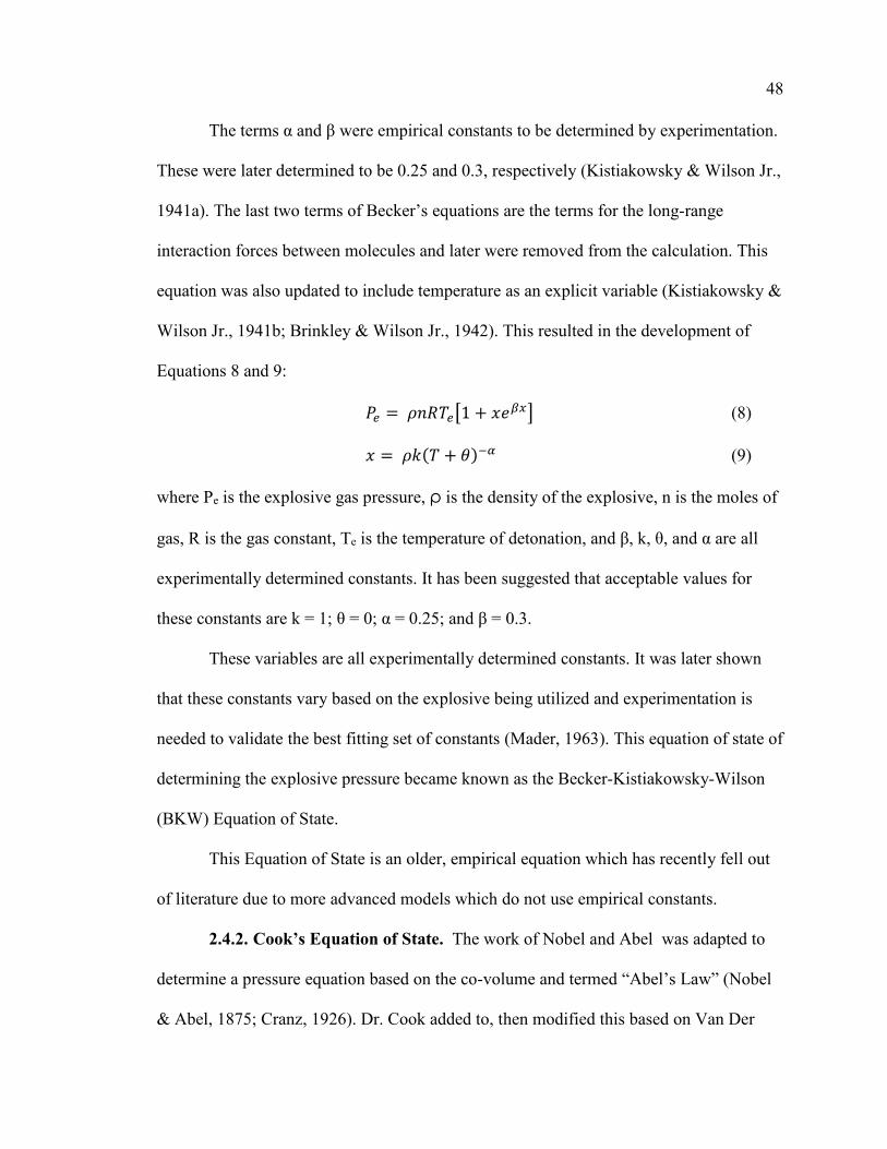
48
The terms α and β were empirical constants to be determined by experimentation.
These were later determined to be 0.25 and 0.3, respectively (Kistiakowsky & Wilson Jr.,
1941a). The last two terms of Becker’s equations are the terms for the long-range
interaction forces between molecules and later were removed from the calculation. This
equation was also updated to include temperature as an explicit variable (Kistiakowsky &
Wilson Jr., 1941b; Brinkley & Wilson Jr., 1942). This resulted in the development of
Equations 8 and 9:
𝑃𝑃𝑒𝑒 = 𝜌𝜌𝜌𝜌𝜌𝜌𝑇𝑇𝑒𝑒�1 + 𝑥𝑥𝑒𝑒𝛽𝛽𝛽𝛽� (8)
𝑥𝑥 = 𝜌𝜌𝜌𝜌(𝑇𝑇 + 𝜃𝜃)−𝛼𝛼 (9)
where Pe is the explosive gas pressure, ρ is the density of the explosive, n is the moles of
gas, R is the gas constant, Te is the temperature of detonation, and β, k, θ, and α are all
experimentally determined constants. It has been suggested that acceptable values for
these constants are k = 1; θ = 0; α = 0.25; and β = 0.3.
These variables are all experimentally determined constants. It was later shown
that these constants vary based on the explosive being utilized and experimentation is
needed to validate the best fitting set of constants (Mader, 1963). This equation of state of
determining the explosive pressure became known as the Becker-Kistiakowsky-Wilson
(BKW) Equation of State.
This Equation of State is an older, empirical equation which has recently fell out
of literature due to more advanced models which do not use empirical constants.
2.4.2. Cook’s Equation of State. The work of Nobel and Abel was adapted to
determine a pressure equation based on the co-volume and termed “Abel’s Law” (Nobel
& Abel, 1875; Cranz, 1926). Dr. Cook added to, then modified this based on Van Der
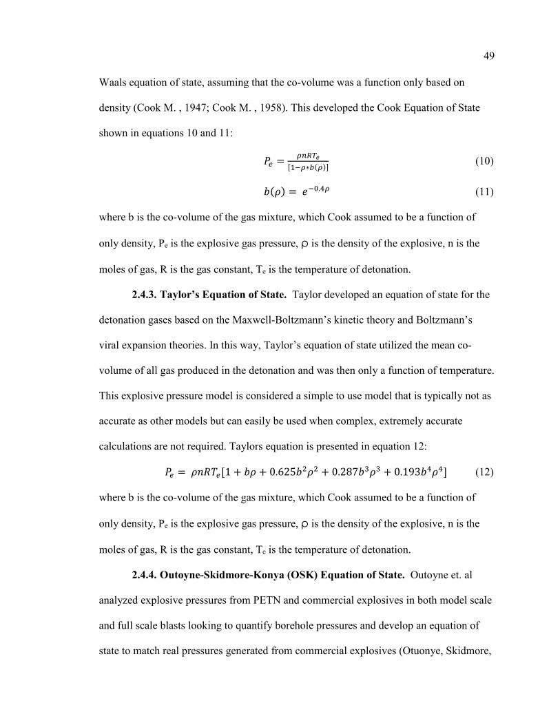
49
Waals equation of state, assuming that the co-volume was a function only based on
density (Cook M. , 1947; Cook M. , 1958). This developed the Cook Equation of State
shown in equations 10 and 11:
𝑃𝑃𝑒𝑒 = 𝜌𝜌𝜌𝜌𝜌𝜌𝑇𝑇𝑒𝑒[1−𝜌𝜌∗𝑏𝑏(𝜌𝜌)] (10)
𝑏𝑏(𝜌𝜌) = 𝑒𝑒−0.4𝜌𝜌 (11)
where b is the co-volume of the gas mixture, which Cook assumed to be a function of
only density, Pe is the explosive gas pressure, ρ is the density of the explosive, n is the
moles of gas, R is the gas constant, Te is the temperature of detonation.
2.4.3. Taylor’s Equation of State. Taylor developed an equation of state for the
detonation gases based on the Maxwell-Boltzmann’s kinetic theory and Boltzmann’s
viral expansion theories. In this way, Taylor’s equation of state utilized the mean co-
volume of all gas produced in the detonation and was then only a function of temperature.
This explosive pressure model is considered a simple to use model that is typically not as
accurate as other models but can easily be used when complex, extremely accurate
calculations are not required. Taylors equation is presented in equation 12:
𝑃𝑃𝑒𝑒 = 𝜌𝜌𝜌𝜌𝜌𝜌𝑇𝑇𝑒𝑒[1 + 𝑏𝑏𝜌𝜌 + 0.625𝑏𝑏2𝜌𝜌2 + 0.287𝑏𝑏3𝜌𝜌3 + 0.193𝑏𝑏4𝜌𝜌4] (12)
where b is the co-volume of the gas mixture, which Cook assumed to be a function of
only density, Pe is the explosive gas pressure, ρ is the density of the explosive, n is the
moles of gas, R is the gas constant, Te is the temperature of detonation.
2.4.4. Outoyne-Skidmore-Konya (OSK) Equation of State. Outoyne et. al
analyzed explosive pressures from PETN and commercial explosives in both model scale
and full scale blasts looking to quantify borehole pressures and develop an equation of
state to match real pressures generated from commercial explosives (Otuonye, Skidmore,
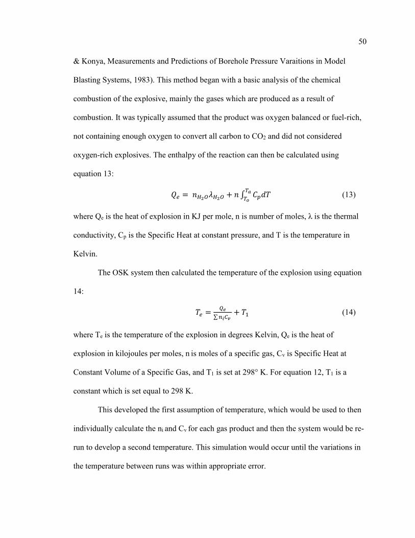
50
& Konya, Measurements and Predictions of Borehole Pressure Varaitions in Model
Blasting Systems, 1983). This method began with a basic analysis of the chemical
combustion of the explosive, mainly the gases which are produced as a result of
combustion. It was typically assumed that the product was oxygen balanced or fuel-rich,
not containing enough oxygen to convert all carbon to CO2 and did not considered
oxygen-rich explosives. The enthalpy of the reaction can then be calculated using
equation 13:
𝑄𝑄𝑒𝑒 = 𝜌𝜌𝐻𝐻2𝑂𝑂𝜆𝜆𝐻𝐻2𝑂𝑂 + 𝜌𝜌 ∫ 𝐶𝐶𝑝𝑝𝑑𝑑𝑇𝑇𝑇𝑇𝑎𝑎𝑇𝑇𝑜𝑜
(13)
where Qe is the heat of explosion in KJ per mole, n is number of moles, λ is the thermal
conductivity, Cp is the Specific Heat at constant pressure, and T is the temperature in
Kelvin.
The OSK system then calculated the temperature of the explosion using equation
14:
𝑇𝑇𝑒𝑒 = 𝑄𝑄𝑒𝑒∑𝜌𝜌𝑖𝑖𝐶𝐶𝑣𝑣
+ 𝑇𝑇1 (14)
where Te is the temperature of the explosion in degrees Kelvin, Qe is the heat of
explosion in kilojoules per moles, n is moles of a specific gas, Cv is Specific Heat at
Constant Volume of a Specific Gas, and T1 is set at 298° K. For equation 12, T1 is a
constant which is set equal to 298 K.
This developed the first assumption of temperature, which would be used to then
individually calculate the ni and Cv for each gas product and then the system would be re-
run to develop a second temperature. This simulation would occur until the variations in
the temperature between runs was within appropriate error.
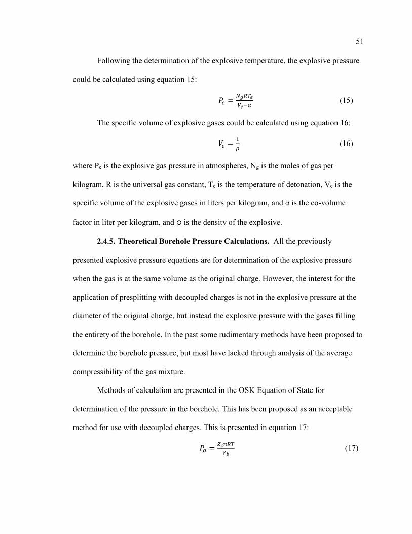
51
Following the determination of the explosive temperature, the explosive pressure
could be calculated using equation 15:
𝑃𝑃𝑒𝑒 = 𝑁𝑁𝑔𝑔𝜌𝜌𝑇𝑇𝑒𝑒𝑉𝑉𝑒𝑒−𝛼𝛼
(15)
The specific volume of explosive gases could be calculated using equation 16:
𝑉𝑉𝑒𝑒 = 1𝜌𝜌 (16)
where Pe is the explosive gas pressure in atmospheres, Ng is the moles of gas per
kilogram, R is the universal gas constant, Te is the temperature of detonation, Ve is the
specific volume of the explosive gases in liters per kilogram, and α is the co-volume
factor in liter per kilogram, and ρ is the density of the explosive.
2.4.5. Theoretical Borehole Pressure Calculations. All the previously
presented explosive pressure equations are for determination of the explosive pressure
when the gas is at the same volume as the original charge. However, the interest for the
application of presplitting with decoupled charges is not in the explosive pressure at the
diameter of the original charge, but instead the explosive pressure with the gases filling
the entirety of the borehole. In the past some rudimentary methods have been proposed to
determine the borehole pressure, but most have lacked through analysis of the average
compressibility of the gas mixture.
Methods of calculation are presented in the OSK Equation of State for
determination of the pressure in the borehole. This has been proposed as an acceptable
method for use with decoupled charges. This is presented in equation 17:
𝑃𝑃𝑔𝑔 = 𝑍𝑍𝑐𝑐𝜌𝜌𝜌𝜌𝑇𝑇𝑉𝑉𝑏𝑏
(17)
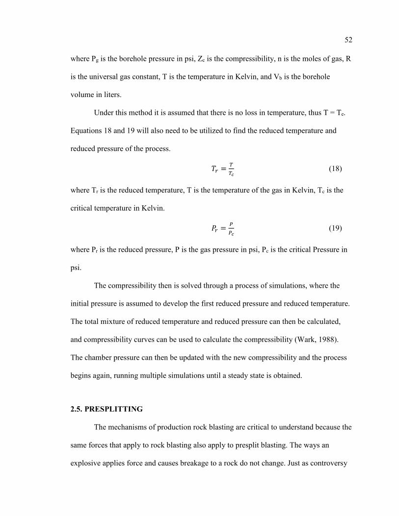
52
where Pg is the borehole pressure in psi, Zc is the compressibility, n is the moles of gas, R
is the universal gas constant, T is the temperature in Kelvin, and Vb is the borehole
volume in liters.
Under this method it is assumed that there is no loss in temperature, thus T = Te.
Equations 18 and 19 will also need to be utilized to find the reduced temperature and
reduced pressure of the process.
𝑇𝑇𝑟𝑟 = 𝑇𝑇𝑇𝑇𝑐𝑐
(18)
where Tr is the reduced temperature, T is the temperature of the gas in Kelvin, Tc is the
critical temperature in Kelvin.
𝑃𝑃𝑟𝑟 = 𝑃𝑃𝑃𝑃𝑐𝑐
(19)
where Pr is the reduced pressure, P is the gas pressure in psi, Pc is the critical Pressure in
psi.
The compressibility then is solved through a process of simulations, where the
initial pressure is assumed to develop the first reduced pressure and reduced temperature.
The total mixture of reduced temperature and reduced pressure can then be calculated,
and compressibility curves can be used to calculate the compressibility (Wark, 1988).
The chamber pressure can then be updated with the new compressibility and the process
begins again, running multiple simulations until a steady state is obtained.
2.5. PRESPLITTING
The mechanisms of production rock blasting are critical to understand because the
same forces that apply to rock blasting also apply to presplit blasting. The ways an
explosive applies force and causes breakage to a rock do not change. Just as controversy
53
existed in the mechanisms of a production blast, the theories behind a presplit mechanism
have not been well defined and relatively few studies have been completed on presplit
formation. In today’s blasting industry both shock breakage (Zhang, 2016) and gas
pressurization of the borehole (Konya & Konya, 2017a) is presented in modern technical
papers as mechanisms of presplitting. Many have also argued that the mechanism behind
the presplit is unimportant or academic, which may be true for the traditional case of
presplitting, which remains the same under almost all circumstances. However, with the
advent of Precision Presplitting the mechanism behind a presplit is of importance, as
changes to dimensions such as the spacing of boreholes and explosive load in a hole are
designed to meet the structural geology and rock properties. Without an understanding of
the mechanisms behind a presplit formation, a strategic design to eliminate overbreak
while allowing for smooth breakage is impossible.
The first large scale explosive presplit was produced on the Niagara Power
Project, which was completed in 1962 (Paine, Holmes, & Clark, 1961; Paine, Holmes, &
Clark, 1962). This project was based in dolomite and limestone with a single layer of
shale near the bottom of the excavation. It was required to have smooth walls to pour
concrete against. During the project, numerous methods of controlled blasting were
attempted including line drilling, line drilling with explosive loads in every third hole,
modified cushion blasting, decks of dynamites throughout the borehole, and finally
presplitting. It was reported that the only method that produced satisfactory results to
minimize overbreak was the presplitting, which was accomplished by taping 1 ¼” by 4”
sticks of dynamite on Primacord every 12 inches. The boreholes were 2 ½” to 3” in
diameter, spaced 24 inches apart and stemmed with crushed gravel. This resulted in an
54
increased rock excavation rate and a reduction in scaling by a factor of 10. Additionally,
the project had significant savings on concrete costs and increased safety as the walls
were cleaned smooth (Paine, Holmes, & Clark, 1961). Following the project presplitting
was widely accepted as the best and most cost-effective method of overbreak control.
Based on this work, researchers of presplitting both in a laboratory and in a
practical setting began looking into the decoupling of charges, or the reduction of the
diameter of the explosive compared to the diameter of the borehole. This was done to
decrease the dynamic gas flow on the borehole wall and to reduce the gas pressure in the
borehole (Konya, Britton, & Lukovic, 1987) preventing large compressive strengths
which would lead to overbreak (Day, 1982). However, this increase in decoupling ratio
also led to minimal shock pressure transmission into the rock mass due to large
impedance mismatches between explosives and air, then air and rock.
With the large increase in research of shock breakage in rock blasting, many
authors began to investigate possible effects of shockwave collision between boreholes to
develop tensile zones and causing presplit formation (DuPont, 1975; Crosby & Bauer,
1982). This theory was widespread due to the popularity of the DuPont Blasters
Handbook, and it is still circulated amongst many leading organizations today
(International Society of Explosive Engineers, 2016) and researchers (Salmi &
Hosseinzadch, 2014). This theory was heavily disputed and shown in numerous studies of
the day and it was shown that no correlation exists between the dynamic shockwave and
the presplit formation, with numerous studies showing that the quasi-static gas pressure
in the borehole was responsible for presplit formation (Konya C. , 1973; Worsey P. ,
1981; Worsey, Farmer, & Matheson, 1981; Daehnke, Rossmanith, & Kouzniak, 1996).

55
Additional studies were conducted utilizing a propellant charge, Pyrodex, to fire a
presplit blast. These propellant charges produce no shockwave, as they deflagrate, not
detonate (Akhavan, 2011), which completely isolated the gas pressure as the only
working energy. Using the same principles as in traditional presplit design (Konya C. ,
1980), the propellant charges produced the exact same results as a presplit blast that was
fired with detonating explosives (Konya, Barret, & Smith, 1986). This proved that
presplit mechanisms on a full-scale blast had no reliance on the shockwave generated by
detonating explosives.
This led to the development of a Precision Presplit style of blasting, where
extremely light loads of detonating cord are utilized to prevent all breakage around the
borehole while forming the presplit fracture (Konya C. , 1982). This design utilized
closely spaced boreholes of 24 inches or less to minimize the impacts of rock structure on
the presplit (Worsey P. , 1984; Worsey & Qu, 1987; Tariq & Worsey, 1996). As this
design methodology has begun widespread use, new empirical research into the explosive
loading based on the rock properties has been developed (Konya & Konya, 2015; Konya
& Konya, 2017b; Konya & Konya, 2016).
This method of Precision Presplitting has effectively zero shock energy to form a
fracture after accounting for impedance mismatches (Cooper, 1996), non-ideal detonation
(Cook M. A., 1974), and attenuation of the shockwave in the rock mass (Spathis &
Wheatley, 2016). It has then been theorized that the mechanism behind the presplit
formation is due to large hoop stresses which are generated between the boreholes
causing a fracture, with no advancement of the fracture from gas penetration (Konya &
Konya, 2017a). The hoop stress field for a thick-walled pressure vessel has been one
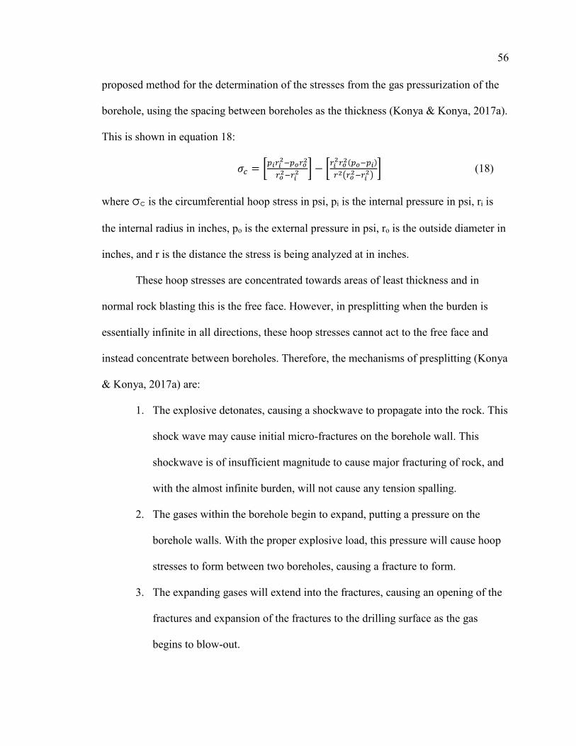
56
proposed method for the determination of the stresses from the gas pressurization of the
borehole, using the spacing between boreholes as the thickness (Konya & Konya, 2017a).
This is shown in equation 18:
𝜎𝜎𝑐𝑐 = �𝑝𝑝𝑖𝑖𝑟𝑟𝑖𝑖2−𝑝𝑝𝑜𝑜𝑟𝑟𝑜𝑜2
𝑟𝑟𝑜𝑜2−𝑟𝑟𝑖𝑖2 � − �𝑟𝑟𝑖𝑖
2𝑟𝑟𝑜𝑜2(𝑝𝑝𝑜𝑜−𝑝𝑝𝑖𝑖)𝑟𝑟2�𝑟𝑟𝑜𝑜2−𝑟𝑟𝑖𝑖
2�� (18)
where σc is the circumferential hoop stress in psi, pi is the internal pressure in psi, ri is
the internal radius in inches, po is the external pressure in psi, ro is the outside diameter in
inches, and r is the distance the stress is being analyzed at in inches.
These hoop stresses are concentrated towards areas of least thickness and in
normal rock blasting this is the free face. However, in presplitting when the burden is
essentially infinite in all directions, these hoop stresses cannot act to the free face and
instead concentrate between boreholes. Therefore, the mechanisms of presplitting (Konya
& Konya, 2017a) are:
1. The explosive detonates, causing a shockwave to propagate into the rock. This
shock wave may cause initial micro-fractures on the borehole wall. This
shockwave is of insufficient magnitude to cause major fracturing of rock, and
with the almost infinite burden, will not cause any tension spalling.
2. The gases within the borehole begin to expand, putting a pressure on the
borehole walls. With the proper explosive load, this pressure will cause hoop
stresses to form between two boreholes, causing a fracture to form.
3. The expanding gases will extend into the fractures, causing an opening of the
fractures and expansion of the fractures to the drilling surface as the gas
begins to blow-out.

57
4. If the proper amount of explosive and stemming is used, the explosive will
blow the stemming out of the borehole and the gas pressure will be released
through the top of the borehole (Choked Flow Gas Theory)
By analyzing the steps of a presplit, one can quickly begin to see the
importance of many variables including:
1. Explosive Load – this will directly influence the total gas pressure inside of the
borehole. The large gas pressure in the borehole can lead to overbreak around the
hole through various mechanisms, including:
a. A fractured zone due to too great a gas pressures (compressional
breakage) if no free face is available
b. Too large of a gas volume to easily flow through the borehole, leading to
failure at the crest (cratering) and enlargement of cracks
c. Too little of an explosive load can also be a problem, as insufficient gas
build-up will not form large enough hoop stresses to fracture from
borehole to borehole.
2. Stemming – If the stemming creates a stemming plug (Konya & Walter, 1990)
then the stemming will lock into the borehole. This will cause the highly
pressurized gases to:
a. Crater the borehole, causing backbreak at the top of the resulting face
b. Open and expand cracks, potentially causing additional breakage or
opening existing cracks, joints, or bedding planes.

58
c. If the stemming is insufficient to momentarily hold the gas pressure, the
pressure inside of the borehole will be of insufficient magnitude to form a
large hoop stress, resulting in no fracture between boreholes.
3. Spacing – if the spacing is too large, the hoop stresses will be insignificant to
cause the proper fracture to form resulting in a rough face. If the spacing is too
small, the hoop stresses will be so large that additional fracturing will occur
extending outward from radial cracks and multiple radial cracks will connect
between blastholes
2.5.1. Traditional Presplitting. Traditional Presplitting will be defined as a
method of presplit blasting which utilizes presplit powder, or other explosives, in which
the load in the borehole is, at minimum, 0.30 pounds per foot. The typical case of
traditional presplitting would be using a 7/8” presplit powder, which has a load per foot
of 0.3 lbs/ft of borehole length, a spacing of 36” (3 feet), and a stemming length of 30”
(2.5 ft). These presplits can have the charge weight expanded and/or the spacing
increased or decreased. The traditional presplitting techniques have not incorporated
geologic factors into the design criteria and instead rely on basic rules of thumb for the
design.
These rules of thumb are shown in Equations 21 and 22 (Konya & Walter, 1990):
𝐸𝐸𝐸𝐸 = 𝑑𝑑ℎ2
28 (21)
𝑆𝑆 = 10𝑑𝑑ℎ (22)
where EL is the explosive load in pounds per foot, S is the spacing in inches, and dh is the
diameter of the borehole in inches. The constant in the equation 22 can be modified and
typically falls between 8 and 14 but is set as 10 for the first test blasting in an area.
59
In the past, changes to the design of a traditional presplit were based on the split-
factor, which is the load per square area of face. A blaster may have a presplit that works
in a certain situation and attempt to increase the explosive load and modify the spacing.
The blaster would then compute how many pounds of explosive were being used to split
a certain square footage of wall. They would then assume that this split-factor would hold
for presplitting that rock type and change the spacing between boreholes based upon
changing explosive weight to fit the split factor. This improperly assumed that the
relationship was linear and was known to perform very poorly for design purposes,
except in rare cases. Recent work has shown that the function is not linear, and it has
been shown why split-factor was a poor method of design (Worsey P. , 1981; Konya &
Konya, 2017a).
2.5.2. Precision Presplitting. Precision Presplitting is a method of presplitting
which utilizes extremely light charge loads, along with the borehole spacing and rock
properties to develop a design which will cause a fracture to form without overbreak. The
spacing of the borehole will be a function of the desired control, the structural geology,
and the cost of blasting.
This method is commonly used in weak, or heavily jointed rock where normal
presplit blasting does not work. This method of presplitting uses the proper amount of
explosive load to cause a smooth fracture to form between boreholes, without causing
overbreak or excessive shattering of the wall.
In previous years, Precision Presplitting utilized 18” to 24” spacing and the
explosive load was determined through test blasts. These test blasts would be detonated,
and the back wall would be exposed. It then took an experienced engineer or blaster who

60
has worked extensively with presplitting to determine what explosive load was ‘optimal’
for the presplit. If the proper explosive load was not used in the test blast, in many cases
the blaster or engineer would say that the geology was not proper for presplitting. This
occurred in many cases when using the common presplit powders because of the
overloading of explosives. This method of Precision Presplitting has been used on
projects such as Highway 28 in Pennsylvania, Folsom Dam, Kentucky Locks, Panama
Canal, Grundy Virginia Remediation Project and many other large construction projects
and in mines worldwide and is the primary presplitting technique used by the Army Corp
of Engineers (U.S. Army Corp of Engineers, 2018).
In recent years, Anthony Konya and Dr. Calvin Konya have derived methods to
calculate the optimal explosive load for a precision presplit with a spacing of 24” (0.61m)
center to center based on the Young’s Modulus of the rock with tests shown in Figure
2.13. (Konya & Konya, 2016). The ‘typical’ method of Precision Presplitting utilizes 24”
(0.61m) of spacing with a 3” (75mm) diameter blasthole and 30” (0.75m) of stemming.
This simplifies design to having the rock type be the only consideration for the explosive
load.
This was then expanded upon to include equations to determine the explosive load
required to cause a fracture to form based on the rocks Young’s Modulus, the Konya
Presplit Factor, and the spacing between boreholes. The calculation of the Konya Presplit
Factor is shown in Equation 23:
𝐾𝐾 = �40579𝐸𝐸
�0.625
(23)
where K is the Konya Presplit Constant and E is the Young’s Modulus in GPa.
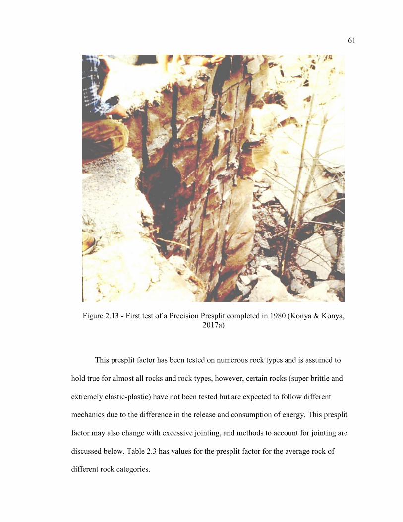
61
Figure 2.13 - First test of a Precision Presplit completed in 1980 (Konya & Konya, 2017a)
This presplit factor has been tested on numerous rock types and is assumed to
hold true for almost all rocks and rock types, however, certain rocks (super brittle and
extremely elastic-plastic) have not been tested but are expected to follow different
mechanics due to the difference in the release and consumption of energy. This presplit
factor may also change with excessive jointing, and methods to account for jointing are
discussed below. Table 2.3 has values for the presplit factor for the average rock of
different rock categories.

62
The next consideration in the design of the Precision Presplit is the spacing that
will be used between boreholes, center to center. This is of extreme importance, as even
properly varying the explosive load with the spacing will produce different fracturing.
This is because the rock is non-homogenous and has joints and fractures that will cause
fractures to deviate and stop fracture growth.
Furthermore, the increase in spacing results in an increased explosive load, which
can lead to over-pressurization of the borehole. This can result in additional breakage
around the borehole. The spacing must then be chosen for each site to provide the desired
wall characteristics based on the local geologic structures. This can also dramatically
increase the cost for overbreak control, as decreasing the spacing significantly increases
cost, especially in drilling and initiation.
The effects of the structural geology in a local area been studied in the past to
determine how presplits behave in non-homogenous rock. It is now understood that
jointing and other discontinuities between two boreholes of a presplit will cause increased
backbreak and a worse wall, and the joint frequency between boreholes will be one of the
major limiting factors of the maximum spacing.
In a study by Syed Tariq and Dr. Paul Worsey (Tariq & Worsey, 1996), the
effects of discontinuities on presplit spacing was analyzed. This work was completed for
a traditional presplit and it was concluded that:
1. Increased discontinuities can help facilitate a presplit, however, a worse
presplit facture is produced
2. A larger joint frequency between boreholes enhances the effects of cratering
of the borehole, a worse presplit fracture is produced
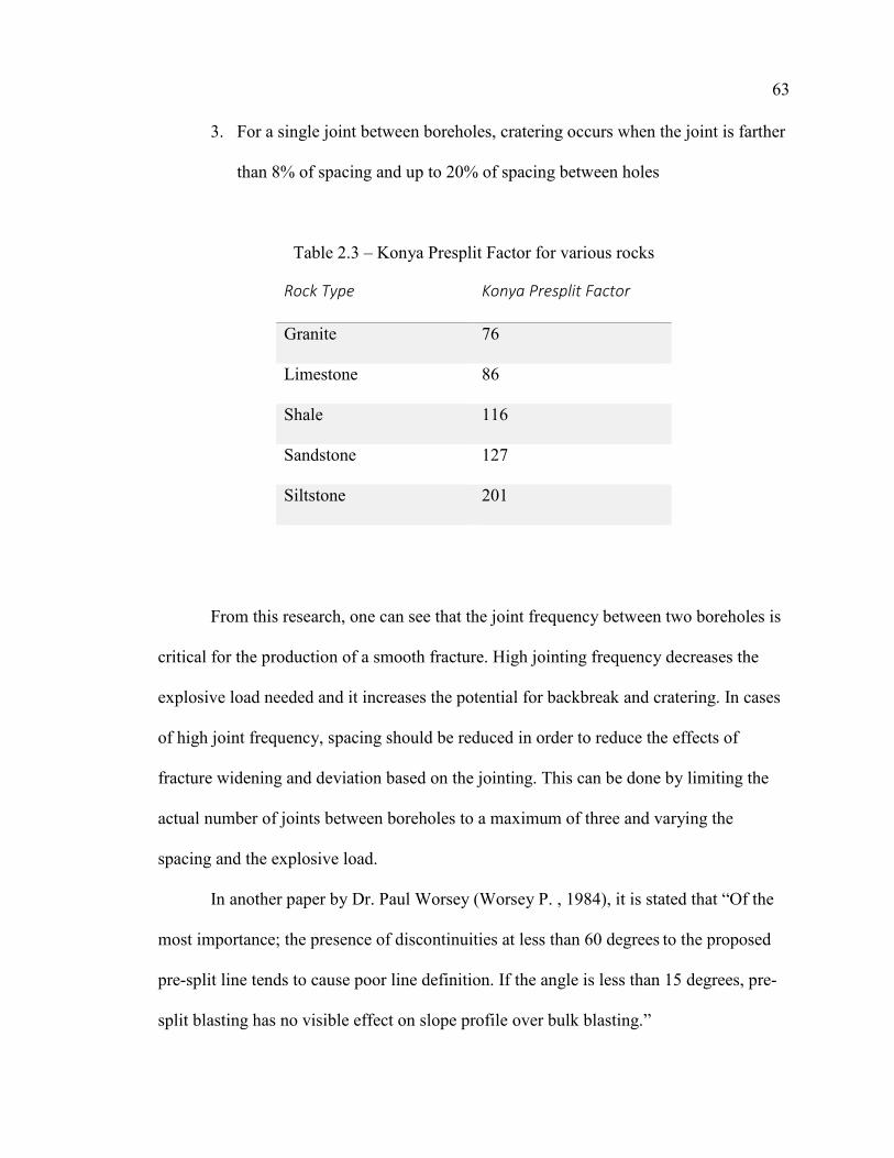
63
3. For a single joint between boreholes, cratering occurs when the joint is farther
than 8% of spacing and up to 20% of spacing between holes
Table 2.3 – Konya Presplit Factor for various rocks
Rock Type Konya Presplit Factor
Granite 76
Limestone 86
Shale 116
Sandstone 127
Siltstone 201
From this research, one can see that the joint frequency between two boreholes is
critical for the production of a smooth fracture. High jointing frequency decreases the
explosive load needed and it increases the potential for backbreak and cratering. In cases
of high joint frequency, spacing should be reduced in order to reduce the effects of
fracture widening and deviation based on the jointing. This can be done by limiting the
actual number of joints between boreholes to a maximum of three and varying the
spacing and the explosive load.
In another paper by Dr. Paul Worsey (Worsey P. , 1984), it is stated that “Of the
most importance; the presence of discontinuities at less than 60 degrees to the proposed
pre-split line tends to cause poor line definition. If the angle is less than 15 degrees, pre-
split blasting has no visible effect on slope profile over bulk blasting.”

64
Dr. Worsey also states that the pre-split fractures will intersect discontinuities at
approximately right angles. This demonstrates not only the importance of spacing, but
also the orientation of the presplit in relation to the natural jointing of the rock mass.
If a smooth presplit fracture must be obtained in extremely jointed rock, the
author has used a spacing of 12” (0.30m) to reduce the effects of the discontinuities. In
rocks that are extremely massive, with minimal jointing or other discontinuities, the
spacing of the pre-split can be expanded much further to decrease the cost and maintain
similar walls.
Increasing the spacing on a Precision Presplit can be done in rock with a low joint
frequency, however considerations must be taken towards final wall conditions and
distance to free burden. The presplit mechanism works because the distance between
holes (spacing) is very small. As the spacing increases and the explosive load is
increased. This can result in breakage to other production holes within the blast pattern,
along geologic seams, and at the crest of the borehole.
Spacing can be properly expanded and a similar fracture can be maintained, as
long as the spacing is within reasonable distance, the rock is competent, and the explosive
load and decoupling ratio are adjusted accordingly. This will also cause a benefit by
reducing the cost of presplitting which is beneficial to the mining industry, which is often
in competition with other miners.
Decoupling ratio is defined as the ratio of the diameter of the drillhole to the
diameter of the explosive charge. Decoupling is used to minimize the pressure on the
borehole walls and prevent the micro-fracturing on the boreholes wall from the shock
wave (Konya, Britton, & Lukovic, 1987). Decoupling charges will also decrease the
65
density of gas in a borehole and reduce the pressure exerted on the borehole walls. This
helps to maintain control of a presplit and is a common technique used for wall control.
The borehole pressure is inversely proportional to the square of the decoupling
ratio (Figure 2.14) (Konya, Britton, & Gozon, 1985). Choked Gas Mass Flow is
proportional to the discharge area of the borehole. For applications of presplitting, such
as Precision Presplitting, where the decoupling ratio is large, the borehole must be
momentarily confined to create the proper hoop stress and fracture. This momentary hold
should last approximately 8ms or slightly less and then blow out, quickly allowing the
release of pressure from the borehole to avoid overbreaking the rock. In order to do this,
the borehole is generally stemmed using a stemming plug, along with drill cuttings to a
depth of 10 to 12 times the borehole diameter. This will allow proper decoupling of the
borehole to prevent excessive breakage while allowing the gas pressure to quickly be
released.
With the ability to calculate the presplit factor of different rocks one can now
approach the design of a precision presplit with an engineering approach. The explosive
of choice for a Precision Presplit is detonating cord. This is because detonating cord
provides a consistent, controllable amount of energy throughout its length. Detonating
cord fires reliably at small diameters whereas other commercially available explosives
cannot be used in small diameters. Detonating cord is also easy to work with, with proper
techniques it is simple to load, and explosive load variations can be made throughout the
borehole to account for different rock types in a single blast (example in Figure 2.15).
The explosive load with detonating cord, is calculated in grains per foot where
7,000 grains is equivalent to one pound of explosive. Using the Konya Presplit Factor (K)
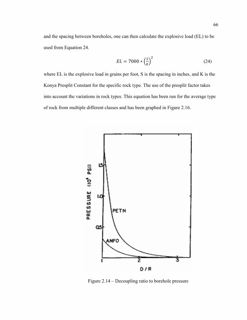
66
and the spacing between boreholes, one can then calculate the explosive load (EL) to be
used from Equation 24.
𝐸𝐸𝐸𝐸 = 7000 ∗ �𝑆𝑆𝐾𝐾�2 (24)
where EL is the explosive load in grains per foot, S is the spacing in inches, and K is the
Konya Presplit Constant for the specific rock type. The use of the presplit factor takes
into account the variations in rock types. This equation has been run for the average type
of rock from multiple different classes and has been graphed in Figure 2.16.
Figure 2.14 – Decoupling ratio to borehole pressure
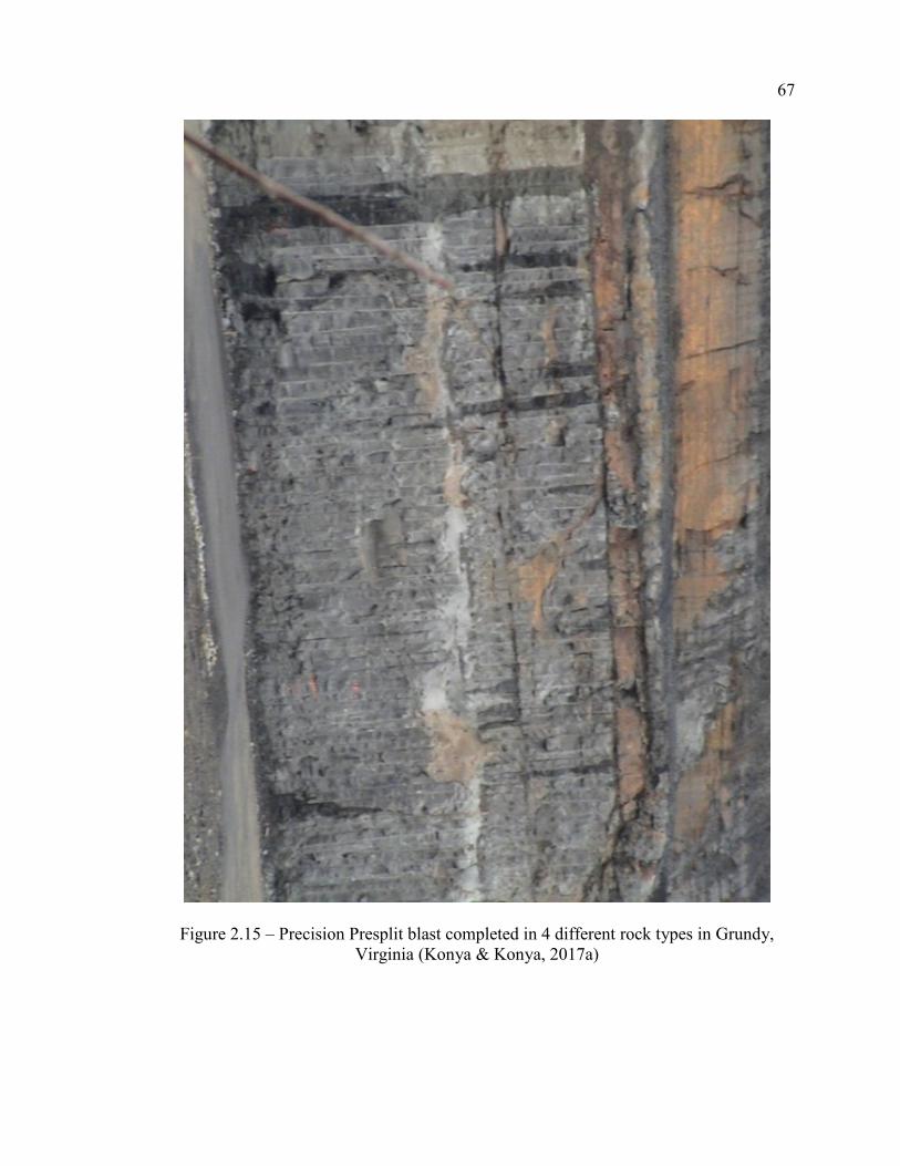
67
Figure 2.15 – Precision Presplit blast completed in 4 different rock types in Grundy, Virginia (Konya & Konya, 2017a)

68
Figu
re 2
.16
– Pr
ecis
ion
Pres
plit
load
var
iatio
ns b
ased
on
typi
cal v
alue
s for
spec
ific
rock
type

69
2.5.3. Propellant Presplitting. Propellant presplitting is a method of presplitting
which was tested to determine if propellants could be used to cause a presplit (Konya,
Barret, & Smith, 1986). This testing was completed to observe if the shockwave was an
important consideration for presplit blasting and was directly compared to presplits
completed with dynamite. These were full scale tests, which were completed in a granite
quarries in Georgia using a propellant known as Pyrodex. A comparison of Pyrodex to
Black Powder has been reproduced in Table 2.4. The results of various tests with the
dynamite versus the propellent have also been reproduced in Table 2.5.
The testing also utilized both loaded and unloaded holes with variations to the
hole diameter and the spacing of the holes. While the ‘split-factor’ was not used for
design on this project, it was used to compare the two explosives to determine the
economic feasibility of using the products. The split factors for the two explosives are
nearly identical and range between 0.04 to 0.07 pounds per square foot of new face
created. It was noted that once the borehole began to fracture, or in areas of weak rock,
the Pyrodex could not build up to pressure as confinement was lost.
It is important to note that the authors of this study reported and included several
pictures in the paper which show that the presplits performed the same between the
dynamite and the Pyrodex. In the situation of the Pyrodex no shockwave was produced
and the only force acting on the rock mass was that of the gas pressure. The formation of
a presplit from a propellant charge would not be possible under the currently proposed
theory of shockwave collisions. However, it is clearly evident that with no shockwave
being produced the presplit still fully formed. This states that the presplit is not a function
of the shockwave but of another mechanisms.
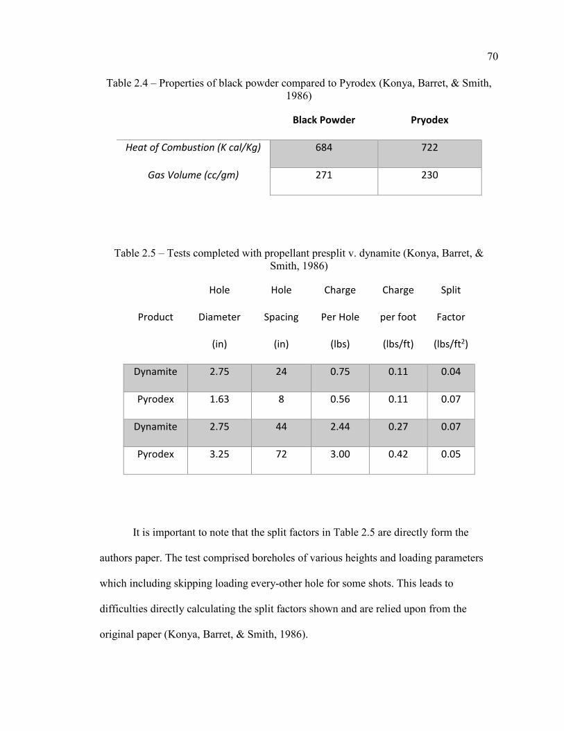
70
Table 2.4 – Properties of black powder compared to Pyrodex (Konya, Barret, & Smith, 1986)
Black Powder Pryodex
Heat of Combustion (K cal/Kg) 684 722
Gas Volume (cc/gm) 271 230
Table 2.5 – Tests completed with propellant presplit v. dynamite (Konya, Barret, & Smith, 1986)
Product
Hole
Diameter
(in)
Hole
Spacing
(in)
Charge
Per Hole
(lbs)
Charge
per foot
(lbs/ft)
Split
Factor
(lbs/ft2)
Dynamite 2.75 24 0.75 0.11 0.04
Pyrodex 1.63 8 0.56 0.11 0.07
Dynamite 2.75 44 2.44 0.27 0.07
Pyrodex 3.25 72 3.00 0.42 0.05
It is important to note that the split factors in Table 2.5 are directly form the
authors paper. The test comprised boreholes of various heights and loading parameters
which including skipping loading every-other hole for some shots. This leads to
difficulties directly calculating the split factors shown and are relied upon from the
original paper (Konya, Barret, & Smith, 1986).
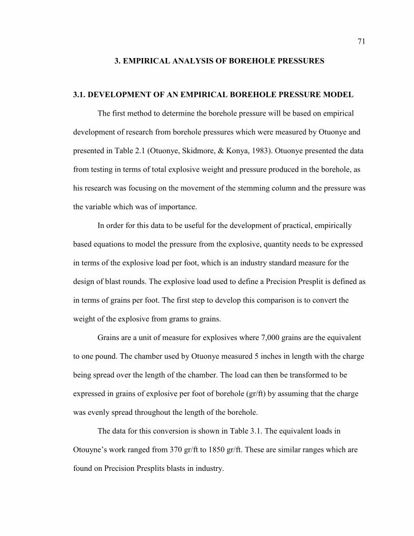
71
3. EMPIRICAL ANALYSIS OF BOREHOLE PRESSURES
3.1. DEVELOPMENT OF AN EMPIRICAL BOREHOLE PRESSURE MODEL
The first method to determine the borehole pressure will be based on empirical
development of research from borehole pressures which were measured by Otuonye and
presented in Table 2.1 (Otuonye, Skidmore, & Konya, 1983). Otuonye presented the data
from testing in terms of total explosive weight and pressure produced in the borehole, as
his research was focusing on the movement of the stemming column and the pressure was
the variable which was of importance.
In order for this data to be useful for the development of practical, empirically
based equations to model the pressure from the explosive, quantity needs to be expressed
in terms of the explosive load per foot, which is an industry standard measure for the
design of blast rounds. The explosive load used to define a Precision Presplit is defined as
in terms of grains per foot. The first step to develop this comparison is to convert the
weight of the explosive from grams to grains.
Grains are a unit of measure for explosives where 7,000 grains are the equivalent
to one pound. The chamber used by Otuonye measured 5 inches in length with the charge
being spread over the length of the chamber. The load can then be transformed to be
expressed in grains of explosive per foot of borehole (gr/ft) by assuming that the charge
was evenly spread throughout the length of the borehole.
The data for this conversion is shown in Table 3.1. The equivalent loads in
Otouyne’s work ranged from 370 gr/ft to 1850 gr/ft. These are similar ranges which are
found on Precision Presplits blasts in industry.

72
Table 3.1 – Borehole pressures (after Otuoyne) compared to charge weight per foot
Weight of Charge (Grams) Charge Weight per Foot (gr/ft)
Pressure (psi)
10 370 9,000 10 370 11,000 10 370 10,000 10 370 10,000 20 740 19,500 20 740 17,000 20 740 18,000 20 740 15,000 20 740 19,500 20 740 19,500 20 740 19,500 20 740 13,500 30 1110 27,000 30 1110 28,000 30 1110 27,000 30 1110 26,000 30 1110 27,000 30 1110 25,000 30 1110 30,000 40 1480 37,000 40 1480 37,000 40 1480 36,000 50 1850 50,000 50 1850 51,000
The data in Table 3.1 can then be plotted and a linear regression can be completed
to develop an empirical equation which relates the pressure to the explosive load in a
borehole. This results in Equation 25
𝑃𝑃𝑔𝑔 = 26.4𝐸𝐸𝐸𝐸 − 1372 (25)
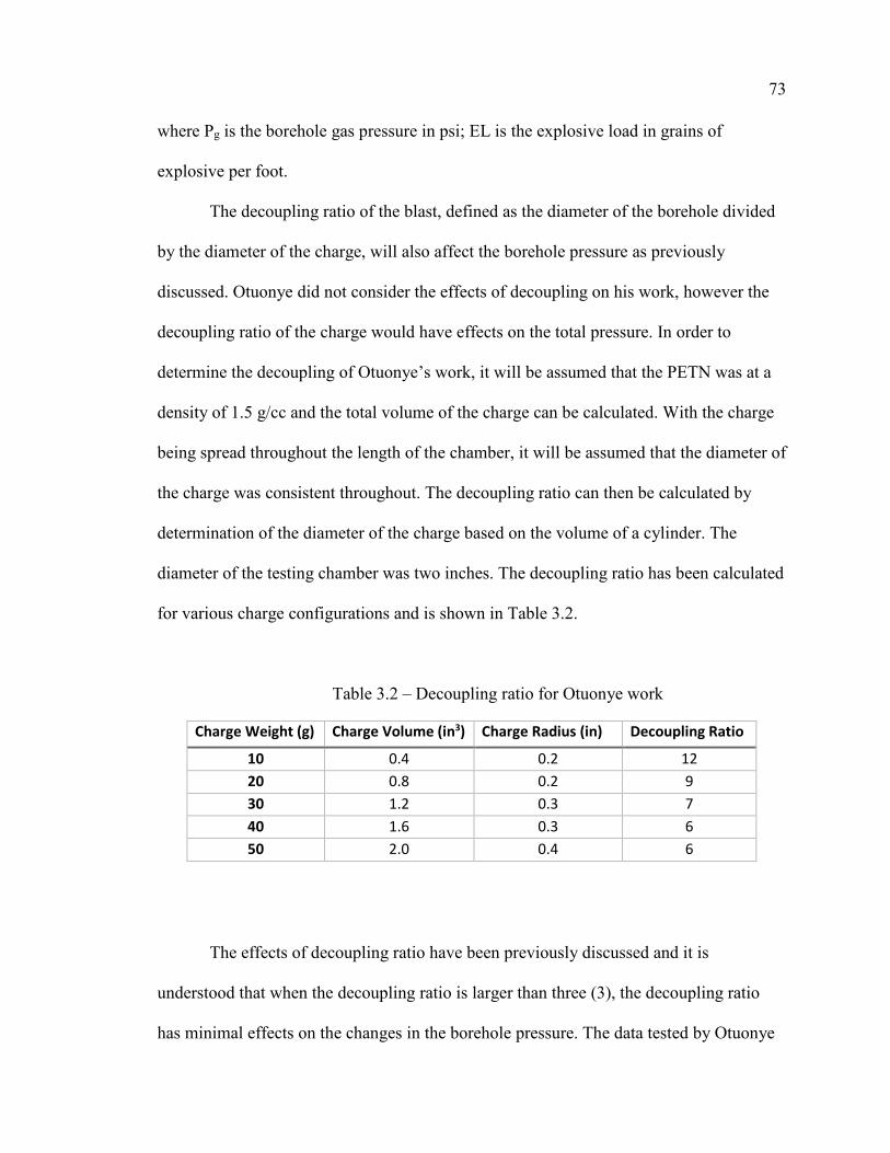
73
where Pg is the borehole gas pressure in psi; EL is the explosive load in grains of
explosive per foot.
The decoupling ratio of the blast, defined as the diameter of the borehole divided
by the diameter of the charge, will also affect the borehole pressure as previously
discussed. Otuonye did not consider the effects of decoupling on his work, however the
decoupling ratio of the charge would have effects on the total pressure. In order to
determine the decoupling of Otuonye’s work, it will be assumed that the PETN was at a
density of 1.5 g/cc and the total volume of the charge can be calculated. With the charge
being spread throughout the length of the chamber, it will be assumed that the diameter of
the charge was consistent throughout. The decoupling ratio can then be calculated by
determination of the diameter of the charge based on the volume of a cylinder. The
diameter of the testing chamber was two inches. The decoupling ratio has been calculated
for various charge configurations and is shown in Table 3.2.
Table 3.2 – Decoupling ratio for Otuonye work
Charge Weight (g) Charge Volume (in3) Charge Radius (in) Decoupling Ratio
10 0.4 0.2 12 20 0.8 0.2 9 30 1.2 0.3 7 40 1.6 0.3 6 50 2.0 0.4 6
The effects of decoupling ratio have been previously discussed and it is
understood that when the decoupling ratio is larger than three (3), the decoupling ratio
has minimal effects on the changes in the borehole pressure. The data tested by Otuonye

74
varied between a decoupling ratio of six (6) through twelve (12). For the purposes of this
dissertation, a decoupling ratio greater than three (3) will be considered a large
decoupling ratio which has no effect on borehole pressure. Therefore, Equation 23 can be
stated as being applicable to determine the borehole pressure for charges with a large
decoupling ratio for a borehole which is two inches in diameter.
Equation 23 is graphed along with Otuonye’s data in Figure 3.1 and is
seen to have a R2 value of 0.97, which implies an excellent fit of the data to be
modeled by the developed equation. A close inspection of the data does show that
there are some minor deviations at all the charge loads which can be considered
some experimental error. Figure 3.1 shows a linear relationship between the
borehole pressure and the explosive load. This proves that the previously made
assumption about large decoupling ratios is correct and no effects of reducing the
decoupling are realized within this range.
Furthermore, Otuonye’s work was completed with PETN which is the
same explosive that is used in Precision Presplitting. Different explosives will
detonate with variations in temperature and gas products, which will lead to
different borehole pressures. Equation 25 can only be used when the explosive
being utilized is PETN.
This introduces the base form of the Empirical Model which can be used
for estimating pressures in a borehole with a two-inch diameter. However, it is
important to develop methods for changing this borehole diameter

75
Figu
re 3
.1 –
Exp
losi
ve lo
ad to
bor
ehol
e pr
essu
re fo
r lar
ge d
ecou
plin
g in
a tw
o-in
ch d
iam
eter
hol
e (E
quat
ion
25)
76
3.2. MODIFICATION OF THE EMPIRICAL MODEL
Equation 23 has been shown to be applicable for the determination of the
borehole pressure under large decoupling for a two-inch diameter borehole. In order to
develop an equation that can accurately model the borehole pressure to be used in field
loading conditions, a model will have to be developed which can calculate the borehole
pressure with changing borehole diameter. The borehole pressure will have large changes
based on the borehole diameter due to the accompanying volume changes. The gas
volume generated by the explosive will have to occupy a larger space causing a reduction
in the pressure. For example, a three-inch hole has a volume which is 229% of the
volume of a two-inch hole. The detonation process and pressurization of a borehole is
extremely rapid and is treated as an adiabatic process which has no change in
temperature. Boyle’s law is an accepted technique for analyzing variations of pressure
with changes volume at a constant temperature and is shown in Equation 26.
𝑃𝑃1𝑉𝑉1 = 𝑃𝑃2𝑉𝑉2 (26)
where P1 is the original pressure, V1 is the original volume, P2 is the final pressure, and
V2 is the final temperature.
The original pressure would be that of the pressure in a two-inch diameter
borehole, which is presented in Equation 25. The original volume will be the volume of a
two-inch diameter borehole and the final volume will be the volume of the actual
borehole. The volume of the borehole can be calculated based on the volume of a
cylinder, which has been shown in Equation 27 in a modified form to include units
typical in the blasting industry.
𝑉𝑉𝑏𝑏 = 𝜋𝜋4𝑑𝑑ℎ2𝑃𝑃𝐶𝐶 (27)
77
where Vb is the volume of the borehole in cubic inches, dh is the diameter of the borehole,
and PC is the length of the powder column in inches. It is important to note that by using
the length of the powder column, it is assumed that the borehole will reach maximum
pressure before the stemming begins movement. This has been verified to be a true
assumption as maximum borehole pressure is not dependent on stemming movement or
the loss of stemming (Otuonye, 1981). Rearranging Equation 26 to isolate the final
pressure gives Equation 28
𝑃𝑃1𝑉𝑉1𝑉𝑉2
= 𝑃𝑃2 (28)
Substituting Equation 25 for P1 and Equation 25 for V1 and V2 gives Equation 29.
�(26.4𝐸𝐸𝐸𝐸−1372)∗�𝜋𝜋4∗22∗𝑃𝑃𝐶𝐶��
𝜋𝜋4𝑑𝑑ℎ
2𝑃𝑃𝐶𝐶= 𝑃𝑃2 (29)
where EL is the explosive load in grains per foot, PC is the length of powder column in
inches, dh is the diameter of the borehole in inches, and P2 is the borehole pressure in psi.
Simplification of Equation 29 gives Equation 30, which is the Empirical Model
for determination of the borehole pressure.
𝑃𝑃𝑔𝑔 = 105.6𝐸𝐸𝐸𝐸−5488𝑑𝑑ℎ2 (30)
where Pg is the borehole pressure in psi, EL is the explosive load in grains per foot, and
dh is the diameter of the borehole. The error for this equation is 5% to 10% from
measured values obtained by Otuonye, with an average of 8.8%.
Equation 30 can then be used to determine the borehole pressure based on the
changes in the explosive load and borehole diameter, assuming the decoupling ratio is
large, and the explosive is PETN. Equation 28 has been used to generate Figure 3.2
which shows changes in the borehole pressure based on changes to borehole diameter and

78
explosive load. The range of explosive load has been taken as 100 grains per foot to 1000
grains per foot, which is the explosive load typically found in Precision Presplitting.
Figure 3.2 shows, similar to Figure 3.1, that when the borehole diameter is set the
borehole pressure varies linearly with the explosive load.
Figure 3.3 shows the effects of a changing borehole diameter while maintaining a
constant explosive load. The three explosives loads shown here are commonly used in the
field for various rock types with a 24” spacing between boreholes, such as Shale (300
grains per foot), Limestone (500 grains per foot), and Granite (700 grains per foot).
Figure 3.3 shows that the effects of the explosive load to borehole pressure are large at a
borehole diameter under six inches, but when the borehole diameter exceeds six inches it
is difficult to generate substantial borehole pressures from Precision Presplitting, which
would be equivalent to a decoupling ratio of approximately 25. It would therefore be
advised that the decoupling ratio remain below 25 on any presplit blast from a borehole
pressure analysis.
Equation 30 is termed the Empirical Borehole Pressure Model which can be used
to quickly determine the borehole pressure from a charge with large decoupling (greater
than three) and a PETN based explosive. The benefit of this model is that it contains a
low error and is a simple and straightforward calculations. This model cannot take into
account different mixtures of detonation products, different densities of PETN, different
temperatures of detonation, or different methods of combustion (i.e. detonation versus
deflagration). Following sections of this dissertation will address these other topics from
a theoretical standpoint for more advanced modelling.

79
Figu
re 3
.2 –
Bor
ehol
e pr
essu
re v
aria
tions
of e
xplo
sive
load
with
con
stan
t bor
ehol
e di
amet
er
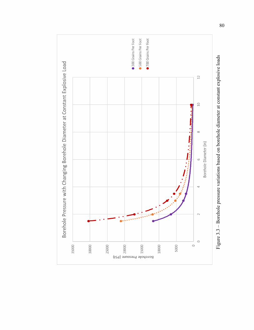
80
Figu
re 3
.3 –
Bor
ehol
e pr
essu
re v
aria
tions
bas
ed o
n bo
reho
le d
iam
eter
at c
onst
ant e
xplo
sive
load
s

81
3.3. EMPIRICAL MODEL FOR TYPICAL PRECISION PRESPLIT
The previously presented equations can be used to determine the variations in the
borehole pressure with variations to explosive load and borehole diameter. This was
needed in order to be able to determine the explosive load from a standard Precision
Presplit, which in a majority of situations will use a three-inch diameter borehole.
Substituting in three inches for the borehole diameter and simplifying Equation 30 gives
Equation 31 as a simplified borehole pressure equation for Precision Presplitting.
𝑃𝑃𝑔𝑔 = 11.7𝐸𝐸𝐸𝐸 − 610 (31)
where Pg is the borehole pressure in psi and EL is the explosive load in grains per foot.
This empirical equation allows for easy calculation of the borehole pressure based
on the explosive load and will be applied later in this dissertation for the determination of
the stress in the rock mass. This equation assumes that the borehole diameter is three-
inches, the decoupling ratio is greater than three, and the explosive used is PETN. Table
3.3 shows the calculation of the borehole pressure from variations to explosive load from
Equation 29.
Table 3.3 – Boreholes pressures for Precision Presplitting based on explosive load
Explosive Load (gr/ft)
Borehole Pressure (psi)
200 1730 300 2900 400 4070 500 5240 600 6410 700 7580

82
4. THEORETICAL ANALYSIS OF BOREHOLE PRESSURES
4.1. INTRODUCTION TO THEORETICAL MODELS
The empirical model presented in Equation 28 and 29 can be reliably used to
determine the detonation pressure of a PETN based explosive charge in boreholes of
varying diameter for a decoupling ratio above three. However, it would be beneficial to
develop a model which could be used to determine borehole pressures for variations in
explosive type and for decoupling ratios below three. This would give equations which
could be used to determine the borehole pressure for any situation in which explosives
are used to break rock. Without relevant empirical data for all scenarios, a theoretical
model can be developed which would be derived from accepted theories in chemistry,
thermodynamics, and hydrodynamics. The model would then be validated using the data
from Otuonye.
Two models are presented in this dissertation as theoretical models for the
determination of borehole pressure. The first model is derived from the detonation gas
pressure of the explosive, relying on the equations of state previously discussed. This
model can be considered a simplified model which has relatively little computational
time. The first model presented would likely still only be valid for a decoupling ratio
above three as it does not take into account compressibility of the gas at high pressures
and temperatures; however, it is applicable to any type of high explosive. The second
model is a more advanced model that relies on an iterative process. The second model is
assumed to be a more accurate model as it accounts for items such as the compressibility
of gases and could be used for low and high explosives at any decoupling ratio.
83
4.1.1. Temperature of Detonation. The first step in the use of either of these
models will be to determine the temperature of the explosion or combustion. The
determination of the temperature of the detonation can be done either through
experimental testing or through equations previously presented (Otuonye, Skidmore, &
Konya, 1983).
The measurements of a single crystal of unconfined PETN observe a temperature
of detonation of 4140 ± 70 K (Yoo, Holmes, Souers, Wu, & Ree, 2000). The
measurement of this detonation temperature is from a single crystal placed in an
unconfined state using a nanosecond time-resolved spectropyrometric system. However,
this data does not necessarily represent a comparison for the use of large amounts of
PETN in a borehole.
Explosives typically have a rating of run-up distance, which is the distance away
from the initiation point that the velocity of detonation reaches steady-state. This is
different from a deflagration-to-detonation transition which is the point at which the
explosive begins to detonate. PETN has a very short deflagration-to-detonation transition
and is typically assumed to detonate immediately upon initiation.
An explosive is not at full energy until it reaches the proper run-up distance and
the velocity of detonation is at the steady-state speed, even if it is detonating. The run-up
distance for PETN has been shown to vary from 1mm to 10mm, or larger depending on
the density and confinement of the charge (Reaugh, Curtis, & Maheswaran, 2017). It can
then be assumed that until this run-up point is reached the pressure and temperature of the
explosive will also not be at the maximum values. This implies that the temperature of
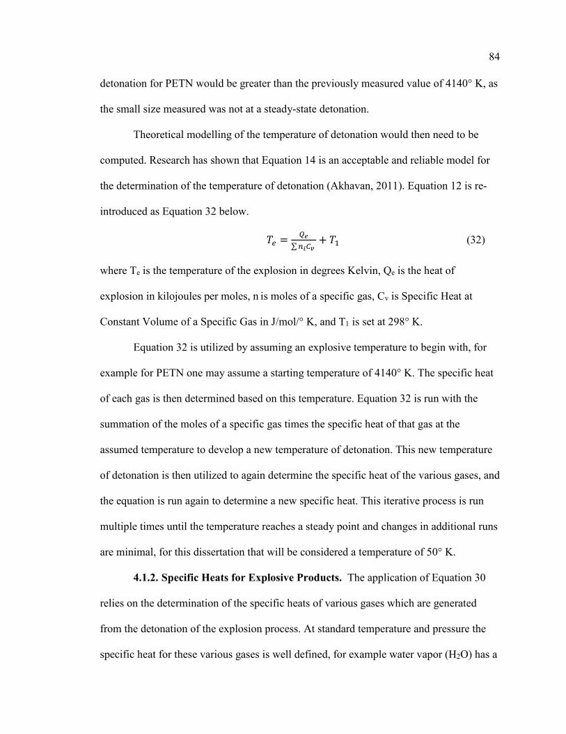
84
detonation for PETN would be greater than the previously measured value of 4140° K, as
the small size measured was not at a steady-state detonation.
Theoretical modelling of the temperature of detonation would then need to be
computed. Research has shown that Equation 14 is an acceptable and reliable model for
the determination of the temperature of detonation (Akhavan, 2011). Equation 12 is re-
introduced as Equation 32 below.
𝑇𝑇𝑒𝑒 = 𝑄𝑄𝑒𝑒∑𝜌𝜌𝑖𝑖𝐶𝐶𝑣𝑣
+ 𝑇𝑇1 (32)
where Te is the temperature of the explosion in degrees Kelvin, Qe is the heat of
explosion in kilojoules per moles, n is moles of a specific gas, Cv is Specific Heat at
Constant Volume of a Specific Gas in J/mol/° K, and T1 is set at 298° K.
Equation 32 is utilized by assuming an explosive temperature to begin with, for
example for PETN one may assume a starting temperature of 4140° K. The specific heat
of each gas is then determined based on this temperature. Equation 32 is run with the
summation of the moles of a specific gas times the specific heat of that gas at the
assumed temperature to develop a new temperature of detonation. This new temperature
of detonation is then utilized to again determine the specific heat of the various gases, and
the equation is run again to determine a new specific heat. This iterative process is run
multiple times until the temperature reaches a steady point and changes in additional runs
are minimal, for this dissertation that will be considered a temperature of 50° K.
4.1.2. Specific Heats for Explosive Products. The application of Equation 30
relies on the determination of the specific heats of various gases which are generated
from the detonation of the explosion process. At standard temperature and pressure the
specific heat for these various gases is well defined, for example water vapor (H2O) has a
85
specific heat of 1.996 KJ/kg/° K. This implies that to raise the temperature of steam one-
degree Kelvin, 1.996 KJ of energy need to be applied per kilogram of steam. At
temperatures below 1000° K the specific heat of gases minimally varies and as such
many basic thermodynamic texts and solutions assume a constant specific heat for a
certain gas. The major variations of specific heat below 1000° K comes from phase
changes (Smith, Van Ness, & Abbot, 2005).
However, when the temperature is raised significantly above 1000° K the specific
heat of substances begins to increase rapidly (Akhavan, 2011), for example at a
temperature of 2500° K the specific heat of water vapor is 2.987 KJ/kg/° K. The large
increase in the specific heat must be accounted for when determining the temperature of
the explosion due to the extremely high temperatures that are observed in a detonation.
This must be found for each of the products that will be produced in the detonation, as
each separate product has its own unique heat capacity. Currently minimal methods exist
for the determination of the specific heats for the various products encountered, as such
the author has developed equations based on a collection of data to determine the specific
heats based on variations in temperature.
4.1.2.1. Dulong-Petit Limit. Specific heats at high temperatures for solids are
typically determined based on the Dulong-Petit Law (Petit & Dulong, 1819) which states
that the specific heat of a solid will vary between 22.5 J/mol/° K and 30 J/mol/° K with a
value of 25 J/mol/° K as the standard constant. This was proven to apply as a maximum
limit for the specific heat based on the temperature of the process for elemental solids
(Einstein, 1906). Recent research has shown that solid compounds can exceed this limit
value.

86
However, at a certain temperature, which varies based on the solid compound, the
compound will reach a maximum heat capacity at which the heat capacity will stop
increasing for any further increase in temperature. This maximum heat capacity is known
as the Dulong-Petit Limit. K2S, which is a solid compound produced by black powder,
has a specific heat capacity which reaches a Dulong-Petit Limit of 70.226 J/mol/° K at a
temperature of 1000° K.
4.1.2.2. PETN detonation products. The formula for the detonation of PETN
can be found below. Using a simplified detonation product approach, the gases which are
formed are Nitrogen, Steam, Carbon Dioxide, and Carbon Monoxide. This will be used to
determine which products will need to have specific heat equations developed for use in
Equation 32. The heat of combustion is shown in Table 4.1.
PETN Combustion: 𝐶𝐶5𝐻𝐻8𝑁𝑁4𝑂𝑂12 → 2𝑁𝑁2 + 4𝐻𝐻2𝑂𝑂 + 3𝐶𝐶𝑂𝑂2 + 2𝐶𝐶𝑂𝑂
The heat of formation for PETN can be found below.
Molecular Weight of PETN: 316.2
Heat of Formation: Qe = -128.7 Kcal/mole (Cooper, 1996)
Table 4.1 – Heat of combustion for PETN
Products Grams Heat of Formation, Qp (Kcal/mole) Kcal
H2O = 4*18.02 72.08 4 * (-68.4) -273.6
N2 = 2*28.02 56.04 2 * (0) 0.0
CO2 = 3*44.01 132.03 3 * (-94.1) -282.3
CO = 2*28.01 56.17 2 * (-26.4) -52.8
Total: 316.17 Heat of Combustion: -608.7
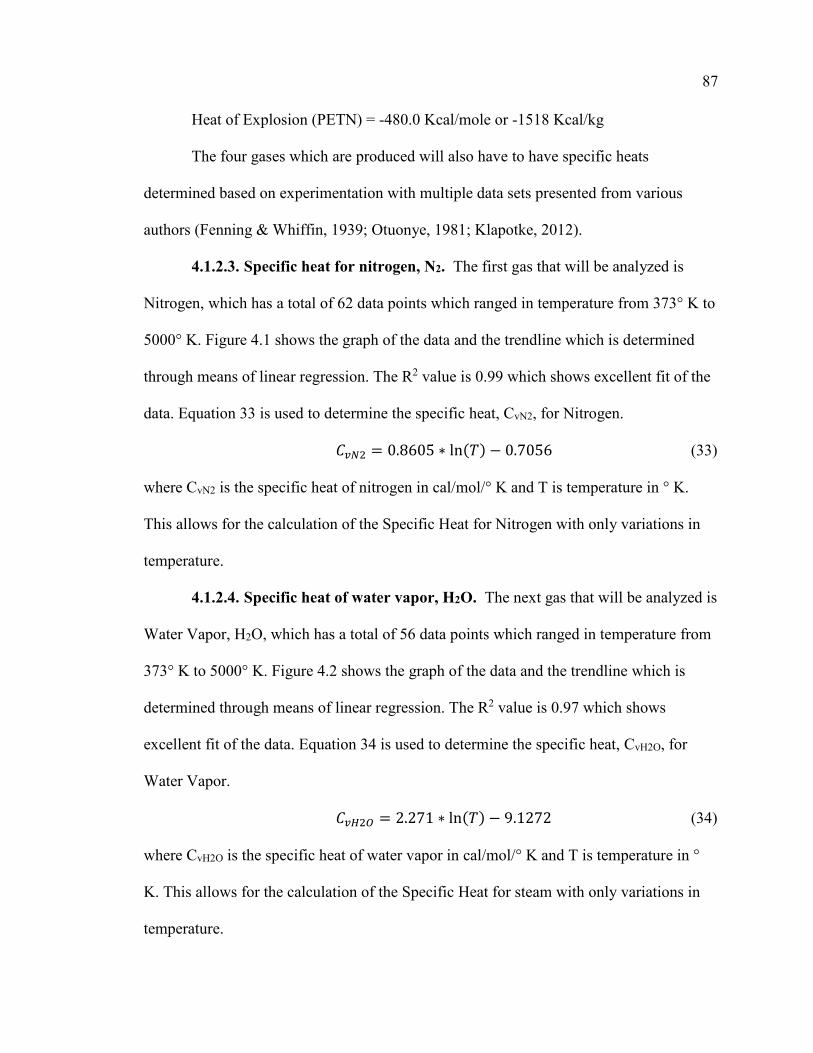
87
Heat of Explosion (PETN) = -480.0 Kcal/mole or -1518 Kcal/kg
The four gases which are produced will also have to have specific heats
determined based on experimentation with multiple data sets presented from various
authors (Fenning & Whiffin, 1939; Otuonye, 1981; Klapotke, 2012).
4.1.2.3. Specific heat for nitrogen, N2. The first gas that will be analyzed is
Nitrogen, which has a total of 62 data points which ranged in temperature from 373° K to
5000° K. Figure 4.1 shows the graph of the data and the trendline which is determined
through means of linear regression. The R2 value is 0.99 which shows excellent fit of the
data. Equation 33 is used to determine the specific heat, CvN2, for Nitrogen.
𝐶𝐶𝑣𝑣𝑁𝑁2 = 0.8605 ∗ ln(𝑇𝑇) − 0.7056 (33)
where CvN2 is the specific heat of nitrogen in cal/mol/° K and T is temperature in ° K.
This allows for the calculation of the Specific Heat for Nitrogen with only variations in
temperature.
4.1.2.4. Specific heat of water vapor, H2O. The next gas that will be analyzed is
Water Vapor, H2O, which has a total of 56 data points which ranged in temperature from
373° K to 5000° K. Figure 4.2 shows the graph of the data and the trendline which is
determined through means of linear regression. The R2 value is 0.97 which shows
excellent fit of the data. Equation 34 is used to determine the specific heat, CvH2O, for
Water Vapor.
𝐶𝐶𝑣𝑣𝐻𝐻2𝑂𝑂 = 2.271 ∗ ln(𝑇𝑇) − 9.1272 (34)
where CvH2O is the specific heat of water vapor in cal/mol/° K and T is temperature in °
K. This allows for the calculation of the Specific Heat for steam with only variations in
temperature.
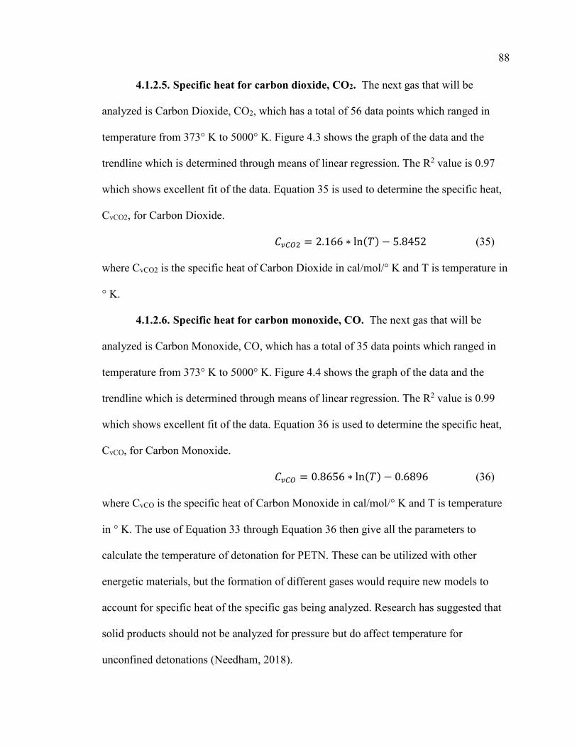
88
4.1.2.5. Specific heat for carbon dioxide, CO2. The next gas that will be
analyzed is Carbon Dioxide, CO2, which has a total of 56 data points which ranged in
temperature from 373° K to 5000° K. Figure 4.3 shows the graph of the data and the
trendline which is determined through means of linear regression. The R2 value is 0.97
which shows excellent fit of the data. Equation 35 is used to determine the specific heat,
CvCO2, for Carbon Dioxide.
𝐶𝐶𝑣𝑣𝐶𝐶𝑂𝑂2 = 2.166 ∗ ln(𝑇𝑇) − 5.8452 (35)
where CvCO2 is the specific heat of Carbon Dioxide in cal/mol/° K and T is temperature in
° K.
4.1.2.6. Specific heat for carbon monoxide, CO. The next gas that will be
analyzed is Carbon Monoxide, CO, which has a total of 35 data points which ranged in
temperature from 373° K to 5000° K. Figure 4.4 shows the graph of the data and the
trendline which is determined through means of linear regression. The R2 value is 0.99
which shows excellent fit of the data. Equation 36 is used to determine the specific heat,
CvCO, for Carbon Monoxide.
𝐶𝐶𝑣𝑣𝐶𝐶𝑂𝑂 = 0.8656 ∗ ln(𝑇𝑇) − 0.6896 (36)
where CvCO is the specific heat of Carbon Monoxide in cal/mol/° K and T is temperature
in ° K. The use of Equation 33 through Equation 36 then give all the parameters to
calculate the temperature of detonation for PETN. These can be utilized with other
energetic materials, but the formation of different gases would require new models to
account for specific heat of the specific gas being analyzed. Research has suggested that
solid products should not be analyzed for pressure but do affect temperature for
unconfined detonations (Needham, 2018).
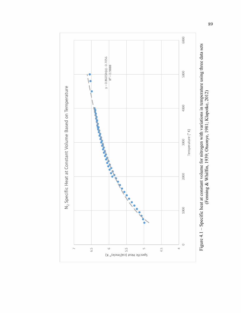
89
Figu
re 4
.1 –
Spe
cific
hea
t at c
onst
ant v
olum
e fo
r nitr
ogen
with
var
iatio
ns in
tem
pera
ture
usi
ng th
ree
data
sets
(F
enni
ng &
Whi
ffin,
193
9; O
tuon
ye, 1
981;
Kla
potk
e, 2
012)

90
Figu
re 4
.2 –
Spe
cific
hea
t at c
onst
ant v
olum
e fo
r wat
er v
apor
with
var
iatio
ns to
tem
pera
ture
usi
ng th
ree
data
sets
(F
enni
ng &
Whi
ffin,
193
9; O
tuon
ye, 1
981;
Kla
potk
e, 2
012)

91
Figu
re 4
.3 -
Spec
ific
heat
at c
onst
ant v
olum
e fo
r car
bon
diox
ide
with
var
iatio
ns to
tem
pera
ture
usi
ng th
ree
data
se
ts (F
enni
ng &
Whi
ffin,
193
9; O
tuon
ye, 1
981;
Kla
potk
e, 2
012)

92
Figu
re 4
.4 –
Spe
cific
hea
t at c
onst
ant v
olum
e fo
r car
bon
mon
oxid
e w
ith v
aria
tions
to te
mpe
ratu
re u
sing
one
dat
a se
t (K
lapo
tke,
201
2)
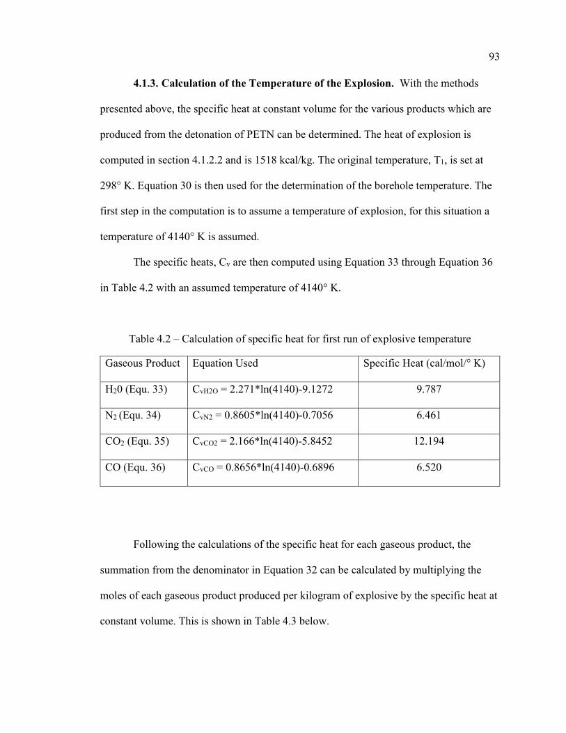
93
4.1.3. Calculation of the Temperature of the Explosion. With the methods
presented above, the specific heat at constant volume for the various products which are
produced from the detonation of PETN can be determined. The heat of explosion is
computed in section 4.1.2.2 and is 1518 kcal/kg. The original temperature, T1, is set at
298° K. Equation 30 is then used for the determination of the borehole temperature. The
first step in the computation is to assume a temperature of explosion, for this situation a
temperature of 4140° K is assumed.
The specific heats, Cv are then computed using Equation 33 through Equation 36
in Table 4.2 with an assumed temperature of 4140° K.
Table 4.2 – Calculation of specific heat for first run of explosive temperature
Gaseous Product Equation Used Specific Heat (cal/mol/° K)
H20 (Equ. 33) CvH2O = 2.271*ln(4140)-9.1272 9.787
N2 (Equ. 34) CvN2 = 0.8605*ln(4140)-0.7056 6.461
CO2 (Equ. 35) CvCO2 = 2.166*ln(4140)-5.8452 12.194
CO (Equ. 36) CvCO = 0.8656*ln(4140)-0.6896 6.520
Following the calculations of the specific heat for each gaseous product, the
summation from the denominator in Equation 32 can be calculated by multiplying the
moles of each gaseous product produced per kilogram of explosive by the specific heat at
constant volume. This is shown in Table 4.3 below.
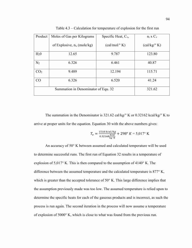
94
Table 4.3 – Calculation for temperature of explosion for the first run
Product Moles of Gas per Kilograms
of Explosive, ni, (mole/kg)
Specific Heat, Cv,
(cal/mol/° K)
ni x Cv
(cal/kg/° K)
H20 12.65 9.787 123.80
N2 6.326 6.461 40.87
CO2 9.489 12.194 115.71
CO 6.326 6.520 41.24
Summation in Denominator of Equ. 32 321.62
The summation in the Denominator is 321.62 cal/kg/° K or 0.32162 kcal/kg/° K to
arrive at proper units for the equation. Equation 30 with the above numbers gives:
𝑇𝑇𝑒𝑒 = 1518 𝑘𝑘𝑐𝑐𝑘𝑘𝑘𝑘/𝑘𝑘𝑔𝑔
0.32168 𝑘𝑘𝑐𝑐𝑎𝑎𝑘𝑘𝑘𝑘𝑔𝑔 °𝐾𝐾
+ 298° 𝐾𝐾 = 5,017° K
An accuracy of 50° K between assumed and calculated temperature will be used
to determine successful runs. The first run of Equation 32 results in a temperature of
explosion of 5,017° K. This is then compared to the assumption of 4140° K. The
difference between the assumed temperature and the calculated temperature is 877° K,
which is greater than the accepted tolerance of 50° K. This large difference implies that
the assumption previously made was too low. The assumed temperature is relied upon to
determine the specific heats for each of the gaseous products and is incorrect, as such the
process is run again. The second iteration in the process will now assume a temperature
of explosion of 5000° K, which is close to what was found from the previous run.
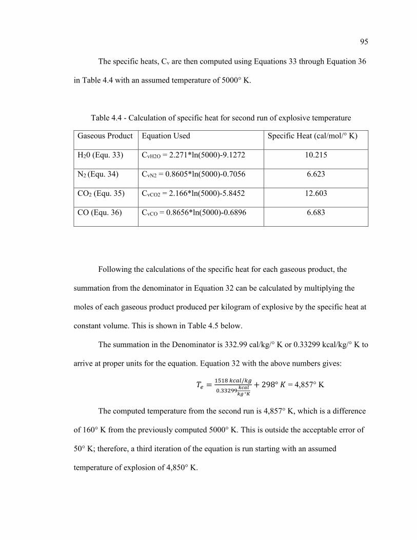
95
The specific heats, Cv are then computed using Equations 33 through Equation 36
in Table 4.4 with an assumed temperature of 5000° K.
Table 4.4 - Calculation of specific heat for second run of explosive temperature
Gaseous Product Equation Used Specific Heat (cal/mol/° K)
H20 (Equ. 33) CvH2O = 2.271*ln(5000)-9.1272 10.215
N2 (Equ. 34) CvN2 = 0.8605*ln(5000)-0.7056 6.623
CO2 (Equ. 35) CvCO2 = 2.166*ln(5000)-5.8452 12.603
CO (Equ. 36) CvCO = 0.8656*ln(5000)-0.6896 6.683
Following the calculations of the specific heat for each gaseous product, the
summation from the denominator in Equation 32 can be calculated by multiplying the
moles of each gaseous product produced per kilogram of explosive by the specific heat at
constant volume. This is shown in Table 4.5 below.
The summation in the Denominator is 332.99 cal/kg/° K or 0.33299 kcal/kg/° K to
arrive at proper units for the equation. Equation 32 with the above numbers gives:
𝑇𝑇𝑒𝑒 = 1518 𝑘𝑘𝑐𝑐𝑘𝑘𝑘𝑘/𝑘𝑘𝑔𝑔
0.33299 𝑘𝑘𝑐𝑐𝑎𝑎𝑘𝑘𝑘𝑘𝑔𝑔 °𝐾𝐾
+ 298° 𝐾𝐾 = 4,857° K
The computed temperature from the second run is 4,857° K, which is a difference
of 160° K from the previously computed 5000° K. This is outside the acceptable error of
50° K; therefore, a third iteration of the equation is run starting with an assumed
temperature of explosion of 4,850° K.

96
Table 4.5 – Calculation for temperature of explosion second run
Product Moles of Gas per Kilograms
of Explosive, ni, (mole/kg)
Specific Heat, Cv,
(cal/mol/° K)
ni x Cv
(cal/kg/° K)
H20 12.65 10.215 129.22
N2 6.326 6.623 41.90
CO2 9.489 12.603 119.59
CO 6.326 6.683 42.28
Summation in Denominator of Equ. 32 332.99
The specific heats, Cv are then computed using Equations 33 through Equations
36 in Table 4.6 with an assumed temperature of 4850° K. The calculated specific heats
show less deviation from the previous run, showing that the process is converging.
Table 4.6 - Calculation of specific heat for third run of explosive temperature
Gaseous Product Equation Used Specific Heat (cal/mol/° K)
H20 (Equ. 33) CvH2O = 2.271*ln(4850)-9.1272 10.146
N2 (Equ. 34) CvN2 = 0.8605*ln(4850)-0.7056 6.597
CO2 (Equ. 35) CvCO2 = 2.166*ln(4850)-5.8452 12.537
CO (Equ. 36) CvCO = 0.8656*ln(4850)-0.6896 6.657

97
Following the calculations of the specific heat for each gaseous product, the
summation from the denominator in Equation 32 can be calculated by multiplying the
moles of each gaseous product produced per kilogram of explosive by the specific heat at
constant volume. This is shown in Table 4.7 below.
Table 4.7 – Calculation for temperature of explosion third run
Product Moles of Gas per Kilograms
of Explosive, ni, (mole/kg)
Specific Heat, Cv,
(cal/mol/° K)
ni x Cv
(cal/kg/° K)
H20 12.65 10.146 128.35
N2 6.326 6.597 41.73
CO2 9.489 12.537 118.96
CO 6.326 6.657 42.11
Summation in Denominator of Equ. 32 331.16
The summation in the Denominator is 331.16 cal/kg/° K or 0.33116 kcal/kg/° K to
arrive at proper units for the equation. Equation 32 with the above numbers gives:
𝑇𝑇𝑒𝑒 = 1518 𝑘𝑘𝑐𝑐𝑘𝑘𝑘𝑘/𝑘𝑘𝑔𝑔
0.33116 𝑘𝑘𝑐𝑐𝑎𝑎𝑘𝑘𝑘𝑘𝑔𝑔 °𝐾𝐾
+ 298° 𝐾𝐾 = 4,882° K
The temperature of detonation after the third iteration of Equation 32 yields a
temperature of 4,882° K, which is a difference of 25° K from the second iteration
temperature of 4857° K. This is within the acceptable tolerance of 50° K. The
temperature of detonation for PETN is 4,900° K.
98
This method of determining the temperature of the explosion is a reliable method
which works for high explosives. From the author’s previous work, this system does not
seem to work as well for low explosives which deflagrate dramatically over-estimating
the results. This would then only be recommended for detonating explosives. The major
challenge with this system is the proper computation of the specific heat for all products
as information is scare for the specific heats at these temperatures.
4.2. DETONATION PRESSURE MODEL
The detonation pressure model will utilize a base equation of state from previous
research to determine the borehole pressure for variations in explosives.
4.2.1. Validation of Equations of State from Experimental Data. The
development of the temperature of the explosion gives the ability to analyze the
previously presented Equations of State (EOS) for the determination of the explosive
pressures when the gas is in the same volume as the original explosive. These are
presented below to facilitate easy referencing as Equations 37 through Equations 43. The
BWS Equation of State is:
𝑃𝑃𝑒𝑒 = 𝜌𝜌𝜌𝜌𝜌𝜌𝑇𝑇𝑒𝑒�1 + 𝑥𝑥𝑒𝑒𝛽𝛽𝛽𝛽� (37)
𝑥𝑥 = 𝜌𝜌𝜌𝜌(𝑇𝑇𝑒𝑒 + 𝜃𝜃)−𝛼𝛼 (38)
where Pe is the explosive gas pressure atmospheres, ρ is the density of the explosive, n is
the moles of gas, R is the gas constant, Te is the temperature of detonation in degrees
Kelvin, x is a constant based on a function of the temperature of detonation, and β, k, θ,
and α are all experimentally determined constants. It has been suggested that acceptable
values for these constants are k = 1; θ = 0; α = 0.25; and β = 0.3.
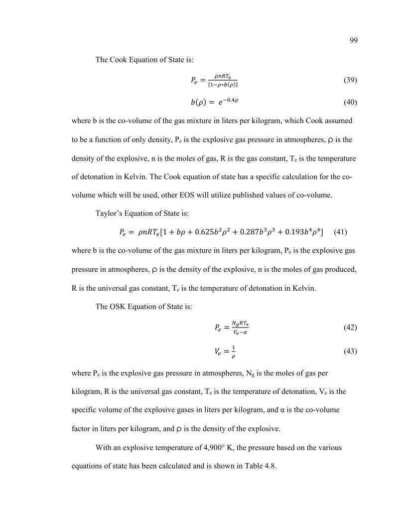
99
The Cook Equation of State is:
𝑃𝑃𝑒𝑒 = 𝜌𝜌𝜌𝜌𝜌𝜌𝑇𝑇𝑒𝑒[1−𝜌𝜌∗𝑏𝑏(𝜌𝜌)] (39)
𝑏𝑏(𝜌𝜌) = 𝑒𝑒−0.4𝜌𝜌 (40)
where b is the co-volume of the gas mixture in liters per kilogram, which Cook assumed
to be a function of only density, Pe is the explosive gas pressure in atmospheres, ρ is the
density of the explosive, n is the moles of gas, R is the gas constant, Te is the temperature
of detonation in Kelvin. The Cook equation of state has a specific calculation for the co-
volume which will be used, other EOS will utilize published values of co-volume.
Taylor’s Equation of State is:
𝑃𝑃𝑒𝑒 = 𝜌𝜌𝜌𝜌𝜌𝜌𝑇𝑇𝑒𝑒[1 + 𝑏𝑏𝜌𝜌 + 0.625𝑏𝑏2𝜌𝜌2 + 0.287𝑏𝑏3𝜌𝜌3 + 0.193𝑏𝑏4𝜌𝜌4] (41)
where b is the co-volume of the gas mixture in liters per kilogram, Pe is the explosive gas
pressure in atmospheres, ρ is the density of the explosive, n is the moles of gas produced,
R is the universal gas constant, Te is the temperature of detonation in Kelvin.
The OSK Equation of State is:
𝑃𝑃𝑒𝑒 = 𝑁𝑁𝑔𝑔𝜌𝜌𝑇𝑇𝑒𝑒𝑉𝑉𝑒𝑒−𝛼𝛼
(42)
𝑉𝑉𝑒𝑒 = 1𝜌𝜌 (43)
where Pe is the explosive gas pressure in atmospheres, Ng is the moles of gas per
kilogram, R is the universal gas constant, Te is the temperature of detonation, Ve is the
specific volume of the explosive gases in liters per kilogram, and α is the co-volume
factor in liters per kilogram, and ρ is the density of the explosive.
With an explosive temperature of 4,900° K, the pressure based on the various
equations of state has been calculated and is shown in Table 4.8.
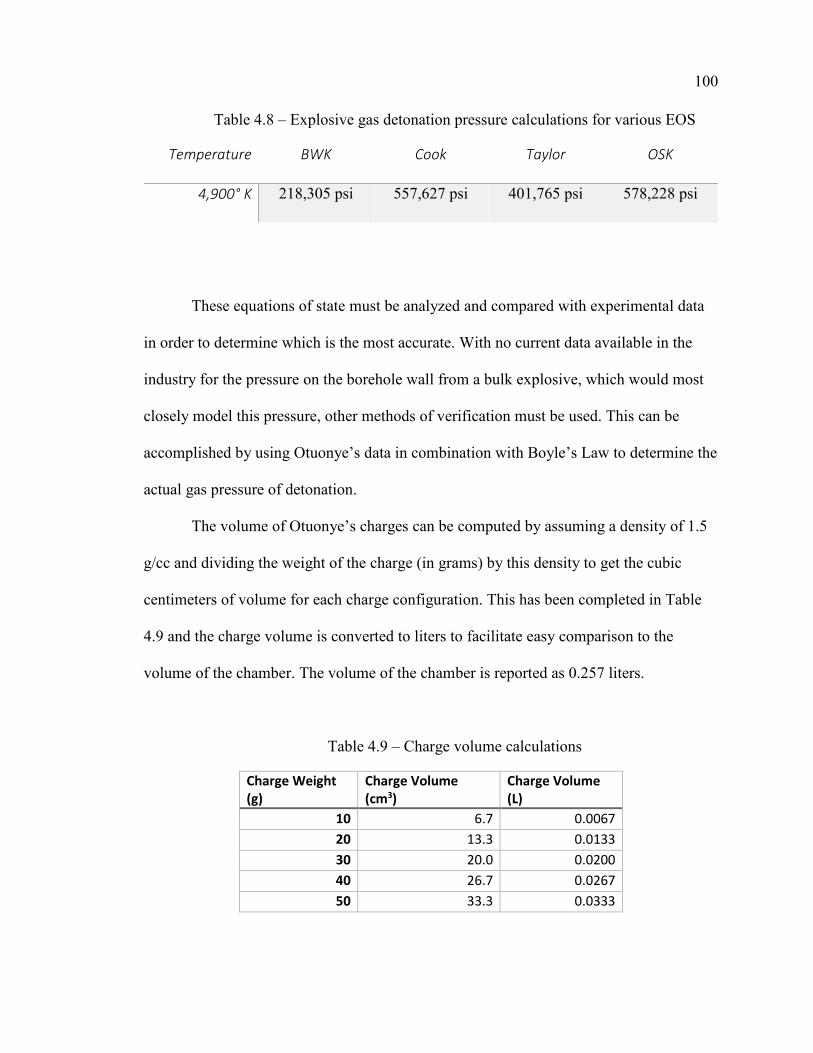
100
Table 4.8 – Explosive gas detonation pressure calculations for various EOS
Temperature BWK Cook Taylor OSK
4,900° K 218,305 psi 557,627 psi 401,765 psi 578,228 psi
These equations of state must be analyzed and compared with experimental data
in order to determine which is the most accurate. With no current data available in the
industry for the pressure on the borehole wall from a bulk explosive, which would most
closely model this pressure, other methods of verification must be used. This can be
accomplished by using Otuonye’s data in combination with Boyle’s Law to determine the
actual gas pressure of detonation.
The volume of Otuonye’s charges can be computed by assuming a density of 1.5
g/cc and dividing the weight of the charge (in grams) by this density to get the cubic
centimeters of volume for each charge configuration. This has been completed in Table
4.9 and the charge volume is converted to liters to facilitate easy comparison to the
volume of the chamber. The volume of the chamber is reported as 0.257 liters.
Table 4.9 – Charge volume calculations
Charge Weight (g)
Charge Volume (cm3)
Charge Volume (L)
10 6.7 0.0067 20 13.3 0.0133 30 20.0 0.0200 40 26.7 0.0267 50 33.3 0.0333
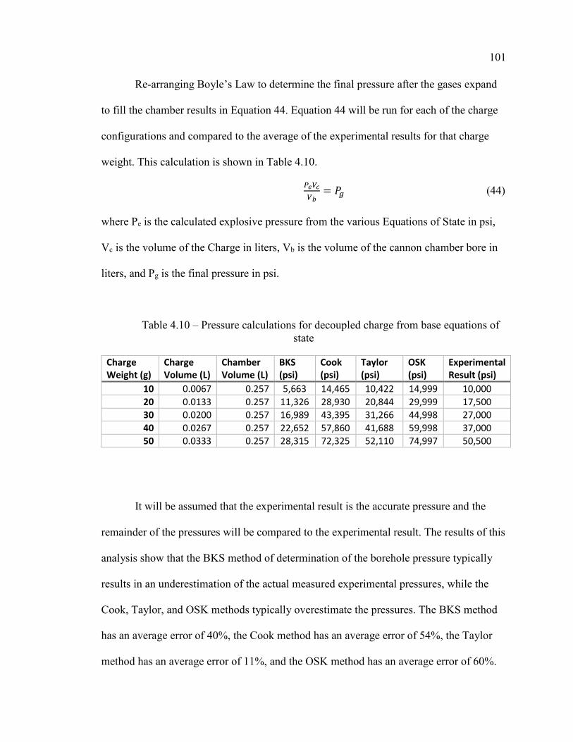
101
Re-arranging Boyle’s Law to determine the final pressure after the gases expand
to fill the chamber results in Equation 44. Equation 44 will be run for each of the charge
configurations and compared to the average of the experimental results for that charge
weight. This calculation is shown in Table 4.10.
𝑃𝑃𝑒𝑒𝑉𝑉𝑐𝑐𝑉𝑉𝑏𝑏
= 𝑃𝑃𝑔𝑔 (44)
where Pe is the calculated explosive pressure from the various Equations of State in psi,
Vc is the volume of the Charge in liters, Vb is the volume of the cannon chamber bore in
liters, and Pg is the final pressure in psi.
Table 4.10 – Pressure calculations for decoupled charge from base equations of state
Charge Weight (g)
Charge Volume (L)
Chamber Volume (L)
BKS (psi)
Cook (psi)
Taylor (psi)
OSK (psi)
Experimental Result (psi)
10 0.0067 0.257 5,663 14,465 10,422 14,999 10,000 20 0.0133 0.257 11,326 28,930 20,844 29,999 17,500 30 0.0200 0.257 16,989 43,395 31,266 44,998 27,000 40 0.0267 0.257 22,652 57,860 41,688 59,998 37,000 50 0.0333 0.257 28,315 72,325 52,110 74,997 50,500
It will be assumed that the experimental result is the accurate pressure and the
remainder of the pressures will be compared to the experimental result. The results of this
analysis show that the BKS method of determination of the borehole pressure typically
results in an underestimation of the actual measured experimental pressures, while the
Cook, Taylor, and OSK methods typically overestimate the pressures. The BKS method
has an average error of 40%, the Cook method has an average error of 54%, the Taylor
method has an average error of 11%, and the OSK method has an average error of 60%.
102
The Taylor Equation of State will then be considered the most accurate of the four
methods and will be used in further analysis.
As this analysis is completed, it is important to note that one of the reasons that
other methods of pressure determination significantly overestimate the pressure is
because this analysis has not taken the compressibility of the gases into account. As the
decoupling ratio decreases, the gases are compressed to a larger degree which leads to an
increase in pressure. This can be ignored for further analysis from the detonation pressure
if the decoupling ratio remains large (which is defined as a decoupling ratio greater than
three) but allows for determination of the borehole pressure from any explosive. The
compressibility will dramatically increase pressure at small decoupling ratios.
4.2.2. Development of Detonation Pressure Model from Taylor EOS. In order
to develop a model from the Taylor Equation of State for a charge of any explosive type
which has large decoupling, the blasting process is extremely rapid and is assumed to be
adiabatic. This results in no heat transfer of the explosive gases to the rock mass.
Furthermore, due to the rapid expansion of gases and the stagnation temperature of gas
collision on the borehole wall, it is assumed that the process is isothermal (Otuonye,
Skidmore, & Konya, 1983) resulting in minimal change to the gas temperature.
The assumption that the process is isothermal does not represent actual field
conditions but is a simplified modelling approach which presents minimal errors in the
total magnitude of calculations. The temperature losses associated in the gas are minimal
from the detonation, through expansion, to arrival of the maximum borehole pressure.
This is due to the cooling effect of the gas during expansion being offset by the increase
in the gas temperature from the stagnation of the gases at the borehole wall, which would

103
be assumed to be completed as the maximum pressure is reached. Following the
maximum pressure, the process can not be treated as isothermal.
Furthermore, modelling of the process as an isothermal reaction for decoupled
charges has shown a good fit to experimental data (Otuonye, Skidmore, & Konya, 1983).
The theoretical treatment of this can also be completed using the mechanism of
rarefaction gases cooling in a vacuum (Molmud, 1960). Under this modelling the rate of
cooling would result in a change of temperature of approximately 100° K to 150° K,
which is approximately 3% of the detonation temperature. The completion of a sensitivity
analysis shows that a loss of temperature minimally effects the borehole pressure. For
example, a loss of 100° K would result in a 2% change in the borehole pressure. Due to
the minimal changes in temperature from a theoretical perspective, the accurate
modelling of field data based on isothermal assumptions, and the minimal sensitivity of
the changes in temperature to the pressure, the process will be modeled as an isothermal
process. A full justification of the isothermal assumption can be found in appendix three.
Boyle’s law can then be applied which relates initial pressure and volume to the
final pressure and volume. Equation 45 is Boyle’s Law (Equation 26) which has been
modified to isolate the final pressure, or the borehole pressure, and had blasting specific
terms substituted.
𝑃𝑃𝑔𝑔 = 𝑃𝑃𝑇𝑇𝑉𝑉𝑒𝑒𝑉𝑉𝑏𝑏
(45)
where Pg is the borehole gas pressure in psi, PT is the explosive pressure from Taylors
Equation (Equation 41) in psi, Ve is the volume of the explosive charge in liters, and Vb is
the volume of the borehole in liters.

104
The volume of the borehole can be modeled as the volume of a cylinder.
Modifications to this equation to include blasting specific terms and facilitate common
field units have been completed and are present in Equation 46.
𝑉𝑉𝑏𝑏 = 0.156𝑑𝑑ℎ2𝑃𝑃𝐶𝐶 (46)
where Vb is the volume of the borehole in liters, dh is the diameter of the borehole in
inches, and PC is the length of the powder column in feet.
The volume of the explosive can be calculated based on the total weight of the
explosive in grams divided by the density in grams per cubic centimeter of the explosive.
The weight of the explosive is equivalent to the explosive load in grams per meter of
boreholes multiplied by the powder column.
This gives the volume of the explosive in the form of Equation 47.
𝑉𝑉𝑒𝑒 = 𝐸𝐸𝐸𝐸∗𝑃𝑃𝐶𝐶𝜌𝜌
(47)
where the Ve is the volume of the explosive is in cubic centimeters, EL is the explosive
load in grams per meter, PC is the length of the powder column in meters, and ρ is the
density of the explosive in grams per cubic centimeter.
Equation 46 can then be converted to typical field blasting units in the imperial
system to facilitate ease of use. The conversion of Equation 47 leads to Equation 48.
𝑉𝑉𝑒𝑒 = 0.454∗𝐸𝐸𝐸𝐸∗𝑃𝑃𝐶𝐶𝜌𝜌
(48)
where Ve is the volume of the explosive in liters, EL is the explosive load in pounds per
foot, PC is the powder column length in feet, and ρ is the density of the explosive in
grams per cubic centimeter. The density in Equation 47 is technically written in metric
units and in imperial units would be termed the specific gravity of the explosive;
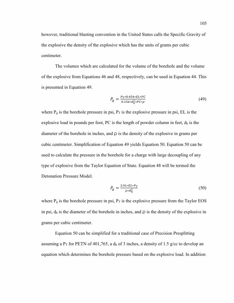
105
however, traditional blasting convention in the United States calls the Specific Gravity of
the explosive the density of the explosive which has the units of grams per cubic
centimeter.
The volumes which are calculated for the volume of the borehole and the volume
of the explosive from Equations 46 and 48, respectively, can be used in Equation 44. This
is presented in Equation 49.
𝑃𝑃𝑔𝑔 = 𝑃𝑃𝑇𝑇∗0.454∗𝐸𝐸𝐸𝐸∗𝑃𝑃𝐶𝐶0.156∗𝑑𝑑ℎ
2∗𝑃𝑃𝐶𝐶∗𝜌𝜌 (49)
where Pg is the borehole pressure in psi, PT is the explosive pressure in psi, EL is the
explosive load in pounds per foot, PC is the length of powder column in feet, dh is the
diameter of the borehole in inches, and ρ is the density of the explosive in grams per
cubic centimeter. Simplification of Equation 49 yields Equation 50. Equation 50 can be
used to calculate the pressure in the borehole for a charge with large decoupling of any
type of explosive from the Taylor Equation of State. Equation 48 will be termed the
Detonation Pressure Model.
𝑃𝑃𝑔𝑔 = 2.91∗𝐸𝐸𝐸𝐸∗𝑃𝑃𝑇𝑇𝜌𝜌∗𝑑𝑑ℎ
2 (50)
where Pg is the borehole pressure in psi, PT is the explosive pressure from the Taylor EOS
in psi, dh is the diameter of the borehole in inches, and ρ is the density of the explosive in
grams per cubic centimeter.
Equation 50 can be simplified for a traditional case of Precision Presplitting
assuming a PT for PETN of 401,765, a dh of 3 inches, a density of 1.5 g/cc to develop an
equation which determines the borehole pressure based on the explosive load. In addition
106
to this, the equation can be modified to facilitate the use of the explosive load in grains
per foot. This is presented in Equation 51.
𝑃𝑃𝑔𝑔 = 12.32 ∗ 𝐸𝐸𝐸𝐸 (51)
where Pg is the borehole pressure in psi and EL is the explosive load in grains per foot.
Equation 50 can be compared to the actual measured borehole pressures by
Otuonye. This shows an average error of 13.1% with some outliers over 25%. The
empirically derived equation presented in Equation 30 can also be compared with
Equation 50 and the measured values of the borehole pressure. A graph of this is shown
in Figure 4.5. This shows that Equation 50 predicts slightly higher values for borehole
pressure than Equation 30. Equation 50 falls slightly higher than the data set, which is
due to the fact that Taylor’s Equation of State introduces additional inaccuracies.
Equation 50, the simplified Precision Presplitting pressure equation based on the
Taylor Equation of State, can also be compared to Equation 31, the simplified Precision
Presplitting pressure equation based on empirical analysis. Figure 4.6 shows this
comparison and Equation 51 typically predicts higher pressure values than Equation 31.
The major benefit of Equation 50 is in its ability to predict the borehole pressure
for any type of explosive which has a decoupling ratio greater than three. For the case of
Precision Presplitting, it seems a more accurate estimation may be made through the use
of Equation 30 and 31.
4.3. DEVELOPMENT OF THERMODYNAMIC MODEL
The previously developed models in this dissertation can be used for situations
where the decoupling ratio is above three for various types of explosives. As the
107
decoupling ratio is reduced under three, the pressure in the borehole rapidly increases.
This can be modelled by using Equation 50 and observing the effects of a decreasing
borehole diameter while keeping the explosive load constant. This effectively represents
a decreasing decoupling ratio and is shown in Figure 4.7.
Figure 4.7 shows that once a decoupling ratio is less than three, the borehole
pressure will rise dramatically while the pressure has a lesser reaction to changes in
decoupling ratio over three. The changes in pressure, at steady temperature, also cause
changes to the compressibility of the gas mixture. For example, at larger decoupling
ratios the compressibility may change by 2% for a 1.0 decrease in the decoupling ratio.
However, for an equivalent 1.0 decrease in the decoupling ratio at small values, the
compressibility may change by 20%. In the previous methods of pressure determination,
the compressibility of the gas mixture has been ignored, as it has minimal effects when
the decoupling ratio is large and significantly increases the complexity of calculations.
However, in order to develop a model which can be used for any decoupling ratio, the
compressibility should be considered.
The compressibility of a gas will be denoted as Z and can be found from
published compressibility curves for various reduced pressures and reduced temperatures
(Wark, 1988).
The Ideal Gas Law is a method of calculating the pressure of a system based on
the moles of gas produced, temperature, and volume of the container. This is a commonly
accepted method to calculate the pressure of a system; however, it cannot be applied
when the pressure and temperature are extreme because it does not consider the gas
108
compressibility. Therefore, thermodynamics has presented a simple modification to the
Ideal Gas Law which incorporates compressibility and is shown in Equation 52.
𝑃𝑃𝑉𝑉 = 𝑍𝑍𝜌𝜌𝜌𝜌𝑇𝑇 (52)
where P is the pressure in atmospheres, V is volume in liters, n is the moles of gas, T is
temperature in Kelvin, R is the universal gas constant in liters-atm per mole degree
Kelvin (this is a constant of 0.08206), and Z is the compressibility, which is unitless. The
units presented here are different than in previous sections in order to properly scale with
the compressibility.
The compression of a gas increases the pressure very rapidly as the packing
density is significantly increased and other forces begin to take effect. This results in a
high-density gas with large pressures, which is an uncommon occurrence and is rarely
treated in explosive engineering.
In order to determine the compressibility at the set temperature and pressure, the
temperature and pressure must be corrected to a reduced temperature and reduced
pressure. The reduced pressure can be calculated with Equation 53.
𝑃𝑃𝑟𝑟 = 𝑃𝑃𝑔𝑔𝑃𝑃𝑐𝑐
(53)
where Pr is the reduced pressure in psi, Pg is the borehole pressure in psi, and Pc is the
Pressure Compressibility Constant, which is different for each individual gas. The
reduced pressure of the total gas mixture can be found from Equation 54.
𝑃𝑃𝑟𝑟𝑟𝑟𝑟𝑟𝑟𝑟 = ∑𝜌𝜌𝑖𝑖𝑃𝑃𝑟𝑟𝑖𝑖 (54)
where PrMIX is the Reduced Pressure of the gas mixture, ni is the moles fraction of gas per
gram of explosive for an individual gas, and Pri is the reduced pressure for an individual
gas.
109
The reduced temperature of the mixture can be found using Equation 55.
𝑇𝑇𝑟𝑟 = 𝑇𝑇𝑒𝑒𝑇𝑇𝑐𝑐
(55)
where Tr is the reduced temperature in °K, Te is the detonation temperature in °K, and Tc
is the gas specific reduced temperature for each individual gas. The reduced temperature
of the total gas mixture can be found from Equation 56.
𝑇𝑇𝑟𝑟𝑟𝑟𝑟𝑟𝑟𝑟 = ∑𝜌𝜌𝑖𝑖𝑇𝑇𝑟𝑟𝑖𝑖 (56)
where TrMIX is the reduced temperature of the gas mixture, ni is the moles fraction of each
individual gas produced per gram of explosive, and Tri is the reduced temperature for
each individual gas.
The combination of the reduced temperature of the mixtures and the reduced
pressure of the mixture is then used to determine the compressibility.
The pressure in the borehole can then be found from application of Equation 52.
Equation 57 is the simplified form of Equation 52 to facilitate easier calculation of the
borehole pressure. Equation 57 is termed the Thermodynamic Model.
𝑃𝑃𝑔𝑔 = 14.7∗𝑍𝑍𝑐𝑐∗𝜌𝜌𝑔𝑔∗𝜌𝜌∗𝑇𝑇𝑒𝑒𝑉𝑉𝑏𝑏
(57)
where Pg is the borehole pressure in psi, Zc is the compressibility of the gas mixture, ng is
moles of gas produced in moles, R is the universal gas constant which is taken as 0.08206
liters-atm per mole degree Kelvin, Te is the detonation temperature in Kelvin, and Vb is
the volume of the borehole in liters. The moles of gas produced can be calculated using
Equation 58.
𝜌𝜌𝑔𝑔 = 454 ∗ 𝑤𝑤𝑒𝑒 ∗ 𝜌𝜌𝑟𝑟𝑟𝑟𝑟𝑟 (58)

110
where ng is the total moles of gas produced in moles, we is the weight of the explosive in
pounds, and nMIX is the moles of gas produced per gram of explosive.
The substitution of Equation 45 for the borehole volume and Equation 58 for the
moles of gas into Equation 57 yields Equation 59.
𝑃𝑃𝑔𝑔 = 3510∗𝑍𝑍𝑐𝑐∗𝑤𝑤𝑒𝑒𝜌𝜌𝑀𝑀𝑀𝑀𝑀𝑀∗𝑇𝑇𝑒𝑒𝑑𝑑ℎ2∗𝑃𝑃𝐶𝐶
(59)
where Pg is the borehole pressure in psi, Zc is the compressibility of the gas mixture, we is
the weight of the explosive in pounds, and nMIX is the moles of gas produced per gram of
explosive, Te is the detonation temperature in Kelvin, dh is the borehole diameter in
inches, and PC is the powder column in feet.
The explosive load can be written in terms of Equation 60
𝐸𝐸𝐸𝐸 = 𝑤𝑤𝑒𝑒𝑃𝑃𝐶𝐶
(60)
where EL is the explosive load in pounds per foot, we is the weight of the explosive in
pounds, and PC is the length of powder column in feet.
Equation 60 can then be substituted into Equation 59, producing Equation 61
giving an equation for the borehole pressure based on the explosive load used in the
borehole.
𝑃𝑃𝑔𝑔 = 3510∗𝑇𝑇𝑒𝑒∗𝜌𝜌𝑀𝑀𝑀𝑀𝑀𝑀∗𝐸𝐸𝐸𝐸𝑑𝑑ℎ2 ∗ 𝑍𝑍𝑐𝑐 (61)
where Pg is the borehole pressure in psi, Zc is the compressibility of the gas mixture, Te is
the detonation temperature in Kelvin, nMIX is the moles of gas produced per gram of
explosive, EL is the explosive load in pounds per foot, and dh is the borehole diameter in
inches.
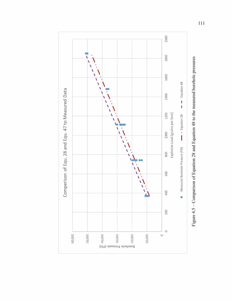
111
Figu
re 4
.5 –
Com
paris
on o
f Equ
atio
n 28
and
Equ
atio
n 48
to th
e m
easu
red
bore
hole
pre
ssur
es
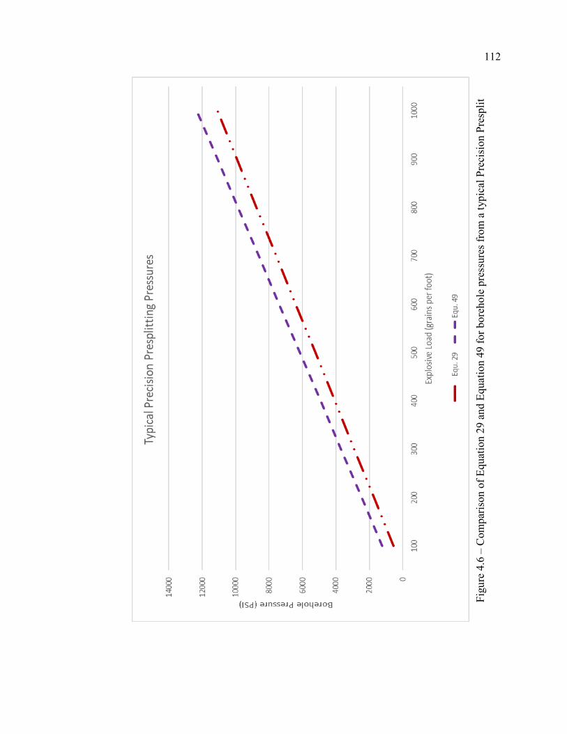
112
Figu
re 4
.6 –
Com
paris
on o
f Equ
atio
n 29
and
Equ
atio
n 49
for b
oreh
ole
pres
sure
s fro
m a
typi
cal P
reci
sion
Pre
split
b
d
li
d

113
Figu
re 4
.7 –
The
bas
ic e
ffec
ts o
f dec
oupl
ing
ratio
on
the
bore
hole
pre
ssur
e
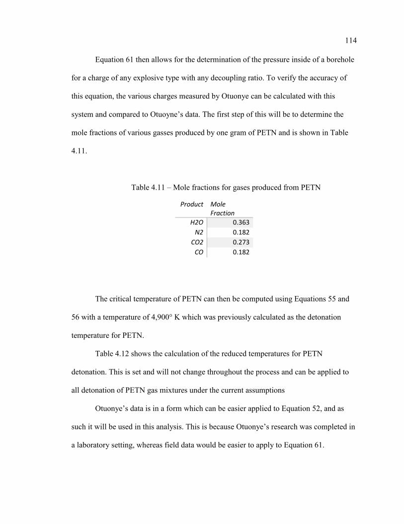
114
Equation 61 then allows for the determination of the pressure inside of a borehole
for a charge of any explosive type with any decoupling ratio. To verify the accuracy of
this equation, the various charges measured by Otuonye can be calculated with this
system and compared to Otuoyne’s data. The first step of this will be to determine the
mole fractions of various gasses produced by one gram of PETN and is shown in Table
4.11.
Table 4.11 – Mole fractions for gases produced from PETN
Product Mole Fraction
H2O 0.363 N2 0.182
CO2 0.273 CO 0.182
The critical temperature of PETN can then be computed using Equations 55 and
56 with a temperature of 4,900° K which was previously calculated as the detonation
temperature for PETN.
Table 4.12 shows the calculation of the reduced temperatures for PETN
detonation. This is set and will not change throughout the process and can be applied to
all detonation of PETN gas mixtures under the current assumptions
Otuonye’s data is in a form which can be easier applied to Equation 52, and as
such it will be used in this analysis. This is because Otuonye’s research was completed in
a laboratory setting, whereas field data would be easier to apply to Equation 61.
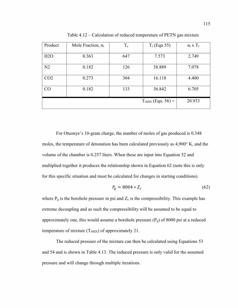
115
Table 4.12 – Calculation of reduced temperature of PETN gas mixture
Product Mole Fraction, ni Tc Tr (Equ 55) ni x Tr
H2O 0.363 647 7.573 2.749
N2 0.182 126 38.889 7.078
CO2 0.273 304 16.118 4.400
CO 0.182 133 36.842 6.705
TrMIX (Equ. 56) = 20.933
For Otuonye’s 10-gram charge, the number of moles of gas produced is 0.348
moles, the temperature of detonation has been calculated previously as 4,900° K, and the
volume of the chamber is 0.257 liters. When these are input into Equation 52 and
multiplied together it produces the relationship shown in Equation 62 (note this is only
for this specific situation and must be calculated for changes in starting conditions).
𝑃𝑃𝑔𝑔 = 8004 ∗ 𝑍𝑍𝑐𝑐 (62)
where Pg is the borehole pressure in psi and Zc is the compressibility. This example has
extreme decoupling and as such the compressibility will be assumed to be equal to
approximately one, this would assume a borehole pressure (Pg) of 8000 psi at a reduced
temperature of mixture (TrMIX) of approximately 21.
The reduced pressure of the mixture can then be calculated using Equations 53
and 54 and is shown in Table 4.13. The reduced pressure is only valid for the assumed
pressure and will change through multiple iterations.
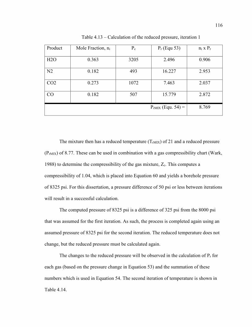
116
Table 4.13 – Calculation of the reduced pressure, iteration 1
Product Mole Fraction, ni Pc Pr (Equ 53) ni x Pr
H2O 0.363 3205 2.496 0.906
N2 0.182 493 16.227 2.953
CO2 0.273 1072 7.463 2.037
CO 0.182 507 15.779 2.872
PrMIX (Equ. 54) = 8.769
The mixture then has a reduced temperature (TrMIX) of 21 and a reduced pressure
(PrMIX) of 8.77. These can be used in combination with a gas compressibility chart (Wark,
1988) to determine the compressibility of the gas mixture, Zc. This computes a
compressibility of 1.04, which is placed into Equation 60 and yields a borehole pressure
of 8325 psi. For this dissertation, a pressure difference of 50 psi or less between iterations
will result in a successful calculation.
The computed pressure of 8325 psi is a difference of 325 psi from the 8000 psi
that was assumed for the first iteration. As such, the process is completed again using an
assumed pressure of 8325 psi for the second iteration. The reduced temperature does not
change, but the reduced pressure must be calculated again.
The changes to the reduced pressure will be observed in the calculation of Pr for
each gas (based on the pressure change in Equation 53) and the summation of these
numbers which is used in Equation 54. The second iteration of temperature is shown in
Table 4.14.

117
Table 4.14 – Calculation of reduced pressure, iteration 2
Product Mole Fraction, ni Pc Pr (Equ 53) ni x Pr
H2O 0.363 3205 2.598 0.943
N2 0.182 493 16.886 3.073
CO2 0.273 1072 7.766 2.120
CO 0.182 507 16.420 2.988
PrMIX (Equ. 54) = 9.125
The mixture then has a reduced temperature (TrMIX) of 21 and a reduced pressure
(PrMIX) of 9.125 which yields a compressibility of 1.05.
A compressibility of 1.05 in Equation 62 yields a pressure of 8400 psi. A
calculated pressure of 8400 psi from iteration two is a 75 psi difference from the assumed
pressure of 8325 psi.
For the purposes of this dissertation, a pressure difference of 50 psi of less
between iterations will results in a successful calculation. As such a third iteration of the
process is completed using an assumed pressure of 8400 psi.
The reduced pressure will be calculated again for the updated pressure
assumption. The results of the reduced pressure calculation are shown in Table 4.15. The
mixture then has a reduced temperature (TrMIX) of 21 and a reduced pressure (PrMIX) of
9.125 which yields a compressibility of 1.05. A compressibility of 1.05 in Equation 62
yields a pressure of 8400 psi which is equal to the starting assumed value. As such, the
process is completed, and the borehole pressure is calculated to be 8,400 psi.
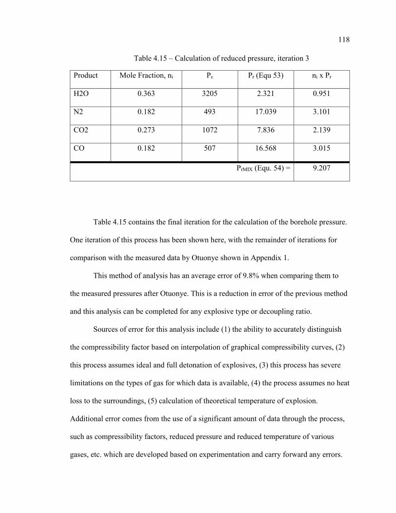
118
Table 4.15 – Calculation of reduced pressure, iteration 3
Product Mole Fraction, ni Pc Pr (Equ 53) ni x Pr
H2O 0.363 3205 2.321 0.951
N2 0.182 493 17.039 3.101
CO2 0.273 1072 7.836 2.139
CO 0.182 507 16.568 3.015
PrMIX (Equ. 54) = 9.207
Table 4.15 contains the final iteration for the calculation of the borehole pressure.
One iteration of this process has been shown here, with the remainder of iterations for
comparison with the measured data by Otuonye shown in Appendix 1.
This method of analysis has an average error of 9.8% when comparing them to
the measured pressures after Otuonye. This is a reduction in error of the previous method
and this analysis can be completed for any explosive type or decoupling ratio.
Sources of error for this analysis include (1) the ability to accurately distinguish
the compressibility factor based on interpolation of graphical compressibility curves, (2)
this process assumes ideal and full detonation of explosives, (3) this process has severe
limitations on the types of gas for which data is available, (4) the process assumes no heat
loss to the surroundings, (5) calculation of theoretical temperature of explosion.
Additional error comes from the use of a significant amount of data through the process,
such as compressibility factors, reduced pressure and reduced temperature of various
gases, etc. which are developed based on experimentation and carry forward any errors.

119
While this method has appreciable sources of error, Figure 4.8 better illustrates
that the model falls at approximate average values of the measured pressures found by
Otuonye. This indicates that while some error is found in the model to actual field
conditions, this model is excellent at predicting a typical borehole pressure for that charge
type.
In order to simplify this method of calculation, a general formula is developed
which applies to the traditional case of Precision Presplitting. Equation 58 can be
simplified for the case of blasting with PETN explosives by substituting in the detonation
temperature of 4,900° K and the moles of gas per gram of explosive produced as 0.0348.
This results in Equation 63 for determination of the borehole pressure from a PETN
based explosive.
𝑃𝑃𝑔𝑔 = 85.5∗𝑍𝑍𝑐𝑐∗𝐸𝐸𝐸𝐸𝑑𝑑ℎ2 (63)
where Pg is the borehole pressure in psi, Zc is the compressibility factor, EL is the
explosive load in grains per foot, and dh is the borehole diameter in inches.
The application of Equation 63 at the typical Precision Presplit design of a 3”
diameter borehole can be modelled to determine the relationship between the
compressibility and the explosive load of the charge. This has been completed in Figure
4.9 which shows that the compressibility varies linearly with the explosive load for
Precision Presplitting and has an excellent coefficient of correlation with an R2 factor of
0.98 and results in the development of Equation 64.
𝑍𝑍𝑐𝑐 = 0.00008 ∗ 𝐸𝐸𝐸𝐸 + 1.0 (64)
where Zc is the compressibility and EL is the explosive load in grains per foot.

120
Equation 64 can be substituted into Equation 61 and the borehole diameter can be
set at three inches to simplify an equation to determine the borehole pressure based on the
explosive load. This results in a simplified thermodynamic model for a typical Precision
Presplit which is shown in Equation 65.
𝑃𝑃𝑔𝑔 = 0.00076 ∗ 𝐸𝐸𝐸𝐸2 + 9.5𝐸𝐸𝐸𝐸 (65)
where Pg is the borehole pressure in psi and EL is the explosive load in grains per foot.
The Detonation Pressure Model is a theoretical model which can compute the
borehole pressure based on variations in the explosive, which is one of the limitations of
the Empirical Model. The Detonation Pressure model can only be used for large
decoupling ratios, a decoupling ratio greater than three, as it does not take compressibility
into account. The Detonation Pressure Model is more complex than the Empirical Model
but is a straightforward calculation when assuming an appropriate co-volume factor.
The Thermodynamic Model is a complex model which revolves around numerous
iterations and requires more complex information for various gases than the Detonation
Pressure Model. The Thermodynamic Model can be used for variations in explosive type
and decoupling ratio.
This gives the Thermodynamic Model the most flexibility of all the borehole
pressure models presented. The flexibility of the model to apply for all field blasting
situations is the most important consideration for the development of a general method of
pressure predictions. This gives it the ability to be applied to all field loading situations
for presplitting and over forms of blasting. The next important parameter is to determine
how these models function with valid data and in comparison.
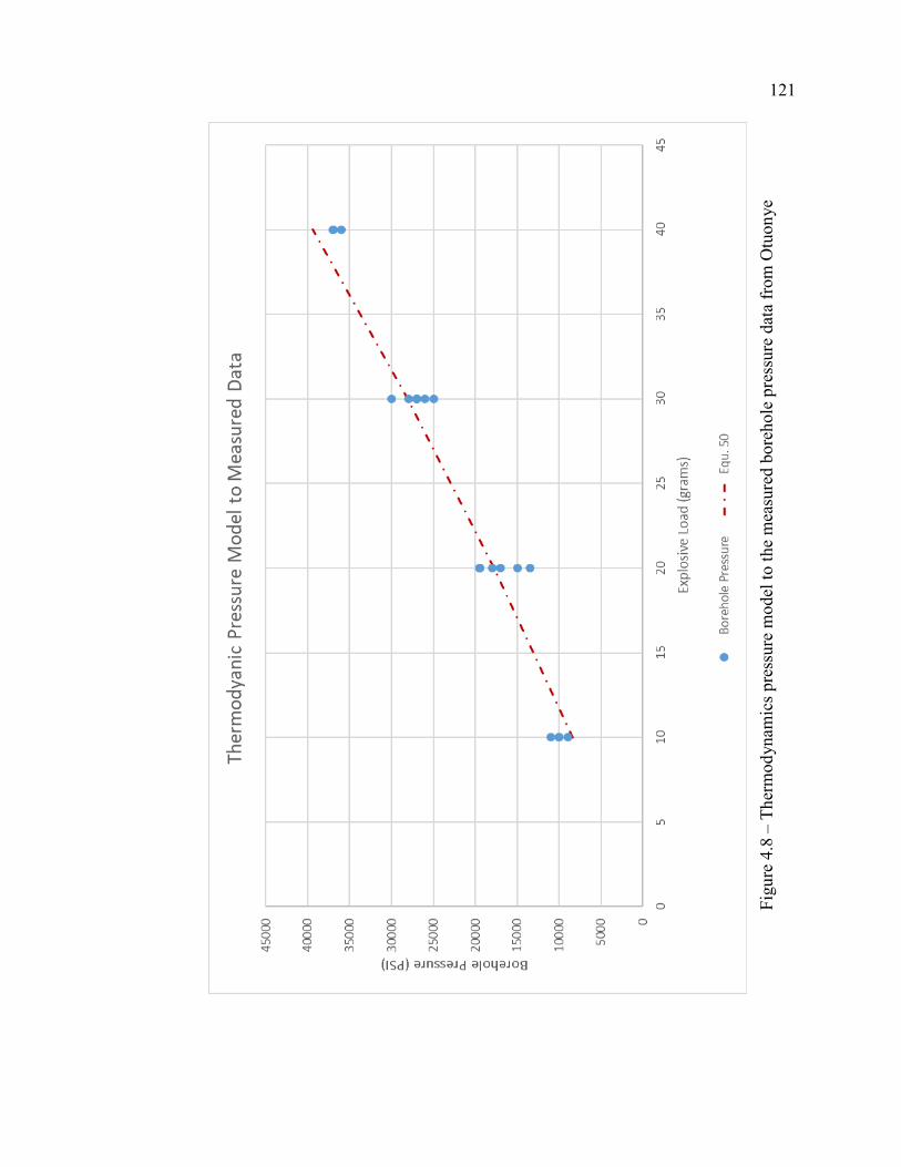
121
Figu
re 4
.8 –
The
rmod
ynam
ics p
ress
ure
mod
el to
the
mea
sure
d bo
reho
le p
ress
ure
data
from
Otu
onye

122
Figu
re 4
.9 –
Lin
ear r
egre
ssio
n an
alys
is fo
r the
com
pres
sibi
lity
as a
func
tion
of e
xplo
sive
load
for P
ETN
exp
losi
ve
i
bh
l

123
4.4. COMPARISON OF PRESSURE MODELS
Three borehole pressure models have now been developed and simplified for easy
comparison in the traditional case of Precision Presplitting. The first model is an
empirical model which was developed from empirical data and is applicable only for
PETN based explosives in boreholes with large decoupling, which is defined as a
decoupling ratio greater than three. This model has an average error of 8.8% and is the
simplest of the models to use, relying solely on the explosive load.
The second model is developed based on the Taylor detonation pressure model
which can be used with any explosive, but only for large decoupling as it does not take
compressibility into account. This requires knowledge of the temperature of explosion
and co-volume factors and is a more complex process than the empirical model. This
model has an average error of 13.1%
The final model is the most difficult model based on thermodynamic principles
for gases at high temperature and pressure. This model is completed through an iterative
process and requires all information from previous models, along with determination of
the compressibility through compressibility curves. However, this model can be utilized
for any type of explosive at any decoupling ratio giving the most flexibility of any of the
models. The error of this model is 9.8% which is less than the model based off of
Taylor’s detonation pressure.
These three models can be analyzed in their simplified forms, which are found in
Equation 31, Equation 51, and Equation 65. This analysis is developed to show the
variations in predicted pressure between the models for various explosive loads. Figure
4.10 shows the three models from an explosive load range of 500 grains per foot to 3,000
124
grains per foot; this is the typical range of Precision Presplitting explosive loads. Once
the explosive load has reached 3,000 grains per foot, the explosive would typically be
switched to a presplit powder. At this range the pressure models are very similar, with
Equation 30 (Empirical Model) and Equation 65 (Thermodynamic Model) being nearly
identical. This shows that the Thermodynamic model accurately portrays the borehole
pressure.
These equations can also be analyzed for much higher charge loads, such as that
from 1,000 grains per foot to 7,000 grains per foot (one pound per foot), which represent
a borehole with a small decoupling ratio. It can be seen in Figure 4.11 that Equations 30
and 50 dramatically underestimate the borehole pressure compared to Equation 65. This
is because Equations 30 and 50 do not take into account the large rise in the
compressibility of the explosive gases.
For this reason, it is recommended that the Thermodynamic Model be used when
the borehole pressure determination is critical. The Thermodynamic Model has been
shown to be the most accurate model of the three aforementioned pressure models. The
Thermodynamic Model is also the most flexible of the models allowing for its application
in numerous situations. Equation 65 will be used in all further analysis in this
dissertation, as it is determined to accurately model the borehole pressure for all
situations. Certain situations, which are not part of this dissertation, may require the use
of the other pressure models. For example, when analyzing highly decoupled explosives
which produce detonation products that lack the necessary information for advanced
analysis.
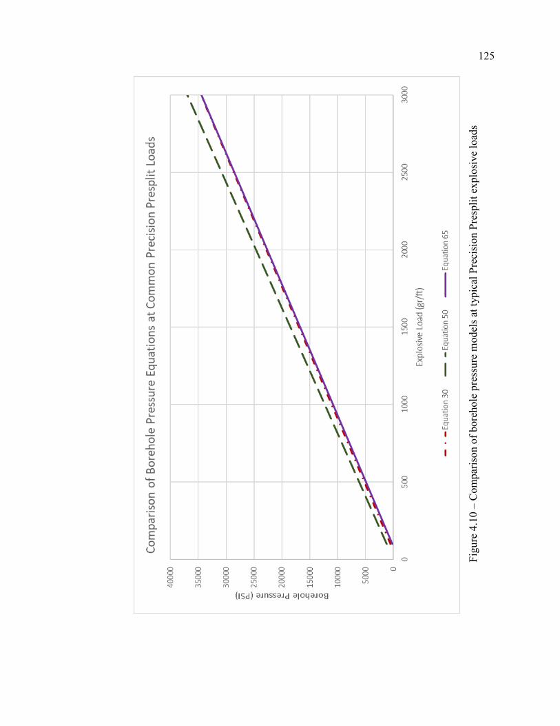
125
Figu
re 4
.10
– C
ompa
rison
of b
oreh
ole
pres
sure
mod
els a
t typ
ical
Pre
cisi
on P
resp
lit e
xplo
sive
load
s
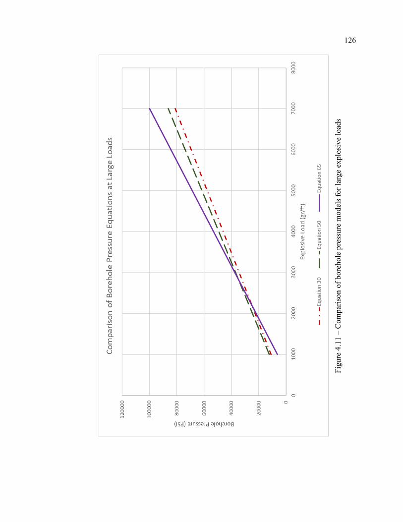
126
Figu
re 4
.11
– C
ompa
rison
of b
oreh
ole
pres
sure
mod
els f
or la
rge
expl
osiv
e lo
ads

127
4.5. BOTTOM CHARGE EFFECTS
A typical Precision Presplit load on a 24” spacing will utilize between 100 grains
per foot and 700 grains per foot of detonating cord depending on the rock type. The
typical loads at this spacing are shown in Table 4.16. As this spacing is expanded the
explosive load is increased to typically a maximum of 1500 grains per foot; as the
spacing is decreased the explosive load is decreased, with a minimum explosive load of
50 grains per foot. The typical borehole length that is used in industry is between 10
feet and 25 feet; with some Precision Presplit blasts having a borehole length of up to
50 feet. The reason the borehole length is typically kept short is that the drill deviation
becomes severe as the boreholes increase in length and blasters often state that longer
boreholes make it more difficult to presplit than shorter boreholes.
Table 4.16 – Typical explosive column load for various rock types
Rock Type Explosive Load through Borehole (ELc)
Granite 700 grains per foot
Limestone 500 grains per foot
Shale 300 grains per foot
Sandstone 250 grains per foot
Siltstone 100 grains per foot
The load which is brought throughout the entire borehole will be termed the
‘column load’ (ELc) as it is the load that is continuous throughout the entire powder
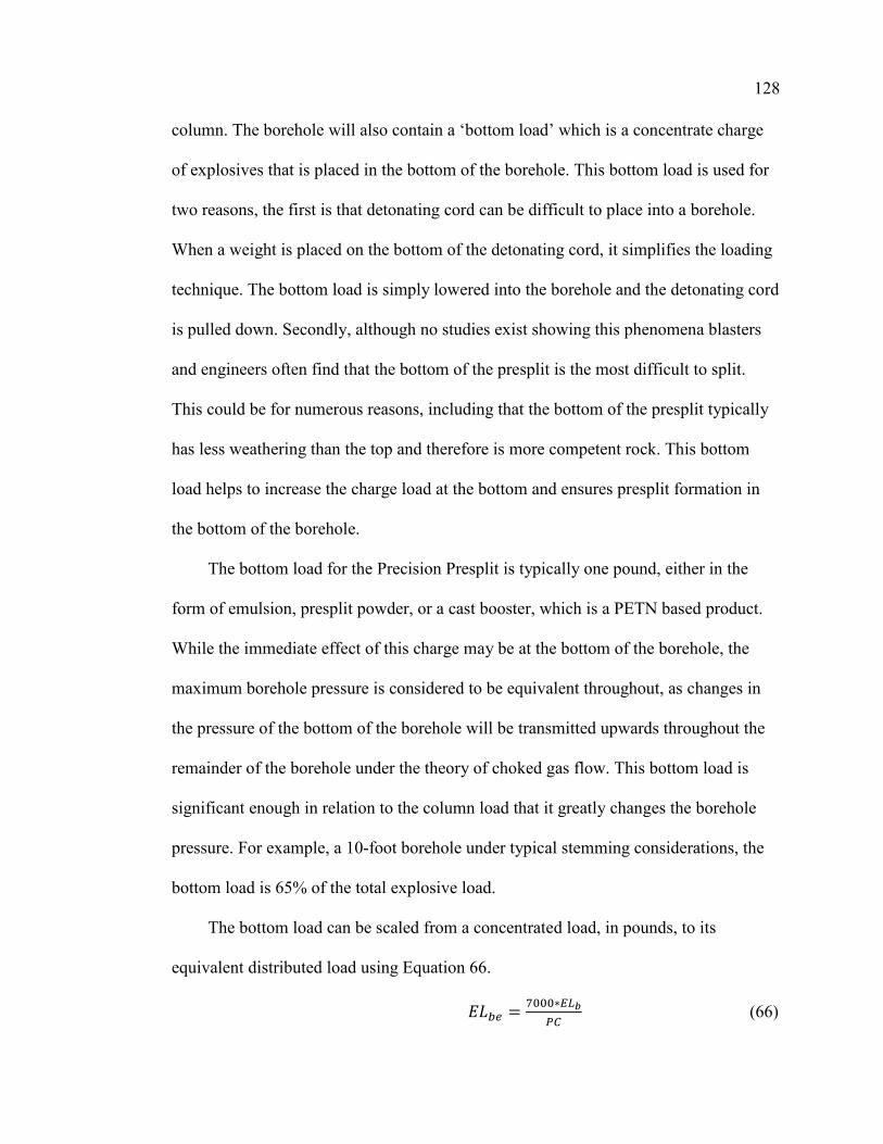
128
column. The borehole will also contain a ‘bottom load’ which is a concentrate charge
of explosives that is placed in the bottom of the borehole. This bottom load is used for
two reasons, the first is that detonating cord can be difficult to place into a borehole.
When a weight is placed on the bottom of the detonating cord, it simplifies the loading
technique. The bottom load is simply lowered into the borehole and the detonating cord
is pulled down. Secondly, although no studies exist showing this phenomena blasters
and engineers often find that the bottom of the presplit is the most difficult to split.
This could be for numerous reasons, including that the bottom of the presplit typically
has less weathering than the top and therefore is more competent rock. This bottom
load helps to increase the charge load at the bottom and ensures presplit formation in
the bottom of the borehole.
The bottom load for the Precision Presplit is typically one pound, either in the
form of emulsion, presplit powder, or a cast booster, which is a PETN based product.
While the immediate effect of this charge may be at the bottom of the borehole, the
maximum borehole pressure is considered to be equivalent throughout, as changes in
the pressure of the bottom of the borehole will be transmitted upwards throughout the
remainder of the borehole under the theory of choked gas flow. This bottom load is
significant enough in relation to the column load that it greatly changes the borehole
pressure. For example, a 10-foot borehole under typical stemming considerations, the
bottom load is 65% of the total explosive load.
The bottom load can be scaled from a concentrated load, in pounds, to its
equivalent distributed load using Equation 66.
𝐸𝐸𝐸𝐸𝑏𝑏𝑒𝑒 = 7000∗𝐸𝐸𝐸𝐸𝑏𝑏𝑃𝑃𝐶𝐶
(66)
129
where ELbe is the Equivalent Bottom Load in grains per foot, ELb is the bottom load in
pounds, and PC is the length of powder column in feet. The total explosive load in the
borehole is then the combination of the column load and the bottom load, which can be
calculated using Equation 67.
𝐸𝐸𝐸𝐸𝑒𝑒 = 𝐸𝐸𝐸𝐸𝑐𝑐 + 𝐸𝐸𝐸𝐸𝑏𝑏𝑒𝑒 (67)
where ELe is the Equivalent Explosive Load in grains per foot, ELc is the column load in
grains per foot, and ELbe is the equivalent bottom load in grains per foot. This equivalent
explosive load would be used to determine the borehole pressure in the previously
presented borehole pressure equations.
The current method of Precision Presplitting uses a set bottom load of one-pound
of explosive product. Under this case, the borehole pressure then varies based on the
length of the borehole. This can be modelled to show the differences in borehole pressure
based on borehole length and is shown in Figure 4.12. This chart shows that as the
borehole length exceeds 30 feet, the borehole pressure begins to reach a steady state and
the effects of the bottom load are not as significant. The 10-foot borehole has double the
borehole pressure of a 50-foot borehole. This would indicate that for boreholes which are
greater than 25 to 30 feet, the column load would need to be increased to increase the
overall borehole pressure.
The typical methods of Precision Presplitting have been analyzed for construction
blasting on lock and dam projects by past authors. These situations use the short benches
and bottom load considerations have not been previously analyzed. This indicates that the
bottom load for these short benches is a major source of pressure and cannot be ignored
in further analysis of the topic.
130
Figu
re 4
.12
– Bo
reho
le P
ress
ure
as a
func
tion
of b
oreh
ole
leng
th sh
owin
g th
e ef
fect
s of t
he b
otto
m lo
ad w
ith a
co
lum
n lo
ad o
f 500
gra
ins p
er fo
ot

131
4.6. PRESSURE OF A TYPICAL PRECISION PRESPLIT
The borehole pressure for a Precision Presplit blast can then be found through the
applications of Equations 65, 66, and 67. These equations will incorporate the bottom
load as a function of the borehole length and the column load. For example, a common
Precision Presplit blast in many U.S. Army Corp of Engineer’s projects is to use a
borehole length of ten-feet at the bottom of a project. Assuming that the rock is limestone
the column load is 500 grains per foot, the bottom load is one-pound, and the blaster
plans to use 2.5-feet of stemming, which results in a powder column of 7.5-feet, Equation
66 then yields:
𝐸𝐸𝐸𝐸𝑏𝑏𝑒𝑒 =7000 ∗ 1
7.5= 933.3 𝑔𝑔𝑔𝑔𝑔𝑔𝑔𝑔𝜌𝜌𝑠𝑠 𝑝𝑝𝑒𝑒𝑔𝑔 𝑓𝑓𝑓𝑓𝑓𝑓𝑓𝑓
The equivalent bottom load of 933.3 grains per foot is then incorporated into
Equation 67, with a column load of 500 grains per foot, which yields
𝐸𝐸𝐸𝐸𝑒𝑒 = 500𝑔𝑔𝑔𝑔𝑓𝑓𝑓𝑓
+ 933𝑔𝑔𝑔𝑔𝑓𝑓𝑓𝑓
= 1,433𝑔𝑔𝑔𝑔𝑓𝑓𝑓𝑓
The equivalent explosive load is then used in Equation 65 to get the borehole
pressure which yields
𝑃𝑃𝑔𝑔 = 0.00076 ∗ 14332 + 9.5 ∗ 1433 = 15,174 𝑃𝑃𝑆𝑆𝐼𝐼
The borehole pressure is then 15,174 psi for this example. This process can then
be completed for any changes in the explosive load. If changes are to be made to the
borehole diameter then Equation 63 can be used. With major changes to other variables
such as the explosive type then the full Thermodynamic Model can be applied.
132
5. HOOP STRESS MODEL FOR BLASTING
5.1. DEVELOPMENT OF HOOP STRESS MODEL
The borehole pressure for various situations of blasting can now be determined
from the application of either the Empirical Model, The Detonation Pressure Model, or
the Thermodynamic Model. This is beneficial but does not give any insight into how the
rock is actually breaking in a Precision Presplit. In order to determine how the rock is
breaking, the magnitude of the stress field must be computed. The breakage process for a
Precision Presplit breaking under the mechanisms of a Hoop Stress field has been
previously discussed and the modelling method of a thick-walled pressure vessel has
been presented in Equation 20. Equation 20 has been modified to include blasting
specific terminology in Equation 68.
𝜎𝜎𝑐𝑐 = �𝑃𝑃𝑔𝑔𝑑𝑑ℎ2−𝑝𝑝𝑜𝑜𝑆𝑆2
𝑆𝑆2−𝑑𝑑ℎ2 � − �𝑑𝑑ℎ
2𝑆𝑆2�𝑝𝑝𝑜𝑜−𝑃𝑃𝑔𝑔�𝑑𝑑2�𝑆𝑆2−𝑑𝑑ℎ
2�� (68)
where σc is the Circumferential Hoop Stress in psi, Pg is the borehole pressure in psi, dh is
the diameter of the borehole in inches, po is the pre-existing rock stress, S is the spacing
in inches, and d is the distance away from the center of the borehole in inches.
In a majority of situations for surface blasting where some excavation has already
taken place, it will be assumed that the pre-existing rock stress is very small compared to
the borehole pressure. This would treat the pre-existing rock stress as zero. This yields
Equation 69.
𝜎𝜎𝑐𝑐 = � 𝑃𝑃𝑔𝑔𝑑𝑑ℎ2
𝑆𝑆2−𝑑𝑑ℎ2� + � 𝑑𝑑ℎ
2𝑆𝑆2𝑃𝑃𝑔𝑔𝑑𝑑2�𝑆𝑆2−𝑑𝑑ℎ
2�� (69)
133
The distance that the stress field is from the borehole, d, will be defined as a
function of the spacing as shown in Equation 70.
𝐴𝐴 = 𝑑𝑑𝑆𝑆 (70)
where A is the distance constant, d is the distance away from the borehole in inches, and
S is the spacing in inches. The constant ‘A’ will vary between a value of 𝑑𝑑ℎ2𝑆𝑆
and 1.
Equation 70 will be substituted into Equation 69, which yields Equation 71.
𝜎𝜎𝑐𝑐 = � 𝑃𝑃𝑔𝑔𝑑𝑑ℎ2
𝑆𝑆2−𝑑𝑑ℎ2� + � 𝑑𝑑ℎ
2𝑆𝑆2𝑃𝑃𝑔𝑔𝐴𝐴2𝑆𝑆2�𝑆𝑆2−𝑑𝑑ℎ
2�� (71)
Simplification of Equation 71 yields Equation 72.
𝜎𝜎𝑐𝑐 = 𝑃𝑃𝑔𝑔𝑑𝑑ℎ2�𝐴𝐴2+1�
𝐴𝐴2�𝑆𝑆2−𝑑𝑑ℎ2�
(72)
where σc is the Circumferential Hoop Stress in psi, Pg is the borehole pressure in psi, dh is
the diameter of the borehole in inches, S is the spacing in inches, and A is the distance
constant as defined in Equation 70. Equation 72 can now be utilized to calculate the
magnitude of the Hoop Stress field at any distance in between two boreholes based on the
explosive pressure.
Precision Presplitting functions with every borehole containing an explosive load.
It will then be assumed that each borehole would cause a fracture to form to halfway
between the boreholes, or half the spacing. This area results in an ‘A’ value of ½ which
will be called the maximum split distance. In situations where the second borehole is not
loaded, the A value will would reach a value of 1.0 to indicate that the fracture from the
borehole would need to split the entire spacing distance, resulting in an increase to the
explosive load.
134
The fracture formation of the presplit starts at the borehole wall and is modelled
by a distance constant (A) of 𝑑𝑑ℎ2𝑆𝑆
. Figure 5.1 shows that near the borehole wall the pressure
is extremely large. As the distance away from the borehole increases, the magnitude of
the hoop stress is rapidly reduced and is approximately 5% halfway between the
boreholes when compared to what it is at the borehole wall. The hoop stress field at the
adjacent borehole is less than 2% than the stress next to the borehole that fires.
The stress produced on the adjacent borehole produces a circumferential loading
profile which is similar to what is found from overburden stresses on a mine opening.
This creates a stress field around the borehole causing the sides of the borehole which are
oriented towards the presplit line to have a stress of minus sigma (-σ) and at a 90° and
270° direction of the borehole to be in a stress state of three sigma (3σ). This places the
borehole into differential loading, this differential loading causes the presplit to align
between boreholes and prevents additional fracturing which can cause backbreak.
Furthermore, each borehole typically has one borehole being detonated on each
side of the blast, which causes double the circumferential loading. This would signify that
the borehole has 12% of the stress found at the borehole wall, which is acting in
compression to prevent overbreak at 90° and 270° around the borehole, and 4% of the
total pressure, which helps to align the presplit fracture between boreholes.
This results in a circumferential loading of 16% around the borehole, with 12% of
the stress at the borehole stopping overbreak from occurring and 4% of the stress causing
a fracture to form between boreholes. This circumferential loading helps to explain why
the presplit fracture aligns between boreholes and minimizes the overbreak past the
intended presplit line. This loading is further discussed in Appendix D.

135
Assuming both boreholes are loaded with explosives the maximum split distance
is defined as halfway between the boreholes, which produces a distance constant (A) of
0.5. Holding the borehole diameter and the explosive load as constants, the hoop stress
field can be analyzed based on the borehole spacing. Figure 5.2 shows this relationship,
of the hoop stress as a function of spacing. The hoop stress field is a function of the
square of the distances, which is the same result that was found from empirical work.
The effect of the borehole diameter can also be analyzed from the Hoop Stress
Equation. The borehole diameter influences both the magnitude of the Hoop Stress field
and the borehole pressure. The borehole pressure can be modeled from Equation 63 to
determine the effects of borehole diameter and this borehole pressure can then be applied
in Equation 72. The maximum split distance will again be assumed to be halfway
between boreholes to observe a distance constant (A) of 0.5. The explosive load and
spacing are then kept constant and the series of equations will only be a function of the
borehole diameter.
This analysis proves a phenomenon which has been discussed in the blasting
industry. Experts in the blasting industry often state that the diameter of the borehole did
not matter, if the explosive load is properly matched to the spacing of the boreholes
(Konya & Walter, 1990). This confused many in the industry as it was believed that this
changed the internal borehole pressure. This is often used by proponents of the
shockwave breakage mechanisms as a proof against the gas pressure in the borehole
causing the presplit. It is claimed that if the borehole pressure is reduced and no effect on
the presplit occurs then it must be the shockwave, which does not change based on the
borehole diameter, which causes the presplit to form.

136
However, as the borehole diameter is increased, with spacing remaining constant,
the web of rock between the boreholes decreases. The decrease in the total web of rock
from an increasing borehole diameter has a larger impact on the hoop stress field than the
decrease in the reduction of the borehole pressure from the increased diameter. This
results in a minimal change in the rock stress when the borehole diameter is less than
25% of the spacing, and an increase in the stress field when the borehole diameter is
larger than 25% of the spacing. This has been shown in Figure 5.3, which shows the
magnitude of the hoop stress field halfway between the boreholes for variations in the
borehole diameter.
This state then when the spacing is held constant and the borehole diameter is
increased, the explosive load can remain the same to still cause the presplit to form. This
has been found in the field for project which utilize Precision Presplitting. For example, if
the spacing is held constant at 24 inches between boreholes, it does not matter if the
borehole is 3” or 3.5” in diameter, the explosive load would be the same to generate the
presplit. This is due to the decreased distance the explosive must split between boreholes.
However, in a majority of situations when the borehole diameter is increased,
such as in the mining industry which can use up to 10-inch diameter boreholes for
presplitting, the spacing is also increased. In this situation, where both the spacing and
borehole diameter are increased, changes are visible to the Hoop Stress Field. This
situation would not follow this relationship as the web of rock between holes increases.

137
Figu
re 5
.1 –
Hoo
p st
ress
fiel
d as
a fu
nctio
n of
the
dist
ance
con
stan
t (A
)

138
Figu
re 5
.2 –
The
eff
ect o
f spa
cing
bet
wee
n bo
reho
les o
n th
e ho
op st
ress
fiel
d m
agni
tude

139
Figu
re 5
.3 –
Var
iatio
ns o
f hoo
p st
ress
mag
nitu
de to
bor
ehol
e di
amet
er h
alfw
ay b
etw
een
the
bore
hole
s
140
5.2. SIMPLIFICATION OF HOOP STRESS MODEL
The combination of Equations 63, 64, and 72 results in Equation 73 which can be
used to determine the Hoop Stress Field from a Precision Presplit Blast from the
equivalent explosive load in grains per foot.
𝜎𝜎𝑐𝑐 = �0.00684∗𝐸𝐸𝐸𝐸𝑒𝑒2+85.5∗𝐸𝐸𝐸𝐸𝑒𝑒��𝐴𝐴2+1�𝐴𝐴2�𝑆𝑆2− 𝑑𝑑ℎ
2� (73)
where σc is the magnitude of the hoop stress field in psi, ELe is the equivalent explosive
load in grains per foot, A is the distance constant, S is the spacing in inches, and dh is the
borehole diameter in inches.
Equation 73 can be further simplified to develop a general equation for the typical
case of a Precision Presplit. In this case the spacing is 24 inches and the borehole
diameter is three inches. Furthermore, the maximum split distance is assumed to be
halfway between the boreholes. This implies that each borehole will require enough
explosive load to cause the presplit formation to halfway between boreholes. This would
set a distance constant (A) value of 0.5. These assumptions for Equation 73 result in
Equation 74, which is a simplified equation for the determination of the Hoop Stress from
the explosive load in a Precision Presplit.
𝜎𝜎𝑐𝑐 = 0.00006 ∗ 𝐸𝐸𝐸𝐸𝑒𝑒2 + 0.76𝐸𝐸𝐸𝐸𝑒𝑒 (74)
where σc is the circumferential hoop stress in psi and ELe is the equivalent explosive load
in grains per foot.
The equivalent explosive load must generate enough stress to exceed the tensile
strength of the rock mass in order to develop the presplit. The Brazilian Tensile Strength
will be considered the tensile strength of the rock and denoted as σB. The circumferential
hoop stress in Equation 74 is then equal to the tensile strength for the explosive load,
141
which will cause a presplit to form. Equation 74 can then be solved through the quadratic
formula and simplified to Equation 75, which can be used to determine the equivalent
explosive load necessary to cause a presplit to form based on the rock’s tensile strength.
𝐸𝐸𝐸𝐸𝑒𝑒 = −6300 + 130�2,400 + 𝜎𝜎𝐵𝐵 (75)
where ELe is the equivalent explosive load in grains per foot and σB is the Brazilian
Tensile Strength of the rock in psi. This gives engineers a new tool to determine the
explosive load for a Precision Presplit blast which has a 24” spacing between boreholes.
5.3. HOOP STRESS OF A PRECISION PRESPLIT BLAST
Previously published data has shown what average values for the explosive load
are based on the rock type, which are provided in Table 5.1. These explosive loads are
commonly used field loads for a 10-foot to 15-foot bench with a one-pound bottom load.
The previous models can then be used in accordance with what is applied daily in the
field to determine if the calculated magnitude of the hoop stress matches the application
of this technology in the real world. This can be viewed as validation of this
methodology.
Equations 66 and 67 can be used to find the equivalent explosive load for these
situations assuming a 10-foot bench, which is commonly used in the final excavation of
many large construction projects. The bottom explosive load for all these situations
would then be equal to 700 grains per foot (ELB).
The equivalent explosive load (ELe) is then shown for these rock types in Table
5.2 which includes both the equivalent distributed bottom charge and the column charge.
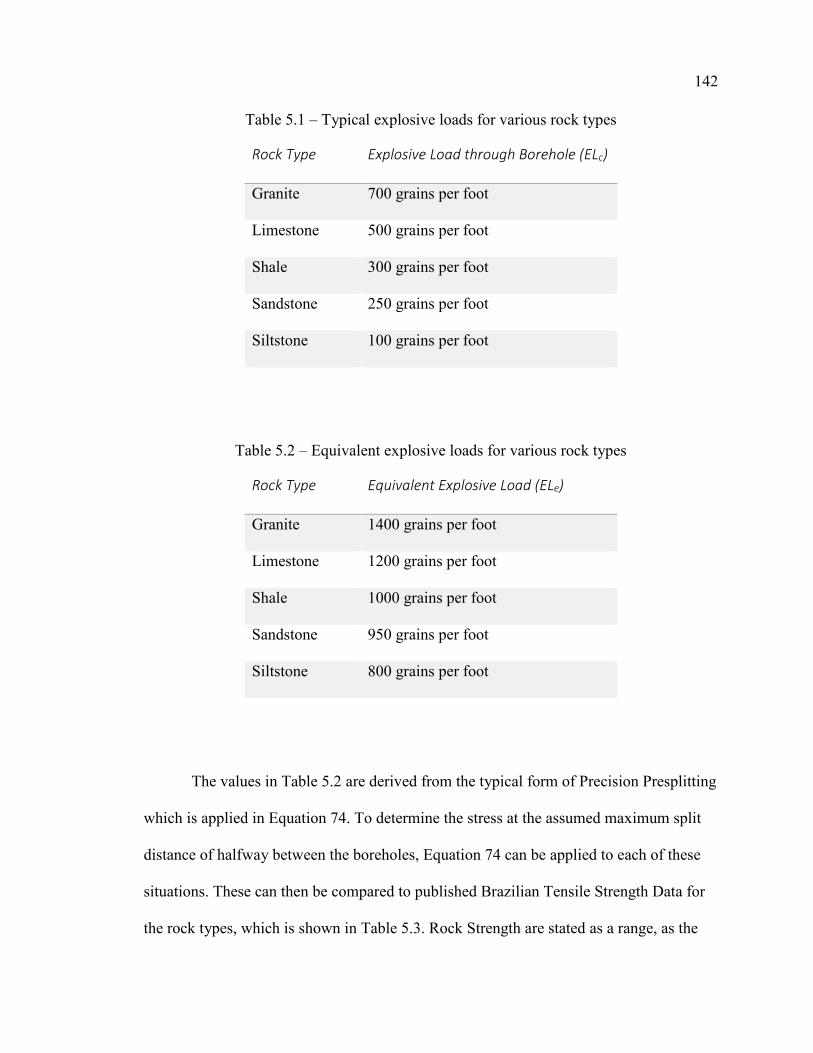
142
Table 5.1 – Typical explosive loads for various rock types
Rock Type Explosive Load through Borehole (ELc)
Granite 700 grains per foot
Limestone 500 grains per foot
Shale 300 grains per foot
Sandstone 250 grains per foot
Siltstone 100 grains per foot
Table 5.2 – Equivalent explosive loads for various rock types
Rock Type Equivalent Explosive Load (ELe)
Granite 1400 grains per foot
Limestone 1200 grains per foot
Shale 1000 grains per foot
Sandstone 950 grains per foot
Siltstone 800 grains per foot
The values in Table 5.2 are derived from the typical form of Precision Presplitting
which is applied in Equation 74. To determine the stress at the assumed maximum split
distance of halfway between the boreholes, Equation 74 can be applied to each of these
situations. These can then be compared to published Brazilian Tensile Strength Data for
the rock types, which is shown in Table 5.3. Rock Strength are stated as a range, as the

143
strength widely varies based on weathering and structure and are compiled from various
sources for what may be commonly observed in the field (Li & Wong, 2012; University
of Texas, 2019; Hoek, Marinos, & Marinos).
Table 5.3 – Comparison of hoop stress at maximum split distance to rock tensile strength
Rock Type Hoop Stress at Maximum Split Distance Tensile Strength
Granite 1182 psi 1000 psi to 2500 psi
Limestone 998 psi 725 psi to 1500 psi
Shale 820 psi 300 psi to 1000 psi
Sandstone 776 psi 575 psi to 2500 psi
Siltstone 646 psi 400 psi
Table 5.3 clearly shows that in all situations the Hoop Stress Field at the assumed
maximum split distance, which is halfway between the boreholes, is greater than the
lower ranges of the measured Brazilian Tensile Strength for various rocks. It is important
to note that the presplit fracture will form at the borehole wall and then this fracture will
travel away from the borehole towards the second borehole. In order for the presplit to
fully form, the fracture must extend to at least halfway between the boreholes.
Furthermore, the tensile strength which is reported here is oftentimes much
greater than what is actually observed in the field. It is well known in the field of rock
mechanics that due to limitations of testing, based on sample screening and selection, the
‘best’ samples are chosen meaning those with the highest strength. The strength of the

144
rock mass is then typically weaker than the mass of the matrix due to structure. It has
been documented that this does have large effects on the ability to presplit the material
(Worsey P. , 1981). Additionally, rock which is typically being blasted is near the surface
and exhibits large amounts of weathering, which leads to a large decrease in strength. For
these reasons it is likely that the rock which is being presplit will typically fall into the
lower end of the tensile strength ranges shown in Table 5.3.
The hoop stress field is not only applied at the maximum split distance but can be
analyzed throughout the entire region of the spacing. The fracture will start at the wall of
the borehole and move towards the maximum split distance. Figure 5.4 shows the hoop
stress near the borehole from field loading conditions. Near the borehole the stress field is
very large and is typically over 10,000 psi. As the distance from the borehole increases
the magnitude of the hoop stress drops rapidly. Figure 5.5 shows the hoop stress field for
the various rock types presented, from field loading conditions, as the distance is
increased, and the stress drops below 2,000 psi. The presplit will form until the
magnitude of the hoop stress field is less than the rock’s tensile strength.
At this point, the formation of the presplit may still continue, as the fracture
network will be filled with the explosive gases and the crack may be driven under gas-
driven fracture growth. Under this mechanism the gas pressure would continue driving
the fractures if the pressure is great enough after accounting for the increased volume. If
the pressure is not great enough then the gas will vent to the surface. These details are
beyond the purview of this dissertation and any effects of gas driven cracks are
considered minimal.

145
Figu
re 5
.4 –
Mag
nitu
de o
f hoo
p st
ress
fiel
d ne
ar th
e bo
reho
le
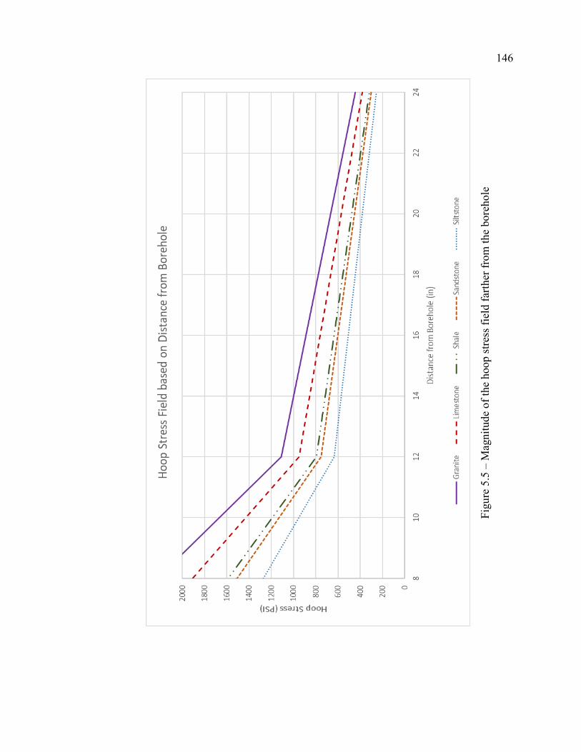
146
Figu
re 5
.5 –
Mag
nitu
de o
f the
hoo
p st
ress
fiel
d fa
rther
from
the
bore
hole
147
6. MAGNITUDE OF THE SHOCKWAVE FROM PRESPLITTING
6.1. SHOCKWAVE MECHANICS
A full analysis of shockwave mechanics is beyond the purview of this dissertation
and many texts treat the fundamental principles of shockwave motion and attenuation
(Cooper, 1996). However, for the purposes of a full analysis of the mechanics of a
presplit, the shockwave from precision presplitting will be calculated using impedance
mismatch. This will answer the question of what the rock may receive in terms of
shockwave pressures at the borehole wall.
To complete this analysis the starting conditions must be fully documented, which
include critical assumptions. It is important to understand the concept of failure of
structures in a dynamic situation, for this situation the rock will be assumed to break in
tension and since it is from a blast it will break dynamically. When a rock is loaded
dynamically, meaning that the time of loading is short, it has a much higher strength than
a slower loading, as it cannot respond to the stress and strain to the correct degree for
breakage to occur. The faster the loading the higher the strength and today there is no
data that can show the strength of rock under loading mechanics such as that from a
shockwave. The closest tensile strength which may be considered comes from Brazilian
disk tests which are shown in Table 5.3. The minimum Brazilian tensile strength for
granites is 1000 psi and will be the tensile strength used for this analysis.
Additionally, it will be assumed that for both situations the explosive is decoupled
and not in contact with the rock wall. The Precision Presplit will utilize 700 grains per
foot (150 grams per meter) of detonating cord as the explosive charge which has a

148
velocity of detonation (VOD) of 21,500 ft/s (6,500 m/s) and a density of 1.5 g/cc
(approximated from detonation rate, likely an overestimate leading to higher shock
pressures than actually observed in the field). The spacing for these boreholes in a
Precision Presplit will be considered to be 2 feet. This will not account for non-ideal
detonation of these explosives or attenuation of the shockwave through the rock mass.
It is important to note that the pressure of the shockwave from the explosive does
not change based on the explosive weight. The shockwave magnitude is solely a function
of the velocity of detonation and the density (Cooper, 1996; Lusk & Silva, 2018).
Therefore, if a larger charge is used in a borehole, such as the bottom charge in a
Precision Presplit, the magnitude of the shockwave would still be the same and mass
difference do not need to be considered.
6.2. SHOCKWAVE MAGNITUDE FOR A PRECISION PRESPLIT
For the case of Precision Presplitting, the detonation pressure will need to be
determined through a simplified CJ pressure equation, which is presented in Equation 6.
When utilizing this for detonation cord, assuming the density of the PETN is 1.5 g/cc and
the VOD is 6.5 km/s, the detonation pressure would be 2,297,000 psi.
𝑃𝑃𝐶𝐶𝐶𝐶 =1.5 𝑔𝑔
𝑐𝑐𝑐𝑐 ∗ 6.5 𝜌𝜌𝑘𝑘𝑠𝑠2
4= 15.84 𝑠𝑠𝑃𝑃𝑔𝑔 = 2,297,000 𝑝𝑝𝑠𝑠𝑔𝑔
The impedance of the detonating cord is 9,750,000. The transmission of the
shockwave from the detonating cord to the air is then 0.00016, or 0.016% of the
shockwave will be transmitted from the explosive into the air. The transmission of the
shockwave from the air to the rock is then 0.00009, or 0.009% of the shockwave is

149
transmitted from the air into the rock. The total transmission from the explosive to the
rock would then be 0.000000014 or 0.0000014%.
With 2,291,000 psi of shockwave pressure developed from the explosive, the total
pressure to reach the borehole wall would be 0.033 psi, which is well below the required
minimum to break a granite under tensile loading of 1000 psi. From this simple analysis
the shockwave cannot cause tensile breakage at the borehole wall, yet alone when
reduced to account for the shockwaves decay (attenuation) through the rock mass.
The total shockwave pressures at the borehole walls from both of these methods
are extremely small compared to the rock’s tensile strength when only considering basic
impedance mismatch concepts. If the analysis was completed using more advanced
methods with the incorporation of additional field values the result would conclude
smaller shockwave pressure values than what is calculated here. Furthermore, the
shockwave is a unique wave which must be of a very large pressure to where it travels
faster than the speed of sound in the material. The magnitude of the shockwave by the
time it reaches the borehole wall is so low that it is unlikely a shockwave would be
readily formed in the rock mass, in direct comparison to a borehole which is bulk loaded
with explosives and has direct contact between the explosive and the rock. For the case of
Precision Presplitting, the pressure of the shockwave is extremely low and likely
unobservable in the rock mass, and as such would be considered to have no effect in the
development of the presplit.
The magnitude of the shockwave is too low to cause any presplit fracture to form.
This alone completely refutes any effects of the shockwave on the formation of the
presplit. Further proof of the inapplicability of the shockwave to be used in presplit

150
fundamentals would be the application of propellant based explosives causing presplit
formation, the actual time of the formation of the presplit compared to the time of arrival
of the shockwave, and the inability to accurate time the blastholes to fire to cause
shockwave collisions.
151
7. RESULTS AND DISCUSSION
The detonation of an explosive which is confined in a borehole results in two
separate events which influence the breakage of the surrounding rock mass. The first of
these events is the generation of the shockwave, which is a rapidly moving high pressure
wave. The second event is the pressurization of the borehole as the high-temperature
gases expand and put stress on the walls of the borehole.
A Precision Presplit is a specialty method of blasting which uses extremely light
loads that are decoupled resulting in them not being in contact with the walls. This leads
to large losses in the pressure of the shockwave, as it must move through the explosive
and into the air then through the air and into the rock. Furthermore, the shockwave
quickly attenuates, or decreases in pressure, as it moves through the rock. The shockwave
is modelled through a simplified impedance mismatch approach to determine its stress at
various points in the rock.
The gas pressure from the Precision Presplit quickly expands to fill the borehole
and results in the generation of a hoop stress field in the rock. The borehole pressure has
been modelled from three separate approaches which all show excellent accuracy to
experimentation. A model is presented in this dissertation to determine the magnitude of
the hoop stress field from the borehole pressure. This allows for the generation of the
magnitude of both the shockwave stress and hoop stress at a distance of one borehole
diameter away from the borehole wall, and this is shown in Table 7.1.
Table 7.1 clearly shows that the hoop stress field is extremely large near the
borehole and exceeds the Brazilian Tensile Strength of the rock in all situations. The
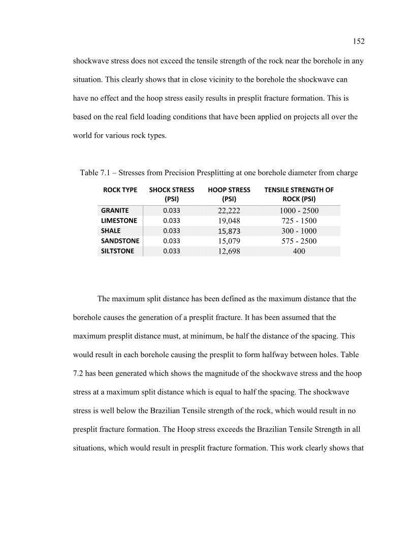
152
shockwave stress does not exceed the tensile strength of the rock near the borehole in any
situation. This clearly shows that in close vicinity to the borehole the shockwave can
have no effect and the hoop stress easily results in presplit fracture formation. This is
based on the real field loading conditions that have been applied on projects all over the
world for various rock types.
Table 7.1 – Stresses from Precision Presplitting at one borehole diameter from charge
ROCK TYPE SHOCK STRESS (PSI)
HOOP STRESS (PSI)
TENSILE STRENGTH OF ROCK (PSI)
GRANITE 0.033 22,222 1000 - 2500 LIMESTONE 0.033 19,048 725 - 1500 SHALE 0.033 15,873 300 - 1000 SANDSTONE 0.033 15,079 575 - 2500 SILTSTONE 0.033 12,698 400
The maximum split distance has been defined as the maximum distance that the
borehole causes the generation of a presplit fracture. It has been assumed that the
maximum presplit distance must, at minimum, be half the distance of the spacing. This
would result in each borehole causing the presplit to form halfway between holes. Table
7.2 has been generated which shows the magnitude of the shockwave stress and the hoop
stress at a maximum split distance which is equal to half the spacing. The shockwave
stress is well below the Brazilian Tensile strength of the rock, which would result in no
presplit fracture formation. The Hoop stress exceeds the Brazilian Tensile Strength in all
situations, which would result in presplit fracture formation. This work clearly shows that

153
the shockwave has no effect on the presplit fracture formation, while the hoop stress field
has the proper magnitude to be the major mechanism in the presplit fracture formation.
Table 7.2 – Stresses from Precision Presplitting at maximum split distance
ROCK TYPE SHOCK STRESS (PSI)
HOOP STRESS (PSI)
TENSILE STRENGTH OF ROCK (PSI)
GRANITE 0.002 1182 1000 - 2500 LIMESTONE 0.002 998 725 - 1500 SHALE 0.002 820 300 - 1000 SANDSTONE 0.002 776 575 - 2500 SILTSTONE 0.002 646 400
The development of Tables 7.1 and 7.2 is based on the use of actual field data for
the typical explosive loads which are used, in general, with various rock types. The fact
that the hoop stress field exceeds the tensile strength of the rock at a distance of half the
spacing is a remarkable finding. A theory is not applicable unless it provides the
background and the reason why something occurs in the field. The shockwave theory has
never been shown to be applicable to the field conditions which are used in the real
world. The hoop stress theory has proven to show the reason behind the field conditions.
This theory would also hold with other common methods of presplitting. The
hoop stress field is the only stress which is exerted in a propellant presplit blast. A
traditional presplit blast also has large shockwave pressure losses due to impedance
mismatches and would have larger hoop stresses than reported here. An airdeck presplit,
which has only the bottom of the hole filled with explosive, would also have minimal
shockwaves near the top of the hole but would have large hoop stress fields between

154
holes after the borehole has been pressurized fully. This hoop stress theory does not only
hold for the case of Precision Presplitting, but can accurately define the stress fields
around all the different types of commonly used presplit methods. This research then
shows that the shockwave has no effect in any presplit blast and the hoop stress is the
dominant breakage mechanic when a decoupled charge is used.

155
8. CONCLUSIONS
This work has shown that modelling a Precision Presplit blast as a function of
hoop stresses, similar to that of thick-walled pressure vessel, is an accurate method to
determine the stresses generated in a presplit blast. This work clearly shows that the
shock wave has no effect on the formation of a presplit when using Precision Presplitting
and the hoop stress field generated as a result of borehole gas pressurization is the major
mechanism which leads to the formation of the presplit. The application of the hoop
stress theory shows that the magnitude of the stress is available to cause the presplit to
form from typical field conditions.
This work has taken empirical and field data and provided the basis for how a
Precision Presplit actually works in the field and has theoretically proven many aspects of
presplitting, which have been discussed in the field for decades. These include showing
proof for why changing the borehole diameter does not require changes to the explosive
load, the disproof of split factor design of presplits and shows why split factor does not
work for design, and the proof of why delays can be used between presplit holes without
degradation of the presplit.
This work has shown that the presplit parameters can be correlated and designed
based on the Young’s Modulus of the rock and the Brazilian Tensile Strength. This
research has also shown that Precision Presplitting uses small borehole pressures to
generate large hoop stresses, based on the close spacing. This explains why geologic
structure affects a Precision Presplit less than a traditional presplit or other method of
overbreak.
156
APPENDIX A.
CALCULATIONS OF BOREHOLE PRESSURE FOR PETN

157
Appendix A contains various runs of the Thermodynamic Borehole Pressure
Model, for the charge loads which were used in experimentation completed by Otuonye.
The work completed is in the same manner as the work shown in Section 4.3 of this
dissertation to validate the Thermodynamic Model from field tested data and determine
the total error of the Thermodynamic Model.
The starting variables for each charge size are shown, as well as calculations for
the reduced temperature, which do not change as the explosive used is always PETN.
These models were then completed with two to three iterations of the reduced pressure
and application of the compressibility curves to arrive at a final calculated borehole
pressure.

158
R = 0.08206 liter atm / mole K Product mole fraction Crit Te Tr Tr FracT = 4900 K H2O 0.363 647 7.573 2.749V = 0.257 L N2 0.182 126 38.889 7.078
ng = 0.0348 mol/gm CO2 0.273 304 16.118 4.400weight = 10 grams CO 0.182 133 36.842 6.705
n= 0.348 mol Tr = 20.933
P = (ZnRT)/VP = 544.47 Z (atm)P = 8004 Z (psi)
Assume P = 8000 PSI
Product mole fraction Press (Pc) Prod (Pr) Pr (Frac)H2O 0.363 3205 2.496 0.906N2 0.182 493 16.227 2.953CO2 0.273 1072 7.463 2.037CO 0.182 507 15.779 2.872
Pr = 8.769
Compressibility CurveTr 21Pr 8.77
Z = 1.04
P = 8323.85272
Assume P = 8325 PSI
Product mole fraction Press (Pc) Prod (Pr) Pr (Frac)H2O 0.363 3205 2.598 0.943N2 0.182 493 16.886 3.073CO2 0.273 1072 7.766 2.120CO 0.182 507 16.420 2.988
Pr = 9.125
Compressibility CurveTr 21Pr 9.12
Z = 1.05
P = 8403.889765
Assume P = 8400 PSI
Product mole fraction Press (Pc) Prod (Pr) Pr (Frac)H2O 0.363 3205 2.621 0.951N2 0.182 493 17.039 3.101CO2 0.273 1072 7.836 2.139CO 0.182 507 16.568 3.015
Pr = 9.207
Compressibility CurveTr 21Pr 9.21
Z = 1.05
P = 8403.889765Pressure = 8400 PSI
Temp of PETN 4900 K
Critical Temp
Critical Pressure

159
R = 0.08206 liter atm / mole K Product mole fraction Crit Te Tr Tr FracT = 4900 K H2O 0.363 647 7.573 2.749V = 0.257 L N2 0.182 126 38.889 7.078
ng = 0.0348 mol/gm CO2 0.273 304 16.118 4.400weight = 20 grams CO 0.182 133 36.842 6.705
n= 0.696 mol Tr = 20.933
P = (ZnRT)/VP = 1088.94 Z (atm)P = 16007 Z (psi)
Assume P = 17000 PSI
Product mole fraction Press (Pc) Prod (Pr) Pr (Frac)H2O 0.363 3205 5.304 1.925N2 0.182 493 34.483 6.276CO2 0.273 1072 15.858 4.329CO 0.182 507 33.531 6.103
Pr = 18.633
Compressibility CurveTr 21Pr 18.63
Z = 1.1
P = 17608.14998
Assume P = 17610 PSI
Product mole fraction Press (Pc) Prod (Pr) Pr (Frac)H2O 0.363 3205 5.495 1.995N2 0.182 493 35.720 6.501CO2 0.273 1072 16.427 4.485CO 0.182 507 34.734 6.322
Pr = 19.302
Compressibility CurveTr 21Pr 19.30
Z = 1.11
P = 17768.22408
Assume P = 17750 PSI
Product mole fraction Press (Pc) Prod (Pr) Pr (Frac)H2O 0.363 3205 5.538 2.010N2 0.182 493 36.004 6.553CO2 0.273 1072 16.558 4.520CO 0.182 507 35.010 6.372
Pr = 19.455
Compressibility CurveTr 21Pr 19.46
Z = 1.11
P = 17768.22408Pressure = 17750 PSI
Critical Temp
Critical Pressure

160
R = 0.08206 liter atm / mole K Product mole fraction Crit Te Tr Tr FracT = 4900 K H2O 0.363 647 7.573 2.749V = 0.257 L N2 0.182 126 38.889 7.078
ng = 0.0348 mol/gm CO2 0.273 304 16.118 4.400weight = 30 grams CO 0.182 133 36.842 6.705
n= 1.044 mol Tr = 20.933
P = (ZnRT)/VP = 1633.41 Z (atm)P = 24011 Z (psi)
Assume P = 26500 PSI
Product mole fraction Press (Pc) Prod (Pr) Pr (Frac)H2O 0.363 3205 8.268 3.001N2 0.182 493 53.753 9.783CO2 0.273 1072 24.720 6.749CO 0.182 507 52.268 9.513
Pr = 29.046
Compressibility CurveTr 21Pr 29.05
Z = 1.16
P = 27852.89179
Assume P = 27850 PSI
Product mole fraction Press (Pc) Prod (Pr) Pr (Frac)H2O 0.363 3205 8.690 3.154N2 0.182 493 56.491 10.281CO2 0.273 1072 25.979 7.092CO 0.182 507 54.931 9.997
Pr = 30.525
Compressibility CurveTr 21Pr 30.53
Z = 1.17
P = 28093.00293
Assume P = 28100 PSI
Product mole fraction Press (Pc) Prod (Pr) Pr (Frac)H2O 0.363 3205 8.768 3.183N2 0.182 493 56.998 10.374CO2 0.273 1072 26.213 7.156CO 0.182 507 55.424 10.087
Pr = 30.799
Compressibility CurveTr 21Pr 1.17
Z = 1.17
P = 28093.00293Pressure = 28100 PSI
Critical Temp
Critical Pressure

161
R = 0.08206 liter atm / mole K Product mole fraction Crit Te Tr Tr FracT = 4900 K H2O 0.363 647 7.573 2.749V = 0.257 L N2 0.182 126 38.889 7.078
ng = 0.0348 mol/gm CO2 0.273 304 16.118 4.400weight = 40 grams CO 0.182 133 36.842 6.705
n= 1.392 mol Tr = 20.933
P = (ZnRT)/VP = 2177.88 Z (atm)P = 32015 Z (psi)
Assume P = 38000 PSI
Product mole fraction Press (Pc) Prod (Pr) Pr (Frac)H2O 0.363 3205 11.856 4.304N2 0.182 493 77.079 14.028CO2 0.273 1072 35.448 9.677CO 0.182 507 74.951 13.641
Pr = 41.651
Compressibility CurveTr 21Pr 41.65
Z = 1.22
P = 39058.07815
Assume P = 39000 PSI
Product mole fraction Press (Pc) Prod (Pr) Pr (Frac)H2O 0.363 3205 12.168 4.417N2 0.182 493 79.108 14.398CO2 0.273 1072 36.381 9.932CO 0.182 507 76.923 14.000
Pr = 42.747
Compressibility CurveTr 21Pr 42.75
Z = 1.23
P = 39378.22633
Assume P = 39400 PSI
Product mole fraction Press (Pc) Prod (Pr) Pr (Frac)H2O 0.363 3205 12.293 4.462N2 0.182 493 79.919 14.545CO2 0.273 1072 36.754 10.034CO 0.182 507 77.712 14.144
Pr = 43.185
Compressibility CurveTr 21Pr 43.19
Z = 1.23
P = 39378.22633Pressure = 39400 PSI
Critical Temp
Critical Pressure
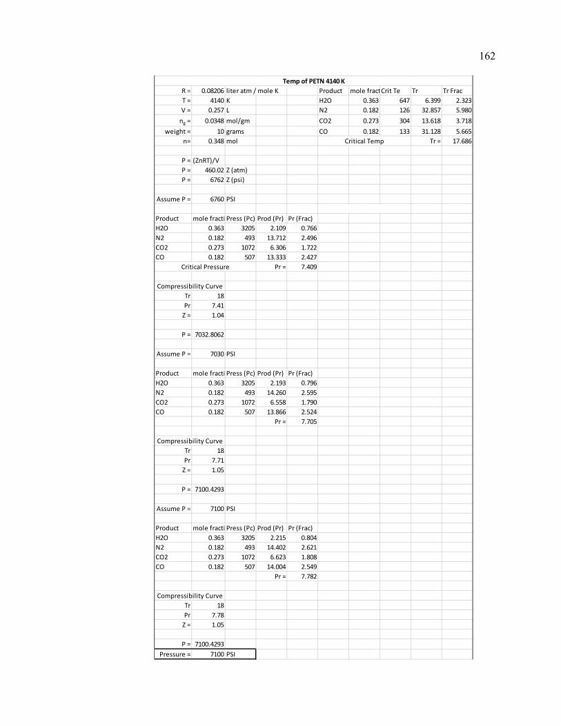
162
R = 0.08206 liter atm / mole K Product mole fractCrit Te Tr Tr FracT = 4140 K H2O 0.363 647 6.399 2.323V = 0.257 L N2 0.182 126 32.857 5.980
ng = 0.0348 mol/gm CO2 0.273 304 13.618 3.718weight = 10 grams CO 0.182 133 31.128 5.665
n= 0.348 mol Tr = 17.686
P = (ZnRT)/VP = 460.02 Z (atm)P = 6762 Z (psi)
Assume P = 6760 PSI
Product mole fracti Press (Pc) Prod (Pr) Pr (Frac)H2O 0.363 3205 2.109 0.766N2 0.182 493 13.712 2.496CO2 0.273 1072 6.306 1.722CO 0.182 507 13.333 2.427
Pr = 7.409
Tr 18Pr 7.41
Z = 1.04
P = 7032.8062
Assume P = 7030 PSI
Product mole fracti Press (Pc) Prod (Pr) Pr (Frac)H2O 0.363 3205 2.193 0.796N2 0.182 493 14.260 2.595CO2 0.273 1072 6.558 1.790CO 0.182 507 13.866 2.524
Pr = 7.705
Tr 18Pr 7.71
Z = 1.05
P = 7100.4293
Assume P = 7100 PSI
Product mole fracti Press (Pc) Prod (Pr) Pr (Frac)H2O 0.363 3205 2.215 0.804N2 0.182 493 14.402 2.621CO2 0.273 1072 6.623 1.808CO 0.182 507 14.004 2.549
Pr = 7.782
Tr 18Pr 7.78
Z = 1.05
P = 7100.4293Pressure = 7100 PSI
Compressibility Curve
Compressibility Curve
Compressibility Curve
Temp of PETN 4140 K
Critical Temp
Critical Pressure

163
R = 0.08206 liter atm / mole K Product mole fractCrit Te Tr Tr FracT = 4140 K H2O 0.363 647 6.399 2.323V = 0.257 L N2 0.182 126 32.857 5.980
ng = 0.0348 mol/gm CO2 0.273 304 13.618 3.718weight = 20 grams CO 0.182 133 31.128 5.665
n= 0.696 mol Critical Temp Tr = 17.686
P = (ZnRT)/VP = 920.04 Z (atm)P = 13525 Z (psi)
Assume P = 15000 PSI
Product mole fracti Press (Pc) Prod (Pr) Pr (Frac)H2O 0.363 3205 4.680 1.699N2 0.182 493 30.426 5.538CO2 0.273 1072 13.993 3.820CO 0.182 507 29.586 5.385
Pr = 16.441
Tr 18Pr 16.44
Z = 1.11
P = 15012.336
Assume P = 15000 PSI
Product mole fracti Press (Pc) Prod (Pr) Pr (Frac)H2O 0.363 3205 4.680 1.699N2 0.182 493 30.426 5.538CO2 0.273 1072 13.993 3.820CO 0.182 507 29.586 5.385
Pr = 16.441
Tr 18Pr 16.44
Z = 1.11
P = 15012.336
Assume P = 15000 PSI
Product mole fracti Press (Pc) Prod (Pr) Pr (Frac)H2O 0.363 3205 4.680 1.699N2 0.182 493 30.426 5.538CO2 0.273 1072 13.993 3.820CO 0.182 507 29.586 5.385
Pr = 16.441
Tr 18Pr 16.44
Z = 1.11
P = 15012.336Pressure = 15000 PSI
Critical Pressure
Compressibility Curve
Compressibility Curve
Compressibility Curve
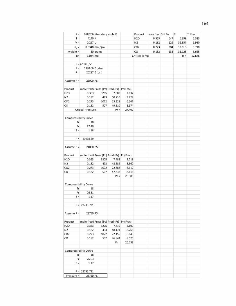
164
R = 0.08206 liter atm / mole K Product mole fractCrit Te Tr Tr FracT = 4140 K H2O 0.363 647 6.399 2.323V = 0.257 L N2 0.182 126 32.857 5.980
ng = 0.0348 mol/gm CO2 0.273 304 13.618 3.718weight = 30 grams CO 0.182 133 31.128 5.665
n= 1.044 mol Critical Temp Tr = 17.686
P = (ZnRT)/VP = 1380.06 Z (atm)P = 20287 Z (psi)
Assume P = 25000 PSI
Product mole fracti Press (Pc) Prod (Pr) Pr (Frac)H2O 0.363 3205 7.800 2.832N2 0.182 493 50.710 9.229CO2 0.273 1072 23.321 6.367CO 0.182 507 49.310 8.974
Pr = 27.402
Tr 18Pr 27.40
Z = 1.18
P = 23938.59
Assume P = 24000 PSI
Product mole fracti Press (Pc) Prod (Pr) Pr (Frac)H2O 0.363 3205 7.488 2.718N2 0.182 493 48.682 8.860CO2 0.273 1072 22.388 6.112CO 0.182 507 47.337 8.615
Pr = 26.306
Tr 18Pr 26.31
Z = 1.17
P = 23735.721
Assume P = 23750 PSI
Product mole fracti Press (Pc) Prod (Pr) Pr (Frac)H2O 0.363 3205 7.410 2.690N2 0.182 493 48.174 8.768CO2 0.273 1072 22.155 6.048CO 0.182 507 46.844 8.526
Pr = 26.032
Tr 18Pr 26.03
Z = 1.17
P = 23735.721Pressure = 23750 PSI
Critical Pressure
Compressibility Curve
Compressibility Curve
Compressibility Curve

165
R = 0.08206 liter atm / mole K Product mole fractCrit Te Tr Tr FracT = 4140 K H2O 0.363 647 6.399 2.323V = 0.257 L N2 0.182 126 32.857 5.980
ng = 0.0348 mol/gm CO2 0.273 304 13.618 3.718weight = 40 grams CO 0.182 133 31.128 5.665
n= 1.392 mol Critical Temp Tr = 17.686
P = (ZnRT)/VP = 1840.09 Z (atm)P = 27049 Z (psi)
Assume P = 33000 PSI
Product mole fracti Press (Pc) Prod (Pr) Pr (Frac)H2O 0.363 3205 10.296 3.738N2 0.182 493 66.937 12.183CO2 0.273 1072 30.784 8.404CO 0.182 507 65.089 11.846
Pr = 36.170
Tr 18Pr 36.17
Z = 1.24
P = 33541.076
Assume P = 33550 PSI
Product mole fracti Press (Pc) Prod (Pr) Pr (Frac)H2O 0.363 3205 10.468 3.800N2 0.182 493 68.053 12.386CO2 0.273 1072 31.297 8.544CO 0.182 507 66.174 12.044
Pr = 36.773
Tr 18Pr 36.77
Z = 1.25
P = 33811.568
Assume P = 33800 PSI
Product mole fracti Press (Pc) Prod (Pr) Pr (Frac)H2O 0.363 3205 10.546 3.828N2 0.182 493 68.560 12.478CO2 0.273 1072 31.530 8.608CO 0.182 507 66.667 12.133
Pr = 37.047
Tr 18Pr 37.05
Z = 1.25
P = 33811.568Pressure = 33800 PSI
Critical Pressure
Compressibility Curve
Compressibility Curve
Compressibility Curve

166
APPENDIX B.
PRECISION PRESPLIT BOREHOLE PRESSURE
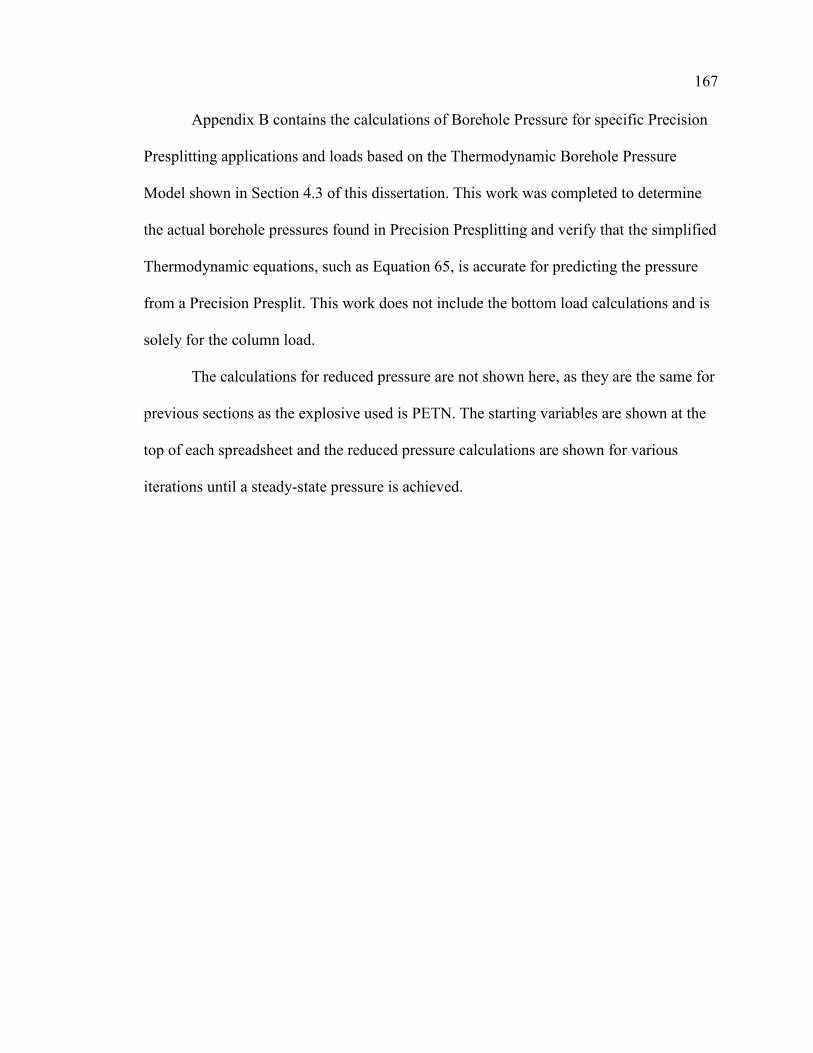
167
Appendix B contains the calculations of Borehole Pressure for specific Precision
Presplitting applications and loads based on the Thermodynamic Borehole Pressure
Model shown in Section 4.3 of this dissertation. This work was completed to determine
the actual borehole pressures found in Precision Presplitting and verify that the simplified
Thermodynamic equations, such as Equation 65, is accurate for predicting the pressure
from a Precision Presplit. This work does not include the bottom load calculations and is
solely for the column load.
The calculations for reduced pressure are not shown here, as they are the same for
previous sections as the explosive used is PETN. The starting variables are shown at the
top of each spreadsheet and the reduced pressure calculations are shown for various
iterations until a steady-state pressure is achieved.

168
EL = 100 gr/ftEL = 21.3 g/m
dh = 3 inchesdh = 76.2 mm
P = 65.30 Z (atm)P = 959.86 Z (psi)
Tr = 21
Assume P = 1500 PSI
Product mole fraction Press (Pc) Prod (Pr) Pr (Frac)H2O 0.363 3205 0.468 0.170N2 0.182 493 3.043 0.554CO2 0.273 1072 1.399 0.382CO 0.182 507 2.959 0.538
Pr = 1.644
Tr = 21Pr = 1.644Z = 1.01
P = 969.4565999
Assume P = 1000 PSI
Product mole fraction Press (Pc) Prod (Pr) Pr (Frac)H2O 0.363 3205 0.312 0.113N2 0.182 493 2.028 0.369CO2 0.273 1072 0.933 0.255CO 0.182 507 1.972 0.359
Pr = 1.096
Tr = 21Pr = 1.096Z = 1.01
P = 969.4565999
Critical Pressure
Precision Presplitting Borehole Pressure 100gr/ft - Equ 33
Critical Pressure
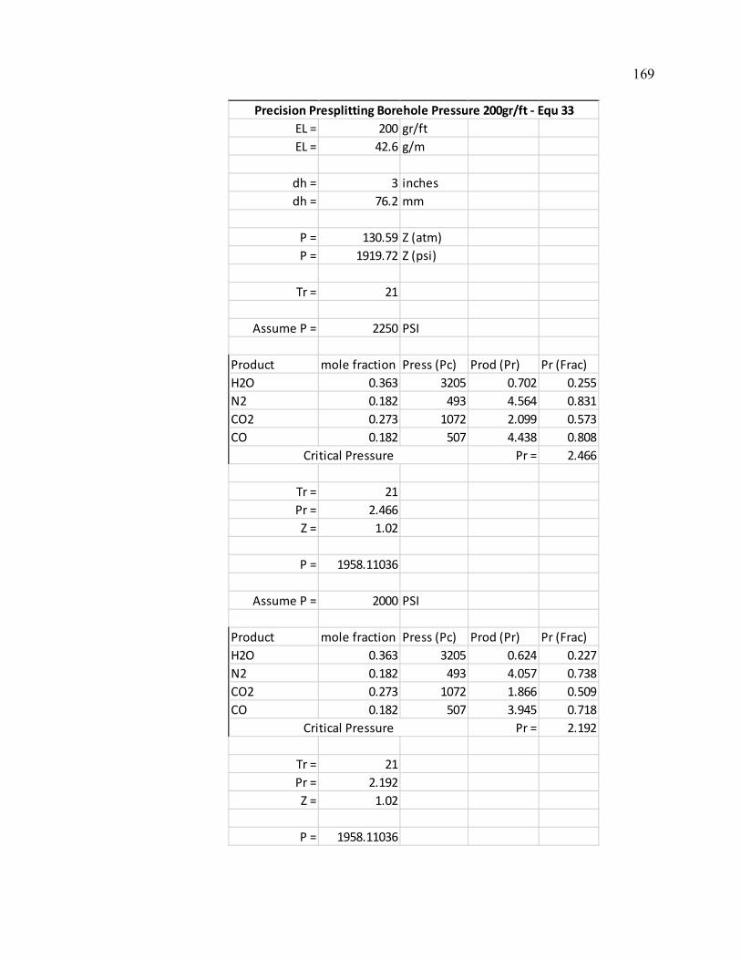
169
EL = 200 gr/ftEL = 42.6 g/m
dh = 3 inchesdh = 76.2 mm
P = 130.59 Z (atm)P = 1919.72 Z (psi)
Tr = 21
Assume P = 2250 PSI
Product mole fraction Press (Pc) Prod (Pr) Pr (Frac)H2O 0.363 3205 0.702 0.255N2 0.182 493 4.564 0.831CO2 0.273 1072 2.099 0.573CO 0.182 507 4.438 0.808
Pr = 2.466
Tr = 21Pr = 2.466Z = 1.02
P = 1958.11036
Assume P = 2000 PSI
Product mole fraction Press (Pc) Prod (Pr) Pr (Frac)H2O 0.363 3205 0.624 0.227N2 0.182 493 4.057 0.738CO2 0.273 1072 1.866 0.509CO 0.182 507 3.945 0.718
Pr = 2.192
Tr = 21Pr = 2.192Z = 1.02
P = 1958.11036
Critical Pressure
Critical Pressure
Precision Presplitting Borehole Pressure 200gr/ft - Equ 33

170
EL = 300 gr/ftEL = 63.9 g/m
dh = 3 inchesdh = 76.2 mm
P = 195.89 Z (atm)P = 2879.57 Z (psi)
Tr = 21
Assume P = 3000 PSI
Product mole fraction Press (Pc) Prod (Pr) Pr (Frac)H2O 0.363 3205 0.936 0.340N2 0.182 493 6.085 1.108CO2 0.273 1072 2.799 0.764CO 0.182 507 5.917 1.077
Pr = 3.288
Tr = 21Pr = 3.288Z = 1.03
P = 2965.961281
Assume P = 3000 PSI
Product mole fraction Press (Pc) Prod (Pr) Pr (Frac)H2O 0.363 3205 0.936 0.340N2 0.182 493 6.085 1.108CO2 0.273 1072 2.799 0.764CO 0.182 507 5.917 1.077
Pr = 3.288
Tr = 21Pr = 3.288Z = 1.03
P = 2965.961281
Precision Presplitting Borehole Pressure 300gr/ft - Equ 33
Critical Pressure
Critical Pressure

171
EL = 500 gr/ftEL = 106.5 g/m
dh = 3 inchesdh = 76.2 mm
P = 326.48 Z (atm)P = 4799.29 Z (psi)
Tr = 21
Assume P = 5000 PSI
Product mole fraction Press (Pc) Prod (Pr) Pr (Frac)H2O 0.363 3205 1.560 0.566N2 0.182 493 10.142 1.846CO2 0.273 1072 4.664 1.273CO 0.182 507 9.862 1.795
Pr = 5.480
Tr = 21Pr = 5.480Z = 1.04
P = 4991.261703
Assume P = 5000 PSI
Product mole fraction Press (Pc) Prod (Pr) Pr (Frac)H2O 0.363 3205 1.560 0.566N2 0.182 493 10.142 1.846CO2 0.273 1072 4.664 1.273CO 0.182 507 9.862 1.795
Pr = 5.480
Tr = 21Pr = 5.480Z = 1.04
P = 4991.261703
Critical Pressure
Critical Pressure
Precision Presplitting Borehole Pressure 500gr/ft - Equ 33

172
EL = 700 gr/ftEL = 149.1 g/m
dh = 3 inchesdh = 76.2 mm
P = 457.08 Z (atm)P = 6719.01 Z (psi)
Tr = 21
Assume P = 7000 PSI
Product mole fraction Press (Pc) Prod (Pr) Pr (Frac)H2O 0.363 3205 2.184 0.793N2 0.182 493 14.199 2.584CO2 0.273 1072 6.530 1.783CO 0.182 507 13.807 2.513
Pr = 7.672
Tr = 21Pr = 7.672Z = 1.05
P = 7054.956445
Assume P = 7000 PSI
Product mole fraction Press (Pc) Prod (Pr) Pr (Frac)H2O 0.363 3205 2.184 0.793N2 0.182 493 14.199 2.584CO2 0.273 1072 6.530 1.783CO 0.182 507 13.807 2.513
Pr = 7.672
Tr = 21Pr = 7.672Z = 1.05
P = 7054.956445
Precision Presplitting Borehole Pressure 700gr/ft - Equ 33
Critical Pressure
Critical Pressure

173
EL = 100 gr/ftEL = 21.3 g/m
dh = 2 inchesdh = 50.8 mm
P = 146.92 Z (atm)P = 2159.68 Z (psi)
Tr = 21
Assume P = 2250 PSI
Product mole fraction Press (Pc) Prod (Pr) Pr (Frac)H2O 0.363 3205 0.702 0.255N2 0.182 493 4.564 0.831CO2 0.273 1072 2.099 0.573CO 0.182 507 4.438 0.808
Pr = 2.466
Tr = 21Pr = 2.466Z = 1.02
P = 2202.874155
Assume P = 2200 PSI
Product mole fraction Press (Pc) Prod (Pr) Pr (Frac)H2O 0.363 3205 0.686 0.249N2 0.182 493 4.462 0.812CO2 0.273 1072 2.052 0.560CO 0.182 507 4.339 0.790
Pr = 2.411
Tr = 21Pr = 2.411Z = 1.02
P = 2202.874155
Precision Presplitting Borehole Pressure 100gr/ft - Equ 33
Critical Pressure
Critical Pressure

174
EL = 200 gr/ftEL = 42.6 g/m
dh = 2 inchesdh = 50.8 mm
P = 293.83 Z (atm)P = 4319.36 Z (psi)
Tr = 21
Assume P = 4500 PSI
Product mole fraction Press (Pc) Prod (Pr) Pr (Frac)H2O 0.363 3205 1.404 0.510N2 0.182 493 9.128 1.661CO2 0.273 1072 4.198 1.146CO 0.182 507 8.876 1.615
Pr = 4.932
Tr = 21Pr = 4.932Z = 1.04
P = 4492.135532
Assume P = 4500 PSI
Product mole fraction Press (Pc) Prod (Pr) Pr (Frac)H2O 0.363 3205 1.404 0.510N2 0.182 493 9.128 1.661CO2 0.273 1072 4.198 1.146CO 0.182 507 8.876 1.615
Pr = 4.932
Tr = 21Pr = 4.932Z = 1.04
P = 4492.135532
Precision Presplitting Borehole Pressure 200gr/ft - Equ 33
Critical Pressure
Critical Pressure

175
EL = 300 gr/ftEL = 63.9 g/m
dh = 2 inchesdh = 50.8 mm
P = 440.75 Z (atm)P = 6479.04 Z (psi)
Tr = 21
Assume P = 6500 PSI
Product mole fraction Press (Pc) Prod (Pr) Pr (Frac)H2O 0.363 3205 2.028 0.736N2 0.182 493 13.185 2.400CO2 0.273 1072 6.063 1.655CO 0.182 507 12.821 2.333
Pr = 7.124
Tr = 21Pr = 7.124Z = 1.05
P = 6802.993715
Assume P = 6800 PSI
Product mole fraction Press (Pc) Prod (Pr) Pr (Frac)H2O 0.363 3205 2.122 0.770N2 0.182 493 13.793 2.510CO2 0.273 1072 6.343 1.732CO 0.182 507 13.412 2.441
Pr = 7.453
Tr = 21Pr = 7.453Z = 1.05
P = 6802.993715
Precision Presplitting Borehole Pressure 300gr/ft - Equ 33
Critical Pressure
Critical Pressure

176
EL = 500 gr/ftEL = 106.5 g/m
dh = 2 inchesdh = 50.8 mm
P = 734.59 Z (atm)P = 10798.40 Z (psi)
Tr = 21
Assume P = 11000 PSI
Product mole fraction Press (Pc) Prod (Pr) Pr (Frac)H2O 0.363 3205 3.432 1.246N2 0.182 493 22.312 4.061CO2 0.273 1072 10.261 2.801CO 0.182 507 21.696 3.949
Pr = 12.057
Tr = 21Pr = 12.057Z = 1.06
P = 11446.30689
Assume P = 11500 PSI
Product mole fraction Press (Pc) Prod (Pr) Pr (Frac)H2O 0.363 3205 3.588 1.302N2 0.182 493 23.327 4.245CO2 0.273 1072 10.728 2.929CO 0.182 507 22.682 4.128
Pr = 12.605
Tr = 21Pr = 12.605Z = 1.07
P = 11554.29091
Precision Presplitting Borehole Pressure 500gr/ft - Equ 33
Critical Pressure
Critical Pressure

177
EL = 700 gr/ftEL = 149.1 g/m
dh = 2 inchesdh = 50.8 mm
P = 1028.42 Z (atm)P = 15117.76 Z (psi)
Tr = 21
Assume P = 16750 PSI
Product mole fraction Press (Pc) Prod (Pr) Pr (Frac)H2O 0.363 3205 5.226 1.897N2 0.182 493 33.976 6.184CO2 0.273 1072 15.625 4.266CO 0.182 507 33.037 6.013
Pr = 18.359
Tr = 21Pr = 18.359Z = 1.1
P = 16629.54019
Assume P = 16630 PSI
Product mole fraction Press (Pc) Prod (Pr) Pr (Frac)H2O 0.363 3205 5.189 1.884N2 0.182 493 33.732 6.139CO2 0.273 1072 15.513 4.235CO 0.182 507 32.801 5.970
Pr = 18.228
Tr = 21Pr = 18.228Z = 1.1
P = 16629.54019
Precision Presplitting Borehole Pressure 700gr/ft - Equ 33
Critical Pressure
Critical Pressure
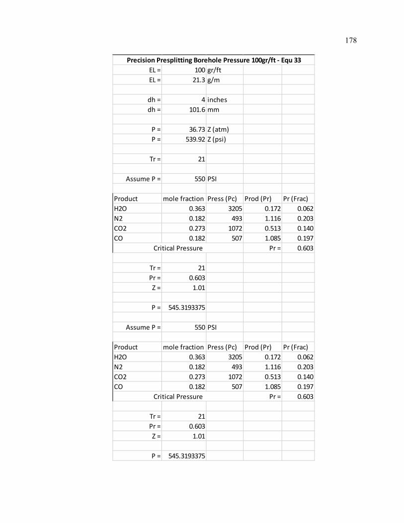
178
EL = 100 gr/ftEL = 21.3 g/m
dh = 4 inchesdh = 101.6 mm
P = 36.73 Z (atm)P = 539.92 Z (psi)
Tr = 21
Assume P = 550 PSI
Product mole fraction Press (Pc) Prod (Pr) Pr (Frac)H2O 0.363 3205 0.172 0.062N2 0.182 493 1.116 0.203CO2 0.273 1072 0.513 0.140CO 0.182 507 1.085 0.197
Pr = 0.603
Tr = 21Pr = 0.603Z = 1.01
P = 545.3193375
Assume P = 550 PSI
Product mole fraction Press (Pc) Prod (Pr) Pr (Frac)H2O 0.363 3205 0.172 0.062N2 0.182 493 1.116 0.203CO2 0.273 1072 0.513 0.140CO 0.182 507 1.085 0.197
Pr = 0.603
Tr = 21Pr = 0.603Z = 1.01
P = 545.3193375
Precision Presplitting Borehole Pressure 100gr/ft - Equ 33
Critical Pressure
Critical Pressure
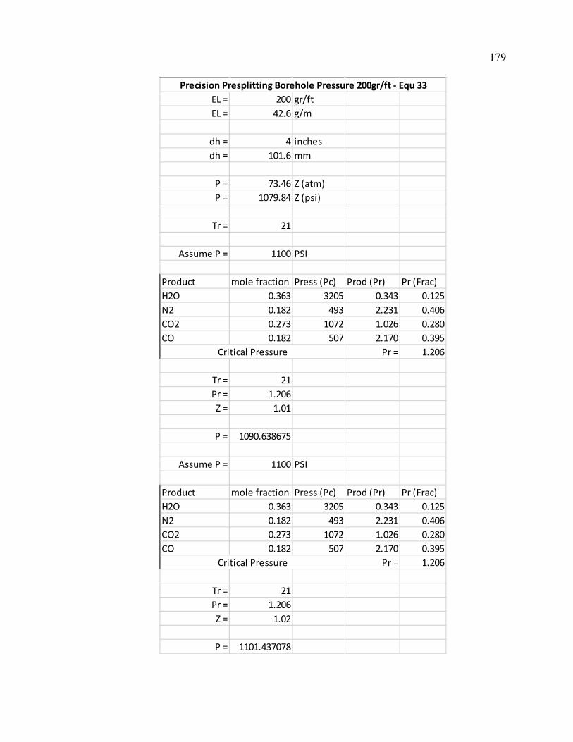
179
EL = 200 gr/ftEL = 42.6 g/m
dh = 4 inchesdh = 101.6 mm
P = 73.46 Z (atm)P = 1079.84 Z (psi)
Tr = 21
Assume P = 1100 PSI
Product mole fraction Press (Pc) Prod (Pr) Pr (Frac)H2O 0.363 3205 0.343 0.125N2 0.182 493 2.231 0.406CO2 0.273 1072 1.026 0.280CO 0.182 507 2.170 0.395
Pr = 1.206
Tr = 21Pr = 1.206Z = 1.01
P = 1090.638675
Assume P = 1100 PSI
Product mole fraction Press (Pc) Prod (Pr) Pr (Frac)H2O 0.363 3205 0.343 0.125N2 0.182 493 2.231 0.406CO2 0.273 1072 1.026 0.280CO 0.182 507 2.170 0.395
Pr = 1.206
Tr = 21Pr = 1.206Z = 1.02
P = 1101.437078
Precision Presplitting Borehole Pressure 200gr/ft - Equ 33
Critical Pressure
Critical Pressure

180
EL = 300 gr/ftEL = 63.9 g/m
dh = 4 inchesdh = 101.6 mm
P = 110.19 Z (atm)P = 1619.76 Z (psi)
Tr = 21
Assume P = 1700 PSI
Product mole fraction Press (Pc) Prod (Pr) Pr (Frac)H2O 0.363 3205 0.530 0.193N2 0.182 493 3.448 0.628CO2 0.273 1072 1.586 0.433CO 0.182 507 3.353 0.610
Pr = 1.863
Tr = 21Pr = 1.863Z = 1.01
P = 1635.958012
Assume P = 1650 PSI
Product mole fraction Press (Pc) Prod (Pr) Pr (Frac)H2O 0.363 3205 0.515 0.187N2 0.182 493 3.347 0.609CO2 0.273 1072 1.539 0.420CO 0.182 507 3.254 0.592
Pr = 1.809
Tr = 21Pr = 1.809Z = 1.01
P = 1635.958012
Critical Pressure
Critical Pressure
Precision Presplitting Borehole Pressure 300gr/ft - Equ 33

181
EL = 500 gr/ftEL = 106.5 g/m
dh = 4 inchesdh = 101.6 mm
P = 183.65 Z (atm)P = 2699.60 Z (psi)
Tr = 21
Assume P = 2750 PSI
Product mole fraction Press (Pc) Prod (Pr) Pr (Frac)H2O 0.363 3205 0.858 0.311N2 0.182 493 5.578 1.015CO2 0.273 1072 2.565 0.700CO 0.182 507 5.424 0.987
Pr = 3.014
Tr = 21Pr = 3.014Z = 1.02
P = 2753.592694
Assume P = 2750 PSI
Product mole fraction Press (Pc) Prod (Pr) Pr (Frac)H2O 0.363 3205 0.858 0.311N2 0.182 493 5.578 1.015CO2 0.273 1072 2.565 0.700CO 0.182 507 5.424 0.987
Pr = 3.014
Tr = 21Pr = 3.014Z = 1.02
P = 2753.592694
Precision Presplitting Borehole Pressure 500gr/ft - Equ 33
Critical Pressure
Critical Pressure
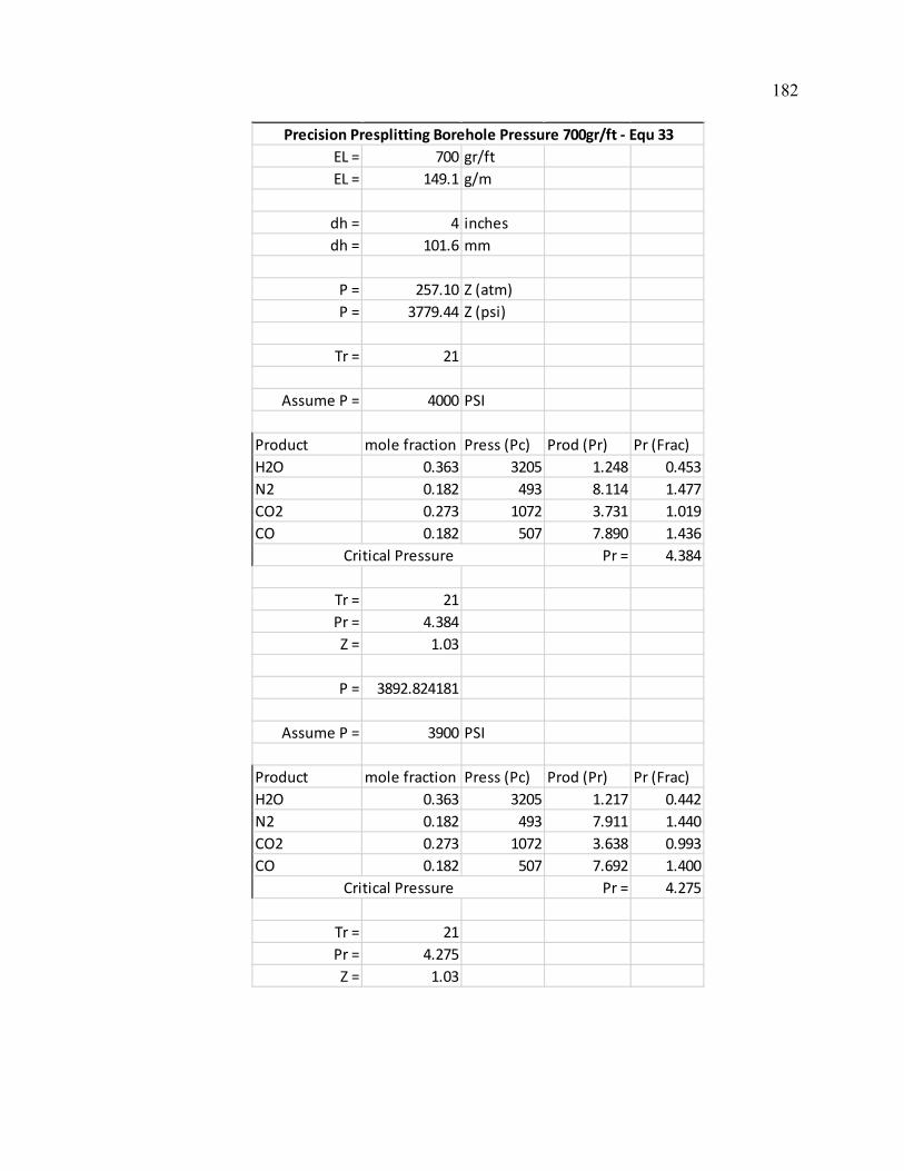
182
EL = 700 gr/ftEL = 149.1 g/m
dh = 4 inchesdh = 101.6 mm
P = 257.10 Z (atm)P = 3779.44 Z (psi)
Tr = 21
Assume P = 4000 PSI
Product mole fraction Press (Pc) Prod (Pr) Pr (Frac)H2O 0.363 3205 1.248 0.453N2 0.182 493 8.114 1.477CO2 0.273 1072 3.731 1.019CO 0.182 507 7.890 1.436
Pr = 4.384
Tr = 21Pr = 4.384Z = 1.03
P = 3892.824181
Assume P = 3900 PSI
Product mole fraction Press (Pc) Prod (Pr) Pr (Frac)H2O 0.363 3205 1.217 0.442N2 0.182 493 7.911 1.440CO2 0.273 1072 3.638 0.993CO 0.182 507 7.692 1.400
Pr = 4.275
Tr = 21Pr = 4.275Z = 1.03
Critical Pressure
Critical Pressure
Precision Presplitting Borehole Pressure 700gr/ft - Equ 33

183
EL = 100 gr/ftEL = 21.3 g/m
dh = 1.5 inchesdh = 38.1 mm
P = 261.19 Z (atm)P = 3839.43 Z (psi)
Tr = 21
Assume P = 4000 PSI
Product mole fraction Press (Pc) Prod (Pr) Pr (Frac)H2O 0.363 3205 1.248 0.453N2 0.182 493 8.114 1.477CO2 0.273 1072 3.731 1.019CO 0.182 507 7.890 1.436
Pr = 4.384
Tr = 21Pr = 4.384Z = 1.03
P = 3954.615041
Assume P = 4000 PSI
Product mole fraction Press (Pc) Prod (Pr) Pr (Frac)H2O 0.363 3205 1.248 0.453N2 0.182 493 8.114 1.477CO2 0.273 1072 3.731 1.019CO 0.182 507 7.890 1.436
Pr = 4.384
Tr = 21Pr = 4.384Z = 1.03
P = 3954.615041
Precision Presplitting Borehole Pressure 100gr/ft - Equ 33
Critical Pressure
Critical Pressure

184
EL = 200 gr/ftEL = 42.6 g/m
dh = 1.5 inchesdh = 38.1 mm
P = 522.37 Z (atm)P = 7678.86 Z (psi)
Tr = 21
Assume P = 8000 PSI
Product mole fraction Press (Pc) Prod (Pr) Pr (Frac)H2O 0.363 3205 2.496 0.906N2 0.182 493 16.227 2.953CO2 0.273 1072 7.463 2.037CO 0.182 507 15.779 2.872
Pr = 8.769
Tr = 21Pr = 8.769Z = 1.05
P = 8062.807366
Assume P = 8050 PSI
Product mole fraction Press (Pc) Prod (Pr) Pr (Frac)H2O 0.363 3205 2.512 0.912N2 0.182 493 16.329 2.972CO2 0.273 1072 7.509 2.050CO 0.182 507 15.878 2.890
Pr = 8.823
Tr = 21Pr = 8.823Z = 1.05
P = 8062.807366
Precision Presplitting Borehole Pressure 200gr/ft - Equ 33
Critical Pressure
Critical Pressure

185
EL = 300 gr/ftEL = 63.9 g/m
dh = 1.5 inchesdh = 38.1 mm
P = 783.56 Z (atm)P = 11518.30 Z (psi)
Tr = 21
Assume P = 12500 PSI
Product mole fraction Press (Pc) Prod (Pr) Pr (Frac)H2O 0.363 3205 3.900 1.416N2 0.182 493 25.355 4.615CO2 0.273 1072 11.660 3.183CO 0.182 507 24.655 4.487
Pr = 13.701
Tr = 21Pr = 13.701Z = 1.07
P = 12324.57697
Assume P = 12350 PSI
Product mole fraction Press (Pc) Prod (Pr) Pr (Frac)H2O 0.363 3205 3.853 1.399N2 0.182 493 25.051 4.559CO2 0.273 1072 11.521 3.145CO 0.182 507 24.359 4.433
Pr = 13.536
Tr = 21Pr = 13.536Z = 1.07
P = 12324.57697
Critical Pressure
Precision Presplitting Borehole Pressure 300gr/ft - Equ 33
Critical Pressure
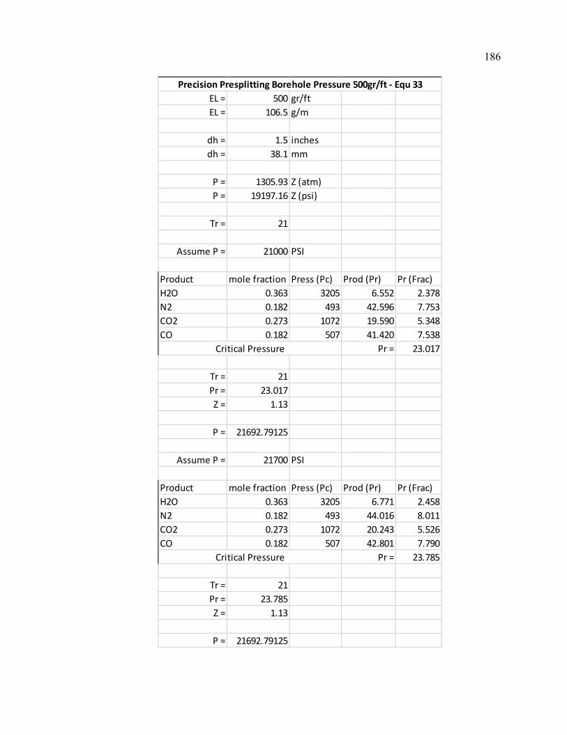
186
EL = 500 gr/ftEL = 106.5 g/m
dh = 1.5 inchesdh = 38.1 mm
P = 1305.93 Z (atm)P = 19197.16 Z (psi)
Tr = 21
Assume P = 21000 PSI
Product mole fraction Press (Pc) Prod (Pr) Pr (Frac)H2O 0.363 3205 6.552 2.378N2 0.182 493 42.596 7.753CO2 0.273 1072 19.590 5.348CO 0.182 507 41.420 7.538
Pr = 23.017
Tr = 21Pr = 23.017Z = 1.13
P = 21692.79125
Assume P = 21700 PSI
Product mole fraction Press (Pc) Prod (Pr) Pr (Frac)H2O 0.363 3205 6.771 2.458N2 0.182 493 44.016 8.011CO2 0.273 1072 20.243 5.526CO 0.182 507 42.801 7.790
Pr = 23.785
Tr = 21Pr = 23.785Z = 1.13
P = 21692.79125
Precision Presplitting Borehole Pressure 500gr/ft - Equ 33
Critical Pressure
Critical Pressure
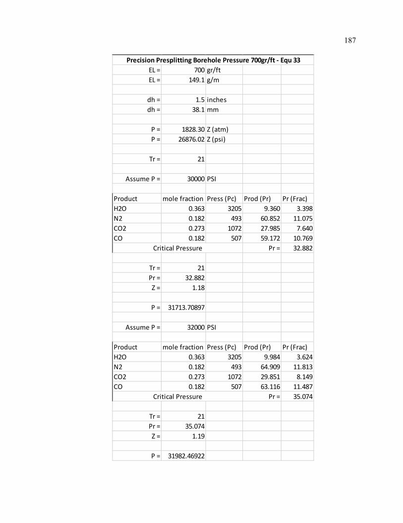
187
EL = 700 gr/ftEL = 149.1 g/m
dh = 1.5 inchesdh = 38.1 mm
P = 1828.30 Z (atm)P = 26876.02 Z (psi)
Tr = 21
Assume P = 30000 PSI
Product mole fraction Press (Pc) Prod (Pr) Pr (Frac)H2O 0.363 3205 9.360 3.398N2 0.182 493 60.852 11.075CO2 0.273 1072 27.985 7.640CO 0.182 507 59.172 10.769
Pr = 32.882
Tr = 21Pr = 32.882Z = 1.18
P = 31713.70897
Assume P = 32000 PSI
Product mole fraction Press (Pc) Prod (Pr) Pr (Frac)H2O 0.363 3205 9.984 3.624N2 0.182 493 64.909 11.813CO2 0.273 1072 29.851 8.149CO 0.182 507 63.116 11.487
Pr = 35.074
Tr = 21Pr = 35.074Z = 1.19
P = 31982.46922
Critical Pressure
Precision Presplitting Borehole Pressure 700gr/ft - Equ 33
Critical Pressure

188
APPENDIX C.
VALIDATION OF ISOTHERMAL ASSUMPTION
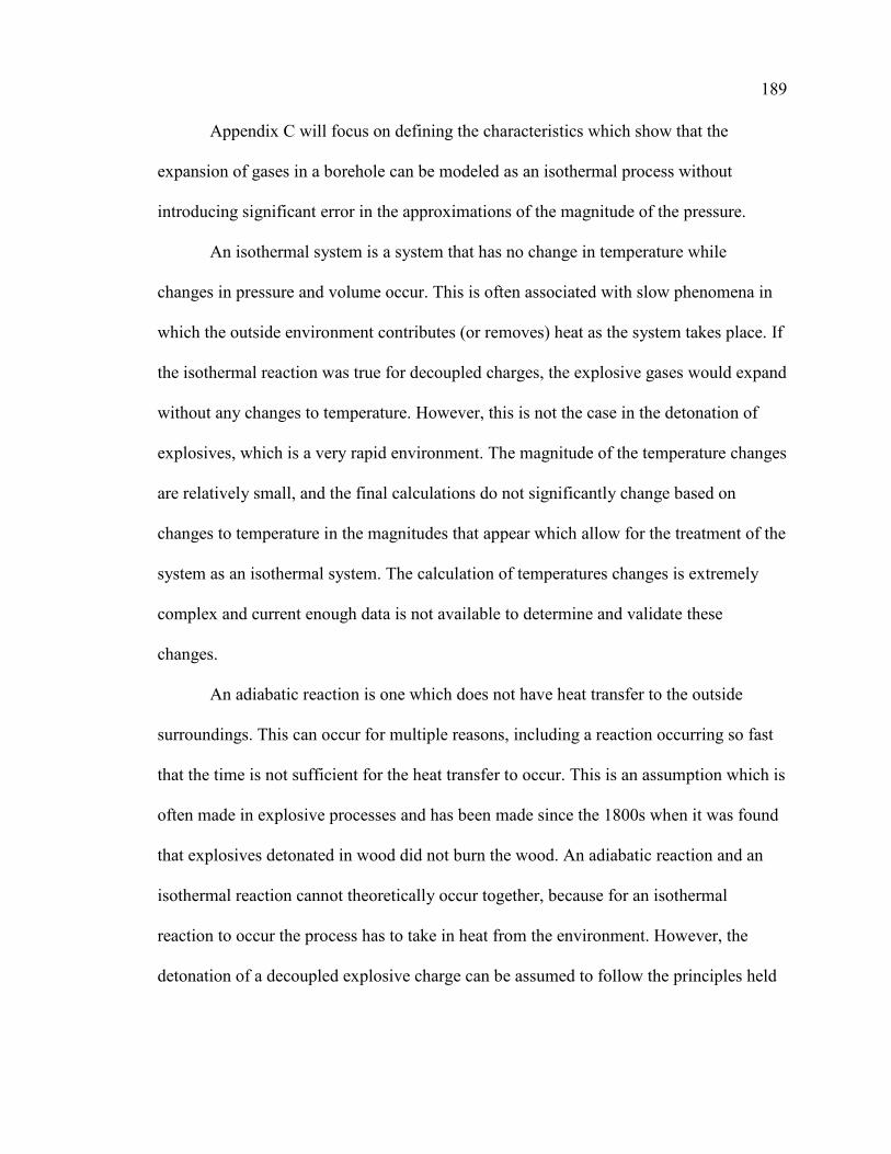
189
Appendix C will focus on defining the characteristics which show that the
expansion of gases in a borehole can be modeled as an isothermal process without
introducing significant error in the approximations of the magnitude of the pressure.
An isothermal system is a system that has no change in temperature while
changes in pressure and volume occur. This is often associated with slow phenomena in
which the outside environment contributes (or removes) heat as the system takes place. If
the isothermal reaction was true for decoupled charges, the explosive gases would expand
without any changes to temperature. However, this is not the case in the detonation of
explosives, which is a very rapid environment. The magnitude of the temperature changes
are relatively small, and the final calculations do not significantly change based on
changes to temperature in the magnitudes that appear which allow for the treatment of the
system as an isothermal system. The calculation of temperatures changes is extremely
complex and current enough data is not available to determine and validate these
changes.
An adiabatic reaction is one which does not have heat transfer to the outside
surroundings. This can occur for multiple reasons, including a reaction occurring so fast
that the time is not sufficient for the heat transfer to occur. This is an assumption which is
often made in explosive processes and has been made since the 1800s when it was found
that explosives detonated in wood did not burn the wood. An adiabatic reaction and an
isothermal reaction cannot theoretically occur together, because for an isothermal
reaction to occur the process has to take in heat from the environment. However, the
detonation of a decoupled explosive charge can be assumed to follow the principles held
190
in both; this allows for the disregard of heat transfer from the high temperature gas to the
rock mass and the use of Boyle’s law to determine pressure at changes in volume.
It is important to address the actual gas dynamics which occur in the borehole
from a decoupled charge. When the explosive detonates the solid chemicals are converted
to a plasma which have a diameter smaller than that of the original explosive charge
(Cook M. A., 1974). At this point, the gases are considered to be at the temperature of the
explosion, Te, which is calculated in section 4.1 of this dissertation. As the gases expand,
the temperature decreases. When the gases impact the borehole wall, the temperature is
raised due to a stagnation effect if the gases are traveling at a supersonic speed. It is
currently unknown at what distance away from the charge this ceases to exist. If the gas
is not traveling at a supersonic speed, then the heat sources are (Baird, 2019):
• The combined heat from the detonation
• The compressive heating causes by the passage of the air shock created by
the detonation front
The air shock or the stagnation effect would both cause increases to the
temperature which would likely be equivalent to losses from expansion.
The changes in temperature can also be modelled from a simplified approach
which is used on rarefield gases which are released into a vacuum (Molmud, 1960;
Zel'dovich & Raizer, 2002). This is completed using Equation C.1.
∆𝑇𝑇 = 𝑓𝑓−3(𝛾𝛾−1) (C.1)
where ΔT is the change in temperature in ° K, t is time in seconds, γ is the specific heat
ratio which for these gases has been determined to be 1.2. At maximum γ can be 1.66,
which takes place at complete freezing of internal degrees of freedom.
191
The importance of the temperature change occurs when the maximum pressure is
calculated. This corresponds to a time of 0.1ms to 0.3ms (Otuonye, 1981). Using
Equation A3-1, this results in a change in temperature of 50° K to 250° K; with a typical
change in temperature of between 100° K to 150° K. This is considered minimal when
considering a temperature of explosion for PETN of 4900° K.
A sensitivity analysis can be completed to view how a change in 100° K would
affect the borehole pressure. This can be completed using Equation C.2
𝑃𝑃1𝑉𝑉1𝑇𝑇1
= 𝑃𝑃2𝑉𝑉2𝑇𝑇2
(C.2)
where P1 is the original pressure in psi, V1 is the original volume in L, T1 is the original
temperature in °K, P2 is the final pressure in psi, V2 is the final volume in L, and T2 is the
final temperature in ° K. Assuming that P1 is 10,000 psi, V1 is 0.067 L, T1 is 4900° K, V2
is 0.257L, and T2 is 4800°K, the final pressure can be computed.
10000 ∗ 0.0674900
= 𝑃𝑃2 ∗ 0.257
4800
P2 is then equal to 2554 psi.
The process can be completed with the assumption of isothermal conditions and using
Boyle’s Law, which is presented again as Equation C.3
𝑃𝑃1𝑉𝑉1 = 𝑃𝑃2𝑉𝑉2 (C.3)
Using the same pressure and volumes as before, the final pressure can be
calculated, as shown below.
10,000 ∗ 0.067 = 𝑃𝑃2 ∗ 0.257
P2 is then equal to 2,607 psi.
192
The difference in pressure between taking into account the temperature difference
associated with the gas expansion result in an error in the calculation of the borehole
pressure of 2%. This can be considered minimal and insignificant compared to other
potential sources of error.
Furthermore, other authors have treated the detonation and expansion of the gases
as an isothermal process and found good agreement with the measured data for borehole
pressures (Otuonye, Skidmore, & Konya, 1983). This confirms that the assumption of the
isothermal process results in minimal error. This has also been validated in this
dissertation by the use of the explosion temperature in the Thermodynamic Model for
borehole pressure calculations. The temperature used in this equation is the explosion
temperature and this shows excellent fit of data with the measured results. If treatment of
the process as isothermal introduced significant error, then this would cause incorrect
prediction of the borehole pressure. Instead, the temperature of the gases after expansion
volume expansion would be required. This goes to prove that while the process is not
perfectly isothermal, it can be modeled as isothermal without introducing major error.
193
APPENDIX D.
CIRCUMFERENTIAL STRESSES AROUND A BOREHOLE
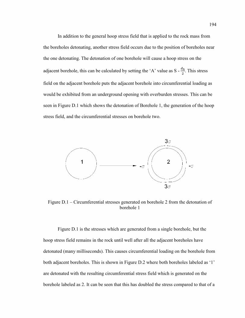
194
In addition to the general hoop stress field that is applied to the rock mass from
the boreholes detonating, another stress field occurs due to the position of boreholes near
the one detonating. The detonation of one borehole will cause a hoop stress on the
adjacent borehole, this can be calculated by setting the ‘A’ value as S - 𝑑𝑑ℎ2
. This stress
field on the adjacent borehole puts the adjacent borehole into circumferential loading as
would be exhibited from an underground opening with overburden stresses. This can be
seen in Figure D.1 which shows the detonation of Borehole 1, the generation of the hoop
stress field, and the circumferential stresses on borehole two.
Figure D.1 – Circumferential stresses generated on borehole 2 from the detonation of borehole 1
Figure D.1 is the stresses which are generated from a single borehole, but the
hoop stress field remains in the rock until well after all the adjacent boreholes have
detonated (many milliseconds). This causes circumferential loading on the borehole from
both adjacent boreholes. This is shown in Figure D.2 where both boreholes labeled as ‘1’
are detonated with the resulting circumferential stress field which is generated on the
borehole labeled as 2. It can be seen that this has doubled the stress compared to that of a
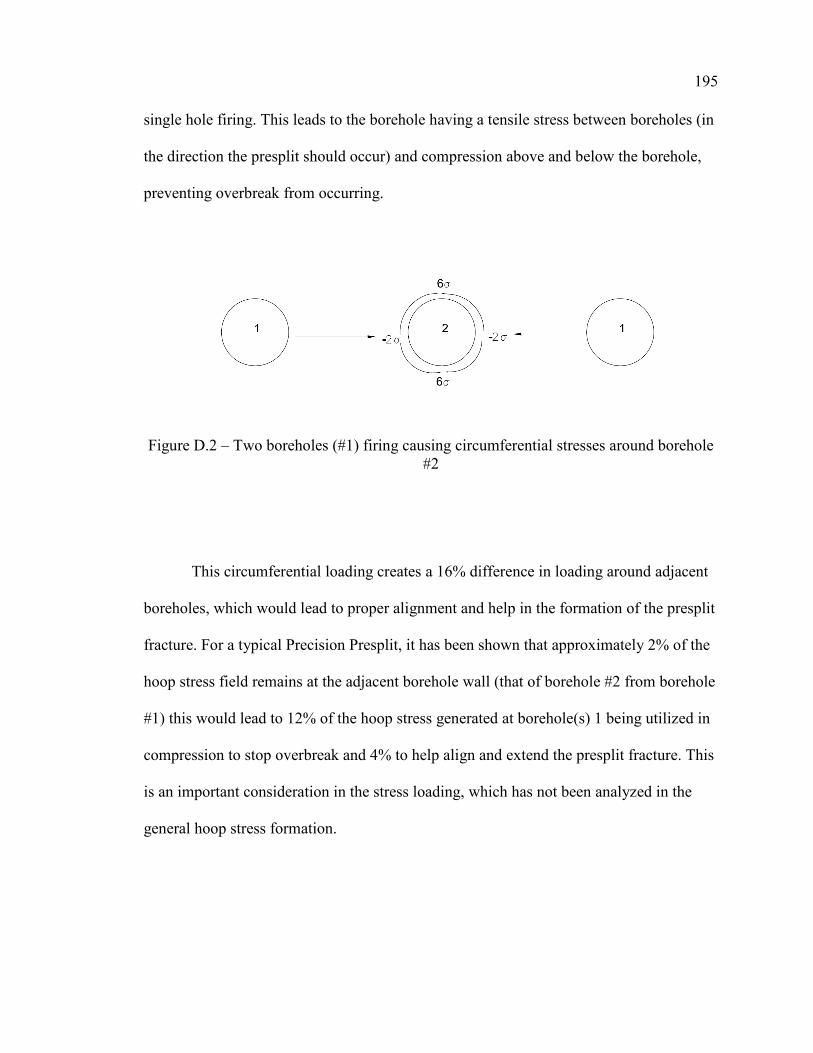
195
single hole firing. This leads to the borehole having a tensile stress between boreholes (in
the direction the presplit should occur) and compression above and below the borehole,
preventing overbreak from occurring.
Figure D.2 – Two boreholes (#1) firing causing circumferential stresses around borehole #2
This circumferential loading creates a 16% difference in loading around adjacent
boreholes, which would lead to proper alignment and help in the formation of the presplit
fracture. For a typical Precision Presplit, it has been shown that approximately 2% of the
hoop stress field remains at the adjacent borehole wall (that of borehole #2 from borehole
#1) this would lead to 12% of the hoop stress generated at borehole(s) 1 being utilized in
compression to stop overbreak and 4% to help align and extend the presplit fracture. This
is an important consideration in the stress loading, which has not been analyzed in the
general hoop stress formation.

196
BIBLIOGRAPHY
Akhavan, J. (2011). The Chemistry of Explosives. Cambridge: RSC Publishing.
Andre, G. G. (1878). Rock Blasting. A Practical Treatise on the Means Employed in Blasting Rocks for Industrial Purposes. London: E. & F.N. Spon.
Ash, R. (1963a, August). Mechanics of Rock Breakage - Part 1. Pit and Quarry, 98-112.
Ash, R. (1963b, September). Mechanics of Rock Breakage - Part 2. Pit and Quarry, 118-123.
Ash, R. (1973). The Influence of Geological Discontinuities on Rock Blasting - Doctoral Thesis. University of Minnesota.
Ash, R. (1974). Considerations for Proper Blasting Design. Second Annual Blasting Conference of the Kentucky Dept of Mines and Minerals, 45-59.
Bacon, R. (1733). Fratris Rogeri Bacon, ordinis Minorum, opus majus ad Clementem IV, pontificem Romanum. (R. Burke, Trans.) London.
Baird, J. (2019, October). Personal Communication.
Bauer, A., Harris, G., Lang, L., Preziosi, P., & Selleck, D. (1965, September). How IOC Puts Crater Research to Work. Engineering and Mining Journal, 166(9), 117-121.
Becher, J. (1667). Physica Subterranea.
Becker, R. (1922a). Physikalisches uber feste und gasformige Sprengstoffe. Z. Techn. Phys., 4, 152.
Becker, R. (1922b). Stosswlle and Detonation. Zs. Phys., 8, 321.
Becker, R. (1929). Impact, Waves and Detonation.
Ben-Dor, G., & Takayama, K. (1992). The Phenomena of Shock Wave Reflection - a Review of Unsolved problems and Future Research Needs. Shock Waves.
Berthelot, P. (1881). Sur la vitesse de propagation des phenomenes explosifs dans les gaz. C. R. Acad. Sci, 18-22.
Berthelot, P. (1892). Explosives and Their Power. London: John Murray.
Berthollet, C. (1786). Observations sur quelques combinaisons de l'acide marin dephlogistique ou de l'acide muriatique oxygene. Acad. Roy Sci., 385-396.
197
Biot, J. (1802). Theorie mathematique de la propagation du son. J. Phys. Theor. Appl., 173-182.
Boufadi, F., Bidai, K., Ameri, M., Bentouaf, A., Bensaid, D., Azzaz, Y., & Ameri, I. (2016). First Principles Study of Mechanical Stability and Thermodyanmics Properties of K2S under Pressure and Temperature Effect. Act Physica Series, 315-322.
Brinkley, S. R., & Kirkwood, J. G. (1947a). Theory of the Propagation of Shock Waves. Physical Review, 71(9), 606-611.
Brinkley, S. R., & Kirkwood, J. G. (1947b). Theory of the Propagation of Shock Waves from Infinite Cylinders of Explosives. Physical Review, 72(11), 1109-1113.
Brinkley, S., & Wilson Jr., E. (1942). Revised Method of Predicting the Detonation Velocities of Solid Explosives.
Brode, H. (1947). A Calculation of the Blast Wave from a Sphereical Charge of TNT: Rand Corporation Research Memorandum (RM-1965). Santa Monica.
Brown, E. M. (1673). Brief Account of some Travels in Hungaria as also some observations on Gold, Silver, Copper, Quick-filver Mines, Baths, and Mineral Waters. London: T.R.
Brown, M., & Rugunanan, R. (1989). A Temperature-Profile Study of the Combustion of Black Powder and its Constituent Binary Mixtures. Propellants, Explosives, Pyrotechnics, 69-75.
Burgoyne, J. (1874). A Treatise on the Blasting and Quarrying of stone for Building and Other Purposes. London: Crosby Lockwood and Co.
Cevizci, H., & Ozkahraman, H. (2012). The effect of Blast Hole Stemming Length to Rockpile Fragmentation at Limestone Quarries. International Journal of Rock Mecahnics and Mining Science.
Christoffel, E. (1877a). Fortpflanzung von Stoben durch elastische feste Korper. Ann. di Mat. Pura Appl, 193-243.
Christoffel, E. (1877b). Untersucheungen uber die mit dem Forbestehen linearer partieller Differentialgleichungen vertraglichen Unstetigkeiten. Ann. di Met. Pura Appl., 81-112.
Cole, R. (1948). Underwater Explosions. Princeton: Princeton University Press.
Cook, M. (1947). An Equation of State for Gases at Extremely High Pressure and Temperature for the Hydrodynamic Theory of Detonation. J. Chem. Phys., 518.
Cook, M. (1958). The Science of High Explosives. New York: Reinhold Publishing Corp.
198
Cook, M. A. (1974). The Science of Industrial Explosives. Salt Lake City: IRECO Chemicals.
Cooper, P. (1996). Explosive Engineering. New York, New York: VCH Publishers Inc.
Cosgrove, J. (1913). Rock Excavating and Blasting. Pittsburgh: J.J. Cosgrove.
Count of Rumford, B. (1797). Experiments to Determine the Force of Fired Gunpowder. Phil. Trans. Roy Soc, 222-294.
Cranz, C. (1926). Lehrbuch der Ballistik: II Innere Ballistik. Berlin: Springer.
Croll, O. (1609). Osvaldi Crollii Basilica chymica. Geneva.
Crosby, W., & Bauer, A. (1982). Wall Control Blasting in Open Pits. Mining Engineering, 34(2), 155-158.
Crussard, L. (1907). Ondes de choc et onde explosive. Bull. Soc. Industrie Minerale, 257-364.
Daehnke, A., Rossmanith, H., & Kouzniak, N. (1996, June). Dynamic Fracture Propagation due to Blast-Induced High Pressure Gas Loading. 2nd North American Rock Mechanics Symposium.
Daw, A., & Daw, Z. (1898). The Blasting of Rocks in Mines, Quarries, Tunnels, Etc. London: E. & F.N.
Day, P. (1982). Controlled Blasting to Minimize Overbrak with Big Boreholes Underground. Proceedings of the Eighth Conference on Explosives and Blasting Technique, 264-274.
De Lagrange, J. (1781). Memoire sur la theorie du mouvement des fluides. Acad. Roy. Sci. & Belles Lettres, 151-198.
Dodge, B. (1944). Chemical Engineering Thermodynamics. New York: McGraw-Hill.
Duhem, P. M. (1909). Sur la propagation des ondes de choc au sein des fluides. Z. Physik. Chem, 169-186.
DuPont. (1975). DuPont Blasters Handbook. DuPont.
Duvall, W. (1953). Strain-Wave Shapes in Rock Near Explosions. Geophysics, 18, 310-323.
Duvall, W., & Atchison, T. (1957). Rock Breakage by Explosives. U.S. Bureau of Mines.
Duvall, W., & Petkof, B. (1959). Spherical Propagation of Explosion Generated Strain Pulses in Rock. U.S. Bureau of Mines.
199
Einstein, A. (1906). Theorie der Strahlung und die Theorie der Spezifischen Warme. Annalen der Physik, 180-190.
Euler, L. (1759). Euler's two letters to Lagrange. (C. I. Truesdell, Trans.)
Fenning, R., & Whiffin, A. (1939). The Specific Heat of Gases at High Temperatures. Phil. Trans. Roy. Soc., 149-228.
Goodman, R. (2014). Introduction to Rock Mechanics - 2nd Edition. John Wiley & Sons Inc.
Grant, C. (1964, November). Simplified Explanation of Crater Method. Engineering and Mining Journal, 165(11), 84-89.
Guttmann, O. (1892). Blasting: A Handbook for the Use of Engineering and Others Engaged in Mining, Tunnelling, Quarrying, etc. London: Charles Griffin and Company.
Harari, Y. N. (2011). Sapiens: A Brief History of Humankind. Isreal.
Hino, K. (1959). Theory and Practice of Blasting. Japan: Nippon Kayaku Co.
Hire, D. L. (1702). Unknown Title.
Hoek, E., Marinos, P., & Marinos, V. (n.d.). Characterization and engineering properties of tectonically undisturbed but lithologically varied sedimentary rock masses. International Journal of Rock Mechanics and Mining Science.
Hugoniot, P. (1887). Memoire sur la propagation du mouvement dans les corps et plus specialement dans les gaz parfaits. Partie. J. Ecole Polytech, 3-97.
Hutton, C. (1778). The Force of Fired Gunpowder. Phil. Trans. Roy. Soc., 50-85.
International Society of Explosive Engineers. (2016). Blasters Handbook 18th Edition. International Society of Explosive Engineers.
Jaffe, B. (1930). Crucibles: The Story of Chemistry. New York: Simon and Schuster.
Jeremic, J. (1994). Rock Mechanics in Salt Mining. Netherlands: Rotterdam.
Johansson, C., & Persson, P. (1970). Detonics of High Explosives. New York: Academic Press.
Johnson, G., & Steele, W. (1981). The standard enthalpy of formation of potassium sulfide by flourine bomb calorimetry. The Journal of Chmical Thermodyanmics, 985-990.

200
Johnson, N. (1974). Explosives. In Macropaedia, Encyclopedia Britannica (Vol. 7, p. 85). Chicago: Benton & Hemingway.
Johnson, S. (1971). NCG Technical Report No. 21. Livermore, California: U.S. Army Engineer Nuclear Cratering Group.
Johnsson, G., & Hofmeister, W. (1961, February). The Influence of Stemming on the Efficiency of Blasting. (G. Clark, Ed.) Proceddings of the International Symposium on Mining Research, 91-102.
Jouget, E. (1906). Sur la propagation des reactions chimiques dans les gaz. J. Math Pures Appl., 347-425.
Jouget, E. (1917). Mechanics of Explosives. Paris: O. Dion & Fils.
Jouguet, E. (1904). Sur l'onde explosive. C.R. Acad. Sci, 121-124.
Kapoor, S. (1970). Berthollet, Claude-Louis. In C. Gillespie, Dictionary of Scientific Biography (pp. 73-82). New York: Scribner's Sons.
Kirk, R., & Othmer, D. (1947). Encyclopedia of Chemical Technology. New York: The Interscience Encyclopedia Inc.
Kistiakowsky, G., & Wilson Jr., E. (1941a). Report on the Prediction of Detonation Velocities of Solid Explosives.
Kistiakowsky, G., & Wilson Jr., E. (1941b). The Hydrodyanmic Theory of Detonation and Shock Waves.
Klapotke, T. (2012). Chemistry of High-Energy Materials. Berlin: Walter de Gruyter.
Kojovic, T. (2005). Investigation of Aggregate Stemming in Blasting on SAG Mill Performance. Minerals Engineering, 1398-1404.
Konya, A. J., & Konya, C. J. (2017a). Precision Presplitting. Proceedings of the Society for Mining, Metallurgy, and Exploration.
Konya, A., & Konya, C. (2017b). Precision Presplitting - Explosive Variations with Spacing. Proceedings of the 43rd International Conference on Explosive and Blasting Technique.
Konya, A., & Konya, C. J. (2016). Precision Presplitting Optimization. Proceedings of the Forty-Second Annual Conference on Explosives and Blasting Technique (pp. 65-74). Las Vegas: International Society of Explosive Engineers.
Konya, C. (1973). High Speed Photographic Analysis of the Mechanics of Presplit Blasting. Proceedings of Sprengtechnick International.
201
Konya, C. (1980). Pre-split Blasting: Theory and Practice. Preprint AIME, 80-97.
Konya, C. (1982). Seminar on Blasting to the Ohio Laborers Union. Mont Vernon, Ohio.
Konya, C. (2015). Rock Blasting and Overbreak Control. Montville: Academy of Blasting and Explosive Technology.
Konya, C., & Konya, A. (2015, November). Precision Presplitting Optimization. 8th Drilling-Blasting Symposium, (pp. 1-10). Istanbul, Turkey.
Konya, C., & Konya, A. (2018). Effect of Hole Stemming Practices on Energy Efficiency of Comminution. In K. Awuah-Offei, Energy Efficiency in the Minerals Industry (pp. 31-54). Springer.
Konya, C., Barret, D., & Smith, J. E. (1986). Presplitting Granite Using Pyrodex, A Propellant. Proceedings of the Twelfth Conference on Explosive and Blasting Technique, 159-166.
Konya, C., Britton, R., & Gozon, J. (1985). Explosive Selection - A New Approach. International Society of Explosive Engineers, 340.
Konya, C., Britton, R., & Lukovic, S. (1987). Charge Decoupling and Its Effect on Energy Release and Transmission for One Dynamite and Water Gel Explosive. Proceedings of the Thirteenth Conference on Explosives and Blasting Technique.
Konya, C., Otounye, F., & Skidmore, D. (1982). Airblast Reduction from Effective Blasting Stemming. Proc. of the Eighth Conference on Explosives and Blasting Technique, 145-156.
Konya, D. C., & Walter, E. (1990). Surface Blast Design. Englewood Cliffs, New Jersey: Prentice-Hall Inc.
Krehl, P. (2009). History of Shock Waves, Explosions, and Impacts. Berlin: Springer.
Lang, L., & Favreau, R. (1974, June). A Modern Approach to Open-Pit Blast Design and Analysis. CIM Bulletin, 37-44.
Langefors, U., & Kihlstrom, B. (1973). The Modern Technique of Rock Blasting. Uppsala: Almqvist & Wiksell Informationsindustri AB.
Le Rond D'Alembert, J. (1747). Recherche sur la courbe que forme une onde tendue mise en vibration. Hist. Acad. Roy. Sci. & Belles Lettres, 214-249.
Leet, L. D. (1960). Vibrations from Blasting Rock. Cambridge, Massachusetts: Havard University Press.
Li, D., & Wong, L. (2012). The Brazilian Disc Test for Rock Mechanics Applications. Rock Mechanics and Rock Engineers.

202
Livingston, C. (1950). An Introduction to the design of underground openings for defense. Quarterly of the Colorado School of Mines, 46(1), 61.
Livingston, C. (1956). Fundamentals of Rock Failure. Quarterly of the Colorado School of Mines, 51(3), 1-14.
Livingston, C. (1961). Cratering from High Explosive Charges - Analysis of Crater Data: Technical Report 2-547. Vicksburg: U.S. Army Corp of Engineers.
Lusk, B., & Silva, J. (2018). Energy Distribution in the Blast Fragmentation Process. In K. Awuah-Offei, Energy Efficiency in the Minerals Industry (pp. 11-30). Springer.
Mach, E., & Somner, J. (1877). Uber die Fortpflanzungsgeschwindigkeit von Explosionsschallwellen. Sitzungsber. Akad. Wiss Wien, 101-130.
Mader, C. (1963). Detonation Properties of Condensed Explosives Computed using the BKW Equation of State. Los Alamos Scientific Laboratory.
Matheson, G., & Swindells, C. (1981). Seismic Detection and Measurement of Blast Disturbances. Transport and Road Resarch Laboratoy.
Mikhel'son, V. (1893). On the normal ignition velocity of explosive gaseous mixtures. Scientific Papers of the Moscow Imperial University on Mathematics & Physics, 1-93.
Molmud, P. (1960). Expansion of a rarefield gas cloud into a vacuum. Phys. Fluids.
Munroe, C., & Hall, C. (1915). Explosives in Metal Mining and Quarry Operations. Washington D.C.: U.S. Bureau of Mines.
Needham, C. (2018). Blast Waves. Springer.
Nobel, A. (1867). Britian Patent No. 102.
Nobel, S. A. (1892). Preliminary Note on the Pressure Developed by some New Explosives. Proc. Roy. Soc.
Nobel, S. A., & Abel, S. F. (1875). Research on Explosives - Part 1. Trans. Roy. Soc., 100-211.
Noren, C. (1956). Blasting Experiments in Granite Rock. Quarterly of the Colorado School of Mines, 51(3).
Obert, L., & Duvall, W. (1949). Gage and Recording Equipment for Measuring Dynamic Strain in Rock. U.S. Bureau of Mines.
203
Obert, L., & Duvall, W. (1950). Generation and Propagation of Strain Waves in Rock - Part 1. U.S. Bureau of Mines.
Otuonye, F. (1981). Effective Blasthole Stemming. PhD Thesis. The Ohio State University.
Otuonye, F., Skidmore, D., & Konya, C. (1983). Measurements and Predictions of Borehole Pressure Varaitions in Model Blasting Systems. First International Symposium on Rock Fragmentatino by Blasting, 7-20.
Paine, R., Holmes, D., & Clark, H. (1961, June). Presplit Blasting at the Niagara Power Project. The Explosives Engineer, 72-91.
Paine, R., Holmes, D., & Clark, H. (1962). Controlling Overbreak by Presplitting. Proceedings of a Symposium held at the University of Missouri, 179-209.
Person, P.-A., Holmberg, R., & Lee, J. (1994). Rock Blasting and Explosive Engineering. New York: CRC Press.
Persson, P., Ladegaard-Pedersen, A., & Kihlstrom, B. (1969). The Influence of Borehole Diameter on the Rock Blasting Capacity of an Extended Explosive Charge. Int. J. Rock Mech. Min. Sci., 6, 277-284.
Persson, P., Lundborg, N., & Johansson, C. (1970). The Basic Mechanisms in Rock Blasting. Proceedings of the Congess of the International Society of Rock Mechanics, 19-33.
Petit, A., & Dulong, P. (1819). Recherches sur quelques points importants de la Theorie de la Chaleur. Annales de Chimie et de Physique, 395-413. Retrieved from http://web.lemoyne.edu/~giunta/PETIT.html
Poisson, S.-D. (1808). Memoire sur la theorie du son. Journal Ecole Polytechnique, 7, 319-392.
Prandtl, L. (1906). Zur Theorie des Verdichtungsstobes. Z. ges Turbinenwesens, 241-245.
Qian, Q., Qi, C., & Wang, M. (2009). Dynamic Strength of Rocks and Physical nature of Rock Strength. Jounrla of Rock Mechanics and Geotechnical Engineering, 1-10.
Quinan, W. (1912). High Explosives. London: Sir Isaac Pitman and Sons LTD.
Rayleigh, L. J. (1877). The Theory of Sound (Vol. 2).
Rayleigh, L. J. (1910). Aerial Plane Waves of Finite Amplitude. Proc. Roy. Soc. Lond., 247-284.
204
Reaugh, J., Curtis, J., & Maheswaran, M.-A. (2017). Modelling of Deflagration to Detonation Transition in Porous PETN of Density 1.4 g/cc with HERMES. APS Conference on Shock Compression of COndensed Matter.
Robbins, B. (1743). An Account of a Book entitled New Principles of Gunnery. Proc. Roy. Soc, 437-456.
Roscoe, H. (1924, Oct). The Rock-Dust Cartridge Method of Stemming Shots. Annual Western meeting, 638-642.
Saadati, M., Forquin, P., Weddfelt, K., & Larsson, P.-L. (2016). On the Tensile Strength of Granite at High Strain Rates considering the Influence from Preexisting Cracks. Advances in Materials Science and Engineering.
Salmi, E., & Hosseinzadch, S. (2014). A Further Study on the Mechanisms of Pre-splitting in Mining Engineering. App Mech Mater, 553, 476-481.
Sarran, E. (1884). Theoretical Researches on the Effects of Cunpowder and other explosives. (T. L. Ingersoll, Ed.) Proc. U.S. Naval Ins.
Sharma, S., & Rai, P. (2015). Investigation of Crushed Aggregate as Stemming Material in Bench Blasting - A Case Study. Geotech. Geo. Eng, 1449-1463.
Smith, J., Van Ness, H., & Abbot, M. (2005). Introduction to Chemical Engineering Thermodynamics.
Snelling, W., & Hall, C. (1912). The Effects of Stemming on the Efficiency of Explosives. Washington D.C.: USBM.
Sobrero, A. (1847). Sur plusiers composes detonants produits avec l'acide nitrique et le sucre, la dextrime, la lactine, la marnite, et la glycerine. C.R. Acad. Sci., 247-248.
Spagna, S., Konya, C., & Smith, E. (2005). Utilization of Detonation Cord to Pre-Split Pennsylvanian Aged Sandstone and Shale, Grundy, Virginia. Proceedings of the International Conference on Explosives and Blasting Technique.
Spathis, A., & Wheatley, M. (2016, July). Dynamic Pressure Measured in a Water-filled Hole Adjacent to a Short Explosive Charge Detonated in Rock. Blasting and Fragmentation Journal, 10(1), 33-42.
Starfield, A. (1966). Strain Wave Theory in Rock Blasting. Proceddings of the 8th Symposium on Rock mechanics, 538-548.
Tariq, S., & Worsey, P. (1996). An Investigation into the effects of some aspects of jointing and single decoupled blast holes on pre-splitting and boulder blasting. Rock Fragmentation by Blasting - Fragblast 5, 438.

205
Taylor, G. (1940a). Notes on the Dyanmics of Shock-Waves From Bare Explosive Charges. Civil Defence Research Committee, Ministry of Home Security.
Taylor, G. (1940b). Pressures on Solid Bodies Near an Explosion. Civil Defence Research Committee, Ministry of Home Security.
Taylor, G. I. (1910). The Conditions Necessary for Discontinuous Motion in Gases. Proc. Roy. Soc. Lond., 371-377.
Taylor, G. I. (1939). The Propagation and Decay of Blast Waves. Civil Defense Research Committee.
Taylor, G. I. (1950a). A Formation of a Blast Wave by a Very Intense Explosion - Theoretical Discussions. Proc. Roy. Soc., 159-174.
Taylor, G. I. (1950b). The Formation of a Blast Wave by a Very Intesnse Explosions - The Atomic Explosion of 1945. Proc. Roy. Soc., 175-186.
Taylor, J. (1945, November 10). The Resistance of Stemming - Dynamical investigations. The Mining Institute of Scotland, 51-74.
Toepler, A. (1864). Beobachtungen nach einer neuen optischen Methode. Bonn: M. Cohen & Sohn.
U.S. Army Corp of Engineers. (2018). Blasting for Rock Excavations. US Army Corps of Engineers.
University of Berkley. (2019, September 10). NASA Polynomials. Retrieved from http://combustion.berkeley.edu/gri_mech/data/nasa_plnm.html
University of Texas. (2019). Some Useful Numbers on the Engineering Properties of Materials. GEOL 615.
Wark, K. J. (1988). Thermodynamics. McGraw-Hill Inc.
Weber, E., & Weber, W. (1825). Wellenlehre auf Experimente gegrundet ober uber die Wellen tropfbarer Flussigkeiten mit Anwendung auf die Schall.
Worsey, P. (1981). Geotechnical Factors Affecting the Application of Pre-Split Blasting to Rock Slopes. University of Newcastle Upon Tyne.
Worsey, P. (1984). The Effect of Discontinuity Orientation on the Success of Pre-Split Blasting. 10th Annual Society of Explosive Engineers Conference on Explosives and Blasting Technique, 197-217.
Worsey, P. (2016). Environmental Aspects of Blasting. Course Taught at Missouri S&T. Rolla, Missouri, USA: Missouri S&T.
206
Worsey, P., & Qu, S. (1987). Effect of Joint Separation and Filling on Pre-split Blasting. 13th Society of Explosive Engineers Conference on Explosives and Blasting Technique.
Worsey, P., Farmer, I., & Matheson, G. (1981). The Mechanics of Pre-splitting in Discontinuous Rocks. 22nd U.S. Symposium on Rock Mechanics, 205-210.
Yoo, C., Holmes, C., Souers, P., Wu, C., & Ree, F. (2000). Anisotropic shock sensitivity and detonation temperature of pentaerythritol tetranitrate single crystal. Journal of Applied Physics.
Zel'dovich, Y., & Raizer, Y. (2002). Physics of Shock Waves and High-Temperature Hydrodynamic Phenomena. Mineloa: Dover Publications.
Zhang, Z.-X. (2016). Rock Fracture and Blasting Theory and Applications. Elsevier Inc.

207
VITA
Anthony J. Konya received a Bachelor of Science in Mining Engineering from the
Missouri University of Science and Technology in December of 2016, a Graduate
Certificate in Explosive Engineering from the Missouri University of Science and
Technology in August of 2017, a Master of Science in Explosive Engineering from the
Missouri University of Science and Technology in December of 2017, a Graduate
Certificate in Financial Engineering from the Missouri University of Science and
Technology in May of 2019, and a Doctorate of Philosophy in Explosive Engineering
from the Missouri University of Science and Technology in December of 2019.
Anthony worked for Fairmont Santrol, Cargill Inc., Freeport McMoRan, RJH
Consultants, Kesco Inc., and Intercontinental Development Inc. – Precision Blasting
Services. Anthony also was the founder and owner of Konya Industries and
AcademyBlasting.com.
Anthony wrote over 50 technical publications, taught over 18 seminars and
courses, and gave over 25 technical presentations. Anthony was a certified MSHA Safety
instructor for Surface and Underground Mining, he had Experience Miner (5000.23)
certification, was a licensed blaster in the state of Missouri, was awarded the Diamond
Crystal Achiever Award (Cargill), Outstanding Undergraduate Research Award (the
Missouri University of Science and Technology), Graduate Educator Award for
Explosive Engineering, Graduate Research Award for Explosive Engineering, and
Dean’s Graduate Educator Award all from the Missouri University of Science and
Technology.