the mechanics of drug dissolution - doras - dcudoras.dcu.ie/590/1/nmcmahon_2008.pdf · the...

The Mechanics of DrugDissolution

A demonstration of the potential of mathematical

and numerical methods for solving flow related

problems in pharmaceutics

Niall McMahon BA, BAI

A Dissertation Presented to Dublin City University

for the Degree of Doctor of Philosophy

Under the supervision of Dr. Martin Crane,

Professor Heather J. Ruskin, and Professor

Lawrence Crane

School of Computing

July 2008

Declaration

“I hereby certify that this material, which I now submit for assessment on the

programme of study leading to the award of Doctor of Philosophy is entirely my

own work, that I have exercised reasonable care to ensure that the work is original,

and does not to the best of my knowledge breach any law of copyright, and has not

been taken from the work of others save and to the extent that such work has been

cited and acknowledged within the text of my work”.

Niall McMahon

Dublin City University, Monday July 7th 2008.

Student Number: 52171230

ii

To my parents Deirdre and Michael, my sister Ciara, my brothers Simon and

Aidan, to Gladys and Tommy and, of course,

To Maggie

iii

Acknowledgements

“It is well, then, to write in a modest and straightforward manner, and to give others their

due amount of credit” [1].

With a glad heart, I think of all those who have helped me in various ways over these

past few years. Many people and groups made this thesis possible; those I would like to

thank include: Dublin City University. Martin Clynes and Mairead Callan of the National

Institute for Cellular Biotechnology (NICB) for their help. A NICB scholarship enabled me

to undertake these studies. My DCU advisors Martin Crane and Heather Ruskin for offering

me this opportunity and for the guidance and encouragement they gave me. Lawrence Crane,

my auxiliary advisor, whose active retirement, help, encouragement and ideas will always be

appreciated. Together with Lawrence Crane, Daphne Gilbert and Brendan Redmond of DIT

were both instrumental in my move to DCU. Francis Muir of Stanford and Audrey Glauert

of Cambridge for their kind help. Sustainable Energy Ireland (SEI) and Brian Hurley,

formerly of Airtricity. The people of the Institute for Numerical Computation and Analysis

(INCA), in particular, Diarmuid Herlihy. INCA sponsored my attendance at EWEC 2004.

The Institute of Physics (IoP), the European Society for Mathematical and Theoretical

Biology (ESMTB) and Massachusetts Institute of Technology (MIT) for various forms of

support. Mike Hopkins for his encouragement.

The people who I do not know but whose work and stories informed my work. People

such as Muriel Glauert and Andre Leveque. There are a very many people that fall into

this category, some whose work is listed in the bibliography. The story of NACA Research

Authorization 201 [2] lifted my heart with its many characters and its conclusion that “[i]f

the research under that authorization left a trail that now appears aimless and confused, it

was for that very reason typical of most research into the unknown”.

My acquaintances who have helped in many varied ways. Eoin Dormer, Jonathan

iv

McGuinness and Michael Conry, for their steadfastness; John, in particular, Robert, Neal,

Eoin, David and Adrian among others. Hyowon Lee for his friendship and Wasim Bashir

for his kindness. In DCU, there are simply too many people to thank properly; all those

who have had valuable conversations with me over many coffees and all my colleagues in the

School of Computing. In particular, Dimitri Perrin, Fabrice Camous, Claire Whelan, Colm

O hEigeartaigh, Joachim Wagner, Caroline Sheedy, Gavin O’Gorman, Dalen Kambur, Atid

Shamaie, Saba Sharifi, Adel Sharkasi among, it seems, so many others. A dedicated histo-

rian should consult the list of postgraduate students enrolled in the School of Computing

from 2002. Deirdre D’Arcy in Trinity for her help, chats and always interesting ideas.

It is impossible to convey how much the love and support given to me by my, now

expanding, family has meant; my parents Deirdre and Michael, my sister Ciara, my brothers

Simon and Aidan, Gladys and Tommy Rowe and their children and grandchildren, and

others in Dublin, Limerick and my new family in New Europe. Finally, I want to thank my

wife, Maggie, whose love, patience and understanding have made all the difference to me.

– Niall M. McMahon, September 2008.

v

Contents

Declaration ii

Acknowledgements iv

1 Introduction 2

1.1 Mathematical and Numerical Models of Dissolution in the USP Ap-

paratus . . . . . . . . . . . . . . . . . . . . . . . . . . . . . . . . . . 3

1.2 Thesis Aims . . . . . . . . . . . . . . . . . . . . . . . . . . . . . . . . 4

1.3 Thesis Structure . . . . . . . . . . . . . . . . . . . . . . . . . . . . . 4

1.3.1 Study 1 . . . . . . . . . . . . . . . . . . . . . . . . . . . . . . 4

1.3.2 Study 2 . . . . . . . . . . . . . . . . . . . . . . . . . . . . . . 5

1.3.3 Study 3 . . . . . . . . . . . . . . . . . . . . . . . . . . . . . . 5

1.4 Summary . . . . . . . . . . . . . . . . . . . . . . . . . . . . . . . . . 5

1.5 Collaborators and Professional Acknowledgements . . . . . . . . . . 6

1.6 Publications . . . . . . . . . . . . . . . . . . . . . . . . . . . . . . . 6

1.6.1 Peer Reviewed Journals . . . . . . . . . . . . . . . . . . . . . 6

1.6.2 Conference Oral Presentations . . . . . . . . . . . . . . . . . 7

1.6.3 Conference Poster Presentations . . . . . . . . . . . . . . . . 7

2 Literature Review, Study 1 8

2.1 Introduction . . . . . . . . . . . . . . . . . . . . . . . . . . . . . . . . 8

2.1.1 Drug Delivery Systems . . . . . . . . . . . . . . . . . . . . . . 9

vi

Controlled Drug Delivery Systems . . . . . . . . . . . . . . . 9

Multi-layered Tablets . . . . . . . . . . . . . . . . . . . . . . 11

2.1.2 Dissolution Testing . . . . . . . . . . . . . . . . . . . . . . . . 13

2.1.3 The Cost of Drug Development . . . . . . . . . . . . . . . . . 16

2.1.4 Simulation and Pharmaceutics . . . . . . . . . . . . . . . . . 17

2.2 Drug Dissolution Modelling . . . . . . . . . . . . . . . . . . . . . . . 19

2.2.1 Classical Work . . . . . . . . . . . . . . . . . . . . . . . . . . 20

Noyes and Whitney . . . . . . . . . . . . . . . . . . . . . . . 20

Nernst and Brunner . . . . . . . . . . . . . . . . . . . . . . . 20

Higuchi . . . . . . . . . . . . . . . . . . . . . . . . . . . . . . 21

2.2.2 Contemporary Work . . . . . . . . . . . . . . . . . . . . . . . 23

The PSUDO Project . . . . . . . . . . . . . . . . . . . . . . . 24

Crane, Hurley et al. . . . . . . . . . . . . . . . . . . . . . . . 32

Barat, Ruskin and Crane . . . . . . . . . . . . . . . . . . . . 36

2.3 Heat Transfer . . . . . . . . . . . . . . . . . . . . . . . . . . . . . . . 39

2.3.1 Applying Heat Transfer Solutions to Mass Transfer Problems 39

2.3.2 Classical Work . . . . . . . . . . . . . . . . . . . . . . . . . . 40

Leveque . . . . . . . . . . . . . . . . . . . . . . . . . . . . . . 40

Kestin and Persen . . . . . . . . . . . . . . . . . . . . . . . . 40

2.4 Numerical Methods . . . . . . . . . . . . . . . . . . . . . . . . . . . . 42

2.4.1 Finite Difference Methods . . . . . . . . . . . . . . . . . . . . 42

Introduction . . . . . . . . . . . . . . . . . . . . . . . . . . . 42

Explicit and Implicit Schemes . . . . . . . . . . . . . . . . . . 44

Finite Difference Schemes . . . . . . . . . . . . . . . . . . . . 45

Stability and Accuracy . . . . . . . . . . . . . . . . . . . . . . 47

Boundary Conditions . . . . . . . . . . . . . . . . . . . . . . 49

Solution of Linear Systems of Equations . . . . . . . . . . . . 50

2.4.2 Verification and Validation . . . . . . . . . . . . . . . . . . . 51

vii

Verification . . . . . . . . . . . . . . . . . . . . . . . . . . . . 51

Validation . . . . . . . . . . . . . . . . . . . . . . . . . . . . . 52

2.5 Additional Studies Related to Surface Electrodes . . . . . . . . . . . 53

2.5.1 Microelectrodes and the Drug Dissolution Problem . . . . . . 53

2.5.2 Singularities in the Numerical Solutions . . . . . . . . . . . . 55

2.6 Software . . . . . . . . . . . . . . . . . . . . . . . . . . . . . . . . . . 57

2.6.1 Commercial Code . . . . . . . . . . . . . . . . . . . . . . . . 57

Fluent . . . . . . . . . . . . . . . . . . . . . . . . . . . . . . . 57

2.6.2 Open Code . . . . . . . . . . . . . . . . . . . . . . . . . . . . 58

Python . . . . . . . . . . . . . . . . . . . . . . . . . . . . . . 58

Gnuplot . . . . . . . . . . . . . . . . . . . . . . . . . . . . . . 59

2.7 Chapter Summary and Conclusions . . . . . . . . . . . . . . . . . . . 59

3 Theory and Methods, Study 1 60

3.1 Motivations for Modelling Multi-Layered Tablets . . . . . . . . . . . 61

3.2 Model Set-Up . . . . . . . . . . . . . . . . . . . . . . . . . . . . . . . 61

3.3 Governing Equations . . . . . . . . . . . . . . . . . . . . . . . . . . . 62

3.3.1 Boundary-Layer Equations . . . . . . . . . . . . . . . . . . . 62

Simplifications . . . . . . . . . . . . . . . . . . . . . . . . . . 63

Non-Dimensional Form . . . . . . . . . . . . . . . . . . . . . 65

3.3.2 Boundary and Initial Conditions . . . . . . . . . . . . . . . . 66

3.4 Numerical Methods . . . . . . . . . . . . . . . . . . . . . . . . . . . . 68

3.4.1 Introduction . . . . . . . . . . . . . . . . . . . . . . . . . . . 68

3.4.2 Crank-Nicolson Scheme Implementation . . . . . . . . . . . . 69

3.4.3 The Thomas Algorithm: Solving the Tridiagonal System . . . 71

3.4.4 Mass Transfer Calculation . . . . . . . . . . . . . . . . . . . . 73

3.4.5 Tackling the Singularities in the Numerical Solution . . . . . 73

3.4.6 Verification . . . . . . . . . . . . . . . . . . . . . . . . . . . . 74

3.4.7 Validation . . . . . . . . . . . . . . . . . . . . . . . . . . . . . 75

viii

3.5 Computing Platforms . . . . . . . . . . . . . . . . . . . . . . . . . . 76


4 Literature Review, Theory and Methods, Study 2 78

4.1 Introduction . . . . . . . . . . . . . . . . . . . . . . . . . . . . . . . . 78

4.1.1 Wind-speed Measurement . . . . . . . . . . . . . . . . . . . . 78

4.1.2 The Effect of Nearby Obstacles on Wind-speed Measurements 79

4.2 Flow Around Infinite Cylinders . . . . . . . . . . . . . . . . . . . . . 81

4.3 Flow Around Finite Cylinders . . . . . . . . . . . . . . . . . . . . . . 84

4.4 Flow Around a Meteorological Tower . . . . . . . . . . . . . . . . . . 85

4.4.1 Validation . . . . . . . . . . . . . . . . . . . . . . . . . . . . . 86

4.4.2 Meshing the Computational Domain . . . . . . . . . . . . . . 86

4.4.3 Boundary and Initial Conditions . . . . . . . . . . . . . . . . 88

4.4.4 Dimensional Analysis . . . . . . . . . . . . . . . . . . . . . . 88

4.4.5 Modelling Turbulence . . . . . . . . . . . . . . . . . . . . . . 89

4.5 Modelling a Solid Tower . . . . . . . . . . . . . . . . . . . . . . . . . 90

4.5.1 Some Considerations . . . . . . . . . . . . . . . . . . . . . . . 90

4.5.2 Calculating the Speed-up . . . . . . . . . . . . . . . . . . . . 90

4.6 Modelling a Hollow Tower . . . . . . . . . . . . . . . . . . . . . . . . 91

4.6.1 Additional Considerations . . . . . . . . . . . . . . . . . . . . 91


4.7 Modelling a Tower on Sloped Terrain . . . . . . . . . . . . . . . . . . 92

4.7.1 Additional Considerations . . . . . . . . . . . . . . . . . . . . 92



5 Literature Review, Theory and Methods, Study 3 95

5.1 Describing Particle Motion in a Fluid . . . . . . . . . . . . . . . . . 95

5.2 Governing Equations . . . . . . . . . . . . . . . . . . . . . . . . . . . 98

ix

5.3 Forces . . . . . . . . . . . . . . . . . . . . . . . . . . . . . . . . . . . 99

5.4 Computer Implementation of Particle Motion in a Two-Dimensional

Flow Near the Stagnation Point . . . . . . . . . . . . . . . . . . . . . 101

5.4.1 Taylor’s Exact Solution . . . . . . . . . . . . . . . . . . . . . 102

5.4.2 Review . . . . . . . . . . . . . . . . . . . . . . . . . . . . . . 102

5.4.3 Methods . . . . . . . . . . . . . . . . . . . . . . . . . . . . . . 103

5.4.4 Evaluation of the Drag Force . . . . . . . . . . . . . . . . . . 103

5.4.5 Initial Conditions . . . . . . . . . . . . . . . . . . . . . . . . . 104

5.4.6 Evaluation of the Relative Reynolds Number, Rep . . . . . . 104

5.4.7 Generating the Numerical Grid . . . . . . . . . . . . . . . . . 105

5.4.8 Localisation and Interpolation . . . . . . . . . . . . . . . . . 106

Review . . . . . . . . . . . . . . . . . . . . . . . . . . . . . . 106

Methods . . . . . . . . . . . . . . . . . . . . . . . . . . . . . . 107

5.5 Particle Motion in the USP Apparatus . . . . . . . . . . . . . . . . . 108

5.5.1 USP Apparatus Data . . . . . . . . . . . . . . . . . . . . . . 109

5.5.2 Integration of the Equations of Motion . . . . . . . . . . . . . 109

Euler or Point Slope Method . . . . . . . . . . . . . . . . . . 110

Runge-Kutta Methods . . . . . . . . . . . . . . . . . . . . . . 111

Verlet Method . . . . . . . . . . . . . . . . . . . . . . . . . . 112

5.6 Preliminary Analysis of Particle Motion in the USP Apparatus . . . 113

5.6.1 Typical Particle Size . . . . . . . . . . . . . . . . . . . . . . . 113

5.6.2 Maximum Fluid Velocities . . . . . . . . . . . . . . . . . . . . 114

5.6.3 Maximum Relative Reynolds Number, Rep . . . . . . . . . . 114

5.6.4 Effect of Discrete Velocity Field Density on the Relative Reynolds

Number, Rep . . . . . . . . . . . . . . . . . . . . . . . . . . . 114

5.6.5 Mass Transfer from a Particle in the USP Apparatus . . . . . 116

5.6.6 Visualisation of Results . . . . . . . . . . . . . . . . . . . . . 120


x

6 Results and Discussion, Study 1 121

6.1 Investigations of Previous Work . . . . . . . . . . . . . . . . . . . . . 121

6.1.1 The Pohlhausen Solution . . . . . . . . . . . . . . . . . . . . 121

Generalising to Many Layers . . . . . . . . . . . . . . . . . . 122

The Case When the Number of Layers is Large . . . . . . . . 123

6.1.2 The PSUDO Solutions . . . . . . . . . . . . . . . . . . . . . . 125

The Effect of Advection Velocities on Mass Transfer Rates . . 125

6.2 Numerical Results . . . . . . . . . . . . . . . . . . . . . . . . . . . . 130

6.2.1 Verification of the Scheme . . . . . . . . . . . . . . . . . . . . 130

6.2.2 The Effect of Discontinuities . . . . . . . . . . . . . . . . . . 131

Leading Edge Velocity Singularity . . . . . . . . . . . . . . . 131

Crank-Nicolson Oscillations . . . . . . . . . . . . . . . . . . 131

6.2.3 Validation, Comparison with Experiment and Previous Work 134



7.1 2D Validation with Comparisons of Flow Around a Circular Cylinder 145

7.1.1 Qualitative 2D Validation . . . . . . . . . . . . . . . . . . . . 145

7.1.2 Quantitative 2D Validation . . . . . . . . . . . . . . . . . . . 147

7.2 3D Validation with Comparisons of Flow Around a Circular Cylinder 148

7.2.1 Qualitative 3D Validation . . . . . . . . . . . . . . . . . . . . 149

7.2.2 Quantitative 3D Validation . . . . . . . . . . . . . . . . . . . 149

7.3 Effect of a Meteorological Tower on its Top-Mounted Anemometer . 152

7.3.1 Sensitivity to the Free-stream . . . . . . . . . . . . . . . . . . 153

7.3.2 Sensitivity to Turbulence . . . . . . . . . . . . . . . . . . . . 153

7.3.3 Sensitivity to Sloped Terrain . . . . . . . . . . . . . . . . . . 154

7.3.4 Sensitivity to Tower Condition . . . . . . . . . . . . . . . . . 157

7.3.5 Speed-up Envelope . . . . . . . . . . . . . . . . . . . . . . . . 159


xi


8.1 Computer Implementation of Taylor’s Work . . . . . . . . . . . . . . 162

8.2 Extending Taylor’s Analysis . . . . . . . . . . . . . . . . . . . . . . . 164

8.2.1 Particle Size and Average Relative Reynolds Number, Rep . . 168

8.3 USP Dissolution Apparatus . . . . . . . . . . . . . . . . . . . . . . . 168

8.3.1 Particle Size and Average Reynolds Number . . . . . . . . . . 168

8.3.2 Mass Transfer from a Particle in the USP Apparatus . . . . . 172

8.4 Errors and Additional Considerations . . . . . . . . . . . . . . . . . 175

8.4.1 Calculation Stability . . . . . . . . . . . . . . . . . . . . . . . 175

8.4.2 Effect of ts on Rep . . . . . . . . . . . . . . . . . . . . . . . . 176

8.4.3 Additional Assumptions and Shortcomings of the Models . . 176

8.4.4 Considering Many Particles . . . . . . . . . . . . . . . . . . . 176

8.4.5 Analytical Limits . . . . . . . . . . . . . . . . . . . . . . . . . 177


8.5.1 Future Work . . . . . . . . . . . . . . . . . . . . . . . . . . . 178

Proposed Complete Solution to the Problem of Drug Particle

Dissolution in the USP Type 2 Dissolution Apparatus178

Outline of Probabilistic Component . . . . . . . . . . . . . . 179

A Possible Inverse Monte-Carlo Method . . . . . . . . . . . . 179

9 Summary, Future Work and Conclusions 180

9.1 Summary . . . . . . . . . . . . . . . . . . . . . . . . . . . . . . . . . 180

9.1.1 Study 1 . . . . . . . . . . . . . . . . . . . . . . . . . . . . . . 180

9.1.2 Study 2 . . . . . . . . . . . . . . . . . . . . . . . . . . . . . . 181

9.1.3 Study 3 . . . . . . . . . . . . . . . . . . . . . . . . . . . . . . 181

9.2 Future Work . . . . . . . . . . . . . . . . . . . . . . . . . . . . . . . 182

9.2.1 Specific Research Questions . . . . . . . . . . . . . . . . . . . 182

Arising from Study 1 . . . . . . . . . . . . . . . . . . . . . . . 182


xii


9.3 Conclusions . . . . . . . . . . . . . . . . . . . . . . . . . . . . . . . . 183

Glossary 213

Appendices 216

xiii

Abstract

The aim of this work was to increase understanding of drug dissolution in a phar-

maceutical test device. The thesis that simulation is useful for pharmaceutics is

developed and argued on the basis of three main investigations. These three dis-

tinct studies are each inspired by the original problem of tablet dissolution in the

type two United States Pharmacopeia (USP) dissolution test apparatus, the USP

apparatus. In the first study, a new finite-difference approximation to the initial

drug mass transfer rate from dissolving cylindrical tablets, consisting of alternating

layers of drug and inert material, is presented. Among other things, the primary

reasons for error in previous studies are shown to be the assumption of a constant

mainstream flow velocity in the USP apparatus and the differing implementation of

a surface boundary condition. Extensions to this earlier work are presented. The

second study relates to the flow around the top of a cylinder using a commercial

fluid dynamics code. Applied to a complementary problem in wind energy, where

it is recommended that wind-speed measurements are taken at least five diameters

above the top of meteorological towers for accuracy, the solution techniques are rel-

evant to the flow around a cylindrical drug compact. The third study considers one

possible end-state of a dissolving tablet: fragmentation with dissolution continuing

from the disintegrated solid masses. Indications are that, for particles of diameter

100 microns and smaller, forced convection effects are negligible in the USP appa-

ratus. It is intended that the reader is left convinced of the usefulness of simulation

for investigating pharmaceutical processes.

1

Chapter 1

Introduction

Pharmaceutics is about delivering drugs with precision [3]. Recently, a need to

reduce risk1 is motivating a shift towards the computer simulation of biological

systems and pharmaceutical processes [4; 5]. Simulation in drug development will

potentially lead to more successful products, fewer failures and faster time to market

[6].

The dissolving compact, or tablet, is the most widely used method of drug deliv-

ery2 [7]. Tablets typically consist of mixtures of the active ingredient(s) and various

other components, known as excipients. Excipients are generally biologically inert

materials used to modify some aspect of tablet performance. Dissolution tests are

used to ensure consistency during tablet manufacture, to assess the dissolution char-

acteristics of a particular tablet design, to establish in vitro/in vivo correlations, and

to predict how the drug will perform in the body [8; 7; 9]. Dissolution tests also form

a part of the drug approval process. The United States Pharmacopeia (USP) Type

2 Paddle Dissolution Apparatus, from here on referred to as the USP apparatus, is a

standard dissolution test device, used by the Food and Drug Administration (FDA)

and the pharmaceutical industry [10]. Although the USP apparatus is much used,

1Risk in the broadest sense, which includes the risk and associated financial costs of uncertaintyin data, risk to the well-being of animals and humans and so forth.

2Tablets are normally taken orally and are designed to dissolve at specific points in the gastroin-testinal (GI) tract. Other types of delivery systems targeting the GI tract exist [7].

2

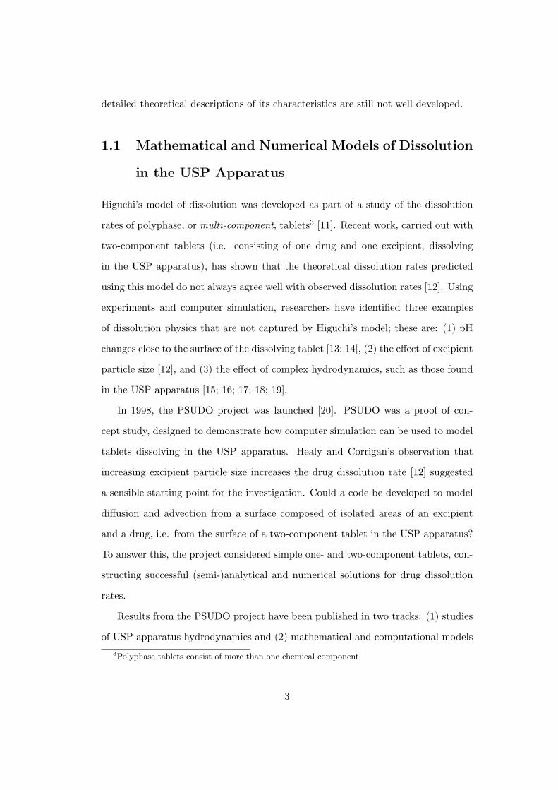
detailed theoretical descriptions of its characteristics are still not well developed.

1.1 Mathematical and Numerical Models of Dissolution

in the USP Apparatus

Higuchi’s model of dissolution was developed as part of a study of the dissolution

rates of polyphase, or multi-component, tablets3 [11]. Recent work, carried out with

two-component tablets (i.e. consisting of one drug and one excipient, dissolving

in the USP apparatus), has shown that the theoretical dissolution rates predicted

using this model do not always agree well with observed dissolution rates [12]. Using

experiments and computer simulation, researchers have identified three examples

of dissolution physics that are not captured by Higuchi’s model; these are: (1) pH

changes close to the surface of the dissolving tablet [13; 14], (2) the effect of excipient

particle size [12], and (3) the effect of complex hydrodynamics, such as those found

in the USP apparatus [15; 16; 17; 18; 19].

In 1998, the PSUDO project was launched [20]. PSUDO was a proof of con-

cept study, designed to demonstrate how computer simulation can be used to model

tablets dissolving in the USP apparatus. Healy and Corrigan’s observation that

increasing excipient particle size increases the drug dissolution rate [12] suggested

a sensible starting point for the investigation. Could a code be developed to model

diffusion and advection from a surface composed of isolated areas of an excipient

and a drug, i.e. from the surface of a two-component tablet in the USP apparatus?

To answer this, the project considered simple one- and two-component tablets, con-

structing successful (semi-)analytical and numerical solutions for drug dissolution

rates.

Results from the PSUDO project have been published in two tracks: (1) studies

of USP apparatus hydrodynamics and (2) mathematical and computational models

3Polyphase tablets consist of more than one chemical component.

3

of diffusion and advection. Taking as our starting point results from the second

track, described in [21; 17], the initial research question arrived at was, how can we

build on this work and improve our understanding of tablet dissolution in the USP

apparatus?

1.2 Thesis Aims

The aim of this work was to make progress in understanding drug dissolution in a

pharmaceutical test device. In vitro tests are critical to pharmaceutical development

yet their physics are not well understood. In what follows, the thesis that simulation

is useful for pharmaceutics is developed and argued through the presentation of three

main, separate investigations. These three distinct studies are connected to one

another in that they are inspired by the original problem of tablet dissolution in the

USP apparatus. Simulations of aspects of drug dissolution are of utility, not only as

isolated studies, but also as part of the development of a broader framework, which

includes previous and future work, for the simulation of pharmaceutical processes.

1.3 Thesis Structure

1.3.1 Study 1

In the first study, the starting point and core of the thesis, a Crank-Nicolson finite-

difference approximation to the drug mass transfer rate from dissolving cylindrical

tablets, consisting of alternating layers of drug and inert material, is presented. Re-

sults are compared with recent solutions to the same problem and with previous

experimental results produced using the USP apparatus. This first study is pre-

sented in Chapters 2 (literature review), 3 (theory and methods) and 6 (results and

discussion).

4

1.3.2 Study 2

The second study investigated the flow around the top of a cylinder using a com-

mercial fluid dynamics code. A specific application to a complementary problem in

wind energy is considered. In addition to other sources of error, accelerated airflow,

or speed-up, around the top of cylindrical meteorological (met) towers can cause

incorrect wind-speed measurements. A particular configuration is considered where

an anemometer, a device used to measure wind-speed, was located only 2 tower

diameters above a met tower.

The second study is presented in Chapters 4 (literature review, theory and meth-

ods) and 7 (results and discussion).

1.3.3 Study 3

The third part of this work considers one possible end state of a dissolving tablet:

fragmentation into small particles with dissolution continuing from the disintegrated

solid masses. A framework for calculating the motion of and dissolution from a drug

particle moving through the USP apparatus is outlined, beginning with a review of

the classical work of Taylor and Glauert, who considered the motion of raindrops in

airflows [22; 23].

The third study is presented in Chapters 5 (literature review, theory and meth-

ods) and 8 (results and discussion).

1.4 Summary

In the conclusion, this work is placed in context and the possibility of a complete

treatment of drug dissolution in the USP apparatus is discussed. The aim of this

work was to increase understanding of drug dissolution in the USP apparatus and

the three studies presented each represent an aspect of an overall solution. Most

importantly, however, the thesis presented is that simulation has significant potential

5

for pharmaceutics. The purpose of what follows is to demonstrate this to the reader.

1.5 Collaborators and Professional Acknowledgements

The work on flow about a cylindrical meteorological tower was completed in close

collaboration with Dimitri Perrin at the School of Computing in DCU and in part-

nership with INCA, the Institute for Numerical Computation and Analysis. Dimitri

deserves credit for much of the computational work completed for flows about hollow

towers of various configurations. Professor Michael Ryan of the School of Comput-

ing at DCU provided useful suggestions about how to proceed with the extension

of the Pohlhausen solution outlined. Susan Lazarus and Aongus O Cairbre at DIT

were also instrumental in arriving at extensions to the solution for exponents of

positive integers. Anne-Marie Healy and Deirdre D’Arcy of the School of Pharmacy

at Trinity College Dublin provided us with grid and velocity vector data from their

fluid dynamics simulation of the USP dissolution apparatus. Dr. Audrey Glauert

of Cambridge University kindly provided useful insight into the work of her mother,

Muriel Glauert.

1.6 Publications

1.6.1 Peer Reviewed Journals

Published papers produced from the work presented in this thesis are:

• N. McMahon, M. Crane, H. J. Ruskin and L. Crane, The Importance of

Boundary Conditions in the Simulation of Dissolution in the USP Apparatus.

Simulation Modelling Practice and Theory, Volume 15, Issue 3, March 2007,

Pages 247-255.

• D. Perrin, N. McMahon, M. Crane, H. J. Ruskin, L. Crane and B. Hur-

ley, The Effect of a Meteorological Tower on its Top-Mounted Anemometer.

6

Applied Energy, Volume 84, Issue 4, April 2007, Pages 413-424.

• N. McMahon, M. Crane, H. J. Ruskin and L. Crane, The Mechanics of

Drug Dissolution. 2003. Proceedings in Applied Mathematics and Mechanics

(PAMM), Volume 3, Issue 1, Pages 392 - 393.

1.6.2 Conference Oral Presentations

Work from this thesis was presented orally at two international conferences:

• Particle Tracking: from Raindrops in 1940 to Drug Dissolution in 2005. June

2005. Third M.I.T. Conference on Computational Fluid and Solid Mechanics.

MIT, Cambridge, MA.

• The Mechanics of Drug Dissolution. GAMM 2003. Abano-Terme (Padua),

Italy.

1.6.3 Conference Poster Presentations

Poster presentations of work from this thesis were prepared for two international

conferences:

• D. Perrin, L. Crane, N. McMahon and B. Hurley. The Influence of Mounting

Booms and Towers on Wind-Speed Measurements by Anemometers. Decem-

ber 2004. European Wind Energy Conference (EWEC), London.

• N. McMahon, M. Crane, H.J. Ruskin and L. Crane. Investigations into Tablet

Dissolution in a Paddle Type Apparatus. Polymers in Diffusion and Drug

Delivery 2003. Institute of Physics, London.

7

Chapter 2

Literature Review, Study 1

2.1 Introduction

A drug is a therapeutic or diagnostic entity and a drug delivery system (DDS) is

a system for delivering drugs into the body [24]. Pharmaceutics is concerned with

designing drugs and their delivery systems [7]. Two decades ago, the disciplines that

contributed to pharmaceutics included chemistry (analytical, medicinal and biolog-

ical), pharmacology (the study of the effect of drugs on organisms), toxicology and

clinical medicine [25]. Today, new technologies and better theoretical understanding,

drawing from disciplines such as applied mathematics, engineering and especially

computing, have broadened the scope of pharmaceutics to include bioengineering,

computer simulation, computational biology and bioinformatics, genomics and struc-

tural genomics, all of which can be classed as biotechnologies [26; 27; 28; 29]. Small

biotechnology companies, many of them 21st century start-ups, have rapidly estab-

lished themselves as the innovators of the pharmaceutical industry, bringing ideas

from academia to the factory [27].

8

2.1.1 Drug Delivery Systems

Controlled Drug Delivery Systems

Drug delivery systems, specifially controlled drug delivery systems, are designed to

deliver a drug with precision [30]. There are three main categories of controlled

drug delivery systems, (i) controlled release delivery systems, (ii) localised delivery

systems and (iii) targeted delivery systems [31]. Localised systems attempt to con-

fine the drug to an organ or space in the body, while targeted systems affect only

particular cell types, e.g. cancer cells.

Controlled-release systems deliver drugs at a predetermined rate appropriate to

the disease, maximising the drug’s effectiveness while minimising the risk of over-

dose and toxic effects [32; 28]. Controlled-release systems are important for treating

illnesses such as diabetes, where precise delivery with time is critical and undesir-

able effects1 can be fatal. Controlled-release systems can also eliminate unpleasant

administration methods such as parenteral delivery (injections) and increase patient

compliance and comfort [33].

In the 1950s, Smith Kline & French introduced the first controlled-release medicine,

Dexedrine, in a device the company called a Spansule [34]. It quickly released the

required initial dose and then slowly and gradually released many extremely small

doses to maintain a therapeutic level lasting from 10 to 12 hours [35]. This was

achieved by using between two and eight groups of drug pellets, each group coated

with a different thickness of slowly dissolving inert material. The spansule used the

dissolution characteristics of the drug and coating to control the drug release.

Diffusion- and dissolution-controlled systems can be classified broadly as primar-

ily subject to either bulk erosion or surface erosion, although other advanced devices

also exist including implantable microchips with onboard drug reservoirs [28]. By

bulk erosion is meant that drug mass is lost uniformly throughout the system. Ero-

1Such effects include dose dumping, the rapid release of drug at a rate that quickly leads to toxiclevels of drug in the bloodstream [3].

9

Figure 2.1: Smith Kline & French’s controlled release Spansule delivery system.Drug delivery is regulated with pellets coated with varying thicknesses of a slowlydissolving material. Reproduced from [35].

sion rates depend on the volume of the compact. Surface eroding systems erode

from the outside to the inside of the system and the erosion rate depends on the

surface area of drug exposed [32]. The spansule system depended on surface erosion

(Figure 2.2).

The dissolution rate of drug from a delivery system can be classed as [7]:

• Zero Order :dc

dt= −k. In this case, the dissolution rate of a drug is constant,

k, and independent of its concentration in the solution, c. The solution to this

equation is the linear equation, c = C0 − kt, where C0 is the concentration at

time t = 0.

• First Order :dc

dt= −kc; where the dissolution rate depends linearly on c. The

solution can be written as a linear equation in the form lnc = lnC0 − kt.

• Second Order :dc

dt= −kc2; where the dissolution rate depends on c2. The

solution to the second order release equation can be written as a linear equation

in the form1

c=

1

C0

+ kt.

With zero order, or constant rate, delivery systems, a uniform concentration of

drug is always available for absorption within a defined therapeutic window [36]. A

zero order drug release profile is the primary aim when designing controlled release

10

1.0

0.5

01.00.750.50.250

Con

cent

ratio

n

Time

(a)

1.0

0.5

0.250.3750.250.1250

Con

cent

ratio

n

Time

(b)

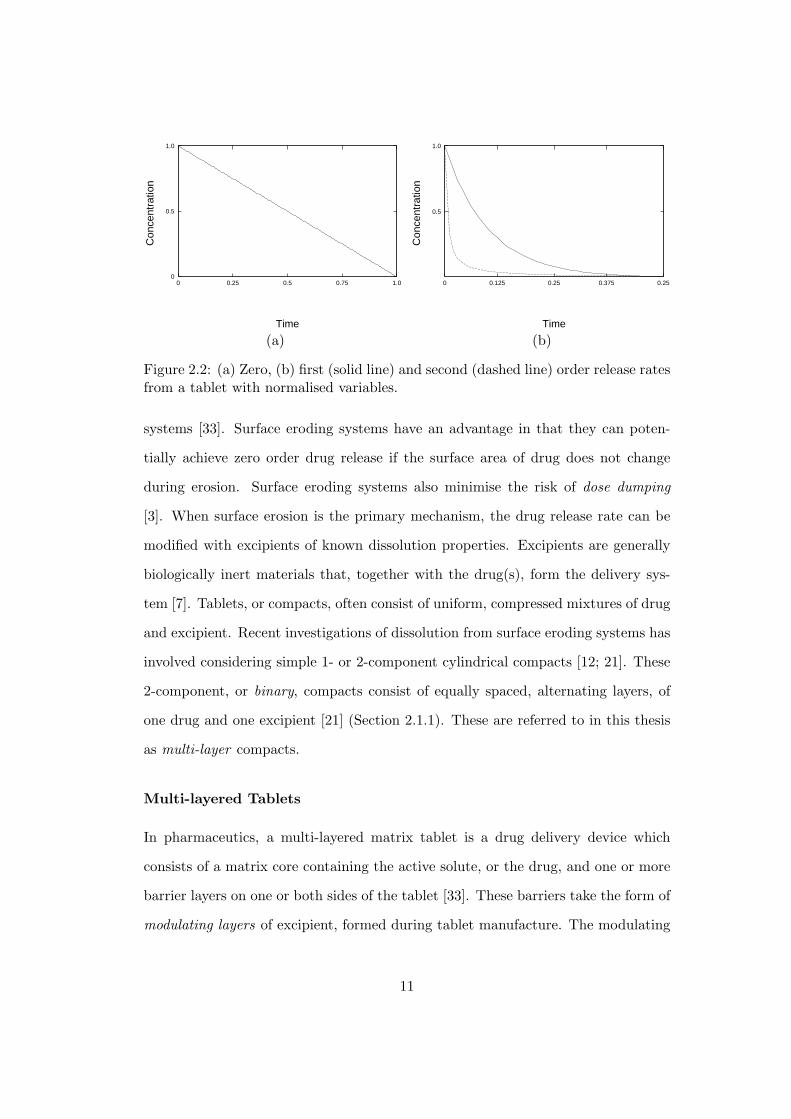
Figure 2.2: (a) Zero, (b) first (solid line) and second (dashed line) order release ratesfrom a tablet with normalised variables.

systems [33]. Surface eroding systems have an advantage in that they can poten-

tially achieve zero order drug release if the surface area of drug does not change

during erosion. Surface eroding systems also minimise the risk of dose dumping

[3]. When surface erosion is the primary mechanism, the drug release rate can be

modified with excipients of known dissolution properties. Excipients are generally

biologically inert materials that, together with the drug(s), form the delivery sys-

tem [7]. Tablets, or compacts, often consist of uniform, compressed mixtures of drug

and excipient. Recent investigations of dissolution from surface eroding systems has

involved considering simple 1- or 2-component cylindrical compacts [12; 21]. These

2-component, or binary, compacts consist of equally spaced, alternating layers, of

one drug and one excipient [21] (Section 2.1.1). These are referred to in this thesis

as multi-layer compacts.

Multi-layered Tablets

In pharmaceutics, a multi-layered matrix tablet is a drug delivery device which

consists of a matrix core containing the active solute, or the drug, and one or more

barrier layers on one or both sides of the tablet [33]. These barriers take the form of

modulating layers of excipient, formed during tablet manufacture. The modulating

11

Figure 2.3: The difference between surface and bulk erosion. Black denotes a highconcentration of drug. Reprinted from [37], Copyright (2001), with permission fromElsevier.

layers slow the interaction of the drug and the solvent by (i) limiting the surface area

of solute exposed to the solvent and (ii) controlling the penetration rate of solvent

into the matrix core. Modulation layers extend the time it takes for the drug to

dissolve, preventing dose dumping, and lead to linear, or zero-order, dissolution

rates [38; 39; 36; 33].

Layered compacts are uncommon in practice, though similar devices have been

proposed as viable delivery systems. Conventional matrix tablets containing drugs

are generally not zero-order, the release rate falls continuously with time [38]. Al-

though multi-layer systems usually attempt to achieve a zero-order release rate, some

multi-layer systems have been designed to achieve bimodal release [38]. Bimodal re-

lease consists of an initial rapid release of drug followed by a constant release phase

and a second period of rapid release [38].

The state of the art in multi-layered tablet design includes zero-order release

sustained systems, quick/slow systems, time-programmed systems and bimodal sys-

12

tems [33]. A 3-layer tablet architecture that achieves near zero-order release is

outlined by Qiu et al. [40]. The middle layer contains the active drug. This is

sandwiched between water-soluble or water-insoluble barrier layers. Geomatrix is a

well known patented multi-layer delivery system [41]. Based on work carried out at

the University of Pavia in the 1980s, Geomatrix is licensed by SkyePharma and is

used by companies including Sanofi-Aventis [42]. Geomatrix is designed to deliver

a constant rate of drug when in the stomach and the intestines. In addition to

achieving near zero-order performance, multi-layer systems have the advantage of

low-cost and ease of manufacture [33].

2.1.2 Dissolution Testing

Dissolution testing has evolved over the past three decades to become a critical com-

ponent of pharmaceutical R&D and manufacturing [7; 9]. Broadly speaking, there

are three main reasons for carrying out dissolution tests: (i) to ensure consistency of

output during manufacture, (ii) to assess the factors affecting the bioavailability of

the drug and (iii) to make predictions about the performance of the delivery system

in vivo. It is thus an important test from a clinical perspective [9].

In general, a drug must be in the form of a solution for absorption across the

membranes of the gastrointestinal tract into the circulatory system [43; 7]; this

means that the design of new formulations and specifications are often guided by in

vitro dissolution tests which mimic conditions in the GI tract, e.g. USP dissolution

apparatus [44; 18]. The effect of changing formulation and manufacturing process

variables can be assessed with dissolution testing [7].

In making in vivo claims based on in vitro data, it is important that an in vitro

in vivo correlation (or IVIVC) is clearly established [8]. In vitro in vivo correlation

in this sense refers to the relationship between the in vitro dissolution of the drug

in the test apparatus and the release or absorption of the drug in vivo, in a patient

[7]. In vitro dissolution tests certainly capture some of the physics of in vivo ab-

13

Figure 2.4: Multi-layered matrix tablets. Reprinted from [33], Copyright (2004),with permission from Elsevier.

14

sorption, in that, for example, the USP defined dissolution apparatus can contain a

stirred solution of 0.1M HCl, approximating stomach conditions. Although dissolu-

tion tests have developed primarily as manufacturing quality controls and to guide

the development of new delivery systems, not as simulations of in vivo delivery [7],

it is possible to state with confidence that dissolution tests do indicate if the de-

livery system disintegrates correctly [9]. In addition, the availability of a drug for

gastrointestinal absorption from solid dosage forms is often reflected by the in vitro

dissolution rate [45]. However, dissolution tests can only be used to generate in

vitro /in vivo correlations (and possibly as in vivo surrogates) under strictly defined

conditions [8].

Recent analyses of the USP standard dissolution apparatus have indicated in-

trinsic variability in its operation: the extent to which in vivo absorption can be

correlated with in vitro drug dissolution standard testing devices is not at all certain

[15; 18] and it can therefore be difficult to build consistent correlations.

This variability also has serious implications for quality assurance on pharma-

ceutical production lines. One of the more common dissolution testing devices is the

USP Type 2 Paddle Dissolution Apparatus [10], i.e. the USP apparatus referred to

throughout this document. This consists of a covered transparent vessel, made of

an inert material and filled with a dissolution medium (Figure 2.5). The compact

is placed at the bottom of the device. Water is generally used as the dissolution

medium but other media may be used as specified by the pharmacopeia, e.g. dilute

HCl. The vessel is cylindrical with a hemispherical bottom and a paddle is used to

stir the dissolution medium at constant rate as specified by the USP. The tempera-

ture inside the vessel is maintained at 37 ± 0.5 by placing the vessel in a water

bath or using a heating jacket.

15

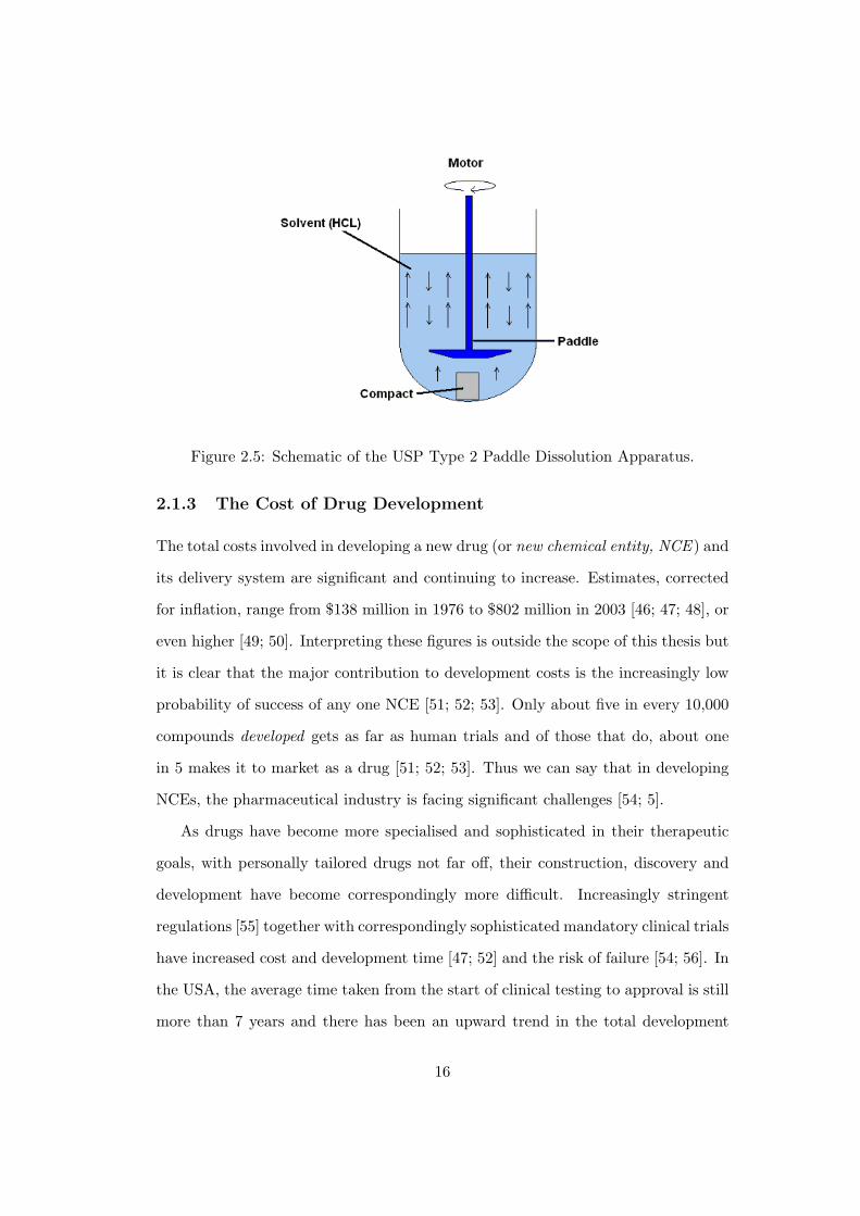
Figure 2.5: Schematic of the USP Type 2 Paddle Dissolution Apparatus.

2.1.3 The Cost of Drug Development

The total costs involved in developing a new drug (or new chemical entity, NCE ) and

its delivery system are significant and continuing to increase. Estimates, corrected

for inflation, range from $138 million in 1976 to $802 million in 2003 [46; 47; 48], or

even higher [49; 50]. Interpreting these figures is outside the scope of this thesis but

it is clear that the major contribution to development costs is the increasingly low

probability of success of any one NCE [51; 52; 53]. Only about five in every 10,000

compounds developed gets as far as human trials and of those that do, about one

in 5 makes it to market as a drug [51; 52; 53]. Thus we can say that in developing

NCEs, the pharmaceutical industry is facing significant challenges [54; 5].

As drugs have become more specialised and sophisticated in their therapeutic

goals, with personally tailored drugs not far off, their construction, discovery and

development have become correspondingly more difficult. Increasingly stringent

regulations [55] together with correspondingly sophisticated mandatory clinical trials

have increased cost and development time [47; 52] and the risk of failure [54; 56]. In

the USA, the average time taken from the start of clinical testing to approval is still

more than 7 years and there has been an upward trend in the total development

16

time from NCE discovery to DDS approval since the 1960s [47]. In 2005, it was

between 12 and 15 years [53]. Problems that appear at the end of clinical testing

can seriously damage a company’s finances [54] [e.g. GTC Biotherapeutics’s Atryn

and Elan’s Tysabri 57; 58; 59; 60].

The increasing financial cost of drug development is a function of (1) techni-

cal uncertainty, (2) regulatory uncertainty and (3) market uncertainty [47]2. The

promising NCE must be discovered, understood and developed into an effective

DDS, it must be safe and, most importantly, it must be in demand.

Aspects of the pharmaceutical development process are also costed using ethical

rather than economic measures. In vivo animal trials are presently necessary but

undesirable [61] and provoke controversy [62]. There is a consensus that the refine-

ment, reduction and eventual replacement of animals in pharmaceutical research are

pursuits of critical importance [63; 64]. Indeed, they are central tenets of the health

strand of the EU’s Seventh Framework Programme for Research [65].

The priority for modern pharmaceutical companies is therefore to control costs,

measured both economically and ethically, while maintaining standards [46; 54].

2.1.4 Simulation and Pharmaceutics

In 1975, Chapman, Mark and Pirtle [66; 67] laid down three practical aspirations

for simulation in aerospace, namely to provide flow simulations that are impossible

to produce using wind tunnel tests or other experiments, to cut the time and cost

of building flow simulations and to provide more accurate flight simulations than

wind tunnels can. Since then, the aerospace industry has embraced simulation [68].

Adapting the motivations for adopting computational fluid dynamics [66; 69; 70]

to pharmaceutics, we can write that computer simulation: (1) reduces research and

development lead-times, (2) can investigate pharmacokinetic mechanisms not easily

reproducible in experimental models, (3) can provide more detailed and compre-

2In recent years, litigation costs have also added to the overall cost of drug development. Thefailure of prospective drugs during clinical trials, however, remains the single biggest factor.

17

hensive information, (4) could reduce all costs and (5) could be more efficient than

experimental testing. The use of simulation in drug development has the potential

to yield more successful products, fewer failures and faster time to market [6].

Computer simulation may have an impact on all aspects of pharmaceutics, from

discovery through to final clinical testing [71]. With the completion of the human

genome project and the explosion in bioinformatics technology, the number of molec-

ular targets for drugs is expected to jump from approximately 500, in 2003, to many

thousands within a few years; in addition, the analysis of the human genome is ex-

pected to eventually speed drug development [72; 4]. With better understanding,

the number of drug candidates for a particular target can be optimised in silico for

high-throughput physical screening. Multivariate statistical computer simulations

can help in the design of clinical tests, to predict the results of clinical studies and

identify those with a satisfactory probability of success [73]. Simulations of drug

delivery devices could predict the effect of changing process or formulation variables

on the resulting drug release profile [37; 74].

Although many simulation companies have concentrated efforts on drug discov-

ery tools, there are some working on physiologically based pharmacokinetic (PBPK)

simulation [75; 76; 77]. An example of this is the Israeli firm Optimata which has

conducted clinical trials at Nottingham City Hospital in Britain and Soroka Med-

ical Center in Negev of a simulation tool used to optimise therapeutic regimes for

cancer patients [78]. Optimata has already successfully modelled protocols for drug

delivery in animals [79].

The convergence of computing and engineering capability, the need for pharma-

ceutical companies to reduce R&D risks, and an acceptance of the interdisciplinary

nature of pharmaceutics by pharmacists and biologists are all contributing to the

growing importance of simulation [80; 81]. About half of the top 40 pharmaceutical

companies are using simulation and modelling tools [4]. According to extrapolated

possible scenarios, by 2015 computer modelling and simulation will be core to drug

18

development [4; 5].

Russell and Burch outlined benchmarks for the ethical, legal and scientific use of

animals in research and development, introducing the idea of the 3 Rs: replacement,

reduction and refinement [61; 82; 83; 64]. Our understanding of the body at all levels

is improving continuously [6]. At one extreme of our understanding are results from

the human genome sequencing project [84]. At the other extreme, researchers are

constructing models of complete organs [85]. IBM’s Blue Gene project has as one

of its main objectives the application of Blue Gene’s computational resources to

significant scientific problems and the project has identified protein folding as its first

challenge [86]. The combination of constantly improving theoretical understanding

and computing technology is allowing an increasingly large number of processes to

be simulated at all levels of biological organisation; this may culminate in models

of the human body that, for all required purposes, are in silico human systems.

At the very least, computer simulation has the potential to reduce the need for

experimental testing, both in vitro and in vivo testing.

2.2 Drug Dissolution Modelling

The theory of dissolution has been studied for over a century and it is a century since

it was established that dissolution takes place in two stages [87; 88]. The first is the

separation of drug molecules from the surface of the solid to form a solution saturated

with drug at the solid-liquid interface. In practice, this is achieved by maintaining

the concentration of drug in the solid to be very much higher than the drug solubility

[32]. The second stage is the mass transport of the drug from this saturated layer

into the bulk solution [88]. This second stage has most influence on the dissolution

process. In general, the mass transport is the result of two mechanisms, diffusion

and convection, described by the concentration boundary-layer equations3.

3The concentration boundary-layer is a thin layer of fluid in the immediate vicinity of a diffusingsurface where the concentration gradient normal to the surface is very large [89].

19

2.2.1 Classical Work

Noyes and Whitney

The original and most famous model was developed over a century ago by Noyes

and Whitney [87]. Based on observation of two quite different materials dissolving

in distilled water, Noyes and Whitney deduced the general law:

∂c

∂t= k(Cs − c) (2.1)

where Cs is the solubility of the substance, or the concentration of its saturated

solution; c is the concentration after a time t, and k is a constant of proportionality.

Integrating this equation with appropriate assumptions gives:

k =1

tln

Cs

(Cs − c)(2.2)

Noyes and Whitney obtained values for the solubility Cs and the concentration c

for several values of t. With these values and Equation (2.1), values for the constant

k were determined for benzoic acid and lead chloride dissolving in distilled water.

As they revealed, k remains constant for a particular binary system of a solute

A and solvent B.

Nernst and Brunner

The work of Noyes and Whitney was later modified by Nernst and Brunner [90; 91].

Nernst and Brunner proposed the two-stage dissolution process that still has cur-

rency today [88; 20]. They observed that during dissolution, (i) the layer of solution

at the solid-liquid interface reaches saturation concentration almost immediately, af-

ter which (ii) diffusion takes place across the diffusion layer. In addition, Nernst and

Brunner assumed that the fluid in this diffusion layer was stagnant. Although this

model is very useful, later work showed that these assumptions are not necessary

20

[92]. The processes at the solid-liquid interface do not need to be instantaneous,

only rapid relative to the processes in the diffusion layer. In addition, the fluid in

the diffusion layer does not need to be stagnant. Under many practical conditions,

such as those found in the USP dissolution apparatus, this assumption is unrealistic.

The diffusion layer can have both velocity and concentration profiles normal to the

surface. This is an expression of the concept of the boundary-layer [93; 89]. Never-

theless, the models of Noyes and Whitney and Nernst and Brunner do yield useful

results for sink conditions, i.e. if the concentration of the solute never exceeds 10%

of Cs [87; 92; 88].

The Noyes-Whitney equation for sink conditions is generally written in the form:

dm

dt=DACs

h(2.3)

wheredm

dtis the mass transfer rate, and the constant of proportionality C is

replaced withDA whereD is the diffusion coefficient, generally defined as a quantity

having the units [m]2[s]−1, h is the effective diffusion layer thickness and A is the

surface area available for dissolution [94; 7].

Higuchi

Higuchi’s model was developed as part of a study of the dissolution rates of multi-

component, or polyphase, tablets where the dissolving crystalline components A and

B form an intimate, uniform, non-disintegrating mixture and are assumed not to

interact with one another [11].

Higuchi observed that, when exposed to a solvent, the dissolution rates of the

two components can be described in the initial stages by the Noyes-Whitney model.

After a short period of time, however, one of the phases will be depleted at the

solid-liquid interface. This is because the ratio of the diffusion-controlled dissolution

rates of the two components (DAC0A/DBC

0B) is not proportional to the ratio of the

amount, or mass, of each component (NA/NB) originally in the mixture at the

21

surface, i.e. one component may dissolve faster than the other. DA and DB are the

dissolution coefficients of A and B in the solvent respectively and C0A and C0

B are

the solubilities of A and B. After a time t1, a thin layer extending to just below

the surface will consist of only one of the components. Aside from the exceptional

critical situation (when NA/NB = DAC0A/DBC

0B), the thin layer will consist entirely

of either A or B after a time t1; these, Higuchi called situations A and B respectively.

Taking situation A, when the surface is purely made up of component A after a

time t1, Higuchi defines two important positions, S1 and S2. S1 is the solid-liquid

interface at the surface, while S2 is the interface between the bulk solid mixture and

the solid phase A layer just inside the surface. ∆S = S2 − S1. Since A is at the

surface, the dissolution rate of A is given as:

GA =DAC

0A

h(2.4)

where h is the effective diffusion layer thickness. What Higuchi calls the mass

dissolution rate GA, therefore, is in fact the dissolution rate per unit surface area

or the mass flux.

Molecules of B, however, must pass through not only the diffusion layer thickness

h, but also through the solid layer of phase A, of thickness ∆S. Higuchi then writes

the mass flux of component B from the surface as

GB =DBC

0B

h+ τǫ∆S

=NB

NAGA (2.5)

where τ and ǫ are the tortuosity and porosity of the solid phase A respectively.

The porosity is a measure of how well packed the solid is or how much empty

space between component particles exists4 while the tortuosity is a measure of the

increase in distance a diffusing molecule travels due to bending and branching of

4In pharmacy, porosity can be defined as a function of the ratio between the apparent and true

densities of a tablet, i.e. ǫ = 1 −

ǫapparent

ǫtrue

[95].

22

pores between voids in the solid components [95; 96]5. τ and ǫ are usually expressed

as dimensionless ratios or percentages [7].

Equations (2.4) and (2.5) are valid for steady-state sink conditions and when

no phase B remains in solution within the pores of the thin A phase layer. This

is true for most practical situations. These equations, along with similar equations

for the reverse situation when A dissolves faster than B, were used by Higuchi to

predict the dissolution from discs of benzoic and salicylic acid dissolving in 0.1M

HCl. His results matched well for many systems and Higuchi’s model is still relevant

and useful today.

2.2.2 Contemporary Work

Recent work, carried out with two-component tablets, i.e. consisting of one drug

and one excipient, dissolving in the USP apparatus, has shown that the theoreti-

cal dissolution rates predicted using Higuchi’s model do not always agree well with

observed dissolution rates. Researchers, using experiments and computer simula-

tion, have identified three examples of dissolution physics that are not captured by

Higuchi’s model. These are: (1) pH changes close to the surface of the dissolving

tablet [13; 14], (2) the effect of excipient particle size [12; 97; 98], (3) complex hy-

drodynamics, such as those found in the USP apparatus [15; 16; 17; 18; 19]. The

effect of particle size was particularly interesting; large particles of fast-dissolving

excipient seem to increase the drug dissolution rate. One explanation is that, once

dissolved, large particles leave behind large pores on the compact surface, increas-

ing the effective surface area of drug exposed to the solvent for all values of drug

loading. This mechanism is, however, not well understood.

Nevertheless, this explanation suggested theoretical and experimental investiga-

tions of how drug and excipient dissolution properties affect the surface area of drug

5Tortuosity is normally defined as the ratio of the actual path length through the pores to the

Euclidean, or shortest, distance, i.e. τ =Eactual

EEuclid.

. A straight pore has a tortuosity of exactly one,

expressed as a ratio [96].

23

Figure 2.6: An idealised multi-layer compact.

and its delivery rate during dissolution [21]. To this end, recent work has involved

modelling simple one or two component cylindrical compacts, dissolving in the USP

dissolution apparatus. The two component compacts consist of equally spaced al-

ternating layers of one drug and one excipient. These idealised multi-layer compacts

are referred to as simply multi-layer compacts in the remainder of this thesis.

Researchers chose the multi-layer configuration for reasons including: (i) it is

a simple starting point, with well-defined regions of drug and excipient [21], (ii)

techniques used to model this system may be applied to uniformly mixed multi-

component compacts [20] and (iii) a multi-layer code had already been written [99].

The PSUDO Project

The PSUDO6 proof of concept project, initiated in 1998, demonstrated how com-

puter simulation can be used to model compacts dissolving in the USP apparatus

[100; 20]. This project followed on from earlier investigations in Trinity College

Dublin into the validity of Higuchi’s Model [14; 99; 12].

The PSUDO project focused on understanding and modelling multi-component

compacts dissolving in the USP apparatus. The numerical code was based on a fi-

nite element model [99]. During the course of the project, experiments showed that

the hydrodynamic conditions in the device were complex, confirming work from the

6Parallel SimUlation of Drug release cOde. Funded by the European Union Fourth FrameworkProgramme for Research. PSUDO was a collaboration between Hitachi, Elan and the Schools ofPharmacy and Mathematics at Trinity.

24

1990s [14; 12]. The project concluded in 2000 and was considered a qualified success,

falling short of its target to fully model two component dissolution but demonstrat-

ing reasonable agreement between in silico and in vitro results for single component

compacts and initial multi-component investigations [20]. In the final report, phar-

macists from Elan and Trinity noted that experimental and numerical results for a

single component were in reasonable agreement but that there was still work to be

done for two-component systems and in considering the complicated flow patterns

in the USP apparatus [20]. The project concluded with a road-map for future work:

to continue the development of the mathematical models (for application to more

complicated systems) and to investigate the hydrodynamics of the test apparatus,

eventually integrating the dissolution and hydrodynamic models to produce a model

of the test apparatus.

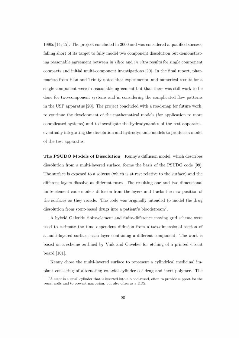
The PSUDO Models of Dissolution Kenny’s diffusion model, which describes

dissolution from a multi-layered surface, forms the basis of the PSUDO code [99].

The surface is exposed to a solvent (which is at rest relative to the surface) and the

different layers dissolve at different rates. The resulting one and two-dimensional

finite-element code models diffusion from the layers and tracks the new position of

the surfaces as they recede. The code was originally intended to model the drug

dissolution from stent-based drugs into a patient’s bloodstream7.

A hybrid Galerkin finite-element and finite-difference moving grid scheme were

used to estimate the time dependent diffusion from a two-dimensional section of

a multi-layered surface, each layer containing a different component. The work is

based on a scheme outlined by Vuik and Cuvelier for etching of a printed circuit

board [101].

Kenny chose the multi-layered surface to represent a cylindrical medicinal im-

plant consisting of alternating co-axial cylinders of drug and inert polymer. The

7A stent is a small cylinder that is inserted into a blood-vessel, often to provide support for thevessel walls and to prevent narrowing, but also often as a DDS.

25

Figure 2.7: A schematic of Kenny’s code. The code solves for the situation of purediffusion in the region next to a dissolving surface.

core code was subsequently successfully adapted by the PSUDO project for diffu-

sion from multi-layer compacts standing vertically in a USP apparatus with the aim

of extending the solution to account for advective mass transfer, resulting in a code

that captured diffusion, advection and the receding drug/fluid interface [20]. In

order to achieve this, additional code was wrapped around the code from Kenny’s

work. Three different wrappers, or methods, were described and are outlined below.

The first solution outlined involved solving a simplified cylindrical formulation

of the advection-diffusion equation [20; 102]

∂c

∂t= −vz

∂c

∂z+D

(

∂2c

∂r2+

1

r

∂c

∂r+∂2c

∂z2

)

(2.6)

where c is the concentration, vz is the velocity in the z direction, parallel to

the surface, D is the dissolution coefficient and r is the displacement in the radial

direction, i.e. normal to the surface. It can be read that the change in concentration

with time in a given point volume in the fluid is equal to the net amount of material

advected into the volume in unit time in the z (streamwise) direction plus the net

amount of material diffused into the volume in both directions in unit time. This

represents Kenny’s original code with a simplified advection term added (see Figures

2.7 and 2.8).

In this instance, the fluid velocity vz is assumed to be constant at all distances

from the surface and mass is only advected parallel to the surface. At every point,

26

Figure 2.8: A schematic of Method 1 in the PSUDO code. The code solves for thesituation of pure diffusion as well as simplified advection in the region next to adissolving surface.

the change in concentration with time is assumed to consist of the net change in

concentration due to diffusion plus the net change in concentration due to advection

in the z-direction.

In the second model proposed by the PSUDO team, the problem is simulated as

pure diffusion in the region next to the surface (Figure 2.9). To capture advection,

a convective boundary condition is used on the boundary between the diffusion

layer and the rest of the fluid. The convective boundary condition depends on the

free-stream velocity and takes the form

D∂c

∂n

∣

∣

∣

∣

n=0

= −hm(Cs − Cbulk) (2.7)

where Cbulk is the concentration of the drug in the bulk fluid, hm is the convection

mass transfer coefficient and n is the displacement normal to the surface, with the

other quantities already defined [20; 102]. As in Method 1, the free-stream velocity

vz is again assumed to be constant and is given as an input.

The mass of drug in the solution at t = t + ∆t is then calculated using the

formula

m(t+ ∆t) = m(∆t) + ∆t

∫

Γ

vn(c− Cbulk)dΓ +

∫

Ω

cdΩ (2.8)

which can be read as the amount of drug in the simulation domain at time t +

27

Figure 2.9: A schematic of Method 2 in the PSUDO code. The code solves for thesituation of pure diffusion in the region next to a dissolving surface. Advection iscaptured by imposing a convective boundary condition on the upper boundary ofthe diffusion layer.

the amount of drug convected across the boundary Γ between the diffusion region

and the bulk region + the amount of drug in the diffusion region (Ω). The steps in

calculating the mass transfer rate are:

1. Set Cboundary = advective boundary condition

2. Run diffusion simulation and calculate flux from surface

3. Assume the advective flux is the same as the surface flux (because of mass

continuity)

4. Calculate the amount of mass advected into fluid in ∆t

5. Recalculate Cbulk and iterate

The third PSUDO method also assumes pure diffusion in the region close to

the surface (Figure 2.10). It is assumed that the concentration c at the freestream

boundary of this region is equal to cbulk. The increase in mass of drug in the volume

outside the layer in unit time is then set equal to

m(t+ ∆t) = m(t) + ∆t

∫

Γ

vz(c− Cbulk)dΓ (2.9)

28

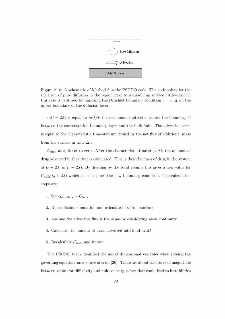
Figure 2.10: A schematic of Method 3 in the PSUDO code. The code solves for thesituation of pure diffusion in the region next to a dissolving surface. Advection inthis case is captured by imposing the Dirichlet boundary condition c = cbulk on theupper boundary of the diffusion layer.

m(t + ∆t) is equal to m(t)+ the net amount advected across the boundary Γ

between the concentration boundary-layer and the bulk fluid. The advection term

is equal to the characteristic time-step multiplied by the net flux of additional mass

from the surface in time ∆t.

Cbulk at t0 is set to zero. After the characteristic time-step ∆t, the amount of

drug advected in that time is calculated. This is then the mass of drug in the system

at t0 + ∆t, m(t0 + ∆t). By dividing by the total volume this gives a new value for

Cbulk(t0 + ∆t) which then becomes the new boundary condition. The calculation

steps are:

1. Set cboundary = Cbulk

2. Run diffusion simulation and calculate flux from surface

3. Assume the advective flux is the same by considering mass continuity

4. Calculate the amount of mass advected into fluid in ∆t

5. Recalculate Cbulk and iterate

The PSUDO team identified the use of dimensional variables when solving the

governing equations as a source of error [20]. There are about six orders of magnitude

between values for diffusivity and fluid velocity, a fact that could lead to instabilities

29

when fine grids or time-steps are used. Other problems included difficulty with the

definition of boundary conditions, such as how to impose fixed conditions and how

to implement moving boundary conditions, e.g. setting the bulk concentration. A

new analysis carried out for this thesis, considering the effect of fluid velocity on the

overall error, is presented in the Results and Discussion Section.

Outcomes of the Project Papers, based on work carried out during the PSUDO

project, were subsequently published in two distinct tracks. These tracks have

proceeded in parallel, but with collaboration, over the past five years.

Following on and adding to the work of experimenters in the 1990s, the PSUDO

project prompted an investigation into the hydrodynamics of the USP apparatus

[17]. Although the dissolution test is widely used, high variability in results have

been reported and its fluid dynamics are for the most part not well understood

[15]. Dissolution test failures have led to many product recalls and inconsistencies

and variability in test results are a significant problem8 [18]. The dissolution test

is a highly variable technique; the major sources of variability are the geometric

parameters of the device and the stirring mechanism, both leading to complex hy-

drodynamics [15]. Surface imperfections in the vessel can also lead to variability in

the results [103].

Contemporary computational fluid dynamics (CFD) simulations [104; 105; 44;

16; 18; 19] have shown that the flow field in the device is fully three-dimensional

and that small displacements of the compact can lead to significant changes in the

dissolution rate of the dosage form. Increasing the stirring speed of the dissolution

apparatus to about 200 rpm results in a higher, non-linear, drug release rate [98].

These studies strengthen the argument that it is the intrinsically complex hydro-

dynamics of the device that cause most of the variability in dissolution test results

[18].

816 % of non-manufacturing recalls of solid oral dosage forms in the period 2000-02 were due totest failures .

30

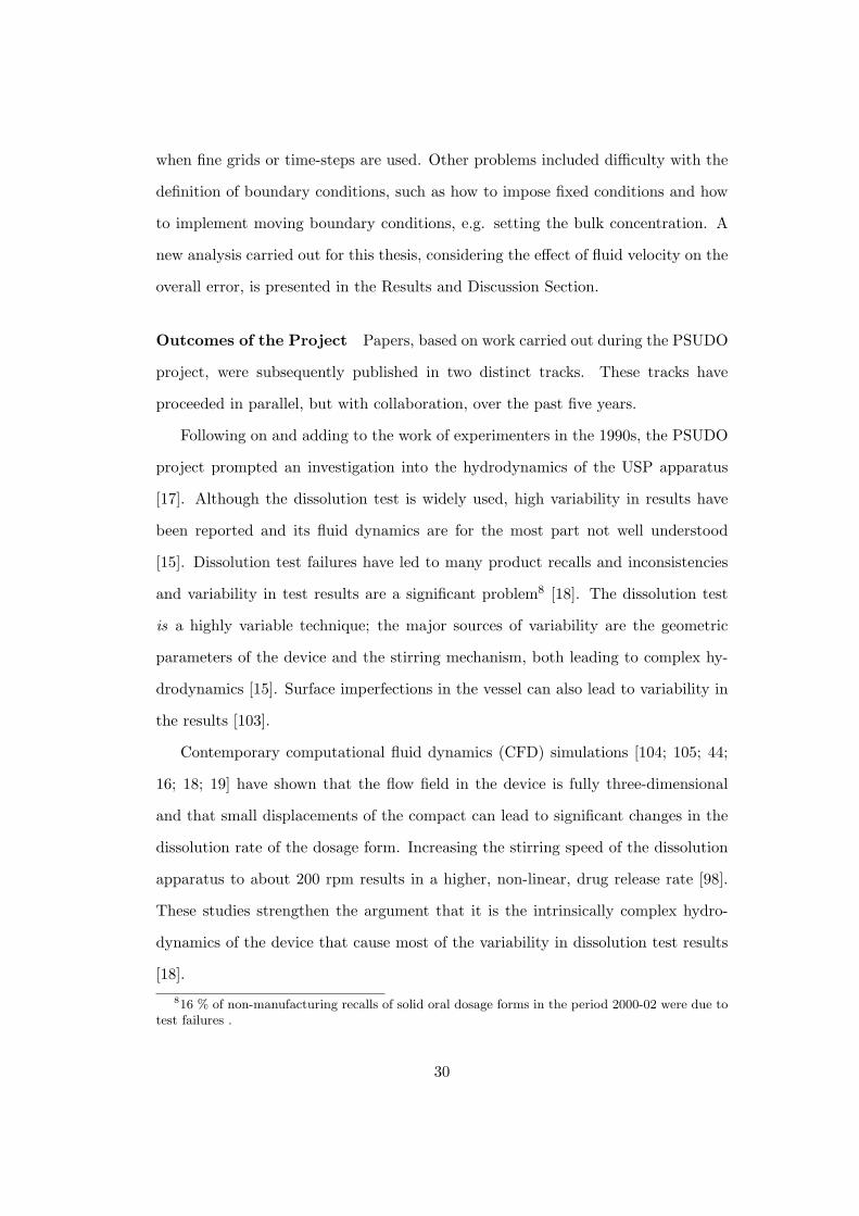
Figure 2.11: Section from the 3D USP hydrodynamic simulation built by [19] usingthe commercial code Fluent. The computational mesh is shown on the left withcomputed velocity magnitudes on the right.

Accepting, then, that much of the variability in results is attributable to the

complex and heterogenous hydrodynamics of the device, an important question is

raised: to what extent are these complex hydrodynamics a function of factors that

we can control, and to what extent are they intrinsic to the design of the USP

apparatus [17]? Two research teams have worked in the area of USP hydrodynamics

over the past number of years. Healy, McCarthy, Corrigan, D’Arcy and others,

following on from the PSUDO project, have built Fluent9 CFD simulations of the

USP apparatus, investigating the sensitivity of the results to the location of the

compact in the device [104], comparing the simulated flow of the bulk fluid with

laser doppler measurements [105], examining the flow patterns next to a compact

placed centrally at the bottom of the device [44] and the dissolution from compacts

at various positions on the bottom of the device [19]. Kukura, Baxter, Muzzio

and others have completed simulations and experimental studies similar to those of

9The commercial computational fluid dynamics code [106].

31

Healy et al [e.g. 104]. These include studies of the hydrodynamics and shear within

the device [16] and the variability of dissolution with position in the device [18]. All

these studies conclude that the complex heterogeneous hydrodynamic environment

within the USP apparatus leads to the observed variability in the test and that the

hydrodynamics are intrinsic to the design of the USP Type 2 Dissolution Apparatus.

The second track, indicated by PSUDO, involves improving the analytical and

numerical models of mass transfer [e.g. 21; 17]. The work presented in this thesis

follows on from this track. As outlined in Chapter 1, the questions that are raised

include: how can we build on this work and improve our understanding of tablet dis-

solution in the USP apparatus? Can we generalise the analytical solution described

by Crane et al. [21]? Can we determine the validity of this analytical solution? Can

we build a better numerical solution? Can we say anything about the end phase of

tablet dissolution?

Crane, Hurley et al.

As one of the publications generated by the PSUDO project, Hurley and Crane

present analytical and numerical solutions for the mass transfer from simple 1-

layer tablets consisting entirely of either benzoic acid or salycilic acid (1-layer

systems)[17]. Both models give reasonable agreement with experimental results

[104]. The first is a semi-analytical model for a 1-layer compact consisting of only

one substance (Figure 3.1). This model is based on the work of, among others,

Leveque [107] and Kestin and Persen [108], and is expressed by the equation:

m = 4.26aD(Cs − c∞)

√

U0L

νSc

13

[

1 + 0.42L

a

√

ν

U0L

]

(2.10)

where m is the mass transfer rate, a is the radius of the tablet, D is the dif-

fusivity of the drug, Cs is the solubility of the drug in the fluid (solvent), c∞ is

the concentration of drug in the solvent far from the surface, U0 is the freestream

fluid velocity parallel to the surface, L is the length of the tablet, Sc is the Schmidt

32

Number10 of the flow and ν is the kinematic viscosity of the fluid. The system state

variables are assumed to remain constant.

An important feature of this analytical solution is its correction for the finite

curvature of the tablet, using the variables suggested by Seban and Bond [109].

This is captured by the term in square brackets. If the correction for the curvature

of the compact is dropped, the solution coincides with that of Kestin and Persen

[108].

A Galerkin finite element solution to the problem is also presented. This numer-

ical implementation is based on the work carried out during the PSUDO projects

for the dissolution of multi-layer tablets over time [20]. The system is modelled

by observing that a solution to the concentration boundary-layer equations can be

closely approximated by splitting the system into two distinct sub-systems: (i) a

thin region close to the surface in which only diffusion from the surface takes place,

and (ii) an outer, bulk, region where advection dominates and mixing takes place.

The Galerkin finite-element scheme described in this paper is then used to simulate

the diffusion layer only. A suitable boundary condition at the interface between

these two regions depends implicitly on the average mainstream fluid velocity, as

with the third PSUDO model, and some characteristic, known, mixing time, T .

T can be related to vz by assuming that drug released from the compact will

become fully mixed when it has been carried throughout the dissolution apparatus

by the upwards advection current [20]. If the apparatus has a fluid depth of L

cm, a particle of drug will be carried from the bottom to the top of the apparatus

in T = Lvz−1 s. For the particular vessel considered by the project, and for an

estimated average vz of 1.2 cm s−1, T is calculated to be 10.5 s.

The authors conclude by stating clearly the two recommendations for building

improved models that came out of the PSUDO project: (i) to incorporate the three

dimensional fluid motion of the USP apparatus, and (ii) to develop the analytical

10The Schmidt number is defined as the ratio of kinematic viscosity to diffusivity, i.e. Sc =ν

D.

33

Figure 2.12: A schematic of 3- and 5-layer compacts with key streamwise x positionsindicated.

model to take account of the compact’s finite size and its curvature as it dissolves.

In a more recent paper, Crane et al. [21] outline an improved semi-analytical

model, derived using a simpler method and agreeing to within 5% of the previous

analytical result [21]. Importantly, despite neglecting the axial curvature and finite

volume of the compact, this model has a significant advantage in that it tackles the

surface boundary conditions necessary to model multi-layer (as opposed to single-

layer) compacts. As in previous work [i.e. 20; 17], the problem is simplified to

that of seeking a solution to the concentration boundary-layer equation on a flat

surface consisting of alternating diffusing and non-diffusing regions. They assume

a Pohlhausen-type trigonometric representation of the concentration profilec

Cs=

1−sin

(

π

2

y

δc

)

, where c is the concentration of drug in the fluid, Cs is the solubility of

the drug, y is the normal displacement from the surface and δc is the concentration

layer thickness. Mass transfer rates, computed using this improved model, agree

quite well with experimental data for 1-, 3- and 5-layer systems.

For the 5-layer case, the derivative surface boundary condition between x2 and x3

(Figure 2.12) is implemented by observing that, for a steady state, the total amount

of drug in the solution at x3 must be the same as the total amount of drug in the

solution upstream at x2 [21]. The authors assume, in addition to the assumptions

34

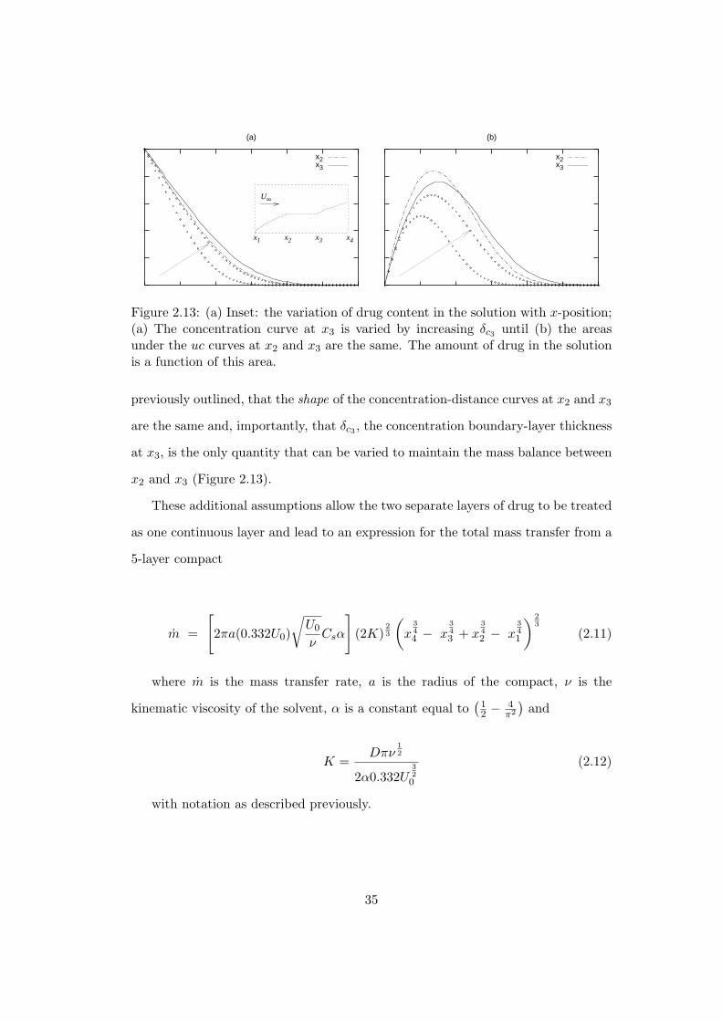
(a)

x2x3

(b)

x2x3

U∞

x1 x2 x3 x4

Figure 2.13: (a) Inset: the variation of drug content in the solution with x-position;(a) The concentration curve at x3 is varied by increasing δc3 until (b) the areasunder the uc curves at x2 and x3 are the same. The amount of drug in the solutionis a function of this area.

previously outlined, that the shape of the concentration-distance curves at x2 and x3

are the same and, importantly, that δc3 , the concentration boundary-layer thickness

at x3, is the only quantity that can be varied to maintain the mass balance between

x2 and x3 (Figure 2.13).

These additional assumptions allow the two separate layers of drug to be treated

as one continuous layer and lead to an expression for the total mass transfer from a

5-layer compact

m =

[

2πa(0.332U0)

√

U0

νCsα

]

(2K)23

(

x34

4 − x34

3 + x34

2 − x34

1

) 23

(2.11)

where m is the mass transfer rate, a is the radius of the compact, ν is the

kinematic viscosity of the solvent, α is a constant equal to(

12− 4

π2

)

and

K =Dπν

12

2α0.332U32

0

(2.12)

with notation as described previously.

35

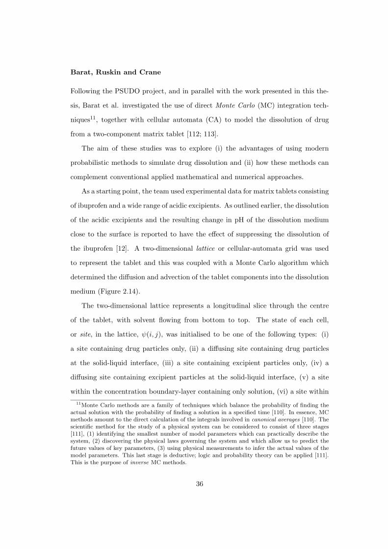
Barat, Ruskin and Crane

Following the PSUDO project, and in parallel with the work presented in this the-

sis, Barat et al. investigated the use of direct Monte Carlo (MC) integration tech-

niques11, together with cellular automata (CA) to model the dissolution of drug

from a two-component matrix tablet [112; 113].

The aim of these studies was to explore (i) the advantages of using modern

probabilistic methods to simulate drug dissolution and (ii) how these methods can

complement conventional applied mathematical and numerical approaches.

As a starting point, the team used experimental data for matrix tablets consisting

of ibuprofen and a wide range of acidic excipients. As outlined earlier, the dissolution

of the acidic excipients and the resulting change in pH of the dissolution medium

close to the surface is reported to have the effect of suppressing the dissolution of

the ibuprofen [12]. A two-dimensional lattice or cellular-automata grid was used

to represent the tablet and this was coupled with a Monte Carlo algorithm which

determined the diffusion and advection of the tablet components into the dissolution

medium (Figure 2.14).

The two-dimensional lattice represents a longitudinal slice through the centre

of the tablet, with solvent flowing from bottom to top. The state of each cell,

or site, in the lattice, ψ(i, j), was initialised to be one of the following types: (i)

a site containing drug particles only, (ii) a diffusing site containing drug particles

at the solid-liquid interface, (iii) a site containing excipient particles only, (iv) a

diffusing site containing excipient particles at the solid-liquid interface, (v) a site

within the concentration boundary-layer containing only solution, (vi) a site within

11Monte Carlo methods are a family of techniques which balance the probability of finding theactual solution with the probability of finding a solution in a specified time [110]. In essence, MCmethods amount to the direct calculation of the integrals involved in canonical averages [110]. Thescientific method for the study of a physical system can be considered to consist of three stages[111], (1) identifying the smallest number of model parameters which can practically describe thesystem, (2) discovering the physical laws governing the system and which allow us to predict thefuture values of key parameters, (3) using physical measurements to infer the actual values of themodel parameters. This last stage is deductive; logic and probability theory can be applied [111].This is the purpose of inverse MC methods.

36

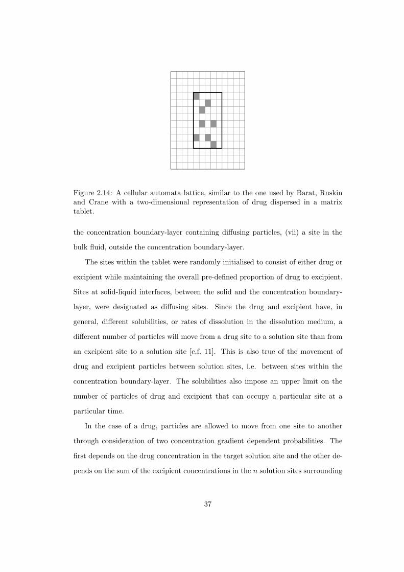
Figure 2.14: A cellular automata lattice, similar to the one used by Barat, Ruskinand Crane with a two-dimensional representation of drug dispersed in a matrixtablet.

the concentration boundary-layer containing diffusing particles, (vii) a site in the

bulk fluid, outside the concentration boundary-layer.

The sites within the tablet were randomly initialised to consist of either drug or

excipient while maintaining the overall pre-defined proportion of drug to excipient.

Sites at solid-liquid interfaces, between the solid and the concentration boundary-

layer, were designated as diffusing sites. Since the drug and excipient have, in

general, different solubilities, or rates of dissolution in the dissolution medium, a

different number of particles will move from a drug site to a solution site than from

an excipient site to a solution site [c.f. 11]. This is also true of the movement of

drug and excipient particles between solution sites, i.e. between sites within the

concentration boundary-layer. The solubilities also impose an upper limit on the

number of particles of drug and excipient that can occupy a particular site at a

particular time.

In the case of a drug, particles are allowed to move from one site to another

through consideration of two concentration gradient dependent probabilities. The

first depends on the drug concentration in the target solution site and the other de-

pends on the sum of the excipient concentrations in the n solution sites surrounding

37

the starting site.

Diffusion was modelled by using these probabilities to calculate the number of

drug particles that will move to each of the adjacent solution sites. The number of

excipient particles moving from one site to another is defined in terms of a variable

that takes a value between 1 and M , where M represents the number of drug

particles already present in the solution site.

The probability that particles will move, together with the maximum number of

particles that the adjacent site can accommodate, were used to give the number of

particles that actually move. The number of particles at each site is then summed to

arrive at new concentration levels after each time-step. The total number of particles

is not constant, as any particles that exit from the concentration boundary-layer into

the bulk fluid are discarded, advected out of the computational domain.

This advection process is implemented using the Pohlhausen concentration boundary-

layer profile described by Crane et al. [21]. All sites within the defined concentration

boundary-layer, i.e. between the surface, y = 0, and y = δc12, have a maximum

concentration which is defined by the Pohlhausen curve. If any cells have more than

this number of particles, the excess particles are advected away.

Between time-steps, the state of each site is also updated according to set rules,

e.g. if a site consisting only of drug is adjacent to a boundary-layer site at t = 0, then

this becomes a site within the concentration boundary-layer containing diffusing

particles at t = 1.

This model responds well to changes in drug and excipient solubilities, with

behaviour qualitatively similar to the results of experimentation [12; 113]. The

second paper by Barat et al. also presents investigations of the effect of drug loading

and initial porosity and cellular-automata behaviour on the simulation [113].

12δc is the concentration boundary-layer thickness.

38

2.3 Heat Transfer

2.3.1 Applying Heat Transfer Solutions to Mass Transfer Problems

Many textbooks and papers contain solutions to problems in heat transfer and specif-

ically the thermal boundary-layer equations [e.g. 94; 114; 102]. The mechanisms of

heat and mass transfer are mathematically equivalent and thermal solutions can be

applied with some minor modifications to problems in mass transfer [94].

As discussed by Crank [94], many technical workers experience difficulty in trans-

lating solutions of the heat transfer equations to mass transfer. Following Crank’s

discussion, we take the example of two simple geometrically similar 1-dimensional

heat and mass diffusion systems with constant properties, briefly discussing the cor-

respondence between the physical equations, parameters, variables and boundary

conditions.

After Kestin and Persen [108], the thermal boundary-layer or thermal energy

equation can be written as

u∂T

∂x+ v

∂T

∂y= αT

∂2T

∂y2(2.13)

for all cases of sub-sonic or low speed fluid flow. The equivalent mass transfer

equation is

u∂cA∂x

+ v∂cA∂y

= DAB∂2cA∂y2

(2.14)

where αT is the thermal diffusivity and DAB is the mass diffusivity, defined

previously. Diffusivities link fluxes with gradients. For low speed flows with constant

properties, the correspondence between the thermal and mass transfer equations

(Equations (2.13) and (2.14)) is clear.

As discussed by Crank [94], we identify the temperature T with concentration

c. The thermal diffusivity αT is identified with the mass diffusivity DAB.

39

2.3.2 Classical Work

Leveque

Leveque was the first to observe that when the transition from surface to freestream

temperature takes place across a very thin region close to the surface, the most

important fluid velocities, those inside this very thin region, change linearly with

normal distance from the surface, i.e. u = βy, where β is the normal velocity

gradient, the wall tangent, and x and y are the streamwise and normal directions

respectively (Figure 2.15)[107]. Schuh showed how to apply this idea to boundary-

layers, with the modification that the normal velocity gradient is a function of x,

u = β(x)y [115; 116]. Kestin and Persen [108] came to this idea independently,

outlining with clarity the solution that Schlichting describes in Boundary-Layer

Theory [117]. This solution, of the thermal boundary-layer equation for flows of large

Pr13, is Kestin and Persen’s, not Leveque’s. Kestin and Persen’s simplifications

work for large Pr or in any situation when the momentum boundary-layer thickness

is much greater than the thermal boundary-layer thickness. Perhaps surprisingly,

u = β(x)y results in a very good approximation, even for low Pr numbers, so that

only liquid metals with Pr much less than 1 cannot be treated this way [118].

In summary, Leveque proposed that u = βy. Schuh extended Leveque’s ob-

servation with u = β(x)y and a thermal boundary-layer solution for high Pr flow

with a wall temperature that varies as a fixed power of x. Kestin and Persen, like

Schuh, found an approximation of the form u = β(x)y and arrived at the thermal

boundary-layer solution presented by Schlichting [107].

Kestin and Persen

Kestin and Persen’s paper [108] describes solutions for heat transfer when the ther-

mal boundary-layer is contained entirely within the momentum boundary-layer, for

13Pr, the Prandtl number is the ratio of the momentum and mass diffusivities, i.e.ν

α.

40

Figure 2.15: Leveque’s linear velocity approximation. Quantities as defined in thetext.

various wall temperature distributions. For the problem of a flat plate with a tem-

perature jump at x = x0, they propose a substitution that reduces the parabolic

thermal boundary-layer equation (Equation (2.13)) to an ordinary differential equa-

tion. The solution to this equation, the temperature at any point in the fluid, can

be expressed as an incomplete gamma function. With the modifications outlined

above, this thermal solution can be adapted for application to the mathematically

equivalent problem of mass transfer from a flat plate. The resulting solution is

c = 1 −1

Γ(

13

)

∫ η3

0

e−tt−23dt (2.15)

where c is the concentration of solute at x and y, Γ(

1/3)

≈ 2.68 [119], t = η3

and η is given as

η =y√

τ0µ

[

9a∫ x

x0

√

τ0µdx

] 13

(2.16)

41

2.4 Numerical Methods

2.4.1 Finite Difference Methods

Introduction

As discussed by Dehghan [120], the main point of finite difference methods is to

obtain a solution to a PDE of a function by approximating the derivatives in the

equation using only values of the function at discrete points in space and time.

Taylor series expansions are most often used to obtain these approximations. It is

possible to classify Taylor series by their theoretical order of accuracy, allowing the

performance of different finite difference methods in terms of accuracy to be easily

compared. The modified equivalent partial differential equation method is a formal

methodology used for simple and direct comparison of finite difference schemes and

to identify and generate the most efficient schemes [121; 120; 122; 123].

There are three methods for approximating a continuous derivative using points

on a finite difference grid : forward or upwind differencing, backward or downwind

differencing and central differencing [121; 114]. When a PDE is discretised using

these methods, its derivatives at a point are calculated in terms of a combination

of the values of nearby nodes. For a given x, y position, forward differencing uses

function values at the previous x step on the grid, i − 1, to approximate deriva-

tives in y. Backward differencing uses function values at the next x step, i + 1,

to approximate derivatives in y. Central differencing at a grid position i, j uses

function values at the current i position to approximate derivatives in y. The use of

forward or backward differencing introduces a second order error termed numerical

dispersion or numerical diffusion which acts as an additional artificial diffusion or

viscosity term [121].

Artificial or numerical diffusion is an effect of solving continuous equations (in-

cluding the Navier-Stokes equations and the boundary-layer equations) discretely

on a fixed grid. Numerical diffusion is a smoothing of gradients that affects ad-

42

vected fluid properties, including momentum and other scalar quantities [124]. It

results from the spatial averaging that occurs between grid points. More specifically,

the approximation of the differential equations with discrete equations introduces a

truncation error14 which includes numerical diffusion as a component [125]. In gen-

eral, the discrete equations are more diffusive than the original differential equations

and so the discrete solution differs from the continuous solution. Numerical codes

are usually chosen so as to avoid numerical diffusion (especially when modelling

shock waves and similar phenomena which involve steep gradients), but in some

cases numerical diffusion helps to reduce problematic effects, such as singularities;

when viscous (physical) diffusion is not enough to ensure a stable solution, numeri-

cal diffusion can be used as a stabilising measure [126]. The effective viscosity is a

combination of both viscous and numerical diffusion [126]. The quantification of the

effects of numerical diffusion, especially when physical viscosity plays a major role

is important, such as in boundary-layer flows and mixing problems [126]. Numeri-

cal diffusion was quantified as a second-order error term (by Lantz and Chaudhari,

both in 1971) through the examination of a simple Taylor series expansion of the

original fluid property around a point, e.g. concentration, c(y). The modified par-

tial differential equation method, developed by Warming and Hyett, is a popular

method used to investigate the stability and accuracy of linear partial differential

equations [127]. A truncated version of the modified equation can be used to gain

insight into the nature of both dissipative and dispersive errors, a method used by

Dehghan in his review of various finite difference codes [120]. Dehghan’s modified

version of the one-dimensional advection-diffusion equation,∂c

∂t+ u

∂c

∂x− µ

∂2c

∂x2, is

∂c

∂t+ u

∂c

∂x− µ

∂2c

∂x2=u∆x

2(ω − λ)

∂2c

∂x2−u∆x2

6(2λ2 − 3ωλ+ 1 − 6k)

∂3c

∂x3+O[∆x3],

where w is a weight which controls the upwind bias, λ is the Courant number,

λ = u∆t/∆x, and k is the dimensionless diffusion number, k = µ∆t/∆x2. The

right hand side of this equation represents the truncation error. The first term, the

14See Section 2.4.1.

43

lowest order term, contains the numerical diffusion component. As detailed by De-

hghan, the modified version of the Crank-Nicolson scheme used in this thesis does

not contain numerical diffusion [120].

Finite difference methods are straightforward and well suited to problems involv-

ing regularly shaped regions or regions that can be transformed into regular regions

[121].

Explicit and Implicit Schemes

Finite-difference schemes can be explicit or implicit [114; 121] (Figure 2.4.1). An

explicit scheme is one where the downstream variables, u(x+ ∆x, y), v(x+ ∆x, y),

depend only on upstream values u(x, y), v(x, y). An implicit method, on the other

hand, is one where u(x + ∆x, y) and v(x + ∆x, y) depend also on u and v values

at the same x-step and where u(x+ ∆x, y) and v(x+ ∆x, y) must be solved simul-

taneously with all u,v values at x+ ∆x. Although explicit schemes are susceptible

to instability and errors can propagate rapidly if ∆x is too big (see Figure 2.4.1),

they are attractive for their simplicity. Maintaining solution stability by keeping ∆x

small, however, can lead to excessive computation. Implicit schemes, although more

computationally intensive per step, are generally unconditionally stable and allow

large ∆x, subject only to truncation errors [114]. In addition to having generally

better accuracy, implicit methods can be more efficient overall [121]. Understanding

when an implicit scheme ought to be used instead of an explicit scheme is therefore

an important study.

There are many examples of both explicit and implicit finite difference schemes,

all fit for different purposes and many texts and papers have been written on the

subject [e.g. 128; 121; 120]).

44

(a) (b)

Figure 2.16: In explicit schemes (a) small errors can rapidly propagate, renderingthe solution useless. Implicit schemes (b) on the other hand, damp out errors,preventing them from saturating the calculation. This diagram is for illustrationonly.

Finite Difference Schemes

Dehghan’s recent collection of papers on the subject of finite difference methods

[e.g. 120; 122; 123; 129] provides a comprehensive overview of the strengths and

weaknesses of different explicit and implicit finite difference schemes when used to

solve variations of the advection-diffusion equation (see Table 2.1 and Figure 2.18).

Overviews of the advantages and disadvantages of various finite difference schemes

are also given by [130; 131; 128; 121; 94; 114; 102]. These methods include the

Forward Time Centred Space (FTCS) explicit method, the upwind explicit method,

the Lax-Wendroff explicit method, the Crank-Nicolson semi-implicit method, the

Backward Time Centred Space (BTCS) implicit method, the upwind or backwards

implicit method, the Siemieniuch Gladwell implicit method, the Richtmyer modifi-

cation or backward differentiation implicit method, the Dufort-Frankel (or FQEFD,

Fast Quasi-Explicit Finite Difference) explicit method [121], the Hopscotch explicit

method, the Alternating Direction Implicit (ADI) method and the Strongly Implicit

Procedure (SIP) among others. Several common schemes are outlined in Figure 2.17.

Finite difference schemes are relatively simple, yet effective and widely used to solve

diffusion problems [e.g. 132].

45

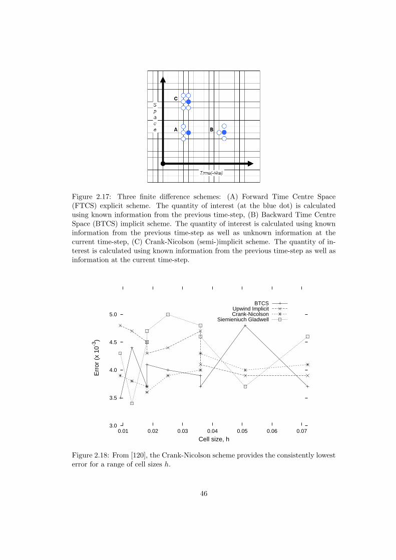
Figure 2.17: Three finite difference schemes: (A) Forward Time Centre Space(FTCS) explicit scheme. The quantity of interest (at the blue dot) is calculatedusing known information from the previous time-step, (B) Backward Time CentreSpace (BTCS) implicit scheme. The quantity of interest is calculated using knowninformation from the previous time-step as well as unknown information at thecurrent time-step, (C) Crank-Nicolson (semi-)implicit scheme. The quantity of in-terest is calculated using known information from the previous time-step as well asinformation at the current time-step.

3.0

3.5

4.0

4.5

5.0

0.01 0.02 0.03 0.04 0.05 0.06 0.07

Err

or (

x 10

-3)

Cell size, h

BTCSUpwind ImplicitCrank-Nicolson

Siemieniuch Gladwell

Figure 2.18: From [120], the Crank-Nicolson scheme provides the consistently lowesterror for a range of cell sizes h.

46

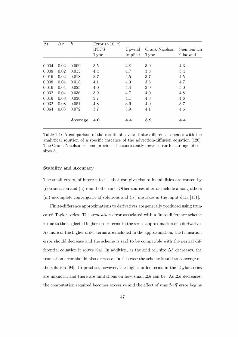
∆t ∆x h Error (×10−3)BTCS Upwind Crank-Nicolson SiemieniuchType Implicit Type Gladwell

0.004 0.02 0.009 3.5 4.8 3.9 4.30.008 0.02 0.013 4.4 4.7 3.8 3.40.016 0.02 0.018 3.7 4.5 3.7 4.50.008 0.04 0.018 4.1 4.3 3.6 4.70.016 0.04 0.025 4.0 4.4 3.9 5.00.032 0.04 0.036 3.9 4.7 4.0 4.80.016 0.08 0.036 3.7 4.1 4.3 4.60.032 0.08 0.051 4.8 3.9 4.0 3.70.064 0.08 0.072 3.7 3.9 4.1 4.6

Average 4.0 4.4 3.9 4.4

Table 2.1: A comparison of the results of several finite-difference schemes with theanalytical solution of a specific instance of the advection-diffusion equation [120].The Crank-Nicolson scheme provides the consistently lowest error for a range of cellsizes h.

Stability and Accuracy

The small errors, of interest to us, that can give rise to instabilities are caused by

(i) truncation and (ii) round-off errors. Other sources of error include among others

(iii) incomplete convergence of solutions and (iv) mistakes in the input data [131].

Finite-difference approximations to derivatives are generally produced using trun-

cated Taylor series. The truncation error associated with a finite-difference scheme

is due to the neglected higher-order terms in the series approximation of a derivative.

As more of the higher order terms are included in the approximation, the truncation

error should decrease and the scheme is said to be compatible with the partial dif-

ferential equation it solves [94]. In addition, as the grid cell size ∆h decreases, the

truncation error should also decrease. In this case the scheme is said to converge on

the solution [94]. In practice, however, the higher order terms in the Taylor series

are unknown and there are limitations on how small ∆h can be. As ∆h decreases,

the computation required becomes excessive and the effect of round-off error begins

47

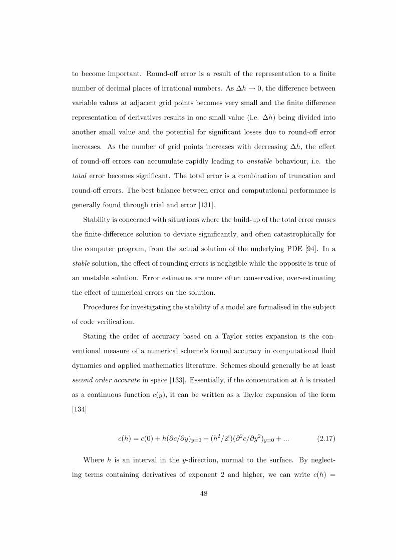
to become important. Round-off error is a result of the representation to a finite

number of decimal places of irrational numbers. As ∆h→ 0, the difference between

variable values at adjacent grid points becomes very small and the finite difference

representation of derivatives results in one small value (i.e. ∆h) being divided into

another small value and the potential for significant losses due to round-off error

increases. As the number of grid points increases with decreasing ∆h, the effect

of round-off errors can accumulate rapidly leading to unstable behaviour, i.e. the

total error becomes significant. The total error is a combination of truncation and

round-off errors. The best balance between error and computational performance is

generally found through trial and error [131].

Stability is concerned with situations where the build-up of the total error causes

the finite-difference solution to deviate significantly, and often catastrophically for

the computer program, from the actual solution of the underlying PDE [94]. In a

stable solution, the effect of rounding errors is negligible while the opposite is true of

an unstable solution. Error estimates are more often conservative, over-estimating

the effect of numerical errors on the solution.

Procedures for investigating the stability of a model are formalised in the subject

of code verification.

Stating the order of accuracy based on a Taylor series expansion is the con-

ventional measure of a numerical scheme’s formal accuracy in computational fluid

dynamics and applied mathematics literature. Schemes should generally be at least

second order accurate in space [133]. Essentially, if the concentration at h is treated

as a continuous function c(y), it can be written as a Taylor expansion of the form

[134]

c(h) = c(0) + h(∂c/∂y)y=0 + (h2/2!)(∂2c/∂y2)y=0 + ... (2.17)

Where h is an interval in the y-direction, normal to the surface. By neglect-

ing terms containing derivatives of exponent 2 and higher, we can write c(h) =

48

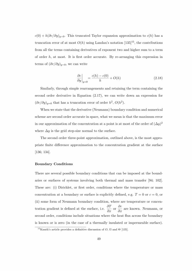
c(0) + h(∂c/∂y)y=0. This truncated Taylor expansion approximation to c(h) has a

truncation error of at most O(h) using Landau’s notation [135]15, the contributions

from all the terms containing derivatives of exponent two and higher sum to a term

of order h, at most. It is first order accurate. By re-arranging this expression in

terms of (∂c/∂y)y=0, we can write

∂c

∂y

∣

∣

∣

∣

y=0

=c(h) − c(0)

h+O(h) (2.18)

Similarly, through simple rearrangements and retaining the term containing the

second order derivative in Equation (2.17), we can write down an expression for

(∂c/∂y)y=0 that has a truncation error of order h2, O(h2).

When we state that the derivative (Neumann) boundary condition and numerical

scheme are second order accurate in space, what we mean is that the maximum error

in our approximation of the concentration at a point is at most of the order of (∆y)2

where ∆y is the grid step-size normal to the surface.

The second order three-point approximation, outlined above, is the most appro-

priate finite difference approximation to the concentration gradient at the surface

[136; 134].

Boundary Conditions

There are several possible boundary conditions that can be imposed at the bound-

aries or surfaces of systems involving both thermal and mass transfer [94; 102].

These are: (i) Dirichlet, or first order, conditions where the temperature or mass

concentration at a boundary or surface is explicitly defined, e.g. T = 0 or c = 0, or

(ii) some form of Neumann boundary condition, where are temperature or concen-

tration gradient is defined at the surface, i.e.∂T

∂xor

∂c

∂xare known. Neumann, or

second order, conditions include situations where the heat flux across the boundary

is known or is zero (in the case of a thermally insulated or impermeable surface).

15Knuth’s article provides a definitive discussion of O, Ω and Θ [135].

49

When the heat or mass flux is known, it may take the form of a radiation bound-

ary condition. This is when the flux is proportional to the difference between the

temperatures at the surface and in the medium far from the surface. A convective

boundary condition is similar to a radiation boundary condition except that the flux

at the surface is not only related to the difference in temperatures or concentrations

between the surface and far-field, but also on the flow velocity of the fluid. Other

types of Neumann condition are described in textbooks [e.g. 94; 114; 102].

The derivative boundary conditions are implemented as forward-difference sec-

ond order, 3-point approximations, namely [136]

∂c

∂y=

−c2 + 4c1 − 3c02∆y

= 0 (2.19)

⇒ c0 =4c1 − c2

3(2.20)

where c0 is the unknown concentration value at the surface at grid position

i, while c1 and c2 are the concentration values at ∆y and 2∆y from the surface

respectively, also calculated at i. The error associated with this boundary condition,

based on a Taylor series expansion, is of the order of at most (∆y)2 [134].

Solution of Linear Systems of Equations

The Tridiagonal Matrix Algorithm (TDMA), or Thomas Algorithm, is a compu-

tationally efficient technique for solving tridiagonal linear simultaneous equations

[121]. According to [137], it was first proposed by [138] and subsequently applied to

systems of parabolic equations by [139]. The technique described [137] is a simpli-

fied version of the Gaussian elimination method that works for tridiagonal matrices

(see also [140], [141], [114], and [131]).

50

2.4.2 Verification and Validation

Uncertainty is the estimated percentage by which an observation or calculation dif-

fers from reality [142]. Uncertainty can be classified into three broad sub-categories:

(1) uncertainty in the input data, boundary conditions and so forth; (2) uncertainty

in the model used and (3) uncertainty arising from numerical error. Uncertainty

ultimately results from a lack of information [143]16. Numerical simulation hinges

on the assumption that as the grid size h → 0, the numerical solution converges to

the continuum differential equation and the exact solution [142]. The objective of

verification and validation is to demonstrate that this assumption is true for each

implementation. Verification is about solving the equations correctly and validation

is about solving the correct model equations with the correct methods [142]. Stated

simply, verification is about mathematics while validation is about physics [145].

Verification

Verification, taken as being synonymous with code verification, is concerned with

ensuring that the numerical methods chosen solve the chosen equations correctly, to

within an acceptable accuracy [146; 147; 145; 143; 68; 148]. Celik’s [149] method-

ology for estimating and reporting the discretisation error of a numerical scheme17

is important and worth reviewing. The key points are (i) that the computer code

must be referenced and previous verification studies relating to it must be described,

(ii) the theoretical or formal order of accuracy of the numerical scheme in each di-

16The Journal of Fluids Engineering acknowledges that there is no standard method for evaluatingthe uncertainty in numerical simulation [144]. It does, however, outline criteria to be consideredfor publication in the journal. These include: (1) precise description of the numerical methodincluding a formal assessment of the truncation error introduced by individual terms in the governingequations; (2) the numerical method must be at least formally second-order accurate in space (basedon a Taylor series expansion) for nodes in the interior of the grid; (3) solutions over a range ofsignificantly different grid resolutions should be presented to demonstrate grid independence or grid-convergent results; (4) boundary and initial condition implementations must be clearly described;(5) while the numerical method must be carefully described, all pertinent references must be citedwithin the paper to allow proper evaluation of the code; (6) comparison to appropriate analyticalbenchmark solutions may be used to demonstrate accuracy under certain conditions; (7) comparisonwith reliable experimental results is appropriate, provided experimental uncertainty is established.

17Adopted as a requirement for submitted work by the J. Fluid. Eng. [144].

51

mension for each equation solved must be stated, (iii) for iterative schemes, there

should be at least a three orders of magnitude decrease in the normalised residuals

for each equation solved, (iv) for time dependent schemes, the convergence of the

solution at each time-step should be checked and (v) a variation of the Richardson

Extrapolation (RE) method [150; 151], known as the Grid Convergence Index (GCI)

method [149; 152], is recommended for assessing the discretisation error. Systematic

grid refinements using variations of the RE method are the most common way of

estimating the actual discretisation error associated with a simulation [142]. An

implementation of the GCI method is outlined in the next chapter.

Validation

Validation is the comparison of computational results with experiment [142; 153].

The difficulty with validation, however, is determining (i) how exactly to validate

and (ii) what we can say about the correspondence of our model’s predictions with

reality once a validation procedure has been completed. Oberkampf and Trucano

tackle the second point by observing that validation says nothing about prediction,

only about the correspondence of model results for known situations [153]. Valida-

tion equips us to infer how the model will perform in situations for which it has

not been validated [153]. The first point can be captured by asking three ques-

tions: (1) how can a validation be expressed quantitatively? (2) Can we develop a

useful methodology for determining what validation is required? (3) What are the

important features of a validation experiment? The authors proceed to define six

guidelines for carrying out validations of simulations. These are, essentially, that

validation experiments should: (i) be defined by a team comprising experimental-

ists, modellers, coders, and users; (ii) capture the essential physics of the system

under investigation; (iii) attempt to emphasise the complementarity of simulation

and physical experiment; (iv) maintain independence between data acquisition from

simulation and physical experiment; (v) proceed from simple to complex and from

52

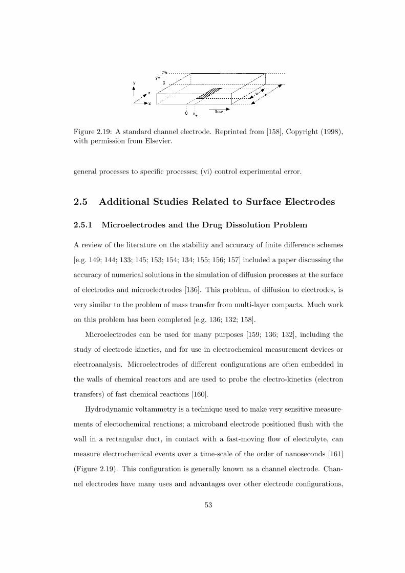
Figure 2.19: A standard channel electrode. Reprinted from [158], Copyright (1998),with permission from Elsevier.

general processes to specific processes; (vi) control experimental error.

2.5 Additional Studies Related to Surface Electrodes

2.5.1 Microelectrodes and the Drug Dissolution Problem

A review of the literature on the stability and accuracy of finite difference schemes

[e.g. 149; 144; 133; 145; 153; 154; 134; 155; 156; 157] included a paper discussing the

accuracy of numerical solutions in the simulation of diffusion processes at the surface

of electrodes and microelectrodes [136]. This problem, of diffusion to electrodes, is

very similar to the problem of mass transfer from multi-layer compacts. Much work

on this problem has been completed [e.g. 136; 132; 158].

Microelectrodes can be used for many purposes [159; 136; 132], including the

study of electrode kinetics, and for use in electrochemical measurement devices or

electroanalysis. Microelectrodes of different configurations are often embedded in

the walls of chemical reactors and are used to probe the electro-kinetics (electron

transfers) of fast chemical reactions [160].

Hydrodynamic voltammetry is a technique used to make very sensitive measure-

ments of electochemical reactions; a microband electrode positioned flush with the

wall in a rectangular duct, in contact with a fast-moving flow of electrolyte, can

measure electrochemical events over a time-scale of the order of nanoseconds [161]

(Figure 2.19). This configuration is generally known as a channel electrode. Chan-

nel electrodes have many uses and advantages over other electrode configurations,

53

Figure 2.20: Two microband electrodes positioned in a channel flow. Reprintedfrom [132], Copyright (2005), with permission from Elsevier.

including increased sensitivity and range of measurement [141; 158].

A recent paper describes a problem very similar to that of drug dissolution from

multi-layer compacts, the diffusion to two microband electrodes in a channel flow

(Figure 2.20) [132]. Studies have shown that this double-electrode configuration

allows experimental access to additional mechanistic information about the electro-

chemical processes [141]. Instead of electrodes and insulators, however, we have

diffusing regions of drug and impermeable surfaces. The mathematical descriptions

almost coincide.

As with our problem, the diffusion process is described by a simplified version

of the time-dependent advection-diffusion equation, which is written as

∂c

∂t+ u

∂c

∂x+ v

∂c

∂y= D

∂2c

∂y2(2.21)

where c is the concentration of the electroactive species, x and y are the stream-

wise and normal directions, as usual, and u and v are their corresponding velocity

components. D [m2s−1] is the diffusion coefficient of the process. In addition, it

is assumed that mass transfer is dominated by convection in the axial, x, direction

and diffusion in the normal, y-direction [162]. In a recent paper [132], the Leveque

approximation to the velocity profile close to the electrode surfaces is given as

u(y) = u0

(

1 −(h− y)2

h2

)

(2.22)

where u0 is the velocity at the centre of the channel, y the distance normal to

54

the surface, and h is the half-height of the channel. An implicit finite difference

solution to Equation (2.21) is implemented [163; 164; 165].

2.5.2 Singularities in the Numerical Solutions

A significant portion of the microelectrode literature is given to the consideration

of singularities in the numerical solutions. Standard numerical methods (such as

finite difference schemes) can have poor accuracy when used to model the mass

transfer to electrodes, especially close to the edge of the electrode, where it meets

the surrounding insulator [136]. This is mainly due to the presence of a boundary

singularity at the interface between the two surfaces. The singularity normally

takes the form of a discontinuity in the first derivative of the concentration values

at the point where the electrode meets the insulator [136]; two conflicting boundary

conditions are imposed on the same point, a Dirichlet condition on the electrode

surface and a Neumann (derivative) condition at the insulator surface [159]. Lines

of constant concentration are parallel to the surface close to the electrode surface,

where the Dirichlet condition is imposed, and perpendicular to the surface of the

insulator where the zero-flux Neumann condition pertains. At the interface between

the electrode and the insulator, these conditions cause a discontinuity in the normal

derivative of concentration and lead to a singular solution to the local current density

at the edge of the electrode.

This can be stated as follows - for a disk-shaped electrode in a steady state,

where r and z represent the radial and axial spatial coordinates respectively and c

is the normalised concentration in the electrolyte, mass transport to the electrode

can be described by the steady-state two-dimensional cylindrical diffusion equation

[166; 136; 167]:

∂2c

∂r2+

1

r

∂c

∂r+∂2c

∂z2= 0 (2.23)

with the following boundary conditions

55

(1) z = 0 r > a∂c

∂z= 0

(2) z = 0 r ≤ a u = 0

(3) z = 0 r = 0∂c

∂r= 0

(4) z → ∞ r ≥ 0 c = 1

(5) z = 0 r → ∞ c = 1

where a is the radius of the circular insulator. A singularity then arises at r = a,

z = 0, where boundary conditions (1) and (2) are inconsistent.

Although, as Gavaghan [168; 136] notes, this is a well known problem [169; 170;

171; 94], there is no consensus in the literature about the seriousness of the effect of

this boundary singularity on the accuracy of solutions to related problems. Fox and

Sankar [171] state that for some elliptic problems, the presence of a discontinuity

may not be serious since the solution remains well behaved in the solution region and

most of the error is confined to the neighbourhood of the singularity. At sufficient

distances from the singularity, the numerical results are still accurate. For the

diffusion equation, difference solutions quickly approach the analytical solution after

a few time-steps [94]. This is true of the steady-state advection-diffusion equation

with the streamwise step instead of time-steps. Surveying recent mathematical

investigations of the mass transfer to electrodes, [134; 172; 173; 141; 174; 164;

165; 155; 160; 161; 175; 176; 132], the authors make no mention of the boundary

singularity as being important to the accuracy of their solutions. Gavaghan [136],

however, argues that an accurate solution to this problem is only possible if special

techniques are used to handle the singularity; [168], [166], [128], [136], [177], [159],

[178], [179] [167] consider the effect of the boundary singularity on the current flux

values.

In his PhD thesis, Alden reviews the problem of boundary singularities in elec-

trochemistry and lists the two main examples: the spatial discontinuity that occurs

at the boundary between an electrode and an insulator, and the temporal disconti-

nuity that occurs when the electrode potential is stepped [121]. In both situations,

56

the current flux tends to infinity at a point. Alden [121] describes three methods for

dealing with boundary singularities (as outlined by [168; 180; 136; 178; 179]). These

are to: (1) increase the mesh density close to the singularity or across the whole com-

putational region, limiting the extent to which the errors can spread (for example

[159; 181]), (2) subtract the effects of the singularity by compensating for it [180],

(3) use a conformal mapping to transform the computational region, eliminating the

singularity altogether (for example [173]).

Modelling diffusion to and from these microband electrodes has many similar-

ities to the work presented in the first study of this thesis, i.e. there are similar

system configurations and governing equations. Indeed, the original drug delivery

problem tackled by Kenny [99] owed much to earlier work on mass transfer to and

from microband electrodes [101]. The mathematical and numerical challenges facing

workers in this area are similar to the challenges facing those modelling mass transfer

in pharmaceutical devices and the volume of work already completed in modelling

electrodes serves to underscore how much there is to be done in modelling drug

dissolution.

2.6 Software

2.6.1 Commercial Code

Fluent

The Fluent solver is a C-based computer program for modelling fluid flow and

heat transfer involving three-dimensional complex geometries [106]. It uses a finite

volume method to solve the Navier-Stokes equations and includes several turbulence

models. The finite volume method is commonly used to solve partial differential

equations by calculating the value of a conserved variable averaged across a volume.

The solver allows the user to set a range of parameters, including specification of the

boundary conditions, the material properties and the type of flow model. Gambit is

57

a pre-processor for CFD analysis, bundled with the Fluent solver [106]. Gambit is

used to build model geometries and generate meshes. It can also import, modify and

mesh geometries created by third-party computer aided design or computer aided

engineering packages. Boundary conditions are then specified and the resulting mesh

file exported to the solver.

2.6.2 Open Code

Python

Python is a general purpose, object-oriented, open-source, interpreted programming

language. Since the 1990s, Python has grown in popularity and is now used by

hundreds of thousands of programmers in fields as diverse as bioinformatics and

computer-generated imagery [182; 183; 184]. Python was designed to appeal to

Unix/C programmers and to be reusable and readable with minimal coding time

[185]. It tends to be used mainly by engineers and scientists.

Python is a scripting language. Advantages of scripting include typeless datatypes

to simplify interaction between components and to accelerate application build times

[186]. Python has operating system interfaces, a large standard library, and is exten-

sible in C and C++. Other advantages of Python include its wide range of features

(datatypes, modules), stability, syntax, small core and modules, widely available

documentation, and the available support. It is also free [187; 183]. Python has a

large number of libraries including NumPy, its extensive numerical library. Applica-

tion development is generally faster with Python than with C or Fortran and takes

less code to express an algorithm. It is modular and easily extendible. It can be used

interactively like MATLAB. Python can also be used to glue existing C/C++ etc.

modules together. Python’s popularity means that tools exist for many applications

where C and Fortran dominate, e.g. a Python binding exists for the CGNS 18 (the

other CGNS bindings are for C, C++ and Fortran77/Fortran90)[188].

18Computational Fluid Dynamics General Notation System.

58

Python is available for almost every platform including Windows, Linux/Unix,

Mac OS X, OS/2, Amiga, Palm OS, WinCE, Java and .NET. It may also run on

other system configurations once there is a C compiler available.

Gnuplot

One visualisation tool used to produce many of the graphs in this thesis is Gnuplot.

Originally developed in 1986, Gnuplot is a free, command-driven interactive plotting

program; it is a powerful tool for plotting mathematical functions and numerical data

[189; 190]. Gnuplot is extremely robust and can produce graphs in several formats,

including even plaintext [191]. In addition to its interactive functions, Gnuplot can

be used in batch mode with text scripts saved as plot (.plt) files. Batch mode is

particularly useful when producing many similar graphs from a series of experiments

[192]. Gnuplot is available for most operating systems.

2.7 Chapter Summary and Conclusions

This chapter began with a review of the drug industry and explained with examples

why simulation is important for pharmaceutics. The ideas in this thesis draw most

heavily on the results of the PSUDO project. This project and other important con-

tributions to the development of mathematical simulation of multi-layered systems

were reviewed. Some of the key ideas discovered in the course of researching this

work were discussed and placed in context. Finite-difference schemes and related

numerical methods, together with the importance of verification and validation,

were introduced. The work reviewed in this chapter forms the basis for much of

the further development presented in this thesis and leads on to the related studies

which are described in Chapters 4 and 5.

59

Chapter 3

Theory and Methods, Study 1

This chapter introduces the theory and methods associated with the core inves-

tigation of the initial drug dissolution rate from a cylindrical tablet in the USP

apparatus. The aim of this work was to make progress in understanding drug disso-

lution in the USP apparatus; to investigate different problems inspired by aspects of

tablet dissolution in the USP apparatus and to build several components of a com-

plete model. The individual investigations each contribute to the argument that

simulation is useful for pharmaceutics. Central to this thesis was an investigation

of the tablet’s initial dissolution rate. This involved the development of a robust

finite-difference solution and a study of the differences between existing solutions

and a new numerical solution. This first study was followed by a second in which

the flow about a cylinder in cross-flow was considered, with a specific investigation

of the flow around a meteorological mast. This has utility for the wind energy in-

dustry. The third and final part of the thesis was a study of particle dissolution in

the USP apparatus. Theory and methods related to the first investigation follow.

60

3.1 Motivations for Modelling Multi-Layered Tablets

As with previous work, the multi-layer configuration was chosen as the topic for

this study for reasons including: (i) it is a simple starting point, with well-defined

regions of drug and excipient [21], (ii) techniques used to model this system may be

applied to uniformly mixed multi-component compacts [20].

3.2 Model Set-Up

The drug component was taken to be benzoic acid with a diffusion coefficient of

1.236 × 10−5 cm2 s−1 and a solubility in the solvent (0.1M HCl at 37o) of 4.55 mg

cm−3 [104]. The viscosity of the fluid was assumed to be that of the solvent, 0.00786

cm2 s−1 . The axial freestream velocity past the compact was set as 1.83 cm s−1

[17]. The compacts were 0.85 cm in height and of radius a = 0.65 cm. Quantity

values are detailed in Tables 3.1, 3.2 and 3.3. Experiments, used to validate the

results presented in this thesis, were carried out for compacts consisting of [17]:

1. A single layer of benzoic acid (BA).

2. A 3-layer system of benzoic acid and salicylic acid (SA): BA/SA/BA.

3. A 5-layer system of benzoic acid and salicylic acid (SA): BA/SA/BA/SA/BA.

Quantity Symbol Value

Solubility Cs 4.55 mg cm−3

Diffusivity D 1.236 × 10−5 cm2 s−1

Schmidt Number Sc 637

Table 3.1: Important quantities for benzoic acid systems.

61


Solubility Cs 2.58 × 10−3 mg cm−3

Diffusivity D 1.13167 × 10−5 cm2 s−1

Schmidt Number Sc 695

Table 3.2: Important quantities for salicylic acid systems.


Advection Velocity U∞ 1.83 cm s−1

Kinematic Viscosity (HCl) ν 0.00786 cm2 s−1

Tablet Length L 0.85 cm

Tablet Radius a 0.65 cm

Table 3.3: Important quantities common to all systems considered. Kinematic vis-cosity is given for 0.1M HCl at 37C.

3.3 Governing Equations

The two-dimensional velocity and concentration boundary-layer equations for steady,

incompressible, viscous flow are central to this thesis and their solution forms the

basis of much of the work described. We show how the general form of the convec-

tion transfer, or boundary-layer, equations can be simplified for the problem under

consideration in this thesis.

3.3.1 Boundary-Layer Equations

The Navier-Stokes equations for two-dimensional incompressible flow with constant

material properties are [102]

ρ

(

u∂u

∂x+ v

∂u

∂y

)

= ρX −∂p

∂x+ µ∆u (3.1)

62

ρ

(

u∂v

∂x+ v

∂v

∂y

)

= ρY −∂p

∂y+ µ∆v (3.2)

where ρ is the density of the fluid, assumed constant, µ is the viscosity, u and

v are the velocity components in the streamwise (x) and normal (y) directions

respectively, X and Y are components of the resultant mass force vector K, p is the

fluid pressure, and ∆ =

(

∂2

∂x2+

∂2

∂y2

)

. The mass continuity equation is

∂u

∂x+∂v

∂y= 0 (3.3)

with the variables just defined. Simplified from the Navier-Stokes equations,

the advection-diffusion equation is used to model the drug mass transfer from the

surface of the compacts. In its general two-dimensional form, this is written

∂c

∂t+ u

∂c

∂x+ v

∂c

∂y=

∂

∂x

(

DAB∂c

∂x

)

+∂

∂y

(

DAB∂c

∂y

)

+ nA (3.4)

where c is the concentration of drug, DAB is its concentration-independent diffu-

sion coefficient and nA is the net rate increase of concentration as a result of chemical

reaction. Derivations of this equation, arrived at by physical considerations, can be

found in textbooks [e.g. 193; 102].

Simplifications

For the problem under consideration, we can make significant simplifications to the

convection transfer equations. We assume saturation concentration, Cs, at the solid-

liquid interface. This is achieved by ensuring that the concentration of drug in the

tablet is very much higher than the drug solubility in the liquid solvent; as long as

drug is available, this will maintain the concentration of drug as Cs at the dissolution

front and the release rate from the surface will be constant [32]. In addition, if the

Schmidt number (Sc, defined in a footnote in the last chapter) is large, the surface

curvature may be neglected and the problem reduces to steady two-dimensional

63

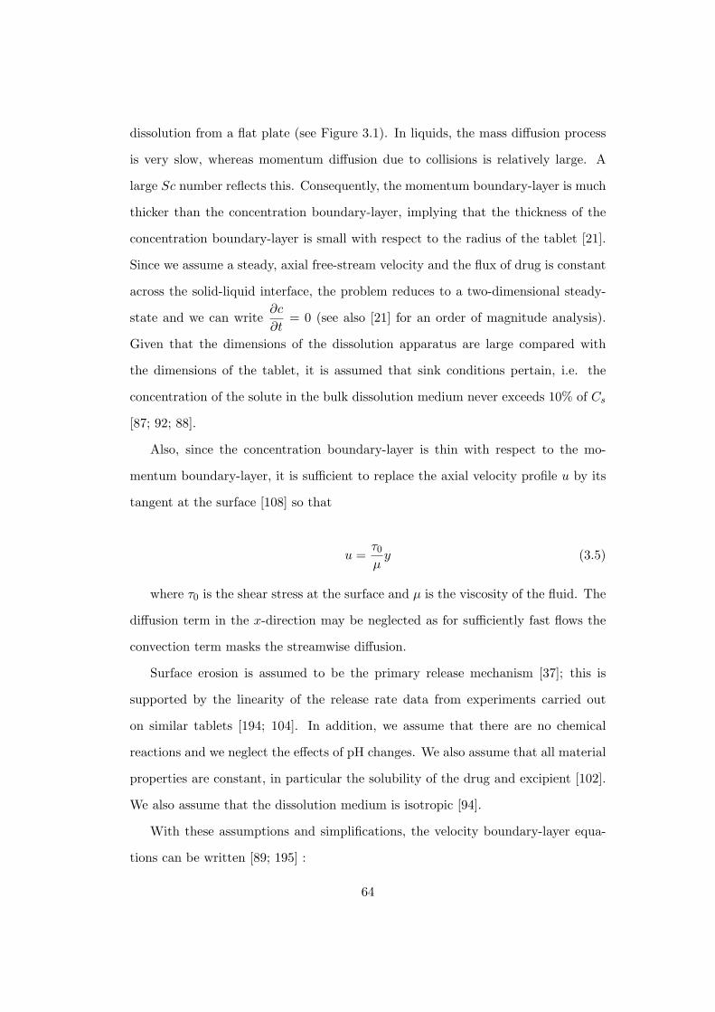
dissolution from a flat plate (see Figure 3.1). In liquids, the mass diffusion process

is very slow, whereas momentum diffusion due to collisions is relatively large. A

large Sc number reflects this. Consequently, the momentum boundary-layer is much

thicker than the concentration boundary-layer, implying that the thickness of the

concentration boundary-layer is small with respect to the radius of the tablet [21].

Since we assume a steady, axial free-stream velocity and the flux of drug is constant

across the solid-liquid interface, the problem reduces to a two-dimensional steady-

state and we can write∂c

∂t= 0 (see also [21] for an order of magnitude analysis).

Given that the dimensions of the dissolution apparatus are large compared with

the dimensions of the tablet, it is assumed that sink conditions pertain, i.e. the

concentration of the solute in the bulk dissolution medium never exceeds 10% of Cs

[87; 92; 88].

Also, since the concentration boundary-layer is thin with respect to the mo-

mentum boundary-layer, it is sufficient to replace the axial velocity profile u by its

tangent at the surface [108] so that

u =τ0µy (3.5)

where τ0 is the shear stress at the surface and µ is the viscosity of the fluid. The

diffusion term in the x-direction may be neglected as for sufficiently fast flows the

convection term masks the streamwise diffusion.

Surface erosion is assumed to be the primary release mechanism [37]; this is

supported by the linearity of the release rate data from experiments carried out

on similar tablets [194; 104]. In addition, we assume that there are no chemical

reactions and we neglect the effects of pH changes. We also assume that all material

properties are constant, in particular the solubility of the drug and excipient [102].

We also assume that the dissolution medium is isotropic [94].

With these assumptions and simplifications, the velocity boundary-layer equa-

tions can be written [89; 195] :

64

u∂u

∂x+ v

∂u

∂y= ν

∂2u

∂y2(3.6)

∂u

∂x+∂v

∂y= 0 (3.7)

While the concentration boundary-layer equation, Equation (3.4), can be written

in its simplified form as

u∂c

∂x+ v

∂c

∂y= D

∂2c

∂y2(3.8)

The boundary-layer equations are second order, linear, homogeneous and parabolic

as opposed to the Navier-Stokes equations which are elliptic [131; 130]. The sim-

plified thermal and concentration boundary-layer equations are characterised by

advection terms on the left-hand side and a diffusion term on the right-hand side.

These equations describe low-speed forced convection flows.

Non-Dimensional Form

We take the concentration boundary-layer equation. The dimensionless parameters

x′ and y′ are defined as

x′ =x

Land y′ =

y

L

Where L is some characteristic length of the system of interest. For a flat plate,

for example, this would usually be the length of the plate, while for a cylinder, the

characteristic length is normally taken as its diameter. The velocity components u

and v can be non-dimensionalised by defining

u′ =u

Uand v′ =

v

U

Where U is the free-stream fluid velocity. Finally, concentration can be non-

dimensionalised by writing

65

c′ =c− Cs

C∞ − Cs

Substituting these expressions into the simplified concentration boundary-layer

equation, Equation (3.8), yields the dimensionless concentration boundary-layer

equation, which we can write

u′∂c′

∂x′+ v′

∂c′

∂y′=

D

UL

∂2c′

∂y′2(3.9)

with the boundary conditions c′|y=0 = 0, c′|y=∞ = 0. The equation can also be

written in terms of the dimensionless Re and Sc numbers,

u′∂c′

∂x′+ v′

∂c′

∂y′=

1

ReLSc

∂2c′

∂y′2(3.10)

where ReL is the Reynolds number associated with the characteristic length L1.

Writing the boundary-layer equations and the associated boundary conditions in a

dimensionless form is the most efficient and useful presentation, allowing us to see

the important parameters in their correct context [114]. Dimensionless equations

allow us to apply the results for one particular system to another system that is

geometrically similar [102].

3.3.2 Boundary and Initial Conditions

We are concerned only with the drug mass transfer rate and assume no interaction

between the two components, so the boundary conditions are

1See the Glossary for a brief discussion of this important parameter.

66

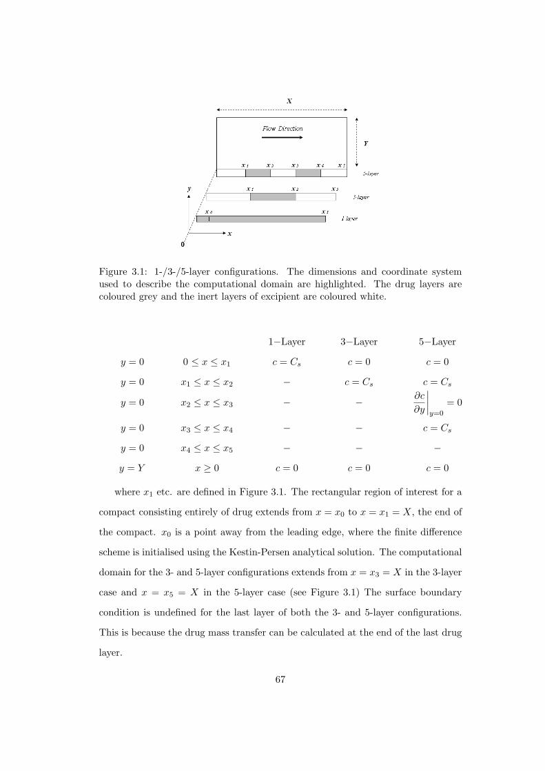
Figure 3.1: 1-/3-/5-layer configurations. The dimensions and coordinate systemused to describe the computational domain are highlighted. The drug layers arecoloured grey and the inert layers of excipient are coloured white.

1−Layer 3−Layer 5−Layer

y = 0 0 ≤ x ≤ x1 c = Cs c = 0 c = 0

y = 0 x1 ≤ x ≤ x2 − c = Cs c = Cs

y = 0 x2 ≤ x ≤ x3 − −∂c

∂y

∣

∣

∣

∣

y=0

= 0

y = 0 x3 ≤ x ≤ x4 − − c = Cs

y = 0 x4 ≤ x ≤ x5 − − −

y = Y x ≥ 0 c = 0 c = 0 c = 0

where x1 etc. are defined in Figure 3.1. The rectangular region of interest for a

compact consisting entirely of drug extends from x = x0 to x = x1 = X, the end of

the compact. x0 is a point away from the leading edge, where the finite difference

scheme is initialised using the Kestin-Persen analytical solution. The computational

domain for the 3- and 5-layer configurations extends from x = x3 = X in the 3-layer

case and x = x5 = X in the 5-layer case (see Figure 3.1) The surface boundary

condition is undefined for the last layer of both the 3- and 5-layer configurations.

This is because the drug mass transfer can be calculated at the end of the last drug

layer.

67

j

i

∆x

∆y

0 1 2 3 N0

1

2

3

M

Figure 3.2: Finite difference grid; flow from left to right, compact streamwise alongthe bottom. A 5-layer compact is illustrated with the diffusing drug layers high-lighted as bold black lines.

3.4 Numerical Methods

3.4.1 Introduction

To obtain a finite difference solution, the region of interest is covered by a grid with

solutions calculated at the intersection points [120]. For a two-dimensional grid, the

grid intersection points or nodes are denoted by two indices, i and j, corresponding

to the point’s x and y location [102]. The grid spacing in the x direction is ∆x and

∆y in the y direction [94]. The indices run from 1 to M in the x direction and 1 to

N in the y direction. We can write

• xi = i∆x, i = 0, 1, 2, ...,M

• yj = j∆y, j = 0, 1, 2, ..., N

parallel to the x and y coordinate axes [120]. The grid cell size is defined as

h =√

∆x∆y.

68

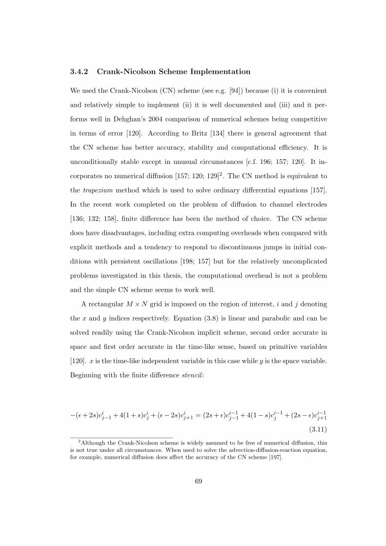
3.4.2 Crank-Nicolson Scheme Implementation

We used the Crank-Nicolson (CN) scheme (see e.g. [94]) because (i) it is convenient

and relatively simple to implement (ii) it is well documented and (iii) and it per-

forms well in Dehghan’s 2004 comparison of numerical schemes being competitive

in terms of error [120]. According to Britz [134] there is general agreement that

the CN scheme has better accuracy, stability and computational efficiency. It is

unconditionally stable except in unusual circumstances [c.f. 196; 157; 120]. It in-

corporates no numerical diffusion [157; 120; 129]2. The CN method is equivalent to

the trapezium method which is used to solve ordinary differential equations [157].

In the recent work completed on the problem of diffusion to channel electrodes

[136; 132; 158], finite difference has been the method of choice. The CN scheme

does have disadvantages, including extra computing overheads when compared with

explicit methods and a tendency to respond to discontinuous jumps in initial con-

ditions with persistent oscillations [198; 157] but for the relatively uncomplicated

problems investigated in this thesis, the computational overhead is not a problem

and the simple CN scheme seems to work well.

A rectangular M ×N grid is imposed on the region of interest, i and j denoting

the x and y indices respectively. Equation (3.8) is linear and parabolic and can be

solved readily using the Crank-Nicolson implicit scheme, second order accurate in

space and first order accurate in the time-like sense, based on primitive variables

[120]. x is the time-like independent variable in this case while y is the space variable.

Beginning with the finite difference stencil :

−(ǫ+ 2s)cij−1 + 4(1 + s)cij + (ǫ− 2s)cij+1 = (2s+ ǫ)ci−1j−1 + 4(1− s)ci−1

j + (2s− ǫ)ci−1j+1

(3.11)

2Although the Crank-Nicolson scheme is widely assumed to be free of numerical diffusion, thisis not true under all circumstances. When used to solve the advection-diffusion-reaction equation,for example, numerical diffusion does affect the accuracy of the CN scheme [197].

69

where cij is the concentration of drug at i, j and ǫ and s are defined as ǫ =v

u

∆x

∆y

and s =D

u

∆x

(∆y)2; ∆x and ∆y are the x and y grid spacings. Representing the right

hand side of the equation by dn,

dj = (2s+ ǫ)ci−1j−1 + 4(1 − s)ci−1

j + (2s− ǫ)ci−1j+1 (3.12)

we can write

−(ǫ+ 2s)cij−1 + 4(1 + s)cij + (ǫ− 2s)cij+1 = dj (3.13)

As outlined by White [114], if we assume that j = 0 is the wall and j = N

is the free-stream, Equation (3.11) yields N − 2 equations with three unknowns in

each. With the boundary conditions described, the N − 2 simultaneous equations

at every i-position are solved using the tridiagonal matrix algorithm [114] to give

the concentration values at each grid point, i.e.:

4(1 + s) −(ǫ+ 2s)

ǫ− 2s 4(1 + s) −(ǫ+ 2s)

. . .

ǫ− 2s 4(1 + s) −(ǫ+ 2s)

ǫ− 2s 4(1 + s)

cN

cN−1

.

c1

c0

=

dN

dN−1

.

d1

d0

(3.14)

x is evaluated at the previous step, i.e. the last known value. From j = 1 to

j = N − 1:

dj = (2s+ ǫ)cj−1 + 4(1 − s)cj + (2s− ǫ)cj+1 (3.15)

where u and v are calculated at (i − 1, j). The derivative boundary conditions

are implemented as forward-difference second order, 3-point approximations, namely

70

[136]

⇒ c0 =4c1 − c2

3(3.16)

where c0 is the unknown concentration value at the surface at grid position

i, while c1 and c2 are the concentration values at ∆y and 2∆y from the surface

respectively, also calculated at i.

3.4.3 The Thomas Algorithm: Solving the Tridiagonal System

The vertical grid points are numbered from j = 0 to j = N , where j = 0 and j = N

are the surface and far-field boundary conditions respectively, and j = 1 to j = N−1

are internal grid points. Following the algorithm outlined by Ehrlich [137] and the

approaches outlined by White [114] and Minkowycz [140], the process for solving the

systems of linear simultaneous equations resulting from the Crank-Nicolson scheme

at each i-position is described below using conventional nomenclature and with

quantities defined in the preceding pages.

1. In regions with Dirichlet surface boundary conditions, that is with c defined

at the surface

f1 =2s1 − c14(1 + s1)

(3.17)

u1 =d1 + (2s+ c)C0

4(1 + s)(3.18)

This is the case across the entire surface of the 1-layer compact, across layers

1 and 2 of 3-layer compacts and layers 1,2 and 4 of 5-layer compacts. For the

non-diffusing middle layer of the 5-layer compact, define:

71

f1 =−4c1 + 4s1

12 − 4c1 + 4s1(3.19)

u1 =3dj

(12 − 4c+ 4s)(3.20)

2. Calculate fj and uj for all yj , j > 1, where:

fj =2sj − cj

4(1 + sj) − (cj + 2sj)fj−1

(3.21)

uj =dj + (2sj + cj)uj−1

4(1 + sj) − (cj + 2sj)fj−1

(3.22)

3. Using successive back-substitution, calculate ci,j from j = N−2 to j = 1 using

cn = fn − uncn+1 (3.23)

cN−1 can be calculated by substituting in for fN−1 and uN−1 and observing

that cN = 0 (the far-field boundary condition)

cN−1 =dN−1 + (2sN−1 + cN−1)uN−1

4(1 + sN−1) − (cN−1 + 2sN−1)fN−1

(3.24)

In regions with Dirichlet surface boundary conditions, c is defined at the sur-

face. In regions where a Neumann boundary condition exists at the surface,

i.e. inside regions where there is no flux of drug or∂c

∂y

∣

∣

∣

∣

y=0

= 0, c0 is calculated

using the second order Neumann expression [134; 136].

c0 =4c1 − c2

3(3.25)

This process is repeated for each i position along the computational domain.

72

3.4.4 Mass Transfer Calculation

Since the fluid velocity u and the concentration c can be found at each grid point,

the drug mass transfer rate from the compact is then estimated using

m|level x = 2πa

∫ δc

0

uc dy (3.26)

where δc is the concentration boundary-layer thickness at x, i.e. the distance

from the surface at which the concentration of drug, c, is within 1% of the free-stream

concentration (also called the bulk concentration). This can solved numerically using

m|x = 2πa

j=M−1∑

j=0

uijc

ij∆y. (3.27)

Evaluated at the end of the last drug layer, this expression sums the amount

of dissolved drug passing level x per second. i represents the normal position of

node points while j represents the axial position of a node; ∆y is the normal step

between nodes. In practice M should be large enough so that Y , the extent of the

computational domain normal to the surface, is larger than δc evaluated at the end

of the last drug layer.

3.4.5 Tackling the Singularities in the Numerical Solution

Although our problem features discontinuities in the normal first derivative of con-

centration at the edges of the diffusing regions, these discontinuities do not lead

to singular behaviour anywhere in our solution although they do initiate oscilla-

tory behaviour in the Crank-Nicolson calculation of the normal first derivative of

concentration. This is demonstrated in the results.

However, there is also a singularity inherent in the solution to the steady-state

advection-diffusion equation for a 1-layer system at x = 0, the leading edge of the

surface. This inconsistency is caused by a normal velocity profile which changes

increasingly rapidly approaching x = 0. We employed a recommended work-around

73

[94; 169; 170; 171]: the singularity was avoided by using an analytical solution that

incorporates the singularity in the region around the troublesome point. Initial con-

centration values are provided by using the Kestin-Persen solution [108] to initialise

the numerical solution far away from x = 0 at x0. x0 must be far enough away

from the leading edge to have a reasonably well-developed drug concentration pro-

file and so ensure that there is enough information to initialise the finite difference

calculation.

This technique was only used for the 1-layer compact since we do not need to

calculate concentration values close to x = 0 for 3 and 5-layer compacts.

3.4.6 Verification

The GCI method requires that at least solutions from two differently spaced grids are

used [149; 142]. Results from the two (or more) calculations are then used to assess

the formal order of accuracy of the solution (if this is not known) and to obtain an

estimate of the actual discretisation error(s). The GCI method is outlined in detail

by Celik [149] but in summary the error calculated for a 2D numerical solution

proceeds as follows.

The first step is to define a representative cell size, h. For a uniformly spaced

grid, this quantity is h =√

∆x∆y (see Section 2.4.1). Otherwise, it is defined as

the square root of the total area of the grid divided by the number of cells.

Selecting three very different grids (defined by h1, h2 and h3 with h3 the most

coarse and h1 the finest), we determine the value of the important resulting variable

from each. These values are used in the error estimation calculation. In our case, the

important variable is m, the total mass transfer rate from the system. As defined,

h1 < h2 < h3; we introduce r21 = h2/h1 and r32 = h3/h2.

We then calculate the apparent order of accuracy3 p of the scheme using the ex-

3The apparent order of accuracy is the accuracy of the scheme as determined using the GCImethod. The formal order of accuracy is generally determined using Taylor series expansion. p

is apparent rather than formal because it is arrived at by observation of the scheme’s behaviourrather than by theoretical derivation.

74

pression p =1

ln(r21)|ln|ǫ32/ǫ21|+q(p)| where q(p) = ln

(

rp21 − s

rp32 − s

)

, s = 1.sign(ǫ32/ǫ21)

and ǫ32 = m3 − m2 and ǫ21 = m2 − m1, mk is the mass transfer rate on grid k. The

intermediate variables ǫ21 and ǫ32 yield useful information about the scheme; for

example, if ǫ32/ǫ21 < 0 then the convergence of the scheme as ∆h→ 0 is oscillatory.

See [e.g 146; 152] for a more detailed discussion of the modes of convergence on a

solution as ∆h decreases.

The extrapolated variables m32ext and m21

ext are then calculated as m21ext = (rp

21m1−

m2)/(rp21 − 1) and m32

ext = (rp32m2 − m3)/(r

p32 − 1). These are estimates of the

converged values of the mass transfer rates.

Finally, the error estimates for a scheme of apparent order p are (i) the ap-

proximate relative error e21a =

∣

∣

∣

∣

m1 − m2

m1

∣

∣

∣

∣

, (ii) the extrapolated relative error e21ext =∣

∣

∣

∣

m12ext − m1

m12ext

∣

∣

∣

∣

and (iii) the grid convergence index GCI21fine =1.25e21a

rp21 − 1

.

The GCI is uncertainty in the finest grid solution (defined by h1) and along with

the apparent order p is a measure of the confidence that we can place on the value

of m1. The Journal of Fluids Engineering requires that measures such as these are

provided with any numerical studies submitted to the journal [144].

The Crank-Nicolson finite difference scheme employed in this thesis was verified

using the GCI method to demonstrate that the drug mass transfer rate estimated

with the 5-layer finite-difference model will converge to a single value as the x and

y grid spacing decreases. In addition, the 1-, 3- and 5-layer numerical simulations

were run for a wide range of ∆x and ∆y interval sizes in order to investigate the

effect on the result. The mass transfer rates at the start and the end of the inert

region, as well as the overall mass transfer rate from the system, were recorded.

3.4.7 Validation

Our choice and use of the Crank-Nicolson finite difference scheme was informed by

the literature and validated against (i) physical experiments carried out in Trinity

College Dublin [104; 21] and (ii) analytical solutions, two of which were produced as

75

part of the PSUDO project [108; 21; 17], and following the guidelines set out in [142;

153]. The physical experiments and the analytical and numerical models defined as

part of the PSUDO project and extended in this thesis were designed by a cross-

disciplinary research team comprising pharmacists, mathematicians and engineers

[20]. The multi-layer delivery systems under consideration were chosen to emphasise

the physics of interest (the effect of surface area and freestream fluid velocity on drug

mass transfer rates). Although the models were originally developed and run by the

PSUDO team, results from the models presented in this thesis were acquired quite

independently of the corresponding physical experiments [104; 19]. The processes

studied in the first part of the thesis were relatively straightforward and relatively

well-defined. The validation proceeded from the simple 1-layer system to the 5-layer

system, which was complicated by the Neumann boundary condition. Validation of

the code involved a comparison of the estimates for the overall mass transfer rates

and of the experimental and simulated concentration profiles at different locations

for different tablet types. These results are presented and discussed in Chapter 6.

3.5 Computing Platforms

Python was chosen as the main development platform for the numerical work be-

cause of its ease of use and set-up, its flexibility, its extensive range tools and

libraries, and its clear syntax. All the Python based models presented in this thesis

were run on a Wintel P4 2.4GHz machine with 512 MB RAM while the Fluent

simulations were run on a Linux/AMD 2400 (Intel P4 equivalent) with 1 GB RAM.


This chapter introduced the theory and methods associated with the core investi-

gation of the initial drug dissolution rate from a multi-layer cylindrical tablet in

the USP apparatus. This included descriptions of the model set-up, the governing

76

equations, the boundary and initial conditions, the numerical methods, including

the finite-difference method, and the verification and validation methodologies used.

The utility of the methods presented here and their relevance to the thesis, that

mathematical and numerical methods are useful for pharmaceutics, is discussed in

Chapter 6. Chapter 4 continues with a description of literature, theory and methods

related to the second of the three studies presented in this thesis.

77

Chapter 4

Literature Review, Theory and

Methods, Study 2

This chapter describes the literature, theory and methods related to the second of the

three studies that contribute to this thesis, an investigation of the flow around the

top of a cylinder using a commercial computational fluid dynamics code. A specific

application to a complementary, topical, problem for the wind energy industry was

considered. The techniques employed could be applied to the problem of flow about

a cylindrical tablet in cross-flow in the USP apparatus.

4.1 Introduction

4.1.1 Wind-speed Measurement

Worldwide, wind energy is currently experiencing unprecedented growth, with to-

tal installed generating capacity growing from 14 gigawatts (GW) in 1999 to 48

GW in 2004 [199]. Since the energy density and power output of a wind turbine

depend strongly on the cube of the wind-speed at hub height [200], and since the

accepted overall uncertainty in the determination of the energy density and power

output is between 4 and 6% for a turbine sited on level ground [201], accurate wind

78

measurements are vital when assessing the economic viability of a proposed wind

project.

The wind-speed at a site is measured by installing an anemometer on top of a

meteorological mast. The anemometer is ideally located at the same height as the

hub height of the turbines proposed for the site [202].

According to recommended guidelines [203], bad practice in anemometer mount-

ing and meteorological mast design can potentially introduce an uncertainty in wind

speed measurement. This uncertainty has significant financial implications for any

wind energy project. It follows that careful consideration must be given to anemome-

ter mounting, specifically to the effect of the airflow distortion around the anemome-

ter and the tower to which it is attached. For the tubular meteorological towers,

the generally assumed obstacles to the flow include lightning rods, the directional

vanes and mounting booms. Top-mounted anemometers were previously considered

by many to be in unperturbed wind flow (Figure 4.1).

Although the flow pattern around a tower is horizontal for most of its height,

it becomes three-dimensional close to the top, where the air is accelerated over the

free end [204]. This accelerated airflow is often called speed-up. Recently, evidence

has been found to show that such speed-up can significantly affect measurements

made by top-mounted anemometers on tubular towers [205].

4.1.2 The Effect of Nearby Obstacles on Wind-speed Measure-

ments

Understanding the flow around bluff bodies is important for many reasons, e.g.

pedestrian comfort in the wake of buildings and pollutant dispersion [206]. Addi-

tionally, understanding the effect of buildings and other structures on wind-speed

measurements is an important reason for understanding such flows. It is well known

that airflows accelerating around obstacles can lead to inaccurate wind-speed mea-

surements if the anemometer is placed in this accelerated airflow, e.g. Durgin et

79

(a) (b)

Figure 4.1: (a) The base of a typical hollow tower. The gap between the bottom ofthe tower and the base-plate is clearly visible. (b) Typical mounting with verticalboom.

al. consider corrections to the data recorded by an anemometer located on a tower

above a tall building in downtown Boston [207]. Shin et al. consider the measure-

ment errors associated with the main meteorological tower at a nuclear power plant

in New York [208]. Following an experimental programme using a scale model in

a wind-tunnel, important findings include that the effect of the structure on the

data is independent of the wind-speed. These papers highlight the importance of

correcting wind speed measurements for flow distortion effects.

Most importantly for this thesis, Kline investigated the magnitude and nature

of the error in wind-speed measurements from top-mounted anemometers due to

interference from tubular meteorological towers [205]. Kline considered data from

five 50 m towers with anemometers placed on top-mounted booms 30 cm above the

top of the tower. The study concluded that the airflow is accelerated over the top

of the tower, causing the anemometers to record wind-speeds up to 3% in excess

of the mean wind-speed and that the use of top-mounted anemometers should be

discouraged [205].

80

Despite this evidence, poor practice in anemometer design, mounting and cali-

bration persists and published information on the subject is relatively scarce [209].

An informal comparison of contemporary commercial anemometer specifications

with the international best practice [203] reveals some discrepancies between rec-

ommended and actual practices.

4.2 Flow Around Infinite Cylinders

The writings of most relevance to this study are those concerned with both two- and

three-dimensional flow around circular cylinders. As a starting point, the classic

texts of Prandtl [193; 210] and Batchelor [211] as well as the more recent textbook

by White [114] have been invaluable. The state of the art as regards understanding

of the flow about a cylinder of infinite extent is summarised in Coutanceau and

Defaye’s illustrated review article [212]. The NACA archive has many high quality

papers from years spanning 1917 to 1958.

Papers from the archive, including those by Lindsey [213], Wieselsberger [214]

and Zahm [215] are useful and together with the textbooks, serve as good intro-

ductions to cylinders in cross-flows. Wieselsberger’s 1922 discussion introduces the

concept of the drag coefficient, Cd, a measure of the resistance a body experiences

when moving in a fluid [214]. Cd is defined in the equation

Fd =1

2Cdρv

2A (4.1)

where Fd is the drag force experienced by the body, ρ is the density of the

fluid, v is the translation velocity and A is the frontal area of the body. Before

the 1900s, it was thought, after Newton, that Cd was constant for all velocities and

absolute dimensions of the body. In the early part of the last century, however, it

was demonstrated that Cd in reality depends on the absolute dimensions of the body

and its velocity relative to the fluid and on the viscosity of the fluid. Cd remains

81

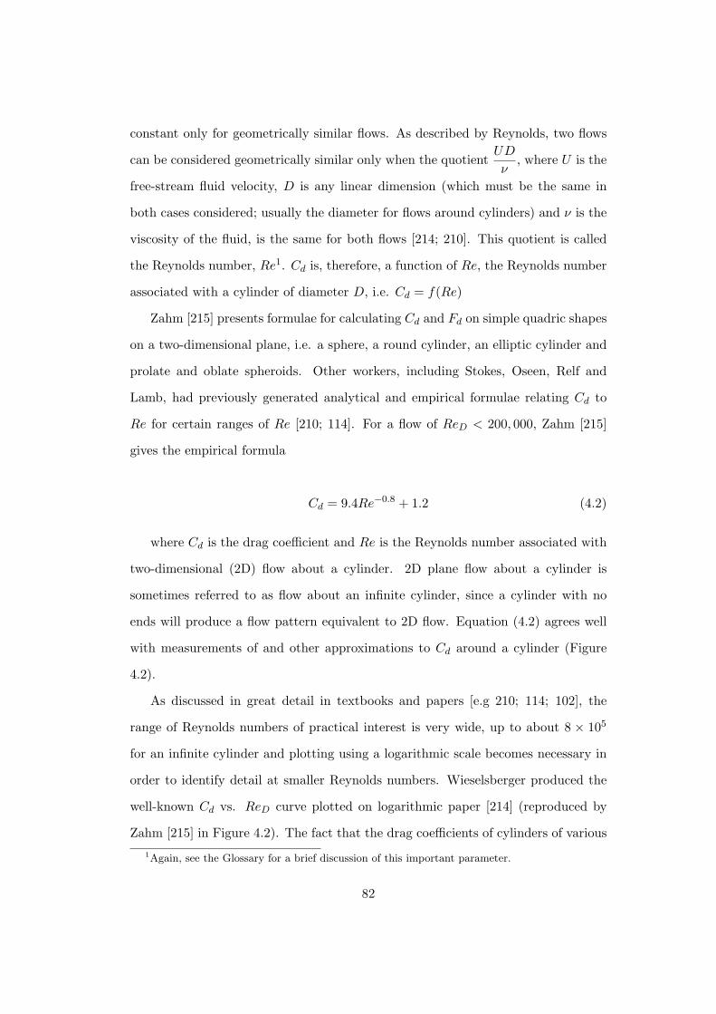
constant only for geometrically similar flows. As described by Reynolds, two flows

can be considered geometrically similar only when the quotientUD

ν, where U is the

free-stream fluid velocity, D is any linear dimension (which must be the same in

both cases considered; usually the diameter for flows around cylinders) and ν is the

viscosity of the fluid, is the same for both flows [214; 210]. This quotient is called

the Reynolds number, Re1. Cd is, therefore, a function of Re, the Reynolds number

associated with a cylinder of diameter D, i.e. Cd = f(Re)

Zahm [215] presents formulae for calculating Cd and Fd on simple quadric shapes

on a two-dimensional plane, i.e. a sphere, a round cylinder, an elliptic cylinder and

prolate and oblate spheroids. Other workers, including Stokes, Oseen, Relf and

Lamb, had previously generated analytical and empirical formulae relating Cd to

Re for certain ranges of Re [210; 114]. For a flow of ReD < 200, 000, Zahm [215]

gives the empirical formula

Cd = 9.4Re−0.8 + 1.2 (4.2)

where Cd is the drag coefficient and Re is the Reynolds number associated with

two-dimensional (2D) flow about a cylinder. 2D plane flow about a cylinder is

sometimes referred to as flow about an infinite cylinder, since a cylinder with no

ends will produce a flow pattern equivalent to 2D flow. Equation (4.2) agrees well

with measurements of and other approximations to Cd around a cylinder (Figure

4.2).

As discussed in great detail in textbooks and papers [e.g 210; 114; 102], the

range of Reynolds numbers of practical interest is very wide, up to about 8 × 105

for an infinite cylinder and plotting using a logarithmic scale becomes necessary in

order to identify detail at smaller Reynolds numbers. Wieselsberger produced the

well-known Cd vs. ReD curve plotted on logarithmic paper [214] (reproduced by

Zahm [215] in Figure 4.2). The fact that the drag coefficients of cylinders of various

1Again, see the Glossary for a brief discussion of this important parameter.

82

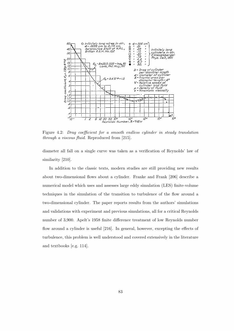
Figure 4.2: Drag coefficient for a smooth endless cylinder in steady translationthrough a viscous fluid. Reproduced from [215].

diameter all fall on a single curve was taken as a verification of Reynolds’ law of

similarity [210].

In addition to the classic texts, modern studies are still providing new results

about two-dimensional flows about a cylinder. Franke and Frank [206] describe a

numerical model which uses and assesses large eddy simulation (LES) finite-volume

techniques in the simulation of the transition to turbulence of the flow around a

two-dimensional cylinder. The paper reports results from the authors’ simulations

and validations with experiment and previous simulations, all for a critical Reynolds

number of 3,900. Apelt’s 1958 finite difference treatment of low Reynolds number

flow around a cylinder is useful [216]. In general, however, excepting the effects of

turbulence, this problem is well understood and covered extensively in the literature

and textbooks [e.g. 114].

83

4.3 Flow Around Finite Cylinders

The problem of a finite circular cylinder2 in cross-flow has also been extensively

studied because of the interesting complex flow phenomena it produces and because

of its importance in practical engineering [217; 218]. However, although the finite

cylinder is much studied, it is less well understood and new work still appears [219].

The primary references for flows about finite cylinders used in this thesis include

a paper by Park and Lee [204]. This is an experimental paper, and contains very use-

ful measurements and images of the flow about finite cylinders, of aspect or height

to diameter ratios (H/D) 6, 10 and 13, at a Reynolds number of 20,000. Complex

three-dimensional flow structures are observed in the wake of finite cylinders; these

structures are the result of quasi two-dimensional flow around the cylinder inter-

acting with axial flows. Although many factors contribute to the three-dimensional

behaviour of the wake flow, free end or tip-flow effects, resulting from flow over and

around the free end of finite cylinders, make the most significant contribution to

these axial flows [204]. The complexity of the wake structures is vividly demon-

strated by some experimental observations due to Park and Lee. The complexity

of the wake flow is corroborated and discussed in many other studies for various

Reynolds numbers [e.g. 220; 217].

The vortex formation length is defined as the distance from the lee-side of the

cylinder to the region of maximum velocity fluctuation in the cylinder wake and

has a value of about 2 for short cylinders3 of H/D < 10 and 1 for taller cylinders

H/D > 10 [220; 204]. The longer vortex formation region for cylinders of small

aspect ratio may be a result of the additional influence of the necklace vortex that

forms around the base section of a finite cylinder and which also contributes to the

three-dimensionality of the flow behind a finite cylinder [217]. For cylinders of small

aspect ratio (H/D < 6), the effect of flow around the free-end influences the wake

2i.e. a cylinder that does have ends.3Normalised with respect to the vortex formation length of a two-dimensional cylinder.

84

flow over the entire length of the cylinder, while for relatively long cylinders, the

free-end influence is confined to a region close to the free-end [220]. The tip-flow

effect on the base pressure coefficient4 increases with H/D for H/D < 7, and then

remaining constant for H/D ≥ 7 [218]. A particularly important observation is

that, aside from the wake region, the flow is essentially two-dimensional at a level

two diameters below the top of the cylinder [204].

This wake flow structure5 is observed at all Reynolds numbers [217]. The influ-

ence of the free-end and the base effects increases along the cylinder with increasing

Reynolds number and with decreasing aspect ratio.

Several experimental descriptions of the flow around a finite cylinder are in-

structive [204; 217]. When a flow approaches the free-end of a finite cylinder, the

flow moves upwards, accelerating around the free-end before separating from the

cylinder at the free end and forming a trailing vortex. This trailing vortex is pushed

downwards, influencing the wake behind the top half of the finite cylinder. The

wake behind the lower half of the cylinder is practically two-dimensional and not

influenced by the downwash.

4.4 Flow Around a Meteorological Tower

The meteorological mast studied was a 50 m high thin-walled tubular tower with

an outside diameter of 0.15 m. The tower was hollow, with a gap between its

base and the ground (Figure 4.1 (a)). The anemometer was located only 0.30 m

(two diameters) above than the top of the tower, close enough that wind-speed

measurements were likely to be affected by speed-up. In assessing the effect of

the tower on the anemometer, we studied various configurations of wind-speed,

4The base pressure coefficient Cpbcan be derived from Bernoulli’s equation, p +

1

2ρV

2 = const,

where ρ is the fluid density. This can be re-written as ps = p∞ + 1

2ρU2

∞(1 − 4sin2θ) for flow about

a cylinder. Cpbcan then be written, Cpb

=ps − p∞

1

2ρU2

∞

Cpb. See also Glossary.

5Suppressed two-dimensional flow around the mid-regions of the cylinder with significant three-dimensional effects at the free-end and close to the base.

85

turbulence and the slope of the local terrain. We also took into account the fact

that the tower was hollow. This model was built using the commercial computational

fluid dynamics (CFD) code Fluent [106], coupled with a simple analytical analysis.

Our objectives in this study were (i) to validate Fluent as a useful tool, in the

context of this work, and (ii) to approximate the velocity distortion at the top of a

finite cylinder using Fluent.

4.4.1 Validation

The purpose of our validation was to demonstrate that the results from Fluent

compare well with the experimentally observed flow structures and associated effects

of two dimensional laminar, steady and unsteady flow. The validation was both

qualitative and quantitative. Quantitatively, our aim was to approximate the drag

coefficient Cd and the pressure distribution Cp6.

We began by looking at the flow about an infinite, or two-dimensional, cylinder.

The validation consisted of running simulations for various Re and comparing the

results with experiment and theory [e.g. 212].

For the finite cylinder, the aim was to qualitatively replicate the flow pattern

above and around the cylinder as well as calculating Cd, and Cp at various heights

along the cylinder.

4.4.2 Meshing the Computational Domain

We experimented with various different grid geometries for both the two-dimensional

and three-dimensional simulations. In the two-dimensional case, three domain types

were tested, of rectangular, semi-circular and circular shape respectively. As de-

scribed earlier, these were inspired by reports, tutorials and papers from several

sources [e.g 106; 131; 221]. Various grid configurations were tested within each of

these three main domain types.

6See the Glossary for a brief discussion of this parameter.

86

Figure 4.3: The dense two-dimensional computational domain with the cylinderlocated in the very centre. The left edge is the inlet; the right edge is the outlet.

We considered an infinite cylinder of diameter, D = 2.0 m placed in a uniform

crossflow with a free-stream velocity of 1.0 m s−1. The inlet and outlet are 6.25D m

and 11.25D m respectively from the centre of the cylinder. The top and bottom of

the computational domain are equidistant from the cylinder centre and 8D m apart.

Semi-circular and circular domains most closely approximated the flow features of

interest to us (the circumferential pressure distribution and separation points, wake

configurations and drag coefficients).

In three dimensions, we again tested several domain types, each with more than

one internal grid configuration. Similar to the two-dimensional case, the three main

domain forms we considered were : a rectangular prism (a brick shape), a semi-

spherical domain, and a quarter-spherical domain. The quarter- and semi-spherical

domains were found to work best.

The Fluent model consisted of a quarter-sphere with a diameter 40 times that

of the cylinder. The cylinder represented the topmost ten diameters (H/D = 10)

of our met tower (H/D > 300). By considering the axial symmetry of flow around

cylinders, it was only necessary to model half the tower: this permitted use of

a dense mesh without leading to excessive computation time. The mesh for our

model contains approximately 650,000 tetrahedral cells, most of them close to the

tower. The half-cylinder was placed centrally.

87

4.4.3 Boundary and Initial Conditions

The properties of the fluid were assumed constant. In the two-dimensional simula-

tions, a no-slip7 wall condition is applied to the cylinder wall. Uniform free stream

conditions with varying degrees of turbulence are applied at the inlet (velocity inlet)

and lateral boundaries (symmetry). The flow exit is treated as a pressure outlet.

In the case of a solid three-dimensional tower, there are five boundary conditions.

At the bottom of the domain the flow is two-dimensional. The use of a symmetry

condition as the bottom face enforced this constraint. The flow symmetry about the

centre line of the cylinder allowed us to use another symmetry condition on the single

vertical surface. The tower itself was assigned a wall condition, implying zero wind-

speed at the surface. The upstream curved surface was defined as a velocity inlet.

This allowed us to specify the free-stream wind-speed and a turbulence intensity.

We defined the downstream face as a pressure outlet with atmospheric pressure.

The resulting model is shown in Figure 4.4.

A Fluent case file contains all the necessary inputs required by Fluent to specify

a particular problem. This includes the computational domain geometry (including

the grid), the boundary and initial conditions, the fluid properties, and the settings

of the various solution parameters (for example which turbulence model to use).

The fluid properties were set as constant with the boundary conditions described.

Fluent’s first-order discretisation scheme was used to model unsteady flows for Re >

50. It is important to note that the drag coefficient (Cd), is conventionally calculated

per diameter length of cylinder, as opposed to per unit length, for convenience.

4.4.4 Dimensional Analysis

Take axes centred at the top of the tower and define D (tower diameter), H (tower

height) and U (incident airspeed). Then, if we define u(z) to be the horizontal

7The no-slip wall condition is a central, simplifying observation used in boundary-layer theory.It states that there is no relative motion between a surface and that part of the fluid flow which isin contact with the surface.

88

velocity at a height z above the cylinder:

u(z)

U= f(z[m], D[m], H[m], ν[m2 s−1], ǫ[m], U [m s−1]) (4.3)

where ν and ǫ are the kinematic viscosity of air and the turbulence length scale of

the incoming airstream respectively. With some consideration, dimensional analysis

then gives us:

u(z)

U= F

(

z

D,UD

ν,H

D,ǫ

U

)

(4.4)

That is,u(z)

Uis some function, F, of four dimensionless groups. The dimension-

less groupUD

νis the Reynolds number (Re) of the flow and takes values in the

range of 10,000 to 100,000.H

Dcan be taken as approximately equal to 300. Since

the Reynolds number andH

Dare both >> 1, it is anticipated that

u(z)

Uis indepen-

dent of both these numbers. Flows become independent of Reynolds number when

Re is large. Similarly, for structures of H/D > 5, additional height does not affect

flow patterns about the free end(s). So,

u(z)

U= F

( z

D,ǫ

U

)

(4.5)

4.4.5 Modelling Turbulence

The turbulence intensity I is the ratio of the root-mean-square of the velocity fluc-

tuations, urms, to the mean flow velocity, u [117], thus:

I =urms

u(4.6)

This is the definition adopted by Fluent [106]. There is no one turbulence model

that is the best choice for all types of problem; the choice of turbulence model

depends on factors including the physics of the flow, conventions for dealing with

89

particular types of problem, the accuracy required and the resources available [106].

A careful weighing of these factors is required when choosing a turbulence model.

The Spalart-Allmaras (S-A) model was chosen for the wind energy work carried

out as part of the work presented in this thesis. This turbulence model is a good

choice where speedy results are required and accurate turbulent flow computations

are not required [106]. The S-A model is also suitable for relatively coarse grids since

it uses wall functions when the mesh resolution is not sufficiently fine. In the Fluent

implementation of the S-A model, the user is required to provide inlet boundary

conditions by setting the turbulence intensity and a turbulence length scale, based

on a representative dimension such as the diameter of a cylinder.

4.5 Modelling a Solid Tower

4.5.1 Some Considerations

In a previous study, it was shown that the flow around a finite cylinder at a height

of one diameter below the free-end is approximately two-dimensional; the speed-up

is not influenced by the airflow far below the top of the tower [204]. For this reason,

even though our tower had an aspect ratio of more than 300 (H/D > 300), it was

necessary only to model the topmost 1.5 m, or a cylinder of height to diameter ratio

10 (H/D = 10).

4.5.2 Calculating the Speed-up

On completion of a simulation run8, we recorded wind-speed values at specified

positions close to the free-end of the tower. These were located at 30 intervals,

on a circle congruent and concentric with the circumference and at a height of two

diameters above the top of the tower (Figure 7.8). These correspond to positions at

which the centre of the anemometer may be located. An actual anemometer consists

8One run comprises approximately 2,000 0.1 s time-steps, with 50 iterative computing steps ineach of them.

90

of three cups rotating on a fixed circular path around the centre of the device and

so the wind-speed is not measured exactly at the centre of the device but rather

on the path followed by the cups. From our simulations, however, we concluded

that the difference between the speed-up estimated at the centre of the anemometer

and the speed-up estimated on the circle followed by the cups is always less than

0.08% of the free-stream wind-speed. The wind-speed estimated at the centre of

the anemometer, therefore, represents an acceptable approximation to the values

recorded by an actual cup-device for the purposes of this study.

4.6 Modelling a Hollow Tower

4.6.1 Additional Considerations

The accelerating airflow around the top of the tower is at a lower pressure than

the still air at the bottom of the tower, next to the ground, where the pressure is

atmospheric. This sets up a pressure drop from the bottom to the top and gives rise

to an airflow up through the hollow centre of the tower. The velocity of this internal

airflow can be computed using the empirical Darcy-Weisbach equation [222], which

can be written

ω =

√

2D∆p

λHρ(4.7)

where ω is the speed of the airflow exiting through the top of the tower, ∆p is

the pressure drop from the bottom of the tower to the top, D is the diameter of the

tower, H its height, λ the pipe friction coefficient, calculated iteratively using the

Colebrook-White equation [222], and ρ is the air density.


The internal airflow through the hollow tower can be captured by changing the

top surface of the tower from a wall boundary to a velocity inlet. The air velocity

91

Figure 4.4: The computational domain with exploded surfaces for illustration.

assigned to this inlet is computed using an iterative process (Figure 4.5). Essentially:

(1) an initial run of the solid tower simulation provides a pressure value at the top of

the tower; (2) using this value to calculate ∆p in Equation (4.7), we then estimate

the internal airflow speed ω at the top of the tower; (3) we use this value for ω as the

top boundary condition for the next simulation run in order to get a new estimate

for the pressure drop; (4) this process is repeated until ω converges to a fixed value.

4.7 Modelling a Tower on Sloped Terrain

4.7.1 Additional Considerations

We assumed that in the vicinity of the free-end of a tower positioned vertically on a

hill, the airflow is parallel to the slope of the hill and has a turbulence intensity close

to that of flat terrain. Turbulence intensity is defined as the ratio of the root-mean-

square of the velocity fluctuations, u′, to the mean flow velocity, u [117]. Although

92

Figure 4.5: The iterative process used to calculate the speed-up over a hollow tower.The process is repeated until ω converges to a fixed value.

the vertical component of turbulence intensity does change on encountering the

windward side of a hill [223; 224; 225], this mechanism is not relevant to our study.

In addition, as we report later in this thesis, speed-up is not sensitive to changes in

turbulence intensity.


We need only change the inlet and bottom face boundary conditions. Airflow now

enters through the inlet and bottom faces, inclined at an angle to the horizontal

equal to the terrain slope.

In addition to speed-up, there are other sources of measurement error associated

with anemometers. One source of error, relevant to this thesis, results from the fact

that anemometers only measure the wind velocity component perpendicular to the

main axis of the device, which is almost always vertical; this has implications for a

met tower sited vertically on the windward side of a hill, subject to an uphill wind

that is parallel to the slope. In this thesis, the speed-up error can be understood as

93

both the speed-up error in the actual absolute flow velocity above the vertical tower

and the speed-up error in the velocity reported by the anemometer.


In this chapter describes the literature, theory and methods related to the second

of the three studies that contribute to this thesis were presented. The results from

this work are presented in Chapter 7 with a discussion of their utility and how

they contribute to the thesis that simulation is useful. Chapter 5 continues with a

description of the third of the three studies presented in this thesis.

94

Chapter 5

Literature Review, Theory and

Methods, Study 3

The third part of the work presented in this thesis concerns one possible end state for

a dissolving tablet: fragmentation into small particles with dissolution continuing

from the disintegrated solid masses. A framework for calculating the motion of, and

dissolution from, a drug particle moving through the USP apparatus is outlined,

beginning with a review of the classical work of Taylor and Glauert [22; 23], who

considered the motion of raindrops in airflows. This chapter presents the literature,

theory and methods relevant to this third study.

5.1 Describing Particle Motion in a Fluid

In 1940, G.I. Taylor outlined, with great clarity of thought, a methodology for

determining the two-dimensional equations of motion of raindrops moving in curved

airstreams [22]. This work was to facilitate the design of a suitable wind tunnel for

carrying out de-icing experiments. In this paper, Taylor presented the exact solution

for the paths of raindrops moving in a jet impinging on a flat plate, the flow close

95

to a stagnation point1, when Stokes’ law of resistance2 is assumed to apply. Taylor

defines the two-dimensional equations of motion for a raindrop in a fluid which is

moving with velocity components u and v as:

4

3πa3du1

dt=

1

2πCdρa

2q(u− u1)

4

3πa3dv1

dt=

1

2πCdρa

2q(v − v1)

where Cd is the drag coefficient of a sphere,

q =(

(u− u1)2 + (v − v1)

2) 1

2 , u1 and v1 are the velocity components of the drop, 2a

its diameter, its density and ρ the density of air. With the assumption of Stokes

flow, these equations can be written in a simplified form. In general, the equations of

motion must be solved numerically. In 1940, before the advent of modern computing,

Glauert calculated the paths of the particles using an unspecified step-by-step, or

numerical, integration method [23].

Glauert further applied Taylor’s technique to the problem of ice accumulation

on a two-dimensional circular cylinder and an airfoil. Using the equations of motion

for Stokes flow developed by Taylor, Glauert hand-computed two-dimensional paths

for raindrops of different sizes moving around various simple shapes. The combined

work of Taylor [22] and Glauert [23] forms an excellent introduction to particle

tracking in a fluid, i.e. simple two-phase flow.

Several related NACA papers were also published at that time and a subsequent

paper by Bergrun provides a very useful expansion on the techniques described

by Glauert, applied to a NACA airfoil [226]. In particular, Bergrun discusses the

case when the raindrop departs from Stokes flow. In this case, the equations of

1When a fluid flow impinges on a surface, e.g. perpendicularly onto a flat plate, the middlestream-line will come to rest at a point on the surface. This is a stagnation point [see e.g. 193].

2Stokes flow or creeping flow assumes that the density, or inertia, terms are all negligible inthe equations of motion. It can be shown by non-dimensionalising the Navier-Stokes momentumequation that this assumption is valid only for very small Reynolds numbers [193; 210; 114].

96

motion solved by Glauert must be modified to account for a continuously variable

drag coefficient, Cd. Assuming that the acceleration of the particle is constant over

the time-step, Bergrun outlines an integration method using a linear first order

approximation for velocity and a second order approximation for position; taking

the x -direction:

upn+1 = up

n + apn∆t+O(h)

xpn+1 = xp

n + upn∆t+ ap

n∆t2 +O(h2)

This amounts to using the Euler integration method to calculate new velocities

and positions. Since the velocity values are only O(h) accurate, the accuracy in the

calculation of positions is not as good as the theoretical O(h2). Bergrun also presents

a method of estimating the initial relative difference, or differentials between the

particle and flow velocities which are required to initiate the calculations. A later

paper contains further useful derivations associated with particle motion about an

airfoil [227].

In more recent years, refinements in computing and mathematical descriptions

have led to significant progress in particle tracking capabilities. Nevertheless, the

basic mathematical descriptions of and methodologies for Eulerian/Lagrangian3 cal-

culations of particle motion through an aerodynamic or hydrodynamic field have

not changed very much in a broad sense [229]. The paths of the particles moving

through the velocity field are calculated by numerical integration of variations of

the equations of motion. For example, additional forces may need to be included

[e.g. 230]. In the general case, the velocity field is too complex to be calculated

3Eulerian descriptions of two-phase flows consider effects relative to a fixed point in space whileLagrangian descriptions describe the effects relative to the reference frame of a particular particlemoving through the fluid. In the Eulerian description of motion, the velocity vi is defined in termsof x, y, z, t, i.e. u(x, y, z, t), v(x, y, z, t), w(x, y, z, t) while in the Lagrangian system, xA(t), yA(t)and zA(t) are specified for each fluid particle. In general, Lagrangian computational models havegrid points that move with the fluid, while Eulerian grid points remain fixed in space [228].

97

analytically and instead fluid velocity values at a finite number of discrete points

are computed using a numerical computational fluid dynamics (CFD) code, such

as the commercial code Fluent. The resulting structured or unstructured matrix

of velocity data, associated with the CFD grid points, is then used to calculate the

motion of the particle. For a steady velocity field, which is assumed to be unaffected

by the motion of the particle, the particle position is first located in the grid. If

the particle is not at a grid point, velocity information from surrounding grid points

must be interpolated to find the fluid velocities at the particle location. Using this

information, the equations of motion must be integrated to determine the position

of the particle at the next time-step. This new position must then be located in the

data set and the process starts over again.

5.2 Governing Equations

As outlined above, one version of the two-dimensional equations of motion for a

spherical drop in a steady stream with velocity components u and v are [22]:

4

3πa3du1

dt=

1

2πCdρa

2q(u− u1) (5.1)

4

3πa3dv1

dt=

1

2πCdρa

2q(v − v1) (5.2)

where, as described above, Cd is the drag coefficient, q =(

(u− u1)2 + (v − v1)

2) 1

2 ,

u1 and v1 are the velocity components of the drop, 2a its diameter, its density and

ρ the density of the fluid. If x and y are the coordinates of the drop at time t, then

dx

dt= u1,

dy

dt= v1

98

Figure 5.1: With the basic equations of motion, FInertia =d

dt(mv) and Fd = ma,

where m is the mass of the particle, v its velocity and a in this context its acceler-ation, there is a balance between the inertia and drag forces.

5.3 Forces

We can readily see that the left hand side of Equations (5.1) and (5.2), the inertial

force, arise from Newton’s Second Law (Figure 5.1). The right hand side of Equa-

tions (5.1) and (5.2) describe the drag force acting on a particle moving through

a fluid. In reality, the drag coefficient Cd varies continuously with the Reynolds

number Rep of the particle in the flow4. Rep is given by:

Rep =2aq

ν(5.3)

[210]. Cd can be considered constant, however, in certain situations, such as

when the Rep is large. In other situations, e.g. when the Rep is very small, the

relationship between Cd and Rep can be approximated as linear [see e.g. 210].

If the particles are assumed to be very small, Stokes’ law of resistance can be

applied5. In this case, the drag coefficient, CdStokes:

CdStokes=

24

Rep

4See the Glossary for a discussion of the Reynolds number.5Strictly, Stokes’ law only applies when a flow is very slow, very steady and when the boundary

walls are very far away [231].

99

[210] and ν is the kinematic viscosity of the fluid. It follows that CdStokes=

12ν

aq

and, in terms of u and v, Equations (5.1) and (5.2) then simplify to

K0d2x

dt2+dx

dt− u = 0 (5.4)

K0d2y

dt2+dy

dt− v = 0 (5.5)

where

K0 =2

9

ρ

a2

ν(5.6)

Stokes flow pertains when Rep << 1. In the majority of cases, Stokes’ law does

not apply, e.g. when the particle is relatively large. We observe that, in general

[226]:

Cd = CdStokes× f(Rep) (5.7)

where Cd is the drag coefficient written in its most general form, f() is a function

of Rep and is based on the empirical formulae given by Loth [232]. We can write

that Cd = CdStokes× f(Rep) =

12ν

aq× f(Rep). Simplifying Equations (5.1) and (5.2)

using Cd instead of CdStokesyields

CfK0d2x

dt2+dx

dt− u = 0 (5.8)

CfK0d2y

dt2+dy

dt− v = 0 (5.9)

with variables as defined previously and the correction factor, Cf =1

f(Rep). The

correction to the Stokes flow solution for a continuously variable Cd is calculated

using Loth’s empirical formulas [232]:

100

• Rep <= 1, Cf = 1 + 316

(Rep).

• Rep > 1 and Rep <= 285, Cf = 1 + 0.1935Rep0.6305.

• Rep > 285 and Rep <= 2, 000, Cf = 1 + 0.015Rep + 0.2283Rep0.43.

• Rep > 2, 000 and Rep <= 3, 500, 000, Cf = 0.44Rep24

.

• Rep >= 3, 500, 000, Cf = 0.44Rep24

.

Equations (5.1) and (5.2) represent a useful description of particle motion in a

fluid. However, as outlined by other workers [e.g. 230], other forces act on a particle

in a flow. For small Rep, Equation (5.1) can be written in a more general way as:

(mp +1

2mf )

du1

dt= (mp −mf )g +

3

2mf

du

dt+

1

2πCdρa

2q(u− u1) + FHistory (5.10)

where the mf terms are added mass terms, used to capture the resistance of the

fluid to acceleration. FHistory, the history term, accounts for the effect the particle

has on the velocity field. These additional forces, including the effect of gravity g, are

ignored by Taylor since they are relatively small for particles the size of raindrops.

For the same reasons, they are not included in the analysis presented here.

5.4 Computer Implementation of Particle Motion in a

Two-Dimensional Flow Near the Stagnation Point

Taylor and Glauert’s results for solution of the two-dimensional equations of motion

of raindrops moving in curved airstreams [22; 23] provide a useful comparison for

testing the various components of a numerical model of the motion of particles

in flows. Taylor presents the exact solution for the case of particle motion close

to a stagnation point when Stokes’ law of resistance applies. This solution was

101

implemented numerically and extended in this thesis for the general case when

Stokes’ law does not apply.

5.4.1 Taylor’s Exact Solution

As outlined by Taylor [22], the velocity field close to a stagnation point is given

by u = −cx, v = cy. If these values for u and v are substituted into the general

equations of motion, Equations (5.4) and (5.5), the resulting equation may be non-

dimensionalised by substituting z = t/K0, α = K0c. This gives

d2x

dz2+dx

dz+ αx = 0 (5.11)

d2y

dz2+dy

dz− αy = 0 (5.12)

Taylor presents exact solutions to Equations (5.4) and (5.5) for various values

of α for a particle travelling with the stream at z = t = 0. These provide a useful

benchmark for numerical implementations.

5.4.2 Review

To calculate the paths of the particles moving through the velocity field, the discrete

versions of Equations (5.11) and (5.12) are integrated using a Runge-Kutta method.

A generalised particle tracking process is: (1) Calculate the fluid velocities at time

t at a finite number of grid points, (2) Search the grid to find the fluid velocities at

the position of the particle, (3) Interpolate data from the grid points closest to the

particle to determine the fluid velocities at its location, (4) Integrate the equations

of motion using these velocities and determine the new particle position, and (5)

Analyse and/or visualise the resulting data. For unsteady flows, this process must

be completed for each time-step. For steady flows, it is necessary to perform step

(1) only once.

102

For the case of a particle moving in a two-dimensional flow near the stagnation

point, the algorithm is as follows: (1) Define the fluid flow as u = −cx and v = cy,

where x and y are the coordinates of the particle at time t; (2) Define the flow

velocities u = −cxt=0 and v = cyt=0. This is the initial position of the particle.

From the assignment on the previous page, at t = 0, z = t = 0 ; (3) define the

Reynolds number Rep,t=0 of a stationary particle at xt=0, yt=0 (this is discussed in

more detail overleaf) ; (4) integrate the transformed equations of motion, Equations

(5.11) and (5.12), using a fourth order Runge-Kutta method; (5) For the general

case, Cd is calculated at each time-step.

5.4.3 Methods

G.I. Taylor’s 1940 paper was the starting point for this research [22]. The technique

described in this paper for the treatment of a particle motion in the case of a jet

impinging on a flat plate, summarised above, was implemented on the computer6

using step-by-step techniques, similar to those used by Glauert [23].

5.4.4 Evaluation of the Drag Force

The drag force is calculated at each time-like z-step and at the intermediate Runge-

Kutta stages. When Stokes’ law of resistance applies, the numerical solution of

Equations (5.11) and (5.12) agrees well with Taylor’s exact solution. In the general

case where Stokes law does not apply, Equations (5.13) and (5.14) are modified

following the procedure outlined in Section 5.3, giving:

Cfd2x

dz2+dx

dz+ αx = 0 (5.13)

Cfd2y

dz2+dy

dz− αy = 0 (5.14)

6Using the Python scripting language.

103

with the Cf already defined.

5.4.5 Initial Conditions

Two extreme situations at t = 0 were considered: (1) the particle is moving with

the flow and (2) the particle is at rest relative to the flow. Solutions were calculated:

(i) for the special case when Stokes’ law applies, using Equations (5.11) and (5.12)

and (ii) for the general case when Stokes’ law does not apply, using Equations (5.13)

and (5.14).

5.4.6 Evaluation of the Relative Reynolds Number, Rep

In terms of z, the initial relative Reynolds number of the particle with respect to

the flow can be written

Rep =2aq(z)

K0ν=

2acq(z)z,t=0

αν

using Equations (5.3) and (5.6). As mentioned, the two extreme initial conditions

are (1) the particle is moving with the flow at z = t = 0 and (2) the particle is at

rest with respect to the flow at z = t = 0. For convenience, z and t are taken to

be the same quantity in the following discussion; in Taylor’s work, the calculations

proceed in terms of z and a routine conversion is used to express them in terms of t.

Taking initial condition (2) first, the particle is initially at rest and qt=0 = 0. qt=0 is

the relative or resultant velocity between the particle and the fluid at t = 0. Since α

and qt=0 are known, setting Rep,t=0 to some reasonable value automatically defines

a, the radius of the particle (from Equation (5.3) and the definition of K0). From

descriptions in the preceding pages, it can be understood that the definition of α

and a automatically set c, the constant of proportionality between the flowspeed

and the displacement along the x or y axis; a sets K0 and α and K0 together set

c. Rep,t=0 and α are, it follows, the defining quantities for this analysis. Once

these values are set, the calculations can then proceed with Cd recalculated at each

104

time-step.The Reynolds number at each new time-step t+ ∆t can calculated using

Rep(t + ∆t) = q(t + ∆t)Rep(t)

q(t). This arises from the definition of the Reynolds

number, i.e. q is the only quantity that varies when a particle of constant size

moves through a fluid of constant viscosity.

With initial condition (1), when the particle is moving with the fluid at t = 0,

a similar consideration applies: if α and Rep are both specified at t = 0, and given

that q(z)p,t=0 is a function of α only, a and c are automatically defined, again using

Equation (5.3) and Section 5.4.1.

This presents a problem, however. At t = 0 there is no relative movement

between the fragment and the fluid flow and Rep,t=0 = 0. There is not enough

information to allow calculation of Rep at subsequent time-steps using the procedure

outlined above. In order to get around this problem and to kick-start the simulation,

the Reynolds number for the same particle standing still relative to the fluid must

be defined at t = 0; this is an additional input to the simulation. In addition, the

initial resultant velocity qt=0 between a stationary particle and the fluid is calculated.

From the definition of the Rep on the previous page, it can be seen that knowledge

of Rep,t=0, qt=0 and α automatically defines the product ac, i.e. a measure of the

product of particle size and flow velocity. A large Rep,t=0 corresponds to a fast flow

and/or a large raindrop. Conversely, a small Rep,t=0 corresponds to a slow flow

and/or a small raindrop. Using these values for Rep,t=0 and qt=0 allow initialisation

of the simulation; calculations for subsequent time-steps are not affected.

5.4.7 Generating the Numerical Grid

A structured numerical grid for the 2D stagnation flow was generated using a simple

code which calculated the velocity values u and v at a selected number of points

x0, y0 to xN , yN using the exact solution (u = −cx and v = cy). The evenly spaced

N ×N grid was written to a text file in the format shown in Table 5.1.

Additional text files were generated with node and element connectivity infor-

105

Node x y u v

N1 0.0 0.0 0.0 0.0

N2 0.0 1.4 0.0 0.7

N3 0.0 2.9 0.0 1.4

...

NN 0.0 4.3 0.0 2.1

Table 5.1: The format of the structured numerical grid used in the numerical im-plementation of Taylor’s work. N1 to NN are the node labels.

mation. For a 4 × 4 grid, nodes and elements were numbered from the bottom left

hand corner to the top right hand corner.

5.4.8 Localisation and Interpolation

Review

Calculating a particle trajectory using Eulerian or Lagrangian methods involves lo-

calisation, i.e. finding the particle position x relative to the surrounding grid points.

This is straightforward for a structured cartesian grid, where the grid is aligned

with the reference frame [229]. Locating a particle in unstructured grids, however, is

generally computationally intensive [229; 233]. Since unstructured grids are increas-

ingly used by computational fluid dynamics codes to mesh complex geometries and

since the particle-locating, or localisation, algorithm must be performed after each

simulation time-step, an efficient algorithm is essential. This is particularly true for

simulations of many particles featuring complex flow phenomena such as turbulence

[229].

In an Eulerian description of a two-phase flow, the carrier velocity and other

flow variables are known at a discrete number of grid points. The function of the

localisation algorithm is to find the carrier velocity and other relevant flow variables

at the particle position [229]. This involves two steps: (i) locating the particle in

106

the grid, identifying the grid cell that it belongs to at a particular time and (ii)

interpolating information from the surrounding grid points to calculate the carrier

velocity and flow variables of interest at the particle position [229].

Many localisation algorithms have been designed. The simplest general locali-

sation method involves calculating and comparing the Euclidean distance between

p and each node in the grid. The fluid p(x, y) is assigned the velocity values of

the closest node. This is known as nearest neighbour interpolation. Lohner out-

lines a simple brute-force search algorithm for a single particle in an unstructured

grid consisting of either two-dimensional triangular elements or tetrahedral three-

dimensional elements using shape functions7 [234]. This technique can be applied

to any cell shape by reorganising the cells into triangles or tetrahedra. Due to its

simplicity, this algorithm is very fast. In addition, it is readily vectorised 8. Other

more advanced search and interpolation techniques are discussed by Zhou [229] and

Chodra [233].

Methods

In order to find the fluid velocities at any point p(xp, yp), the point must be located

in the numerical grid. Once located, the values for the fluid velocities at the point are

estimated using one or more values associated with the surrounding grid points. The

first search and interpolate method we used was the simple nearest neighbour scheme

where the Euclidean distance between p and each node in the grid is calculated and

compared. p(x, y) is assigned the velocity values of the closest node, Nc. The 2D

Euclidean separation δn is calculated as

δn =√

(xn − xp)2 + (yn − yp)2

7In the one-dimensional case, where a cell or element consists of a line joining two points, a andb, a variable u defined at a and b can be interpolated from its value at a and b. The expression is

u =

(

xb − x

xb − xa

)

ua +

(

x − xa

xb − xa

)

ub. The quotients in brackets are referred to as shape functions.

Similar expressions can be derived for two-dimensional and three-dimensional elements.8Vectorising allows efficient, parallel operation on vector-like quantities.

107

Figure 5.2: USP Dissolution Apparatus 2 generated from CGNS data provided byDeirdre D’Arcy at the School of Pharmacy in Trinity College Dublin [19]. Visualisedfor this thesis using VisIt [235].

where xn and yn are the x and y co-ordinates of the grid point under consider-

ation.

5.5 Particle Motion in the USP Apparatus

The core work presented earlier in this thesis considered the initial drug dissolution

from a dissolving compact using numerical techniques, providing good agreement

with experimental results for relatively slowly dissolving systems over short disso-

lution times. One possible end state of a tablet is that, at some stage, it breaks

up with dissolution occurring from the disintegrated solid masses. The end-point of

the work begun in this thesis is to provide simulations for (i) longer time periods of

dissolution and (ii) disintegrating and particulate systems. In addition to some of

the techniques already discussed, a first step towards objective (ii) is to examine an

existing CFD simulation of the USP apparatus.

108

5.5.1 USP Apparatus Data

The velocity field within the USP Dissolution Apparatus was produced by D’Arcy

et al [19] using the commercial CFD code Fluent. The Fluent model is of the

entire USP dissolution apparatus and does not make use of any device symmetries.

It is certainly possible that some symmetry considerations could have been used

to reduce computation; however, it is understood that the intention was to create

a faithful representation of the device. The Fluent hydrodynamic simulation was

exported in ASCII and ADF (Advanced Data Format) as specified by the CFD

General Notation System (CGNS) [236; 237]. In order to reduce the large ASCII

text file to a manageable size for plotting, a Python script was used to thin the data.

The script steps through the data file, keeping only every nth line of data [238].

5.5.2 Integration of the Equations of Motion

Numerical integration of ordinary differential equations is concerned with solving

initial value problems of the form y′ = f(x, y), y(a) = y0 over a ≤ x ≤ b. Rather

than providing a solution to y′ = f(x, y) at every x, numerical methods provide

solutions at a finite, preselected set of x values [239], where x is the time-like variable.

This results in tables of values for x and y. These tables of values, nowadays

calculated by computer and potentially containing a very large amount of data, are

generally graphed to facilitate interpretation of the results. Numerical solutions can

provide information where algebraic expressions cannot [239].

There are very many integration methods including the (Fundamental) Euler

Method or Point Slope Method and its variations, the Trapezoidal Method, the

Leap-Frog or Half-Step Method (all linear approximations). Other methods include

Adam’s Interpolation and Extrapolation methods, the Runge-Kutta Method, Gill’s

Method, Predictor-Corrector Methods, the Feynman Method and the Verlet Method

[see 240; 239; 241; 242]. The Runge-Kutta Method, strictly a family of methods

which includes the Heun Method, is one of many multi-stage algorithms. Multi-stage

109

Figure 5.3: The Euler integration method is a simple linear approximation to theparticle trajectory. Many time-steps are needed to ensure a basic level of accuracy.x, u and a represent the position, velocity and acceleration values at a point.

methods require calculations at intermediate steps in the time-like sense [243]. Many

other methods and variations of existing methods have been devised [244; 242].

Numerical methods should provide accurate and stable solutions that can be

performed in a reasonable time with reasonable resources. A series of informative

educational papers published in the American Journal of Physics provided insight

into various integration techniques [241; 244; 245; 246; 247; 248; 242]. Although

discussed in detail in many textbooks [e.g. 240; 239], three of the most important

methods are described here. Different methods are suitable for different problems;

Runge-Kutta methods are commonly used when high accuracy is required. The

Verlet method is popular and provides a compromise between accuracy and speed.

Euler methods have a low accuracy but are very fast.

Euler or Point Slope Method

The simplest integration method for the solution ofdy

dx= f(x, y), y(x0) = y0 is the

linear Point Slope or Euler Method [239]. Given a starting position P (x0, y0) and

a slope f(x0, y0), the aim is to find y0 ... yn corresponding to x0 ... xn. Taking a

tangent through the curve at P0, the tangent may be a good approximation to the

actual curve in a very small interval around x0, say in the range x0 − h to x0 + h,

110

where h is some small value. Moving along the curve from P0 to P1, it is possible

then to write x1 = x0 + h and y1 = y0 + hf(x0, y0). The Euler Method has a

discretisation error O(h2) for each step in the time-like direction. For the system

u =dx

dt= f(x, t), x(t0) = x0 (Figure 5.3), we can write xn+1 = xn + un∆t. This

equation represents a particle’s position with time. u in turn can be calculated from

the equation un+1 = un + an∆t, where an is the acceleration at n.

Although attractive for its simplicity, the error accumulates with each step of

the time-like direction and quickly becomes significant rendering the solution too

inaccurate for use. Other linear algorithms such as the Mid-point Method and the

Leap-Frog or Half-Step Method have much better accuracy [241]. It is interesting to

note that according to Cromer [241], the superior accuracy of the Leap-Frog Method

over the Euler Method is not because it better approximates the first derivative at

a point, but because it better approximates the first integral of motion.

Runge-Kutta Methods

As outlined in textbooks [e.g. 240; 239], one particular Runge-Kutta method consists

of four intermediate calculations to solve for y in y′ = f(x, y). The solution is:

yn+1 = yn +1

6k1 +

1

3k2 +

1

3k3 +

1

6k4 +O(h5) (5.15)

Where values are as defined previously and k1 = hf(xn, yn), k2 = hf(xn +

12h, yn + 1

2k1), k3 = hf(xn + 1

2h, yn + 1

2k2) and k4 = hf(xn + h, yn + k3).

Runge-Kutta methods, although accurate, incur calculation and storage penal-

ties, requiring calculation of the variables at intermediate positions between steps in

the time-like direction and can result in a computationally expensive program [249].

Nevertheless, Runge-Kutta methods are widely used [e.g. 250; 251; 252].

111

Verlet Method

The Verlet method was used by Loup Verlet in his 1967 paper on the motion of

particles under the influence of molecular forces [110]. The Verlet algorithm and its

variants are widely used in physics engines where high-speed calculation is necessary.

Verlet solves md2ridt2

=∑

j 6=i

f(ri,j) using:

ri(t+ h) = 2ri(t) − ri(t− h) +∑

j 6=i

f(ri,j(t))h2 (5.16)

where h is a small time increment. The Verlet algorithm is derived by combining

two Taylor series expansions. With r the position, v the velocities, a the accelera-

tions, and b the third derivatives of r with respect to t, all vector quantities, we can

write:

r(t+ ∆t) = r(t) + v(t)∆t+ ...+ a(t)∆t2 + (1/6)b(t)∆t3 +O(∆t4) (5.17)

r(t− ∆t) = r(t) − v(t)∆t+ ...+ a(t)∆t2 − (1/6)b(t)∆t3 +O(∆t4) (5.18)

Adding Equations (5.17) and (5.18) gives

r(t+ ∆t) = 2r(t) − r(t− ∆t) + 2a(t)∆t2 +O(∆t4)

Which is the method proposed by Verlet. The Verlet algorithm is accurate,

formally of O(∆t4) though no third derivatives are explicitly required. It is simple

to implement and is popular. Velocity values can be calculated using

v(t) =r(t+ ∆t) − r(t− ∆t)

2∆t+O(∆t2)

112

The disadvantage of this is that the error in the velocity values are O(∆t2) rather

than O(∆t4). Swope et al. showed that the velocity values at the new time-step

can be explicitly calculated with a higher accuracy by re-writing the algorithm in

an equivalent form [253], yielding:

r(t+ ∆t) = r(t) + v(t)∆t+1

2a(t)∆t2 (5.19)

v(t+ ∆t) = v(t) −1

2

(

f(t+ ∆t) + f(t))

∆t (5.20)

However, this requires knowledge of the force or accelerations at t + ∆t before

calculation of the velocities at t + ∆t, i.e. the forces acting on the body must be

known at t+ ∆t.

5.6 Preliminary Analysis of Particle Motion in the USP

Apparatus

5.6.1 Typical Particle Size

Assuming Stokes flow, the drag force (Fd) on a sphere can be written Fd = 6πµaU , or

Fd

µaU= 6π = const. [114]. The momentum of a particle is written as p =

4

3πa3ρpU .

Since F = ma, we can write F ≈p

t, or t ≈

43πa3ρpU

For t ≈

43πa3ρpU

6πµaU=

2a2

9ν.

Taking the time to destroy the momentum of a particle as being about 1 second

and the kinematic viscosity of the fluid to be that of the solvent, 0.1M HCl at 37o,

i.e. ν = 0.00786 ≈ 10−2 cm2 s−1, then 1 ≈ 100a2 or a ≈ 0.1 cm. The important

parameter in this approximation is the time taken for a particle initially at rest to

achieve the same velocity as the fluid, i.e. 1 second in the estimate presented.

113

0.00

0.05

0.10

0.15

0.20

Flu

id V

eloc

ity M

agni

tude

(m

/s)

Grid Points

Figure 5.4: Fluid velocity magnitudes encountered within the USP Dissolution Ap-paratus 2. As can be clearly seen, velocities are distributed mostly between 5 cms−1 and 10 cm s−1. The average fluid velocity magnitude within the device is about7.2 cm s−1.

5.6.2 Maximum Fluid Velocities

With a paddle speed of about 50 revolutions per minute, or5

6revolutions per second,

the maximum tangential speed for fixed body rotation at the edges of the device

will be5

6× 2πr = 31.4 cm s−1. For a particle at rest with respect to the device, the

maximum relative velocity will therefore be 31.4 cm s−1.

5.6.3 Maximum Relative Reynolds Number, Rep

With qmax = 31.4 cm s−1, a = 0.05 cm and ν = 0.00787 ≈ 10−2 cm2 s−1, Rep =

2aqmax

ν=

31.4 × 0.1

10−2≈ 800. With q = 1.83 cm s−1, taken from previous studies

[17], Rep ≈ 46. The average fluid velocity magnitude within the device is about 7.2

cm s−1 (Figure 5.4), giving Rep =7.2 × 0.1

0.00787≈ 91.4.

5.6.4 Effect of Discrete Velocity Field Density on the Relative

Reynolds Number, Rep

The original discrete velocity fields, produced by D’Arcy et al [19], were processed to

produce several additional files containing subsets of the original data. These subsets

114

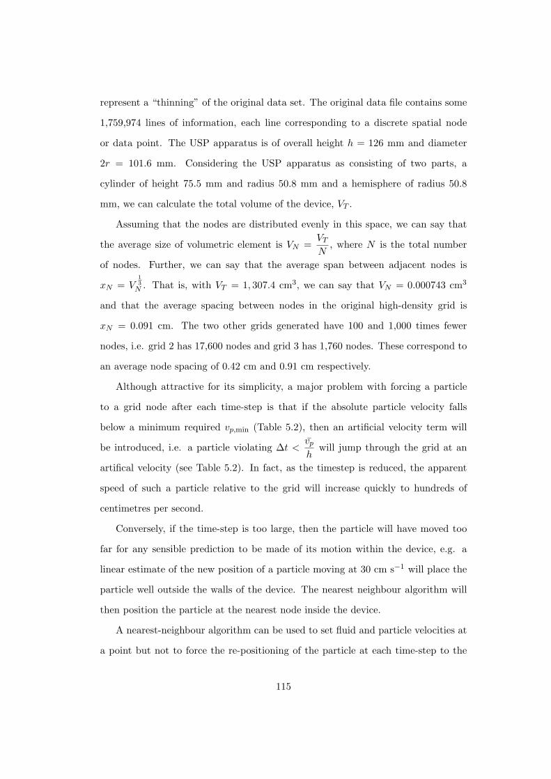
represent a “thinning” of the original data set. The original data file contains some

1,759,974 lines of information, each line corresponding to a discrete spatial node

or data point. The USP apparatus is of overall height h = 126 mm and diameter

2r = 101.6 mm. Considering the USP apparatus as consisting of two parts, a

cylinder of height 75.5 mm and radius 50.8 mm and a hemisphere of radius 50.8

mm, we can calculate the total volume of the device, VT .

Assuming that the nodes are distributed evenly in this space, we can say that

the average size of volumetric element is VN =VT

N, where N is the total number

of nodes. Further, we can say that the average span between adjacent nodes is

xN = V13

N . That is, with VT = 1, 307.4 cm3, we can say that VN = 0.000743 cm3

and that the average spacing between nodes in the original high-density grid is

xN = 0.091 cm. The two other grids generated have 100 and 1,000 times fewer

nodes, i.e. grid 2 has 17,600 nodes and grid 3 has 1,760 nodes. These correspond to

an average node spacing of 0.42 cm and 0.91 cm respectively.

Although attractive for its simplicity, a major problem with forcing a particle

to a grid node after each time-step is that if the absolute particle velocity falls

below a minimum required vp,min (Table 5.2), then an artificial velocity term will

be introduced, i.e. a particle violating ∆t <vp

hwill jump through the grid at an

artifical velocity (see Table 5.2). In fact, as the timestep is reduced, the apparent

speed of such a particle relative to the grid will increase quickly to hundreds of

centimetres per second.

Conversely, if the time-step is too large, then the particle will have moved too

far for any sensible prediction to be made of its motion within the device, e.g. a

linear estimate of the new position of a particle moving at 30 cm s−1 will place the

particle well outside the walls of the device. The nearest neighbour algorithm will

then position the particle at the nearest node inside the device.

A nearest-neighbour algorithm can be used to set fluid and particle velocities at

a point but not to force the re-positioning of the particle at each time-step to the

115

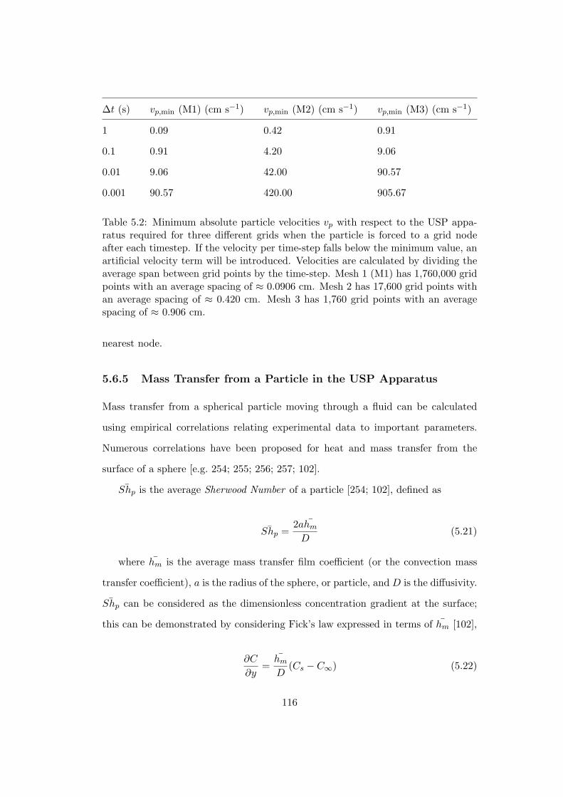
∆t (s) vp,min (M1) (cm s−1) vp,min (M2) (cm s−1) vp,min (M3) (cm s−1)

1 0.09 0.42 0.91

0.1 0.91 4.20 9.06

0.01 9.06 42.00 90.57

0.001 90.57 420.00 905.67

Table 5.2: Minimum absolute particle velocities vp with respect to the USP appa-ratus required for three different grids when the particle is forced to a grid nodeafter each timestep. If the velocity per time-step falls below the minimum value, anartificial velocity term will be introduced. Velocities are calculated by dividing theaverage span between grid points by the time-step. Mesh 1 (M1) has 1,760,000 gridpoints with an average spacing of ≈ 0.0906 cm. Mesh 2 has 17,600 grid points withan average spacing of ≈ 0.420 cm. Mesh 3 has 1,760 grid points with an averagespacing of ≈ 0.906 cm.

nearest node.

5.6.5 Mass Transfer from a Particle in the USP Apparatus

Mass transfer from a spherical particle moving through a fluid can be calculated

using empirical correlations relating experimental data to important parameters.

Numerous correlations have been proposed for heat and mass transfer from the

surface of a sphere [e.g. 254; 255; 256; 257; 102].

¯Shp is the average Sherwood Number of a particle [254; 102], defined as

¯Shp =2ahm

D(5.21)

where hm is the average mass transfer film coefficient (or the convection mass

transfer coefficient), a is the radius of the sphere, or particle, and D is the diffusivity.

¯Shp can be considered as the dimensionless concentration gradient at the surface;

this can be demonstrated by considering Fick’s law expressed in terms of hm [102],

∂C

∂y=hm

D(Cs − C∞) (5.22)

116

Sink conditions pertain, since it is assumed that the initial particle weight is

less than 10 % of the amount of solute necessary to saturate the solution [88], so

C∞ ≈ 0, and

∂C

∂y=hm

D(Cs) (5.23)

Non-dimensionalising this equation by multiplying∂C

∂yby

2a

Csyields,

∂c′

∂y′=

2ahm

D(5.24)

where∂c′

∂y′is the dimensionless concentration gradient at the surface and, as

previously shown, the group2ahm

Dis the average Sherwood number. When ¯Shp is

known, a value for the mass transfer from a particle in a fluid can be calculated by

writing

hm = −DAB

2a¯Shp (5.25)

Since the average mass flux of solute per unit surface area of the sphere is given

by

m′′ = −hmCs (5.26)

assuming sink conditions, the mass transfer rate from a spherical particle of

radius a can is then calculated as

m = −4πa2hmCs = −2aπDAB¯ShpCs (5.27)

The Sherwood number of, and hence mass transfer from, a spherical particle is a

function of three main processes, (i) radial diffusion, (ii) free or natural convection

and (iii) forced convection. These processes are linked to the Schmidt number (Sc),

117

Grashof number (G′) and Reynolds number (Rep) respectively. Sc and Rep are

well known9. The Grashof number, G′, can be considered as the free convection

equivalent of the Reynolds number, and is a measure of the ratio of the inertial

forces to the buoyancy forces [254; 102]. G′ is defined as

G′ =8ga3

ν2

∆ρ

ρ(5.28)

where g is acceleration due to gravity, a is the radius of the particle, ν is the

kinematic viscosity of the solvent, ρ is the bulk density of the pure solvent and ∆ρ

is the difference between the density of the saturated solution and the bulk density.

For the problem under consideration, g = 980 cm s−2, a varies with particle

size, and the properties of pure 0.1M hydrochloric acid (HCl) are ν = 7.87 × 10−3

cm2 s−1, ρ = 1.19 g cm−3. D’arcy et al. arrived at an experimental value for ∆ρ

of 1.99 kg m−3 or 1.99 × 10−3 g cm−3 [258]. Other relevant quantities include the

saturation concentration of benzoic acid in HCl, Cs = 4.55 × 10−3 g cm−3 and the

diffusivity D = 1.236 × 10−5 cm2 s−1. The Schmidt number, Sc =ν

D= 636.7.

Using these values, together with the average relative Reynolds numbers, Rep,

calculated for particles of various sizes moving through the USP apparatus, we can

determine G′. Experimental correlations are chosen to relate ¯Shp to these three

numbers. Once ¯Shp is known, the average mass transfer rate m can be calculated

Garner [254] and Miller [257] provide reviews of useful experimental correlations

although more recent studies also exist. Well-known correlations include those of

Ranz and Marshall and Harriott [255; 256]. Incropera and DeWitt recommend a

heat transfer correlation proposed by Whitaker in 1972 [102]. The work presented

here uses four recommended correlations, two each from Garner and Miller for free

and forced convection respectively. ¯Shp = 2 corresponds to mass transfer by radial

diffusion only and represents the lower limit of ¯Shp [254].

These correlations are: (1) Garner’s free convection correlation,

9See the Glossary for brief descriptions.

118

¯Shp = 0.50(G′Sc)0.25 (5.29)

for G′Sc ≤ 105. (2) Garner’s forced convection correlation,

¯Shp = 0.50(G′Sc)0.25 + 0.48Re0.5p Sc0.33 (5.30)

again for G′Sc ≤ 105. (3) Miller’s free convection correlation,

¯Shp = 2 + 0.60G′0.25Sc0.25 (5.31)

(4) Miller’s forced convection correlation,

¯Shp = 2 + 1.10Re0.5p Sc0.33 (5.32)

Using these correlations, hm can be calculated as described previously, i.e. m =

−2aπDABShpCs.

Miller’s 1971 paper is a very useful review of mass transfer correlations for sus-

pended solute particles dissolving in an agitated vessel [257]. Importantly, Miller

reports that radial diffusion is the dominant mode of mass transfer for particles of

diameter 205 microns and less, based on data presented by Harriott in his 1962 work

[255]. This figure was arrived at by considering the turbulence microscale measure

η which represents the size of the smallest turbulent eddies expected in a particular

system configuration. As discussed by Miller, η (as defined by Shinnar and Church

an earlier 1960 paper) is given as:

η = 0.1983(P/V ′)−14 ν

34 (5.33)

where P is the agitator power input and V ′ is the volume of the device. Eddies

at the small eddy equilibrium end of the turbulence energy spectrum are most

important for mass transfer [257].

119

5.6.6 Visualisation of Results

With the development of CFD, the visualisation of the complex data produced by

these codes has become increasingly important. Visualisation greatly facilitates

the interpretation of complex data, revealing underlying patterns and structures

[259]. All the information presented graphically in this thesis is visualised using

GnuPlot [189], VisIt [235], Fluent [106] or ADFViewer [260]. GnuPlot, the standard

Unix/Linux tool, was used to produce most of the two-dimensional plots while

Fluent, ADFViewer and VisIt were used to visualise the commercial CFD code

data.


This chapter introduced the literature, theory and methods associated with the third

study that contributes to this thesis, the dissolution of a drug particle moving in the

USP apparatus. This included a review of the classical work of Taylor and Glauert,

who calculated analytical and numerical solutions to the motion of raindrops in

curved airstreams. The governing equations for, and an overview of the numerical

methods involved in, the calculation of particle motion in the USP apparatus were

described. The chapter finishes with some preliminary ideas about expected particle

motion and a review of experimental mass transfer correlations. The utility of the

methods presented here and their relevance to the thesis, that simulation is useful

for pharmaceutics, is discussed in Chapter 8. Chapter 6 continues with results, and

discussion, about the first of the three studies described.

120

Chapter 6

Results and Discussion, Study 1

In this chapter we present results from the core investigations presented in this thesis,

i.e. the initial dissolution rate from a tablet dissolving in the USP apparatus. The

significance of these results, as well as their context in the overall thesis, is discussed.

6.1 Investigations of Previous Work

6.1.1 The Pohlhausen Solution

As discussed previously, Crane et al. [17] describe a semi-analytical procedure for

calculating the release rate of drug, m, from a cylindrical tablet that consists of

alternating layers of drug and excipient, concluding with several expressions that

can be used to get solutions for tablets consisting, in total, of 3 and 5 layers. Two

questions immediately come to mind: (1) can these expressions be generalised to

deal with any number of layers and (2) what happens when the number of layers

is very large? Does the drug release rate as predicted by Crane et al. tend to a

limiting value?

121

Generalising to Many Layers

Considering the expression given by Crane et al. for the ratio of the mass transfer of

an excipient from a 3-layer compact (me-3-layer) to the mass transfer from a compact

consisting entirely of the excipient (me-1-layer),

me-3-layer

me-1-layer

=

[

1 −

(

x2

x3

) 34

+

(

x1

x3

) 34

]23

(6.1)

where x1, x2 and x3 are defined for 1-/3-layer systems in Figure 3.1, it becomes

evident that, for the case of a compact consisting of 3 equally-spaced layers, one

drug layer sandwiched between two layers of excipient, we can replace this equation

with the equivalent expression

me-3-layer

me-1-layer

=

[ 2∑

n=0

(

3 − n

3

) 34

(−1)n

] 23

(6.2)

Likewise, and for the same condition of 3 equally-spaced and alternating layers,

its complement, the ratio of the mass transfer of a drug from a 3-layer compact

(md-3-layer) to the mass transfer from a compact consisting entirely of the drug

(md-1-layer) can be written as

md-3-layer

md-1-layer

=

[

1 −2

∑

n=0

(

3 − n

3

) 34

(−1)n

] 23

(6.3)

Similarly for the case of five equally spaced and alternating layers of drug and

excipient, two drug layers sandwiched between three layers of excipient

me-5-layer

me-1-layer

=

[ 4∑

n=0

(

5 − n

5

) 34

(−1)n

] 23

(6.4)

md-5-layer

md-1-layer

=

[

1 −4

∑

n=0

(

5 − n

5

) 34

(−1)n

] 23

(6.5)

We can at this point easily generalise these observations to an odd number, p,

122

of equally-spaced, alternating, layers of drug and excipient with the drug layers

sandwiched between the layers of excipient:

me-p-layer

me-1-layer

=

[p−1∑

n=0

(

p− n

p

)i

(−1)n

] 23

(6.6)

md-p-layer

md-1-layer

=

[

1 −

p−1∑

n=0

(

p− n

p

)i

(−1)n

] 23

(6.7)

where i is the index, evaluated as 34

[17]. These equations represent an extension

of the work of Crane et al [17]. We explicitly state the general case that their results

imply.

The Case When the Number of Layers is Large

It can be readily demonstrated that the series appearing in Equation (6.6) converges

to a fixed value as p → ∞ for the case of i = 1. When i = 1, the series can be

written as −0

p+

1

p−

2

p+

3

p−

4

p+

5

p...

p

p. Pairing the terms as follows,

(

−0

p+

1

p

)

+(

−2

p+

3

p

)

+

(

−4

p+

5

p

)

+ ... +

(

−(p− 1)

p+

5

p

)

, it is evident that the sum of

these pairs is always1

p. Since there are

(p+ 1)

2differences, the series sums to

1

p×

(p+ 1)

2=

1

2+

1

2p.

As p becomes large,1

2pbecomes small and the sum of the series converges to

1

2.

The question now becomes, what is the behaviour of Equation (6.6) as p → ∞ for

positive values of i other than 1? Taking the case when i is an integer, i ∈ Z, we

can write that

p−1∑

n=0

(

p− n

p

)i

(−1)n =1

pi

[

pi − (p− 1)i + (p− 2)i − (p− 3)i + ...]

.

Since xi − yi = (x − y)(xi + xi−2y + ... + yi) and if we group the terms in pairs,

denoted as 2n and 2n− 1 where n = 1, ... ,p

2, we can re-write this series as

123

p−1∑

n=0

(

p− n

p

)i

(−1)n =

1

pi

p

2∑

n=0

(

2n− (2n− 1))(

(2ni−1) + 2ni−2(2n− 1) + ...+ (2n− 1)i−1)

Since 2n− (2n− 1) = 1,

p−1∑

n=0

(

p− n

p

)i

(−1)n =1

pi

p

2∑

n=1

1.(

i(2n)i−1 + terms with power i− 2 or less)

=1

pi

p

2∑

n=1

(

i(2i−1)ni−1 + terms with power i− 2 or less)

=1

pii2i−1

p

2∑

n=1

(

(ni−1) + terms with power i− 2 or less)

Using the identityn

∑

k=1

kΓ =nΓ+1

Γ + 1+(terms with powers less than Γ + 1), we can

write

p−1∑

n=0

(

p− n

p

)i

(−1)n =1

pii2i−1

(

pi

i2i+ terms with power i− 1 or less

)

=1

2+

(

terms that are functions of1

p

)

=1

2as p→ ∞

The next step is to investigate the behaviour of Equation (6.6) as p → ∞ for

positive values of i other than i ∈ Z, i.e. for i a rational number, i ∈ Q. Using

numerical experiments, it is clear that as p gets very large the sum of the series

approaches1

2for all i > 0 (Table 6.1). In addition, the ratio of the mass transfer

124

0.40

0.45

0.50

0.55

0.60

0.65

0.70

0.75

0.80

0.85

0.90

0.95

1.00

1.05

1.10

1.15

1.20

1 3 5 7 9 11 13 15 17

Mas

s T

rans

fer

Rat

e (m

g/m

in)

Number of Layers, n

Pohlhausen (Crane et al., 2004)

Finite Difference, N1/2 = 500



Figure 6.1: Mass transfer values calculated using the semi-analytical Pohlhausenmethod [21] and the numerical finite difference method presented in this thesis[261].

of a drug from a p-layer compact (md-5-layer) to the mass transfer from a compact

consisting entirely of the drug (md-1-layer) tends to

(

1

2

) 23

= 0.63 for all i > 0 as p

gets very large (see also Figure 6.1). Following the method proposed by Crane et

al [17], a tablet consisting of a very large number of alternating layers of drug and

excipient will have an (initial) mass transfer rate of drug equivalent to 63% of the

initial mass transfer rate of drug from a tablet that consists entirely of drug.

It is interesting to speculate on the possible applications of this solution. A

tablet containing a very large number of alternating layers of drug and excipient may

have similar initial dissolution properties to the more common type of dissolution

controlled tablet where small particles of drug and excipient are intermixed.

6.1.2 The PSUDO Solutions

The Effect of Advection Velocities on Mass Transfer Rates

As discussed in Chapter 2, the models used in the PSUDO project consistently

overestimate the mass transfer rate of drug from a layered compact [20]. The authors

125

i 0.25 0.75 1 2 3 4p3 0.8562 0.7009 0.6667 0.6667 0.7407 0.81485 0.8078 0.6319 0.6000 0.6000 0.6480 0.6960101 0.6400 0.5118 0.5050 0.5050 0.5074 0.50991,001 0.5786 0.5020 0.5005 0.5005 0.5007 0.501010,001 0.5442 0.5003 0.5000 0.5000 0.5001 0.5001100,001 0.5248 0.5001 0.5000 0.5000 0.5000 0.50001,000,001 0.5140 0.5000 0.5000 0.5000 0.5000 0.500010,000,001 0.5079 0.5000 0.5000 0.5000 0.5000 0.5000100,000,001 0.5044 0.5000 0.5000 0.5000 0.5000 0.50001,000,000,001 0.5025 0.5000 0.5000 0.5000 0.5000 0.5000

Table 6.1: Numerical investigation into the convergence of

p−1∑

n=0

(

p− n

p

)i

(−1)n for

i ∈ Q as p becomes large.

attribute this to the fact that mixing in the bulk fluid is neglected, so drug is not

drawn away from the surface sufficiently quickly. From examination of the literature,

it seems likely that the reasons for this overestimate are (1) the use of a constant

advection velocity vz in the boundary-layer region and (2) neglecting the normal

velocity vn.

In order to test these ideas and to ascertain the impact of these simplifications,

the Crank-Nicolson finite difference scheme was used to calculate the mass transfer

rate from tablets with a constant horizontal and vertical fluid velocity imposed across

the region of interest (i.e. the velocity boundary-layer was ignored). It is clear from

Table 6.2 that assuming a constant horizontal advection velocity vz throughout the

diffusion layer introduces a significant error into the calculation. In fact, the mass

transfer from a surface can be overestimated by more than a factor of 5. Neglecting

advection normal to the surface also introduces a smaller, but noticeable, error (See

Table 6.2). One direct result of the over-estimated fluid velocity close to the surface

is that the concentration boundary-layer will tend to stay close to the surface with

time. In addition, as noted in the report, the drug release profile will plateau much

too early.

126

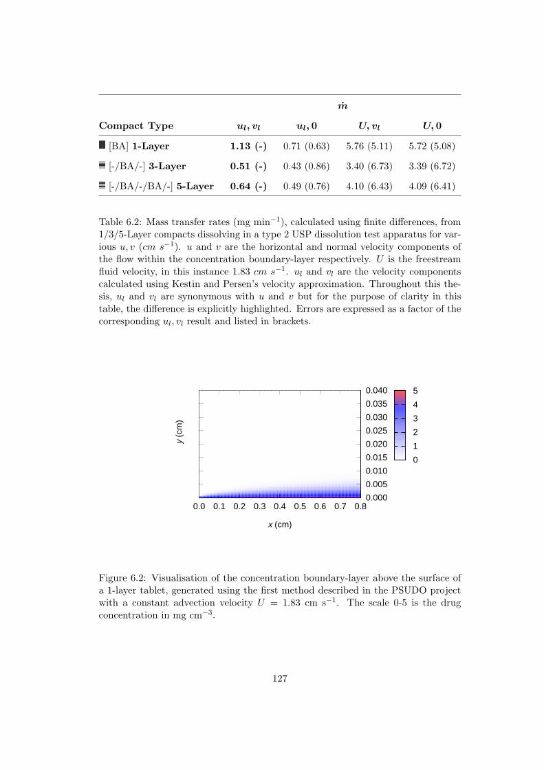
m

Compact Type ul, vl ul, 0 U, vl U, 0

[BA] 1-Layer 1.13 (-) 0.71 (0.63) 5.76 (5.11) 5.72 (5.08)

[-/BA/-] 3-Layer 0.51 (-) 0.43 (0.86) 3.40 (6.73) 3.39 (6.72)

[-/BA/-/BA/-] 5-Layer 0.64 (-) 0.49 (0.76) 4.10 (6.43) 4.09 (6.41)

Table 6.2: Mass transfer rates (mg min−1), calculated using finite differences, from1/3/5-Layer compacts dissolving in a type 2 USP dissolution test apparatus for var-ious u, v (cm s−1). u and v are the horizontal and normal velocity components ofthe flow within the concentration boundary-layer respectively. U is the freestreamfluid velocity, in this instance 1.83 cm s−1. ul and vl are the velocity componentscalculated using Kestin and Persen’s velocity approximation. Throughout this the-sis, ul and vl are synonymous with u and v but for the purpose of clarity in thistable, the difference is explicitly highlighted. Errors are expressed as a factor of thecorresponding ul, vl result and listed in brackets.

0

1

2

3

4

5

0.0 0.1 0.2 0.3 0.4 0.5 0.6 0.7 0.80.000

0.005

0.010

0.015

0.020

0.025

0.030

0.035

0.040

y (

cm)

x (cm)

Figure 6.2: Visualisation of the concentration boundary-layer above the surface ofa 1-layer tablet, generated using the first method described in the PSUDO projectwith a constant advection velocity U = 1.83 cm s−1. The scale 0-5 is the drugconcentration in mg cm−3.

127

In the visualisation of the concentration boundary-layer above the surface of

a 1-layer tablet shown in Figure 6.2, the fluid is moving from left to right and

the surface of the tablet forms the bottom axis of the graph. The visualisation is

generated using the first method described in the PSUDO project with a constant

advection velocity U = 1.83 cm s−1. The normal velocity component is neglected.

The resulting high mass transfer rate of 9.53 × 10−5 g s−1 (or 5.72 mg min−1) is

vividly apparent in the thin concentration boundary-layer.

0

1

2

3

4

5

0.0 0.1 0.2 0.3 0.4 0.5 0.6 0.7 0.80.000

0.005

0.010

0.015

0.020

0.025

0.030

0.035

0.040

y (

cm)

x (cm)

Figure 6.3: Visualisation of results from the finite difference scheme outlined in thisthesis with a freestream velocity of U = 1.83 cm s−1. u and v close to the surfaceare calculated using the velocity boundary-layer equations.

The second visualisation (Figure 6.3) was generated using the finite difference

method presented in this thesis with a freestream velocity of U = 1.83 cm s−1

[261]. The velocity components close to the surface are calculated in accordance

with boundary-layer theory. The resulting mass transfer rate of 1.13 mg min−1 is

consistent with analytical solutions and experiment presented later in this chapter.

The concentration boundary-layer can be seen to be obviously thicker due to the

lower velocities very close to the surface.

128

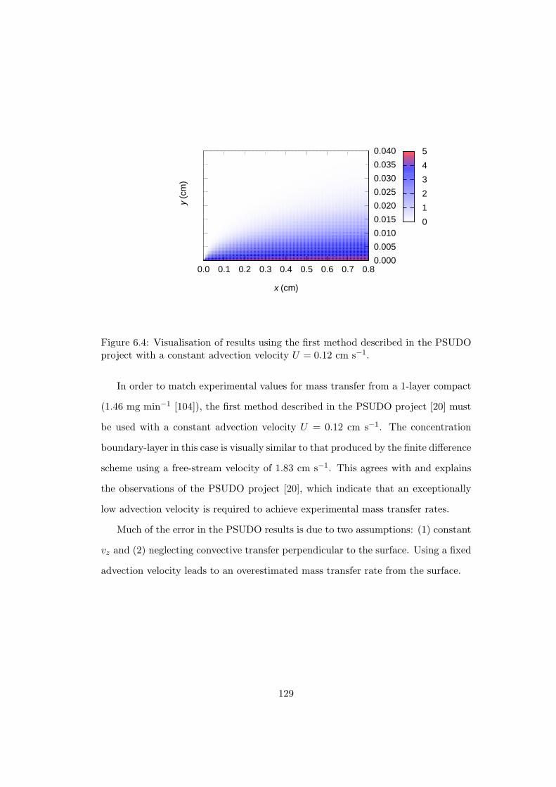
0

1

2

3

4

5

0.0 0.1 0.2 0.3 0.4 0.5 0.6 0.7 0.80.000

0.005

0.010

0.015

0.020

0.025

0.030

0.035

0.040

y (

cm)

x (cm)

Figure 6.4: Visualisation of results using the first method described in the PSUDOproject with a constant advection velocity U = 0.12 cm s−1.

In order to match experimental values for mass transfer from a 1-layer compact

(1.46 mg min−1 [104]), the first method described in the PSUDO project [20] must

be used with a constant advection velocity U = 0.12 cm s−1. The concentration

boundary-layer in this case is visually similar to that produced by the finite difference

scheme using a free-stream velocity of 1.83 cm s−1. This agrees with and explains

the observations of the PSUDO project [20], which indicate that an exceptionally

low advection velocity is required to achieve experimental mass transfer rates.

Much of the error in the PSUDO results is due to two assumptions: (1) constant

vz and (2) neglecting convective transfer perpendicular to the surface. Using a fixed

advection velocity leads to an overestimated mass transfer rate from the surface.

129

1.20

1.40

1.60

1.80

2.00

2.20

2.40

2.60

2.80

3.00

3.20

0.00020.00040.00060.00080.00100.00120.00140.00160.00180.0020

Log 1

0(R

untim

e) (

s)

h

1-Layer3-Layer5-Layer

Figure 6.5: Finite difference P4 2.4GHz 500MB RAM program runtimes with de-creasing representative cell size, h.

6.2 Numerical Results

6.2.1 Verification of the Scheme

A grid sensitivity analysis [144] (Table 6.3) indicated that the 5-layer finite difference

model converges as h → 0 with a discretisation error of 0.02 % (Table 6.4). The

1-layer finite difference scheme converges linearly with decreasing h, i.e. as follows

, as does the 5-layer scheme, i.e. as follows . The 3-layer scheme,

however, displays an oscillatory convergence, i.e. . These analyses give us

further confidence that the Crank-Nicolson finite difference scheme is solving the

equations correctly.

The finite difference program runtime can be defined as tc = βh2 where tc is the

computation time and β is a constant. tch=0.001 = 75 s (implemented with Python

on a 2.4 GHz P4, 512 MB RAM) where h is the cell size, defined earlier. So tc is a

simple function of the square of the cell size or a linear function of the number of

cells in the grid (Figure 6.5).

130

6.2.2 The Effect of Discontinuities

Leading Edge Velocity Singularity

For a 1-layer tablet of benzoic acid, the mass transfer rate m calculated using the

finite difference scheme is 1.1259 mg min−1 corrected for the velocity singularity

at the leading edge. The relative error with respect to the experimental value

of 1.46 mg min−1 [104] is 22.9% (Table 6.5). The mass transfer rates calculated

without a correction for the velocity singularity is 1.1299 mg min−1 (the singular

values at the leading edge were simply omitted). This has a 22.6% error with

respect to experiment and a 0.36% error with respect to the corrected solution. It

is interesting to note that the error between the corrected and uncorrected finite

difference solutions is small and that the uncorrected solution is still within 0.1% of

the Kestin-Persen analytical solution.

Crank-Nicolson Oscillations

As illustrated in Figure 6.6 a-f, our solution features discontinuities in the normal

first derivative of concentration at the edges of the diffusing regions. The calculated

∂c

∂y

∣

∣

∣

∣

y=0

oscillates in the streamwise direction, from left to right. This is a typical re-

sponse of the Crank-Nicolson scheme to sharp initial transients (the x or streamwise

direction is the time-like variable in our simulation) [157; 262; 198]. Although the

oscillations in∂c

∂y

∣

∣

∣

∣

y=0

clearly persist over the length of the diffusing regions (Figure

6.6 a-f), they are damped and are relatively small at the end of each of the regions.

In addition, as is evident in Figures 6.7 and 6.8, the oscillations in∂c

∂y

∣

∣

∣

∣

y=0

do not

lead to similar oscillations in c (with only minor distortions visible in Figure 6.8).

Taking the case of the finite difference solution for the 3-layer system, which is vali-

dated against an analytical solution (Table 6.5), the relative error between the finite

difference and the analytical solution is extremely small, much less than 0.01%. This

is well inside what is considered to be an acceptable level of accuracy in numerical

131

(a) 50 × 50 grid, 3-layer tablet.

(c) 200 × 200 grid, 3-layer tablet.

(e) 500 × 100 grid, 5-layer tablet.

(b) 100 × 100 grid, 3-layer tablet.

(d) 500 × 500 grid, 3-layer tablet.

(f) 500 × 500 grid, 5-layer tablet.

Figure 6.6: Discontinuities in∂c

∂y

∣

∣

∣

∣

y=0

, indicated by extreme values, occur at the

edges of the diffusing regions, resulting in oscillations of the Crank-Nicolson results.

simulation [136]. This is despite the oscillations in∂c

∂y

∣

∣

∣

∣

y=0

evident in Figure 6.6 a-d.

For this reason, although the extreme values of∂c

∂y

∣

∣

∣

∣

y=0

lead to oscillations in the

132

0.000.10

0.200.30

0.400.50

0.600.70

0.800.000

0.0050.010

0.0150.020

0.0250.030

0.0350.040

0.0

0.5

1.0

1.5

2.0

2.5

3.0

3.5

4.0

4.5

Concentration (mg cm-3)

x (cm)y (cm)

Concentration (mg cm-3)

Figure 6.7: Reverse angle visualisation of the concentration gradients above thesurface of a 5-layer tablet. The tablet surface is on the right of this plot and thefluid flow is from bottom right to top left. The high concentrations close to the two

diffusing layers are clearly visible. Crank-Nicolson oscillations in∂c

∂y

∣

∣

∣

∣

y=0

do not lead

to oscillations in c.

133

calculation of∂c

∂y

∣

∣

∣

∣

y=0

across the diffusing regions, the concentration values display

smooth behaviour.

0.0

0.5

1.0

1.5

2.0

2.5

3.0

3.5

4.0

4.5

0.00 0.10 0.20 0.30 0.40 0.50 0.60 0.70 0.80

Con

cent

ratio

n (m

g cm

-3)

x (cm)

Figure 6.8: Concentration vs. x position. Contours are lines of constant y. Thisplot is generated from a 200 × 200 grid. Some minor oscillation is visible at highconcentrations close to the leading edges of the diffusing regions (x = x1 and x = x3).

6.2.3 Validation, Comparison with Experiment and Previous Work

The good agreement between the finite difference method and the other models for

1-/3-layer compacts, suggests that the scheme is correctly describing the physics of

dissolution (Table 6.5).

It is clear from Figure 6.1 and Tables 6.5 and 6.6 that results from the finite

difference solution and the Pohlhausen solution of Crane et al. [17] diverge for

systems of 5 layers and more. However, the solutions diverge more slowly as the

number of layers increases. This behaviour is intuitive: the rate of increase in error

between the two solutions ought to fall as the number of layers increases. The

134

0.0

0.1

0.2

0.3

0.4

0.5

0.6

0.7

0.8

0.9

1.0

0.000 0.005 0.010 0.015 0.020 0.025 0.030 0.035 0.040 0.045

Nor

mal

ised

Con

cent

ratio

n

Normal Distance from Surface (Tablet Diameters)

Finite Difference Model

Crane et al. (2004a)

Figure 6.9: Concentration-distance curve normal to the compact surface at thestart of the inert layer, x = x2. The concentration curve for the Pohlhausen modelwas generated using an equivalent numerical implementation of the semi-analyticalPohlhausen model.

0.0

0.1

0.2

0.3

0.4

0.5

0.6

0.7

0.8

0.9

1.0

0.000 0.005 0.010 0.015 0.020 0.025 0.030 0.035 0.040 0.045

Nor

mal

ised

Con

cent

ratio

n




Figure 6.10: At the end of the inert region, at x = x3. The finite difference curve isthe more physically realistic.

135

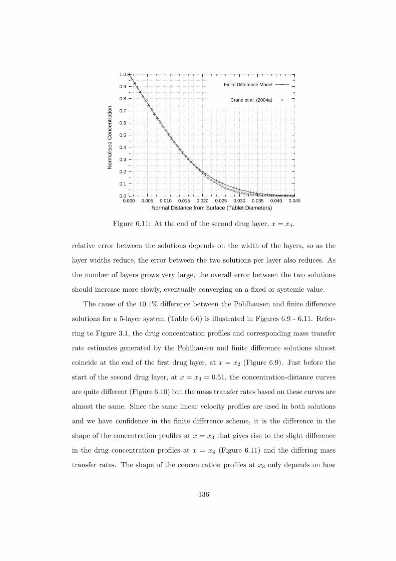
0.0

0.1

0.2

0.3

0.4

0.5

0.6

0.7

0.8

0.9

1.0

0.000 0.005 0.010 0.015 0.020 0.025 0.030 0.035 0.040 0.045

Nor

mal

ised

Con

cent

ratio

n




Figure 6.11: At the end of the second drug layer, x = x4.

relative error between the solutions depends on the width of the layers, so as the

layer widths reduce, the error between the two solutions per layer also reduces. As

the number of layers grows very large, the overall error between the two solutions

should increase more slowly, eventually converging on a fixed or systemic value.

The cause of the 10.1% difference between the Pohlhausen and finite difference

solutions for a 5-layer system (Table 6.6) is illustrated in Figures 6.9 - 6.11. Refer-

ring to Figure 3.1, the drug concentration profiles and corresponding mass transfer

rate estimates generated by the Pohlhausen and finite difference solutions almost

coincide at the end of the first drug layer, at x = x2 (Figure 6.9). Just before the

start of the second drug layer, at x = x3 = 0.51, the concentration-distance curves

are quite different (Figure 6.10) but the mass transfer rates based on these curves are

almost the same. Since the same linear velocity profiles are used in both solutions

and we have confidence in the finite difference scheme, it is the difference in the

shape of the concentration profiles at x = x3 that gives rise to the slight difference

in the drug concentration profiles at x = x4 (Figure 6.11) and the differing mass

transfer rates. The shape of the concentration profiles at x3 only depends on how

136

the Neumann boundary condition within the central layer (x2 ≤ x ≤ x3) is imple-

mented. It follows then that the 10.1% difference between the Pohlhausen and finite

difference estimates can be entirely attributed to the differing implementations of

this boundary condition. Further, the fixed relative error between the Pohlhausen

and finite difference estimates (Figure 6.1) can also be entirely attributed to the

different implementations of this same boundary condition.

Although the absolute theoretical and experimental mass transfer rate estimates

differ (Table 6.5), if the 3-/5-layer results are presented as fractions of the associated

1-layer solutions, a much better agreement is evident (Table 6.6). This suggests

that much of the underlying physics has been captured by the models. Recent

hydrodynamic analyses [44; 19] show that for a compact placed centrally in the

device the fluid flows tangential to the curved surface, not parallel to its long axis.

One implication of this, corresponding with our results, is that the theoretical models

will consistently underestimate the mass transfer rate. Any complete model of

drug dissolution will need to incorporate, in addition to the velocity boundary-layer

equations, a more realistic free-stream velocity, [e.g. 44; 19].

The results presented in this section were for layered tablets in which benzoic

acid (BA) is treated as the drug component. Previous studies [104; 21; 17] provide

graphed data for layered tablets in which salicylic acid is the drug component, i.e.

the 1-layer compact consists entirely of BA and the 3- and 5-layer tablets have the

form BA/SA/BA and the BA/SA/BA/SA/BA respectively. Graphing output from

the finite difference model (Figure 6.12) and comparing it with graphs from Crane

et al. [21] (Figure 6.13), we can see that the initial mass transfer rates calculated

with the finite difference model agree reasonably well with the previous studies and

with experiment.

137

0

50

100

150

200

250

0 50 100 150 200 250

SA 3-Layer

SA 5-Layer

Figure 6.12: Finite difference showing dissolved mass of Salicylic Acid (SA) againsttime (minutes).

Figure 6.13: Results for compacts of BA and SA, showing dissolved mass of each sub-stance against time. The 3-layer and 5-layer compacts have reversed structures whencompared to the tablets for which results are presented in this thesis. Reprinted from[17], copyright (2004), with permission from Elsevier.


In summary, this chapter presented results from the first of three studies described

in this thesis.

The Pohlhausen [17] and PSUDO [20] models of the initial mass transfer rate

138

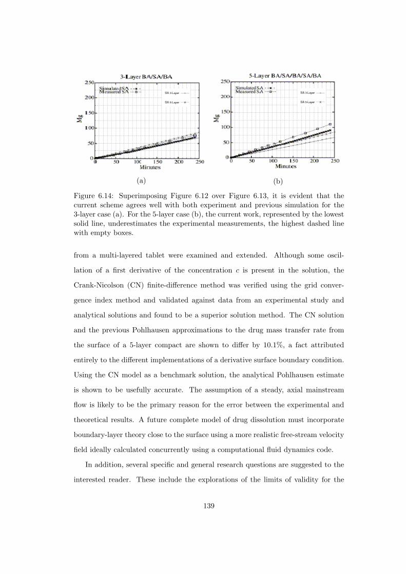
(a) (b)

Figure 6.14: Superimposing Figure 6.12 over Figure 6.13, it is evident that thecurrent scheme agrees well with both experiment and previous simulation for the3-layer case (a). For the 5-layer case (b), the current work, represented by the lowestsolid line, underestimates the experimental measurements, the highest dashed linewith empty boxes.

from a multi-layered tablet were examined and extended. Although some oscil-

lation of a first derivative of the concentration c is present in the solution, the

Crank-Nicolson (CN) finite-difference method was verified using the grid conver-

gence index method and validated against data from an experimental study and

analytical solutions and found to be a superior solution method. The CN solution

and the previous Pohlhausen approximations to the drug mass transfer rate from

the surface of a 5-layer compact are shown to differ by 10.1%, a fact attributed

entirely to the different implementations of a derivative surface boundary condition.

Using the CN model as a benchmark solution, the analytical Pohlhausen estimate

is shown to be usefully accurate. The assumption of a steady, axial mainstream

flow is likely to be the primary reason for the error between the experimental and

theoretical results. A future complete model of drug dissolution must incorporate

boundary-layer theory close to the surface using a more realistic free-stream velocity

field ideally calculated concurrently using a computational fluid dynamics code.

In addition, several specific and general research questions are suggested to the

interested reader. These include the explorations of the limits of validity for the

139

Pohlhausen solution, to further clarify the reasons for its deviation from the CN

solution and to formally demonstrate that its convergence as the number of layers

becomes very large can be written in a closed form. In addition, it will be interesting

to formulate other applications for the extended Pohlhausen solution. These may

have some utility when considering matrix tablets, where the drug is dispersed as

very small particles throughout the tablet, i.e. a large number of layers may ap-

proximate matrix tablet behaviour. Other applications may include microelectrode

analysis. The CN finite-difference method can be extended in many ways including

the already mentioned consideration of more realistic flows from a coupled CFD

code. There are many outstanding investigations around the CN scheme, including,

e.g. detailed investigations of its validity and incorporation of more efficient mesh

distributions.

Importantly, this study demonstrates that simulation, which includes mathe-

matical and numerical approaches, is useful in the description of pharmaceutical

processes. Chapter 7 continues with results from the second of the three studies

that contribute to this thesis.

140

φ = m 1-Layer Results 3-Layer Results 5-Layer Results

[BA] [-/BA/-] [-/BA/-/BA/-]

N1, N2, N3 40000, 10000, 2500 40000, 10000, 2500 40000, 10000, 2500

h1, h2, h3 0.0002, 0.0005, 0.002 0.0002, 0.0005, 0.002 0.0002, 0.0005, 0.002

r21 2.25 2.25 2.25

r32 4 4 4

φ1 1.129213644 0.504887462 0.638030816

φ2 1.129316609 0.504879397 0.637924898

φ3 1.129940559 0.50451875 0.637449681

ǫ21 0.000102965 -8.06485E-06 -0.000105918

ǫ32 0.00062395 -0.000360647 -0.000475217

p 1.095741391 2.67159063 0.844602624

φ21ext 1.129141723 0.504888506 0.638138499

φ32ext 1.129141723 0.504888506 0.638138499

ǫ21a 0.01% 0.0016% 0.02%

ǫ21ext 0.01% 0.0002% 0.02%

GCI21fine 0.01% 0.0003% 0.02%

Table 6.3: Calculating the grid convergence index for the Crank-Nicolson finitedifference scheme presented in this thesis. The procedure is the same as outlined byCelik [149].

141

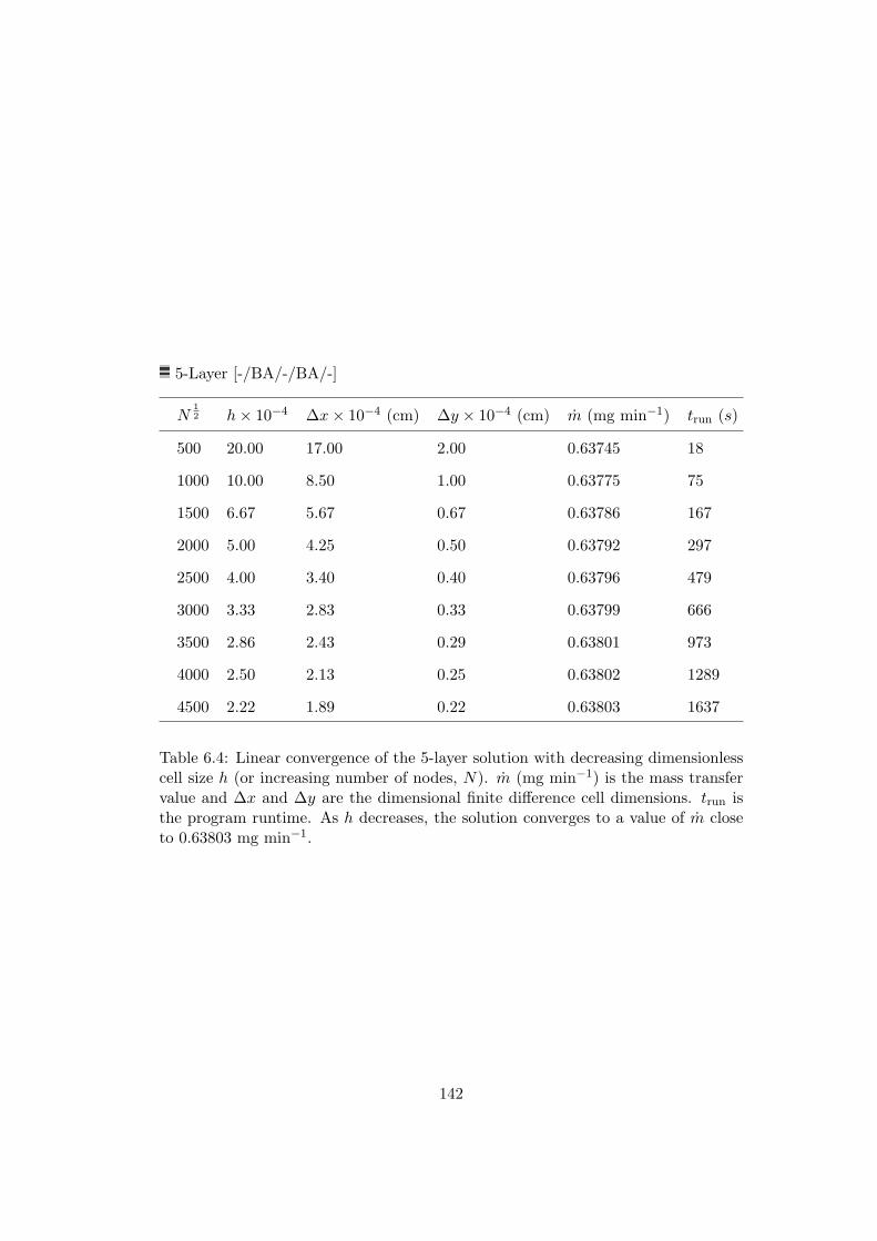
5-Layer [-/BA/-/BA/-]

N12 h× 10−4 ∆x× 10−4 (cm) ∆y × 10−4 (cm) m (mg min−1) trun (s)

500 20.00 17.00 2.00 0.63745 18

1000 10.00 8.50 1.00 0.63775 75

1500 6.67 5.67 0.67 0.63786 167

2000 5.00 4.25 0.50 0.63792 297

2500 4.00 3.40 0.40 0.63796 479

3000 3.33 2.83 0.33 0.63799 666

3500 2.86 2.43 0.29 0.63801 973

4000 2.50 2.13 0.25 0.63802 1289

4500 2.22 1.89 0.22 0.63803 1637

Table 6.4: Linear convergence of the 5-layer solution with decreasing dimensionlesscell size h (or increasing number of nodes, N). m (mg min−1) is the mass transfervalue and ∆x and ∆y are the dimensional finite difference cell dimensions. trun isthe program runtime. As h decreases, the solution converges to a value of m closeto 0.63803 mg min−1.

142

Data Source 1-Layer 3-Layer 5-Layer

[BA] [-/BA/-] [-/BA/-/BA/-]

Experiment

Healy et al. [104] 1.46 (-) 0.64 (-) 0.73 (-)

(Semi-)Analytical Models

Crane et al. [17] 1.17 (19.8) - -

Kestin and Persen [108] 1.13 (22.9) 0.51 (21.6) -

Pohlhausen [21] 1.13 (23.0) 0.51 (21.6) 0.58 (20.9)


McMahon et al. [261] 1.13 (22.9) 0.51 (21.6) 0.64 (12.9)

Table 6.5: Experimental and theoretical values for the mass transfer rate of benzoicacid (BA) from 1/3/5-Layer compacts dissolving in a USP dissolution apparatus,m (mg min−1). Percentage errors with respect to the experimental values are listedin brackets (%). The experimental values for 3/5 layer compacts are inferred fromfigures for salicylic acid in [21].

143

Data Source 1-Layer 3-Layer 5-Layer

[BA] [-/BA/-] [-/BA/-/BA/-]

Experiment

Healy et al. [104] 1.00 (29.8) 0.44 (27.5) 0.50 (26.4)

(Semi-)Analytical Models

Crane et al. [17] 1.00 (4.1) - -

Kestin and Persen [108] 1.00 (0.1) 0.45 (0.1) -

Pohlhausen [21] 1.00 (-) 0.45 (-) 0.51 (-)


McMahon et al. [261] 1.00 (0.1) 0.45 (0.1) 0.57 (10.1)

Table 6.6: Experimental and theoretical values for the mass transfer rate of benzoicacid (BA) normalised with respect to 1-layer values. Percentage difference of masstransfer rates with respect to the Pohlhausen values are listed in brackets (%). The10.1% discrepancy between the Pohlhausen and finite difference methods resultsfrom the different implementations of the Neumann boundary condition only. Animportant point is that although the finite difference results is a little further fromthe reported experimental value, the reasons why this is so are quite well understood.

144

Chapter 7


In this chapter we present results from the second of two studies presented in this

thesis, the flow around the top of a cylinder. The significance of these results, as

well as their context in the overall thesis, is discussed.

7.1 2D Validation with Comparisons of Flow Around a

Circular Cylinder

7.1.1 Qualitative 2D Validation

Visual comparisons of the flow patterns around a circular cylinder predicted by

Fluent and experimental visualisations and descriptions in the literature formed part

of our validation. The classification and description of the flow regimes discussed are

taken from Coutanceau and Defaye’s 1991 review paper [212]. This complete paper

contains many striking images of two dimensional flow about circular cylinders and

a flow regime classification with careful description.

The first flow regime considered consisted of flows of Reynolds number (Re)

between 35 and 60 [212] . In this range, flow instabilities appear, with slight asym-

metry of the attached wake bubble and less well defined boundaries between the

wake bubble and the surrounding, increasingly wavy, wake flow. For a laminar

145

(a) (b)

Figure 7.1: (a) Flow pattern around an infinite, or 2D, cylinder with Re = 50. (b)Flow around the same cylinder but with Re = 80. These images were generatedusing the commercial CFD code Fluent as a demonstration and validation of itscapabilities. The flow patterns agree well with experimental observations [212].

incident flow at a Reynolds number of 50, the flow pattern generated by Fluent

compares favourably with experimental description (Figure 7.1 (a)).

The second flow regime considered consists of flows where 60 < Re < 100. In

this range the wake asymmetries are pronounced, leading to vortex shedding from

alternate sides of the cylinder [212]1. The output from Fluent for a laminar incident

flow again agrees well with experiment (Figure 7.1 (b)). The attached bubble can

be seen on the bottom right of the cylinder with a shed vortex downstream.

The final flow regime considered as part of this visual comparison with exper-

iment is defined by flows where 2 × 103 < Re < 100 × 103. Flows in this regime

still display a laminar boundary-layer which separates from the surface at about 80

from the stagnation point at the front of the cylinder; this separation point moves

forward as the Reynolds number increases [212]. An irregular secondary boundary-

layer is formed and a turbulent von Karman vortex street is fully established. As

illustrated in Figure 7.2, the Fluent solution for a flow of Re = 3900 agrees well

with this description and with experimental visualisations [e.g. 263; 212].

1The asymmetric vortices are caused by small oscillations in the pressure distribution aroundthe cylinder.

146

(a) (b)

Figure 7.2: (a) Fluent generated 2D flow around an infinite cylinder with Re =3, 900. (b) An experimental visualisation of 2D flow at a Re = 2, 000, taken from[263]. These systems fall within flow Regime 7, 2, 000 < Re < 100, 000 [212]. TheFluent solution agrees well with this observed flow.

7.1.2 Quantitative 2D Validation

Our quantitative validations focused on measurable quantities such as the drag coef-

ficient, Cd, the circumferential pressure coefficient Cp and the angle of separation, θ.

For laminar flow regimes, up to Re ≈ 103 [212], the Fluent estimates for Cd compare

well with classic experimental studies [e.g 210; 213] (Figure 7.3 and Table 7.1). The

Fluent generated output agrees well with experimental results for Cd, Cp and θ from

several large eddy simulation models as well as the experimental measurements for

Re = 3, 900 presented by Franke et al. [206] (see Table 7.2).

It is evident however, that reasonably well is the strongest statement that can

possibly be made about how well the Fluent data matches results from other studies.

There is ample room for disagreement about this positive assessment. The results

for the flow variables are extremely sensitive to boundary conditions, small changes

in the cylinder geometry, and small disturbances in the calculated flow caused by

numerical error, e.g. truncation and rounding errors [206]. Variables evaluated

close to the surface of the cylinder can be particularly sensitive to grid resolution.

Experimental studies are extremely sensitive to test rig variables, including the

aspect ratio of the test channel, blockage effects, end conditions and the turbulence

intensity of the flow. It is important to bear all this in mind when comparing results

for apparently similar systems. It is reasonable, given that the Fluent simulation

produces qualitatively correct results especially away from the surface, to state that

147

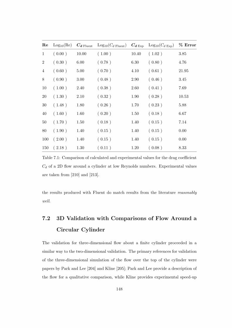
Re Log10(Re) Cd Fluent Log10(Cd Fluent) Cd Exp Log10(Cd Exp) % Error

1 ( 0.00 ) 10.00 ( 1.00 ) 10.40 ( 1.02 ) 3.85

2 ( 0.30 ) 6.00 ( 0.78 ) 6.30 ( 0.80 ) 4.76

4 ( 0.60 ) 5.00 ( 0.70 ) 4.10 ( 0.61 ) 21.95

8 ( 0.90 ) 3.00 ( 0.48 ) 2.90 ( 0.46 ) 3.45

10 ( 1.00 ) 2.40 ( 0.38 ) 2.60 ( 0.41 ) 7.69

20 ( 1.30 ) 2.10 ( 0.32 ) 1.90 ( 0.28 ) 10.53

30 ( 1.48 ) 1.80 ( 0.26 ) 1.70 ( 0.23 ) 5.88

40 ( 1.60 ) 1.60 ( 0.20 ) 1.50 ( 0.18 ) 6.67

50 ( 1.70 ) 1.50 ( 0.18 ) 1.40 ( 0.15 ) 7.14

80 ( 1.90 ) 1.40 ( 0.15 ) 1.40 ( 0.15 ) 0.00

100 ( 2.00 ) 1.40 ( 0.15 ) 1.40 ( 0.15 ) 0.00

150 ( 2.18 ) 1.30 ( 0.11 ) 1.20 ( 0.08 ) 8.33

Table 7.1: Comparison of calculated and experimental values for the drag coefficient

Cd of a 2D flow around a cylinder at low Reynolds numbers. Experimental values

are taken from [210] and [213].

the results produced with Fluent do match results from the literature reasonably

well.

7.2 3D Validation with Comparisons of Flow Around a

Circular Cylinder

The validation for three-dimensional flow about a finite cylinder proceeded in a

similar way to the two-dimensional validation. The primary references for validation

of the three-dimensional simulation of the flow over the top of the cylinder were

papers by Park and Lee [204] and Kline [205]; Park and Lee provide a description of

the flow for a qualitative comparison, while Kline provides experimental speed-up

148

0.0

0.2

0.4

0.6

0.8

1.0

1.2

1.4

1.6

1.8

2.0

-1.00 -0.50 0.00 0.50 1.00 1.50 2.00 2.50

Log

Cd

Log Re

Experimenta

Fluent

Figure 7.3: Comparison of calculated and experimental values for the drag coefficientCd of a 2D flow around a cylinder at low Reynolds numbers, ranging from 0.2 to150. Note: (a) these values are taken from [210] and [213].

measurements.

7.2.1 Qualitative 3D Validation

As illustrated in Figure 7.4, the visualised Fluent solution for a 3D flow of Reynolds

number 20,000 past a finite cylinder of height to diameter ratio 5 (H/D = 5) agrees

well with the experimental flow observed and recorded by Park and Lee [204]. This

is particularly true in the region of interest directly above the top of the cylinder.

7.2.2 Quantitative 3D Validation

Uematsu and Yamada [266; 218] present experimental data for flows around finite

cylinders with Re ≥ 38 × 103. Values for the drag coefficient (Cd) of the 3D finite

cylinder correspond with experimental values [218] (Cd ≈ 0.60, which falls within

the range of experimental measurements for a H/D = 3). The authors also present

results for the measured circumferential pressure coefficient (Cp) distribution around

the middle (H/2) of a finite cylinder with H/D = 3. These distributions are mea-

149

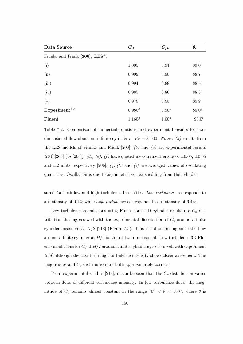
Data Source Cd Cpb θs

Franke and Frank [206], LESa:

(i) 1.005 0.94 89.0

(ii) 0.999 0.90 88.7

(iii) 0.994 0.88 88.5

(iv) 0.985 0.86 88.3

(v) 0.978 0.85 88.2

Experimentb,c 0.980d 0.90e 85.0f

Fluent 1.160g 1.00h 90.0i

Table 7.2: Comparison of numerical solutions and experimental results for two-

dimensional flow about an infinite cylinder at Re = 3, 900. Notes: (a) results from

the LES models of Franke and Frank [206]; (b) and (c) are experimental results

[264] [265] (in [206]); (d), (e), (f) have quoted measurement errors of ±0.05, ±0.05

and ±2 units respectively [206]; (g),(h) and (i) are averaged values of oscillating

quantities. Oscillation is due to asymmetric vortex shedding from the cylinder.

sured for both low and high turbulence intensities. Low turbulence corresponds to

an intensity of 0.1% while high turbulence corresponds to an intensity of 6.4%.

Low turbulence calculations using Fluent for a 2D cylinder result in a Cp dis-

tribution that agrees well with the experimental distribution of Cp around a finite

cylinder measured at H/2 [218] (Figure 7.5). This is not surprising since the flow

around a finite cylinder at H/2 is almost two-dimensional. Low turbulence 3D Flu-

ent calculations for Cp atH/2 around a finite cylinder agree less well with experiment

[218] although the case for a high turbulence intensity shows closer agreement. The

magnitudes and Cp distribution are both approximately correct.

From experimental studies [218], it can be seen that the Cp distribution varies

between flows of different turbulence intensity. In low turbulence flows, the mag-

nitude of Cp remains almost constant in the range 70 < θ < 180, where θ is

150

(a) (b)

Figure 7.4: (a) Fluent generated 3D flow around a finite cylinder of H/D = 5 atRe = 20, 000. (b) An experimental visualisation of 3D flow past a similar cylinderat Re = 20, 000. Reprinted from [204], Copyright (2000), with permission fromElsevier.

-2.4

-2.0

-1.6

-1.2

-0.8

-0.4

0.0

0.4

0.8

1.2

1.6

2.0

180o165o150o135o120o105o90o75o60o45o30o15o0o

Cp

Position

(i)

-2.4

-2.0

-1.6

-1.2

-0.8

-0.4

0.0

0.4

0.8

1.2

1.6

2.0

180o150o120o90o60o30o0o

Cp

Position

(ii)

Figure 7.5: (i) Cp at Re = 38×103 for 2D flow around a cylinder, (ii) Cp distributionat H/2 for low flow turbulence around a finite cylinder.

measured from the forward stagnation point. In the high turbulence case, however,

Cp does not begin to level off until at least θ ≈ 110.

Since Cp on the windward side of the cylinder agrees quite well with literature

and as we were interested, for this problem, in the flow several diameters vertically

above the cylinder, the flow on the lee-side of the cylinder will not have an effect

in this region. In the region of interest, one diameter above the cylinder, close wall

151

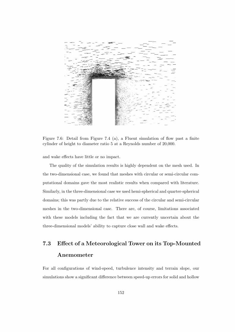
Figure 7.6: Detail from Figure 7.4 (a), a Fluent simulation of flow past a finitecylinder of height to diameter ratio 5 at a Reynolds number of 20,000.

and wake effects have little or no impact.

The quality of the simulation results is highly dependent on the mesh used. In

the two-dimensional case, we found that meshes with circular or semi-circular com-

putational domains gave the most realistic results when compared with literature.

Similarly, in the three-dimensional case we used hemi-spherical and quarter-spherical

domains; this was partly due to the relative success of the circular and semi-circular

meshes in the two-dimensional case. There are, of course, limitations associated

with these models including the fact that we are currently uncertain about the

three-dimensional models’ ability to capture close wall and wake effects.

7.3 Effect of a Meteorological Tower on its Top-Mounted

Anemometer

For all configurations of wind-speed, turbulence intensity and terrain slope, our

simulations show a significant difference between speed-up errors for solid and hollow

152

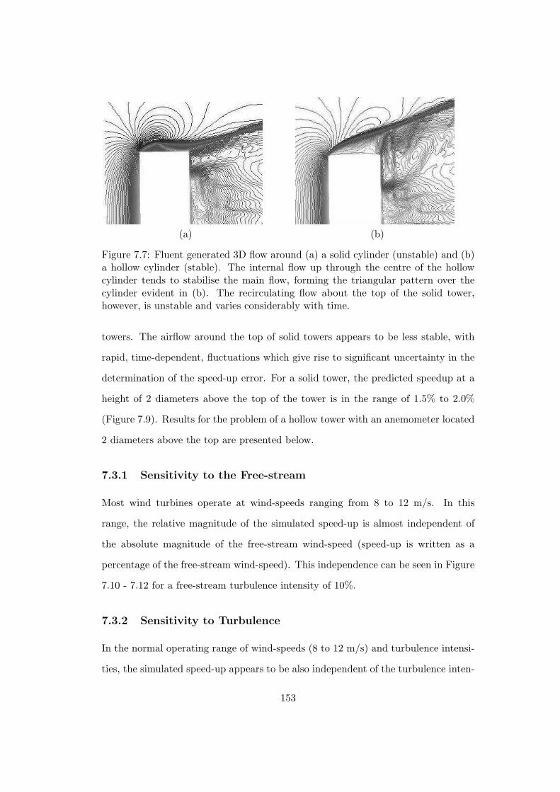
(a) (b)

Figure 7.7: Fluent generated 3D flow around (a) a solid cylinder (unstable) and (b)a hollow cylinder (stable). The internal flow up through the centre of the hollowcylinder tends to stabilise the main flow, forming the triangular pattern over thecylinder evident in (b). The recirculating flow about the top of the solid tower,however, is unstable and varies considerably with time.

towers. The airflow around the top of solid towers appears to be less stable, with

rapid, time-dependent, fluctuations which give rise to significant uncertainty in the

determination of the speed-up error. For a solid tower, the predicted speedup at a

height of 2 diameters above the top of the tower is in the range of 1.5% to 2.0%

(Figure 7.9). Results for the problem of a hollow tower with an anemometer located

2 diameters above the top are presented below.

7.3.1 Sensitivity to the Free-stream

Most wind turbines operate at wind-speeds ranging from 8 to 12 m/s. In this

range, the relative magnitude of the simulated speed-up is almost independent of

the absolute magnitude of the free-stream wind-speed (speed-up is written as a

percentage of the free-stream wind-speed). This independence can be seen in Figure

7.10 - 7.12 for a free-stream turbulence intensity of 10%.

7.3.2 Sensitivity to Turbulence

In the normal operating range of wind-speeds (8 to 12 m/s) and turbulence intensi-

ties, the simulated speed-up appears to be also independent of the turbulence inten-

153

Figure 7.8: Sample anemometer positions (in steps of 30) around the circumferenceof the meteorological tower. The wind blows from left to right. The anemometercups are located two diameters above the top of the tower.

sity of the free-stream (Figure 7.13). This conclusion is based on two simulation runs

with turbulence intensities of 10% and 15% and implies that the anemometer data

can be corrected without any complications arising from turbulence in the airflow.

Together with the previous observation (Section 7.3.1), we find that the speed-up

can be associated with a particular anemometer set-up and is dependent only on

quantities that can be determined (terrain slope, tower geometry, fluid properties

and tower surface conditions).

7.3.3 Sensitivity to Sloped Terrain

Airflow is accelerated when passing over a hill and, for this reason, wind farms are

often sited on slopes. For practical considerations, these slopes never exceed 25.

Simulation runs at slopes of 0, 15 and 25 indicated that, as expected, the speed-

up has a significant dependence on terrain slope (Figure 7.14 and 7.15). However,

154

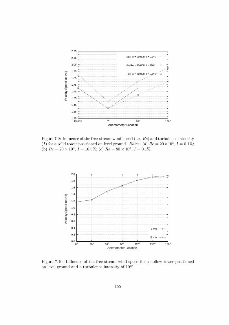
1.25

1.35

1.45

1.55

1.65

1.75

1.85

1.95

2.05

2.15

2.25

Centre 0o 90o 180o

Velo

city S

peed-u

p (

%)

Anemometer Location

(a) Re = 20,000, I = 0.1%

(b) Re = 20,000, I = 10%

(c) Re = 80,000, I = 0.1%

Figure 7.9: Influence of the free-stream wind-speed (i.e. Re) and turbulence intensity(I) for a solid tower positioned on level ground. Notes: (a) Re = 20×103, I = 0.1%;(b) Re = 20 × 103, I = 10.0%; (c) Re = 80 × 103, I = 0.1%.

0.0

0.2

0.4

0.6

0.8

1.0

1.2

1.4

1.6

1.8

2.0

0o 30o 60o 90o 120o 150o 180o

Vel

ocity

Spe

ed-u

p (%

)

Anemometer Location

8 m/s

12 m/s

Figure 7.10: Influence of the free-stream wind-speed for a hollow tower positionedon level ground and a turbulence intensity of 10%.

155

0.0

0.2

0.4

0.6

0.8

1.0

1.2

1.4

1.6

1.8

2.0

0o 30o 60o 90o 120o 150o 180o

Vel

ocity

Spe

ed-u

p (%

)

Anemometer Location

8 m/s

12 m/s

Figure 7.11: Influence of the free-stream wind-speed for a hollow tower positionedon a slope of 15 and a turbulence intensity of 10%.

0.0

0.2

0.4

0.6

0.8

1.0

1.2

1.4

1.6

1.8

2.0

0o 30o 60o 90o 120o 150o 180o

Vel

ocity

Spe

ed-u

p (%

)

Anemometer Location

8 m/s

12 m/s

Figure 7.12: Influence of the free-stream wind-speed for a hollow tower positionedon a slope of 25 and a turbulence intensity of 10%.

156

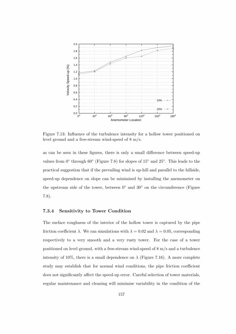
0.0

0.2

0.4

0.6

0.8

1.0

1.2

1.4

1.6

1.8

2.0

0o 30o 60o 90o 120o 150o 180o

Vel

ocity

Spe

ed-u

p (%

)

Anemometer Location

10%

15%

Figure 7.13: Influence of the turbulence intensity for a hollow tower positioned onlevel ground and a free-stream wind-speed of 8 m/s.

as can be seen in these figures, there is only a small difference between speed-up

values from 0 through 60 (Figure 7.8) for slopes of 15 and 25. This leads to the

practical suggestion that if the prevailing wind is up-hill and parallel to the hillside,

speed-up dependence on slope can be minimised by installing the anemometer on

the upstream side of the tower, between 0 and 30 on the circumference (Figure

7.8).

7.3.4 Sensitivity to Tower Condition

The surface roughness of the interior of the hollow tower is captured by the pipe

friction coefficient λ. We ran simulations with λ = 0.02 and λ = 0.05, corresponding

respectively to a very smooth and a very rusty tower. For the case of a tower

positioned on level ground, with a free-stream wind-speed of 8 m/s and a turbulence

intensity of 10%, there is a small dependence on λ (Figure 7.16). A more complete

study may establish that for normal wind conditions, the pipe friction coefficient

does not significantly affect the speed-up error. Careful selection of tower materials,

regular maintenance and cleaning will minimise variability in the condition of the

157

0.0

0.2

0.4

0.6

0.8

1.0

1.2

1.4

1.6

1.8

2.0

0o 30o 60o 90o 120o 150o 180o

Vel

ocity

Spe

ed-u

p (%

)

Anemometer Location

No slope

15o slope

25o slope

Figure 7.14: Influence of terrain slope for a hollow tower in a free-stream wind-speedof 8 m/s and a turbulence intensity of 10%.

0.0

0.2

0.4

0.6

0.8

1.0

1.2

1.4

1.6

1.8

2.0

0o 30o 60o 90o 120o 150o 180o

Vel

ocity

Spe

ed-u

p (%

)

Anemometer Location

No slope

15o slope

25o slope

Figure 7.15: Influence of terrain slope for a hollow tower in a free-stream wind-speedof 12 m/s and a turbulence intensity of 10%.

158

0.0

0.2

0.4

0.6

0.8

1.0

1.2

1.4

1.6

1.8

2.0

0o 30o 60o 90o 120o 150o 180o

Vel

ocity

Spe

ed-u

p (%

)

Anemometer Location

λ = 0.02

λ = 0.05

Figure 7.16: Influence of the pipe friction coefficient λ for a hollow tower positionedon level ground, a free-stream wind-speed of 8 m/s and a turbulence intensity of10%.

tower and of any effect that the surface roughness (and debris) will have on the

airflow through and around the structure.

7.3.5 Speed-up Envelope

In addition to the speed-up values for anemometers located 2 diameters above the

top of the tower, we also recorded wind-speed values at various heights above the

centre of the tower. The speed-up decreases as the distance above the tower in-

creases. This is shown in Figure 7.17 for a wind-speed of 12 m/s and a turbulence

intensity of 10%. Engineers and technicians may find this plot useful when locating

anemometers.


In summary, this chapter presented results from the second of three studies described

in this thesis.

159

0.0

0.5

1.0

1.5

2.0

2.5

3.0

3.5

1.0 1.5 2.0 2.5 3.0 3.5 4.0 4.5 5.0

Vel

ocity

Spe

ed-u

p (%

)

Height above tower (in diameters)

No slope

15o slope

25o slope

Figure 7.17: Speed-up values at various heights above the centre of a hollow towerpositioned on level ground.

This second study began with an investigation of the flow around a finite cylinder

with attention given to the problem of determining the measurement error due to

speed-up for the specific case of an anemometer located 2 diameters above the

top of a hollow meteorological tower sited on level terrain. It was found that the

maximum error for this configuration is approximately 2% of the actual wind-speed

(Figure 7.10). This compares well with experimental measurements for a hollow

meteorological tower, which range from 1.7% to 3.4% [205].

It is concluded that the speed-up over the top of a hollow meteorological tower

depends only on variables that can be determined. Speed-up is independent of the

absolute magnitude of the free-stream wind-speed and the turbulence intensity of

the wind. The error depends on the geometry of the meteorological tower, the slope

of the terrain where the tower is sited and the condition of the tower.

In summary, top-mounted anemometers should be located at the windward side

of a meteorological tower, where a particular wind direction prevails, and at least

5 diameters above the top. This will reduce speed-up to less that 1%. The IEA

recommendation is for a minimum separation of about 6 tower diameters [203].

160

In line with the IEA’s recommendation that the anemometer installation should

be ‘clean’ [203], towers should be made from a corrosion resistant material and

maintained and cleaned regularly to minimise flow disturbance.

Many other research problems are indicated; in the area of wind energy, several

new refinements of the work developed here are essential and will make a useful

contribution to the field. These include extending the analysis for different tower

and anemometer configurations and for different tower types, e.g. considering the

error in wind-speed measurements from anemometers mounted close to the side of

a meteorological tower. Another useful study will be to further refine the simple

turbulence model used and to carry out a more complete study of the effect of

turbulence.

Although not pursued explicitly, techniques developed here for the problem of

flow around a meteorological tower can be applied to the similar problem of flow

around a finite cylindrical tablet. Using the specific problem outlined here as a basis,

it is argued that simulation can provide useful insight for similar pharmaceutical

problems. Chapter 8 continues with results from the third of the three studies that

contribute to this thesis.

161

Chapter 8


In this chapter we present results from the final of the three primary investigations

presented in this thesis, mass transfer from a particle moving through the USP

apparatus. The significance of these results, as well as their context in the overall

thesis, is discussed. Unless specified otherwise, the equations of motion used to

produce the results presented in this chapter were Equations (5.4 - 5.9).

8.1 Computer Implementation of Taylor’s Work

Results for two different initial conditions were calculated, (1) with the particle

assumed to be at rest with respect to the reference frame at t = 0 and (2) with

the particle assumed to move with the flow at t = 0. In addition, solutions were

calculated when (i) Stokes’ law of resistance applies, using Equations (5.11) and

(5.12) and (ii) Stokes’ law does not apply, using Equations (5.13) and (5.14). A

sample of these results is presented in Table 8.1.

Figure 8.1 (a) is a plot of the particle path for α = K0c = 0.5, all defined

previously, with Stokes’ law of resistance assumed to apply and with the particle

initially at rest1. Figure 8.1 (b) shows the particle path for the same α when Stokes’

law does not apply, the particle is moving with the flow at t = 0 and the initial

1As discussed in Chapter 5, α is a parameter which is a function of a2c.

162

0.0

0.5

1.0

1.5

2.0

2.5

3.0

3.5

4.0

4.5

5.0

5.5

6.0

6.5

7.0

0.00.10.20.30.40.50.60.70.80.91.00.0

0.5

1.0

1.5

2.0

2.5

3.0

3.5

4.0

4.5

5.0

5.5

6.0

6.5

7.0y/

Y

x/X

Calculated Paths of Drops and Streamlines near a Stagnation Point

Stokes Flow

Stream lines

Stagnation point

(a)

0.0

0.5

1.0

1.5

2.0

2.5

3.0

3.5

4.0

4.5

5.0

5.5

6.0

6.5

7.0

0.00.10.20.30.40.50.60.70.80.91.00.0

0.5

1.0

1.5

2.0

2.5

3.0

3.5

4.0

4.5

5.0

5.5

6.0

6.5

7.0

y/Y

x/X


Stokes Flow

Stream lines

Stagnation point

(c)

0.0

0.5

1.0

1.5

2.0

2.5

3.0

3.5

4.0

4.5

5.0

5.5

6.0

6.5

7.0

0.00.10.20.30.40.50.60.70.80.91.00.0

0.5

1.0

1.5

2.0

2.5

3.0

3.5

4.0

4.5

5.0

5.5

6.0

6.5

7.0

y/Y

x/X


Fully variable Drag Coefficient, Cd

Stream lines

Stagnation point

(b)

(d)

Figure 8.1: (a): α = 0.5, Stokes flow, particle initially at rest. (b) α = 0.5, Stokes’law does not apply, particle initially moving with the flow. (c): α = 0.5, Stokes’flow, particle initially moving with flow. (d) Reproduced from Taylor’s paper [22]:α = 0.5, Stokes’ flow, particle initially moving with flow.

163

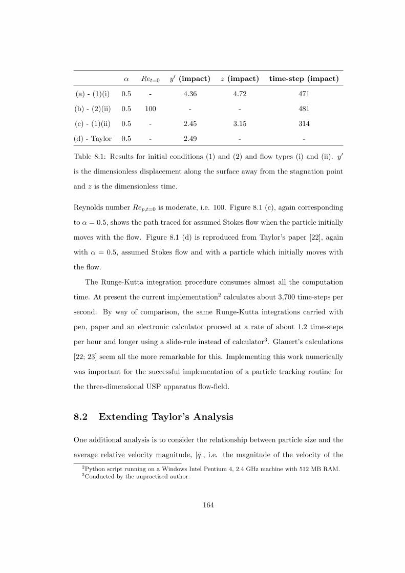
α Ret=0 y′ (impact) z (impact) time-step (impact)

(a) - (1)(i) 0.5 - 4.36 4.72 471

(b) - (2)(ii) 0.5 100 - - 481

(c) - (1)(ii) 0.5 - 2.45 3.15 314

(d) - Taylor 0.5 - 2.49 - -

Table 8.1: Results for initial conditions (1) and (2) and flow types (i) and (ii). y′

is the dimensionless displacement along the surface away from the stagnation point

and z is the dimensionless time.

Reynolds number Rep,t=0 is moderate, i.e. 100. Figure 8.1 (c), again corresponding

to α = 0.5, shows the path traced for assumed Stokes flow when the particle initially

moves with the flow. Figure 8.1 (d) is reproduced from Taylor’s paper [22], again

with α = 0.5, assumed Stokes flow and with a particle which initially moves with

the flow.

The Runge-Kutta integration procedure consumes almost all the computation

time. At present the current implementation2 calculates about 3,700 time-steps per

second. By way of comparison, the same Runge-Kutta integrations carried with

pen, paper and an electronic calculator proceed at a rate of about 1.2 time-steps

per hour and longer using a slide-rule instead of calculator3. Glauert’s calculations

[22; 23] seem all the more remarkable for this. Implementing this work numerically

was important for the successful implementation of a particle tracking routine for

the three-dimensional USP apparatus flow-field.

8.2 Extending Taylor’s Analysis

One additional analysis is to consider the relationship between particle size and the

average relative velocity magnitude, |q|, i.e. the magnitude of the velocity of the

2Python script running on a Windows Intel Pentium 4, 2.4 GHz machine with 512 MB RAM.3Conducted by the unpractised author.

164

particle with respect to the fluid, averaged over a fixed simulation time, ts. It is

speculated that |q| will increase with particle size, defined by particle radius a, and

approach a limit as the particle size becomes large. Taking the case when Stokes’

law applies, i.e. for very low average relative Reynolds numbers Rep between the

particle and the fluid, Taylor’s problem of a particle moving close to a stagnation

point can be solved using primitive variables with Equations (5.4 and 5.5).

Solving these equations using the Euler/LPA algorithm, the particle position and

velocity components u and v as well as the resultant velocity q at each timestep in

the interval t = 0 to t = ts were determined. The relative velocity magnitude |q| was

then calculated at each timestep and averaged over the simulated time ts. Results for

particles of various sizes moving through a stagnation flow, i.e. u = −cx and v = cy,

with velocities defined by c = 0.5 are presented in Table 8.2. The calculations were

run for a simulated time of ts for all the particle sizes. The resulting average relative

velocity |q| averaged over ts for each a is graphed in Figure 8.2.

a (mm) c ∆t (s) |qp| cm s−1 |qf | cm s−1 |q| Rep

0.100 0.500 0.004 0.817 0.863 0.046 0.291

0.200 0.500 0.004 0.641 0.756 0.115 1.452

0.300 0.500 0.004 0.536 0.685 0.148 2.800

0.400 0.500 0.004 0.496 0.645 0.150 3.767

0.500 0.500 0.004 0.484 0.623 0.139 4.379

0.600 0.500 0.004 0.482 0.609 0.127 4.809

0.700 0.500 0.004 0.483 0.601 0.117 5.168

0.800 0.500 0.004 0.485 0.595 0.109 5.507

0.900 0.500 0.004 0.487 0.591 0.103 5.848

1.000 0.500 0.004 0.489 0.588 0.098 6.198

Table 8.2: Calculated quantities for various particles of various diameter a movingthrough the stagnation flow described by Taylor [22]. |qp| and |qf | are the averageabsolute particle and fluid velocity magnitudes respectively.

165

0.00

0.02

0.04

0.06

0.08

0.10

0.12

0.14

0.16

0.18

0.20

0.1 0.2 0.3 0.4 0.5 0.6 0.7 0.8 0.9 1.0

Ave

rage

Rel

ativ

e V

eloc

ity (

m/s

)

Particle Radius (mm)

Figure 8.2: The average velocity relative to the fluid for particles of various diameter2a moving through the stagnation flow described by Taylor [22].

It is important to bear in mind that (i) the relatively inaccurate LPA/Euler ap-

proximation was used, (ii) Stokes flow is assumed, (iii) the particle size a is coupled

through an inverse proportionality to the freestream velocity. Velocities are calcu-

lated for a fixed simulated time ts, so that average velocities for a particular input

mainstream velocity can be compared.

Acknowledging these limitations, it can be seen that |q| initially increases with

increasing particle radius a before decreasing slightly to a fixed value as a becomes

large. This can be explained qualitatively as follows. Very light particles (e.g.

a = 0.01 cm) move almost entirely with the fluid streamlines and so |q| is very

small. As a grows larger, the particle begins to deviate from the fluid and cuts

streamlines in areas of relatively high velocity gradients. As a continues to grow,

the paths followed by successive particles become very similar (essentially straight

lines) and cut the fluid streamlines in areas of relatively low velocity gradient, i.e.

the relative velocity will be lower for larger particles. Small and light particles travel

with the flow while large and heavy particles move bullet-like through the flow with

very little deflection.

166

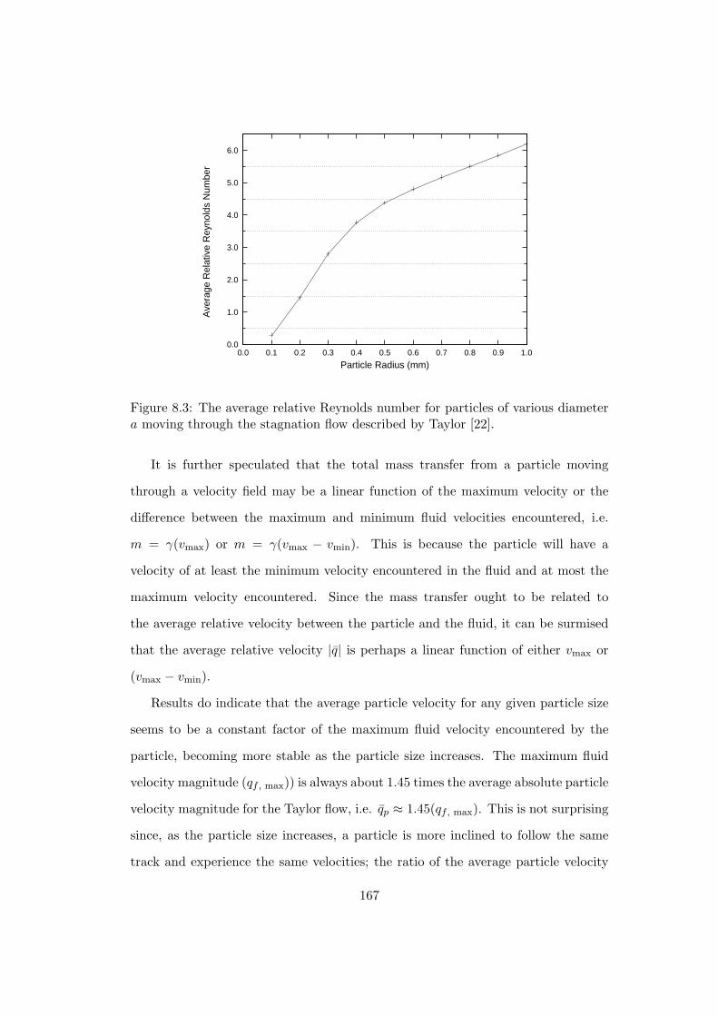
0.0

1.0

2.0

3.0

4.0

5.0

6.0

0.0 0.1 0.2 0.3 0.4 0.5 0.6 0.7 0.8 0.9 1.0

Ave

rage

Rel

ativ

e R

eyno

lds

Num

ber


Figure 8.3: The average relative Reynolds number for particles of various diametera moving through the stagnation flow described by Taylor [22].

It is further speculated that the total mass transfer from a particle moving

through a velocity field may be a linear function of the maximum velocity or the

difference between the maximum and minimum fluid velocities encountered, i.e.

m = γ(vmax) or m = γ(vmax − vmin). This is because the particle will have a

velocity of at least the minimum velocity encountered in the fluid and at most the

maximum velocity encountered. Since the mass transfer ought to be related to

the average relative velocity between the particle and the fluid, it can be surmised

that the average relative velocity |q| is perhaps a linear function of either vmax or

(vmax − vmin).

Results do indicate that the average particle velocity for any given particle size

seems to be a constant factor of the maximum fluid velocity encountered by the

particle, becoming more stable as the particle size increases. The maximum fluid

velocity magnitude (qf , max)) is always about 1.45 times the average absolute particle

velocity magnitude for the Taylor flow, i.e. qp ≈ 1.45(qf , max). This is not surprising

since, as the particle size increases, a particle is more inclined to follow the same

track and experience the same velocities; the ratio of the average particle velocity

167

and the maximum fluid velocity encountered by the particle should approach a

constant. It seems that a similar curve should exist for all velocity fields.

8.2.1 Particle Size and Average Relative Reynolds Number, Rep

For very small particles, fluid and particle motion will be practically identical at

each point in space, growing less similar with particle size until some critical value

when the particle never moves very closely with the fluid. For small particles which

move with the fluid, diffusion models, analytical and semi-analytical, are sufficient

to estimate the mass transfer and the particle motion simulation ends at this point.

There is no need for further calculation of the forced convective component of mass

transfer.

The most important relationship is that between the size of the particle, as

defined by its radius a, and the average relative Reynolds number (Rep) encountered.

The two-dimensional information considered was produced, as described in Section

5.4.

These results indicate that this mechanism is extant; there is a threshold or criti-

cal a below which convective mass transfer can be ignored and an analytical diffusion

mass transfer model applied. Extrapolating linearly from the two-dimensional plot

in Figure 8.5, we can say that for particles of diameter less than 0.05 mm, or 50

microns, the relative Reynolds number is practically zero and so we posit that an

analytical diffusion model can be be used for all particles of diameter 50 microns

and less.

8.3 USP Dissolution Apparatus

8.3.1 Particle Size and Average Reynolds Number

Following from the two-dimensional case, a plot of a against Rep for the three

dimensional flow in a USP apparatus should produce a curve with Rep high for

168

-0.06-0.04

-0.02 0

0.02 0.04

0.06-0.06

-0.04

-0.02

0

0.02

0.04

0.06

0

0.01

0.02

0.03

0.04

0.05

0.06

0.07

0.08

Figure 8.4: The streakline of a particle moving through the USP apparatus. Repre-senting a 100 second run, this path was generated using the CGNS data provided byDeirdre D’Arcy at the School of Pharmacy in Trinity College Dublin [19]. Visualisedfor this thesis using GnuPlot.

large a and tending to zero as a tends to zero. And indeed, this behaviour can be

clearly seen in Table 8.3 and Figure 8.5. Particle trajectories were calculated using

a simple LPA/Euler integration scheme and a nearest-neighbour search algorithm.

Particles are, however, not forced to the nearest node point after each time-step.

For particle diameters of 0.01 cm and smaller, the average relative Reynolds

number is very small, less than 0.04, see Table 8.3; the average relative Reynolds

number becomes small very quickly as the particle diameter decreases. This pattern

is seen for both the two-dimensional stagnation flow and the three dimensional USP

apparatus flow, shown in the diagram below.

169

a (cm) Rep

(i) (ii)

0.01 0.291 0.036

0.03 2.800 0.815

0.05 4.379 3.254

0.07 5.168 7.595

0.09 5.848 13.496

Table 8.3: Particle sizes with corresponding average Reynolds number relative tothe flow for (i) two-dimensional particle motion through a stagnation flow and (ii)particle motion through the three-dimensional velocity field with a USP apparatus(from data produced by Deirdre D’Arcy and others at the School of Pharmacy inTrinity College Dublin [19]).

0.0

2.0

4.0

6.0

8.0

10.0

12.0

14.0

0.0 0.1 0.2 0.3 0.4 0.5 0.6 0.7 0.8 0.9 1.0

Ave

rage

Rel

ativ

e R

eyno

lds

Num

ber


Figure 8.5: Particle sizes with corresponding average Reynolds number relative tothe flow for (i) two dimensional particle motion through a stagnation flow and (ii)particle motion through the three dimensional velocity field with a USP apparatus(from data produced by Deirdre D’Arcy and others at the School of Pharmacy inTrinity College Dublin [19]). Note that the particle radii are given in mm.

170

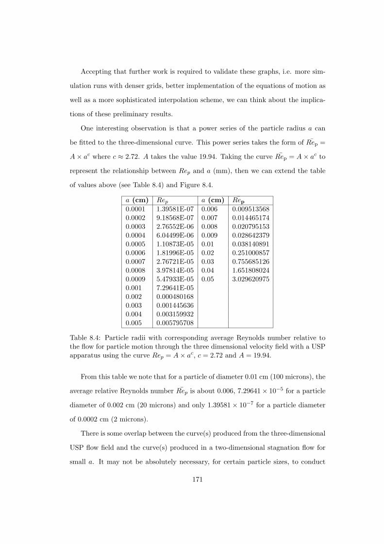
Accepting that further work is required to validate these graphs, i.e. more sim-

ulation runs with denser grids, better implementation of the equations of motion as

well as a more sophisticated interpolation scheme, we can think about the implica-

tions of these preliminary results.

One interesting observation is that a power series of the particle radius a can

be fitted to the three-dimensional curve. This power series takes the form of Rep =

A× ac where c ≈ 2.72. A takes the value 19.94. Taking the curve Rep = A× ac to

represent the relationship between Rep and a (mm), then we can extend the table

of values above (see Table 8.4) and Figure 8.4.

a (cm) Rep a (cm) Rep0.0001 1.39581E-07 0.006 0.0095135680.0002 9.18568E-07 0.007 0.0144651740.0003 2.76552E-06 0.008 0.0207951530.0004 6.04499E-06 0.009 0.0286423790.0005 1.10873E-05 0.01 0.0381408910.0006 1.81996E-05 0.02 0.2510008570.0007 2.76721E-05 0.03 0.7556851260.0008 3.97814E-05 0.04 1.6518080240.0009 5.47933E-05 0.05 3.0296209750.001 7.29641E-050.002 0.0004801680.003 0.0014456360.004 0.0031599320.005 0.005795708

Table 8.4: Particle radii with corresponding average Reynolds number relative tothe flow for particle motion through the three dimensional velocity field with a USPapparatus using the curve Rep = A× ac, c = 2.72 and A = 19.94.

From this table we note that for a particle of diameter 0.01 cm (100 microns), the

average relative Reynolds number Rep is about 0.006, 7.29641 × 10−5 for a particle

diameter of 0.002 cm (20 microns) and only 1.39581 × 10−7 for a particle diameter

of 0.0002 cm (2 microns).

There is some overlap between the curve(s) produced from the three-dimensional

USP flow field and the curve(s) produced in a two-dimensional stagnation flow for

small a. It may not be absolutely necessary, for certain particle sizes, to conduct

171

0.0

2.0

4.0

6.0

8.0

10.0

12.0

14.0

16.0

18.0

20.0

0.0 0.1 0.2 0.3 0.4 0.5 0.6 0.7 0.8 0.9 1.0

Ave

rage

Rel

ativ

e R

eyno

lds

Num

ber


Figure 8.6: Particle sizes with corresponding average Reynolds number relative tothe flow for particle motion through the three dimensional velocity field with a USPapparatus using the curve Rep = A × ac, c = 2.72 and A = 19.94. Note that theparticle radii are given in mm.

three-dimensional simulations; a single curve may suffice to describe the relationship

between a and Rep in all flows.

The mass transfer rate can be calculated piece-wise after each time-step ∆t using

an experimental correlation. In addition, when the relative Reynolds number is very

low, there is no need to calculate its motion through the fluid and a radial diffusion

model can be used.

8.3.2 Mass Transfer from a Particle in the USP Apparatus

Average mass transfer rates were calculated for particles of various diameters us-

ing experimental correlations, together with the quantities presented in Table 8.5

[254; 255; 256; 257]. Forced convective results were generated using the average

relative Reynolds numbers, presented in Section 8.3.1. Important dimensionless

172

0.00

0.50

1.00

1.50

2.00

2.50

3.00

3.50

4.00

0.0 0.1 0.2 0.3 0.4 0.5 0.6 0.7 0.8 0.9 1.0

Mas

s T

rans

fer

Rat

e (m

g/m

in)

Particle Diameter, 2a (cm)

Garner (Natural)

Garner (Forced)

Miller (Diffusion)

Miller (Natural)

Miller (Forced)

Figure 8.7: Average mass transfer rates for particles of various diameters usingexperimental correlations and the quantities presented in Table 8.5 [254; 255; 256;257]. Forced convective results were generated using the average relative Reynoldsnumbers presented in the Section 8.3.1. Garner’s natural convection model andMiller’s diffusion model converge to the same values for small particle sizes and aresuperimposed in this figure.

groups include the Reynolds number (Rep), Schmidt number (Sc), Grashof number

(G′ =8ga3

ν2

∆ρ

ρ) and the average Sherwood number, Shp =

2ahm

DAB. Results are

presented in Figures 8.7, 8.8 and 8.9.

Quantity Value

ρ (HCl) 1.186 g cm−3

ν (HCl) 7.870 × 10−3 cm2 s−1

Cs (Benzoic Acid) 4.550 × 10−3 g cm−3

∆ρ (Benzoic Acid in HCl) 1.990 × 10−3 g cm−3 [258]D (Benzoic Acid in HCl) 1.236 × 10−5 cm2 s−1

g 980 cm s−2

Table 8.5: Values of important quantities for the problem under consideration. Thesolute is benzoic acid and the solvent is 0.1M HCl.

Miller reports Harriott’s finding that radial diffusion becomes the dominant mode

173

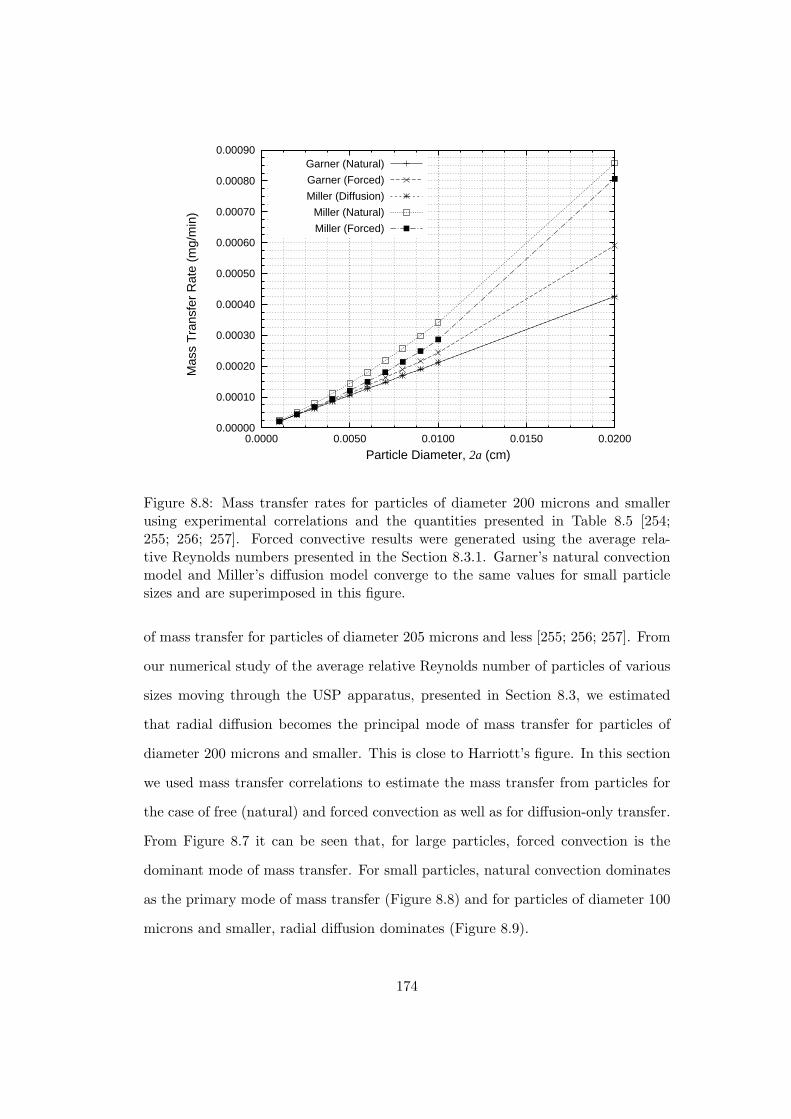
0.00000

0.00010

0.00020

0.00030

0.00040

0.00050

0.00060

0.00070

0.00080

0.00090

0.0000 0.0050 0.0100 0.0150 0.0200

Mas

s T

rans

fer

Rat

e (m

g/m

in)


Garner (Natural)

Garner (Forced)

Miller (Diffusion)

Miller (Natural)

Miller (Forced)

Figure 8.8: Mass transfer rates for particles of diameter 200 microns and smallerusing experimental correlations and the quantities presented in Table 8.5 [254;255; 256; 257]. Forced convective results were generated using the average rela-tive Reynolds numbers presented in the Section 8.3.1. Garner’s natural convectionmodel and Miller’s diffusion model converge to the same values for small particlesizes and are superimposed in this figure.

of mass transfer for particles of diameter 205 microns and less [255; 256; 257]. From

our numerical study of the average relative Reynolds number of particles of various

sizes moving through the USP apparatus, presented in Section 8.3, we estimated

that radial diffusion becomes the principal mode of mass transfer for particles of

diameter 200 microns and smaller. This is close to Harriott’s figure. In this section

we used mass transfer correlations to estimate the mass transfer from particles for

the case of free (natural) and forced convection as well as for diffusion-only transfer.

From Figure 8.7 it can be seen that, for large particles, forced convection is the

dominant mode of mass transfer. For small particles, natural convection dominates

as the primary mode of mass transfer (Figure 8.8) and for particles of diameter 100

microns and smaller, radial diffusion dominates (Figure 8.9).

174

0.00000

0.00010

0.00020

0.00030

0.00040

0.00050

0.00060

0.0000 0.0050 0.0100 0.0150 0.0200

Mas

s T

rans

fer

Rat

e (m

g/m

in)


Garner (Natural)

Garner (Forced)

Figure 8.9: Mass transfer rates for particles of diameter 200 microns and smallerusing only the experimental correlations of Garner [254] together with the quantitiespresented in Table 8.5. Forced convective results were generated using the averagerelative Reynolds numbers presented in the Section 8.3.1.

From Figure 8.8, we can see that there is no need to calculate the trajectory of

particles smaller than 100 microns through the USP apparatus as a radial diffusion

model [see e.g. 254; 257; 102] will be sufficiently accurate.

8.4 Errors and Additional Considerations

8.4.1 Calculation Stability

Results indicate that the relative Reynolds numbers for small particles are similar for

two-dimensional and three-dimensional flows. However, filling in the 3D data in this

region leads to the same recurring problem: the LPA/Euler and Verlet integration

schemes require ever smaller timesteps as the particle size decreases to maintain

stability. This means that for a given number of timesteps, the total simulation

time is reduced and the average Reynolds number is computed over smaller times.

175

It is useful to consider what causes this problem.

8.4.2 Effect of ts on Rep

It was observed that varying ∆t leads to different average relative Reynolds Num-

bers, Rep. This is sensible: as ts increases, Rep should converge on a fixed value.

It is also reasonable to think that this value will be different to Rep calculated over

shorter ts. This is because, for small simulated times, a particle will have moved

only a small distance through the velocity field and sudden changes in the velocity

field, i.e. high or low relative Reynolds Numbers, have a much larger effect on Rep

calculated over that period. For longer simulated times, Rep approaches a constant

as the simulated time increases.

8.4.3 Additional Assumptions and Shortcomings of the Models

8.4.4 Considering Many Particles

At present we have considered a single particle moving through simple velocity

fields. However, even with many drug particles moving in the USP apparatus,

the particles may be distributed sparsely enough to allow us still neglect particle-

particle interactions and particle-fluid effects. We do not have enough experimental

information yet to state this with confidence.

If this is not the case, i.e. particles are not distributed sparsely enough, then

there may be complicated interactions between the particles and the fluid and the

problems of particle motion and fluid motion may indeed be coupled. The problem

of calculating such fluid and particle motion within the USP apparatus is certainly

not a trivial one. This is further complicated by the fact that the particles dissolve

as they move through the fluid, meaning that a complete solution to the problem will

involve a multiphysics approach. A complete, detailed, solution that captures these

interactions is likely to require more sophisticated mathematical analysis, numerical

algorithms and computational implementations, e.g. parallel implementation. The

176

-0.06-0.04

-0.02 0

0.02 0.04

0.06-0.06

-0.04

-0.02

0

0.02

0.04

0.06

-0.06

-0.04

-0.02

0

0.02

0.04

0.06

0.08

Figure 8.10: When the timestep is too large, e.g. 1 second as shown here, the particlecovers almost half the width of the USP apparatus in one step. This quickly becomesunstable.

work set out here was to produce a useful model and a good foundation for future

development.

8.4.5 Analytical Limits

There is the possibility of running up against analytical limits. An analytical limit

in this context is understood to be the limit of a simulation’s ability to correctly

capture the physics of a process: when the simulation of a process begins to deviate

significantly from the actual process and the simulation is no longer valid. It is

certain that the simulations presented here, as with all simulations, do not capture all

177

the physics of the process we are investigating. This makes it all the more important

to have realistic expectations of the models’ capabilities and to understand their

limitations.


In summary, this chapter presented results from the last of the three studies de-

scribed in this thesis.

Calculations indicate that small particles move with the USP apparatus flow

and that, for particles with a diameter of approximately 0.01 cm (100 microns) and

smaller, radial diffusion is the dominant mode of mass transfer, i.e. forced convection

effects can be neglected for particles of diameter 100 microns and smaller. This result

is, it is believed, novel for the case of particle dissolution in the USP apparatus.

Importantly, this study contributes to the basis for arguing that simulation is useful

in the description of pharmaceutical processes.

8.5.1 Future Work

Proposed Complete Solution to the Problem of Drug Particle Dissolution

in the USP Type 2 Dissolution Apparatus

The aim of this work was to begin the development of a particle trajectory tracing

algorithm which can be used to predict the paths of and dissolution from tablet

fragments of various sizes moving in the USP Type 2 Dissolution Apparatus. In a

complete model, it is proposed that the initial drug particle size distribution could

be determined through the use of experimental data and a probabilistic model. The

particle motion and dissolution rate could be determined using classical particle

tracking techniques together with a simulated fluid velocity field. These components:

probabilistic model, particle tracking and a simulated velocity field, could together

form a complete model of drug fragmentation. Together with the work on the initial

178

dissolution rate, this could form part of a complete model of tablet dissolution.

Given a time-dependent distribution of particle sizes and a fluid velocity field, it

should be possible to estimate the overall dissolution rate of a tablet dissolving and

then fragmenting in a USP dissolution apparatus.

Outline of Probabilistic Component

A complete model of dissolution in a USP apparatus may require a probabilistic

component. As discussed previously, there is significant variability in the disso-

lution rates of tablets dissolving in this standard dissolution test apparatus. This

variability results from inherent factors in the operation of the dissolution apparatus

and in the tablet itself, i.e. tablets may or may not disintegrate into fragments and

those that do so will disintegrate at varying rates. The idea is that the probabilistic

component, which may use an Inverse Monte Carlo technique in a Bayesian frame-

work, adjusts the model at each time-step using a probable distribution of fragment

sizes informed by and validated against concentration measurements and other data

from experiment. This is based on previous work, e.g. [112; 113]. After each run,

the distribution of particle sizes is corrected using an Inverse MC method.

A Possible Inverse Monte-Carlo Method

If a key result, e.g. the mass transfer rate, from the model is M(x) and the true,

measured, value from the physical system is denoted MTrue, then the error Esys

between the simulated and actual systems will be M −MTrue = Esys. If a set of n

values for M is obtained for n different x values, the Euclidean distance between

the simulated and true values can be calculated for each instance. Instances with

small distances are most likely. This information can be used to determine which

possible combinations of system parameters are most useful and this, in turn, can

be used to set these parameters so that further predictions can be made for a new

set of initial conditions.

179

Chapter 9

Summary, Future Work and

Conclusions

9.1 Summary

9.1.1 Study 1

The first study developed the understanding of quasi-steady drug dissolution from

the surface of a multi-layered tablet in the USP apparatus. A Crank-Nicolson finite-

difference approximation to the drug mass transfer rate from dissolving cylindrical

tablets, consisting of alternating layers of drug and inert material, was presented and

results were compared with recent solutions to the same problem and with previous

experimental results produced using the USP apparatus. It was shown that (i) the

theoretical estimates differ by up to 10%, a result of different implementations of a

derivative surface boundary condition, (ii) the new finite-difference model is more

physically realistic but that the recent analytical solution of Crane et al is shown to

be usefully accurate. In addition, it was established that the assumption of a steady,

axial mainstream flow is likely to be the primary reason for the error between the

experimental and theoretical results.

180

9.1.2 Study 2

The second study investigated the flow around the top of a cylinder using a com-

mercial fluid dynamics code. A specific application to a complementary problem

in wind energy was considered. In addition to other sources of error, accelerated

airflow, or speed-up, around the top of cylindrical meteorological (met) towers can

cause incorrect wind-speed measurements. A particular configuration was consid-

ered where the anemometer was located only two tower diameters above a met

tower. Using a standard computational fluid dynamics package, the maximum error

for this configuration was found to be 2% of the wind-speed. It was concluded that

top-mounted anemometers should be located at the windward side of a meteorolog-

ical tower, where a particular wind direction prevails, and at least five diameters

above the top. This will reduce speed-up to less that 1%. The IEA recommenda-

tion is for a minimum separation of about 6 tower diameters [203]. In line with the

IEA’s recommendation that the anemometer installation should be ‘clean’ [203], it

is recommended that towers should be made from a corrosion resistant material and

maintained and cleaned regularly to minimise flow disturbance.

9.1.3 Study 3

The third part of this work considered one possible end state for a dissolving tablet:

fragmentation into small particles with dissolution continuing from the disintegrated

solid masses. A framework for calculating the motion of and dissolution from a drug

particle moving through the USP apparatus was outlined, beginning with a review

of the classical work of Taylor and Glauert, who considered the motion of raindrops

in airflows. Calculations indicate that small particles move with the USP apparatus

flow and that, for particles of diameter of approximately 0.01 cm (100 microns) and

smaller, radial diffusion is the dominant mode of mass transfer, i.e. forced convection

effects can be neglected for particles of diameter 100 microns and smaller.

181

9.2 Future Work

The potential areas of research arising from this thesis are many. Specific and

general suggestions include:

9.2.1 Specific Research Questions

Arising from Study 1

Future developments of this work must incorporate boundary-layer theory close to

the surface using a more realistic free-stream velocity field, ideally calculated con-

currently using a computational fluid dynamics code. Further research may also

include: (i) exploring the limits of validity for the Pohlhausen solution, to further

clarify the reasons for its deviation from the CN solution and to formally demon-

strate that its convergence as the number of layers becomes very large can be written

in a closed form; (ii) formulating other applications for the extended Pohlhausen so-

lution. This may have some utility when considering matrix tablets, i.e. a large

number of layers may approximate matrix tablet behaviour. Other applications

might include microelectrode analysis; (iii) the CN finite-difference method can be

extended in many ways including the already mentioned consideration of more re-

alistic flows from a coupled CFD code. There are many outstanding investigations

around the CN scheme, including, e.g. detailed investigations of its validity and

incorporation of more efficient mesh distributions.


Future work arising from the second study may include, in the area of wind energy,

several essential refinements of the work presented; these include extending the

analysis for different tower and anemometer configurations and for different tower

types, e.g. considering the error in wind-speed measurements from anemometers

mounted close to the side of a meteorological tower. Another useful study will be to

182

use more sophisticated turbulence models and to carry out a more complete study

of the effect of turbulence on the wind-speed close to the tower. The use of similar

techniques to examine the mass transfer from a cylindrical tablet in cross-flow may

also be a useful avenue of research.


Many research directions arise from the particle tracking work. These include (i)

developing a more sophisticated CGNS based code (ii) investigating OpenFOAM

as a platform for conducting this work, (iii) using more sophisticated algorithms

which incorporate particle-particle interactions and so forth in particle tracking,

(iv) considering a parallel version of the code and (v) integrating this work with a

probabilistic framework.

9.3 Conclusions

The three main studies, (1) quasi-steady drug dissolution from a multi-layered tablet

in the USP apparatus, (2) flow distortion about a cylinder and (3), the mass transfer

from small particles moving in the USP apparatus, each form a part of a future

complete framework for simulating drug dissolution in the USP apparatus. These

investigations were consistent with our aim of building on earlier understanding of

drug dissolution in the USP apparatus and to demonstrate the thesis that simulation

has the potential to be of significant use for pharmaceutics.

183

Bibliography

[1] F. Norton, The art of writing scientific reports, TM 7, NACA (1921).

[2] A. Roland, Model Research, NASA, Scientific and Technical Information

Branch, Washington, D.C., 1985, Ch. Volume 2, Appendix F, Research Au-

thorization 201.

URL http://history.nasa.gov/SP-4103/contents.htm

[3] R. Langer, Drug delivery and targeting, Nature (392) (1998) 5 – 10, (Supp).

[4] IBM Business Consulting Services, Pharma 2010: The threshold of innovation,

Executive brief, IBM Institute for Business Value (2004).

[5] H. A. Mucke, A new paradigm for clinical development: The clinical trial in

2015, Advances in Life Sciences Reports 58, Cambridge Healthtech Advisors

(CHA) (2005).

[6] D. E. Leahy, Drug discovery information integration: virtual humans for phar-

macokinetics, Biosilico 2 (2) (2004) 78–84.

[7] M. Aulton, Pharmaceutics, the Science of Dosage Form Design, 2nd Edition,

Churchill-Livingstone, Edinburgh etc., 2002.

[8] V. Pillay, R. Fassihi, Unconventional dissolution methodologies, J. Pharm.

Sci. 88 (9) (2000) 843 – 851.

184

[9] T. Mirza, Y. Joshi, Q. Liu, R. Vivilecchia, Evaluation of Dissolution Hydrody-

namics in the USP, Peaktm and Flat-Bottom Vessels Using Different Solubility

Drugs, Tech. rep., Diss. Tech., Article 2 (Feb 2005).

[10] United States Pharmacopeial Convention, USP-NF 24, 19th Edition,

Rockville, MD, 2000, Ch. Dissolution <711>, p. 1941.

[11] W. Higuchi, N. Mir, S. Desai, Dissolution rates of polyphase mixtures, J.

Pharm. Sci. 54 (1965) 1405 – 1410.

[12] A.-M. Healy, O. Corrigan, The influence of excipient particle size, solubility

and acid strength on the dissolution of an acidic drug from two-component

compacts, Int. J. Pharm. 143 (1996) 211–221.

[13] Z. Ramtoola, O. Corrigan, Dissolution characteristics of benzoic acid and sali-

cylic acid mixtures in reactive Media, Drug Dev. Ind. Pharm. 13 (1987) 1703–

1720.

[14] A.-M. Healy, O. Corrigan, Predicting the dissolution rate of ibuprofen-acidic

excipient compressed mixtures in reactive media, Int. J. Pharm. 84 (2) (1992)

167–173.

[15] S. A. Qureshi, J. Shabnam, Cause of high variability in drug dissolution testing

and its impact on setting tolerances, Eur. J. Pharm. Sci. 12 (3) (2001) 271 –

276.

[16] J. Kukura, J. Baxter, F. Muzzio, Shear distribution and variability in the USP

Apparatus 2 under turbulent conditions, Int. J. Pharm. 279 (1-2) (2004) 9 –

17.

[17] M. Crane, N. J. Hurley, L. Crane, A.-M. Healy, O. I. Corrigan, K. M. Gal-

lagher, L. G. McCarthy, Simulation of the USP drug delivery problem us-

185

ing CFD: Experimental, numerical and mathematical aspects, Simul. Model.

Pract. Th. 12 (2) (2004) 147–158.

[18] J. Baxter, J. Kukura, F. Muzzio, Hydrodynamics-induced variability in the

USP apparatus II dissolution test, Int. J. Pharm. 292 (1-2) (2005) 17–28.

[19] D. D’Arcy, O. Corrigan, A. Healy, Hydrodynamic simulation (computational

fluid dynamics) of asymmetrically positioned tablets in the paddle dissolution

apparatus: impact on dissolution rate and variability, J. Pharm. Pharmacol.

57 (10) (2005) 1243 – 1250(8).

[20] PSUDO, Final report, Tech. rep., Parallel Simulation of Drug release code

(PSUDO) Project (2000).

URL http://icetact.tchpc.tcd.ie/icetact/examples/PSUDOfinal.

html

[21] M. Crane, L. Crane, A.-M. Healy, O. Corrigan, K. Gallagher, L. McCarthy,

A Pohlhausen Solution for the Mass Flux From a Multi-layered Compact in

the USP Drug Dissolution Apparatus, Simul. Model. Pract. Th. 12 (6) (2004)

397–411.

[22] G. Taylor, Notes on possible equipment and technique for experiments on icing

on aircraft, ARC R & M 2024.

[23] M. Glauert, A Method of Constructing the Paths of Raindrops of Different

Diameters moving in the neighbourhood of (1) a Circular Cylinder, (2) an

Airfoil, placed in a Uniform Stream of Air ; and a Determination of the Rate

of Deposit of Drops on the Surface and the Percentage of Drops Caught, ARC

R & M 2025.

[24] Int. J. Pharm., Journal Information, Product Description [Online], Int. J.

Pharm.[Viewed 15 March 2006].

URL www.elsevier.com/locate/ijpharm/

186

[25] R. Borchardt, A. Repta, V. Stella, Directed Drug Delivery: A Multidisci-

plinary Problem, Humana Press, Clifton, NJ, USA, 1985, Ch. 1.

[26] J. R. Robinson, Pharmaceutics and the evolving technology of drug delivery -

a perspective, in: R. T. Borchardt, A. J. Repta, V. J. Stella (Eds.), Directed

Drug Delivery, a Multidisciplinary Problem, Humana Press, New Jersey, 1984.

[27] J. Drews, Drug discovery: A historical perspective, Science 287 (2000) 1960–

1964.

[28] R. Langer, Where a pill won’t reach, Sci. Am. 288 (4) (2003) 32 – 39.

[29] R. Langer, Langer discusses drug delivery advances at AMA briefing, MIT

News Office [Accessed March 15 2006].

URL http://web.mit.edu/newsoffice/2004/langer.html

[30] V. J. Stella, My mentors, J. Pharm. Sci. 90 (2001) 969–978.

[31] R. L. Juliano, Drug Delivery Systems - Characteristics and Biomedical Appli-

cations, Oxford University Press, New York, Oxford, 1980, Ch. 1.

[32] R. Langer, Polymer-controlled drug delivery systems, Accounts Chem. Res.

26 (1993) 537–542.

[33] S. Abdul, S. Poddar, A flexible technology for modified release of drugs: multi

layered tablets, J. Control. Release 97 (3) (2004) 393–405.

[34] GlaxoSmithKline, Our history (Webpage), [Online, accessed 13th February

2006] (2006).

URL http://www.gsk.com/about/history.htm

[35] R. Blythe, Sympathometic preparation, United States Patent and Trademark

Office, Patent 2,738,303 (March 13, 1956).

187

[36] M. Gohel, M. Panchal, Quantitative expression of deviation from zero-order

drug release, Pharmaceutical Technology 25 (9) (2001) 62–74.

[37] J. Siepmann, A. Gopferich, Mathematical modeling of bioerodible, polymeric

drug delivery systems, Adv. Drug Deliver. Rev. 48 (2-3) (2001) 229–247.

[38] A. Streubel, J. Siepmann, N. A. Peppas, R. Bodmeier, Bimodal drug release

achieved with multi-layer matrix tablets: transport mechanisms and device

design, J. Control. Release 69 (3) (2000) 455–468.

[39] U. Conte, L. Maggi, P. Colombo, A. La Manna, Multi-layered hydrophilic ma-

trices as constant release devices (Geomatrixtm systems), J. Control. Release

26 (1) (1993) 39–47.

[40] Y. Qiu, N. Chidambaram, K. Flood, Design and evaluation of layered diffu-

sional matrices for zero-order sustained release, J. Control. Release 51 (2-3)

(1998) 123–130.

[41] U. Conte, L. Maggi, Modulation of the dissolution profiles from Geomatrix

multi-layer matrix tablets containing drugs of different solubility, Biomaterials

17 (1996) 889–896.

[42] SkyePharma, Geomatrix, [Online], [10 November 2006] (2006).

URL http://www.skyepharma.com/oral.html

[43] S. A. Qureshi, I. J. McGilveray, Typical variability in drug dissolution testing:

study with USP and FDA calibrator tablets and a marketed drug (gliben-

clamide) product, Eur. J. Pharm. Sci. 7 (1999) 249 – 258.

[44] L. McCarthy, G. Bradley, J. Sexton, O. Corrigan, A. Healy, Computational

fluid dynamics modeling of the paddle dissolution apparatus: Agitation rate,

mixing patterns, and fluid velocities, AAPS PharmSciTech 5 (2).

188

[45] Y. Wu, O. Kildsig, E. Ghaly, Effect of hydrodynamic environment on tablets

dissolution rate, Pharm. Dev. Technol. 9 (1) (2004) 25 – 37.

[46] Tufts Center for the Study of Drug Development, Tufts center for the study

of drug development pegs cost of a new prescription medicine at $802 million,

Press Release.

URL http://csdd.tufts.edu/NewsEvents/RecentNews.asp?newsid=6

[47] M. Dickson, J. Gagnon, Key factors in the rising cost of new drug discovery

and development, Nat. Rev. Drug Discov. 3 (2004) 417 – 429.

[48] J. DiMasi, R. Hansen, H. Grabowski, The price of innovation: new estimates

of drug development costs, J. Health Econ. 22 (2) (2003) 151–185.

[49] R. G. Frank, New estimates of drug development costs, J. Health Econ. 22

(2003) 325–330.

[50] R. Mullin, Drug development costs about $1.7 billion, Chemical & Engineering

News 81 (50) (2003) 8.

URL http://pubs.acs.org/cen/topstory/8150/8150notw5.html

[51] J. DiMasi, Risks in new drug development: Approval success rates for inves-

tigational drugs, Clin. Pharmacol. Ther. 69 (5) (2001) 297–307.

[52] G. M. Grass, P. J. Sinko, Physiologically-based pharmacokinetic simulation

modelling, Adv. Drug Deliver. Rev. 54 (2) (2002) 433–451.

[53] PhRMA, What goes into the cost of prescription drugs?, Report, The Phar-

maceutical Research and Manufacturers of America (PhRMA) (June 2005).

URL http://www.phrma.org/files/Cost_of_Perscription_Drugs.pdf

[54] C. George, J. M. Pearson, Riding the pharma roller coaster, The McKinsey

Quarterly (4).

189

[55] Food and Drug Administration, Drug Approval Application Process, Website,

U.S. Department of Health and Human Services (2006).

URL http://www.fda.gov/cder/regulatory/applications/

[56] M. Pandey, Investment decisions in pharmaceutical R&D projects, Drug Dis-

cov. Today 8 (21) (2003) 968–971.

[57] European Medicines Agency (EMEA), Questions and answers on recommen-

dation for refusal of marketing application for Atryn, Press Release, document

reference: EMEA/62022/2006 (February 2006).

[58] M. Peplow, Drug from GM animal gets thumbs down, Nature [Online].

URL doi:10.1038/news060220-17

[59] K. Honey, The comeback kid: TYSABRI now FDA approved for Crohn dis-

ease, J. Clin. Invest. 118 (3) (2008) 825–826.

URL http://dx.doi.org/10.1172/JCI35179

[60] Food and Drug Administration, Natalizumab (marketed as Tysabri) informa-

tion (2005) 825–826.

URL http://www.fda.gov/cder/drug/infopage/natalizumab/default.

htm

[61] W. Russell, R. Burch, The Principles of Humane Experimental Technique,

Methuen & Co, London, 1959.

[62] S. Laville, One year on from schoolboy’s fightback, animal rights activists are

forced to rethink tactics, The Guardian (2007) February 26.

URL http://www.guardian.co.uk/animalrights/story/0,,2021453,00.

html

[63] F. P. Gruber, T. Hartung, Alternatives to Animal Experimentation in Basic

Research, ALTEX Archive Sup. 1 (1) (2004) .

190

[64] V. Robinson, Finding alternatives: an overview of the 3Rs and the use of

animals in research, School Science Review 87 (2005) 319.

[65] European Union, Seventh Framework Programme for Research.

URL http://cordis.europa.eu/fp7/home_en.html

[66] D. R. Chapman, H. Mark, M. W. Pirtle, Computers vs. wind tunnels for

aerodynamic flow simulations, Astronaut. Aeronaut. 13 (1975) 22–35.

[67] E. A. Muenger, Searching the Horizon, A History of Ames Research Center

1940-1976, Scientific and Technical Information Branch, NASA, Washington,

D.C., 1985.

URL http://history.nasa.gov/SP-4304/sp4304.htm

[68] T. C. Bickel, H. Morgan, C. Peterson, Applications of computational me-

chanics at Sandia National Laboratories, in: Computational fluid and solid

mechanics, 2005, Proceedings of the Third M.I.T. Conference on Computa-

tional Fluid and Solid Mechanics, held in Cambridge, Massachusetts, USA,

June 14 - 17, 2005.

[69] A. Jameson, The Role of CFD in Preliminary Aerospace Design, in: 4th

ASME-JSME Joint Fluids Engineering Conference, Honolulu, Hawaii, 2003.

[70] C. A. Fletcher, Computational Techniques for Fluid Dynamics 1: Fundamen-

tal and General Techniques, 2nd Edition, Springer-Verlag, Berlin, 1991, 6th

Printing, 2005.

[71] IBM Business Consulting Services, Pharma 2005: Silicon rally, the race to

e-R&D, Report, IBM Global Services, Originally published in 1999 by Price-

waterhouseCoopers (PwC) (2002).

[72] B. Ataie-Ashtiani, S. Hosseini, The completed human genome: implications

for chemical biology, Curr. Opin. Chem. Biol. 7 (4) (2003) 511–515.

191

[73] C. A. Hunt, S. Guzy, D. L. Weiner, A forecasting approach to accelerate drug

development, Stat. Med. 17 (15-16) (1998) 1725–1740.

[74] S.-S. Feng, S. Chien, Chemotherapeutic engineering: Application and further

development of chemical engineering principles for chemotherapy of cancer

and other diseases, Chem. Eng. Sci. 58 (2003) 4087–4114.

[75] Entelos, Inc., Entelos Announces U.S. Patent for the Development and Use of

Virtual Patients, Press Release.

URL http://www.entelos.com/news/pressArchive/press72.html

[76] T. S. Paterson, A. L. Bangs, Method and apparatus for conducting linked

simulation operations utilizing a computer-based system model, United States

Patent and Trademark Office, Patent 6,983,237 (US2006031059) (February 9,

2006).

[77] D. Teather, Virtual patient firm opts for Aim, The Guardian (2006) March

7.

URL http://business.guardian.co.uk/story/0,,1725167,00.html

[78] J. Russell, Optimizing Optimata, Bio-IT World (November 15, 2005).

URL http://www.bio-itworld.com/issues/2005/nov/

russell-transcript/

[79] K. Skomorovski, H. Harpak, A. Ianovski, M. Vardi, T. P. Visser, S. C. Hartong,

H. H. van Vliet, G. Wagemaker, Z. Agur, New TPO treatment schedules

of increased safety and efficacy: pre-clinical validation of a thrombopoiesis

simulation model, Brit. J. Haematol. 123 (4).

[80] P. Wellstead, Schrodinger’s legacy: Systems and life, An E.T.S. Walton

Lecture given as part of the W.R. Hamilton Bi-Centenary Lecture Series,

The Royal Irish Academy (April 2005).

192

URL http://www.hamilton.ie/systemsbiology/files/2005/

schroedinger.pdf

[81] G. S. Mack, Can complexity be commercialized?, Nat. Biotechnol. 22 (2004)

1223–1229.

[82] W. Russell, R. Burch, The Principles of Humane Experimental Technique,

2nd Edition, Universities Federation for Animal Welfare, Hertfordshire, 1992.

URL http://altweb.jhsph.edu/publications/humane_exp/het-toc.htm

[83] NC3Rs, The 3Rs, [Online], [April 18th 2006] (2006).

URL http://www.nc3rs.org.uk/

[84] The Human Genome Program, Genome Programs of the U.S. Department of

Energy Office of Science, Website, U.S. Department of Energy Office of Science

(2006).

URL http://www.doegenomes.org/

[85] E. Crampin, M. Halstead, P. Hunter, P. Nielsen, N. Noble, D amd Smith,

M. Tawhai, Computational physiology and the physiome project, Exp. Phys-

iol. 89 (1) (2004) 1 – 26.

[86] G. L.-T. Chiu, M. Gupta, A. K. Royyuru, Blue Gene, Preface, IBM J. Res.

Dev. 49 (2/3).

URL doi:10.1147/rd.492.0191

[87] A. Noyes, W. Whitney, The Rate of Solution of Solid Substances in their own

Solutions, J. Am. Chem. Soc. 19 (1897) 930–934.

[88] J. Wang, D. R. Flanagan, General Solution for Diffusion-Controlled Dissolu-

tion of Spherical Particles. 1. Theory, J. Pharm. Sci. 88 (7) (1999) 731–738.

[89] L. Prandtl, Motion of fluids with very little viscosity, TM 452, NACA (1928).

193

[90] W. Nernst, Theorie der Reaktionsgeschwindigkeit in Heterogenen Systemen,

Z. Physik. Chem. 47 (1904) 52–55.

[91] E. Brunner, Reaktionsgeschwindigkeit in Heterogenen Systemen, Z. Physik.

Chem. 47 (1904) 56–102.

[92] C. V. King, Reaction rates at solid–liquid interfaces, J. Am. Chem. Soc. 57

(1935) 828–831.

[93] L. Prandtl, Uber Flussigkeitsbewegung bei sehr kleiner Reibung, Verh. III.

Intern. Math. Kongr., Heidelberg, 1904 (1905) 484–491.

[94] J. Crank, Mathematics of Diffusion, 2nd Edition, Oxford University Press,

Oxford, 1975.

[95] C. C. Sun, Quantifying errors in tableting data analysis using the Ryshkewitch

equation due to inaccurate true density, J. Pharm. Sci. 94 (2005) 2061–2068.

[96] S. W. Yu, L. J. van Vliet, H. W. Frijlink, K. van der Voort Maarschalk, The

determination of relative path length as a measure for tortuosity in compacts

using image analysis, Eur. J. Pharm. Sci. 28 (5) (2006) 433–440.

[97] P. J. O’Dowd, O. I. Corrigan, Dissolution kinetics of three component non-

disintegrating compacts: theophylline, benzoic acid and salicylamide, Int. J.

Pharm. 176 (2) (1999) 231–240.

[98] B. Killen, O. Corrigan, Factors influencing drug release from stearic acid based

compacts, Int. J. Pharm. 228 (1-2) (2001) 189–98.

[99] E. Kenny, A moving boundary finite element solution of a pharmaceutical drug

delivery problem, Msc. thesis, Trinity College, University of Dublin (1994).

[100] Hitachi Europe, European Esprit grant awarded to Hitachi Dublin Laboratory

& Trinity College Dublin, Press Release (August 1998).

URL http://www.hitachi.com/New/cnews/E/1998/980820B.html

194

[101] C. Vuik, C. Cuvelier, Numerical solution of an etching problem, J. Comput.

Phys. 59 (1985) 247–263.

[102] F. P. Incropera, D. P. DeWitt, Fundamentals of Heat and Mass Transfer, Fifth

Edition, John Wiley & Sons, New York, 2002.

[103] P. Scott, Geometric irregularities common to the dissolution vessel, Diss. Tech.

12 (1) (2005) 18–21.

[104] A.-M. Healy, L. McCarthy, K. Gallagher, O. Corrigan, Sensitivity of dissolu-

tion rate to location in the paddle dissolution apparatus, J. Pharm. Pharmacol.

54 (3) (2002) 441–444.

[105] L. McCarthy, C. Kosiol, A.-M. Healy, G. Bradley, J. Sexton, O. Corrigan,

Simulating the Hydrodynamic Conditions in the United States Pharmacopeia

Paddle Dissolution Apparatus, AAPS PharmSciTech 4 (2).

[106] Fluent Inc., FLUENT User’s Guide, Lebanon, NH, USA (2003).

[107] A. Leveque, Les lois de la transmission de chaleur par convection, Ann. des

Mines Memoires, Tome XIII (13) (1928) 201 – 239.

[108] J. Kestin, L. Persen, The transfer of heat across a turbulent boundary layer

at very high Prandtl numbers, Int. J. Heat Mass Tran. 5 (1962) 355–371.

[109] R. Seban, R. Bond, Skin friction and heat transfer characteristics of a laminar

boundary layer on a cylinder in axial flow, J. Aeronaut. Sci. 18 (1951) 671–675.

[110] L. Verlet, Computer “Experiments” on Classical Fluids. I. Thermodynamical

Properties of Lennard-Jones Molecules, Phys. Rev. 159 (1) (1967) 98.

[111] A. Tarantola, Inverse Problem Theory and Methods for Model Parameter

Estimation, Society for Industrial and Applied Mathematics, Philadelphia,

PA, USA, 2004.

195

[112] A. Barat, H. J. Ruskin, M. Crane, Probabilistic models for drug dissolution.

Part 1. Review of Monte Carlo and stochastic cellular automata approaches,

Simul. Model. Pract. Th. 14 (2006) 843–856.

[113] A. Barat, H. J. Ruskin, M. Crane, Probabilistic methods for drug dissolution.

Part 2. Modelling a soluble binary drug delivery system dissolving in vitro,

Simul. Model. Pract. Th. 14 (2006) 857–873.

[114] F. White, Viscous Fluid Flow, 2nd Edition, McGraw-Hill, New York, 1991.

[115] H. Schuh, A new method for calculating laminar heat transfer on cylinders of

arbitrary cross-section and on bodies of revolution at constant and variable

wall temperature, TN 33, KTH Aero (1954).

[116] H. Schuh, On asymptotic solutions for the heat transfer at varying wall tem-

peratures in a laminar boundary layer with Hartree’s velocity profiles, J. Aero.

Sci. 20(2) (1953) 146–147.

[117] H. Schlichting, Boundary-Layer Theory, 7th Edition, McGraw-Hill, New York,

1979.

[118] H. Martin, The Generalized Leveque Equation And Its Practical Use For The

Prediction Of Heat And Mass Transfer Rates From Pressure Drop, Chem.

Eng. Sci. 57 (16) (2002) 3217–3223.

[119] S.-C. Chang, J. Jin, Computation of special functions, 2nd Edition, Wiley-

Interscience, New York, 1996.

[120] M. Dehghan, Weighted finite difference techniques for the one-dimensional

advection-diffusion equation, Appl. Math. Comput. 147 (2004) 307 – 319.

[121] J. Alden, Computational electrochemistry, Ph.D. thesis, Oxford University

(1998).

URL http://physchem.ox.ac.uk/~rgc/john/Thesis/

196

[122] M. Dehghan, Numerical solution of the three-dimensional advection-diffusion

equation, Appl. Math. Comput. 150 (2004) 5 – 19.

[123] M. Dehghan, Numerical schemes for one-dimensional parabolic equations with

nonstandard initial condition, Appl. Math. Comput. 147 (2004) 321–331.

[124] B. Laval, B. R. Hodges, J. Imberger, Numerical Diffusion in Stratified Lake

Models, Proc. 5th Intl. Symposium on Stratified Flows, Vancouver July 7-11,

2000.

[125] B. Ataie-Ashtiani, D. Lockington, R. Volker, Truncation errors in finite differ-

ence models for solute transport equation with first-order reaction, J. Contam.

Hydrol. 35 (1999) 409–428.

[126] J. Liu, E. S. Oran, C. R. Kaplan, Numerical diffusion in the FCT algorithm,

revisited, J. Comp. Phys. 208 (2005) 416434.

[127] R. F. Warming, B. J. Hyett, The modified equation approach to the stability

and accuracy analysis of finite-difference methods, J. Comput. Phys. 14 (2)

(1974) 159–179.

[128] J. Alden, J. Booth, R. G. Compton, R. A. Dryfe, G. H. Sanders, Diffusional

mass transport to microband electrodes of practical geometries: A simulation

study using the strongly implicit procedure, J. Electroanal. Chem. 389 (1-2)

(1995) 45–54.

[129] M. Dehghan, Quasi-implicit and two-level explicit finite-difference procedures

for solving the one-dimensional advection equation, Appl. Math. Comput. 167

(2005) 46–67.

[130] V. Vemuri, W. J. Karplus, Digital Computer Treatment of Partial Differential

Equations, Prentice-Hall, New Jersey, 1981.

197

[131] L. Chung-Yau, Applied Numerical Methods for Partial Differential Equations,

Prentice Hall [Simon and Schuster (Asia) Pte Ltd.], Singapore, 1994.

[132] M. Thompson, O. V. Klymenko, R. G. Compton, Modelling homogeneous

kinetics in the double channel electrode, J. Electroanal. Chem. 576 (2) (2005)

333 – 338.

[133] C. J. Freitas, Editorial policy statement on the control of numerical accuracy,

ASME J. Fluids Eng. 115 (1993) 339–340.

URL http://journaltool.asme.org/Templates/JFENumAccuracy.pdf

[134] D. Britz, Investigation into the relative merits of some n-point current approx-

imations in digital simulation, Anal. Chim. Acta 193 (1987) 277–285.

[135] D. E. Knuth, Big omicron and big omega and big theta, SIGACT News 8 (2)

(1976) 18–24.

[136] D. Gavaghan, How accurate is your two-dimensional numerical simulation?

Part 1. an introduction, J. Electroanal. Chem. 420(1-2) (1997) 147–158.

[137] L. Ehrlich, A numerical method of solving a heat flow problem with moving

boundary, J. ACM 5 (1958) 161–176.

[138] L. Thomas, Elliptic problems in linear difference equations over a network,

Watson Sci. Comput. Lab. Report, Columbia University (1949).

[139] G. Bruce, D. Peaceman, Rachford, H. H. Jr., Rice, J.D., Calculations of

unsteady-state gas flow through porous media, Petroleum Transactions, AIME

198 (1953) 79–92.

[140] W. J. Minkowycz, G. E. Schneider, R. H. Pletcher, E. M. Sparrow, Handbook

of Numerical Heat Transfer, John Wiley & Sons, Inc., New York etc., 1988.

[141] A. C. Fisher, R. G. Compton, Chronoamperometry at Channel Electrodes: A

General Computational Approach, J. Phys. Chem. 95 (19) (1991) 7538–7542.

198

[142] C. J. Freitas, The issue of numerical uncertainty, App. Math. Model. 26 (2002)

237–248.

[143] J. Zhu, H. Guowei, Error estimation and uncertainty propagation in compu-

tational fluid mechanics, ICASE Interim Report 41, NASA (2002).

[144] I. Celik, Procedure for estimation and reporting of discretization error in CFD

applications, in: C. Freitas (Ed.), Editorial Policy Statement on the Control

of Numerical Accuracy, J. Fluids Eng., 2005.

URL http://journaltool.asme.org/Templates/JFENumAccuracy.pdf

[145] W. L. Oberkampf, Discussion: ‘Comprehensive Approach to Verification and

Validation of CFD Simulations - Part 1: Methodology and Procedures’ (Stern,

F., Wilson, R. V., Coleman, H. W., and Paterson, E. G., 2001, ASME J. Fluids

Eng., 123, pp. 793802), ASME J. Fluid Eng. 124(3) (2002) 809–810.

[146] F. Stern, H. W. Coleman, E. G. Paterson, Comprehensive Approach to Veri-

fication and Validation of CFD Simulations - Part 1: Methodology and Pro-

cedures, J. Fluid. Eng. - T. ASME 123(4) (2000) 793–802.

[147] American Institute of Aeronautics and Astronautics, Recommended Practice

for The CFD General Notation System - Standard Interface Data Structures

(AIAA R-101-2002), AIAA Standards Series (2002).

[148] B. H. Thacker, ASME standards committee on verification and validation in

computational solid mechanics, Report, The American Society of Mechanical

Engineers (ASME) Council on Codes and Standards (Sep 2001).

[149] I. Celik, Numerical uncertainty in fluid flow calculations: Needs for future

research, J. Fluid Eng. 115 (1993) 194 – 195.

[150] L. F. Richardson, The Approximate Arithmetical Solution by Finite Differ-

ences of Physical Problems Involving Differential Equations, with an Applica-

199

tion to the Stresses in a Masonry Dam, Philos. T. R. Soc. A 210 (1911) 307 –

357.

[151] L. F. Richardson, J. A. Gaunt, The Deferred Approach to the Limit. Part

I. Single Lattice. Part II. Interpenetrating Lattices, Philos. T. R. Soc. A 226

(1927) 299 – 361.

[152] I. Celik, J. Li, G. Hu, C. Shaffer, Limitations of Richardson Extrapolation and

Some Possible Remedies, J. Fluids Eng. 127(4) (2005) 795–805.

[153] W. L. Oberkampf, T. G. Trucano, Verification and validation in computational

fluid dynamics, Prog. Aerosp. Sci. 38 (2002) 209 – 272.

[154] W. L. Oberkampf, T. G. Trucano, C. Hirsch, Verification, validation, and

predictive capability in computational engineering and physics, SAND

REPORT SAND2003-3769, Sandia (2003).

URL http://www.prod.sandia.gov/cgi-bin/techlib/access-control.

pl/2002/023769.pdf

[155] D. Britz, Brute force digital simulation, J. Electroanal. Chem. 406 (1-2) (1996)

15–21.

[156] D. Britz, Stability of the backward differentiation formula (firm) applied to

electrochemical digital simulation, Comput. Chem. 21 (2) (1997) 97–108.

[157] D. Britz, O. Østerby, J. Strutwolf, Damping of Crank-Nicolson error oscilla-

tions, Comp. Bio. Chem. 27 (3) (2003) 253–263.

[158] J. A. Cooper, R. G. Compton, Channel electrodes - a review, Electronanal.

10 (3) (1998) 141 – 155.

[159] R. Ferrigno, P. F. Brevet, H. H. Girault, Finite element simulation of the

chronoamperometric response of recessed and protruding microdisc electrodes,

Electrochim. Acta 42 (12) (1997) 1895–1903.

200

[160] W. Zhang, H. Stone, J. Sherwood, Mass transfer at a microelectrode in channel

flow, J. Phys. Chem. 100 (1996) 9462–9464.

[161] N. P. Stevens, A. C. Fisher, Finite Element Simulations in Electrochemistry.

2. Hydrodynamic Voltammetry, J. Phys. Chem. B 101 (1997) 8259–8263.

[162] N. V. Rees, R. A. W. Dryfe, J. A. Cooper, B. A. Coles, R. G. Compton, S. G.

Davies, T. D. McCarthy, Voltammetry under High Mass Transport Condi-

tions. A High Speed Channel Electrode for the Study of Ultrafast Kinetics, J.

Phys. Chem. 99 (18) (1995) 7096–7101.

[163] P. Laasonen, Uber eine Methode zur Losung der Warmeleitungs-gleichung,

Acta Math-Djursholm 81 (1949) 309–317.

[164] R. G. Compton, B. A. Coles, A. C. Fisher, Chronoamperometry at Channel

Electrodes: Theory of Double-Electrodes, J. Phys. Chem. 98 (9) (1994) 2441–

2445.

[165] R. G. Compton, R. A. Dryfe, R. G. Wellington, J. Hirst, Modelling electrode

reactions using the strongly implicit procedure, J. Electroanal. Chem. 383 (1-

2) (1995) 13–19.

[166] J. Galceran, D. J. Gavaghan, J. S. Rollett, Two-dimensional implementation

of the finite element method with singularity correction for diffusion limited

current at an unshielded disc electrode, J. Electroanal. Chem. 394 (1-2) (1995)

17–28.

[167] C. Amatore, I. Svir, A new and powerful approach for simulation of diffusion at

microelectrodes based on overlapping sub-domains: application to chronoam-

perometry at the microdisk, J. Electroanal. Chem. 557 (2003) 75–90.

[168] D. Gavaghan, J. Rollett, Correction of boundary singularities in numerical

201

simulation of time-dependent diffusion processes at unshielded disc electrodes,

J. Electroanal. Chem. 295 (1990) 1–14.

[169] H. Motz, The Treatment of Singularities of Partial Differential Equations by

Relaxation Methods, Quart. Appl. Maths IV (4) (1946) 371–377.

[170] L. Woods, The Relaxation Treatment of Singular Points in Poisson’s Equation,

Quart. Journ. Mech. and Applied Math. VI (2) (1953) 163–185.

[171] L. Fox, R. Sankar, Boundary singularities in linear elliptic differential equa-

tions, J. Inst. Math. Appl. 5 (1969) 340–350.

[172] D. Britz, The Saul’yev method of digital simulation under derivative boundary

conditions, Anal. Chim. Acta 239 (1990) 87–93.

[173] A. Michael, R. Wightman, C. Amatore, Part I. Digital Simulation with a

Conformal Map, J. Electroanal. Chem. 267 (1989) 33–45.

[174] L. K. Bieniasz, Use of dynamically adaptive grid techniques for the solution of

electrochemical kinetic equations. part 2. an improved finite-difference adap-

tive moving grid technique for one-dimensional fast homogeneous reaction-

diffusion problems with reaction layers at the electrodes, J. Electroanal. Chem.

374 (1994) 1–22.

[175] J. Strutwolf, D. E. Williams, Digital simulation of two-dimensional mass trans-

fer problems in electrochemistry using the extrapolation method, Electroanal.

11 (7) (1999) 487–493.

[176] J. Strutwolf, D. E. Williams, Electrochemical sensor design using coplanar and

elevated interdigitated array electrodes. a computational study, Electroanal.

17 (2) (2004) 169–177.

[177] R. Ferrigno, P. F. Brevet, H. H. Girault, Finite element simulation of the

202

amperometric response of recessed and protruding microband electrodes in

flow channels, J. Electroanal. Chem. 430 (1-2) (2003) 235–242.

[178] D. Gavaghan, An exponentially expanding mesh ideally suited to the fast and

efficient simulation of diffusion processes at microdisc electrodes. 1. derivation

of the mesh, J. Electroanal. Chem. 456 (1-2) (1998) 1–12.

[179] D. Gavaghan, An exponentially expanding mesh ideally suited to the fast and

efficient simulation of diffusion processes at microdisc electrodes. 2. application

to chronoamperometry, J. Electroanal. Chem. 456 (1-2) (1998) 13–23.

[180] D. Gavaghan, Two-dimensional implementation of the finite element method

with singularity correction for diffusion limited current at an unshielded disc

electrode, J. Electroanal. Chem. 394 (1995) 17–28.

[181] S. W. Feldberg, C. I. Goldstein, Examination of the behavior of the fully

implicit finite-difference algorithm with the Richtmyer modification: behavior

with an exponentially expanding time grid, J. Electroanal. Chem. 397 (1995)

1–2.

[182] M. Lutz, Python Pocket Reference, 2nd Edition, O’Reilly & Associates, Inc.,

Sebastopol, CA, USA, 2001.

[183] Python Software Foundation, The Python Programming Language, [Online],

[14 November 2006] (2006).

URL http://www.python.org/

[184] Biopython Project, Biopython, [Online; accessed 16-November-2006] (2006).

URL http://biopython.org/

[185] G. van Rossum, Foreword for “Programming Python” (1st Ed.), in: Pro-

gramming Python by Mark Lutz, 1st Edition, O’Reilly & Associates, Inc.,

Sebastopol, CA, USA, 1996.

203

[186] J. K. Ousterhout, Scripting: Higher-level programming for the 21st century,

Computer 31 (3) (1998) 23–30.

[187] D. Beazley, P. Lomdahl, Feeding a Large Scale Physics Application to Python

(1997).

URL citeseer.ist.psu.edu/article/beazley97feeding.html

[188] CGNS Project Group, CGNS Documentation Home Page, [Online], [10

November 2006] (2006).

URL http://www.grc.nasa.gov/WWW/cgns/

[189] T. Williams, C. Kelley, GNUPLOT, An Interactive Plotting Program, [Online;

accessed 16-November-2006] (2006).

URL http://www.gnuplot.info/docs/gnuplot.html

[190] T. Kawano, Gnuplot - Not So Frequently Asked Questions, [Online; accessed

27-August-2007] (2007).

URL http://t16web.lanl.gov/Kawano/gnuplot/index-e.html

[191] S. Gundavaram, CGI Programming on the World Wide Web, 1st Edition,

O’Reilly, New York, 1996.

[192] N. Sastry, Visualize Your Data with Gnuplot, [Online; accessed 27-August-

2007] (2004).

URL http://www.ibm.com/developerworks/library/l-gnuplot/

[193] L. Prandtl, O. Tietjens, Fundamentals of Hydro- and Aeromechanics, Dover

Publications, New York, 1934.

[194] J. Heller, Fundamentals of polymer science, in: J. R. Robinson, V. H. Lee

(Eds.), Controlled Drug Delivery, Fundamentals and Applications, 2nd Edi-

tion, Vol. 29, Dekker, New York, 1987, p. 206.

204

[195] H. Schlichting, Lecture Series “Boundary Layer Theory” Part I - Laminar

Flows, TM 1217, NACA (1949).

[196] L. K. Bieniasz, O. Østerby, D. Britz, Numerical stability of finite difference

algorithms for electrochemical kinetic simulations: Matrix stability analysis

of the classic explicit, fully implicit and Crank-Nicolson methods and typical

problems involving mixed boundary conditions, Comput. Chem. 19 (1995)

351.

[197] B. Ataie-Ashtiani, S. Hosseini, Error analysis of finite difference methods for

two-dimensional advection-dispersion-reaction equation, Adv. Water Resour.

28 (8) (2005) 793–806.

[198] O. Østerby, Five ways of reducing the Crank-Nicolson oscillations, Daimi PB-

558, Department of Computer Science, Aarhus University (2004).

[199] European Wind Energy Association, Wind Force 12, Report (2005).

URL http://www.ewea.org/

[200] E. L. Petersen, N. G. Mortensen, L. Landberg, J. Højstrup, H. P. Frank, Wind

power meteorology. Part II: siting and models, Wind Energ. 1 (2) (1998) 55–

72.

[201] S. Frandsen, I. Antoniou, J. C. Hansen, L. Kristensen, H. A. Madsen,

B. Chaviaropoulos, D. Douvikas, J. A. Dahlberg, A. Derrick, P. Dunbabin,

R. Hunter, R. Ruffle, D. Kanellopoulos, G. Kapsalis, Redefinition power curve

for more accurate performance assessment of wind farms, Wind Energ. 3 (2)

(2000) 81–111.

[202] N. Jenkins, Engineering wind farms, Power Eng. J. 7 (2) (1993) 53–60.

[203] IEA, Recommended Practices for Wind Turbine Testing and Evaluation, 11.

205

Wind Speed Measurement and Use of Cup Anemometry. 1st Edition, IEA

Recommendations, available from: www.iea.org (1999).

[204] C.-W. Park, S.-J. Lee, Free end effects on the near wake flow structure behind

a finite cylinder, J. Wind Eng. Ind. Aerod. 88 (2-3) (2000) 231–246.

[205] J. Kline, Effects of Tubular Towers on Wind Speed Measurements, in: Pro-

ceedings of the American Wind Energy Association Conference, 2002.

[206] J. Franke, W. Frank, Large eddy simulation of the flow past a circular cylinder

at ReD = 3900, J. Wind Eng. Ind. Aero. 90 (10) (2002) 1191–1206.

[207] F. H. Durgin, C. J. Pastrone, O. B. Marenzi, Comparison of measured wind

velocities from the top of an 800 foot tower in Boston and Logan Airport

Boston, J. Wind Eng. Ind. Aerod. 36 (1-3) (1990) 403–413.

[208] S.-H. Shin, R. N. Meroney, R. L. Ewald, D. E. Neff, Effect of upwind obstacles

and meteorological tower structure on sensor measurements, J. Wind Eng. Ind.

Aerod. 36 (1-3) (1990) 371–379.

[209] Brady, Oisın (Thales-Ventec) , Personal Communication (2006).

[210] L. Prandtl, O. Tietjens, Applied Hydro- and Aeromechanics, Dover Publica-

tions, New York, 1934.

[211] G. K. Batchelor, An Introduction to Fluid Dynamics, Cambridge University

Press, Cambridge, 1967.

[212] M. Coutanceau, J. Defaye, Circular cylinder wake configurations: A flow vi-

sualization survey, Appl. Mech. Rev. 44 (6).

[213] W. Lindsey, Drag of cylinders of simple shapes, NACA Report 619, NACA

(1937).

206

[214] C. Wieselsberger, New data on the laws of fluid resistance, TN 84, NACA

(1922).

[215] A. Zahm, Flow and drag formulas for simple quadrics, NACA Report 253,

NACA (1937).

[216] C. Apelt, The Steady Flow of a Viscous Fluid Past a Circular Cylinder at

Reynolds Numbers 40 and 44, ARC R & M 3175.

[217] Y. Liu, R. M. C. So, Z. X. Cui, A finite cantilivered cylinder in a cross-flow,

J. Fluids Struc. 20 (2005) 589–609.

[218] Y. Uematsu, M. Yamada, Aerodynamic forces on circular cylinders of finite

height, J. Wind Eng. Ind. Aero. 51 (2) (1994) 249–265.

[219] R. I. Basu, Aerodynamic Forces on Structures of Circular Cross-Section. Part

2. The Influence of Turbulence and Three-Dimensional Effects, J. Wind. Eng.

24 (1986) 33–59.

[220] S. Luo, T. Gan, Y. T. Chew, Uniform flow past one (or two in tandem) finite

length circular cylinder(s), J. Wind Eng. Ind. Aero. 59 (1) (1996) 69–93.

[221] J. M. Cimbala, FLUENT and Gambit Learning Modules, [Online].

URL http://www.me.psu.edu/cimbala/

[222] E. Romeo, C. Royo, A. Monzon, Improved explicit equations for estimation

of the friction factor in rough and smooth pipes, Chem. Eng. J. 86 (3) (2002)

369–374.

[223] W. Gong, A. Ibbetson, A wind tunnel study of turbulent flow over model hills,

Bound-Lay. Meteorol. 49 (1-2) (1989) 113–148.

[224] J. J. Finnigan, M. R. Raupach, E. F. Bradley, G. K. Aldis, A wind tunnel

study of turbulent flow over a two-dimensional ridge, Bound-Lay. Meteorol.

50 (1-4) (1990) 277–317.

207

[225] S. E. Belcher, J. C. R. Hunt, Turbulent flow over hills and waves, Annu. Rev.

Fluid Mech. 30 (1998) 507–538.

[226] N. R. Bergrun, A method for numerically calculating the area and distribution

of water impingement on the leading edge of an airfoil in a cloud, NACA

Report 1397, NACA (1947).

[227] R. J. Brun, H. M. Gallagher, D. E. Vogt, Impingement of water droplets on

NACA 65(1)-208 and 65(1)-212 airfoils at 4 degrees angle of attack, NACA

Report 2952, NACA (1953).

[228] W. Pracht, Calculating three-dimensional fluid flows at all speeds with an

Eulerian-Lagrangian computing mesh, J. Comput. Phys. 17 (1975) 132–159.

[229] Q. Zhou, M. Leschziner, An improved particle-locating algorithm for Eulerian-

Lagrangian computations of two-phase flows in general coordinates, Int. J.

Multiphas. Flow 25 (5) (1999) 813–825.

[230] N. Mordant, J.-F. Pinton, Velocity measurement of a settling sphere, Eur.

Phys. J. B 18 (2000) 343–352.

[231] D. Auerbach, Some limits to Stokes’ law, Am. J. Phys. 56 (9) (1988) 850–851.

URL doi:10.1119/1.15442

[232] E. Loth, Numerical approaches for motion of dispersed particles, droplets and

bubbles, Prog. Energ. Combust. 26 (3) (2000) 161–223.

URL doi:10.1016/S0360-1285(99)00013-1

[233] R. Chorda, J. Blasco, N. Fueyo, An efficient particle-locating algorithm for

application in arbitrary 2D and 3D grids, Int. J. Multiphas. Flow 28 (9) (2002)

1565–1580.

[234] R. Lohner, Robust, vectorized search algorithms for interpolation on unstruc-

tured grids, J. Comput. Phys. 118.

208

URL http://www.ingentaconnect.com/content/ap/cp/1995/00000118/

00000002/art01107

[235] Lawrence Livermore National Laboratory, VisIt, [Online], [April 18th 2006]

(2006).

URL http://www.llnl.gov/visit/

[236] D. Poirier, S. R. Allmaras, D. R. McCarthy, M. F. Smith, F. Y. Enomoto, The

CGNS System, in: AIAA, Fluid Dynamics Conference, 29th, Albuquerque,

NM, USA, 1998.

URL http://www.grc.nasa.gov/WWW/cgns/papers/aiaa98-3007.pdf

[237] C. Rumsey, D. Poirier, R. Bush, C. Towne, User’s Guide to CGNS (2001).

URL citeseer.ist.psu.edu/rumsey01users.html

[238] N. Pirzkal, R. N. Hook, Python in Astronomy, in: D. M. Mehringer, R. L.

Plante, D. A. Roberts (Eds.), ASP Conf. Ser. - Astronomical Data Analysis

Software and Systems VIII, Vol. 172, San Francisco, 1999.

[239] G. B. J. Thomas, R. L. Finney, Calculus and Analytic Geometry, 8th Edition,

Addison-Wesley, Reading, Massachusetts etc., 1992.

[240] M. Abramowitz, I. A. Stegun, Handbook of mathematical functions, 10th

Edition, Applied Mathematics Series - 55, National Bureau of Standards, 1972.

[241] A. Cromer, Stable solutions using the Euler approximation, Am. J. Phys.

49 (5) (1981) 455–459.

[242] I. Gatland, Numerical integration of Newtons equations including velocity-

dependent forces, Am. J. Phys. 62 (1994) 259.

[243] D. Darmofal, R. Haimes, An Analysis of 3D Particle Path Integration Algo-

rithms, J. Comput. Phys. 123 (14) (1996) 182–195.

209

[244] A. Bellemans, Stable algorithms for integrating Newtons equation, Am. J.

Phys. 51 (1983) 275.

[245] W. Drish Jr, W. Wild, Numerical solutions of Van der Pols equation, Am. J.

Phys. 51 (1983) 439.

[246] R. Stanley, Numerical methods in mechanics, Am. J. Phys. 52 (1984) 499.

[247] H. Laue, Elementary numerical integration methods, Am. J. Phys. 56 (1988)

849.

[248] S. Eubank, W. Miner, T. Tajima, J. Wiley, Interactive computer simulation

and analysis of Newtonian dynamics, Am. J. Phys. 57 (1989) 457.

[249] K. Lemmens, An Investigation, Implementation and Comparison of 3 Impor-

tant Particle Simulation Techniques: PP: Particle-Particle PM: Particle-Mesh

and TC: Tree-Code, Report, Faculty of Applied Physics, University of Tech-

nology, Delft (1997).

[250] H. Ingram, A comparison of digital computer programs for the numerical

solution of ordinary differential equations, Rep. NASA TMX-64781, Marshall

Space Flight Center, Alabama.

[251] F. Calvino, C. Martinez, Educational Software. Simulation of Charged Particle

Trajectories in Presence of Magnetic Fields, in: Proceedings of the European

Particle Accelerator Conference, Sitges, Barcelona, 1996.

[252] A. Smirnov, I. Celik, A Lagrangian Particle Dynamics Model with an Implicit

Four-Way Coupling Scheme, in: Proceedings of IMECE00, International Me-

chanical Engineering Congress & Exposition, Orlando, Fl., USA, 2000.

[253] W. C. Swope, H. C. Andersen, P. H. Berens, K. R. Wilson, A computer simu-

lation method for the calculation of equilibrium constants for the formation of

210

physical clusters of molecules: Application to small water clusters, J. Chem.

Phys. 76 (1) (1982) 637–649.

[254] F. H. Garner, R. W. Grafton, Mass transfer in fluid flow from a solid sphere,

Proc. R. Soc. A 224 (1156) (1954) 64–82.

URL http://www.jstor.org/stable/99506

[255] P. Harriott, Mass transfer to particles: Part i. suspended in agitated tanks,

AIChE J. 8 (1) (1962) 93–101.

URL http://dx.doi.org/10.1002/aic.690080122

[256] P. Harriott, Mass transfer to particles: Part ii. suspended in a pipeline, AIChE

J. 8 (1) (1962) 101–102.

URL http://dx.doi.org/10.1002/aic.690080123

[257] D. N. Miller, Scale-up of agitated vessels. mass transfer from suspended solute

particles, Ind. Eng. Chem. Proc. Des. Dev. 10 (3) (1971) 365–375.

URL http://pubs3.acs.org/acs/journals/doilookup?in_doi=10.1021/

i260039a015

[258] D. M. D’Arcy, O. I. Corrigan, A. M. Healy, Evaluation of hydrodynamics

in the basket dissolution apparatus using computational fluid dynamics–

dissolution rate implications, Eur. J. of Pharm. Sci. 27 (2-3) (2006) 259–267.

URL http://www.sciencedirect.com/science/article/

B6T25-4HNSG3N-1/1/1be6fd2f9fcf182b804ec886ebfb4891

[259] D. N. Kenwright, G. D. Mallinson, A 3-d streamline tracking algorithm using

dual stream functions, in: VIS ’92: Proceedings of the 3rd conference on

Visualization ’92, IEEE Computer Society Press, Los Alamitos, CA, USA,

1992, pp. 62–68.

[260] B. Wedan, ADFviewer, [Online; accessed 16-November-2006] (2006).

211

URL http://www.grc.nasa.gov/WWW/cgns/cgnstools/adfviewer/index.

html

[261] N. McMahon, M. Crane, H. J. Ruskin, L. Crane, The importance of boundary

conditions in the simulation of dissolution in the usp dissolution apparatus,

Simul. Model. Pract. Th. 15 (3) (2007) 247–255.

[262] E. Loth, On comparing finite difference schemes applied to nolinear multi-

region heat and mass transfer problem, Comput. Mech. 28 (2002) 55–62.

[263] H. Werle, M. Gallon, Flow Control by Cross Jet, Aeronaut. Astronaut. (34)

(1972) 21–33.

[264] C. Norberg, Effects of Reynolds number and low-intensity free-stream turbu-

lence on the flow around a circular cylinder, Publ. No. 87/2, Department of

Applied Thermoscience and Fluid Mechanics, Chalmers University of Tech-

nology (1987).

[265] J. Son, T. Hanratty, Velocity gradients at the wall for flow around a cylinder

at Reynolds numbers from 5 × 103 to 105, J. Fluid. Mech. (1969) 353–368.

[266] Y. Uematsu, Aeroelastic behavior of a pair of thin circular cylindrical shells

in staggered arrangement, J. Wind Eng. Ind. Aero. 22 (1) (1986) 23–41.

212

Glossary

213

ADF: Advanced Data Format.

AIAA: American Institute of Aeronautics and Astronautics.

API: Application Programming Interface.

CFD: Computational Fluid Dynamics.

CGNS: CFD General Notation System.

CN: Crank-Nicolson (finite-difference scheme).

DCU: Dublin City University.

DDS: Drug Delivery System.

EMEA: European Medicines Agency.

FD: Finite Difference.

FDA: Food and Drug Administration (US Federal Agency).

HCl: Hydrogen Chloride (in water, Hydrochloric Acid).

IND: Investigational New Drug Application.

In silico: Computer model, a more easily remembered modification of the Latin

in silicio.

In vivo: within a living organism.

In vitro: in an artificial environment outside the living organism.

IVIVC: In Vitro/In Vivo Correlation.

NACA: National Advisory Committee for Aeronautics.

NCE: New Chemical Entity.

NICB: National Institute for Cellular Biotechnology.

PBPK: Physiologically Based Pharmacokinetic.

(Base) Pressure Coefficient: the base pressure coefficient Cpb can be derived

from Bernoulli’s equation, p+1

2ρV 2 = const, where ρ is the fluid density. This can

be re-written as ps = p∞ + 12ρU2

∞(1 − 4sin2θ) for flow about a cylinder. Cpb can

then be written, Cpb =ps − p∞

12ρU2

∞

.

PSUDO: Parallel Simulation of Drug Release Code [20].

R&D: Research and Development.

214

Reynolds Number: the Reynolds number (Re) is the ratio of the inertial forces

of the flow to the viscous or frictional forces and is normally expressed in the form,

Re =UL

ν, where U is the flow velocity, L is a representative dimension of the

flow and ν is the viscosity of the fluid. For flows about cylinders and spheres, L is

normally taken to be the diameter.

Schmidt Number: the Schmidt number is defined as the ratio of kinematic vis-

cosity to diffusivity, i.e. Sc =ν

D.

TCD: Trinity College Dublin.

TDMA: Tridiagonal Matrix Algorithm.

USP: United States Pharmacopeia.

w/w: by weight, the concentration of a substance in a mixture or solution expressed

as a % of the total mass.

215

Appendices

Published Papers

216

the mechanics of drug dissolution - doras - dcudoras.dcu.ie/590/1/nmcmahon_2008.pdf · the...

Documents