the measurement of cp asymmetries in the three-body

SLAC-R-812

The Measurement of CP Asymmetries in the Three-Body Charmless Decay Neutral B Meson Decays

to Neutral Kaon(S) Neutral Kaon(S) Neutral Kaon(S)

Haleh K. Hadavand

Stanford Linear Accelerator Center

Stanford University Stanford, CA 94309

SLAC-Report-812

Prepared for the Department of Energy under contract number DE-AC02-76SF00515

Printed in the United States of America. Available from the National Technical Information Service, U.S. Department of Commerce, 5285 Port Royal Road, Springfield, VA 22161.

This document, and the material and data contained therein, was developed under sponsorship of the United States Government. Neither the United States nor the Department of Energy, nor the Leland Stanford Junior University, nor their employees, nor their respective contractors, subcontractors, or their employees, makes an warranty, express or implied, or assumes any liability of responsibility for accuracy, completeness or usefulness of any information, apparatus, product or process disclosed, or represents that its use will not infringe privately owned rights. Mention of any product, its manufacturer, or suppliers shall not, nor is it intended to, imply approval, disapproval, or fitness of any particular use. A royalty-free, nonexclusive right to use and disseminate same of whatsoever, is expressly reserved to the United States and the University.

UNIVERSITY OF CALIFORNIA, SAN DIEGO

The Measurement of CP Asymmetries in the Three-BodyCharmless decay B0 → K0

S K0S K

0S

A dissertation submitted in partial satisfaction of the

requirements for the degree Doctor of Philosophy in

Physics

by

Haleh K. Hadavand

Committee in charge:

Professor David MacFarlane, ChairProfessor Ben GrinsteinProfessor Doug MagdeProfessor David MeyerProfessor Hans Paar

2005

Copyright

2005

All rights reserved

The dissertation of Haleh Hadavand is approved, and

it is acceptable in quality and form for publication on

microfilm:

Chair

University of California, San Diego

2005

iii

DEDICATION

This dissertation is dedicated to my parents who came to this country to give me and my

brother the opportunity to pursue our education and live free lives. They sacrificed greatly

for us. Without their strength, commitment, and love I could not achieve this.

iv

TABLE OF CONTENTS

Signature Page . . . . . . . . . . . . . . . . . . . . . . . . . . . . . . . . . . . iii

Dedication . . . . . . . . . . . . . . . . . . . . . . . . . . . . . . . . . . . . . iv

Table of Contents . . . . . . . . . . . . . . . . . . . . . . . . . . . . . . . . . v

List of Figures . . . . . . . . . . . . . . . . . . . . . . . . . . . . . . . . . . . viii

List of Tables . . . . . . . . . . . . . . . . . . . . . . . . . . . . . . . . . . . . xv

Vita . . . . . . . . . . . . . . . . . . . . . . . . . . . . . . . . . . . . . . . . . xviii

Abstract . . . . . . . . . . . . . . . . . . . . . . . . . . . . . . . . . . . . . . xix

1 Introduction . . . . . . . . . . . . . . . . . . . . . . . . . . . . . . . . . . . . 11.1 Overview of Analysis . . . . . . . . . . . . . . . . . . . . . . . . . . . . . 2

2 Theory . . . . . . . . . . . . . . . . . . . . . . . . . . . . . . . . . . . . . . . 72.1 Symmetries . . . . . . . . . . . . . . . . . . . . . . . . . . . . . . . . . . 72.2 The Standard Model . . . . . . . . . . . . . . . . . . . . . . . . . . . . . 8

2.2.1 The Building Blocks/Particles, Forces and Field Theories . . . . . . 82.2.2 CKM Matrix . . . . . . . . . . . . . . . . . . . . . . . . . . . . . 112.2.3 CP Violation in the Standard Model . . . . . . . . . . . . . . . . . 132.2.4 CKM Matrix and Unitarity Triangle . . . . . . . . . . . . . . . . . 14

2.3 CP Violation Phenomenology . . . . . . . . . . . . . . . . . . . . . . . . . 172.3.1 Mixing of Neutral Mesons . . . . . . . . . . . . . . . . . . . . . . 172.3.2 CP violating observable . . . . . . . . . . . . . . . . . . . . . . . 18

2.4 Neutral B Mesons from Υ (4S) Decays . . . . . . . . . . . . . . . . . . . . 202.4.1 Time Evolution of B Mesons . . . . . . . . . . . . . . . . . . . . . 222.4.2 Measurement of Unitarity Triangle Parameters in B decays . . . . . 24

2.5 The B0 →K0SK0

SK0

Sdecay . . . . . . . . . . . . . . . . . . . . . . . . . 25

2.5.1 Penguin Decays . . . . . . . . . . . . . . . . . . . . . . . . . . . . 262.5.2 CP Content of B0 →K0

SK0

SK0

S. . . . . . . . . . . . . . . . . . . 28

2.5.3 Theoretical Models . . . . . . . . . . . . . . . . . . . . . . . . . . 28

3 The BABAR Experiment . . . . . . . . . . . . . . . . . . . . . . . . . . . . . . 303.1 PEP-II . . . . . . . . . . . . . . . . . . . . . . . . . . . . . . . . . . . . . 30

3.1.1 Design . . . . . . . . . . . . . . . . . . . . . . . . . . . . . . . . 313.1.2 Performance/Luminosity . . . . . . . . . . . . . . . . . . . . . . . 32

3.2 Detector . . . . . . . . . . . . . . . . . . . . . . . . . . . . . . . . . . . . 333.2.1 Silicon Vertex Tracker (SVT) . . . . . . . . . . . . . . . . . . . . 343.2.2 Drift Chamber (DCH) . . . . . . . . . . . . . . . . . . . . . . . . 36

v

3.2.3 Detector of Internally Reflected Cherenkov Light (DIRC) . . . . . 373.2.4 Electromagnetic Calorimeter (EMC) . . . . . . . . . . . . . . . . . 393.2.5 Internal Flux Return (IFR) . . . . . . . . . . . . . . . . . . . . . . 403.2.6 Trigger . . . . . . . . . . . . . . . . . . . . . . . . . . . . . . . . 41

3.3 Data Acquisition System . . . . . . . . . . . . . . . . . . . . . . . . . . . 423.3.1 Online Detector Control and Run Control . . . . . . . . . . . . . . 43

3.4 Candidate Reconstruction . . . . . . . . . . . . . . . . . . . . . . . . . . . 433.4.1 Track Reconstruction . . . . . . . . . . . . . . . . . . . . . . . . . 433.4.2 Particle Identification (PID) . . . . . . . . . . . . . . . . . . . . . 44

4 Event Reconstruction and Fitting Technique . . . . . . . . . . . . . . . . . . . 504.1 Event Samples . . . . . . . . . . . . . . . . . . . . . . . . . . . . . . . . 514.2 Event Selection . . . . . . . . . . . . . . . . . . . . . . . . . . . . . . . . 51

4.2.1 Reconstruction of K0S→ π+π− . . . . . . . . . . . . . . . . . . . 53

4.2.2 B Meson Reconstruction . . . . . . . . . . . . . . . . . . . . . . . 544.3 Selection Requirement and Efficiency . . . . . . . . . . . . . . . . . . . . 614.4 Maximum Likelihood Fit . . . . . . . . . . . . . . . . . . . . . . . . . . . 664.5 Toy MC . . . . . . . . . . . . . . . . . . . . . . . . . . . . . . . . . . . . 67

5 Ingredients of Time-Dependent CP Measurement . . . . . . . . . . . . . . . . 685.1 B Flavor Determination . . . . . . . . . . . . . . . . . . . . . . . . . . . . 70

5.1.1 Definitions and Subtaggers . . . . . . . . . . . . . . . . . . . . . . 705.1.2 Algorithm . . . . . . . . . . . . . . . . . . . . . . . . . . . . . . . 745.1.3 Algorithm Performance . . . . . . . . . . . . . . . . . . . . . . . 755.1.4 Effect of Tagging Imperfections . . . . . . . . . . . . . . . . . . . 77

5.2 Measuring Decay Time, ∆t . . . . . . . . . . . . . . . . . . . . . . . . . . 785.2.1 Btag Vertex . . . . . . . . . . . . . . . . . . . . . . . . . . . . . . 795.2.2 Brec Vertex . . . . . . . . . . . . . . . . . . . . . . . . . . . . . . 815.2.3 Extracting Decay Time Difference . . . . . . . . . . . . . . . . . . 82

5.3 ∆t Resolution Function . . . . . . . . . . . . . . . . . . . . . . . . . . . . 825.3.1 Comparison of B0 → K0

SK0

SK0

SDecays with Other Decays . . . . 84

5.3.2 σ∆t and Classes . . . . . . . . . . . . . . . . . . . . . . . . . . . . 84

6 Analysis . . . . . . . . . . . . . . . . . . . . . . . . . . . . . . . . . . . . . . 936.1 Time Structure of the Decay . . . . . . . . . . . . . . . . . . . . . . . . . 93

6.1.1 Resolution Function Validation . . . . . . . . . . . . . . . . . . . 946.1.2 Comparison of Tagging Parameters . . . . . . . . . . . . . . . . . 96

6.2 Correlations Between Variables . . . . . . . . . . . . . . . . . . . . . . . . 1006.3 The Maximum Likelihood Fit . . . . . . . . . . . . . . . . . . . . . . . . 104

6.3.1 PDF Parameterizations for ML Fit . . . . . . . . . . . . . . . . . . 1056.4 Toy MC Validations . . . . . . . . . . . . . . . . . . . . . . . . . . . . . . 118

6.4.1 Validation of Fit on Embedded Toy Monte Carlo Experiments . . . 1186.4.2 Errors and Likelihoods from Toy Studies . . . . . . . . . . . . . . 124

6.5 Results . . . . . . . . . . . . . . . . . . . . . . . . . . . . . . . . . . . . . 124

vi

6.5.1 sP lots . . . . . . . . . . . . . . . . . . . . . . . . . . . . . . . . . 1266.6 Systematic Uncertainties and Cross Checks . . . . . . . . . . . . . . . . . 127

6.6.1 Systematic Uncertainties . . . . . . . . . . . . . . . . . . . . . . . 1276.6.2 Cross Checks . . . . . . . . . . . . . . . . . . . . . . . . . . . . . 133

7 Conclusions . . . . . . . . . . . . . . . . . . . . . . . . . . . . . . . . . . . . 1397.1 Significance of Result . . . . . . . . . . . . . . . . . . . . . . . . . . . . . 1397.2 Comparison with other Penguin and Charmonium Decays . . . . . . . . . . 1407.3 Future Prospects . . . . . . . . . . . . . . . . . . . . . . . . . . . . . . . . 141

A Systematic Uncertainties from PDF Variation . . . . . . . . . . . . . . . . . . . 145

References . . . . . . . . . . . . . . . . . . . . . . . . . . . . . . . . . . . . . 149

vii

LIST OF FIGURES

1.1 Topology of B0 → K0SK0

SK0

Sdecay and ∆t definition. . . . . . . . . . . 3

2.1 Schematic drawing of neutrino helicity experiments using the decays π+/− →µ+/−νµ to show violation of C and P but conservation of CP . . . . . . . 9

2.2 The list of fundamental particles divided into fermions and bosons. . . . . 10

2.3 The three generations of matter in the universe. . . . . . . . . . . . . . . . 10

2.4 The properties of the interactions in the Standard Model. . . . . . . . . . . 11

2.5 Unitarity triangles . . . . . . . . . . . . . . . . . . . . . . . . . . . . . . 15

2.6 The Unitarity Triangle. . . . . . . . . . . . . . . . . . . . . . . . . . . . 16

2.7 The Unitarity Triangle in the ρ− η plane. . . . . . . . . . . . . . . . . . . 16

2.8 Schematic drawing of CP violation in decay. a) P 0 or P 0 decaying intof b) P 0 or P 0 decaying into f ; CP violation occurs when |Af | 6= |Af | or|Af | 6= |Af |. . . . . . . . . . . . . . . . . . . . . . . . . . . . . . . . . . 19

2.9 Schematic drawing of CP violation in the interference of mixing and de-cay. a) P 0 can decay directly to f ; b) P 0 can mix into P 0 then decay tof ; c) P 0 can decay directly to f ; d) P 0 can mix into P 0 then decay to f . . 20


SK0


2.11 Leading diagram contributing to B0-B0 mixing. . . . . . . . . . . . . . . 22

2.12 The CKM matrix triangle and some of the decay modes which allow mea-surement of the angles β, α, and γ. . . . . . . . . . . . . . . . . . . . . . 24

2.13 Feynman diagram of theB0 → J/ψ K0S

decay via a tree (left) and penguindecay (right). . . . . . . . . . . . . . . . . . . . . . . . . . . . . . . . . . 26

2.14 Feynman diagram of the B0 → K0SK0

SK0

Sdecay via the dominant b →

sdd penguin mechanism. . . . . . . . . . . . . . . . . . . . . . . . . . . 26

2.15 Feynman diagram of the B0 → K0SK0

SK0

Sdecay via an intermediate

SUSY particle in the loop. . . . . . . . . . . . . . . . . . . . . . . . . . . 27

3.1 Schematic drawing of SLAC’s linear accelerator and PEP-II. . . . . . . . 31

viii

3.2 Schematic view of magnets and interaction region. . . . . . . . . . . . . . 32

3.3 BABAR integrated luminosity from October 1999 to July 2004. . . . . . . . 34

3.4 y − z (left) and x− y (right) cross-section schematic of BABAR detector . 35

3.5 x− (left) and y − z (right) cross-section schematic of BABAR SVT. . . . . 37

3.6 Schematic layout of DCH cells for the four inner superlayers. The num-bers on the right indicate the stereo angle for each layer. . . . . . . . . . . 38

3.7 Schematic drawing illustrating the detection of Cherenkov photons by theDIRC. . . . . . . . . . . . . . . . . . . . . . . . . . . . . . . . . . . . . 39

3.8 Schematic drawing of top half of EMC in y-z. Dimensions are in mm. . . 40

3.9 Schematic drawing of IFR barrel and endcap. . . . . . . . . . . . . . . . . 41

3.10 Schematic drawing of dataflow layout. . . . . . . . . . . . . . . . . . . . 42

3.11 Track parameters shown in y-z coordinates (top) and x-y coordinates (bot-tom). . . . . . . . . . . . . . . . . . . . . . . . . . . . . . . . . . . . . . 45

3.12 Transverse momentum resolution as a function of pT measured with cos-mic rays. . . . . . . . . . . . . . . . . . . . . . . . . . . . . . . . . . . . 46

3.13 DCH dE/dx as a function of track momenta. The solid curves are theBethe-Bloch expectations for different long-lived particle species. . . . . . 47

3.14 The measured Cherenkov opening angle θc for kaons and pions versusmomentum. . . . . . . . . . . . . . . . . . . . . . . . . . . . . . . . . . 47

3.15 (a) π0 mass distribution constructed from two photon candidates in hadronicevents (histogram) overlaid with a fit (curve). (b) Ratio of measured to ex-pected energy for electrons in Bhabha events (histogram) overlaid with afit (curve). . . . . . . . . . . . . . . . . . . . . . . . . . . . . . . . . . . 48

3.16 E/p of energy deposited in EMC for electrons from the process γγ → eeee 49

4.1 MC distribution of the number of charged tracks in the fiducial area inthe main physics processes at the Υ (4S) energy. The distributions arenormalized to the same area, rather then the relative rate.. . . . . . . . . . 53

4.2 MC distribution of the visible energy in physics processes at the Υ (4S)energy. . . . . . . . . . . . . . . . . . . . . . . . . . . . . . . . . . . . . 54

ix

4.3 MC distribution of the normalized Fox-Wolfram second moment R2. . . . 55

4.4 Distribution of K0S

mass with |MK0S−MPDG

K0S

| < 12 MeV/c2 requirement. 55


vertex probability. . . . . . . . . . . . . . . . . . . . . 56


angle α (left) and K0S

flight length RD (right). . . . . . 56

4.7 Simple depiction of mES distribution showing various signal and back-ground components. . . . . . . . . . . . . . . . . . . . . . . . . . . . . . 57

4.8 Distributions of ∆E for signal MC (top) and background from data withmES < 5.27 GeV/c2 (bottom). . . . . . . . . . . . . . . . . . . . . . . . . 58

4.9 Distributions of mES for signal MC (top) and background from data with|∆E| < 40 MeV (bottom). . . . . . . . . . . . . . . . . . . . . . . . . . . 59

4.10 Distributions of cos θT for signal MC (top) and background from data withmES < 5.27 GeV/c2 (bottom). . . . . . . . . . . . . . . . . . . . . . . . . 60

4.11 Distributions of F for signal MC (top) and background from data withmES < 5.27 GeV/c2 (bottom). . . . . . . . . . . . . . . . . . . . . . . . . 61

4.12 Fitted mass distribution of χc0 and χc2 candidates in signal MC. . . . . . . 63


SK0


5.2 Feynman diagram for a B decay producing a primary lepton a), or sec-ondary lepton with opposite charge from the cascade process b → c → sb). . . . . . . . . . . . . . . . . . . . . . . . . . . . . . . . . . . . . . . 73

5.3 Sources of charged kaons in the decay of a B0 meson. . . . . . . . . . . . 73

5.4 The B0 → D∗−π+, ρ+, a+1 decay. . . . . . . . . . . . . . . . . . . . . . . 74

5.5 The schematic drawing of the subtaggers and tagging categories of Tag04.The outputs ri1 and r2 are described in the text. . . . . . . . . . . . . . . . 75

5.6 The Tag04 Neural Network output. The red and blue histograms denotetrue B0 and B0 tags respectively. . . . . . . . . . . . . . . . . . . . . . . 76

5.7 Schematic view of tag-vertex reconstruction technique. . . . . . . . . . . 79

5.8 The correct Btag and biased Btagvertex position when D0 decay daughteris included. . . . . . . . . . . . . . . . . . . . . . . . . . . . . . . . . . . 80

x

5.9 Schematic drawing of two types of vertexing method used to reconstructBrec . . . . . . . . . . . . . . . . . . . . . . . . . . . . . . . . . . . . . . 87

5.10 Vertex pull distributions of B0 → K0SK0

SK0

Sdecay using BC vertexing

and TreeFitter . . . . . . . . . . . . . . . . . . . . . . . . . . . . . . . . 88

5.11 The ∆z and ∆t pull distributions for TreeFitter (TF) and BC vertexing (F). 89

5.12 Correlation between σ∆t and the mean and the RMS spread of δt =∆tmeas − ∆ttrue. . . . . . . . . . . . . . . . . . . . . . . . . . . . . . . . 89

5.13 Correlation between the bias in Btag vertex and the flight direction of Dmesons. . . . . . . . . . . . . . . . . . . . . . . . . . . . . . . . . . . . 90

5.14 Projection plot of σ∆t versus the flight length of the K0S

in the transversedirection. . . . . . . . . . . . . . . . . . . . . . . . . . . . . . . . . . . . 90

5.15 Distribution of σ(∆t) for samples of events in CP and flavor eigenstates. . 91

5.16 .9513.6Distribution ofσ∆t for SP5 signal MC (top), SP6signal MC (middle), and data (bottom). Points represent all events and colored open histograms represent the differentK0S

classifications shown in the key. . . . . . . . . . . . . . . . . . . . . . . . . 92

6.1 a)Mean and b)Width of ∆t pull vs. (∆t) true. . . . . . . . . . . . . . . . 94

6.2 a)Mean and b)Width of ∆t resid vs. (∆t) true. . . . . . . . . . . . . . . . 95

6.3 a)Mean and b)Width of ∆t resid vs. sigma∆t. . . . . . . . . . . . . . . . 95

6.4 Mean and width of the ∆t bias, ∆t− ∆ttrue, versus σ∆t for B0 →K0Sπ0

and nominally vertex B0 → J/ψ K0S

candidates. The histogram displaysthe distribution of σ∆t. . . . . . . . . . . . . . . . . . . . . . . . . . . . . 96

6.5 Correlation profile plots of F versus ∆E (left), ∆E vs mES (middle), andF versus mES (right) for truth matched signal MC. . . . . . . . . . . . . . 100

6.6 Correlation profile plots of F versus ∆E (left), ∆E vs mES (middle), andF versus mES (right) for background data sidebands. Plot of F versusmES uses data events with |∆E| < 0.04 GeV and the two other plots usedata events with mES < 5.27 GeV . . . . . . . . . . . . . . . . . . . . . . 101

6.7 Correlation profile plots of ∆t versus F (left), ∆E (middle), and mES

(right) for truth matched signal MC events. . . . . . . . . . . . . . . . . . 101

xi

6.8 Correlation profile plots of ∆t versus F (left), ∆E (middle), and mES

(right) for background data events. The plot of ∆t versus mES uses dataevents with |∆E| < 0.04 GeV and the two other plots use data events withmES < 5.27 GeV . . . . . . . . . . . . . . . . . . . . . . . . . . . . . . . 102

6.9 Correlation profile plots of σ(∆t) versus F (left), ∆E (middle), and mES

(right) for truth matched signal MC events. . . . . . . . . . . . . . . . . . 102

6.10 Correlation profile plots of σ(∆t) versus F (left), ∆E (middle), and mES

(right) for background data events. The plot of σ(∆t) versus mES usesdata events with |∆E| < 0.04 GeV and the two other plots use data eventswith mES < 5.27 GeV . . . . . . . . . . . . . . . . . . . . . . . . . . . . 103

6.11 The mES distributions of signal B0 → K0SK0

SK0

SMonte Carlo and data

|∆E| > 40 MeV sidebands, fitted to a Crystal Ball and ARGUS function,respectively. . . . . . . . . . . . . . . . . . . . . . . . . . . . . . . . . . 106

6.12 The ∆E distributions of signal B0 → K0SK0

SK0

SMonte Carlo and data,

mES < 5.27 GeV/c2, sidebands. The fits are to a Cruijff function and a2nd order polynomial respectively . . . . . . . . . . . . . . . . . . . . . 107

6.13 The F distributions of signal B0 → K0SK0

SK0

SMonte Carlo and 5.2 <

mES < 5.27 GeV/c2 sidebands , both fitted with bifurcated Gaussian func-tions. . . . . . . . . . . . . . . . . . . . . . . . . . . . . . . . . . . . . . 108

6.14 Background ∆t fit; mES < 5.27 GeV/c2. Bottom plot is shown on a Logscale. . . . . . . . . . . . . . . . . . . . . . . . . . . . . . . . . . . . . . 109

6.15 Signal MC σ∆t fit to Landau function. . . . . . . . . . . . . . . . . . . . 115

6.16 Background σ∆t fit to Landau function; mES < 5.27 GeV/c2 in data. . . . 117

6.17 Fitted S and C versus their generated values in Toy Monte Carlo studies(first row). Mean of the pull distribution versus generated value in ToyMonte Carlo studies (second row). . . . . . . . . . . . . . . . . . . . . . 119

6.18 Standard deviation of the pull distribution for S and C from Toy MonteCarlo studies with a cut of |S| < 1.1 and |C| < 1.1. . . . . . . . . . . . . 120

6.19 S3K0S

and C3K0S

pull distributions from Toy MC studies with random gen-erated values for S and C. . . . . . . . . . . . . . . . . . . . . . . . . . . 120

6.20 S3K0S

and C3K0S

pull distributions from Toy MC studies with a cut of |S| <1.15 and |C| < 1.15 for the S pull and a cut of |S| < 1.2 and |C| < 1.2for the C pull. . . . . . . . . . . . . . . . . . . . . . . . . . . . . . . . . 120

xii

6.21 Residual distributions of S3K0S

and C3K0S

; Difference between embeddedToy MC fits with and without background events. Generated value ofS=0.7 and C=0.0 for first row and S=0.0 and C=0.0 for second row. . . . . 122

6.22 Residual distributions of S3K0S

and C3K0S

; Difference between embeddedToy MC fits with and without background. Generated value of S=0.8 andC=0.2 for first row and S=0.5 and C=0.5 for second row. . . . . . . . . . . 123

6.23 S3K0S

and C3K0S

error distributions from Toy MC studies. Arrows point tothe error estimates obtained from the fit to the blinded data. . . . . . . . . 124

6.24 Log(likelihood) distribution from Toy MC studies. Arrow points to resultfrom blind fit. . . . . . . . . . . . . . . . . . . . . . . . . . . . . . . . . 125

6.25 Distributions of ∆t for background subtracted events for Btag tagged as(a) B0 or (b) B0, and (c) the asymmetry A(∆t). We use a likelihoodratio cut that removes 96% of the background while retaining 95% of thesignal. The curve is the scaled fit result. . . . . . . . . . . . . . . . . . . . 126

6.26 ∆ Likelihood functions for S and C from fit to data. . . . . . . . . . . . . 127

6.27 Distribution of -log(likelihood) and correlation between -log(likelihood)and ∆t for data events. . . . . . . . . . . . . . . . . . . . . . . . . . . . 127

6.28 Distribution of -log(likelihood) and correlation between -log(likelihood)and ∆t for a Toy MC sample of events. . . . . . . . . . . . . . . . . . . . 128

6.29 Distribution of -log(likelihood) for data events (points with error bars) andToy MC (overlaid histogram) on a linear (left) and log scale (right). . . . . 128

6.30 sPlot of signal (left) and background (right) mES. . . . . . . . . . . . . . . 129

6.31 sPlot of signal (left) and background (right) ∆E. . . . . . . . . . . . . . . 129

6.32 sPlot of signal (left) and background (right) F . . . . . . . . . . . . . . . . 130

6.33 sPlot of signal (left) and background (right) ∆t. . . . . . . . . . . . . . . 130

7.1 Compilation of results of time-dependent CP asymmetries by the HeavyFlavor Averaging Group (HFAG) from b→ ccs and b→ s penguin decays. 141

7.2 QCD factorization predictions for ∆ sin 2β for different penguin modes. . 142

7.3 Compilation of results of time-dependent CP asymmetries by the HeavyFlavor Averaging Group (HFAG) from b→ ccs and b→ s penguin decays. 143

xiii

7.4 Seeman luminosity projection up to Summer of 2008 for both Belle andBABAR. . . . . . . . . . . . . . . . . . . . . . . . . . . . . . . . . . . . . 144

xiv

LIST OF TABLES

2.1 Properties of charged boson fields and corresponding fermion bilinearterms under P, C, and CP. . . . . . . . . . . . . . . . . . . . . . . . . . 11

3.1 PEP-II design and highest luminosity operating parameters. . . . . . . . . 33

3.2 Cross sections, production and trigger rates for the principal physics pro-cesses at the Υ (4S) energy. . . . . . . . . . . . . . . . . . . . . . . . . . 42

4.1 Main characteristics of the physics processes at the Υ (4S) energy, in thecenter-of-mass frame. . . . . . . . . . . . . . . . . . . . . . . . . . . . . 52

4.2 Definition of signal and sideband regions in the mES-∆E plane. . . . . . . 57

4.3 Selection efficiency for analysis cuts in data. First Column for each cate-gory is the relative ε and the second column is cumulative efficiency, ε. . . 64

4.4 Selection efficiency for analysis cuts in MC. First Column for each cate-gory is the relative ε and the second column is cumulative efficiency, ε. . . 65

5.1 The nine subtaggers used in Tag04 tagger with the discriminating vari-ables and training goals. . . . . . . . . . . . . . . . . . . . . . . . . . . . 72

5.2 Category definition used by the BTagger Tag04 . . . . . . . . . . . . . . . 76

5.3 Tag04 performance from MC events in the 6 tagging categories and thetotal. The tagging parameters are defined in section 5.1.1 . . . . . . . . . 86

6.1 Fit results for resolution function parameters for signal Monte Carlo andfor the Bflav data; for signal Monte Carlo, S and C fixed to 0 as expectedfor this sample. . . . . . . . . . . . . . . . . . . . . . . . . . . . . . . . . 97

6.2 Fit results for S and C obtained from signal Monte Carlo, with floatingresolution function parameters. . . . . . . . . . . . . . . . . . . . . . . . 98

6.3 Fit results for S and C from signal MC. The resolution function parame-ters and tagging parameters have been fixed to the Bflav MC values. . . . 98

6.4 Dilutions D, dilution asymmetry ∆D, tagging efficiency asymmetry µ,and tagging efficiency ε for each category for B0 → K0

SK0

SK0

SMC, Bflav

MC, Bflav data . . . . . . . . . . . . . . . . . . . . . . . . . . . . . . . . 99

xv

6.5 List of parameters allowed to float in the final maximum likelihood fit forthe CP asymmetry. . . . . . . . . . . . . . . . . . . . . . . . . . . . . . 110

6.6 Description of mES, ∆E, and F parameters used in ML fit. . . . . . . . . 111

6.7 The tagging parameters and resolution function parameters used to fit thesignal asymmetries. These values are determined from theBflav data sample.112

6.8 Fit to background events with mES < 5.27 GeV/c2 for ∆t parameters,efficiencies, and efficiency asymmetries. . . . . . . . . . . . . . . . . . . 113

6.9 Result of a fit of a Landau function to the σ∆t distribution of signal events. 114

6.10 Result of a fit of a Landau function to the σ∆t distribution of backgroundevents (mES < 5.27 GeV/c2 ). . . . . . . . . . . . . . . . . . . . . . . . . 116

6.11 Fits to ensembles of Toy MC generated background events embedded withfull MC signal events for different values of S and C. . . . . . . . . . . . 121

6.12 Summary of mean residuals of S3K0S

and C3K0S

; Difference between em-bedded Toy MC fits with and without background . . . . . . . . . . . . . 121

6.13 Result of fit to full dataset showing values of all parameters floated in thefit. . . . . . . . . . . . . . . . . . . . . . . . . . . . . . . . . . . . . . . 135

6.14 Breakdown of all contributions to the systematic uncertainty on S and C. . 136

6.15 Effects of SVT misalignment scenarios on measurements of S and C forabout 120k MC events . . . . . . . . . . . . . . . . . . . . . . . . . . . . 137

6.16 Summary of yields and blind asymmetries in data subsamples versus thenominal fit. . . . . . . . . . . . . . . . . . . . . . . . . . . . . . . . . . . 137

6.17 Comparison of fit results with signal MC events using the BC and Tre-eFitter vertexing methods . . . . . . . . . . . . . . . . . . . . . . . . . . 138

A.1 Change is S and C as a result of varying mES PDF parameters by statis-tical error from fit to signal MC. . . . . . . . . . . . . . . . . . . . . . . . 145

A.2 Change is S andC as a result of varying ∆E PDF parameters by statisticalerror from fit to signal MC. . . . . . . . . . . . . . . . . . . . . . . . . . 146

A.3 Change is S and C as a result of varying F PDF parameters by statisticalerror from fit to signal MC. . . . . . . . . . . . . . . . . . . . . . . . . . 146

xvi

A.4 Change is S and C as a result of varying signal tagging asymmetry bystatistical error from Bflav sample. . . . . . . . . . . . . . . . . . . . . . 146

A.5 Change is S and C as a result of varying signal efficiencies by statisticalerror from Bflav sample. . . . . . . . . . . . . . . . . . . . . . . . . . . . 147

A.6 Change is S and C as a result of varying dilutions and ∆ dilutions bystatistical error from Bflav sample. . . . . . . . . . . . . . . . . . . . . . 147

A.7 Change is S and C as a result of varying signal resolution function pa-rameters by statistical error from Bflav sample. . . . . . . . . . . . . . . . 148

xvii

VITA

1999 Bachelor of Science in Phyiscs, University of Maryland, College Park

1999–2000 Teaching Assistant, Department of Physics,

University of California, San Diego

2000 Masters of Science, University of California, San Diego

2000–2005 Research Assistant, University of California, San Diego

2005 Ph.D., University of California, San Diego

xviii

ABSTRACT OF THE DISSERTATION

The Measurement of CP Asymmetries in the Three-BodyCharmless decay B0 → K0

S K0S K

0S

by

Haleh K. Hadavand

Doctor of Philosophy in Physics

University of California, San Diego, 2005

Professor David MacFarlane, Chair

In this dissertation, a measurement of CP -violating effects in decays of neutral B

mesons is presented. The data sample for this measurement consists of about 272 mil-

lion Υ (4S) → BB decays collected between 1999 and 2004 with the BABAR detector at

the PEP-II asymmetric-energy e+e− collider, located at the Stanford Linear Accelerator

Center. One neutral B meson is fully reconstructed in the CP eigenstate B0 → K0SK0

S

K0S. The other B meson is determined to be either a B0 or a B0, at the time of its decay,

from the properties of its decay products. The proper time ∆t elapsed between the decay of

the two mesons is determined by reconstructing their decay vertices, and by measuring the

distance between them. A novel technique for determining the B vertex of the decay to the

CP eigenstate B0 → K0SK0

SK0

Shas been applied since the tracks in the final state do not

originate from the B decay vertex. The time-dependent CP asymmetry amplitudes are de-

termined by the distributions of ∆t in events with a reconstructedB meson in theCP eigen-

state. The detector resolution and the b flavor tagging parameters are constrained by the ∆t

distributions of events with a fully reconstructed flavor eigenstate. Because of the special

topology of this decay, the detector resolution on ∆t must be checked for consistency with

decays with tracks which originate from the B decay. From a maximum likelihood fit to

the ∆t distributions of all selected events, the value of the CP violating asymmetries are

measured to be S3K0S

= −0.71+0.38−0.32±0.04 andC3K0

S= −0.34+0.28

−0.25±0.05. FixingC = 0 we

measure the time-dependentCP asymmetry amplitude sin 2β = −S3K0S

= 0.79+0.39−0.36±0.04.

The value of sin 2β is in agreement with Standard Model predictions.

xix

Chapter 1

Introduction

One of the unresolved mysteries of science is the existence of more matter than anti-matter

in the universe. A key ingredient for producing this asymmetry, CP violation, was first observed

in 1964 [1] in K0L decays. Since its discovery, CP violation has been of great interest to particle

physicists. In 1967 Sakharov first showed that without CP violation, a universe which was matter-

antimatter symmetric could not have evolved into the asymmetric one we see today.

Sakharov showed that in order to accommodate such a large asymmetry we must have three

ingredients in theories describing the evolution of the universe. These three ingredients are know as

the Sakharov conditions and include 1) baryon number changing processes 2) CP violation and 3)

thermal in-equilibrium [2].

The topic of CP violation is therefore of interest to theoretical cosmologists as well. Although

they believe that after the Big Bang the universe consisted of equal parts of matter and anti-matter,

we observe today that N >> N where N is the number of baryons and N is the number of

anti-baryons in the universe. We also observe that the number of photons Nγ in our universe is

10−10 times that of the number of baryons, N . The low number of photons is proof that there are

no pockets of anti-matter elsewhere in the universe which would annihilate the matter to produce

photons [3].

Our current scientific model, describing the interactions of particles, the Standard Model, has an

elegant explanation of the CP -violating effects observed in the K 0L decays. This effect is provided

by the CP -violating phase of the three-generation Cabibbo-Kobayashi-Maskawa (CKM) quark-

mixing matrix [4]. However, experimental constraints from these measurements do not provide an

stringent test of whether the CKM phase describes CP violation [5].

An excellent testing ground for CP violation is provided by B meson decays through the inter-

1

2

ference of particle-anti-particle mixing and decay. The CP violating phase can be measured from

time-dependent rate asymmetries. For example a B0 (B0) can decay to a CP eigenstate fCP or mix

into a B0 (B0) then decay to the final state fCP .

In order to perform time-dependent CP measurements of B decays the B factories with the

detectors named BABAR at the Stanford Linear Accelerator(SLAC), and Belle, at KEK in Japan,

were built. The PEP-II asymmetric e+e− collider at SLAC is designed to produce a large number

of Υ (4S) decays to B0 B0 pairs which evolve in a coherent state along the beam axis (z direction)

with an average Lorenz boost of βγ = 0.55. Therefore the proper decay-time difference between

the two B mesons can be calculated from the distance between the two B decay vertices in the z

direction.

The B factories have been successfully taking data since 1999 and performed the first mea-

surements of CP violation in theoretically clean charmonium channels in 2001. By 2002 both

experiments concurred the existence of CP violation in the B meson decays through the measure-

ment of the parameter sin 2β. The current world average of sin 2β from charmonium decays is

0.685 ± 0.032 and hence clearly not zero which would indicate no CP violation [6]. More than 30

years after the first observation we discover another particle with CP -violating behavior and show

that the CKM phase describes CP violation.

However the Standard Model does not, through the CKM phase, incorporate enough CP viola-

tion to explain the current matter-anti-matter asymmetry [7]. It is therefore worth pursuing searches

for physics beyond the SM that would accommodate a large enough CP -violating phase to explain

the asymmetry seen now.

One area of fairly recent interest in the search for new physics has been in decay modes called

“penguin” decays. These decays can have large non-SM contributions which can clearly signal

the existence of new physics. The decay of B0 → K0S K0

S K0S is of particular interest since its

interpretation is also theoretically clean. A deviation of sin 2β measured from this decay from the

one measured from charmonium modes, shown above, would be an indication of new physics. CP

violation in several other “penguin modes” have already been measured but vary in the degree of

theoretical uncertainties. This dissertation will detail the measurement of the B 0 → K0S K

0S K

0S

penguin decay mode and therefore add to our understanding of these type of decays.

1.1 Overview of Analysis

In the coming chapters we will discuss the theory of CP violation in the SM, the BABAR detec-

tor, and the analysis technique in great detail. Before starting on this detailed discussion, we provide

3

a concise overview of the analysis in order to facilitate the understanding of the chapters to follow.

B

Btag

rec

ttag

KS0

t rec

t rec ttag∆ t = −

KS0

KS0

e− +ez

l

K

+

+

Figure 1.1: Topology of B0 →K0SK0

SK0

Sdecay and ∆t definition.

In the coming theory chapter we see how the three generations of quarks and leptons result in an

irreducible phase which is responsible for CP violation in the SM. From the decay of B mesons one

can measure the CP violating amplitude through the time-dependent CP asymmetry observable,

ACP (∆t) = S sin(∆md∆t) − C cos(∆md∆t).

The measurement of the amplitudes of the sine and cosine term is what is measured experimentally.

The equation above is written as a function of time difference, ∆t. The schematic depiction of

this time difference is shown in fig 1.1 and is determined from the spatial separation along the z

axis, or the direction of the boost, between the two B decays. Since the two B mesons from the

Υ (4S) decay are in an coherent state, we do not need to know the absolute time of decay. This is

described in more detail in sec. 2.4.

The boost of the Υ (4S) system is essential for measuring the spatial separation of the two B

mesons. In the rest frame of the Υ (4S) system the separation between the two B decays is about

4

30µmwhich is technologically challenging to measure with good precision. By boosting the system

by βγ=0.55 the separation becomes about 260µm which is easily measured by the Silicon Vertex

Tracker of the BABAR detector.

From fig 1.1 we see that one B is fully reconstructed in the CP eigenstate B0 → K0S K

0S K

0S ,

referred to as Brec. The other B, Btag, is inclusively reconstructed to determine the decay vertex

and the flavor at the time of decay.

The B0 → K0S K0

S K0S decay has a special topology since the decay products seen by the

detector, the pions, do not originate from the B vertex. This is due to the long lifetime of the

K0S meson. In the decay of B0 → J/ψ K0

S for example, the J/ψ has prompt tracks which can help

determine theB decay vertex with a resolution of about 50µm longitudinally. For the case of theB 0

→K0S K

0S K

0S decay we must impose an additional constraint to the transverse area of the luminous

area beam, the beamspot, to determine the B decay vertex. The longitudinal vertex resolution is

increased to about 75µm by using this technique for determining the vertex. The details of this are

discussed in sec. 5.2.2.

The remaining particles in the event are used to inclusively reconstruct theBtag vertex. It is nec-

essary to inclusively reconstruct the tag side since exclusive B reconstruction efficiency isO(10−3).

The precision of Btag decay vertex is about 100µm longitudinally. The distance between the two

decay vertices has a resolution of about 180µm and is still dominated by the vertex resolution of

Btag.

After determining the decay vertex of the two B mesons, we must determine the flavor of Btag

at the time of decay. This means that we must determine whether it was a B0 or B0 at the time of

decay. The coherence of the Υ (4S) system will then tell us the flavor of B rec at the time of decay.

This information cannot be determined directly from Brec since it is a CP eigenstate.

The flavor of B tag is correlated with the charge of the leptons and kaons produced in the decay.

An algorithm which utilizes the kinematic and particle identification information of the decay prod-

ucts determines the flavor of the B tag meson. This algorithm is referred to as flavor tagging. From

this information we can determine whether a B0 or a B0 decayed to the CP eigenstate.

The flavor tagging algorithm is a neural-network trained from Monte Carlo (MC) simulations.

Since it is an inclusive algorithm there is a probability that a fraction of events, w, are assigned

the wrong flavor. This fraction can be determined from MC simulations again, but because of

differences in tracking and particles identification efficiencies between data and MC, we use a large

sample of data events reconstructed in flavor eigenstates to determine a more accurate value of w.

This sample is usually referred to as the flavor sample. The flavor sample is also used to determine

the detector resolution on ∆t.

5

As we mentioned earlier, B0 →K0S K

0S K

0S decay vertex is determined by additional beamspot

constraints. This implies that the detector resolution on ∆t, which is derived from the difference in

the longitudinal vertex positions of the B mesons, could be different from B decays with prompt

tracks. We therefore test that the ∆t resolution function is the same. This is discussed further in

sections 5.3.2 and 6.1.

The time-dependent CP asymmetries are measured with a multi-dimensional maximum likeli-

hood fit. The parametrization of the ∆t resolution is determined from the flavor sample and is fixed

in the fit to data. The probability distribution functions are parametrized using signal MC events and

events from data that have a large probability of being background events. The fit is tested to insure

it is unbiased using a large sample of events generated with a known value for the time-dependent

CP asymmetries and with the same parametrization used for fitting the data sample.

The contents of the chapters to follow are summarized below:

• Chapter 2 describes the theory of CP violation in the SM and shows how the CP violation

phase can be determined from B decays. It also describes the theoretical predictions for the

B0 →K0S K

0S K

0S decay.

• Chapter 3 describes the detector and how it is used to measure track kinematic and particle

identification properties. We will also describe how the data is harvested from the detector

and stored on disk for analysis.

• Chapter 4 describes the reconstruction of the B0 → K0S K

0S K

0S decay and the selection of

events which will be used in the maximum likelihood fit. We will then introduce the concept

of maximum likelihood fits which will be describes again in more detail in 6.3.

• Chapter 5 describes the ingredients needed for performing a time-dependent CP measure-

ment. These ingredients are 1) determining the B decay vertices, 2) determining the time

difference between the two B decays, ∆t, and 3) determining the flavor of B tag and there-

fore that of Brec. We will also describe the detector resolution for ∆t.

• In chapter 6 we test that the ∆t resolution function for the B0 →K0S K

0S K

0S decay is similar

to decays with prompt particles. After showing that the same resolution function can be

used, we move on to parameterizing and validating the maximum likelihood fit. We then can

perform a blind fit where the values of the asymmetries are hidden until no other checks and

systematics uncertainties need to be added. Finally we unblind the fit to the data to obtain

our final results.

6

• Finally, chapter 7 gives a summary of the results, the future prospective of the analysis, and

compares the result with the theoretical predictions.

Chapter 2

Theory

In this chapter we describe CP violation in the Standard Model which describes interactions

of particles. In 2.2 we describe the SM in terms of symmetries and introduce the elementary

particles which it describes. We introduce the Cabibbo-Kobayashi-Maskawa (CKM) matrix, the

quark-mixing matrix, and its properties which allow for CP violation in the SM in sections 2.2.2

and 2.2.3.

In section 2.3 we describe the phenomenology of CP violation. Here we describe how to actu-

ally measure CP violation and therefore describe the experimental observables. We then investigate

our specific case of CP violation in B0 →K0S K

0S K

0S decays in 2.4.

Finally in section 2.5 we show how the B0 →K0S K

0S K

0S decay is a theoretically clean way to

measure penguin dominated decays and therefore is a good mode for discovering physics beyond

the SM.

2.1 Symmetries

Symmetries have played a fundamental role in understanding physical laws. They are of par-

ticular importance in particles physics and have been studied for over fifty years. Three discrete

symmetries are of particular interest in particle physics:1) Time reversal, T , 2) Parity, P , and 3)

Charge conjugation C . Time reversal changes the sign of the time coordinate t → −t. Time rever-

sal of classical theory shows no change in physical laws with a change of time direction. Similarly

parity changes the sign of the spacial coordinate ~x → −~x. This symmetry exists since a mirror

reflection about a coordinate plane does not change classical laws of motion. Charge parity symme-

try was discovered much later during the time of the development of relativistic quantum physics

7

8

theories and it has no counterpart in the classical theories of gravity and electromagnetism. Charge

conjugation changes the sign of all quantum numbers of a particle except the spin and turns it into

its anti-particle counterpart with equal mass.

Although it was thought that the forces of nature were invariant under the application of C , P ,

and T , in the late 50’s scientists began to question these fundamental laws and proved that they can

be violated in some cases. Parity violation was first observed in 1957 in nuclear β decay of 60CO

nuclei by C. Wu et al [8]. A year later, neutrino helicity experiments performed through weak

interactions showed both C and P violation [9]. Neutrino helicity experiments are studies of the

spin and momentum direction of the neutrinos as depicted in fig. 2.1. Charge conjugation transforms

a left-handed neutrino (i.e opposite spin and momentum directions) to a left-handed anti-neutrino

which is not observed in nature, hence C is violated in the weak interaction. Parity transforms a

left-handed neutrino to a right-handed neutrino which is also not observed in nature therefore P is

also violated in this weak interaction. The combination of C and P transformations however is not

violated in decays of pions to a neutrino and muon as also shown in the fig. 2.1. Hence CP was

thought to be a symmetry of weak interactions.

However in 1964 the combination of CP was also observed to be violated in the decay of

K0L → ππ by Christensen et al [1]. In the coming decades scientist would try to incorporate CP

violation into theories as a fundamental component of nature. Within the framework of the (SM)

Kobayashi-Maskawa showed a mechanism by which CP violation could occur [4].

2.2 The Standard Model

The SM explains the fundamental theory of particles through three generations of quarks and

leptons and their interactions through the weak, electromagnetic, and strong interactions. The ma-

terial to follow is aimed to review the SM to the extent of showing what parameters are responsible

for CP violation. The level of the material is suitable for a graduate student in high energy physics.

The main results are summarized to aid people who are not familiar with field theory. A few good

references for introduction to field theory can be found in references [10] and [11]. For a thorough

discussion of CP violation see reference [12].

2.2.1 The Building Blocks/Particles, Forces and Field Theories

Particles are generally divided into two groups depending on their spin. Fermions are particles

with half integer spin and bosons are particles with integer spin, see fig. 2.2. The SM is made

9

��

��

��

��

��

CP

P

P

C C

π+νµ µ+ ++ νµπµ

µ− π− νµπ µ−−νµ

s

s s

s

Figure 2.1: Schematic drawing of neutrino helicity experiments using the decays π+/− →µ+/−νµ to show violation of C and P but conservation of CP .

of three generations of matter constituents known as quarks and leptons which are fermions. The

qualities which identify these particles are electric charge, color, spin, flavor, or the generation,

and mass which is unique for each particle. Each generation constitutes an up-type quark, charge

+2/3, a down-type quark, charge −1/3, a lepton, and a neutrino of the corresponding type. Each

particle has an antimatter partner that has equal mass but opposite charge and flavor. Quarks can

be combined into two types of particles: mesons, which have two quark constituents and baryons

which have three quark constituents.

The SM is made of forces which mediate interactions between the particles. These forces are,

in order of relative strength: gravity, electromagnetism, weak force, and strong force. The force

carriers are bosons listed in fig. 2.2 and are depicted in greater detail in fig. 2.4. The unification of the

last three forces is possible at very high energy scales but at low energies each force is described by a

different symmetry group. Combining gravity with these other forces to create a theory of quantum

gravity is an important and challenging topic for physicists. However, gravitational interactions

10

Figure 2.2: The list of fundamental particles divided into fermions and bosons.

Figure 2.3: The three generations of matter in the universe.

have yet to be incorporated in a consistent manner into the SM and the force mediator for gravity,

the graviton, has yet to be discovered.

A Lagrangian is a function which describes the equations of motion of a system. We are gener-

ally interested in the electroweak portion of the Lagrangian which is responsible for B mixing and

decays.

A field theory Lagrangian depends on a bilinear fermion field which transforms as a Lorentz

scalar. The properties of the bilinear fields and boson fields under C , P , and CP must be understood

before we apply it to the SM Lagrangian. Table 2.1 shows the transformations of the these fields

under the symmetries mentioned. By sandwiching the Dirac γ-matrices between the bilinear fields

we can represent various Lorentz covariant currents. In general for a Lagrangian L to be invariant

under CP it must satisfy the condition:

CPL(t, ~x)(CP )† = L(t,−~x) (2.1)

While CP can be violated in relativistic field theories, CPT symmetry is preserved by construction.

Its conservation is based on the fact that the field theory is Lorentz invariant and localized.

11

Figure 2.4: The properties of the interactions in the Standard Model.

Table 2.1: Properties of charged boson fields and corresponding fermion bilinear terms

under P, C, and CP. γ5 and γµ are the Dirac matrices.

Fermion bilinear Boson field F P F P†

C F C†

CP F CP†

ψψ Scalar S+(t, ~x) S+(t,−~x) S−(t, ~x) S−(t,−~x)ψγ5ψ Pseudoscalar P+(t, ~x) −P+(t,−~x) P−(t, ~x) −P−(t,−~x)ψγµψ Vector V +

µ (t, ~x) V +µ (t,−~x) −V −

µ (t, ~x) −V −µ (t,−~x)

ψγµγ5ψ Axial A+

µ (t, ~x) −A+µ (t,−~x) A−

µ (t, ~x) −A−µ (t,−~x)

2.2.2 CKM Matrix

The SM of particle physics is a field theory with local gauge symmetry SU(3)×SU(2)×U(1)

and describes the strong and electroweak interactions between the particles. In the Lagrangian the

fermions are governed by terms like ψδµψ and ψγµδµψ. The gauge symmetry requirement forces

the derivative to become a covariant derivative

δµ → Dµ = δµ − ig1Y

2Bµ − ig2

σi2W µi − ig3

λa2Gµa , (2.2)

where Gµa , W µ, and Bµ are the mediators of the SU(3), SU(2), and U(1) gauge symmetries

respectively. Y , σi, and λa are the generators of the groups with coupling constants gi. We will

focus on CP violation in electroweak interactions since there is no experimental evidence of CP

violation in strong interactions.

The SM includes a single Higgs scalar doublet field which interacts with the quarks to generate

the fermion masses through the spontaneous symmetry breaking mechanism [11]. The Lagrangian

for a scalar Higgs field H can be written as

LHiggs = (DµH)†(DµH) − λ

4(H†H − v2/2)2 (2.3)

12

where the last term is the Higgs potential. The four bosons (W ±,W 0,B0) are massless until the

SU(2) × U(1) symmetry is broken resulting in three massive bosons (W ±,Z0) and one massless

boson, γ. The symmetry is broken at the minimum of the Higgs potential. Expanding the La-

grangian around the minimum Higgs field given by [10]

H0 =

0

v/√

2

, (2.4)

the electroweak Lagrangian becomes:

Lelectroweak|H0 =∣

∣

∣

(

−ig12Bµ − ig2

σi2W µi

)

H0

∣

∣

∣

2

=1

8

∣

∣

∣

∣

∣

∣

g2W3µ + g1Bµ g2

(

W 1µ − iW 2

µ

)

g2(

W 1µ − iW 2

µ

)

−g2W 3µ + g1Bµ

0

v

∣

∣

∣

∣

∣

∣

2

=1

8v2g2

2

[

(

W 1µ

)

+(

W 2µ

)2]

+1

8v2

(

g1Bµ − g2W3µ

) (

g1Bµ − g2W

3µ)

=

(

1

2vg2

)2

W+µ W

−µ +1

8v2

(

W 3µ Bµ

)

g22 −g1g2

−g1g2 g21

W 3µ

Bµ

.

(2.5)

Here defining W± = (W 1 ∓ iW 2)/√

2 we find MW = 12vg2. The eigenvalues of the second

term in eq. 2.5 are 0 and v2

8 (g21 +g2

2) with eigenvectors which correspond to the Aµ and Zµ physical

states respectively. So the normalized fields and corresponding eigenvalues can be written as

Aµ =g1W

3µ + g2Bµ

√

g21 + g2

2

with MA = 0 (2.6)

Zµ =g2W

3µ − g1Bµ

√

g21 + g2

2

with MZ =v

2

√

g21 + g2

2 (2.7)

Using tan θW = g1/g2 to rewrite the equations above we get

Aµ = cos θWBµ + sin θWW3µ , Zµ = − sin θWBµ + cos θWW

3µ , (2.8)

and we see that MW = cos θWMZ [10].

We now introduce the Yukawa coupling of the Higgs to the fermions:

LYukawa = giju uiRH

T (−σ1σ2)QjL − gijd d

iRH

†QjL − gije eiRH

†LjL + h.c., (2.9)

where σi are the Pauli matrices. By expanding the Higgs field around the minimum of this La-

grangian, as we did for the Higgs Lagrangian, the fermions become massive. Equation 2.9 then

becomes (ignoring the lepton terms):

LM = − 1√2vgijd dLidRj −

1√2vgiju uLiuRj + h.c., (2.10)

13

with the mass matrices

Md = gdv/√

2,Mu = guv/√

2. (2.11)

These mass matrices are not necessarily diagonal which implies there’s mixing between the gener-

ations. To get the definite mass of the particles as found in nature we must diagonalize the mass

matrices. This can be done by using four unitary matrices such that:

VdLMdV†dR = Mdiag

d , VuLMuV†uR = Mdiag

u (2.12)

where Mdiagq are diagonal and real while VqR and VqL are complex. In the mass basis the charged

current interactions can be written as

LW = − 1√2g2uLiγ

µVCKMijdLjW+µ + h.c.. (2.13)

where VCKM = VuLV†dL is the unitary mixing matrix for three quark generations. More precisely

VCKM =

Vud Vus Vub

Vcd Vcs Vcb

Vtd Vts Vtb

(2.14)

where each term correspond to the mixing amplitude between left handed quarks through W boson

exchange. This is known as the Cabibbo-Kobayashi-Maskawa matrix [4].

In summary, by expanding the Higgs potential around the vacuum expectation value the fermions

become massive. The CKM matrix arises by just changing our basis from the electroweak to the

mass basis, i.e. by just diagonalizing the matrices Md and Mu. Each term of the CKM matrix

governs the rate at which one quark can mix into another quark. We see in sec. 2.2.4 that transi-

tions between the first and third generations are less likely than first to second or vice versa. In

section 2.2.3 we see how the number of generations is significant for the existence of CP violation

in the SM.

2.2.3 CP Violation in the Standard Model

Examining the relevant terms in the SM Lagrangian, we note that

(CP )g2√2u′iLγ

µ(VCKM)ijd′jLW+µ (CP )† = eiφ

g2√2d′iLγ

µ(VCKM)iju′jLW−µ (2.15)

which when compared to the hermitian conjugate term g2√2diLγ

µ(V ∗CKM)ijujLW

−µ implies that CP

conservation requires

V ∗ij = eiφVij . (2.16)

14

Here φ is an arbitrary single phase, which may be chosen to satisfy the condition (2.16) for one

CKM element. However, the condition is not necessarily satisfied for all elements, and if more than

one element of the CKM matrix is complex, CP conservation is violated in the SM.

The phases in the CKM matrix can be reduced by a simple transformation such that

VCKM → VCKM = PuVCKMP∗d . (2.17)

where Pu and Pd are diagonal phase matrices. Such a transformation is allowed since it redefines

the phases of the quark mass eigenstate fields but leaves the diagonal mass matrixMdiagq unchanged.

In general for a given number of generation n one has (n− 2)(n− 1)/2 irreducible phases by this

transformation.

For three quark generations the complex CKM matrix has 2n2 parameters. Imposing unitarity

removes half of these leaving n2. Then we see that we have

• 12n(n− 1) real angles, and

• n2 − 12n(n− 1) = 1

2n(n+ 1) complex phases.

However, as noted above the 2n quark fields can be redefined to remove 2n − 1 phases. Then we

arrive at our expression above for the number of irreducible phases:

• 12n(n+ 1) − 2n− 1 = 1

2 (n− 1)(n− 2).

Thus, for three generations of quarks there is one irreducible phase which is the source of CP

violation. Note that if there were two generations of quarks as was the model about thirty years ago,

the theory could not support CP violation since there would be no phase.

2.2.4 CKM Matrix and Unitarity Triangle

A survey of experimental results from weak decays of hadrons and deep inelastic neutrino-

nucleon scattering gives us values of the CKM matrix parameters. There are theoretical errors

associated with hadronic quantities and there are of course experimental uncertainties in each mea-

surement. Our present knowledge of the parameters is [13]:

|VCKM| ≡

0.9741 − 0.9756ud 0.219 − 0.226us 0.0025 − 0.0048ub

0.219 − 0.226cd 0.9732 − 0.9748cs 0.038 − 0.044cb

0.004 − 0.014td 0.037 − 0.044ts 0.9990 − 0.9993tb

, (2.18)

15

(c)

(b)

(a)

7204A47–92

Figure 2.5: The unitarity triangles defined by (2.20) in a), (2.21) in b), and (2.22) in c). The

same scale has been used for all triangles.

Examining the values of the term in the matrix, we notice that mixing within the same generation,

denoted by the diagonal terms, is most probable and gets smaller between the first and second

generations and even smaller between the first and third generations. The values with the most

uncertainty are between the first and third generations i.e. Vtd and Vub.

A useful and elegant parametrization of the CKM matrix is the Wolfenstein parametrization [14].

This is the parametrization most often used by experimentalists:

VCKM =

1 − λ2

2 udλus Aλ3(ρ− iη)ub

−λcd 1 − λ2

2 csAλ2

cb

Aλ3(1 − ρ− iη)td −Aλ2ts 1tb

+O(λ4), (2.19)

where λ = Vus = 0.2205 ± 0.0018 and Vcb = Aλ2 so that A = 0.84 [5]. The parameters ρ and η

are the ones which have the largest uncertainty associated to them and they occur in the transition

from first to third generation.

Unitarity of VCKM imposes nine constraints on the elements of the matrix. There are six con-

straints which require the sum of the terms to equal zero. Three of these constraints

VudV∗us + VcdV

∗cs + VtdV

∗ts = 0, (2.20)

VusV∗ub + VcsV

∗cb + VtsV

∗tb = 0, (2.21)

VudV∗ub + VcdV

∗cb + VtdV

∗tb = 0. (2.22)

are useful for illustrating the level of CP violation in the decays. The pictorial depiction of the

triangles is shown in fig 2.5 and although they may look very different they should have the same

16

area. The triangle with the largest angles 2.22 requires the least experimental precision to measure

and is related to the Bd meson decays. The remainder of the discussion will focus on measuring the

angles of this triangle, β, γ, and α (see fig 2.6). The triangle can also be shown on the ρ, η plane by

dividing on one side by VcdV ∗cb (see fig 2.7); then the apex of the triangle would give the value of ρ

and η. This method of displaying the triangle is specially useful in visualizing experimental results.

The angles can be measured from the length of the sides of the triangles, but observation of

CP violation in B decays will directly measure the angles as we will see in 2.4.2. The angles are

defined as:

α ≡ arg

[−VtdV ∗tb

VudV∗ub

]

, β ≡ arg

[−VcdV ∗cb

VtdV∗tb

]

, γ ≡ arg

[−VudV ∗ub

VcdV∗cb

]

≡ π − α− β . (2.23)

cd cb*V V

udV Vub*

*td tbV V

γ

α

β

Figure 2.6: The Unitarity Triangle.

udV Vub

cdV Vcb*

*

*

*td tb

cdV Vcb

V V

0 1

η

ρβ

α

γ

Figure 2.7: The Unitarity Triangle in the ρ− η plane.

17

2.3 CP Violation Phenomenology

Now that we’ve seen the source of CP violation in the SM we can turn to how to measure it in

experiments. In the next three sections we will discuss the different types of CP violation which can

be measured. In section 2.3.2 we will discuss the observables which are measured in this analysis

specifically.

2.3.1 Mixing of Neutral Mesons

Mixing occurs because the flavor eigenstates are not equivalent to the mass eigenstates i.e.

one cannot measure both the mass and flavor of the particle simultaneously. Time evolution will

rotate the flavor eigenstates while preserving the mass eigenstates. We saw an example of mixing

in section 2.2.2 in the electroweak sector of the SM, where mixing between the quark generations

occur by changing from the flavor to mass basis.

We can express the mass eigenstates as a function of flavor eigenstates :

|ψ〉 = ψ1|P 0〉 + ψ2|P 0〉 (2.24)

and write the time-dependent Schrodinger equation as:

id

dt

ψ1

ψ2

= H

ψ1

ψ2

= (M − i

2Γ)

ψ1

ψ2

. (2.25)

The Hamiltonian is not Hermitian, but the matrices M and Γ are. Under the assumption of CPT

invariance H11 = H22.

The matrices M and Γ may be computed from the weak Hamiltonian HEW in second order

perturbation theory as [5]

Mij = m0δij + 〈i|HEW|j〉 +∑

n

P〈i|HEW|n〉〈n|HEW|j〉

(m0 −En), (2.26)

Γij = 2π∑

n

δ(m0 −En)〈i|HEW|n〉〈n|HEW|j〉. (2.27)

The eigenvalues of equation 2.25 are

µ± = Mi

2Γ ∓

√

(M12 −i

2Γ12)(M∗

12 −i

2Γ∗

12), (2.28)

with Γ ≡ Γ11 ≡ Γ22 and M ≡ M11 ≡ M22. The eigenvalues can also be expressed in terms of

∆md and ∆Γ

∆µ = ∆md −i

2∆Γ = mH −mL − i

2(ΓH − ΓL) = 2

√

H12H21, (2.29)

18

where (mH ,mL) and (1/ΓH , 1/ΓL) are the masses and lifetimes of the heavy and light mass states

|PH〉 and |PL〉.Then the eigenstates corresponding to eigenvalues 2.28 can be expressed as

|PL〉 = p|P 0〉 + q|P 0〉 , |PH〉 = p|P 0〉 − q|P 0〉, (2.30)

where the coefficients p and q are

p =

√

(M12 −i

2Γ12)(M

∗12 −

i

2Γ∗

12) , q = M∗12 −

i

2Γ12. (2.31)

which obey the normalization condition

|q|2 + |p|2 = 1. (2.32)

A useful quantity in the study of CP violation is the ratio

p

q=

√

M∗12 − i

2Γ∗12

√

M12 − i2Γ12

=∆md − i

2∆Γ

2(M12 − i2Γ12)

= −2(M∗12 − i

2Γ∗12)

∆md − i2∆Γ

, (2.33)

whose magnitude and phase translate into parameters of CP asymmetry. This will be discussed

further in section 2.4.1.

If |q/p| 6= 1 then CP is violated and the mass eigenstates are not the same as CP eigenstates.

This is called CP violation in mixing or indirect CP violation. Indirect CP violation in the SM is

expected to be small, O(10−2) [12].

2.3.2 CP violating observable

The CP operator relates the conjugate states by inducing arbitrary phases

CP |i〉 = eiηi |i〉 , CP |i〉 = e−iηi |i〉,

CP |f〉 = eiηf |f〉 , CP |f〉 = e−iηf |f〉. (2.34)

Applying these condition to equation 2.26 implies that CP is conserved when

M∗12 = e2iηM12 ,

Γ∗12 = e2iηΓ12. (2.35)

Considering the decay of P 0/P0

meson to the final states f/f gives the amplitudes

Af ≡ 〈f |T |P 0〉 , Af ≡ 〈f |T |P 0〉,

Af ≡ 〈f |T |P 0〉 , Af ≡ 〈f |T |P 0〉. (2.36)

19

A

f

f

0

0

A

a)

P

P

A

f

f

0

0

A

P

Pf f

b)

Figure 2.8: Schematic drawing of CP violation in decay. a) P 0 or P 0 decaying into f b)

P 0 or P 0 decaying into f ; CP violation occurs when |Af | 6= |Af | or |Af | 6= |Af |.

Using 2.34 and 2.35 the amplitudes can be written as

Af = ei(ηf−η)Af ⇒ |Af | = |Af |,

Af = ei(ηf +η)Af ⇒ |Af | = |Af |. (2.37)

as the CP invariant conditions. If these conditions do not hold we have CP violation in decay. This

is shown pictorially in fig 2.8.

So far we’ve discussed both CP violation in mixing and decays. The next natural observable

to follow from the latter would be the CP violation through the interference between mixing and

decay. Taking the ratio of amplitudes shown in eq. 2.37 we find

AfAfAf Af

= e2iη =q2

p2, (2.38)

and define useful parameters

Λf ≡ q

p

AfAf

, Λf ≡ q

p

AfAf

.

If the final state is a CP eigenstate (i.e. CP |f〉 = ηfCP|f〉, ηfCP

= ±1) we can write

Af = Aei(δ+φW ) , Af = ηfCPAei(δ−φW ) (2.39)

q/p = e2iφM (2.40)

20

a) c)

d)b)

0

Af Af

AfAf

P

0

0

P

Pf

0P

Figure 2.9: Schematic drawing of CP violation in the interference of mixing and decay. a)

P 0 can decay directly to f ; b) P 0 can mix into P 0 then decay to f ; c) P 0 can decay directly

to f ; d) P 0 can mix into P 0 then decay to f .

where δ is the CP even strong phase and φW is the CP odd weak phase and therefore changes sign.

Then Λf = Λf is

Λf = ηfCPe2i(φM−φD). (2.41)

In order to have CP violation Λ 6= ±1 must hold in general. In order to have CP violation in

mixing the condition |q/p| 6= 1 must hold while for CP violation in decay the condition |Af/Af | 6=1 must hold. And for CP violation in the interference of mixing and decay the phase difference

φm − φW must not vanish.

In section 2.4 we will see how Λf appears in the time evolution of the B0 meson. We will also

see how it is related to the CKM parameters for B decays.

2.4 Neutral B Mesons from Υ (4S) Decays

We now turn to the discussion of CP violation in B meson decays. TheB mesons at BABAR are

produced as the decay products of the Υ (4S) meson which is a vector meson with J=1. The Υ (4S)

meson decays into a pair of B mesons which are coherent until one of them decays. Coherence of

the B mesons means that before decaying one will always be a B0 and the other a B0. We will see

in section 5.2 how this helps us identify the B meson flavor at the time of decay. The coherence of

21

B

Btag

rec

ttag

KS0

t rec


KS0

KS0

e− +ez

l

K

+

+


SK0


the B meson system can be explained by Bose statistics. Since the Υ (4S) is in an antisymmetric

p-wave state, the two boson final states f must also be in an antisymmetric state. Bose statistics,

however, requires them to be in a symmetric state so the probability of the final states f to be in

an antisymmetric state would be zero. This imposes constraints on the coefficients a and b as seen

below:

|BB〉 = a|BLBH〉 + b|BHBL〉

〈ff |BB〉 = 0

a〈ff |BHBL〉 + b〈ff |BLBH〉 = 0

but 〈ff |BHBL〉 = 〈ff |BLBH〉

∴ a = −b. (2.42)

This means that the two-meson state is antisymmetric in both the mass and flavor eigenstate basis.

Therefore states with two B0 or two B0 are vanishing and we have states of the type |BB〉 only.

The fact that the B mesons from the Υ (4S) system are in an entangled state makes the absolute

22

decay time of theB mesons irrelevant. Only the time difference between the twoB decays is needed

to perform the time-dependent CP measurement. We reconstruct one B in a flavor eigenstate, B tag

and with decay time ttag and reconstruct the other in a CP eigenstate called Brec which decays at

time trec. The time difference between the decay of the two B mesons ∆t ≡ trec − ttag is then used

for determining the time-dependent CP asymmetries. We will discuss this further in section 5.2.

In the next two sections we will discuss the time evolution of B mesons in an coherent state and

relate the CP asymmetries from B decays to the measurement of the CKM matrix angles.

2.4.1 Time Evolution of B Mesons

B0 B

0

W

W+

−b

d

d

b

t t

B0 B

0

W+−

W

b

d

d

bt

t

Figure 2.11: Leading diagram contributing to B0-B0 mixing.

Similar to our discussion of neutral mesons we can write the time evolution of B mesons in the

mass eigenstates as

|BL(t)〉 = e−imLte−ΓLt/2|BL〉,

|BH(t)〉 = e−imH te−ΓH t/2|BH〉, (2.43)

and written in terms of the flavor eigenstates as

|BL(t)〉 =(e−(imH−ΓH/2)t + e−(imL−ΓL/2)t)|B0〉+q

p(e−(imH−ΓH/2)t − e−(imL−ΓL/2)t)|B0〉 (2.44)

|BH(t)〉 =q

p(e−(imH−ΓH/2)t − e−(imL−ΓL/2)t)|B0〉+

(e−(imH−ΓH/2)t + e−(imL−ΓL/2)t)|B0〉. (2.45)

23

We can express some physical states in which at ∆t = 0 the flavor is either a B 0 or B0 since we

will know the flavor of the B at this point. So at ∆t = 0 |B 0rec(0)〉 = |B0〉 and |B0

rec(0)〉 = |B0〉and the time evolution of the states is expressed as

|B0rec(∆t)〉 = g+(∆t)|B0〉 + (q/p)g−(∆t)|B0〉 (2.46)

|B0rec(∆t)〉 = (p/q)g−(∆t)|B0〉 + g+(∆t)|B0〉 (2.47)

g−(∆t) = e−iM∆te−iΓ∆t/2i sin(∆md∆t/2) (2.48)

g+(∆t) = e−iM∆te−iΓ∆t/2 cos(∆md∆t/2) (2.49)

where Γ = 1/τ 0B and M = 1

2(MH +ML), and ∆md = MH −ML.

Since the two B mesons are in a coherent state only the flavor of B tag is needed for describing

the probability of the B mesons. The flavor of B rec can be inferred from the flavor of B tag. The

time-dependent probability functions for the Υ (4S) decay can be written in terms of the flavor of

the Btag meson i.e. ΓB0 when Btag is B0 and ΓB0 when Btag is B0 at ∆t = 0

ΓB0(∆t) =1

2|〈f |T |B0(t = trec)〉〈B0(t = ttag)|B0(t = ttag)〉 −

〈f |T |B0(t = trec)〉〈B0(t = ttag)|B0(t = ttag)〉|2

=e−

|∆t|τ

4τ(1 + Sf sin (∆md∆t) − Cf cos (∆md∆t)), (2.50)

ΓB0(∆t) =1

2|〈f |T |B0(t = trec)〉〈B0(t = ttag)|B0(t = ttag)〉 −

〈f |T |B0(t = trec)〉〈B0(t = ttag)|B0(t = ttag)〉|2

=e−

|∆t|τ

4τ(1 − Sf sin (∆md∆t) + Cf cos (∆md∆t)), (2.51)

where

Sf =2ImΛf1 + |Λ2

f |and Cf =

1 − |Λ2f |

1 + |Λ2f |. (2.52)

As before,

Λf = ηfCP

p

q

AfAf

,

where A = |〈f |T |B0〉|, A = |〈f |T |B0〉|, and ηfCPis the CP eigenvalue of the final state.

The equations above are dependent on Λf , which is a useful parameter in the measurement of

CP violation. An observable sensitive to time-dependent CP asymmetry can be written as

ACP (∆t) =ΓB0(∆t) − ΓB0(∆t)

ΓB0(∆t) + ΓB0(∆t)

= S sin(∆md∆t) − C cos(∆md∆t), (2.53)

24

so that the amplitude of the sin and cos term give us the value of Λf . Integrating over ACP (∆t)

from −∞,+∞ we see that the sine term vanishes since it’s an odd function of ∆t. We therefore

have to measure the Sf term by performing a time-dependent measurement. We will discuss how

this is done experimentally in the coming chapters.

2.4.2 Measurement of Unitarity Triangle Parameters in B decays

udV Vub

cdV Vcb*

*

B 0d

B 0d

B 0d J/ ψ K 0

s ,

φ K 0s

*

*td tb

cdV Vcb

V V

0 1

η

ρβ

α

γ

π+π−,ρ +/− π+/−

πD K, D

Figure 2.12: The CKM matrix triangle and some of the decay modes which allow measure-

ment of the angles β, α, and γ.

Each angle of the CKM triangle can be measured through a CP violating amplitudes in decays

which include the particular modes shown in fig. 2.12. Of particular interest for the analysis reported

in this dissertation is the angle β. For a discussion of techniques for measurement of the other two

angles, α and γ, the reader is referred to the BABAR Physics Book [5].

The “golden mode” for measuring β is the decay B0 → J/ψ K0S since it has a clear theoretical

interpretation and can be experimentally measured with great precision. CP violation in this channel

will be shown to be entirely due to interference of mixing with the direct decay, with an time-

dependent amplitude that is proportional to sin 2β. Fig 2.13 shows the two Feynman diagrams

contribution for the decay of B0 → J/ψ K0S . The leading contribution comes from the tree diagram

with the penguin diagram being highly suppressed. This means that only one phase is dominant in

the decay making this mode theoretically easy to interpret. The level of CP violation in this mode

25

serves as a benchmark against which to compare the rare decays, like the B 0 →K0S K

0S K

0S decay,

where the CP violating amplitude should also be sin 2β in the SM up to some hadronic corrections.

For this decay mode Λf is given by

Λf =q

p

A

A

(

q

p

)

K

, (2.54)

where(

q

p

)

K

=VcsV

∗cd

V ∗csVcd

e2iηK , (2.55)

is due to mixing between K0 −K0, the process is similar to the box diagram shown for B mixing

in fig. 2.11. The K0 meson is made of sd and a K0

meson is made of sd quarks. The box digram

is dominated by the exchange of virtual charm quarks. The ratio q/p due to mixing in the B system

(fig. 2.11) is dominated by the exchange of virtual top quark

q

p=V ∗tbVtdVtbV

∗td

e2iηB (2.56)

As seen in fig. 2.13 the weak transitions of interest in the tree diagram are Vcb and Vcs. So the ratio

A/A becomesA

A= ηf

(

VcbV∗cs

V ∗cbVcs

)

e−2iηB , (2.57)

then

Λf = ηfVcsV

∗cd

V ∗csVcd

V ∗tbVtdVtbV

∗td

VcbV∗cs

V ∗cbVcs

= ηfe2iβ

⇒ ηf ImΛf = ηf sin 2β (2.58)

where the phases e2iηB and e2iηK are absorbed by rephasing. The time-dependent asymmetry is

given by

ACP = −ηf sin 2β sin∆md∆t (2.59)

Thus, the experimentally measurable amplitude for time-dependent CP violation directly gives us

the CKM angle β.

2.5 The B0 → K0S K

0S K

0S decay

This section explains penguin decay amplitudes and how it measures sin 2β in the SM up to

some theoretical deviation, ∆sin 2βK0SK

0SK

0S

. There are two theoretical models used for determin-

ing this deviation. One is QCD factorization and the other is SU(3) flavor symmetry. These models

are explained in the sections to follow showing the theoretical predictions of the time-dependent

asymmetries from the B0 →K0S K

0S K

0S decay.

26

u,c,t

g, Z, γ

b

W

b

W

C

C

S

C

C

S

Figure 2.13: Feynman diagram of the B0 → J/ψ K0S

decay via a tree (left) and penguin

decay (right).

Figure 2.14: Feynman diagram of the B0 → K0SK0

SK0

Sdecay via the dominant b → sdd

penguin mechanism.

2.5.1 Penguin Decays

The decay of B0 → K0S K

0S K

0S occurs through a penguin diagram involving a transition b →

sdd shown in fig. 2.14 The amplitude of b→ s penguin decays can be written as [5]

A(qqs) = VtbV∗tsP

ts + VcbV

∗cs(Tccsδqc + P cs ) + VubV

∗us(Tuusδqu + P us ) (2.60)

where P and T denote contributions from tree and penguin diagrams respectively. Written as above

the P terms are divergent and not well defined. Only differences of penguin diagrams are finite

and well defined [5]. In the case of b → s penguin decays we can use the unitarity condition

equation 2.23 to replace the VtbV ∗ts term to obtain

A(qqs) = VcbV∗cs(Tccsδqc + P cs − P ts) + VubV

∗us(Tuusδqu + P us − P ts). (2.61)

27

Once again we see the familiar term VcbVcs which occurred in the B0 → J/ψ K0S decay. The VubVus

term is suppressed with respect to the first term by O(λ2). A theoretically clean interpretation of

the amplitude for CP violation in terms of CKM angles requires that only one phase dominates

the decay amplitude. For the case of the B0 → J/ψ K0S decay only the tree amplitude is dominant

therefore making the result easy to interpret. TheB0 →K0S K

0S K

0S decay is considered theoretically

clean since the VtbVts term is dominant and the VcbVcs is suppressed with no tree contributions

which could interfere. The b → uus tree diagram followed by rescattering into sss or sdd is OZI

suppressed [15]. The OZI rule states that strong interaction processes where the final states can

only be reached through quark/anti-quark annihilation are suppressed. The quark-level amplitudes

however are just a way of classifying the B decays. The actual calculation of B decay amplitudes

are complicated by hadronic interaction between quarks which can cause final state interactions and

rescattering.

There has been great experimental activity in the measurement of penguin decay modes in

search of new physics. The b → sqq penguin modes are dominated by one-loop transitions where

new physics at high mass scales can also contribute through the exchange of new virtual particles.

Contributions from physics beyond the SM, like the SUSY diagram shown in fig. 2.15, could lead to

different levels of CP violation than predicted by the SM, making these decays specially sensitive

to new physics.

g

d

b

(δdRR)23

bR sR

s

d

g d

d

s

s

Figure 2.15: Feynman diagram of the B0 → K0SK0

SK0

Sdecay via an intermediate SUSY

particle in the loop.

BABAR has performed time-dependent CP measurements of the penguin modes B 0 → φK0S ,

f0K0S , K+K−K0

S , ωK0S , η′K0

S , ηK0S , π0K0

S , and ρ0K0S . The ”golden mode” for discovering poten-

tial new physics is the B0 → φK0S mode [16] [17]. The B0 → K0

S K0S K

0S mode has also recently

been deemed a ”golden mode” as well since, within the SM, the amplitude for CP violation is ex-

28

pected to deviate very little from sin 2β measured from charmonium modes and the fact that it’s a

purely CP even final state [18]. Other states, in particular the B0 → K+K−K0S decay, have both

a CP even and odd component, with no a priori prediction for the breakdown, making it difficult to

interpret the results.

2.5.2 CP Content of B0 → K0SK0

SK0

S

The B0 → K0S K0

S K0S decay is CP even. We can demonstrate this by splitting the system

into (K0S K

0S)L and K0

S L′ , where L is the angular momentum of the (K0S K

0S) system and L′ is the

angular momentum of K0S with respect to the (K0

S K0S) system. Because of Bose statistics the (K0

S

K0S) system must be in a symmetric state making L even. So the CP of the (K 0

S K0S) system can be

written as [18]

CP (K0SK

0S) = C(K0

SK0S) × P (K0

SK0S) = C(K0

S)2 × P (K0S)2 × (−1)L

= CP (K0S)2 (2.62)

= +1 (2.63)

where we assume K0S is a CP eigenstate. Imposing conservation of angular momentum we get

J0B = L + L′ + 3SK0

S

0 = L + L′ (2.64)

so L′ must equal L. Then we can write the CP of K0S K

0S K

0S as

CP (K0SK

0SK

0S) = CP (K0

SK0S) × CP (K0

S) × (−1)L′

= CP (K0S) = 1. (2.65)

Thus the decay B0 →K0S K

0S K

0S is a CP eigenstate with the same CP as K0

S which is +1.

2.5.3 Theoretical Models

Several very recent phenomenology references attempt to predict via SU(3) flavor symmetry

and QCD factorization the size of any deviations between the level of CP violation sin 2β in the

mode B0 → K0S K

0S K

0S and sin 2β as measured in the mode B0 → J/ψK0

S . The factorization

model allows us to write the effective weak Hamiltonian as [19]

〈K0S(p1)K0

S(p2)K0S(p2)|Heff |B0〉 =

GF√2

∑

p=u,c

λp〈K0S(p1)K0

S(p2)K0S(p3)|Tp|B0〉, (2.66)

29

where λp ≡ VpbV∗ps and Tp is a sum of vector-vector and pseudoscalar-pseudoscalar modes with

coefficients called Wilson coefficients. Each matrix element can then be written in a factorized form

such that

〈K0S(p1)K0

S(p2)K0S(p3)|j ⊗ j|B0〉 ⇒〈K0

S(p1)K0S(p2)|j|B0〉〈K0

S(p3)|j|0〉,

〈K0S(p1)|j|B0〉〈K0

S(p2)K0S(p3)|j|0〉, or

〈0|j|B0〉〈K0S(p1)K0

S(p2)K0S(p3)|j|0〉. (2.67)

This calculation leads to a bound on the difference between the mixing-induced CP asymmetry in

B0 →K0S K

0S K

0S and B0 → J/ψ K0

S , ∆sin 2βeff ≡ sin 2βeff − sin 2βJ/ψK0S

∆sin 2βK0SK

0SK

0S

= 0.02+0.00−0.04. (2.68)

Thus, we see that the deviation is expected to be very small [19].

The SU(3) calculation provides a less stringent bound on ∆sin 2βeff . This calculation relies

on the knowledge of branching fractions for other three-body channels, some of which have not yet

been observed and exist only as limits [20]. Using the symmetry of the |K 0SK

0SK

0S〉 final state we

can write the decay amplitude of B0 →K0S K

0S K

0S as

~A3K0S

=(

V ∗cbVcs~a

cS(K0K0K

0) + V ∗

ubVus~auS(K0K0K

0))

√

3/8[V ∗csVcd/|V ∗

csVcd|]. (2.69)

We can introduce a parameter ξ

ξ ≡ |V ∗ubVus|

|V ∗cbVcs|

~acS(K0K0K0) · ~auS(K0K0K

0)

||~acS(K0K0K0)||2

, (2.70)

which gives a measure of ∆sin 2βK0SK

0SK

0S

through the relation

∆sin 2βK0SK

0SK

0S

= 2 cos 2β sin γ<(ξ). (2.71)

Using SU3 relations we can bind <(ξ) < 0.31. Using the values of sin 2β = 0.73 and γ = 50

gives a very loose bound of ∆sin 2βK0SK

0SK

0S< 0.32. SU(3) breaking effects can be as large as

30% however so this result cannot be trusted to better accuracy than that.

Chapter 3

The BABAR Experiment

The PEP-II asymmetric collider is one of two B factories in the world. The main goal of the

B factories is to measure CP violation in B decays. In order to perform such measurements it is

necessary to measure the time difference of the decay of the two B mesons. The lifetime of the B

meson is 1.5 ps which translates to about a distance of 30 microns in the center of mass frame of

the meson pair. While running at high luminosities, this distance is too small to be measured by

current detectors therefore the decay is boosted in the lab frame to achieve larger spatial separation

of the decays and hence allow us to measure the time difference.

The other challenge which faces the B factory is running at high luminosities since the branch-

ing fraction of the Υ (4S) decay to B mesons is small, 10−4. The PEP-II storage rings address both

of these issues by storing particles of asymmetric energies and operating at high luminosities.

A key ingredient for performing time-dependent CP measurements is determining the flavor of

the tag side B. BABAR’s excellent particle identification and tracking system allow for this.

The sections to follow show how the BABAR detector and PEP-II accelerator address the chal-

lenges for performing time-dependent CP measurements. A full detailed description of PEP-II and

the BABAR detector can be found at [21].

3.1 PEP-II

PEP-II consists of two separate storage rings for electrons and positrons that are arranged in

a single 2.2-km long tunnel on the SLAC site. The two beams are brought into collision at one

interaction region, where the BABAR detector is located. PEP appropriately stands for Positron

Electron Project; PEP-II is an upgrade of the original storage PEP ring which was constructed

30

31

between October 1993 and May 1999.

3.1.1 Design

PEP II is an asymmetric energy e+e− storage rings operating at a center-of-mass energy of

10.580 GeV, which is the mass of the Υ (4S) resonance. The collider has two components, the

9.0 GeV high energy ring (HER) which store the electrons and a 3.1 GeV low energy ring (LER)

storing the positrons. The 2200 meter long PEP-II rings are filled by SLAC’s 2 mile long linear

accelerator. An aerial view of PEP-II and the storage rings is shown in fig. 3.1.

Figure 3.1: Schematic drawing of SLAC’s linear accelerator and PEP-II.

The beams consist of some 1600 individual bunches spaced at about 8 foot intervals circulating

in vacuum systems in the rings. The beams are brought into head-on collision at one interaction

point alone which is also in high vacuum. This is accomplished by a pair of dipole bending magnets.

Two pairs of quadrupole magnets on each side of the interaction region provide final focusing of the

HER and LER beams to maximize the probability of collisions. The bending magnets and two of

the quadrupoles are located close to the IP in the solenoidal magnetic field of the BABAR detector.

To minimize perturbation of the beam from the solenoid field, the collision axis is offset by 20 mrad

in the horizontal plane. These requirements define the solid angle acceptance for the detector and

therefore the overall efficiency for B meson reconstruction.

The IP region is surrounded by a 27.9 mm radius tube, called the beam pipe, with a 1.48 mm

water channel for cooling the region. The inner layer of the tube is coated with a thin layer of gold

to reduce the effect of synchrotron radiation. The beam pipe, permanent magnets, and the SVT are

housed in a 4.5 m long support tube which covers the IP region. The support tube is mounted on the

PEP-II accelerator supports allowing movement of the SVT with respect to the rest of BABAR.

In the detector Υ (4S) mesons are created with a boost of βγ = 0.55 in the lab frame along the

high energy beam direction. With this boost the B mesons of the decay travel an average of 260

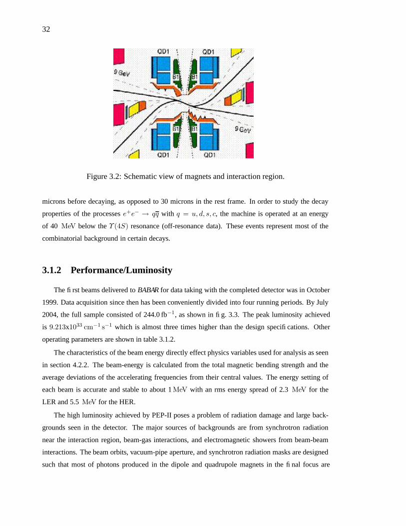
32

Figure 3.2: Schematic view of magnets and interaction region.

microns before decaying, as opposed to 30 microns in the rest frame. In order to study the decay

properties of the processes e+e− → qq with q = u, d, s, c, the machine is operated at an energy

of 40 MeV below the Υ (4S) resonance (off-resonance data). These events represent most of the

combinatorial background in certain decays.

3.1.2 Performance/Luminosity

The first beams delivered to BABAR for data taking with the completed detector was in October

1999. Data acquisition since then has been conveniently divided into four running periods. By July

2004, the full sample consisted of 244.0 fb−1, as shown in fig. 3.3. The peak luminosity achieved

is 9.213x1033 cm−1 s−1 which is almost three times higher than the design specifications. Other

operating parameters are shown in table 3.1.2.

The characteristics of the beam energy directly effect physics variables used for analysis as seen

in section 4.2.2. The beam-energy is calculated from the total magnetic bending strength and the

average deviations of the accelerating frequencies from their central values. The energy setting of

each beam is accurate and stable to about 1 MeV with an rms energy spread of 2.3 MeV for the

LER and 5.5 MeV for the HER.

The high luminosity achieved by PEP-II poses a problem of radiation damage and large back-

grounds seen in the detector. The major sources of backgrounds are from synchrotron radiation

near the interaction region, beam-gas interactions, and electromagnetic showers from beam-beam

interactions. The beam orbits, vacuum-pipe aperture, and synchrotron radiation masks are designed

such that most of photons produced in the dipole and quadrupole magnets in the final focus are

33

dumped outside the detector. Beam-gas backgrounds from bremsstrahlung and Coulomb scattering

off of gas molecules was reduced in the first year of running by scrubbing of residual absorbed

surface gasses on the vacuum surface. These types of backgrounds are the major source of radiation

to the SVT and the dominant background in most other detectors. Finally electromagnetic show-

ers from radiative Bhabha scattering are a source of background which scales with the luminosity.

Comparisons of data taken from beams in collision and beams separated show larger EMC crystal

occupancy and higher trigger rates. This increase is due to the flux of photons originating from small

angle radiative Bhabha scattering. This effect will increase with luminosity and therefore limit the

EMC energy resolution.

Table 3.1: PEP-II design and highest luminosity operating parameters. LER and HER refer

to the high energy e− and low energy e+ ring respectively. σx, σy, and σz refer to the

horizontal, vertical, and longitudinal size of the luminous region.

Parameters Design Best/typical

Energy HER/LER (GeV) 9.0/3.1 9.0/3.1

Current HER/LER (A) 0.75/2.15 2.450/1.55

Number of Bunches 1658 1588

Bunch spacing (ns) 4.2 6.3 − 10.5

σx (µm) 110 120

σy (µm) 3.3 5.6

σz (mm) 9 9

Luminosity (1033cm−2s−1) 3 9.213

Luminosity (pb−1/day) 135 710.5

3.2 Detector

The BABAR detector is made of five sub-detectors used for tracking and/or particle identifica-

tion. The tracking components of the detector operate in a 1.5 T magnetic field produced by the

super-conducting solenoid. The detector center is shifted by 37 cm with respect to the Interaction

Point (IP) in the direction of the LER to increase detection acceptance of the boosted system.

The detector is designed to have a minimum amount of material in the tracking region before

34

Nov 1

Jan 1

1999

Mar 1

May 1

Jul 1 Sep 1 N

ov 1 Jan 1

2000

Mar 1

May 1

Jul 1 Sep 1 N

ov 1 Jan 1

2001

Mar 1

May 1

Jul 1 Sep 1 N

ov 1 Jan 1

2002

Mar 1

May 1

Jul 1 Sep 1 N

ov 1 Jan 1

2003

Mar 1

May 1

Jul 1

2004

0

20

40

60

80

100

120

140

160

180

200

220

240

Inte

grat

ed L

umin

osity

(fb

-1)

BA BA R

PEP-II Delivered 253.55/fbBABAR Recorded 244.06/fb

BABAR off-peak 22.68/fb

Figure 3.3: BABAR integrated luminosity from October 1999 to July 2004.

reaching the Calorimeter to avoid multiple scattering of tracks and enhance detection of low en-

ergy photons. The Silicon Vertex Tracker (SVT) and the Drift Chamber (DCH) provide optimal

tracking capability over a wide range of momenta. The SVT is positioned close to the IP and pro-

vides excellent vertex resolution and tracking for low momentum particles. The DCH determines

the momentum of charged particles to a great precision. The next detector going radially out from

the center is the Detector of Internally Reflected Cherenkov light (DIRC) which provides particle

identification for higher momentum particles. Next is the Electromagnetic Calorimeter which mea-

sures the electromagnetic energy deposited in the crystals. Then the outermost sub-detector is the

Instrumented Flux Return (IFR) which aids in muon identification and neutral hadron detection.

Longitudinal and transverse diagrams of the detector are shown in fig. 3.4.

3.2.1 Silicon Vertex Tracker (SVT)

The SVT is designed to measure the angle and position of charged tracks to great precision.

This level of precision is defined by the need to determine the B longitudinal decay vertex position,

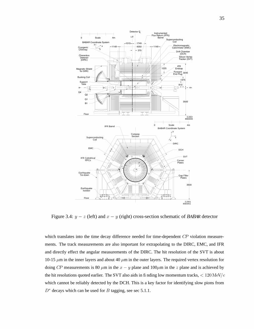
35

��

� �

��

��

��

��

��

��

��

�

��

��

�

�

�

��

Scale

BABAR Coordinate System

0 4m

Cryogenic Chimney

Magnetic Shield for DIRC

Bucking Coil

Cherenkov Detector (DIRC)

Support Tube

e– e+

Q4Q2

Q1

B1

Floor

yx

z1149 1149

Instrumented Flux Return (IFR))

BarrelSuperconducting

Coil

Electromagnetic Calorimeter (EMC)

Drift Chamber (DCH)

Silicon Vertex Tracker (SVT)

IFR Endcap

Forward End Plug

1225

810

1375

3045

3500

3-2001 8583A50

1015 1749

4050

370

I.P.

Detector CL

�

�

��

IFR Barrel

Cutaway Section

ScaleBABAR Coordinate System

y

xz

DIRC

DCH

SVT

3500

Corner Plates

Gap Filler Plates

0 4m

Superconducting Coil

EMC

IFR Cylindrical RPCs

Earthquake Tie-down

Earthquake Isolator

Floor

3-2001 8583A51

Figure 3.4: y − z (left) and x− y (right) cross-section schematic of BABAR detector

which translates into the time decay difference needed for time-dependent CP violation measure-

ments. The track measurements are also important for extrapolating to the DIRC, EMC, and IFR

and directly effect the angular measurements of the DIRC. The hit resolution of the SVT is about

10-15 µm in the inner layers and about 40 µm in the outer layers. The required vertex resolution for

doing CP measurements is 80 µm in the x− y plane and 100µm in the z plane and is achieved by

the hit resolutions quoted earlier. The SVT also aids in finding low momentum tracks, < 120MeV/c

which cannot be reliably detected by the DCH. This is a key factor for identifying slow pions from

D∗ decays which can be used for B tagging, see sec 5.1.1.

36

The design and coverage of the SVT is mostly constrained by the dipole magnets used to bring

the beams into collision. In the forward direction it covers up to 350 mrad in polar angle from

the beam line and 520 mrad in backward direction. This sub-detector is made of five layers of

340 double-sided silicon strip wafers mounted on a carbon-fiber frame. The silicon semiconductor

works basically as a reversed bias p-n junction; when a charged particle traverses the volume it

creates an electron-hole pair which under a voltage will flow to the surface where it is measured

by charge integrating contacts. The detector is separated into p-n junction strips with individual

readouts so that the path of the particle can be traced by the location of the strips which produce a

signal.

The sensors on each side of the wafers are orthogonal to each other allowing for both a z and φ

position measurement of the track and provide 150,000 channels of information. To avoid having

too much material in the acceptance region, which causes scattering, the readout electronics are all

housed in the backward region of the SVT, outside the fiducial volume. The inner three layers are

placed close to the beam-pipe to determine position and angle of the B vertex while the outer two

are placed closer to the DCH for extrapolating tracks into the DCH. Fig. 3.5 shows the longitudinal

and transverse schematic drawings of the SVT.

3.2.2 Drift Chamber (DCH)

The main purpose of the DCH is to determine the momentum of charged particles in the plane

transverse to the beam. A particle must have a minimum transverse momentum of 50 MeV to reach

the DCH and a momentum of about 120 MeV to be reliably reconstructed. The DCH measures

280 cm long and occupies the radial volume from 23.6 to 80.9 cm. This area is filled with a 80:20

mixture of helium and isobutane gas at 4 mbar above the atmospheric pressure. Charged particles

traveling in the DCH ionize the gas thereby creating electrons which drift along field lines to sense

wires at the center of each drift chamber cell. Near the sense wire, the electron causes an avalanche

in the locally high field gradient, resulting in a detectable signal that can be used to measure the

drift time. With the help of a time-to-distance relation one can relate the drift time to the distance

away from the wire in a given cell.

The DCH is made of 40 layers of 7104 hexagonal shaped cells of about 1 cm width. Each cell

contains a sense wire surrounded by six field wires, see fig 3.6. The aluminum field wires are held

at a ground potential while the tungsten-rhenium sense wires are held at a positive high voltage of

1930 V.1

1DCH operated at voltage of 1960V from , a voltage of 1900 V from, and a voltage of 1930 V from tillpresent.

37

Beam Pipe 27.8mm radius

Layer 5a

Layer 5b

Layer 4b

Layer 4a

Layer 3

Layer 2

Layer 1

580 mm

350 mrad520 mrad

ee +-

Beam Pipe

Space Frame

Fwd. support cone

Bkwd. support cone

Front end electronics

Figure 3.5: x− (left) and y − z (right) cross-section schematic of BABAR SVT.

The layers of the DCH are organized in subsets of 4 layers, or 10 superlayers. Four of the ten

superlayers are axial layers where the wires run parallel to the axis of the chamber and the remaining

six are stereo layers where they are rotated by some angle. The stereo superlayers alternate in stereo

angle rotation to allow a determination of the z-coordinate of the tracks. The axial layers determine

the φ-coordinate of the track.

At low momentum the DCH energy loss per unit distance can be used for particle identification.

The transverse momentum resolution of the track is given by:

σpT = (0.13 ± 0.01)%pT + (0.45 ± 0.03)% (3.1)

3.2.3 Detector of Internally Reflected Cherenkov Light (DIRC)

The DIRC is perhaps the most innovative sub-detector providing particle identification at high

momentum by measuring Cherenkov radiation from particles traveling through synthetic fused silica

bars. The DIRC is used for separating kaons and pions which is useful for flavor identification in

38

0Stereo

1 Layer

0Stereo

1 Layer

0 2 0 2 0 2

0 3

0 4 0 4

45 5 45 5

47 6 47 6 47 6

48 7 48 7

50 8

-52 9

-5410

-5511

-5712

013 013

014 014

015

016

4 cm

Sense Field Guard Clearing

1-2001 8583A14

Figure 3.6: Schematic layout of DCH cells for the four inner superlayers. The numbers on

the right indicate the stereo angle for each layer.

cascade processes like b → c → s. It is also used for separating two-body charmless decays to

pions and kaons to great precision. The DIRC can measure photon arrival time to an accuracy of

1.7 ns, which allows it to distinguish signal and background in a high luminosity environment.

The 1444 9m × 1.7 cm × 3.5 cm silica bars are arranged into a 12-sided polygonal barrel. The

light produced is transmitted through total internal reflection to the array of photomultiplier tubes

at the backward end of the magnet (see fig. 3.7). Before reaching the PMT, the light passes through

a water filled standoff box and produces rings of light in the shape of cones. The opening angle of

the cone is the Cherenkov production angle modified by refraction at the end of fused silica bars.

Upon exiting the bars the photons are focused on the PMT through the aperture of the bar which

acts as a pinhole source. The vector pointing from the center of the bar end to the center of each

PMT is taken as the photon propagation angle. Together with the polar angle measured from the

tracking system which can be associated with the photon transversing the bar one can determine

the Cherenkov angles. The timing info from the PMTs provides an extra constraint on the system

which can help in identifying backgrounds and ambiguous signal.

The DIRC has a K − π separation power of 4σ at 3 GeV, but for tracks of order 0.7 GeV the

39

Mirror

4.9 m

4 x 1.225m Bars glued end-to-end

Purified Water

Wedge

Track Trajectory

17.25 mm Thickness (35.00 mm Width)

Bar Box

PMT + Base 10,752 PMT's

Light Catcher

PMT Surface

Window

Standoff Box

Bar

{ {1.17 m

8-2000 8524A6

Figure 3.7: Schematic drawing illustrating the detection of Cherenkov photons by the

DIRC.

SVT and DCH dE/dx is used for particle identification. The average resolution on the Cherenkov

angle is 2.5 mrad and the timing resolution is such that photons from different beam crossings are

distinguished as separate events.

3.2.4 Electromagnetic Calorimeter (EMC)

The EMC is designed to measure electromagnetic showers with excellent resolution in angle

and energy for particles ranging in energy from 20 MeV to 9 GeV. This allows for detection of

photons from π0 or η0 decays, and electromagnetic and radiative processes. Lepton identification

aids in flavor tagging of neutral B decays. QED processes like e +e− → e+e−γ and e+e− → γγ

are used for calibrations and luminosity determinations. At the low energy detection scale is set

by the need to reconstruct π0 or η0 from B decays. Below energies of 2 GeV π0 reconstruction is

dominated by energy resolution, 1-2%, and at higher energies by the angular resolution.

The EMC is made of 6,580 Cesium-Iodide crystals doped with a small amount of Thalium.

Most of the crystals cover the barrel region of the detector in φ, (see fig 3.8), and about 10% are

in the forward end-cap region, the direction of the boost to achieve larger acceptance. The EMC

is more than 96% efficient for photons with energy greater than 20 MeV. The energy resolution is

given byσ(E)

E=

2.32 ± 0.30)%

E1/4± (1.85 ± 0.12)%. (3.2)

40

The angular resolution is determined from the reconstruction of π0 and η0, which decay into two

photons, and is

σ(φ) = σ(θ) =3.87 ± 0.07)%

E(GeV)1/2± (0.00 ± 0.04)mrad. (3.3)

11271375920

1555 2295

2359

1801

558

1979

22.7˚

26.8˚

15.8˚

Interaction Point 1-2001 8572A03

38.2˚

External Support

Figure 3.8: Schematic drawing of top half of EMC in y-z. Dimensions are in mm.

3.2.5 Internal Flux Return (IFR)

The IFR is used for muon and neutral hadron identification over a wide range of angles and

momenta. The detection of muons is essential for determining the flavor of a B decaying semilep-

tonically. The relative fraction of muon tags to all other flavor tagged channels is about 6%. This

lepton channel suffers from a much lower flavor identification uncertainty, however, making the rel-

ative effective efficiency about twice as high, (see sec. 5.1.3). K0L detection allows for reconstruction

of B meson decays in additional CP eigenstates.

The IFR is instrumented with 806 Resistive Plate Chambers (RPC) placed between the steel

plates that make up the magnet flux return for the detector. The RPCs are sandwiched between

layers of steel increasing from thickness from 2 cm in the inside to 10 cm on the outside. There

are 19 layers of RPCs in the barrel section and 18 layers in the end caps (see fig. 3.9).

Muons with at least 1 GeV of energy travel through the RPCs where they are detected by limited

streamer discharge. Particles are identified as muons if they have a long penetration distance in the

iron. A K0L produces a larger cluster in the RPCs when it interacts in the iron, with the additional

signature of having no track leading to the energy deposition.

41

Barrel 342 RPC Modules

432 RPC Modules End Doors

19 Layers

18 LayersBW

FW

3200

3200

920

12501940

4-2001 8583A3

Figure 3.9: Schematic drawing of IFR barrel and endcap.

3.2.6 Trigger

There are two levels of trigger used on the BABAR experiment. The first, Level 1 trigger, is a

hardware trigger operating at 2 kHz during normal running. The second is a software trigger Level

3 operating at ∼ 200 Hz for physics and ∼ 100 Hz for other special event categories. The trigger

is used to reject the uninteresting events and accept the ones which would be of physics interest in

an efficient and unbiased method while keeping the total event rate under 120 Hz. The rates for

the Level 1 trigger for events of interest are shown in table 3.2. The Level 1 trigger operates on a

11-12 µs latency with respect to the e+e− collisions and delivers triggers to the Fast Control and

Timing System (FCTS). The Level 1 accept algorithm is based on charged track candidates in the

DCH, showers in the EMC, and tracks in the IFR. The hardware for the Level 1 trigger is stored in

several VME crates associated with each subsystem. Once a valid trigger remains a Level 1 accept

is issued and events are read out and sent to the software Level 3 trigger. The Level 1 trigger takes

approximately 1 µs to receive the accept from the FCTS and initiate readout from the Read Out

Modules (ROM).

The Level 3 trigger runs on the assembled events, and so can use sophisticated algorithms

based on complete events to reduce background and keep interesting events. The software runs

on commercial machines (nodes) which run the Online Processing Software (OEP) which partially

reconstructs the event in order to apply the Level 3 trigger and also provide plots for monitoring

data to people on shift.

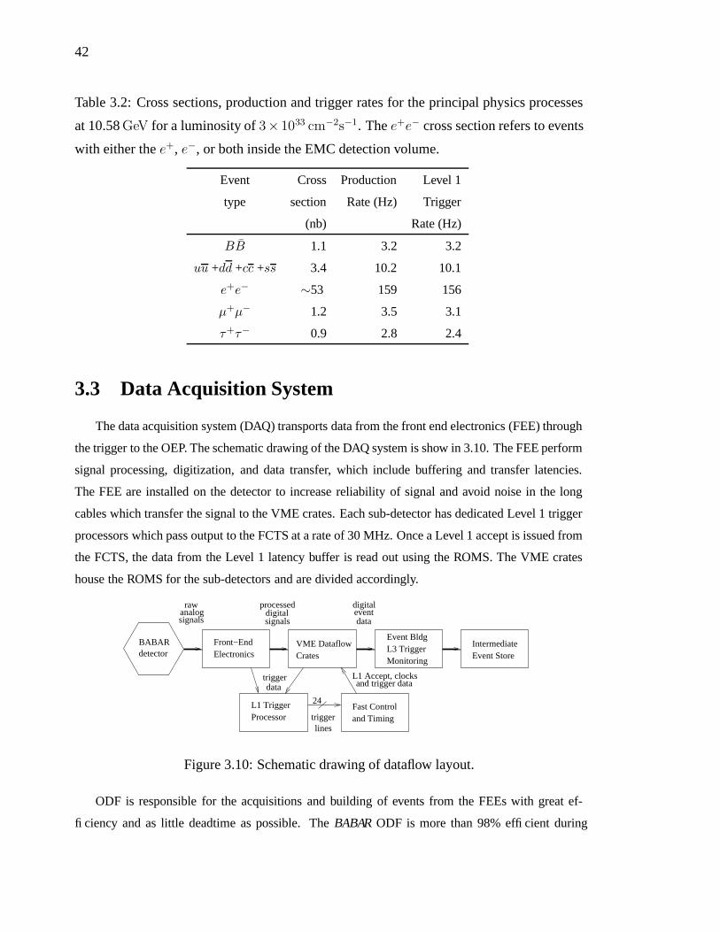
42

Table 3.2: Cross sections, production and trigger rates for the principal physics processes

at 10.58 GeV for a luminosity of 3× 1033 cm−2s−1. The e+e− cross section refers to events

with either the e+, e−, or both inside the EMC detection volume.

Event Cross Production Level 1

type section Rate (Hz) Trigger

(nb) Rate (Hz)

BB 1.1 3.2 3.2

uu +dd +cc +ss 3.4 10.2 10.1

e+e− ∼53 159 156

µ+µ− 1.2 3.5 3.1

τ+τ− 0.9 2.8 2.4

3.3 Data Acquisition System

The data acquisition system (DAQ) transports data from the front end electronics (FEE) through

the trigger to the OEP. The schematic drawing of the DAQ system is show in 3.10. The FEE perform

signal processing, digitization, and data transfer, which include buffering and transfer latencies.

The FEE are installed on the detector to increase reliability of signal and avoid noise in the long

cables which transfer the signal to the VME crates. Each sub-detector has dedicated Level 1 trigger

processors which pass output to the FCTS at a rate of 30 MHz. Once a Level 1 accept is issued from

the FCTS, the data from the Level 1 latency buffer is read out using the ROMS. The VME crates

house the ROMS for the sub-detectors and are divided accordingly.

Front−EndElectronics

VME DataflowCrates

L1 TriggerProcessor

Fast Controland Timing

Event BldgL3 TriggerMonitoring

IntermediateEvent Store

dataeventdigitalraw

signalsanalog

signals

processeddigital

data

BABARdetector

trigger

24

L1 Accept, clocksand trigger data

linestrigger

Figure 3.10: Schematic drawing of dataflow layout.

ODF is responsible for the acquisitions and building of events from the FEEs with great ef-

ficiency and as little deadtime as possible. The BABAR ODF is more than 98% efficient during

43

normal running. ODF builds events by harvesting data from each crate into another set of ROMS

which are connected to the online nodes (farm) via an Ethernet network. After passing through the

Level 3 trigger which is described above, the data is passed onto the online prompt reconstruction

(OPR). OPR is responsible for an more extensive monitoring system and selection of physics events.

Rolling calibrations which involve applying constants calculated from one run to a future run are

also done on OPR. These constants and the events reconstructed at OPR are stored in the conditions

database and the object oriented event store. This data is accessible to users for running analysis

programs.

3.3.1 Online Detector Control and Run Control

During data taking there are personnel on shift monitoring the detector and the plots provided

by the OEP to insure all elements of the detector and the DAQ system are working properly. The

Online Detector Control (ODC) system controls and monitors the detector through the use of EPICS,

Experimental Physics and Industrial Control System. Through the EPICS controls one can monitor,

diagnose, and control the detector. EPICS also provides alarms in case of problems from the detector

and has an interface to PEP-II and the magnet controls. The online run control (ORC) allows for

operation of the DAQ system. One can take out certain VME crates during running, configure the

ROMS, start up OEP, and begin, pause, or end runs. Calibrations of the subsystems can also be

done using ORC. All this functionality is stored into one graphical interface at IR2.

3.4 Candidate Reconstruction

The particles which are identified by the detector are pions, electrons, muons, kaons, protons,

photons, and K0L mesons. All other particles are made of some combination of those on this list.

Charged particles have an associated track which can be identified by the SVT and DCH. Neutral

particles will only leave a signature in the EMC and IFR. Photons are detected by the EMC and

muons and K0L mesons by the IFR. The difference between a kaon and pion is determined by the

SVT and DCH dE/dx for lower energies and for higher energies by the DIRC. The next two sections

describe track reconstruction and particle identification in the detector.

3.4.1 Track Reconstruction

The reconstruction of charged tracks relies on information from the SVT and DCH. There are

five parameters describing the helical shape of the track in the detector. These parameters are d0, φ0,

44

ω, z0, and tanλ; see fig 3.11 for a graphical representation of the variables. d0 and z0 are measured

at the point of closest approach to the z axis and are defined as the distance in x − y to this point

and the distance in z to this point respectively. φ0 and λ are the azimuth angle and dip angle with

respect to x− y respectively. And finally ω is the curvature and is defined as 1/pT . ω and d0 carry

signs which are related to the sign of the particle.

The track finding algorithm starts with information from the trigger system. The Level 1 trig-

ger recognizes tracks as four contiguous track segments (hits) in two dimensions. Then the Level

3 trigger software goes one step further with DCH hit pattern recognition which provides the first

estimate of d0, φ0, and the event start time t0. After passing several other offline track finder algo-

rithms in the DCH, the tracks are fit with a Kalman-Filter fitter which takes into account material

interactions, energy loss, and non-uniformity of the magnetic field in the detector. One of the DCH

algorithms is designed to find long-lived particles, such as the K0S meson, which may not leave hits

in the SVT.

The fitted DCH track is then extrapolated into the SVT and SVT track segments are added. The

SVT segment with the smallest residuals and largest number of SVT hits is used to connect to the

DCH track. Again a Kalman fit is performed to the whole SVT-DCH track to obtain a more refined

fit to the track. Any remaining SVT hits are used in two separate algorithms to search for tracks.

One of the algorithms searches for spatially dispersed hits in z0 and d0 and the other for hits which

are confined to a small area in z. Finally the algorithms try to match SVT and DCH tracks which

could have discontinuities due to scattering.

Track reconstruction resolution is determined with cosmic ray events by comparing fits to cos-

mic track halves in the upper and lower region of the detector. The resolutions for particles with

energy > 3GeV are σd0 = 23µm, σφ0 = 0.43 mrad, σz0 = 29µm, and σtanλ= 0.53 x10−3. The

pT resolution as a function of pT is also shown in fig 3.12.

3.4.2 Particle Identification (PID)

As noted in section 3.4 there are a few long-lived particles which leave signals in detector

systems. In general, among these long-lived objects, we need to differentiate between kaons and

pions, differentiate energy deposits in the EMC from photons or charged tracks, and identify muons

and K0L mesons from the IFR. Particle identification is a key ingredient for determining the flavor

of the B mesons as described in 5.1.

For charged particles with momenta below about 0.7 GeV/c, the the SVT and DCH dE/dx is

used for PID. The 80% truncated mean dE/dx in the DCH is used to compute likelihoods for pions,

45

Y

Z(0,0)

z0

Point of closestapproach in (x,y)

λθ

e- 9 GeV e+ 3 GeV

B

X

Y

L

e+

r

d0

d_

B_

t_

φ

X

Y

Z

Figure 3.11: Track parameters shown in y-z coordinates (top) and x-y coordinates (bottom).

kaons, and protons assuming a Gaussian error around the nominal Bethe-Block expectation for the

known momentum. The distribution of dE/dx in the DCH as a function of momentum is shown

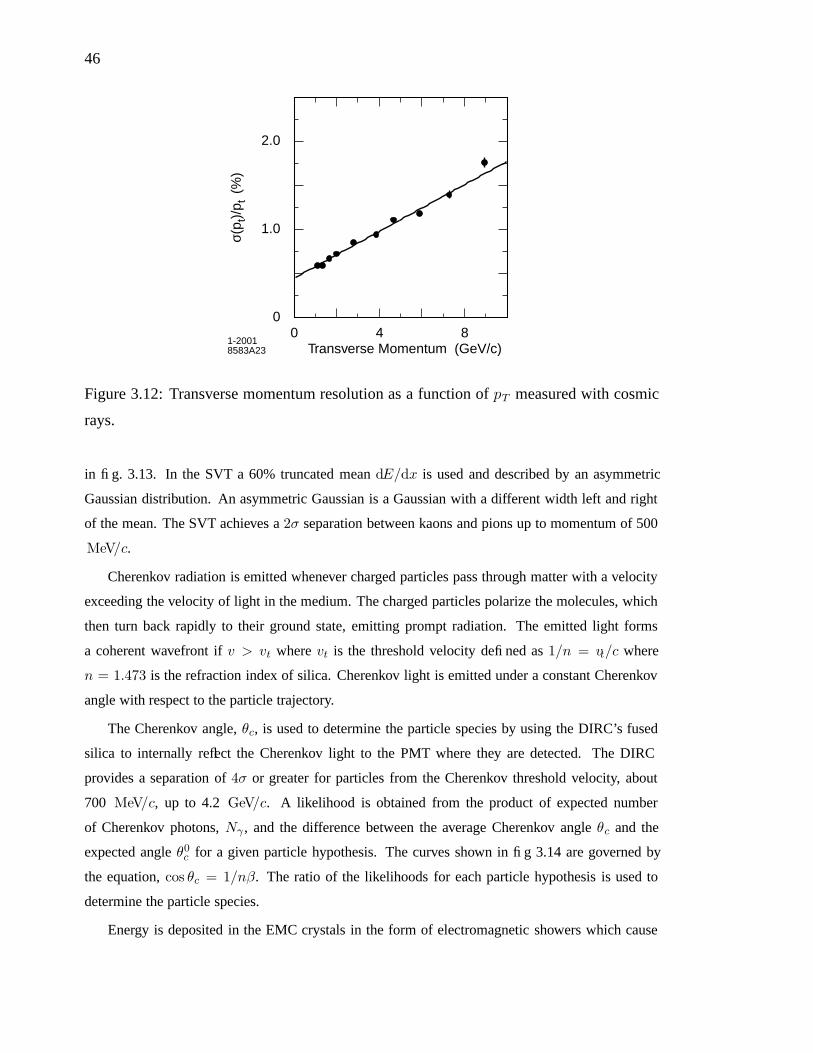
46

0

1.0

2.0

0 4 8Transverse Momentum (GeV/c)

σ(p t

)/p t

(%

)

1-2001 8583A23

Figure 3.12: Transverse momentum resolution as a function of pT measured with cosmic

rays.

in fig. 3.13. In the SVT a 60% truncated mean dE/dx is used and described by an asymmetric

Gaussian distribution. An asymmetric Gaussian is a Gaussian with a different width left and right

of the mean. The SVT achieves a 2σ separation between kaons and pions up to momentum of 500

MeV/c.

Cherenkov radiation is emitted whenever charged particles pass through matter with a velocity

exceeding the velocity of light in the medium. The charged particles polarize the molecules, which

then turn back rapidly to their ground state, emitting prompt radiation. The emitted light forms

a coherent wavefront if v > vt where vt is the threshold velocity defined as 1/n = vt/c where

n = 1.473 is the refraction index of silica. Cherenkov light is emitted under a constant Cherenkov

angle with respect to the particle trajectory.

The Cherenkov angle, θc, is used to determine the particle species by using the DIRC’s fused

silica to internally reflect the Cherenkov light to the PMT where they are detected. The DIRC

provides a separation of 4σ or greater for particles from the Cherenkov threshold velocity, about

700 MeV/c, up to 4.2 GeV/c. A likelihood is obtained from the product of expected number

of Cherenkov photons, Nγ , and the difference between the average Cherenkov angle θc and the

expected angle θ0c for a given particle hypothesis. The curves shown in fig 3.14 are governed by

the equation, cos θc = 1/nβ. The ratio of the likelihoods for each particle hypothesis is used to

determine the particle species.

Energy is deposited in the EMC crystals in the form of electromagnetic showers which cause

47

104��

103��

10–1 101

eµ

π

K

pd

dE/d

x

Momentum (GeV/c)1-2001 8583A20

Figure 3.13: DCH dE/dx as a function of track momenta. The solid curves are the Bethe-

Bloch expectations for different long-lived particle species.

p GeV/c

θ c ra

dian

s

B A B A R

πK

0.775

0.8

0.825

0.85

2 3 4 5

Figure 3.14: The measured Cherenkov opening angle θc for kaons and pions versus mo-

mentum.

energy deposition in clusters of many adjacent crystals. Photons from high momentum π0 and η0

decays can produce two energy maxima (bumps) within a cluster due to the small opening angle.

The EMC reconstruction algorithm starts with crystals with an energy deposit > 10MeV and adds

energies from adjacent crystals until a bump is built. A bump is associated with a charged track if

48

the projection from the bump onto the inner face of the EMC is consistent with a extrapolated track

trajectory. Otherwise the bump is associated with a neutral particle with a trajectory originating at

the interaction point.

The photon energy scale is calibrated with a radioactive source at low energies, with e+e−

Bhabha scattering events at high energies, and with decays of π0 and η mesons at energies below

2 GeV (fig. 3.15). The ratio of energy E deposited in the EMC to the track momentum p, E/p, is

equal to one for electrons in an ideal calorimeter. The E/p distribution for electrons is shown in

fig. 3.16. The distribution peaks at E/p slightly less than unity due to shower leakage and other

resolution effects.

(GeV)γγ

m0.05 0.1 0.15 0.2 0.25

En

trie

s /

0.0

01

Ge

V

0

2000

4000

6000

8000

10000

12000

mass = 135.1 MeV0π

width = 6.9 MeV0π

(a)

measured energy / expected deposited energy0.6 0.7 0.8 0.9 1 1.1 1.2 1.30

500

1000

1500

2000

2500

3000 (b)

Figure 3.15: (a) π0 mass distribution constructed from two photon candidates in hadronic

events (histogram) overlaid with a fit (curve). (b) Ratio of measured to expected energy for

electrons in Bhabha events (histogram) overlaid with a fit (curve).

Muons are identified by comparing the expected interaction length, λexp and the measured λ.

Other variables such as the average multiplicity of hit strips per layer and it standard deviation, the

χ2 of the track, and the continuity of the tracks Tc, help reject contamination from hadronic showers.

Hadrons can interact in the material and therefore lead to a broader distribution of hits, hence a larger

χ2. Muons on the other hand will match the track extrapolation into the IFR reasonably well.

The muon efficiency for particles with momentum > 1.5GeV is about 60% with a pion fake

rate of < 2.5%. The muon efficiency at BABAR has been degrading at a rate of 1% per month. This

decrease is due to the contamination of linseed oil used to coat the RPC chambers. The contam-

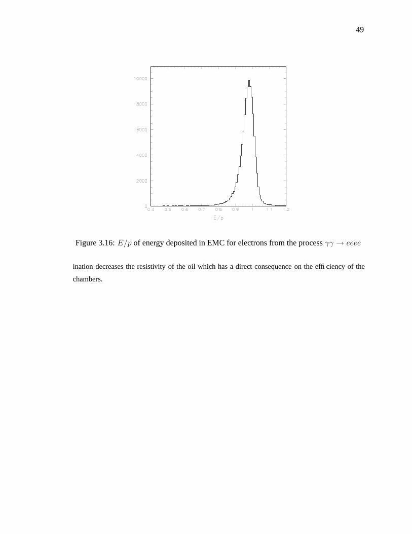
49

Figure 3.16: E/p of energy deposited in EMC for electrons from the process γγ → eeee

ination decreases the resistivity of the oil which has a direct consequence on the efficiency of the

chambers.

Chapter 4

Event Reconstruction and Fitting

Technique

In this chapter we will discuss and define the variables needed to select the events which will be

used in the time-dependent CP analysis. Chapter 5 is reserved for discussion of the time components

of the decay while this chapter focuses on the reconstruction and selection of events. At the end of

the chapter we will discuss the method for extracting information from the maximum likelihood fit

and define Toy MC samples.

Once the data is processed at OPR as discussed in sec. 3.3, it is stored in the event store database

for use in analysis. A series of very loose selection requirements similar to analysis code only less

specialized are used in OPR to separate out events of interest to certain groups. These lists are

called skims and are stored in the database and labeled for the specific mode of reconstruction.

This analysis uses the BKsKsKs3body skim which selects only 0.01% of the total events. Having

the skims makes it much faster and requires fewer computing resources to run more complicated

analysis code over the small sample of interest.

From the skims one can run analysis software which takes the list ofK 0S candidates in the events

and applies combinatorics and vertexing code with some loose kinematic selections. From here a

set of analysis ntuples are made which can be used for modifying and fine tuning the final selection

requirements for the analysis. For this analysis, the same set of signal-to-background optimized

requirements are made as for the branching fraction measurement [22].

Once the final selection requirements are made another set of smaller ntuples are made with

corresponding datasets and ascii files for use in the maximum likelihood fit to extract the CP asym-

metries. The maximum likelihood fit is done in a fitting package which interfaces to RooFit, a fitting

50

51

package used in high energy physics experiments [23]. From the small set of ntuples one can use

the data sidebands (see sec. 4.2.2) to parametrize the backgrounds events. The signal MC events are

used for parameterizing the signal events.

A fit with no ∆t information is made to determine the approximate yields expected from the

sample for the purpose of generating Toy MC events as described in sec. 4.5. Once tests are done

with the Toy MC events to show the fit is unbiased one can perform a blind fit to compare the

uncertainties on the asymmetries with the Toy MC expectations. The analysis is done blind meaning

that the actual value of the asymmetries are hidden in order to avoid any bias from the experimenter.

Once all validations are performed and the fit is determined to be unbiased, we can unblind the

result.

We’ve only touched briefly on the time-dependent part of the analysis in this overview. We will

discuss vertexing and determining ∆t in greater detail in chapter 5.

4.1 Event Samples

The samples used for this analysis are on and off resonant data and signal MC. The signal MC

are divided into SP5 and SP6 which correspond to conditions in runs 1-3 and run 4 respectively.

• Data: Run 1-4 on-resonance data corresponding to 205 fb−1.

• Data: Run 1-4 off-resonance data corresponding to 16 fb−1.

• MC: SP5 B0 → K0SK

0SK

0S 120K K0

S → π+π− and π0 π0

• MC: SP6 B0 → K0SK

0SK

0S 200K K0

S → π+π− only

• MC: B0B0 269,590K ≈ 513 fb−1

• MC: B+B− 280,030K ≈ 533 fb−1

4.2 Event Selection

There are several physics events which occur at the B factory. Some of these events are back-

ground events which need to be removed. Other event types are used for calibrations and luminosity

studies. The Υ (4S) decays are of course of interest for our analysis and therefore need to be selected

from the whole set of physics events. It is therefore useful to distinguish the different set of events

which can be used for various studies. Table 4.2 lists the various event types.

52

Physics events can be distinguished into different types through the use of two discriminating

variables: the visible energy W and the event topology R2 which will be discussed in this section.

Events with Υ (4S) → BB decays will have a large number of hadrons and an isotropic topol-

ogy since the left over energy from the decay is small. Continuum physics events will have dis-

tinguishing traits like having jet-like topology from the hadronization of quarks produced back-to-

back. Other decays, like e+e− → γγ will have large missing energy and a small number of tracks.

So in general by monitoring the visible energy, the event topology, and the track multiplicity we are

able to distinguish between different physics events. Table 4.2 shows the characteristics of different

physics results.

Table 4.1: Main characteristics of the physics processes at the Υ (4S) energy, in the center-

of-mass frame.

Event type Topology Visible Energy Number of Tracks

e+e− → e+e− Back-to-Back Deposit in EMC 2 high momentum

e+e− → µ+µ− Back-to-Back Visible 2 high momentum

e+e− → τ+τ− Back-to-Back large missing en-

ergy from neutri-

nos from semilep-

tonic decays

2 leptons

e+e− → γγ large missing en-

ergy

small number of

tracks

e+e− → qq with

q = u, d, s, c

jet-like from

hadronization of

quarks produced

back-to-back

mean of 6 GeV large

e+e− → Υ (4S) →BB

Isoptropic mean of 6 GeV large

The visible energy W is defined as the sum over all charged and neutral tracks in the tracking

fiducial area,

W =

charged∑

i

√

m2π + p2

i +neutral∑

j

Ej . (4.1)

53

The distribution of the number of charged tracks and W are shown in figures 4.1 and 4.2 respectively

for MC events. We remove QED events by selecting events with at least three charged tracks and a

total visible energy greater than 4.5GeV.

bb−

qq− continuum

τ+τ-

µ+µ-(γ)

e+e-(γ)

γγ

Number of tracks

Arb

itrar

y un

its

0

0.05

0.1

0.15

0.2

0.25

0.3

0 2 4 6 8 10 12 14 16

Figure 4.1: MC distribution of the number of charged tracks in the fiducial area in the main

physics processes at the Υ (4S) energy. The distributions are normalized to the same area,

rather then the relative rate..

To further discriminate from continuum uu, dd, ss, and cc events we use a variable R2 that

is sensitive to the overall event topology. R2 is defined as the ratio of the second to zeroth order

Fox-Wolfram moments Hl

Hl =∑

i,j

|pi||pj|E2T

Pl(cosθij), (4.2)

where Pl are the Legendre polynomials, pi are the particle momenta, θi,j is the angle between the

particles i and j, and ET is the total energy in the event. The distribution of R2 ≡ H2/H0 for

different physics events is shown in fig 4.3.

4.2.1 Reconstruction of K0S→ π+π−

K0S candidates are reconstructed in the decay mode π+π− which has a branching fraction of

68.95% [13]. A pair of charged track candidates are required to originate from the same point in

space (vertex fit). Candidates with an invariant mass of |MK0S−MPDG

K0S

| < 12MeV are selected,

whereMPDGK0

S

= 497.6MeV [13]. The invariant mass m(π+ π−) of the selected candidates is shown

in fig. 4.4. Other selection requirements made on the K0S candidate are:

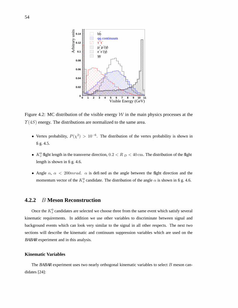
54

bb−

qq− continuum

τ+τ-

µ+µ-(γ)e+e-(γ)γγ

Visible Energy (GeV)

Arb

itrar

y un

its

0

0.02

0.04

0.06

0.08

0.1

0.12

0.14

0 1 2 3 4 5 6 7 8 9 10 11

Figure 4.2: MC distribution of the visible energy W in the main physics processes at the

Υ (4S) energy. The distributions are normalized to the same area.

• Vertex probability, P (χ2) > 10−6. The distribution of the vertex probability is shown in

fig. 4.5.

• K0S flight length in the transverse direction, 0.2 < R D < 40 cm. The distribution of the flight

length is shown in fig. 4.6.

• Angle α, α < 200mrad. α is defined as the angle between the flight direction and the

momentum vector of the K0S candidate. The distribution of the angle α is shown in fig. 4.6.

4.2.2 B Meson Reconstruction

Once the K0S candidates are selected we choose three from the same event which satisfy several

kinematic requirements. In addition we use other variables to discriminate between signal and

background events which can look very similar to the signal in all other respects. The next two

sections will describe the kinematic and continuum suppression variables which are used on the

BABAR experiment and in this analysis.

Kinematic Variables

The BABAR experiment uses two nearly orthogonal kinematic variables to select B meson can-

didates [24]:

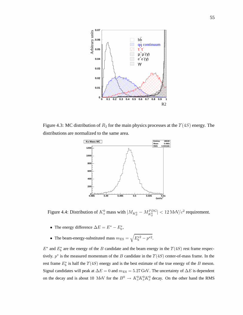
55

bb−

qq- continuum

τ+τ-

µ+µ-(γ)e+e-(γ)γγ

R2

Arb

itrar

y un

its0

0.01

0.02

0.03

0.04

0.05

0.06

0.07

0 0.1 0.2 0.3 0.4 0.5 0.6 0.7 0.8 0.9 1

Figure 4.3: MC distribution of R2 for the main physics processes at the Υ (4S) energy. The

distributions are normalized to the same area.

2GeV/c0.485 0.49 0.495 0.5 0.505 0.510

200

400

600

800

1000

1200

Ks Mass MC Entries 28539Mean 0.4981RMS 0.003166

Ks Mass MC

Figure 4.4: Distribution of K0S

mass with |MK0S−MPDG

K0S

| < 12 MeV/c2 requirement.

• The energy difference ∆E = E∗ −E∗b ,

• The beam-energy-substituted mass mES =√

E∗2b − p∗2.

E∗ and E∗b are the energy of the B candidate and the beam energy in the Υ (4S) rest frame respec-

tively. p∗ is the measured momentum of the B candidate in the Υ (4S) center-of-mass frame. In the

rest frame E∗b is half the Υ (4S) energy and is the best estimate of the true energy of the B meson.

Signal candidates will peak at ∆E = 0 and mES = 5.27GeV. The uncertainty of ∆E is dependent

on the decay and is about 10 MeV for the B0 → K0SK

0SK

0S decay. On the other hand the RMS

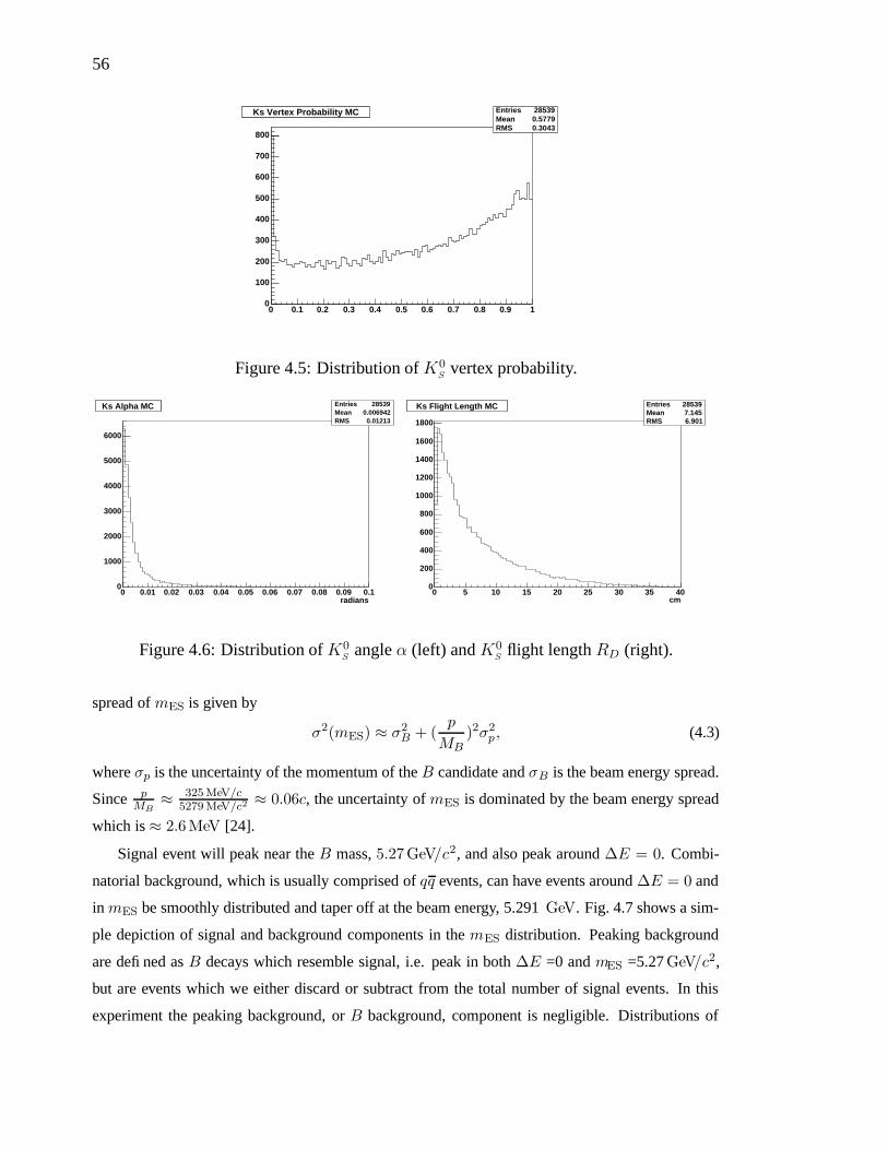
56

0 0.1 0.2 0.3 0.4 0.5 0.6 0.7 0.8 0.9 10

100

200

300

400

500

600

700

800

Ks Vertex Probability MC Entries 28539Mean 0.5779RMS 0.3043

Ks Vertex Probability MC


vertex probability.

radians0 0.01 0.02 0.03 0.04 0.05 0.06 0.07 0.08 0.09 0.1

0

1000

2000

3000

4000

5000

6000

Ks Alpha MC Entries 28539Mean 0.006942RMS 0.01213

Ks Alpha MC

cm0 5 10 15 20 25 30 35 40

0

200

400

600

800

1000

1200

1400

1600

1800

Ks Flight Length MC Entries 28539Mean 7.145RMS 6.901

Ks Flight Length MC


angle α (left) and K0S

flight length RD (right).

spread of mES is given by

σ2(mES) ≈ σ2B + (

p

MB)2σ2

p, (4.3)

where σp is the uncertainty of the momentum of the B candidate and σB is the beam energy spread.

Since pMB

≈ 325 MeV/c5279 MeV/c2

≈ 0.06c, the uncertainty of mES is dominated by the beam energy spread

which is ≈ 2.6MeV [24].

Signal event will peak near the B mass, 5.27GeV/c2, and also peak around ∆E = 0. Combi-

natorial background, which is usually comprised of qq events, can have events around ∆E = 0 and

in mES be smoothly distributed and taper off at the beam energy, 5.291 GeV. Fig. 4.7 shows a sim-

ple depiction of signal and background components in the mES distribution. Peaking background

are defined as B decays which resemble signal, i.e. peak in both ∆E =0 and mES =5.27 GeV/c2,

but are events which we either discard or subtract from the total number of signal events. In this

experiment the peaking background, or B background, component is negligible. Distributions of

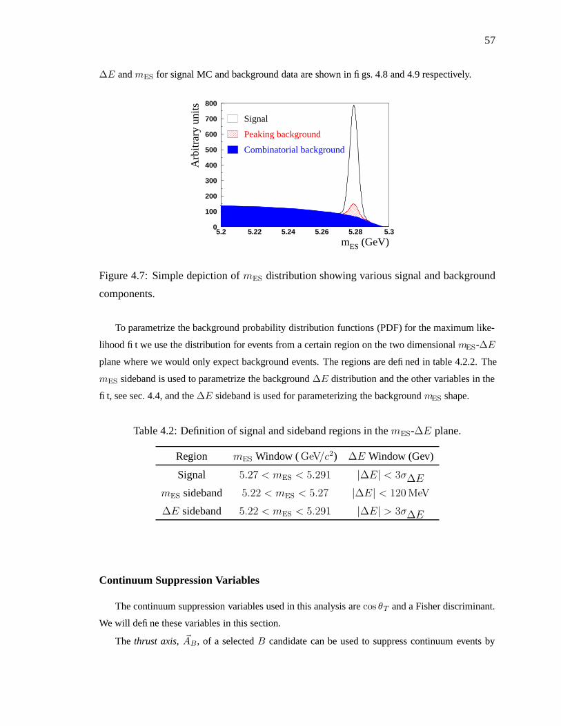
57

∆E and mES for signal MC and background data are shown in figs. 4.8 and 4.9 respectively.

Signal

Peaking background

Combinatorial background

mES (GeV)

Arb

itrar

y un

its

0

100

200

300

400

500

600

700

800

5.2 5.22 5.24 5.26 5.28 5.3

Figure 4.7: Simple depiction of mES distribution showing various signal and background

components.

To parametrize the background probability distribution functions (PDF) for the maximum like-

lihood fit we use the distribution for events from a certain region on the two dimensional mES-∆E

plane where we would only expect background events. The regions are defined in table 4.2.2. The

mES sideband is used to parametrize the background ∆E distribution and the other variables in the

fit, see sec. 4.4, and the ∆E sideband is used for parameterizing the background mES shape.

Table 4.2: Definition of signal and sideband regions in the mES-∆E plane.

Region mES Window ( GeV/c2) ∆E Window (Gev)

Signal 5.27 < mES < 5.291 |∆E| < 3σ∆E

mES sideband 5.22 < mES < 5.27 |∆E| < 120 MeV

∆E sideband 5.22 < mES < 5.291 |∆E| > 3σ∆E

Continuum Suppression Variables

The continuum suppression variables used in this analysis are cos θT and a Fisher discriminant.

We will define these variables in this section.

The thrust axis, ~AB , of a selected B candidate can be used to suppress continuum events by

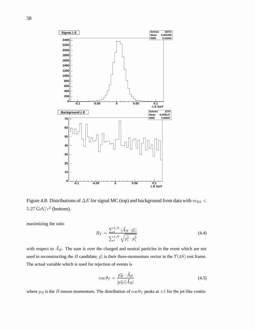
58

E GeV∆ -0.1 -0.05 0 0.05 0.1

0

200

400

600

800

1000

1200

1400

1600

1800

2000

2200

2400

E∆Signal Entries 18472Mean 0.005499RMS 0.01844

E∆Signal

E GeV∆ -0.1 -0.05 0 0.05 0.1

0

10

20

30

40

50

60

70

E∆Background Entries 2270Mean -0.008127RMS 0.06947

E∆Background

Figure 4.8: Distributions of ∆E for signal MC (top) and background from data withmES <

5.27 GeV/c2 (bottom).

maximizing the ratio

RT =

∑1,Ni | ~AB · ~pi|

∑1,Ni

√

~p∗i · ~p∗i(4.4)

with respect to ~AB . The sum is over the charged and neutral particles in the event which are not

used in reconstructing the B candidate; ~pi is their three-momentum vector in the Υ (4S) rest frame.

The actual variable which is used for rejection of events is

cos θT =~pB · ~AB| ~pB || ~AB |

(4.5)

where pB is the B meson momentum. The distribution of cos θT peaks at ±1 for the jet-like contin-

59

2 GeV/cES m5.22 5.23 5.24 5.25 5.26 5.27 5.28 5.29 5.30

500

1000

1500

2000

2500

3000

3500

4000

4500

ESSignal m Entries 17827Mean 5.279RMS 0.003332

ESSignal m

2 GeV/cESm5.22 5.23 5.24 5.25 5.26 5.27 5.28 5.29 5.30

10

20

30

40

50

60

70

ESBackground m Entries 1929Mean 5.252RMS 0.01863

ESBackground m

Figure 4.9: Distributions of mES for signal MC (top) and background from data with

|∆E| < 40 MeV (bottom).

uum events but is uniformly distributed in the isotropic B B events as see in fig 4.10. A selection

requirement of | cos θT | < 0.9 is made to reject about 60% of continuum events in the sample.

The next continuum rejection variable is a Fisher Discriminant [25],

F = C +∑

j

ljLj (4.6)

where

Li =ROE∑

j

pj | cos θj|i (4.7)

and C is an arbitrary constant. The sum includes all tracks and neutral particles not used in re-

constructing the B candidate (rest of the event ROE). The variables θj is the angle between the

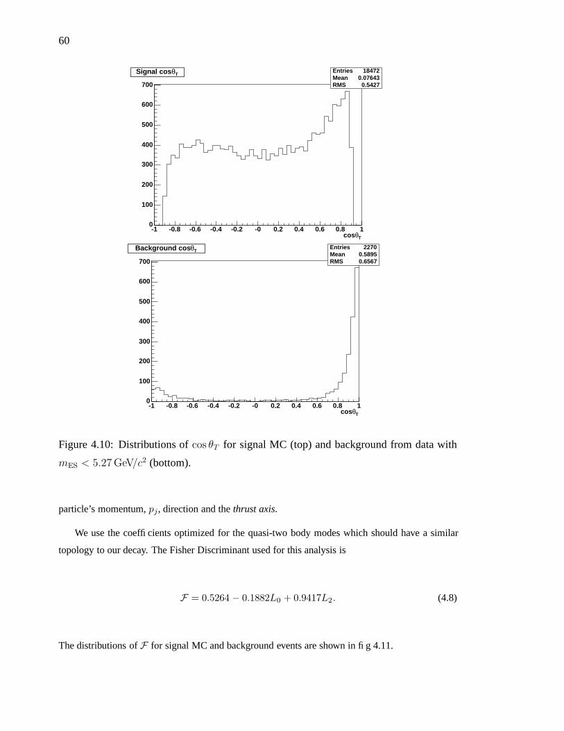
60

Tθ cos-1 -0.8 -0.6 -0.4 -0.2 -0 0.2 0.4 0.6 0.8 1

0

100

200

300

400

500

600

700

TθSignal cos Entries 18472Mean 0.07643RMS 0.5427

TθSignal cos

Tθ cos-1 -0.8 -0.6 -0.4 -0.2 -0 0.2 0.4 0.6 0.8 1

0

100

200

300

400

500

600

700

TθBackground cos Entries 2270Mean 0.5895RMS 0.6567

TθBackground cos

Figure 4.10: Distributions of cos θT for signal MC (top) and background from data with

mES < 5.27 GeV/c2 (bottom).

particle’s momentum, pj , direction and the thrust axis.

We use the coefficients optimized for the quasi-two body modes which should have a similar

topology to our decay. The Fisher Discriminant used for this analysis is

F = 0.5264 − 0.1882L0 + 0.9417L2. (4.8)

The distributions of F for signal MC and background events are shown in fig 4.11.

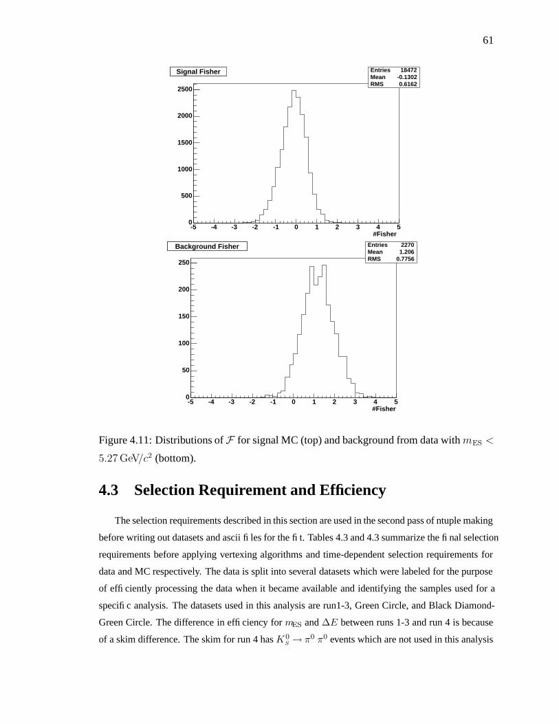
61

#Fisher -5 -4 -3 -2 -1 0 1 2 3 4 5

0

500

1000

1500

2000

2500

Signal Fisher Entries 18472Mean -0.1302RMS 0.6162

Signal Fisher

#Fisher-5 -4 -3 -2 -1 0 1 2 3 4 5

0

50

100

150

200

250

Background Fisher Entries 2270Mean 1.206RMS 0.7756

Background Fisher

Figure 4.11: Distributions of F for signal MC (top) and background from data with mES <

5.27 GeV/c2 (bottom).

4.3 Selection Requirement and Efficiency

The selection requirements described in this section are used in the second pass of ntuple making

before writing out datasets and ascii files for the fit. Tables 4.3 and 4.3 summarize the final selection

requirements before applying vertexing algorithms and time-dependent selection requirements for

data and MC respectively. The data is split into several datasets which were labeled for the purpose

of efficiently processing the data when it became available and identifying the samples used for a

specific analysis. The datasets used in this analysis are run1-3, Green Circle, and Black Diamond-

Green Circle. The difference in efficiency for mES and ∆E between runs 1-3 and run 4 is because

of a skim difference. The skim for run 4 has K0S → π0 π0 events which are not used in this analysis

62

and are essentially removed after the mES and ∆E selection requirements. The expected number

of signal and background events is 89 ± 10 and 439 ± 21 respectively which is the yield obtained

from a maximum likelihood fit to mES, ∆E, and F .

The level of B background is predicted to be negligible since scaling the B B MC sample, 14

events, from 520 fb−1 to 205 fb−1, we would expect 6 events. Of the 14 events in the full B B MC

sample, 4 are charmonium final states χc0 (3) and χc2 (1), which are removed explicitly. There are

then only 4 expected B background events in the data sample.

We choose to remove the χc events from our sample since they are known ccs events rather than

sqq events under study here. We remove events that fall within 3σ of the fitted mean mass of the

two χc modes. The fit to the two distributions is shown in fig 4.12. The mass cuts used are 3.3715 <

Mχc0 < 3.4708GeV/c and 3.5224 <Mχc2 < 3.6016GeV/c2. The branching fraction in the MC for

the two modes are 2x10−7 and 6x10−7 respectively. These decays have not been observed and only

a limit of B0 → χc0K0 < 5.0 × 10−4 at 90% confidence level has been measured experimentally.

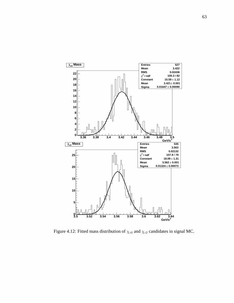
63

2GeV/c3.36 3.38 3.4 3.42 3.44 3.46 3.48 3.5

0

2

4

6

8

10

12

14

16

18

20

22

Massc0χ Entries 527Mean 3.422RMS 0.02436

/ ndf 2χ 100.3 / 82Constant 1.12± 15.59 Mean 0.001± 3.421 Sigma 0.00090± 0.01647

Massc0χ

2GeV/c3.5 3.52 3.54 3.56 3.58 3.6 3.62 3.640

5

10

15

20

25

Massc2χ Entries 535Mean 3.563RMS 0.02132


Massc2χ

Figure 4.12: Fitted mass distribution of χc0 and χc2 candidates in signal MC.

64

Table 4.3: Selection efficiency for analysis cuts in data. First Column for each category is the relative ε and the second column is

cumulative efficiency, ε.

Cut Run1-3 Data Run4 Data GC Run4 Data BD-GC Offres Run1-3 Offres Run1-4 BD

Total Events Before cuts 399,778 281,032 204,651 40,631 21,345

5.22 < mES < 5.3 GeV 74.2 74.2 66.7 66.7 66.4 66.4 53.5 53.5 47.2 47.2

|dE| < 120 MeV 36.2 26.9 28.7 19.2 28.5 18.9 34.4 18.4 27.6 13.0

K0S

flight length 0.2 < RD < 40 cm 14.5 3.9 15.2 2.9 16.0 3.0 14.3 2.6 14.4 1.9

K0S

mass 12 MeV 30.6 1.2 29.8 0.9 29.4 0.9 31.2 0.8 29.2 0.5

K0S

angle cut α < 200 mrad 32.5 0.4 31.4 0.3 30.0 0.3 27.2 0.2 29.9 0.2

| cos θT | < 0.9 40.7 0.2 38.2 0.1 41.1 0.1 37.4 0.1 25.7 0.04

K0S

vertex prob P (χ2) > 10−6 63.3 0.1 52.9 0.06 60.9 0.07 58.8 0.05 55.6 0.02

Luminosity 110.8 fb−1 55.0 fb−1 39.6 fb−1 11.6 fb−1 4.4 fb−1

Total # of Events After all cuts 401 155 137 20 5

# of Events/ fb−1 After all cuts 3.6±0.2 2.8±0.2 3.5±0.3 1.7±0.4 1.1±0.5

65

Table 4.4: Selection efficiency for analysis cuts in MC. First Column for each category is

the relative ε and the second column is cumulative efficiency, ε.

Cut Signal MC SP5 Signal MC SP6 bb MC

Total Events Before cuts 22,613 6,540 30,680

5.22 < mES < 5.3 GeV 81.1 81.1 81.5 81.5 68.3 68.3

|dE| < 120 MeV 84.8 68.8 84.5 68.9 22.7 15.5

K0S

flight length 0.2 < RD < 40 cm 88.0 60.5 87.9 60.6 10.4 1.6

K0S

mass 12 MeV 86.3 52.3 86.2 52.2 28.9 0.5

K0S

angle cut α < 200 mrad 94.2 49.2 93.5 48.8 54.9 0.3

| cos θT | < 0.9 87.6 43.1 88.2 43.0 79.5 0.2

K0S

vertex prob P (χ2) > 10−6 92.8 40.0 92.4 39.2 56.5 0.04

Luminosity/#Generated Signal MC 120 K 35 K 520 fb−1

Total # of Events After all cuts 9053 2563 14

66

4.4 Maximum Likelihood Fit

The time-dependent CP asymmetries for this analysis are extracted from a multidimensional

maximum likelihood fit. In this section we will describe the theory behind a maximum likelihood

fit and show the probability density functions (PDFs) used for each variable in the fit.

The likelihood for extracting N measurements x1, x2, ....xN given the PDF P for an observable

x is defined as

L(αj) =

N∏

i

P (xi|αj) (4.9)

where αj parametrize P . Maximizing L with respect to αj provides an unbiased, unique value. We

will use this fact to apply this method of extraction to our analysis.

The likelihood that describes the events in our sample is a multidimensional version of the

equation listed above. We will simultaneously fit several variable distributions, xk=mES, ∆E, F ,

∆t. If these variables are uncorrelated the probability of obtaining an event with a specific set of

measurements is the product of the individual probabilities

P (xk) = P (mES)P (∆E)P (F)P (∆t). (4.10)

Since we have signal and background events in our sample we can expand the total probability

to

P (xk) = fSPS(xk) + fBP

B(xk), (4.11)

where fS,B is the fraction of signal, background in the sample, fS = NS/(NS + NB) and fB =

NB/(NS +NB). Then the likelihood becomes:

L(αj, fS,B) =

NT∏

i

P ({xk}i|αj , fS,B). (4.12)

As it stands the likelihood does not take into account Poisson statistics. This can be remedied by

adding a Poisson termN ′

TNT e−N′

T

NT ! where N ′T = NS +NB . The extended likelihood becomes:

L(αj , fS,B) =e−N

′T

NT !

NT∏

i

NSPS({xk}i|αj) +NBP

B({xk}i|αj). (4.13)

From the likelihood fit we can extract the number of signal and background events and the fit

parameters αj which are the parameterizations of the background PDFs. In general the signal PDF

parametrization is fixed to values from the MC and allowed to float as a systematic uncertainty.

A loose estimate of the goodness of fit is estimated from χ2 = −2 logL + C(N ′T ) where

C(N ′T ) is a constant which dependents on the number of events extracted from the fit. We minimize

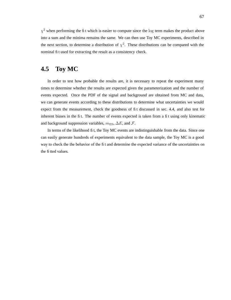
67

χ2 when performing the fit which is easier to compute since the log term makes the product above

into a sum and the minima remains the same. We can then use Toy MC experiments, described in

the next section, to determine a distribution of χ2. These distributions can be compared with the

nominal fit used for extracting the result as a consistency check.

4.5 Toy MC

In order to test how probable the results are, it is necessary to repeat the experiment many

times to determine whether the results are expected given the parameterization and the number of

events expected. Once the PDF of the signal and background are obtained from MC and data,

we can generate events according to these distributions to determine what uncertainties we would

expect from the measurement, check the goodness of fit discussed in sec. 4.4, and also test for

inherent biases in the fit. The number of events expected is taken from a fit using only kinematic

and background suppression variables, mES, ∆E, and F .

In terms of the likelihood fit, the Toy MC events are indistinguishable from the data. Since one

can easily generate hundreds of experiments equivalent to the data sample, the Toy MC is a good

way to check the the behavior of the fit and determine the expected variance of the uncertainties on

the fitted values.

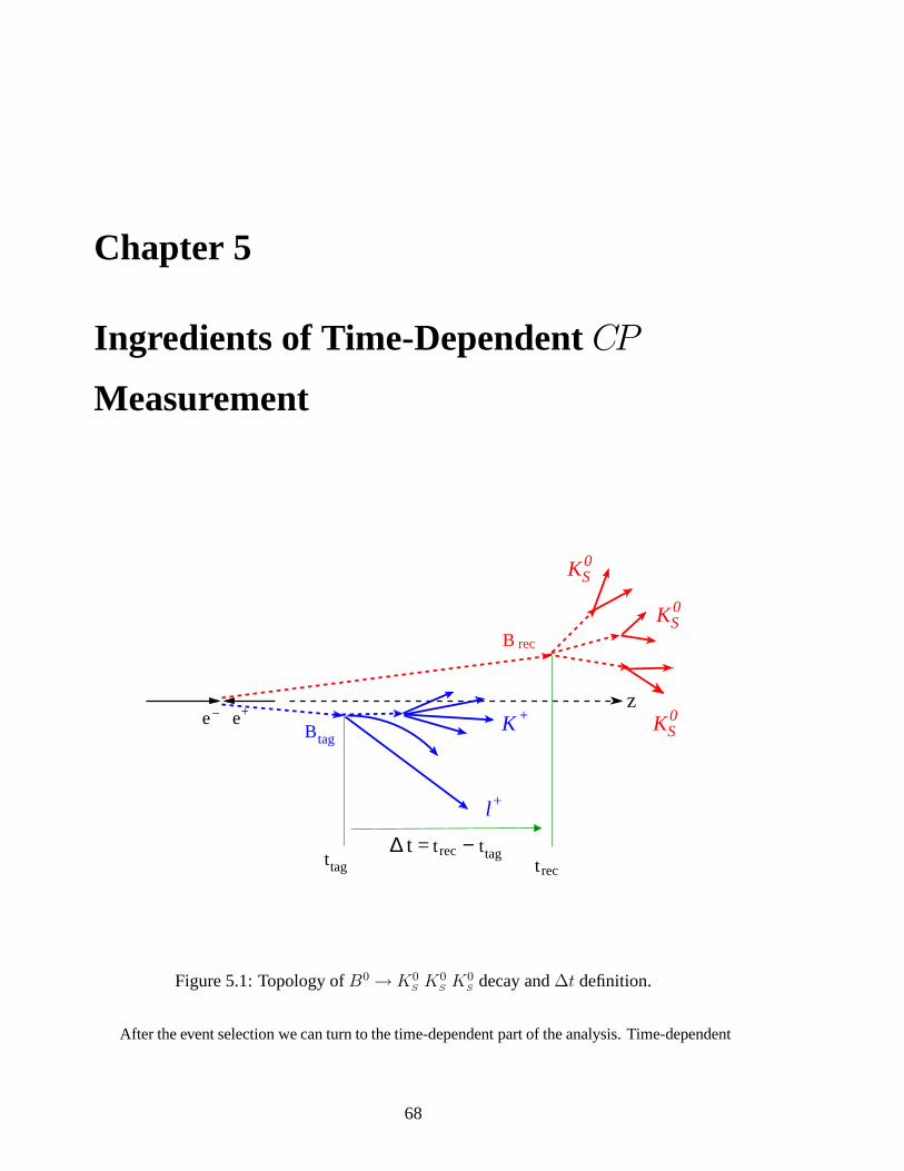
Chapter 5

Ingredients of Time-Dependent CP

Measurement

B

Btag

rec

ttag

KS0

t rec


KS0

KS0

e− +ez

l

K

+

+


SK0


After the event selection we can turn to the time-dependent part of the analysis. Time-dependent

68

69

CP measurements require three basic ingredients to measure the asymmetries. These ingredient

include determining the flavor of the other B meson in the Υ (4S) event, referred to as B tag, deter-

mining the decay vertex of each B meson, and finally converting the spatial separation of the two

B mesons into a proper time difference.

First we determine whether Btag decayed as a B0 or B0. This algorithm, which inclusively

reconstructs the tag side B, is called B tagging. A large sample of MC and data called the Bflav

sample is used to determine efficiencies and uncertainties in flavor identification. Once we know

the flavor of B tag as we saw in section 2.4.1, the flavor of the fully reconstructed B is determined

by the time difference of the decay of the two B mesons. This works because the B B system is in

an entangled state.

In addition to knowing the flavor of the tag side B we also need to have a decay vertex for both

B mesons to determine the proper time lapse between the decays. In decays like B 0 → J/ψK0S the

J/ψ is produced promptly so its decay vertex, reconstructed from precision tracking measurements

in the SVT, also determines the B decay vertex. Decays of K 0S mesons are generally not used

for determining the vertex since they they fly a significant distance from the primary B decay and

therefore cannot always be reconstructed with high enough precision.

A novel method, initially used for the decay of B0 → K0S π

0 [26], allows a vertex to be deter-

mined for the B decay by constraining the K0S vertex to the beamspot in the transverse direction,

which has a small uncertainty. This method is also applied to the B0 → K0S K

0S K

0S decay since

there are no primary charged tracks from which to determine a B vertex.

On the tag side, theB is reconstructed inclusively using charged tracks not used for reconstruct-

ing Brec. To determine the decay vertex of the B meson a geometric fit is done constraining the

particles to the beamspot. This is similar to what is done on the reconstructed side.

The boosted system, βγ = 0.55, makes the separation of the B vertices in z large enough that it

can be measured by the detector. Once ∆z is determined from the decay vertices of the B mesons,

it can be translated into a time difference ∆t by using the boost value and a simple conversion.

With the knowledge of ∆t and flavor of B tag the time spectrum can be fit. Because of detector

effects and uncertainties from the tagging algorithm, the theoretical ∆t spectrum has to be con-

volved with a resolution function which accounts for these effects. This is a method which is used

by all time-dependent CP measurements like J/ψ K 0S . However since the method of determining

the Brec vertex for this decay is different the resolution function must be checked to be the same as

that of nominally vertexed decays.

70

5.1 B Flavor Determination

It’s important to determine the B flavor of an event to great precision since the effective tagging

quality directly effects the error on the asymmetry S. There have been several generations of tagging

code at BABAR. Each generation aims to improve the efficiency of tagging and therefore involves

changing the algorithm. The tagging algorithm used in this analysis is called Tag04. This tagger

has an improved tagging capability of 0.5% over the previous version [27].

We mentioned earlier that the B tagging technique uses an inclusive method of reconstruction.

Fully reconstructing the event would be too inefficient given the small branching fractions and the

low efficiency for reconstructing all decay products. using an inclusive method gains efficiency but

at the expense of having a non-zero probability for assigning the wrong flavor.

The current algorithm used at BABAR is a neural network trained with a large sample of MC

events, from which the accuracy of the algorithm can be tested. In MC one knows the true flavor

and therefore can compare it with what the algorithm determines. There are several categories used

for determining the flavor. Each has its own efficiency and uncertainty. BABAR’s excellent particle

identification capability and ability to track particles of a wide range of momentum is essential to

determining the flavor of B tag.

We will describe the algorithm and the relevant terms needed to do B tagging in the next three

sections.

5.1.1 Definitions and Subtaggers

Several variables are used to characterize tagging and tagging performance. These are defined

as follows.

• Tagging Efficiency ε: Fraction of events for which a Btag is calculated.

• Tagging Efficiency Asymmetry ∆ε: Difference of tagging efficiency for B0 and B0: ∆ε ≡εB0 − εB0 .

• Mis-Tag Fractions w: Fraction of events tagged incorrectly by the tagging algorithm.

• Mis-Tag Fractions Asymmetry ∆w: Difference of mis-tag fraction for B0 and B0: ∆w ≡wB0 −wB0 .

• Dilution D : Attenuation of the CP asymmetry amplitude due to mis-tag, or tagging imper-

fection: D ≡ (1 − 2w).

71

• Effective Tagging Efficiency Q: Quality factor which summarizes the performance of tag-

ging: Q ≡ ε(1 − 2w)2.

• Effective Tagging Efficiency Asymmetry ∆Q: Difference of effective tagging efficiency

for B0 and B0: ∆Q ≡ QB0 −QB0 .

The error on S is effected by the value of the effective tagging efficiency, Q as seen from the

relation

σ(S) =1

√

QNsig

. (5.1)

Tag04 contains nine subtaggers which are shown in table 5.1.1. Each of the subtaggers utilizes

the correlation of the flavor of the B meson with its decay products, such as the charge of leptons,

kaons, soft pions, lambdas, and angle correlations between fast and slow tracks in the final state.

There are several discriminating variables used to determine the tag. This variables are applied after

all the tracks corresponding to Brec are removed. These variables are:

• p∗: Center of mass momentum of particle in question.

• EW90: Energy in the center-of-mass of B0 in a 90 degree cone defined around the direction of

the reconstructed virtual W boson.

• cos θmiss: In the B0 center-of-mass of Υ (4S) the angle between the lepton momentum and

the missing momentum of the tagging B.

• q: The charge of the track.

• Kid: Kaon particle identification.

• nK0S: Number of K0

S in event.

• LK: Kaon likelihood.

• cos θi,j: cosine of angle between particle i and j.

• cos θiThrust: cosine of the angle between particle i and the thrust axis in the center-of-mass

of Υ (4S).

There are other variables used for the Λ decay which include:

• MΛ: Reconstructed mass of the Λ.

• χ2Vertex: χ2 probability of the fitted Λ decay vertex.

72

• cosα: The cosine of the angle between the flight direction and the momentum vector of the

Λ .

• RD : Flight length of the Λ candidate before decay.

• pΛ,p : Momentum of track identified as a Λ or a p.

The discriminating variables for each subtagger are also listed in table 5.1.1.

Table 5.1: The nine subtaggers used in Tag04 tagger with the discriminating variables and

training goals.

Sub-tagger Category Discriminating Variables Training Recognition

Electron p∗, EW90 , cos θmiss, q B0 versus B0

Muon p∗, EW90 , cos θmiss, q B0 versus B0

KinLep p∗, EW90 , cos θmiss, q leptons from direct decays

Kaon K1id, K2

id, K3id, nK0

S,∑

pT B0 versus B0

Slow Pion p∗, cos θπThrust true slow pions

Max Pstar p∗, docaxy, cos θBCandmaxp∗fast tracks

KPI Kaon Tag, Slow Pion Tag, cos θK,π pairs of true K and slow π

FSC p∗slow/fasttrack, LKslow/fast, cos θslow/fast, fast-slow correlated tracks

cos θslow/fastThrust

Lambda MΛ, χ2Vertex, cosα, RD, pΛ, pproton Lambda decays

The variables contain discriminating physics information to classify the flavor of B tag. There

are underlying physics signatures which determine the flavor. In general we can separate them into

four categories of which the nine subtaggers try to recognize variations to obtain greater Q. The

four categories are leptons, kaons, soft and hard pions from D∗ decays, and Λ decays. We will

describe then in the next four sections.

Leptons

Fig. 5.2 shows the Feynman diagram for semileptonic decays producing primary or secondary

leptons from the cascade process b → c → s. The sign of the primary leptons can distinguish the

flavor of the B decay. A positive sign primary lepton indicates a B 0 decay while a negative sign

73

b c u,

νl

l+

W+

d d

b

W+

νl

s

W��

��

a) b)

d d

c

l−

−

Figure 5.2: Feynman diagram for a B decay producing a primary lepton a), or secondary

lepton with opposite charge from the cascade process b→ c→ s b).

lepton is derived from a B0 decay. This correlation gives a very clean tagging signal with very low

mistag rates. The fact that about 10% of all B mesons decay semileptonically makes for a large tag-

ging sample. Sources of mistag can arise from secondary lepton decays and hadrons misidentified

as leptons, fake leptons. A requirement that p∗ for the lepton exceed 1.4GeV/c removes almost all

secondary and fake leptons.

Kaons from cascade b→ c→ s decays

cs

u

+Kb

0

W+

W−

+K K −

u

dπ −d

B

c,u

s u

s

Figure 5.3: Sources of charged kaons in the decay of a B0 meson.

Fig. 5.3 shows the Feynman diagram of B0 decays to kaons and pions. In the cascade decay

of b → c → s a maximum of three kaons can be produced. Depending on the source of the kaon,

it can either be right-sign or wrong-sign. The right-sign kaons come from hadronization of the s

quark in the b→ c→ s reaction producing a K+. A right-sign kaon can also be produced from the

W+ hadronization to a K+. A wrong-sign Kaon, K− can be produced from the W− hadronization

in the secondary decay of the intermediate charm meson state.

The W boson hadronization into kaons is Cabibbo-suppressed (|Vus|2 ∼ 0.04) and decays

into pions or D+s /− ≡ cs are favored. The D+

s /− can be reconstructed inclusively for tagging

information. The main source of mistag using kaons is from the presence of the wrong sign kaon

74

and misidentifying pions as kaons.

Soft and hard pions from D∗ decays

W+

c

u

b

d

0B

,ρ +1,a+π+

h

d

u

dd

u

D

Dc

*_

0

_πs

Figure 5.4: The B0 → D∗−π+, ρ+, a+1 decay. The charge of the soft pion πs and that of the

direct pion πh are correlated with the flavor of the neutral B meson.

Fig. 5.4 shows decays of B0 → D∗ π+, ρ+, and a1+. The sign of the pion hadronizing from

the W boson, πh, has the right sign correlation with Btag meson. This pion is called a hard pion

since it has a large momentum.

The pion from the D∗ decay, πs, has the wrong sign correlation with Btag and it can be distin-

guished from πh by its momentum. The πs is called the soft pion, because of its low momentum.

This pion has a low momentum because theD∗ andDmasses differ by only 146 MeV, and therefore

the energy available in the decay is small making the pion soft. The soft pion can be reconstructed

inclusively using angular correlations between low momentum tracks and D0 mesons.

Λ Decays

The quark content of the Λ baryon is uds. Cascade decays of b→ c→ s can produce Λmesons

which need to be distinguished from kaon decays. Even though the Q of this subtagger is small,

removing this subtagger would reduce the overall Q by 0.38 which is a non-negligible effect. Tag04

is the first tagger which uses this subtagger to distinguish the flavor of Brec.

5.1.2 Algorithm

Tag04 is a multivariate tagging algorithm exploiting the physics characteristics of the Btag de-

cay. It contains nine sub-taggers and assigns the events to six hierarchical, mutually exclusive

75

Electron

Kin. Lepton

Muon

Kaon

Slow Pion

Lambda

Max p*

KPi

FSC

Slow Pion

Single Kaon

BT

agger

Tag04

Lepton

Kaon I

Kaon II

Kaon & Pion

Pion

Others

r2r1_i

Figure 5.5: The schematic drawing of the subtaggers and tagging categories of Tag04. The

outputs ri1 and r2 are described in the text.

categories which group events characterized by similar mis-tag fractions and underlying physics.

The structure of Tag04 is shown in 5.5 and the definition of the tagging categories for Tag04 are

shown in table 5.2.

Each subtagger provides a continuous output variable r i1 which runs between +1 and -1. Elec-

tronTag and MuonTag in the table corresponds to r1 values from the Electron and Muon subtaggers

respectively. Candidates with r1 close to +1(-1) are more likely to beB0 (B0). The r2 output values,

or Tag04 output, are also continuous between +1 and -1. The btgtag in table 5.2 corresponds to r2

output. In the r2 layer the outputs of the subtaggers are combined into the tagging categories.

A large sample of MC is used to train the subtaggers. The training procedure has access to the

true flavor of B tag and therefore can estimate piw, the mistag probability for each subtagger. Each

subtagger will have a different piw which is governed by the physics of that selection.

There are six mutually exclusive tagging categories Lepton, Kaon I, Kaon II, Kaon & Pion,

and Others with names that are meant to reflect the underlying dominant physics process for each

category. Tag04 has the feature that each subtagger neural network is optimized for the specific

subtagger instead of the total output from all tagging categories. The output of Tag04 is shown in

fig 5.6.

5.1.3 Algorithm Performance

The performance of the Tag04 B flavor tagging algorithm in MC events is shown in table 5.3.

These results are measured from a large sample of MC events with one B meson decaying to flavor

76

Table 5.2: Category definition used by BTagger Tag04.

Category Cuts on input tags

Lepton |btgtag| > 0.8 and (|ElectronTag| > 0.7 .or. |MuonTag| > 0.7)

Kaon I |btgtag| > 0.8 and (|ElectronTag| < 0.7 .and. |MuonTag| < 0.7)

Kaon II |btgtag| > 0.6

Kaon&Pion |btgtag| > 0.4

Pion |btgtag| > 0.2

Others |btgtag| > 0.1

BtgTag outputBtgTag output

0

1000

2000

3000

4000

5000

6000

7000

-1 -0.8 -0.6 -0.4 -0.2 0 0.2 0.4 0.6 0.8 1

Figure 5.6: The Tag04 Neural Network output. The red and blue histograms denote true

B0 and B0 tags respectively.

eigenstates.

The ∆ tagging parameters takes into account asymmetries in tagging B0 versus B0 events.

From the table above we can make some observations about the tagging categories and general

tagging performance at BABAR.

• About 3/4 of all selected B candidates are assigned a flavor tag.

• As expected, the Lepton category has the smallest mistag rate.

• The Kaon II category has the largest efficiency.

• The best Q comes from the Lepton, Kaon I, and Kaon II categories.

77

• The largest mistag asymmetry comes from the Pions category. This is due to different recon-

struction efficiencies of positive and negative soft pions.

The values listed above are parameters used in the maximum likelihood fit for fitting MC events.

The tagging parameters are slightly different for data and we therefore have to use those parameters

when fitting data events. There is a large sample of data events, flavor sample, with fully recon-

structed flavor eigenstates which is used for determining the tagging parameters. The parameters

can differ between data and MC because of differences in reconstruction and particle identification

efficiencies. In general the efficiencies in MC are better than in data and therefore using values from

MC to fit data would give unrealistic results. Additionally the branching fractions for many decays

used in MC have not been measured experimentally and are generated using theoretical values. This

can result in different rates of kaons and leptons between MC and data which translates into differ-

ent mistag rates. The tagging parameters used in the maximum likelihood fit are slightly different

than the ones shown here. The values used to fit data and MC samples can be found in table 6.1.2

in section 6.1.2.

5.1.4 Effect of Tagging Imperfections

In this section we show how tagging imperfections effect what we observe experimentally. We

will start with the definitions used in chapter 2 and modify the probability distributions in the pres-

ence of mistagging and efficiencies of each tagging category.

In section 2.4.1 we introduced the time-dependent probability distributions forB meson mixing.

We can now use these arguments to write the time-dependent probability distributions of B decays

to tagged flavor eigenstates:

ΓB0,B0(∆t) = ΓB0,B0(∆t) =e−|∆t|/τ

4τ(1 + cos(∆md∆t)), (5.2)

ΓB0,B0(∆t) = ΓB0,B0(∆t) =e−|∆t|/τ

4τ(1 − cos(∆md∆t)), (5.3)

where ΓA,B means an event with one B tagged as B and the other reconstructed as A. If A = B

the event is unmixed otherwise it is mixed. Using these definitions then the probability of observing

an event with a tagged flavor T = ±(+ = B 0and− = B0) for one B and a reconstructed flavor

R = ± for the other B in tagging category i is

Pi(∆t, T,R) =2εri(R)

〈εri 〉[εti(T )(1 − wi(T ))ΓR,T + εti(−T )(wi(−T ))ΓR,−T ], (5.4)

78

where 〈εri 〉 ≡ εi+−εi−2 . The first term above takes into account the correct tagged events and the

second term is for the wrong tagged events. Then when normalizing such that∑

T,R Pi(∆t, T,R) =

εti we get the expression

Pi(∆t, T,R) =e−|∆t|/τ 〈εti〉

4τ

1 +Rνi1 − µiνiξ

×

[(µiTDi + 1 + T∆Di) −

(TDi + µi(1 + T∆tDi))R cos(∆md∆t)] (5.5)

where ξ ≡ 11+(τ∆tmd)2

, µ ≡ ∆εr

(εr++εr−) , and 〈εt〉 ≡ (εt+ + εt−)/2.

Assuming the reconstructed B mesons are CP eigenstates we obtain the following expression

with tagging imperfections taken into account,

P (∆t, T ; qi) =εti4τ

1

1 − µiξCfe−

|∆t|τ ×

([µiTDi + (1 + T∆Di

2)] + [TDi + µi(1 + T

∆Di

2)]A(∆t)), (5.6)

where A(t) ≡ Sf sin (∆md∆t) ∓ Cf cos (∆md∆t). To determine the effect of the imperfections

of the tagging algorithm we set νi = µi = ∆Di = 0 in this equation to get

Pi(∆t, T ) =εti4τe−

|∆t|τ [1 + TDi (Sf sin (∆md∆t) ∓Cf cos (∆md∆t))] . (5.7)

We see that the tagging mistakes only effect the amplitude of the sine and cosine term by the dilution

Di.

5.2 Measuring Decay Time, ∆t

To determine the decay time difference ∆t between the two B mesons in the event we need to

find the decay vertex of both B mesons, Btag and Brec. Once the z position is determined for each

decay vertex we can compute ∆z which is defined as ∆zrec − ∆ztag . Because we know the boost

of the Υ (4S) system we can then compute ∆t from ∆z by a simple conversion.

Remember that we can measure ∆z because the Υ (4S) system is boosted in the high energy

beam direction. In the Υ (4S) rest frame βγ ∼ 0.06 and with the B lifetime of 1.5 ps the B mesons

would be separated by only about 34µm. This separation is too small to be measured experimentally

however. So by boosting the system to βγ = 0.55 we get a separation of about 260µm in the z

direction. The vertex resolution of the SVT is good enough to measure such separation quite easily.

79

The B pair from Υ (4S) is in a entangled or correlated state. This means that until one B decays

there will always be one B0 and one B0. If at time t = ttag Btag = B0 then Brec = B0 if Btag

decayed before Brec. Since ∆t ≡ trec − ttag, ∆t > 0 if Brec decayed after Btag and ∆t < 0 if

Brec decayed before Btag. The boundary condition is set at ttag however since at this time we know

whether Btag was a B0 or B0. If Brec = B0 at t = ttag then the time evolution of Brec is given by

|B0rec(∆t)〉 = (p/q)g−(∆t)|B0〉 + g+(∆t)|B0〉 (5.8)

g−(t) = e−iMte−iΓt/2i sin(∆mt/2) (5.9)

g+(t) = e−iMte−iΓt/2 cos(∆mt/2). (5.10)

We call an event mixed if at t = trec Brec=B0. Otherwise, ifBrec=B0 the flavor stayed the same and

is therefore called unmixed. We therefore see that we do not need to know any information about

the decay time of the Υ (4S) which has a great experimental advantage.

5.2.1 Btag Vertex

Figure 5.7: Schematic view of the Υ (4S) → BB decay in the y-z plane. Note that the

scale in the y direction is substantially magnified compared to that in the z direction for

illustration purposes.

The decay vertex of Btag is reconstructed using an inclusive method which uses charged tracks

in the event other than those required for the reconstruction of Brec. The algorithm removes charged

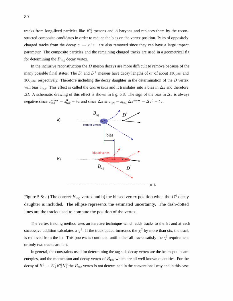
80

tracks from long-lived particles like K0S mesons and Λ baryons and replaces them by the recon-

structed composite candidates in order to reduce the bias on the vertex position. Pairs of oppositely

charged tracks from the decay γ → e+e− are also removed since they can have a large impact

parameter. The composite particles and the remaining charged tracks are used in a geometrical fit

for determining the Btag decay vertex.

In the inclusive reconstruction the D meson decays are more difficult to remove because of the

many possible final states. The D0 and D+ mesons have decay lengths of cτ of about 130µm and

300µm respectively. Therefore including the decay daughter in the determination of the B vertex

will bias ztag. This effect is called the charm bias and it translates into a bias in ∆z and therefore

∆t. A schematic drawing of this effect is shown in fig. 5.8. The sign of the bias in ∆z is always

negative since zmeastag = z0tag + δz and since ∆z ≡ zrec − ztag ∆zmeas = ∆z0 − δz.

tagB

tagB

D0

z

D0

a)

b)

bias

correct vertex

biased vertex

Figure 5.8: a) The correct Btag vertex and b) the biased vertex position when the D0 decay

daughter is included. The ellipse represents the estimated uncertainty. The dash-dotted

lines are the tracks used to compute the position of the vertex.

The vertex finding method uses an iterative technique which adds tracks to the fit and at each

successive addition calculates a χ2. If the track added increases the χ2 by more than six, the track

is removed from the fit. This process is continued until either all tracks satisfy the χ2 requirement

or only two tracks are left.

In general, the constraints used for determining the tag side decay vertex are the beamspot, beam

energies, and the momentum and decay vertex of Brec which are all well known quantities. For the

decay ofB0 → K0SK

0SK

0S the Brec vertex is not determined in the conventional way and in this case

81

will not provide as good a constraint on Btag. We will discuss this in more detail in section 5.2.2.

The intersection of the momentum vector of Btag with the beamspot gives the position of the Υ (4S)

decay to B pairs. The momentum of the Υ (4S) is determined from the beam energies; momentum

conservation then gives ~ptag = ~pΥ (4S) − ~prec. The Υ (4S) decay vertex and the momentum of Btag

are then used in a fit as kinematic and geometric constraints to determine the Btag vertex. This

method produces a ztag resolution of about 180µm.

5.2.2 Brec Vertex

Since the decay of B0 → K0S K

0S K

0S has only charged tracks from long lived K0

S mesons, the

vertex cannot be determined in the conventional way. The best constraint we have is the beamspot

which is known to great precision in the transverse plane, 4µm vertically and 150µm horizontally.

Therefore we can do a geometric fit constraining the B meson production vertex to the beamspot,

called TreeFitter vertexing. This method gives an average uncertainty on ztag of 75µm as deter-

mined from signal MC events.

This method of constraining the reconstructed B meson to the beamspot was pioneered for the

B0 →K0S π

0 measurement [26]. The first published results were done using a vertexing technique

which constrained the B decay vertex instead of the production vertex of the B to the beamspot,

called beam constrained vertexing, (BC) vertexing. Fig 5.9 shows a schematic drawing of the two

vertexing methods. The beamspot is shown as a green ellipse and the transverse size has been

exaggerated for display purposes.

By constraining the decay vertex to the beamspot, one ignores the transverse motion of the

B meson and therefore cannot accurately estimate the uncertainty on the vertex position in the

transverse direction. This effect is especially noticeable in the vertical direction where the resolution

is small enough to see the B motion which is about 30µm. This can be seen in fig 5.10 where the

pull distributions for the vertex are shown for the two vertexing methods. The pull for a variable x

is defined as xpull ≡ xi−xσxi

, where x is the average of the distribution of xi. Notice the non-Gaussian

shape of the y vertex pull for the BC vertexed events. All other pull distributions have an expected

width. In the main analysis we use the TreeFitter vertexing method but as a cross-check we will

also do a fit using values from the BC vertexing technique as well.

Although the error on zrec using the two techniques discussed in this section is larger than

for B decays with prompt tracks, the uncertainty on ∆z is still dominated by ztag determination.

Therefore we will see in section 5.3 that the resolution is comparable to that in B 0 → J/ψ K0S .

82

5.2.3 Extracting Decay Time Difference

Since the Υ (4S) system is boosted in the z direction by βγ = 0.55 the average separation of

the B meson vertices is about 260µm. The value of ∆z is determined directly by the Btag vertex fit

to correctly determine correlations in variables. The fit also provides the uncertainty on ∆z, σ∆z,

by taking into account the correlations between the B vertices.

A simple estimate of the time difference ∆t is given by

∆z = βγc∆t (5.11)

where βγ = 0.55 and is known with a precision of 0.1%. However this relation only holds if the

boost is only in the z direction and the B mesons are at rest in the Υ (4S) frame. However, the boost

axis is actually rotated by 20 mrad with respect to the detector z axis and the momentum of the B

meson is actually about 340 MeV/c in the Υ (4S) rest frame.

Correcting for these effects, the ∆z relation then becomes

∆z = βγγ∗recc∆t+ γβ∗recγ

∗rec cos θ∗recc〈trec + ttag〉 (5.12)

where θ∗rec, β∗rec, and γ∗rec are the polar angle, the velocity, and the boost factor of Brec in the Υ (4S)

frame respectively. The expected value of the sum of the decay times is 〈trec + ttag〉 which can be

estimated by

〈trec + ttag〉 = τB + |∆t|. (5.13)

The difference in ∆t computing with the two different relations has an an RMS spread of 0.20

ps which is small compared to the B0 lifetime of 1.542 ± 0.016. The resolution on ∆t improves

by about 5% when using 5.12.

The pull distributions for ∆t and ∆z are shown in fig 5.2.3 and they all have widths close to

one as expected.

5.3 ∆t Resolution Function

In fitting the ∆t decay distributions we must take into account the ∆t resolution from the mea-

surement of the B vertex locations. The ∆t PDF 2.50 is convolved with the resolution function to

model the impact of the detector effects on the ∆t function. The resolution function is parameter-

ized as a sum of three Gaussian distributions (listed in order of increasing width as core, tail, and

outlier) as a function of the ∆t residual δt ≡ ∆tmeas−∆ttrue and the uncertainty on ∆t, σ∆t. The

83

functional form of the resolution function is:

R(δt, σ∆t, vi) =∑

k=core,tail

fk

skσ∆t

√2πe

(

(δt−bik

σ∆t)2

2(skσ∆t)

)

+fout

σout√

2πe

(

δ2t2σ2

out

)

(5.14)

where the parameters vi are:

• bcore,tail : The core, tail bias scale factor.

• score,tail : The core, tail sigma scale factor.

• ftail,out : The fraction of events in the tail, outlier Gaussian.

• σout : The width of the outlier Gaussian fixed to 8 ps.

The parameters of the ∆t resolution function are determined from signal B 0 → K0S K

0S K

0S MC

and for the background they are determined from the maximum likelihood fit.

The functional form of the resolution function allows for a global scaling of the event-by-event

estimated errors σ∆t in both the core and tail Gaussian distributions, as well as a charm bias offset

that is also expected to be proportional to σ∆t. The effective widths, σ, and biases, δ0, of the core

and tail components can be written as

σcore,tail = Score,tailσ∆t, (5.15)

δ0core,tail = bcore,tailσ∆t. (5.16)

Fig 5.12 shows the relation of σ∆t to the mean and RMS spread of δt for MC events with a regular

decay vertex like the B0 → J/ψ K0S decay. We will show that the B0 →K0

S K0S K

0S decay has the

same relations between the δt, σ∆t, and the true ∆t and therefore the same functional form of the

resolution function can be used.

As already noted, the tag side vertex is biased due to inclusion of displaced tracks from charm

decays. If the direction of the decay of the D meson is the same as the boost direction of the B, the

bias along the z direction is enhanced as shown in fig. 5.13. D mesons decaying perpendicular to

the flight direction of B have a better z resolution and the least bias in the B tag vertex. The effect

of the bias is seen clearly in fig 5.12b where for large values of σ∆t the residual is about −0.2 ps.

The outlier Gaussian has no bias and scaling of its width. It has a fixed width of 8 ps and

typically accounts for only a few percent of the events.

84

5.3.1 Comparison of B0 → K0SK0

SK0

SDecays with Other Decays

In order to use the same resolution function as described in section 5.3 we must confirm that

correlations of the residual and σ∆t are the same as regularly vertexed events. This will be discussed

in more detail in section 6.1.1.

We also need to show that the σ∆t distribution is about the same as regularly vertexed events.

The error on the ztag is usually about 180µm and is the dominant contribution to the error on ∆t for

regularly vertexed decays. If the TreeFitter vertexing is to give similar results the ∆t error should

still receive its major contribution from the tag side. In other words zrec needs to be reconstructed

with a better resolution than ztag . In order for this to happen we need at least one K 0S decaying

within the SVT. If none of the K0S mesons decay inside the SVT the event cannot be used for a time

dependent measurement.

In comparison to the decay B0 →K0S π

0 decay, which was the first to use this vertexing method,

the K0S mesons in B0 → K0

S K0S K0

S have lower average momentum and they therefore have a

higher probability of decaying in the SVT. We also only need one K 0S to reconstruct the vertex so

the multiplicity of K0S mesons in this decay helps in obtaining a higher fraction of events which

decay in the SVT.

In section 5.3.2 we will compare the σ∆t distributions forB0 → K0SK

0SK

0S and regular vertexed

events.

5.3.2 σ∆t and Classes

Events reconstructed with the TreeFitter vertexing method are classified based on their σ∆t

values which also correspond to the hit pattern within the SVT. Since the K 0S mesons have a long

lifetime they may decay within the DCH or the outer layers of the SVT. The SVT structure is such

that the extrapolation precision is achieved if there are hits in the first three layers closest to the

beampipe. The outer two layers are mainly used to extrapolate the tracks within the DCH and are

therefore placed further from the event vertex. Therefore the classes are defined as:

• Class I: Decays where both pions have at least one φ and one z hit in any of the first three

inner SVT layers.

• Class II: Decays where both pions have at least one φ and one z hit in the SVT but are not in

Class I. These events correspond to K0S decays beyond the inner three SVT layers.

• Class III: Decays where either of the two pions have at least one SVT hit, but do not satisfy

the requirements of Class I or II.

85

• Class IV: Decays where neither pion has SVT hits.

Fig 5.14 shows σ∆t versus the shortest flight distance in the x-y plane for the three K 0S mesons

in the event. We see that if the K0S decayed after the third SVT layer the error becomes larger as

expected. The fourth and fifth layer of the SVT have worse resolution than the first three layers of

the SVT. In this analysis and in all BABAR time-dependent analysis only events with σ∆t < 2.5 ps

and |∆t| < 20 ps are used.

Fig. 5.15 shows the ∆t error distribution for Bflav MC events and comparison of nominally

vertexed events in data and MC. Fig 5.16 shows the corresponding error distribution for SP5 and

SP6 B0 → K0S K

0S K

0S MC and data divided into different classes of events. We see that when at

least one K0S is in Class I the ∆t error distribution is similar to regularly vertexed events. Events

with no Class I but at least one Class II K0S can be used for the fit since their ∆t resolution is

similar to that of decays with prompt particles. In all 99.9% of events have at least one Class I

or Class II K0S . For the B0 → K0

S π0 decay only about 63% of events can be used for the time-

dependent fit. Given the smaller branching for B0 →K0S K

0S K

0S (6.9 × 10−6 versus 11.4 × 10−6)

the new channel provides a measurement with competitive precision because of the much higher

vertex reconstruction efficiency.

Events in Class III or Class IV cannot be used since the error for these class of events is too

large.

86

Table 5.3: Tag04 performance from MC events in the 6 tagging categories and the total. The tagging parameters are defined in

section 5.1.1

Category ε(%) ∆ε(%) ω(%) ∆ω(%) Q(%) ∆Q(%)

Leptons 9.1 ± 0.1 0.1 ± 0.2 2.8 ± 0.1 0.0 ± 0.3 8.2 ± 0.1 0.1 ± 0.2

Kaon I 11.4 ± 0.1 −0.2 ± 0.2 6.2 ± 0.2 0.3 ± 0.4 8.8 ± 0.1 −0.3 ± 0.2

Kaon II 17.4 ± 0.1 0.3 ± 0.2 15.7 ± 0.2 −0.2 ± 0.5 8.2 ± 0.1 0.2 ± 0.2

Kaons and Pions 13.9 ± 0.1 0.3 ± 0.2 25.6 ± 0.3 −1.8 ± 0.6 3.3 ± 0.1 0.6 ± 0.2

Pions 14.3 ± 0.1 −0.5 ± 0.2 34.8 ± 0.3 7.2 ± 0.7 1.4 ± 0.1 −1.3 ± 0.1

Others 9.4 ± 0.1 0.0 ± 0.2 41.8 ± 0.4 5.0 ± 0.8 0.3 ± 0.0 −0.3 ± 0.1

Total 75.5 ± 0.2 0.0 ± 0.5 30.1 ± 0.2 −1.0 ± 0.4

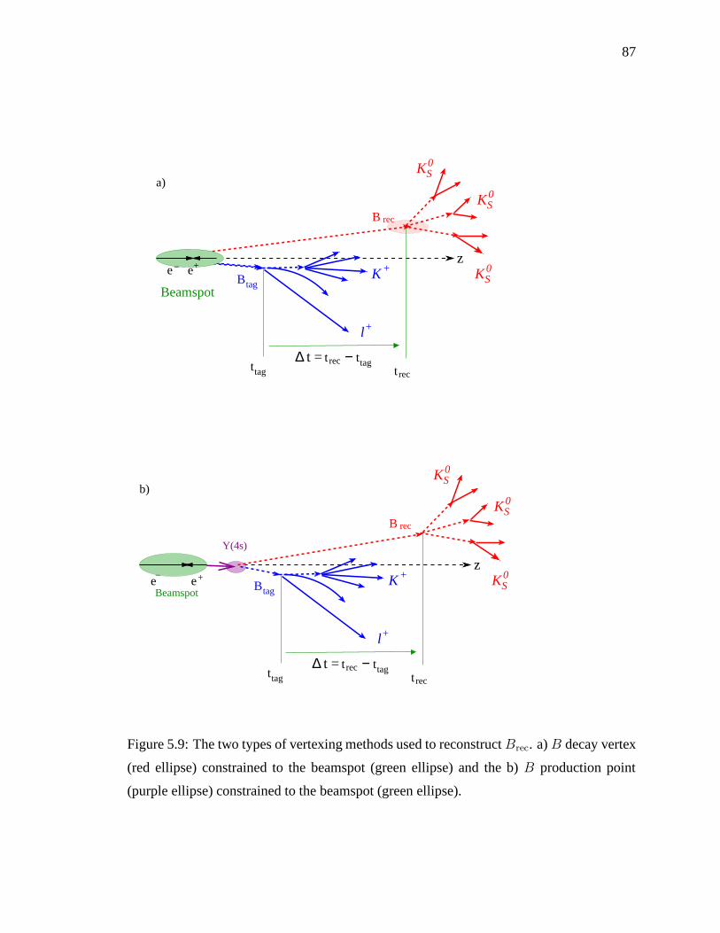
87

B

Btag

rec

Beamspot

ttag

KS0

t rec


KS0

KS0

e− +ez

l

K

+

+

a)

B

Btag

rec

Y(4s)

Beamspot

ttag

KS0

t rec


KS0

KS0

z

l

K

+

+e− e+

b)

Figure 5.9: The two types of vertexing methods used to reconstruct Brec. a) B decay vertex

(red ellipse) constrained to the beamspot (green ellipse) and the b) B production point

(purple ellipse) constrained to the beamspot (green ellipse).

88

-5 -4 -3 -2 -1 0 1 2 3 4 50

50

100

150

200

250

300

350

400

pull in x F hpullxEntries 9728Mean 0.03493RMS 1.123


pull in x F

-5 -4 -3 -2 -1 0 1 2 3 4 50

50

100

150

200

250

300

350

400

pull in x TF hpullxEntries 9736Mean 0.01122RMS 1.139

/ ndf 2χ 259.9 / 96Constant 4.9�± 363 Mean 0.01063�± 0.01478 Sigma 0.009�± 1.027

pull in x TF

-5 -4 -3 -2 -1 0 1 2 3 4 50

100

200

300

400

500

600

700

pull in y F hpullyEntries 9751Mean 0.009324RMS 0.9215

/ ndf 2χ 852.6 / 95Constant 8.6�± 511.1 Mean 0.00734�± 0.01232 Sigma 0.0089�± 0.6899

pull in y F

-5 -4 -3 -2 -1 0 1 2 3 4 50

50

100

150

200

250

300

350

400

pull in y TF hpullyEntries 9731Mean -0.002966RMS 1.11

/ ndf 2χ 279.7 / 97Constant 5.2�± 378.1 Mean 0.010183�± -0.009533

Sigma 0.0089�± 0.9826

pull in y TF

-5 -4 -3 -2 -1 0 1 2 3 4 50

50

100

150

200

250

300

350

400

pull in z F hpullzEntries 9707Mean 0.02759RMS 1.184


pull in z F

-5 -4 -3 -2 -1 0 1 2 3 4 50

50

100

150

200

250

300

350

400

pull in z TF hpullzEntries 9715Mean 0.0146RMS 1.195


pull in z TF

Figure 5.10: Pull distributions in x, y, and z of the decay vertex position of the B0 →K0

SK0

SK0

Sdecay using BC vertexing (F) (left) and TreeFitter (TF) (right).

89

-10 -8 -6 -4 -2 0 2 4 6 8 100

100

200

300

400

500

600

t Pull TF Good Ks Vertex∆ hpulltpiEntries 8410

Mean -0.2806

RMS 1.375

/ ndf 2χ 241.2 / 80

Constant 8.2�± 559.2

Mean 0.0131�± -0.2292

Sigma 0.011�± 1.166

t Pull TF Good Ks Vertex∆

-10 -8 -6 -4 -2 0 2 4 6 8 100

100

200

300

400

500

600

z Pull TF Good Ks Vertex∆ hpullzpiEntries 8410

Mean -0.2802

RMS 1.362

/ ndf 2χ 215.7 / 76


Mean 0.0129�± -0.2284

Sigma 0.011�± 1.153

z Pull TF Good Ks Vertex∆

-10 -8 -6 -4 -2 0 2 4 6 8 100

100

200

300

400

500

600

t Pull F Good Ks Vertex∆ hpulltpiEntries 8416

Mean -0.2941

RMS 1.359

/ ndf 2χ 231.3 / 77


Mean 0.0129�± -0.2472

Sigma 0.011�± 1.152

t Pull F Good Ks Vertex∆

-10 -8 -6 -4 -2 0 2 4 6 8 100

100

200

300

400

500

600

z Pull F Good Ks Vertex∆ hpullzpiEntries 8416

Mean -0.2939

RMS 1.347

/ ndf 2χ 218.3 / 80


Mean 0.0127�± -0.2482

Sigma 0.011�± 1.141

z Pull F Good Ks Vertex∆

Figure 5.11: The ∆z and ∆t pull distributions for TreeFitter (TF) and BC vertexing (F).

(ps)t∆σ0.4 0.6 0.8 1 1.2 1.4 1.6 1.8 2 2.2 2.4

t res

idua

l RM

S (p

s)

∆

0.5

1

1.5

2

2.5a)

(ps)t∆σ0.4 0.6 0.8 1 1.2 1.4 1.6 1.8 2 2.2 2.4

t res

idua

l (ps

)

∆M

ean

of

-0.35

-0.3

-0.25

-0.2

-0.15

-0.1 b)

Figure 5.12: Correlation between σ∆t and a) the RMS spread and b) the mean of the resid-

ual δt = ∆tmeas − ∆ttrue in simulated events with a decay vertex on the Brec side.

90

tagB

tagB

D0

D0

σtag

σtag

bias

z

a)

b)

Figure 5.13: Correlation between the bias of the Btag vertex and its uncertainty σtag when

a) the D0 flies in the boost direction of Btag, or b) the D0 is perpendicular to the boost

direction of Btag.

Ks dr cm0 2 4 6 8 10 12 14 16 18 20

t)

ps

∆(σ

0

1

2

3

4

5

Ks Decay LengthKs Decay Length

Figure 5.14: Projection plot of σ∆t versus the flight distance of the K0S

in the event with the

smallest flight length. Distribution of the K0S

flight length in x − y is shown by the filled

histogram. The red arrows mark the location of SVT layers.

91

0

500

1000

0 0.5 1 1.5 2

∆t error (ps)

Ent

ries

/0.0

6 ps B0 → D(*) - π+,ρ+,a

1 +a)

0

50

100

0 0.5 1 1.5 2

∆t error (ps)

Ent

ries

/0.0

6 ps B0 → J/ψKS

0

B0 → ψ(2S)KS0

B0 → χc1KS0

B0 → J/ψK*0

b)

Figure 5.15: Distribution of σ∆t for a) the Bflav sample excluding the J/ψK∗0(K+π−)

mode and b)BCP the sample together with the J/ψK∗0 mode. Points are from data and the

open histogram is the expected distribution from Monte Carlo simulation.

92

ps0.5 1 1.5 2 2.5 3

0

50

100

150

200

250

300

350

400

450

T) TF Good Ks Vertex SP5MC∆(σ Entries 8684Mean 0.903RMS 0.4643

At least 1 class 1

All class 1

At least 1 class 2

No Class 1; At least 1 class 2

T) TF Good Ks Vertex SP5MC∆(σ

ps0 0.5 1 1.5 2 2.5 3

0

200

400

600

800

1000

1200

1400

1600

1800

2000

2200

2400

T) TF Good Ks Vertex SP6MC∆(σ Entries 48983Mean 0.8872RMS 0.4532

At least 1 class 1

All class 1

At least 1 class 2


T) TF Good Ks Vertex SP6MC∆(σ

ps0 0.5 1 1.5 2 2.5 3

0

5

10

15

20

25

30

35

40

T) TF Good Ks Vertex∆(σ Entries 650Mean 0.9244RMS 0.4846

At least 1 class 1

All class 1

At least 1 class 2


T) TF Good Ks Vertex∆(σ

Figure 5.16: Distribution of σ∆t for SP5 signal MC (top), SP6 signal MC (middle), and data

(bottom). Points represent all events and colored open histograms represent the different K 0S classi-

fications shown in the key.

Chapter 6

Analysis

Now that we have described all the necessary pieces for doing a time-dependent CP analysis we

can go into the details of the B0 → K0S K

0S K

0S decay. In this chapter we will discuss and validate

the ∆t resolution function and show that it is indeed similar to the decays with a nominal decay

vertex. We will also show that the tagging parameters can be used from the Bflav data sample. After

these validations, we will parametrize the PDFs for the maximum likelihood fit and explore the

impact of any possible correlations between the variables. An extensive set of Toy MC tests are also

performed to demonstrate that the fit produces unbiased results. After validating the fit with MC,

a blind fit is performed so that we can check that the errors on the asymmetries and the likelihood

values are as expected from Toy MC events. We will then present the results and the systematic

uncertainties for the measurement. Finally, additional validations are performed to make sure there

are no inconsistencies in the data sample.

6.1 Time Structure of the Decay

In sections 5.3.1 and 5.3.2 we discussed how the time structure of the decay of B 0 → K0S

K0S K

0S could be different than nominally vertexed decays. We will have to validate that indeed

the resolution function is similar to nominally vertexed events so that we may use the much more

precise determination of parameters from the B flavor data sample. If we see that the values from

the signal MC are very different from the B flavor MC values we would need to find a different

method for extracting the asymmetries. Using TreeFitter to determine the decay vertex could also

have some effects on tagging since we are not using the usual constraint from the reconstructed side

to determine the Υ (4S) decay point. We must also check that the tagging parameters for B 0 →

93

94

K0S K

0S K

0S signal MC do not differ very much from the Bflav MC sample. If the comparisons of

the resolution function and the tagging parameters show only small deviations from the Bflav MC

sample, we are justified in applying the the usual method of fitting for the asymmetries. In this

analysis the tagging and resolution function parameters for the data Bflav sample are determined

from a separate fit.

6.1.1 Resolution Function Validation

The typical resolution function model employed by BABAR time-dependent analysis scales the

event-by-event errors on ∆t, under the assumption that, in the absence of the charm bias, the mea-

sured error on ∆t due to track parameter errors is a good measure of the resolution in ∆t. Figure 6.1

displays the mean and width of the ∆t pull defined as (∆t−∆ttrue)/σ∆t for B0 → K0SK

0SK

0S sig-

nal MC, and Fig. 6.2 displays the ∆t bias. The B0 → K0S π

0 analysis sees a slight dilution of the

charm bias for the BC vertexed events since the resolution is worse. We see that our sensitivity to

the charm bias is similar to vertexed events like B0 → J/ψ K0S .

t true (ps)∆-10 -8 -6 -4 -2 0 2 4 6 8 10

t p

ull

(ps)

∆M

ean

-0.5

-0.4

-0.3

-0.2

-0.1

-0

0.1(a)

t true (ps)∆-10 -8 -6 -4 -2 0 2 4 6 8 10

t p

ull

(ps)

∆W

idth

0.8

1

1.2

1.4

1.6

1.8

2(b)

Figure 6.1: a)Mean and b)Width of ∆t pull vs. (∆t) true.

As already noted, we observe a correlation between the charm bias in ∆t and the estimated

uncertainty in ∆t, a consequence of inclusively reconstructing the tag side vertex. Therefore all

BABAR time-dependent analysis adjust ∆t on an event-by-event basis with an offset linear in σ∆t in

the resolution function. Figure 6.3 displays the ∆t bias versus the estimated uncertainty in ∆t for

all tagged events. The expected correlation of the mean and width is clearly visible for all samples:

the resolution scales with the measured error σ∆t, and the bias roughly scales with the σ∆t for small

values of σ∆t and flattens out for larger values. Fig. 6.4 shows the ∆t bias versus the estimated

uncertainty in ∆t for the B0 →K0S π

0 and the B0 → J/ψ K0S decays overlayed. We do not observe

significantly different behavior of the B0 → K0SK

0SK

0S candidates versus other time dependent

95

t true (ps)∆-10 -8 -6 -4 -2 0 2 4 6 8 10

t re

sid

(p

s)∆

Mea

n

-0.5

-0.4

-0.3

-0.2

-0.1

-0

0.1(a)

t true (ps)∆-10 -8 -6 -4 -2 0 2 4 6 8 10

t re

sid

(p

s)∆

Wid

th

0.8

1

1.2

1.4

1.6

1.8

2(b)

Figure 6.2: a)Mean and b)Width of ∆t resid vs. (∆t) true.

analysis like B0 → J/ψ K0S and B0 → K0

S π0 as shown the plots. Therefore we use the standard

functional form for the ∆t resolution function for B0 →K0S K

0S K

0S .

t) (ps)∆(σ0.5 1 1.5 2 2.5 3

t re

sid

(p

s)∆

Mea

n

-0.7

-0.6

-0.5

-0.4

-0.3

-0.2

-0.1

-0

(a)

t) (ps)∆(σ0.5 1 1.5 2 2.5 3

t re

sid

(p

s)∆

Wid

th

0

0.5

1

1.5

2

2.5

3

3.5

4

(b)

Figure 6.3: a)Mean and b)Width of ∆t resid vs. sigma∆t.

Table 6.1 shows the resolution function parameters, including the tagging efficiencies, for signal

MC and for the Bflav data sample. We see that the values for signal MC are similar to those in data.

We further test the sensitivity of S and C to the resolution function by fitting the asymmetries in MC

using the two different sets of resolution function parameters, one from signal MC and one from

the Bflav data sample. In the former case the asymmetries are fit by floating the resolution function

parameters and in the latter case they are fixed to the values from the Bflav data sample.

Table 6.2 shows the full floating fit, where the generated value of S = 0.7 and C = 0.0, and

table 6.1.1 shows the results when the resolution function parameters are fixed from the Bflav MC

sample. We see that S and C are well within the generated values in both cases; therefore, we

choose to use the values from the Bflav sample for our fit to data. This exercise shows that we do

not bias our measured value of S and C by using resolution function parameters from the Bflav

sample, therefore we are not sensitive to the small deviations of the signal MC values to the Bflav

96

t) [ps]∆(σ0.5 1 1.5 2 2.5 3

t re

sidu

al [

ps]

∆m

ean

of

-0.4

-0.2

0

0.2

0.40π sK

ψ s

K

t) [ps]∆(σ0.5 1 1.5 2 2.5 3

t re

sidu

al [

ps]

∆w

idth

of

0

0.5

1

1.5

2

2.5

3

3.5

4

Figure 6.4: Mean and width of the ∆t bias, ∆t − ∆ttrue, versus σ∆t for B0 → K0Sπ0 and

nominally vertexB0 → J/ψ K0S

candidates. The histogram displays the distribution of σ∆t.

MC values. This validates the use of resolution function parameters from the Bflav data sample to

fit the asymmetries in our decay.

6.1.2 Comparison of Tagging Parameters

Table 6.1.2 shows the fitted tagging parameters from B0 → K0SK

0SK

0S MC, Bflav data, and

Bflav MC samples. In section 5.1.3 we discussed the fact that tagging parameters from data and

MC may differ due to differences in reconstruction efficiency or branching fractions uncertainties.

Therefore, when fitting the data we use parameters from the Bflav data sample and when fitting the

MC we use parameters from the Bflav MC sample.

In addition since theB0 → K0SK

0SK

0S is vertexed in a special way we want to make sure that the

parameters do not differ significantly between the signal MC and the Bflav MC sample. Examining

table 6.1.2, we see that the values are indeed consistent. We therefore conclude that we may use

the tagging parameters from the Bflav data sample to fit the B0 → K0SK

0SK

0S data to extract the

asymmetries.

97

Table 6.1: Fit results for resolution function parameters for signal Monte Carlo and for the

Bflav data; for signal Monte Carlo, S and C fixed to 0 as expected for this sample.

Parameter B0 → K0SK0

SK0

SSignal Bflav Data

εCat1 0.0885 ± 0.0031 0.08746 ± 0.00115

εCat2 0.1142 ± 0.0034 0.10886 ± 0.00139

εCat3 0.1658 ± 0.004 0.17138 ± 0.00168

εCat4 0.1338 ± 0.0037 0.13581 ± 0.00156

εCat5 0.1489 ± 0.0038 0.146895 ± 0.000695

εCat6 0.0897 ± 0.0031 0.0992 ± 0.00123

bCat1core -0.06 ± 0.11 -0.0481 ± 0.044

bCat2core -0.211 ± 0.094 -0.103 ± 0.0428

bCat3core -0.206 ± 0.074 -0.1974 ± 0.0336

bCat4core -0.157 ± 0.08 -0.2154 ± 0.0355

bCat5core -0.146 ± 0.074 -0.2016 ± 0.0343

bCat6core -0.226 ± 0.096 -0.1514 ± 0.0413

bNoTagcore -0.187 ± 0.056 -0.2057 ± 0.0269

score 1.124 ± 0.058 1.0569 ± 0.0279

fout 0.0057 ± 0.0023 0.004342 ± 0.00087

ftail 0.052 ± 0.026 0.0937 ± 0.0119

btail -1.05 ± 0.73 -1.242 ± 0.206

98

Table 6.2: Fit results for S and C obtained from signal Monte Carlo, with floating resolu-

tion function parameters.


SK0

SSignal

S3K0S

0.671 ± 0.049

C3K0S

0.061 ± 0.035

εCat1 0.0923 ± 0.0042

εCat2 0.1141 ± 0.0046

εCat3 0.1641 ± 0.0054

εCat4 0.1322 ± 0.0049

εCat5 0.1445 ± 0.0051

εCat6 0.0868 ± 0.0041

bCat1core -0.11 ± 0.14

bCat2core -0.26 ± 0.12

bCat3core -0.198 ± 0.097

bCat4core -0.22 ± 0.1

bCat5core -0.102 ± 0.098

bCat6core -0.37 ± 0.12

bNoTagcore -0.246 ± 0.07

score 1.073 ± 0.066

fout 0.0051 ± 0.0028

ftail 0.057 ± 0.028

btail -0.72 ± 0.68

Table 6.3: Fit results for S and C from signal MC. The resolution function parameters and

tagging parameters have been fixed to the Bflav MC values.

Parameter S = 0.0 C = 0.0 S = 0.8 C = 0.2

S3K0S

0.015 ± 0.011 0.823 ± 0.020

C3K0S

0.014 ± 0.017 0.214 ± 0.015

99

Table 6.4: Dilutions D, dilution asymmetry ∆D, tagging efficiency asymmetry µ, and

tagging efficiency ε for each category for B0 → K0SK0

SK0

SMC, Bflav MC, Bflav data


SK0

SMC B flav MC B flav Data

∆DCat1 0.0081 ± 0.0101 −0.0086 ± 0.0182 0.0057 ± 0.0180

∆DCat2 −0.0045 ± 0.0131 −0.0073 ± 0.0203 0.041 ± 0.0190

∆DCat3 0.0516 ± 0.0170 0.0231 ± 0.0205 0.0285 ± 0.0190

∆DCat4 0.0312 ± 0.0220 0.0240 ± 0.0237 0.0018 ± 0.0227

∆DCat5 −0.1540 ± 0.0233 0.1115 ± 0.0234 −0.1246 ± 0.0225

∆DCat6 −0.1064 ± 0.0297 0.0562 ± 0.0285 −0.0843 ± 0.0272

DCat1 0.9453 ± 0.0050 0.9658 ± 0.0093 0.9364 ± 0.0094

DCat2 0.8795 ± 0.0066 0.8743 ± 0.0109 0.9001 ± 0.0101

DCat3 0.6636 ± 0.0085 0.6622 ± 0.0121 0.6916 ± 0.0111

DCat4 0.4952 ± 0.0110 0.4842 ± 0.0148 0.5426 ± 0.0140

DCat5 0.2887 ± 0.0116 0.3021 ± 0.0151 0.3377 ± 0.0146

DCat6 0.1541 ± 0.0148 0.1856 ± 0.0187 0.1821 ± 0.0183

∆εCat1 0.0133 ± 0.0154 −0.0097 ± 0.0185 0.0034 ± 0.0164

∆εCat2 −0.0154 ± 0.0138 0.0181 ± 0.0170 −0.0287 ± 0.0156

∆εCat3 0.0050 ± 0.0114 0.0218 ± 0.0155 −0.0025 ± 0.0139

∆εCat4 −0.0003 ± 0.0127 0.0586 ± 0.0172 −0.0089 ± 0.0161

∆εCat5 −0.0336 ± 0.0122 −0.0108 ± 0.0170 −0.0201 ± 0.016

∆εCat6 0.0136 ± 0.0150 −0.0039 ± 0.0201 0.0089 ± 0.0191

εCat1 0.0875 ± 0.0013 0.0850 ± 0.0013 0.0875 ± 0.0012

εCat2 0.1094 ± 0.0014 0.1132 ± 0.0015 0.1089 ± 0.0014

εCat3 0.1606 ± 0.0017 0.1681 ± 0.0016 0.1714 ± 0.0017

εCat4 0.1292 ± 0.0015 0.1402 ± 0.0016 0.1358 ± 0.0016

εCat5 0.1400 ± 0.0016 0.1489 ± 0.0016 0.1469 ± 0.0007

εCat6 0.0919 ± 0.0013 0.1018 ± 0.0014 0.0992 ± 0.0012

100

6.2 Correlations Between Variables

The maximum likelihood fit uses the variables mES, ∆E, F , and ∆t and is discussed in detail

in section 6.3. This fit model assumes no correlations among the input variables and the existence

of correlations will lead to biases in the fit. Correlations in the signal could lead to a larger signal

yield and correlations in the background will lead to lower signal yields.

Figures 6.5 and 6.6 show the various correlation plots between F , mES, and ∆E for signal MC

events and background data events respectively. As expected there is a correlation between mES and

∆E in the signal due to the common uncertainty on the beam energy and material correction for the

K0S which are not accurate and therefore introduce a momentum-mass correlation which translates

into a mES-∆E correlation. The correlation coefficient of mES and ∆E is 22.4%.

Figures 6.7 and 6.9 show the correlations of ∆t and σ(∆t) versus F , mES, and ∆E respec-

tively. The corresponding background plots are shown in Figs. 6.8 and 6.10. With exception to the

correlations in mES and ∆E, we see no significant correlations between the other variables.

E [GeV]∆-0.1 -0.05 0 0.05 0.1

Fish

er

-0.8

-0.6

-0.4

-0.2

0

0.2

0.4

0.6

0.8

1

]2 [GeV/cESm

5.27 5.275 5.28 5.285

E [G

eV]

∆

-0.02

-0.01

0

0.01

0.02

0.03

0.04

0.05

]2 [GeV/cESm

5.27 5.275 5.28 5.285

Fish

er

-0.8

-0.6

-0.4

-0.2

0

0.2

0.4

Figure 6.5: Correlation profile plots of F versus ∆E (left), ∆E vs mES (middle), and Fversus mES (right) for truth matched signal MC.

101

E [GeV]∆-0.1 -0.05 0 0.05 0.1

Fish

er

0

0.1

0.2

0.3

0.4

0.5

0.6

0.7

0.8

0.9

]2 [GeV/cESm

5.22 5.23 5.24 5.25 5.26 5.27 E

[GeV

]∆

-0.05

-0.04

-0.03

-0.02

-0.01

0

0.01

0.02

0.03

0.04

]2 [GeV/cESm

5.22 5.23 5.24 5.25 5.26 5.27 5.28

Fish

er

0

0.2

0.4

0.6

0.8

1

Figure 6.6: Correlation profile plots of F versus ∆E (left), ∆E vs mES (middle), and Fversus mES (right) for background data sidebands. Plot of F versus mES uses data events

with |∆E| < 0.04 GeV and the two other plots use data events with mES < 5.27 GeV

E [GeV]∆-0.1 -0.05 0 0.05 0.1

t [p

s]∆

-4

-3

-2

-1

0

1

2

3

Fisher

-2 -1.5 -1 -0.5 0 0.5 1 1.5 2

t [p

s]∆

-2.5

-2

-1.5

-1

-0.5

0

0.5

1

1.5

]2 [GeV/cESm

5.27 5.275 5.28 5.285

t [p

s]∆

-1

-0.5

0

0.5

1

1.5

Figure 6.7: Correlation profile plots of ∆t versus F (left), ∆E (middle), and mES (right)

for truth matched signal MC events.

102

E [GeV]∆-0.1 -0.05 0 0.05 0.1

t [p

s]∆

-0.8

-0.6

-0.4

-0.2

-0

0.2

0.4

0.6

0.8

1

1.2

Fisher

-1 -0.5 0 0.5 1 1.5 2 2.5

t [p

s]∆

-1

-0.5

0

0.5

1

1.5

]2 [GeV/cESm

5.22 5.23 5.24 5.25 5.26 5.27 5.28

t [p

s]∆

-1

-0.8

-0.6

-0.4

-0.2

0

0.2

0.4

0.6

0.8

Figure 6.8: Correlation profile plots of ∆t versusF (left), ∆E (middle), andmES (right) for

background data events. The plot of ∆t versusmES uses data events with |∆E| < 0.04 GeV

and the two other plots use data events with mES < 5.27 GeV

Fisher

-2 -1.5 -1 -0.5 0 0.5 1 1.5 2

t) [p

s]∆(σ

0

0.2

0.4

0.6

0.8

1

E [GeV]∆-0.1 -0.05 0 0.05 0.1

t) [p

s]∆(σ

0

0.2

0.4

0.6

0.8

1

1.2

1.4

1.6

1.8

]2 [GeV/cESm

5.27 5.275 5.28 5.285

t) [p

s]∆(σ

0

0.2

0.4

0.6

0.8

1

1.2

Figure 6.9: Correlation profile plots of σ(∆t) versus F (left), ∆E (middle), andmES (right)

for truth matched signal MC events.

103

E [GeV]∆-0.1 -0.05 0 0.05 0.1

t) [p

s]∆(σ

0

0.2

0.4

0.6

0.8

1

Fisher

-1 -0.5 0 0.5 1 1.5 2 2.5

t) [p

s]∆(σ

0

0.2

0.4

0.6

0.8

1

1.2

1.4

]2 [GeV/cESm

5.22 5.23 5.24 5.25 5.26 5.27 5.28

t) [p

s]∆(σ

0

0.2

0.4

0.6

0.8

1

Figure 6.10: Correlation profile plots of σ(∆t) versus F (left), ∆E (middle), and mES

(right) for background data events. The plot of σ(∆t) versus mES uses data events with

|∆E| < 0.04 GeV and the two other plots use data events with mES < 5.27 GeV

104

6.3 The Maximum Likelihood Fit

As explained in section 4.4, the time-dependent fit to B0 → K0SK

0SK

0S events uses mES, ∆E,

F , and ∆t to extract S3K0S

and C3K0S

along with the signal and continuum background yields and

various background parameters from the input dataset. In addition we use the tag04 flavor tag

(T ), and the tag04 tagging categories (c) to take into account the tagging imperfections and to split

different physics parameters according to the tagging categories. We also saw that the ∆t PDF is

convolved with a resolution function which is a function of σ∆t, therefore this variable is utilized to

parametrize the data correctly.

Since we make no ∆t or σ∆t cuts in the selection of the fit sample, we must use events which

have a good measured ∆t before fitting. We use events which satisfy the requirements

• have a ∆t measurement,

• |∆t| < 20 ps,

• σ∆t < 2.5 ps,

• satisfy the requirement of class I or II (Note: Only a few events are removed by this require-

ment.).

Then the likelihood function used in the fit may be expressed as:

L =e−(NS+NB)

(NS +NB)!

N∏

i

{NSεSci · PS(mESi)PS(∆Ei)PS(Fi)P cS(∆ti, T |σ∆ti) +

NBεBci · PB(mESi)PB(∆Ei))PB(Fi)P cB(∆ti, T |σ∆ti)}

(6.1)

where

• N is the total number of events,

• NS,B are the signal and background yields, and

• εS,Bc are the signal and background tagging efficiencies.

The floating parameters in the fit are listed in table 6.3. The values for dilutions, ∆ dilutions,

tagging category efficiencies, tagging category efficiency asymmetries, and ∆t resolution function

parameters for the signal are taken from a separate fit to the Bflav data sample. In the next section

we will show the parameterizations used to perform the fits.

105

6.3.1 PDF Parameterizations for ML Fit

The parametrization of the data in the ML fit is divided into three variable types: kinematic and

event shape variables (mES, ∆E, F ), ∆t, and σ∆t. We saw in table 6.3 that the signal parameters

are all fixed, except for the asymmetries and the yields, and the background parameters are what is

being actually fit. In general we use the signal MC sample to parametrize the signal and the data

sidebands to parametrize the background. We will use the fitted values from parameterizing each

variable separately as the starting value given to the fit for the background. We will then show the

functional form of ∆t for the signal and background including all tagging and resolution effects.

The parametrization of σ∆t is only used for the Toy MC events. This will be discussed further later

in this section.

mES, ∆E, and F

We parameterize mES, ∆E, and F distributions of B0 → K0SK

0SK

0S from the signal Monte

Carlo sample.

Figure 6.11 displays the mES distributions of the two components considered in the full fit. We

parameterize the signal by fitting a Crystal Ball function to the signal MC [28]. The function is

defined as

C(x) = 1N e

− (x−µ)2

2σ2 ,x− µ

σ< α

C(x) = 1N

( nα

)ne−α2

2

(−x−µσ

+ nα−α)n

,x− µ

σ≥ α. (6.2)

where N is a normalization factor.

The parameters are

• µmES = 5.2794 ± 2.8519 × 10−5 GeV/c,

• σmES = 0.0025742 ± 2.1326 × 10−5 GeV/c,

• αmES = 2.6896 ± 0.073899,

• NmES = 0.74587 ± 0.092578.

The background mES sample is taken from data with |∆E| > 40MeV. Most BABAR analyses

parameterize the background mES with an ARGUS function [29] with ξc parameters which depend

on tagging category. The functional form of the ARGUS function is

dN

dmES= N ·mES ·

√

1 − x2 · exp(

−ξ · (1 − x2))

. (6.3)

106

[GeV]ESm5.22 5.23 5.24 5.25 5.26 5.27 5.28 5.29 5.3

Eve

nts

/ (

0.00

08 )

0

200

400

600

800

1000

[GeV]ESm5.22 5.23 5.24 5.25 5.26 5.27 5.28 5.29 5.3

Eve

nts

/ (

0.00

08 )

0

200

400

600

800

1000

[GeV]"ESA RooPlot of "m

[GeV]ESm5.22 5.23 5.24 5.25 5.26 5.27 5.28 5.29 5.3

Eve

nts

/ (

0.00

08 )

0

2

4

6

8

10

12

[GeV]ESm5.22 5.23 5.24 5.25 5.26 5.27 5.28 5.29 5.3

Eve

nts

/ (

0.00

08 )

0

2

4

6

8

10

12


Figure 6.11: The mES distributions of signal B0 → K0SK0

SK0

SMonte Carlo and data

|∆E| > 40 MeV sidebands, fitted to a Crystal Ball and ARGUS function, respectively.

When fitting each category separately we saw that only three out of seven categories have a fit

which converges due to limited statistics. We chose not to split the background mES shape by

tagging category to avoid having to fix the shape in the categories which have low statistics. We

also see that the fits that do converge have large errors and therefore it not possible to demonstrate

one way or the other whether there is variation with tagging category. The ARGUS shape parameter

ξ is determined in the maximum likelihood fit. The values of ξ for the 3 converged categories and

the total fit are

• ξCat3 = −27.7 ± 26.1,

• ξCat5 = −43.7 ± 22.4,

• ξNoTag = −10.3 ± 15.0,

• ξAll = −9.8 ± 9.1.

Figure 6.12 displays the ∆E distribution of signal and background. We fit the signal distribution

with the Cruijff function [30], which is defined as

f(x)cruijff = e

(

(x−µ)2

2σ2±+α±(x−µ)2

)

. (6.4)

The signal parameters are

• µ∆E = 0.0075 ± 0.0005GeV/c,

• σL∆E = 0.0139 ± 0.0004GeV/c,

• σR∆E = 0.0133 ± 0.0004GeV/c,

107

E [GeV]∆-0.1 -0.05 0 0.05 0.1

Eve

nts

/ (

0.00

24 )

0

100

200

300

400

500

E [GeV]∆-0.1 -0.05 0 0.05 0.1

Eve

nts

/ (

0.00

24 )

0

100

200

300

400

500

E [GeV]"∆A RooPlot of "

E [GeV]∆-0.1 -0.05 0 0.05 0.1

Eve

nts

/ (

0.00

24 )

0

2

4

6

8

10

12

E [GeV]∆-0.1 -0.05 0 0.05 0.1

Eve

nts

/ (

0.00

24 )

0

2

4

6

8

10

12


Figure 6.12: The ∆E distributions of signalB0 → K0SK0

SK0

SMonte Carlo and data,mES <

5.27 GeV/c2, sidebands. The fits are to a Cruijff function and a 2nd order polynomial

respectively

• αL∆E = 0.1660 ± 0.0050GeV/c,

• αR∆E = 0.1523 ± 0.0055GeV/c.

We parameterize the background ∆E distribution with a quadratic function whose parameters are

determined in the maximum likelihood fit.

We parameterize the signal Fisher distribution with a bifurcated Gaussian function. A bifurcated

Gaussian is a guassian with a different width on the left and right side. The signal parameters are

(see fig. 6.13)

• µF = −0.0405 ± 0.0166

• σLF = 0.6748 ± 0.0110,

• σRF = 0.5533 ± 0.0105.

We parameterize the background Fisher with a bifurcated Gaussian function with parameters

determined from the maximum likelihood fit.

Table 6.3.1 summarizes the PDFs used for the signal and background variables and the sample

used for determining the parameterization.

Time Difference ∆t Distributions

As discussed in section 6.1.1, we use the ∆t resolution function parameters obtained from the

Bflav data sample to model the signal. We also assume that the parameters describing the tagging

108

Fisher-5 -4 -3 -2 -1 0 1 2 3 4 5

Eve

nts

/ (

0.1

)

0

100

200

300

400

500

600

Fisher-5 -4 -3 -2 -1 0 1 2 3 4 5

Eve

nts

/ (

0.1

)

0

100

200

300

400

500

600

A RooPlot of "Fisher"

Fisher-5 -4 -3 -2 -1 0 1 2 3 4 5

Eve

nts

/ (

0.1

)

0

5

10

15

20

25

30

35

40

Fisher-5 -4 -3 -2 -1 0 1 2 3 4 5

Eve

nts

/ (

0.1

)

0

5

10

15

20

25

30

35

40


Figure 6.13: The F distributions of signal B0 → K0SK0

SK0

SMonte Carlo and 5.2 < mES <

5.27 GeV/c2 sidebands , both fitted with bifurcated Gaussian functions.

performance are the same in events with a B0 → K0SK

0SK

0S decay as other B0 decays. These

parameters are the dilutions Dc, dilution asymmetries ∆Dc, tagging efficiency asymmetries ∆εc,

and the average tagging efficiency εc. The tagging and resolution function parameter values used to

fit the signal are shown in table 6.3.1.

We model the background ∆t resolution function with the same form as the signal, but with

separate parameters. The underlying ∆t distribution is a delta function centered at ∆t = 0. We

fix σout = 8ps, σtail = 3ps, εCat1 = 0.0027, and ∆εCat1 = 0. The lepton category (Cat 1) for

the background is fixed due to the limited number of continuum-produced background events in the

lepton sample.

Figure 6.14 show the ∆t fit to mES < 5.27GeV/c2 data sideband region. We also show the fit

on a logarithmic scale to better show the events in the tail Gaussian. The result of the fit is shown in

table 6.3.1. These are taken as the starting values in the final asymmetry fit to the full data sample.

Uncertainty of ∆t, σ∆t

As in other time-dependent analysis in BABAR, the signal and background ∆t PDFs are nor-

malized so that∑

T=−1,+1

∫ ∞

−∞P cS,B(∆t, T |σ∆t) d(∆t) = 1

for any value of σ∆t. This normalization allows us to eliminate a PDF for σ∆t in the likelihood

function. Figures 6.15 and 6.16 show the σ∆t distributions for signal MC and background data,

events with mES < 5.27GeV/c2, for different tagging categories. We use these two samples to

parametrize σ∆t for Toy MC studies only. The distributions are parametrized by Landau functions.

109

The lepton category (Cat 1) for the background has only one event. Therefore we used the param-

eters from the full sample, not divided by tagging category. The results of these fits are shown in

tables 6.3.1 and 6.3.1.

T [ps]∆-20 -15 -10 -5 0 5 10 15 20

Eve

nts

/ (

0.4

)

0

10

20

30

40

50

60

T [ps]∆-20 -15 -10 -5 0 5 10 15 20

Eve

nts

/ (

0.4

)

0

10

20

30

40

50

60

T [ps]"∆A RooPlot of "

T [ps]∆-20 -15 -10 -5 0 5 10 15 20

Eve

nts

/ (

0.4

)

-510

-410

-310

-210

-110

1

10

T [ps]∆-20 -15 -10 -5 0 5 10 15 20

Eve

nts

/ (

0.4

)

-510

-410

-310

-210

-110

1

10


Figure 6.14: Background ∆t fit; mES < 5.27 GeV/c2. Bottom plot is shown on a Log scale.

110

Table 6.5: List of parameters allowed to float in the final maximum likelihood fit for the

CP asymmetry.

Parameter Description

C3K0S

S3K0S

NS Number of signal B0 → K0SK0

SK0

Scandidates

NB Number of background B0 → K0SK0

SK0

Scandidates

ξ Background mES Argus function parameter

P1 Background ∆ E parameter 1 of polynomial

P2 Background ∆ E parameter 2 of polynomial

µBF Background Fisher Bifurcated Gaussian mean

σBLF Background Fisher Bifurcated Gaussian left sigma

σBRF Background Fisher Bifurcated Gaussian right sigma

bcore Background ∆t core bias scale factor

btail Background ∆t tail bias scale factor

score Background ∆t core sigma scale factor

ftail Background ∆t tail fraction ; σ fixed to 3ps

fout Background ∆t outlier fraction; σ fixed to 8ps

∆εCat2 Background Category 2 tagging efficiency asymmetry





εCat2 Background Category 2 tagging efficiency





111

Table 6.6: Description of mES, ∆E, and F parameters used in ML fit.

Parameter PDF Sample Used for Parameterization

Signal mES Crystal Ball Signal MC

Background mES Argus Data |∆E| > 40 MeV

Signal ∆E Cruijff Signal MC

Background ∆E Polynomial 2 Data mES < 5.27 GeV/c

Signal F Bifurcated Gaussian Signal MC

Background F Bifurcated Gaussian Data mES < 5.27 GeV/c

112

Table 6.7: The tagging parameters and resolution function parameters used to fit the signal asymmetries. These values are determined

from the Bflav data sample.

Category ∆D D ∆ε ε bcore

Cat 1 0.0057 ± 0.0180 0.9364 ± 0.0094 0.0034 ± 0.0164 0.0875 ± 0.0012 -0.0481 ± 0.044

Cat 2 0.041 ± 0.0190 0.9001 ± 0.0101 −0.0287 ± 0.0156 0.1089 ± 0.0014 -0.103 ± 0.0428

Cat 3 0.0285 ± 0.0190 0.6916 ± 0.0111 −0.0025 ± 0.0139 0.1714 ± 0.0017 -0.1974 ± 0.0336

Cat 4 0.0018 ± 0.0227 0.5426 ± 0.0140 −0.0089 ± 0.0161 0.1358 ± 0.0016 -0.2154 ± 0.0355

Cat 5 −0.1246 ± 0.0225 0.3377 ± 0.0146 −0.0201 ± 0.016 0.1469 ± 0.0007 -0.2016 ± 0.0343

Cat 6 −0.0843 ± 0.0272 0.1821 ± 0.0183 0.0089 ± 0.0191 0.0992 ± 0.0012 -0.1514 ± 0.0413

No Tag -0.2057 ± 0.0269

113

Table 6.8: Fit to background events with mES < 5.27 GeV/c2 for ∆t parameters, efficien-

cies, and efficiency asymmetries.

Parameter Value

bcore -0.031 ± 0.089

score 1.244 ± 0.088

stail 3.000 FIXED

sout 8.000 FIXED

ftail 0.151 ± 0.053

fout 0.025 ± 0.012

∆εCat1 0.00 FIXED

∆εCat2 0.00 ± 0.17

∆εCat3 -0.21 ± 0.13

∆εCat4 -0.02 ± 0.15

∆εCat5 -0.32 ± 0.14

∆εCat6 -0.25 ± 0.14

∆εNoTag -0.191 ± 0.084

btail -0.15 ± 0.55

εCat1 0.0027 ± 0.0027

εCat2 0.098 ± 0.015

εCat3 0.157 ± 0.019

εCat4 0.117 ± 0.017

εCat5 0.127 ± 0.017

εCat6 0.130 ± 0.018

114

Table 6.9: Result of a fit of a Landau function to the σ∆t distribution of signal events.

Tagging Category Mean Sigma

Cat 1 0.520154±0.00888008 0.0996335±0.00428945

Cat 2 0.510544 ± 0.0064556 0.088499 ± 0.0031635

Cat 3 0.58153±0.00609403 0.103966±0.00314638

Cat 4 0.63924±0.00852728 0.130228±0.00440427

Cat 5 0.640253±0.00826417 0.132603±0.00439915

Cat 6 0.637382±0.0102729 0.124885±0.00545023

No Tag 0.705011±0.00729587 0.151718±0.00385095

All 0.61899±0.00314687 0.129692±0.00158326

115

0 0.5 1 1.5 2 2.50

10

20

30

40

50

60

70

Cat 1 Entries 764Mean 0.7713RMS 0.4146

/ ndf 2χ 40.42 / 40

Constant 21.0± 387.4 MPV 0.0089± 0.5202 Sigma 0.00429± 0.09963

Cat 1

0 0.5 1 1.5 2 2.50

20

40

60

80

100


/ ndf 2χ 60.01 / 40

Constant 25.9± 553 MPV 0.0065± 0.5105 Sigma 0.0032± 0.0885

Cat 2

0 0.5 1 1.5 2 2.50

20

40

60

80

100

120


/ ndf 2χ 61.05 / 40


Cat 3

0 0.5 1 1.5 2 2.50

10

20

30

40

50

60

70

80

90


/ ndf 2χ 58.06 / 41


Cat 4

0 0.5 1 1.5 2 2.50

20

40

60

80

100


/ ndf 2χ 34.04 / 42


Cat 5

0 0.5 1 1.5 2 2.50

10

20

30

40

50

60

70


/ ndf 2χ 43.91 / 41


Cat 6

0 0.5 1 1.5 2 2.50

20

40

60

80

100

120

140

No tag Entries 2240Mean 0.9811RMS 0.4368

/ ndf 2χ 60.18 / 41


No tag

0 0.5 1 1.5 2 2.50

100

200

300

400

500

600

All Entries 8639Mean 0.8788RMS 0.4171

/ ndf 2χ 91.68 / 42

Constant 55.8± 3581 MPV 0.003± 0.619 Sigma 0.0016± 0.1297

All

Figure6.15:

SignalMCσ

∆t fitto

Landau

function.

116

Table 6.10: Result of a fit of a Landau function to the σ∆t distribution of background events

(mES < 5.27 GeV/c2 ).

Tagging Category Mean Sigma

Cat 1 (fixed to ”All”) 0.621755±0.0151976 0.133652±0.00880798

Cat 2 0.493422±0.0409271 0.103145±0.0205992

Cat 3 0.628501±0.0555583 0.133057±0.0509737

Cat 4 0.649403±0.0480262 0.13302±0.0355151

Cat 5 0.6891±0.0981701 0.216665±0.0588089

Cat 6 0.649548±0.0501611 0.146863±0.0302051

No Tag 0.670903±0.0262448 0.137158±0.0144399

All 0.621755±0.0151976 0.133652±0.00880798

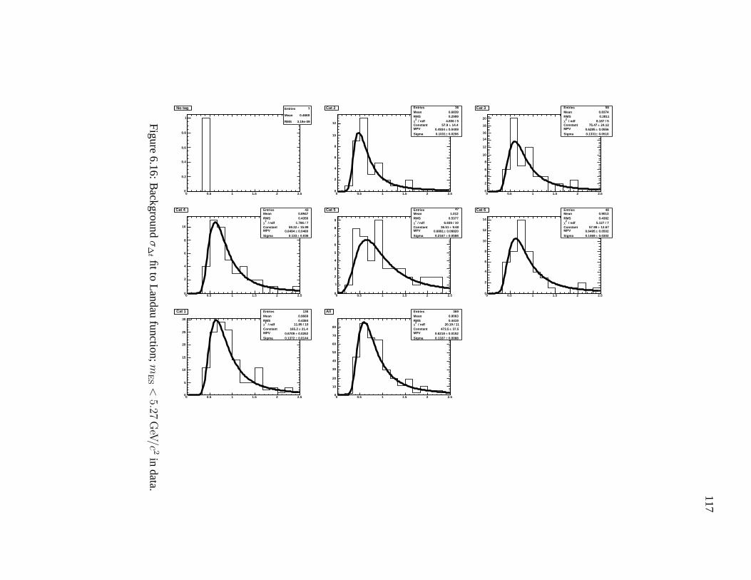
117

0 0.5 1 1.5 2 2.50

0.2

0.4

0.6

0.8

1

No tag Entries 1

Mean 0.4669

RMS 3.19e-09

No tag

0 0.5 1 1.5 2 2.50

2

4

6

8

10

12


/ ndf 2χ 4.806 / 5


Cat 2

0 0.5 1 1.5 2 2.50

2

4

6

8

10

12

14

16

18

20


/ ndf 2χ 8.187 / 5


Cat 3

0 0.5 1 1.5 2 2.50

2

4

6

8

10


/ ndf 2χ 1.786 / 7


Cat 4

0 0.5 1 1.5 2 2.50

1

2

3

4

5

6

7

8

9


/ ndf 2χ 6.939 / 10


Cat 5

0 0.5 1 1.5 2 2.50

2

4

6

8

10

12

14


/ ndf 2χ 5.127 / 7


Cat 6

0 0.5 1 1.5 2 2.50

5

10

15

20

25

30


/ ndf 2χ 11.85 / 10


Cat 1

0 0.5 1 1.5 2 2.50

10

20

30

40

50

60

70

80

All Entries 369Mean 0.9063RMS 0.4419

/ ndf 2χ 20.19 / 11


All

Figure6.16:

Background

σ∆t fitto

Landau

function;m

ES<

5.27G

eV/c

2in

data.

118

6.4 Toy MC Validations

Monte Carlo experiments are generated with parameters fitted from signal MC and the back-

ground data sample, mES < 5.27GeV/c2. To test the sensitivity to the asymmetries we generate

S3K0S

and C3K0S

, randomly, in the physical region S2 + C2 < 1 and do some diagnostic checks.

Signal and background yields are generated using Poisson distributions with signal and background

parameters centered at the values we found in the Run1-4 fit (Nsig = 89 and Nbkg = 439). The

σ∆t distributions used are shown in section 6.3.1. Figure 6.17 shows the fitted values of the asym-

metries and the mean of the pull distributions as a function of the corresponding generated values.

These results provide a quantitative measure of the linearity of the fit procedure. A linear fit to the

correlation between generated and measured values for S and C have slopes within 2σ of unity. We

use the observed correlation to correct the measured values of S and C .

The mean values for pull distributions all lie within 2σ of zero, while a fit with a straight line

exhibits a slope consistent with zero. The standard deviations of the pull distribution shown in

fig. 6.18 are typically slightly larger than one. We suspect this is due to some fraction of the fits

giving unphysical results. This happens when the random values of S and C are close to unity.

About 18% of fits lie in the unphysical region S2 + C2 = 1 and 0.6% are unphysical and lie 3σ

away from one, or are highly unphysical. The widths of the S and C pull distributions shown in

fig. 6.19 for an ensemble of experiments generated with random physical values for S and C are

larger than one as expected.

With a cut of |S| < 1.15 and |C| < 1.15 for the S pull and |S| < 1.2 and |C| < 1.2 for the C

pull, the distributions have a mean which is one σ away from zero (see figure 6.20). Therefore our

theory about the unphysical fits making the pulls larger is valid.

6.4.1 Validation of Fit on Embedded Toy Monte Carlo Experiments

We also do embedded Toy MC studies where a random subset of signal MC events is mixed

with background events generated with the Toy MC technique. These studies are intended to show

whether the correlations in the variables in the maximum likelihood fit bias our results. As we saw

in section 6.2 mES and ∆E are the two variable with largest correlation.

Fits are performed to an ensemble of embedded Toy MC experiments with the correct proportion

of background events observed in data. Table 6.4.1 shows the mean values and standard deviations

from the ensembles generated with four different combinations of values for S and C .

We also do fits with the number of signal and background events set to the value obtained from a

fit to the data. Likewise, fits are performed with the background fixed to zero. We compare the set of

119

fits for the same random combination of signal MC events to determine whether the CP information

is diluted by adding background. We see no evidence of any dilutions. The residuals of these fits

are shown in Figs. 6.21 and 6.22.

Since we have a small sample of MC events, we run the risk of oversampling and amplifying

slight biases after scaling to larger samples. If there is a small bias in the MC sample we will arti-

ficially make the bias larger if we reuse events selected randomly for these tests. We can overcome

this by first fitting a large sample of MC events as shown earlier in table 6.4.1 to check that no bias

is introduced from correlations in the signal events. Then by comparing samples with and without

background events as was shown in figures 6.21 and 6.22 we can determine if the CP information

is diluted by the addition of the background events.

Generated S-1 -0.8 -0.6 -0.4 -0.2 -0 0.2 0.4 0.6 0.8 1

Fit

ted

S

-1.5

-1

-0.5

0

0.5

1

1.5

S Linearity Plot / ndf 2χ 24.68 / 38

p0 0.009001± 0.006082

p1 0.0227± 0.9797

S Linearity Plot

Generated C-1 -0.8 -0.6 -0.4 -0.2 -0 0.2 0.4 0.6 0.8 1

Fit

ted

C

-1.5

-1

-0.5

0

0.5

1

1.5

C Linearity Plot / ndf 2χ 33.54 / 38

p0 0.005781± 0.002434

p1 0.0152± 0.9448

C Linearity Plot

Generated S-1 -0.8 -0.6 -0.4 -0.2 -0 0.2 0.4 0.6 0.8 1

S p

ull

mea

n

-1

-0.8

-0.6

-0.4

-0.2

-0

0.2

0.4

0.6

0.8

1

S Pull Plot / ndf 2χ 28.8 / 38

p0 0.022868± 0.007669

p1 0.057892± 0.006856

S Pull Plot

Generated C-1 -0.8 -0.6 -0.4 -0.2 -0 0.2 0.4 0.6 0.8 1

C p

ull

mea

n

-1

-0.8

-0.6

-0.4

-0.2

-0

0.2

0.4

0.6

0.8

1

C Pull Plot / ndf 2χ 31.18 / 38

p0 0.022110± 0.005262

p1 0.0599± -0.1194

C Pull Plot

Figure 6.17: Fitted S and C versus their generated values in Toy Monte Carlo studies (first

row). Mean of the pull distribution versus generated value in Toy Monte Carlo studies

(second row). Pull is defined as (xfitted − xgenerated)/xerror where is x is the variable in

question and xerror is the error on x determined from the fit. The red line is the expectation

if the measured result from the fit agrees on average with the generated value and the black

line is the result of a fit to a linear function of generated values.

120

Generated S-1 -0.8 -0.6 -0.4 -0.2 -0 0.2 0.4 0.6 0.8 1

0.6

0.8

1

1.2

1.4

1.6

1.8

2

S Width Pull Plot Entries 40Mean 0.01182RMS 0.5533

/ ndf 2χ 84.22 / 38p0 0.0144± 0.9541 p1 0.03333± 0.03765

S Width Pull Plot

Generated C-1 -0.8 -0.6 -0.4 -0.2 -0 0.2 0.4 0.6 0.8 1

0.6

0.8

1

1.2

1.4

1.6

1.8

2

C Width Pull Plot Entries 40Mean -0.05074RMS 0.5719

/ ndf 2χ 53.53 / 38p0 0.015± 1.031 p1 0.0388± -0.1116

C Width Pull Plot

Figure 6.18: Standard deviation of the pull distribution for S and C from Toy Monte Carlo

studies with a cut of |S| < 1.1 and |C| < 1.1. Pull is defined as (xfitted − xgenerated)/xerror

where is x is the variable in question. The red line is the expectation if the errors from the

fit are correct and the black line is the result of a fit to a linear function of generated value.

Entries 2202Mean 0.02183

RMS 1.18 / ndf 2χ 43.91 / 34

Constant 5.1± 182.3 Mean 0.02447± 0.01913

Sigma 0.020± 1.133

-6 -4 -2 0 2 4 60

20

40

60

80

100

120

140

160

180

200

220


RMS 1.18 / ndf 2χ 43.91 / 34

Constant 5.1± 182.3 Mean 0.02447± 0.01913

Sigma 0.020± 1.133

S Pull Entries 2202Mean -0.007011RMS 1.128

/ ndf 2χ 51.66 / 37Constant 5.4± 196.4 Mean 0.0227± -0.0331 Sigma 0.018± 1.048

-6 -4 -2 0 2 4 60

20

40

60

80

100

120

140

160

180

200

220

Entries 2202Mean -0.007011RMS 1.128

/ ndf 2χ 51.66 / 37Constant 5.4± 196.4 Mean 0.0227± -0.0331 Sigma 0.018± 1.048

C Pull

Figure 6.19: S3K0S

andC3K0S

pull distributions from Toy MC studies with random generated

values for S and C.Entries 2011Mean 0.00486

RMS 1.03 / ndf 2χ 29.13 / 26

Constant 5.2± 187.2 Mean 0.02299± 0.01441

Sigma 0.017± 1.015

-6 -4 -2 0 2 4 60

20

40

60

80

100

120

140

160

180

200

220


RMS 1.03 / ndf 2χ 29.13 / 26

Constant 5.2± 187.2 Mean 0.02299± 0.01441

Sigma 0.017± 1.015

S Pull Entries 2042Mean -0.007215

RMS 1.053 / ndf 2χ 30.26 / 31

Constant 5.3± 189.8 Mean 0.02268± -0.01772

Sigma 0.017± 1.015

-6 -4 -2 0 2 4 60

20

40

60

80

100

120

140

160

180

200

Entries 2042Mean -0.007215

RMS 1.053 / ndf 2χ 30.26 / 31

Constant 5.3± 189.8 Mean 0.02268± -0.01772

Sigma 0.017± 1.015

S Pull

Figure 6.20: S3K0S

andC3K0S

pull distributions from Toy MC studies with a cut of |S| < 1.15

and |C| < 1.15 for the S pull and a cut of |S| < 1.2 and |C| < 1.2 for the C pull.

121

Table 6.11: Fits to ensembles of Toy MC generated background events embedded with full

MC signal events for different values of S and C.

Parameter S = C = 0.0 S = 0.7C = 0.0 S = 0.8C = 0.2 S = 0.5C = 0.5

C3K0S

0.0018 ± 0.0160 0.0025 ± 0.0203 0.1990 ± 0.0207 0.5169 ± 0.0190

S3K0S

0.0366 ± 0.0237 0.7334 ± 0.0278 0.8012 ± 0.0279 0.5146 ± 0.0286

Table 6.12: Summary of mean residuals of S3K0S

and C3K0S

; Difference between embedded

Toy MC fits with and without background

Parameter S=C=0.0 S=0.7 C=0.0 S=0.8 C=0.2 S=0.5 C=0.5

δC3K0S

0.0004 0.0012 0.0041 -0.0007

δS3K0S

-0.0066 -0.0038 -0.0161 -0.0097

122

-0.5 -0.4 -0.3 -0.2 -0.1 -0 0.1 0.2 0.3 0.4 0.50

10

20

30

40

50

S Resid Entries 884

Mean -0.006389

RMS 0.1141

/ ndf 2χ 91.16 / 72

Constant 1.69± 32.66

Mean 0.003463± -0.006597

Sigma 0.00362± 0.09641

S Resid

-0.5 -0.4 -0.3 -0.2 -0.1 -0 0.1 0.2 0.3 0.4 0.50

5

10

15

20

25

30

35

40

45

C Resid Entries 884

Mean -0.001922

RMS 0.09974

/ ndf 2χ 60.59 / 52


Mean 0.0034319± 0.0003955

Sigma 0.00278± 0.09513

C Resid

-0.5 -0.4 -0.3 -0.2 -0.1 -0 0.1 0.2 0.3 0.4 0.50

5

10

15

20

25

30

35

S Resid Entries 906

Mean -0.006281

RMS 0.117

/ ndf 2χ 57.34 / 68


Mean 0.003776± -0.003795

Sigma 0.003± 0.108

S Resid

-0.5 -0.4 -0.3 -0.2 -0.1 -0 0.1 0.2 0.3 0.4 0.50

5

10

15

20

25

30

35

40

45

C Resid Entries 906

Mean 0.002621

RMS 0.1037

/ ndf 2χ 53.16 / 61


Mean 0.003459± 0.001168

Sigma 0.00293± 0.09813

C Resid

Figure 6.21: Residual distributions of S3K0S

and C3K0S

; Difference between embedded Toy

MC fits with and without background events. Generated value of S=0.7 and C=0.0 for first

row and S=0.0 and C=0.0 for second row.

123

-0.5 -0.4 -0.3 -0.2 -0.1 -0 0.1 0.2 0.3 0.4 0.50

10

20

30

40

50

S Resid Entries 890

Mean -0.008693

RMS 0.1238

/ ndf 2χ 132.2 / 76

Constant 1.7± 32.6

Mean 0.00354± -0.01612

Sigma 0.0034± 0.0914

S Resid

-0.5 -0.4 -0.3 -0.2 -0.1 -0 0.1 0.2 0.3 0.4 0.50

10

20

30

40

50

C Resid Entries 890

Mean 0.007518

RMS 0.09784

/ ndf 2χ 66.71 / 54


Mean 0.003295± 0.004095

Sigma 0.00316± 0.09108

C Resid

-0.5 -0.4 -0.3 -0.2 -0.1 -0 0.1 0.2 0.3 0.4 0.50

5

10

15

20

25

30

35

40

S Resid Entries 896

Mean -0.01045

RMS 0.1232

/ ndf 2χ 73.49 / 71


Mean 0.003866± -0.009722

Sigma 0.0035± 0.1088

S Resid

-0.5 -0.4 -0.3 -0.2 -0.1 -0 0.1 0.2 0.3 0.4 0.50

10

20

30

40

50

C Resid Entries 896

Mean 0.0004895

RMS 0.1039

/ ndf 2χ 63.09 / 60


Mean 0.0034690± -0.0006971

Sigma 0.00282± 0.09803

C Resid

Figure 6.22: Residual distributions of S3K0S

and C3K0S

; Difference between embedded Toy

MC fits with and without background. Generated value of S=0.8 and C=0.2 for first row

and S=0.5 and C=0.5 for second row.

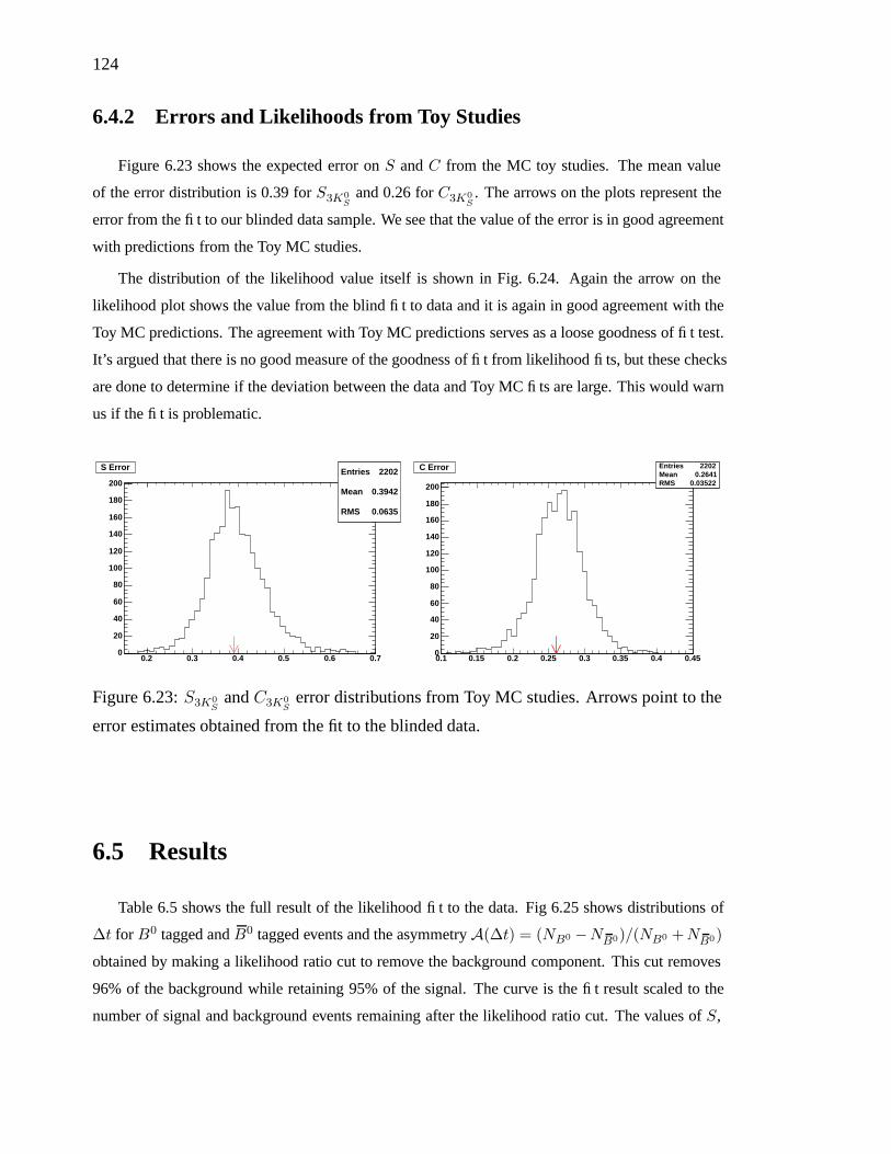
124

6.4.2 Errors and Likelihoods from Toy Studies

Figure 6.23 shows the expected error on S and C from the MC toy studies. The mean value

of the error distribution is 0.39 for S3K0S

and 0.26 for C3K0S

. The arrows on the plots represent the

error from the fit to our blinded data sample. We see that the value of the error is in good agreement

with predictions from the Toy MC studies.

The distribution of the likelihood value itself is shown in Fig. 6.24. Again the arrow on the

likelihood plot shows the value from the blind fit to data and it is again in good agreement with the

Toy MC predictions. The agreement with Toy MC predictions serves as a loose goodness of fit test.

It’s argued that there is no good measure of the goodness of fit from likelihood fits, but these checks

are done to determine if the deviation between the data and Toy MC fits are large. This would warn

us if the fit is problematic.

Entries 2202

Mean 0.3942

RMS 0.0635

0.2 0.3 0.4 0.5 0.6 0.70

20

40

60

80

100

120

140

160

180

200Entries 2202

Mean 0.3942

RMS 0.0635

S Error Entries 2202Mean 0.2641RMS 0.03522

0.1 0.15 0.2 0.25 0.3 0.35 0.4 0.450

20

40

60

80

100

120

140

160

180

200

Entries 2202Mean 0.2641RMS 0.03522

C Error

Figure 6.23: S3K0S

and C3K0S

error distributions from Toy MC studies. Arrows point to the

error estimates obtained from the fit to the blinded data.

6.5 Results

Table 6.5 shows the full result of the likelihood fit to the data. Fig 6.25 shows distributions of

∆t for B0 tagged and B0 tagged events and the asymmetry A(∆t) = (NB0 −NB0)/(NB0 +NB0)

obtained by making a likelihood ratio cut to remove the background component. This cut removes

96% of the background while retaining 95% of the signal. The curve is the fit result scaled to the

number of signal and background events remaining after the likelihood ratio cut. The values of S,

125

C , and Nsig determined from the fit with asymmetric errors are

S = −0.71+0.38−0.32

C = −0.34+0.28−0.25

Nsig = 86.7+10.5−9.8 .

Fixing C = 0, which is the Standard Model expectation, we obtain sin 2βeff = −S = 0.79+0.29−0.36 .

Figure 6.26 shows the maximum likelihood value as a function of S and C . This shows that our

results are indeed the minimum of the likelihood function as expected.

The distribution of per event weights and event weights versus ∆t are shown in fig. 6.27. The

event weight is the log likelihood contribution for the individual event. We see that the events with

a large -log likelihood are ones with large ∆t in data. This trend is also observed in Toy MC events,

as shown in 6.28. The Toy MC results are obtained by generating a sample 20 times larger than

data, but with the observed ratio of background to signal. An overlay of the data and Toy MC events

also shows good agreement. This is shown in fig. 6.29 and gives us confidence in our modeling of

data events.

Entries 2202Mean -1269RMS 85.73

-1700 -1600 -1500 -1400 -1300 -1200 -1100 -10000

10

20

30

40

50

60

70

80

Entries 2202Mean -1269RMS 85.73

NLL

Figure 6.24: Log(likelihood) distribution from Toy MC studies. Arrow points to result

from blind fit.

126

6.5.1 sPlots

Figures 6.30- 6.33 show sP lots of mES, ∆E, F , and ∆t [31]. These figures are made by

first omitting the projection variable, the variable being plotted, and fitting the remaining variables,

to estimate signal and background yields. For each event, a weight to be signal or background is

derived according to these fit results and the probability distributions in the restricted set of variables.

Using these weights, the data is then plotted in the projection variable. The curves show the results

of the fit to the restricted set of variables for comparison. Note that the final results are based on a

fit to all variables.

T (ps)∆-6 -4 -2 0 2 4 6

0

5

10

15

T (ps)∆-6 -4 -2 0 2 4 6

0

5

10

15(a)0B

t (ps)∆-6 -4 -2 0 2 4 6

0

5

10

t (ps)∆-6 -4 -2 0 2 4 6

0

5

10 (b)0B

t (ps)∆-6 -4 -2 0 2 4 6

-1

-0.5

0

0.5

1

t (ps)∆-6 -4 -2 0 2 4 6

-1

-0.5

0

0.5

1 (c)

Eve

nts

/ 1.5

ps

Asy

mm

etry

Figure 6.25: Distributions of ∆t for background subtracted events for Btag tagged as (a)

B0 or (b) B0, and (c) the asymmetry A(∆t). We use a likelihood ratio cut that removes

96% of the background while retaining 95% of the signal. The curve is the scaled fit result.

127

6.6 Systematic Uncertainties and Cross Checks

The errors on this measurement are expected to be dominated by the statistical error, but the

systematic error must be determined and cross checks on the data must be performed to insure con-

sistency in the data sample. Section 6.6.1 explains and shows estimates of the sources of systematic

uncertainties on S and C . Section 6.6.2 shows the list of cross checks performed on the data sample.

6.6.1 Systematic Uncertainties

This section details the systematic uncertainties on the asymmetries S and C which are listed

in table 6.14. The main source of uncertainty arises from the PDF uncertainty. The uncertainty on

the PDF parameters arises from the error from the fit to the data sample. In general to determine

the uncertainty on S and C data is refit changing a parameter in the fit. Other ways to estimate an

uncertainty is to use MC control samples as is done for the SVT alignment and tag side interference

S-1 -0.8 -0.6 -0.4 -0.2 -0 0.2 0.4 0.6 0.8 1

Lo

g L

∆

0

2

4

6

8

10

Log Likelihood vs S∆

C-1 -0.8 -0.6 -0.4 -0.2 -0 0.2 0.4 0.6 0.8 1

Lo

g L

∆

0

2

4

6

8

10

Log L vs C∆

Figure 6.26: ∆ Likelihood functions for S and C from fit to data.


0 1 2 3 4 5 6 7 8 9 100

5

10

15

20

25


Event -Log(Likelihood)

0 1 2 3 4 5 6 7 8 9 10

t(ps

)∆

−20

−15

−10

−5

0

5

10

15

20

Entries 528Mean x 2.546Mean y −0.1733RMS x 1.468RMS y 2.243


t vs Event −Log(Likelihood)∆

Figure 6.27: Distribution of -log(likelihood) and correlation between -log(likelihood) and

∆t for data events.

128

systematic uncertainties. Also any fit bias determined from the Toy MC events is added as a system-

atic uncertainty. Other systematic uncertainties are determined by a comparison of signal and MC

events as for the vertexing method and the ∆t resolution function uncertainties. There is no well

defined procedure for determining sources of systematic uncertainties, therefore potential sources

of uncertainties have to be considered and tested.

Systematic Uncertainties from PDF parametrization

Tables A- A in Appendix A provide a detailed account of the estimated systematic uncertainties

from varying the signal PDF parameters in the fit by their error. These errors are mostly statistical in

nature. The exceptions are ∆m and τB0 whose values are varied by their error in the PDG [13]. The

PDF systematics are summarized in table 6.14 lines 1-7 of the PDF section, the top portion separated


0 2 4 6 8 10 120

100

200

300

400

500

600


Event -Log(Likelihood) Toy Events

∆t(

ps)

0 2 4 6 8 10 12−20

−15

−10

−5

0

5

10

15

20



t vs Event −Log(Likelihood) Toy Events∆

Figure 6.28: Distribution of -log(likelihood) and correlation between -log(likelihood) and

∆t for a Toy MC sample of events.


0 1 2 3 4 5 6 7 8 9 100

0.02

0.04

0.06

0.08

0.1




Event -Log(Likelihood) Data and Toy Entries 528Mean 2.546RMS 1.468

0 1 2 3 4 5 6 7 8 9 10

-310

-210

-110


Event -Log(Likelihood) Data and Toy Entries 12877Mean 2.576RMS 1.458

Figure 6.29: Distribution of -log(likelihood) for data events (points with error bars) and

Toy MC (overlaid histogram) on a linear (left) and log scale (right).

129

by horizontal line. The systematic uncertainty, ∆S or ∆C , is estimated from the difference between

the nominal fit and the fit where the PDF parameter in question is varied up and down by the error.

The sign of ∆S or ∆C is shown in the table. If both values are positive (negative), the greater

(lesser) of the two is taken for the +(-) category and the -(+) category is set to zero. The other

systematics in the PDF category are obtained from floating µ SmES

and µS∆E to make sure the MC

values are similar to data values and therefore do not bias our results on S and C . The total sum for

the PDF systematics are 0.0254 for S and 0.0263 for C .

[GeV]ESm5.22 5.23 5.24 5.25 5.26 5.27 5.28 5.29 5.3

Eve

nts

/ (

0.00

16 )

0

5

10

15

20

25


[GeV]ESm5.22 5.23 5.24 5.25 5.26 5.27 5.28 5.29 5.3

Eve

nts

/ (

0.00

16 )

0

5

10

15

20

25


[GeV]ESm5.22 5.23 5.24 5.25 5.26 5.27 5.28 5.29 5.3

Eve

nts

/ (

0.00

16 )

0

2

4

6

8

10

12

14

16

18

20

22

24


[GeV]ESm5.22 5.23 5.24 5.25 5.26 5.27 5.28 5.29 5.3

Eve

nts

/ (

0.00

16 )

0

2

4

6

8

10

12

14

16

18

20

22

24


Figure 6.30: sPlot of signal (left) and background (right) mES.

E [GeV]∆-0.1 -0.05 0 0.05 0.1

Eve

nts

/ (

0.01

6 )

0

5

10

15

20

25

30

35


E [GeV]∆-0.1 -0.05 0 0.05 0.1

Eve

nts

/ (

0.01

6 )

0

5

10

15

20

25

30

35


E [GeV]∆-0.1 -0.05 0 0.05 0.1

Eve

nts

/ (

0.01

6 )

0

10

20

30

40

50


E [GeV]∆-0.1 -0.05 0 0.05 0.1

Eve

nts

/ (

0.01

6 )

0

10

20

30

40

50


Figure 6.31: sPlot of signal (left) and background (right) ∆E.

130

SVT Alignment and Boost Uncertainties

We rely on the precision of the SVT for reconstructing decay vertices and for tracking charged

particles in the detector. The precision of determining the position of a charged particle in the SVT

however is only as good as our knowledge of the relative position of the silicon wafers. Determining

the position of the wafers and strips relative to their nominal position is known as the local SVT

alignment.

The internal alignment of SVT wafers is determined by comparing measured versus projected

Fisher-5 -4 -3 -2 -1 0 1 2 3 4 5

Eve

nts

/ (

0.90

9091

)

0

10

20

30

40

50


Fisher-5 -4 -3 -2 -1 0 1 2 3 4 5

Eve

nts

/ (

0.90

9091

)

0

10

20

30

40

50


Fisher-5 -4 -3 -2 -1 0 1 2 3 4 5

Eve

nts

/ (

0.90

9091

)

0

50

100

150

200

250


Fisher-5 -4 -3 -2 -1 0 1 2 3 4 5

Eve

nts

/ (

0.90

9091

)

0

50

100

150

200

250


Figure 6.32: sPlot of signal (left) and background (right) F .

T [ps]∆-20 -15 -10 -5 0 5 10 15 20

Eve

nts

/ (

0.8

)

0

5

10

15

20


T [ps]∆-20 -15 -10 -5 0 5 10 15 20

Eve

nts

/ (

0.8

)

0

5

10

15

20


T [ps]∆-20 -15 -10 -5 0 5 10 15 20

Eve

nts

/ (

0.8

)

0

20

40

60

80

100

120

140


T [ps]∆-20 -15 -10 -5 0 5 10 15 20

Eve

nts

/ (

0.8

)

0

20

40

60

80

100

120

140


Figure 6.33: sPlot of signal (left) and background (right) ∆t.

131

positions of tracks obtained from the process e+e− → µ+µ− for studying the parameters d0, z0,

and φ0 defined in section 3.4.1. The position of the wafers is expressed in terms of a rotation and

translation with respect to the nominal alignment.

Systematic uncertainties from residual uncertainties in the SVT local alignment are determined

from simulated MC events. Several misalignment scenarios are introduced in the reconstruction

of the MC, which is normally reconstructed with the nominal alignment, to determine systematic

effects.

We also take into account the uncertainty of the radius-dependent z shift of entire layers which

is equivalent to having an uncertainty in the boost, βγ. This uncertainty is computed from MC

events in the same fashion as the SVT misalignments.

We fit a Monte Carlo sample reconstructed in refit mode with four different misalignment sce-

narios and one boost uncertainty file [32]. Refit mode means the tracks are refit, or reconstructed

again, instead of being taken from a stored nominal reconstruction in the database called cache

mode. We also reconstruct events without misalignment in the refit mode to make sure any differ-

ences are not coming from the reconstruction method.

For each misalignment scenario we compare the sample without misalignment (‘nominal’) with

the sample with misalignment. To reduce the impact of statistical fluctuations due to events entering

or leaving the selection, we select only events that are common in the nominal and the misaligned

sample. The errors are added in quadrature for the total systematic uncertainty. The variation if S

and C for each misalignment file and the total systematic uncertainty are shown in table 6.6.1.

Vertexing and Resolution Function

To determine if there is a difference in our vertexing method versus the nominal vertexing

method used by most other time dependent analyses at BABAR, we fit our MC sample with the

resolution function parameters taken from B0 → K0SK

0SK

0S MC and Dc, ∆Dc, µc, and εc taken

from the MC Bflav sample. The difference between this fit and the nominal fit, with all parameters

taken from the B0 → K0SK

0SK

0S , is assigned as the systematic error. This is done on a MC sample

with S = 0.8 and C = 0.2. We find a variation of 0.020 for S and 0.022 for C .

To determine a systematic error on the resolution function, we first compare the resolution func-

tions of B0 → K0SK

0SK

0S MC to the Bflav MC values and determine scale and offsets differences.

We then scale or shift the Bflav data resolution function values according to the differences seen

between the two MC samples. The bias values are shifted and the other parameters, σcore, fout, and

ftail are scaled. The difference in S and C from the nominal fit in data is taken as a systematic error.

These values are 0.017 for both S and C .

132

Background Tagging Asymmetry

We set the background tagging asymmetry parameters to zero since in the fit we see that most

tagging categories have values which are consistent with zero. It is likely that their deviation from

zero is just a statistical fluctuation. There is also no mechanism where an asymmetry in the back-

ground could be produced so we expect those values to be zero. This gives an uncertainty in S of

0.007 and in C of 0.022.

Embedded Toy MC Bias/Correlations in Fit Parameter

Correlations in the fit parameters would effect signal and background yields and therefore vary

the values of S and C . We assign a systematic error for the correlation between the fit parameters by

taking the largest residual from Table 6.4.1. This table shows the mean of the residuals of S and C

when fitting signal MC events only and when adding generated background events. These residuals

are a measure of uncertainty of S and C from correlations. For C the largest residual is 0.004 and

for S it’s 0.016.

Tag Side Interference

Interference between CKM-favored b→ cud and doubly-CKM suppressed b→ ucd amplitudes

in final states used for B flavor tagging gives deviations from the standard time evolution assumed

in CP violation measurements [33]. For example a tag B meson may be observed in the D+π−

mode and generate a K− tag from the D+. The dominant amplitude contribution is from the B0

decay (b → cud), but a suppressed amplitude from the B0 decay (b → ucd) cannot be ruled out.

These two amplitudes will interfere with a relative weak phase of γ and a relative strong phase

of δ′

from final-state interactions. A rough estimate of the relative size of these amplitudes is

r′ ∼ |V ∗

ubVcd/VcbV∗ud| = 0.02. Events which decay semileptonically are immune to this effect.

Using equation (31) and (32) in [33]:

Cfit = C0[1 + 2r′cos δ

′G cos(2β + γ) − S0 sin(2β + γ)] − 2r′sin δ

′S0 cos(2β + γ)

+ G sin(2β + γ) (6.5)

Sfit = S0[1 + 2r′cos δ

′G cos(2β + γ)] + 2r′sin δ

′C0 cos(2β + γ) (6.6)

where G ≡ 2ReλCP/(|λCP |2 + 1) which in the standard model would give G ≡ − cos(2β) since

λ = −e2iβ , we can determine the deviation of S and C from the nominal value. We generate values

of γ[39◦, 80◦], δ′[0, 2π], and r

′[0.00, 0.04], and 2β = 47.7◦ and determine the one sigma deviation

133

of the Cfit and Sfit distributions which we define as δC and δS respectively. We can then use the

relation:

δSDCSD =∑

i

εNSL,iDNSL,i

〈Di〉QiδS (6.7)

δCDCSD =∑

i

εNSL,iDNSL,i

〈Di〉QiδC (6.8)

where εNSL,i and DNSL,i are the efficiency and dilutions respectively of events which decayed non-

semileptonically at the MC truth level and 〈Di〉 and Qi are the average dilutions and quality factor

respectively for all events for tagging category i. The value of∑

i εNSL,iDNSL,i

〈Di〉 Qi = 0.4965. We

then input the values of S and C that are determined from our fit and vary them by one sigma. The

values which give the largest deviations are taken as the systematic uncertainty. The uncertainty on

S is determined to be 0.008 and for C to be 0.015.

6.6.2 Cross Checks

To insure consistency of the data sample we perform the cross checks which are shown in this

section.

Floating B0 Lifetime

In the nominal fit the B0 lifetime is fixed to 1.537 ± 0.015 [13]. Redoing the nominal fit for

extracting S and C and floating B 0 lifetime gives τB0 = 1.771± 0.231 which is consistent with the

world average which is used in the nominal fit. The values of S and C change by +0.022 and -0.016

respectively from the nominal value, however these numbers are just quoted to access the impact on

the asymmetries and are not used as systematic errors.

Splitting Runs 1-3 and Run4

In order to check the consistency of subsamples of the full data set, we compare fits to run 1-3

versus run4. Given the limited background statistics in the subsamples, we are unable to determine

background parameters independently. Instead we fix all fit variables to the values taken from the

full sample with the exception of yields and the C and S time-dependent coefficients. Table 6.6.2

shows the blind results, since these checks were done before unblinding our results, on the asym-

metries, the yields, purity, Nsig/Nbkg, and the deviations of S and C in the subsamples from the

full run 1-4 fit. The purity is calculated by Purity=Nsig/σ(Nsig)2. We see that the asymmetries and

yields are consistent across the samples.

134

BC Vertexing Method Versus TreeFitter

In order to determine if the TreeFitter method has the same performance as the BC vertexing

method which was tested in great detail in the B0 →K0S π

0 analysis, we fit signal MC events using

∆t and σ∆t from the BC vertex method. This test will validate that the two methods are similar and

there are no unexpected biases between the two. Table 6.6.2 shows fits to two MC samples with

and without an asymmetry. We see slight variations in the measured values of S and C which are

within statistics of the sample. The same events are used in the fit with different vertexing methods

to avoid any statistical fluctuations in the central value.

B Background

A study has been performed where an additional uncorrelated B background component is

added to the background sample. From our study of BB MC events, we demonstrated that most of

the B background is evenly distributed in mES and ∆E. Enlarging the B background component

three-fold from the expected level of 4 events we find that when the additional events have zero

lifetime, the change in S is negligible while C changes by 0.004. With a non-zero lifetime the

change in S and C are negligible since it does not pick up any B background component from this

fit. These events are absorbed in the continuum background component. We conclude that the effect

of an additional background component is negligible.

Branching Fraction Check

Using our measured signal yield we estimate a branching fraction (BF) of (6.8 ± 0.8)x10−6

for B0 → K0SK

0SK

0S . Note that this yield is after ∆t and σ∆t selection requirements described in

section 6.3. We’ve quoted a BF just as a consistency check with the BF analysis. This result is

consistent with the BF analysis measurement of (6.9± 0.8 ± 0.8)x10−6 [34]. The slight deviations

come from possible data/MC differences in efficiency when making selection requirements on ∆t

and σ∆t.

135

Table 6.13: Result of fit to full dataset showing values of all parameters floated in the fit.

Parameter Value

NB 441.3 ± 21.4

NS 86.7 ± 10.1

P1 -0.649 ± 0.657

P2 -7.43 ± 9.91

bcore -0.0305 ± 0.0778

score 1.1801 ± 0.0758

fout 0.0205 ± 0.0104

ftail 0.1578 ± 0.0461

µCat2 0.03 ± 0.149

µCat3 -0.171 ± 0.124

µCat4 -0.015 ± 0.145

µCat5 -0.259 ± 0.121

µCat6 -0.242 ± 0.131

btail 0.007 ± 0.471

µBF 0.6253 ± 0.0678

σBLF 0.5327 ± 0.0441

σBRF 0.6446 ± 0.0445

ξ -11.47 ± 6.99

εCat2 0.1044 ± 0.0148

εCat3 0.1482 ± 0.0172

εCat4 0.1106 ± 0.0152

εCat5 0.1468 ± 0.017

εCat6 0.1271 ± 0.016

C3K0S

-0.338 ± 0.265

S3K0S

-0.707± 0.362

136

Table 6.14: Breakdown of all contributions to the systematic uncertainty on S and C.

∆S ∆C

(+) (−) (+) (−)

mES PDf 0.0021 0.0038 0.0009 0.0010

∆E PDF 0.0008 0.0034 0.0017 0.0019

F PDF 0.0032 0.0057 0.0017 0.0024

resolution function 0.0097 0.0128 0.0061 0.0060

D and ∆D 0.0105 0.0150 0.0080 0.0082

εtag 0.0003 0.0034 0.0002 0.0008

∆εS 0.0042 0.0080 0.0090 0.0095

µSmESfloat 0.0001 0.0001 0.0000 0.0000

µS∆E float 0.0087 0.0087 0.0020 0.0020

PDF total 0.0254 0.0263

SVT Alignment 0.015 0.008

data/MC RF 0.017 0.017

vertexing method 0.020 0.022

∆εB = 0 0.007 0.022

Embedded fit bias 0.016 0.004

tag side interference 0.008 0.015

Total 0.043 0.047

137

Table 6.15: Effects of SVT misalignment scenarios on measurements of S and C for about

120k MC events. The total systematic error is determined by adding in quadrature the boost

misalignment to the largest value from the time misalignments.

Misalignment ∆S ∆C

Time1 -0.0144 0.0004

Time2 -0.0096 0.0073

Time3 -0.0103 0.0012

Time4 -0.0133 0.0016

Boost -0.0023 0.0016

Total sys 0.0146 0.0075

Table 6.16: Summary of yields and blind asymmetries in data subsamples versus the nom-

inal fit.

Parameter Run1-4 Run 1-3 Run 4

S3K0S

−1.158 ± 0.362 −1.107 ± 0.428 −1.561 ± 0.874

δS3K0S

+0.051 −0.403

C3K0S

−0.790 ± 0.265 −0.648 ± 0.367 −0.953 ± 0.345

δC3K0S

+0.142 −0.163

Nsig 86.7 ± 10.1 52.0 ± 7.7 34.6 ± 6.4

Nbkg 441.3 ± 21.4 259.0 ± 16.3 182.4 ± 13.7

Purity 85.0% 87.7% 84.5%

Nsig/Nbkg 19.6% 20.1% 19.0%

138

Table 6.17: Comparison of fit results with signal MC events using the BC and TreeFitter

vertexing methods

Vertexing Method S = C = 0.5 S = C = 0.0

S C S C

TreeFitter 0.515 ± 0.021 0.499 ± 0.014 0.014 ± 0.017 0.015 ± 0.011

BC 0.525 ± 0.021 0.497 ± 0.014 0.014 ± 0.017 0.014 ± 0.011

Chapter 7

Conclusions

With a data sample of 205 fb−1 amounting to 227 million Υ (4S) → B B decays we measure

CP -violating asymmetries in B0 →K0S K

0S K

0S decays

S3K0S

= −0.71+0.38−0.32 ± 0.04

C3K0S

= −0.34+0.28−0.25 ± 0.05

with 87 ± 10 signal events where the decays of K0S → π+ π− are only considered. This result is

published in Phys. Rev. Lett. [34]. Fixing C = 0, which is the Standard Model expectation, we

obtain sin 2β3K0S

= −S = 0.79+0.29−0.36 ± 0.04.

7.1 Significance of Result

In section 2.5 we showed that the B0 →K0S K

0S K

0S decay is a penguin mode which has a the-

oretically reliable predicted CP asymmetry within the Standard Model, similar to B 0 → φK0S . The

penguin decays are an important experimental probe of new physics beyond the Standard Model. As

shown before a deviation of the sin 2β3K0S

from sin 2βJ/ψK0S

would be an evidence of new physics;

however, our result is quite consistent with SM prediction.

Around the same time the Belle collaboration has also made a measurement of these asymme-

tries: S3K0S

= 1.26 ± 0.68 ± 0.20 and C3K0S

= −0.54 ± 0.34 ± 0.09 [35]. The Belle Collaboration

has much worse uncertainties since their vertexing efficiency and ∆t resolution are much worse than

BABAR’s. The Belle result also includes decays where one K 0S → π0 π0. In a sample of 275 million

Υ (4S) → B B pairs they have 88 ± 13 signal events, therefore they also suffer from lower K 0S

efficiency. This measurement is 2.9σ away from the SM prediction but their uncertainties are quite

139

140

large [35]. The average of the two measurements gave a central value on S of −0.26 ± 0.34 [36]

which is about 1.3σ away from sin 2βJ/ψK0S

.

At the Lepton-Photon Conference which took place in summer of 2005, Belle updated their

results with 386 million Υ (4S) → B B pairs to S = −0.58 ± 0.36 ± 0.08 and C = −0.50 ±0.23 ± 0.06 with 105± 12 signal events [6] [37]. This preliminary measurement has a much better

statistical error which we presume comes from the new silicon vertex tracker installed at Belle since

the additional signal events cannot improve the statistical error about a factor of two. The central

value of S has moved much closer to our result making the two measurements consistent with each

other and also with SM predictions.

7.2 Comparison with other Penguin and Charmonium De-

cays

As seen from fig. 7.1 our result is consistent with both the average from charmonium decays and

the penguin decays. The decay B0 →K0S K

0S K

0S has advantage over decays where the CP content

is not well understood. It is purely CP even whereas other measurements can have a mixture of CP

even and CP odd making it more difficult to interpret results. We also saw in section 2.5 that the SM

prediction for S3K0S

differs from SJ/ψK0S

by ∆S3K0S

= 0.02 when applying the QCD factorization

model [19]. If the measurement of S3K0S

is very different from SJ/ψK0S

this could be evidence for a

new physics phenomenon.

Fig. 7.2 [38] shows the theoretical expectations from QCD factorization for each penguin decay

mode. We see with the exception of the B0 → K0S K

0S K

0S decay the predictions make ∆sin 2β =

sin 2βeff − sin 2βJ/ψK0S> 0 for all other modes. However from figs. 7.1 and 7.3 we see that most

measurements yield ∆sin 2βmeas = sin 2βmeas − sin 2βJ/ψK0S< 0 and the average from penguin

modes, shown as a yellow band, in fig. 7.1 also shows this trend. The opposite sign of the measured

versus expected deviation could be the first hint of new physics in the penguin decays.

Some argue a naive average of the penguin modes can lead to incorrect conclusions since each

mode suffers from a different predicted theoretical uncertainty. Performing a χ2 for each mode

from the predicted theoretical value is a preferred method of comparison. Hence the Heavy Flavor

Averaging Group (HFAG) has been discouraged from performing these naive averages of all the

penguin modes as shown in the yellow band in fig. 7.1.

141

Figure 7.1: Compilation of results of time-dependent CP asymmetries by the Heavy Flavor

Averaging Group (HFAG) from b→ ccs and b→ s penguin decays.

7.3 Future Prospects

BABAR has recently made a preliminary measurement adding decays where one K 0S is allowed

to decay to K0S → π0 π0. Combining those decays with the ones shown in this dissertation the value

of the asymmetries become [39]

S3K0S

= −0.63+0.32−0.28 ± 0.04

C3K0S

= −0.10 ± 0.25 ± 0.05.

This decay includes an additional 41.0+9.2−8.3 signal events which improves the statistical uncer-

tainty. The average of the new Belle measurement with this combined measurement gives a central

value on S of −0.64±0.23 which is consistent with the SM prediction. By summer of 2006 BABAR

142

Figure 7.2: QCD factorization predictions for ∆ sin 2β for different penguin modes. The

gray bar represents upper bounds determined from the range of values from toy studies and

the blue represent upper bounds determined by adding errors in quadrature.

will double their dataset and by summer of 2008 the dataset will be more than five times that pre-

sented in this analysis (see fig. 7.4). Doubling the dataset will make the statistical uncertainty of the

combined result about 0.21 for S and with five times more data the uncertainty will be reduced to

0.13.

Some updates of results presented this summer at the Lepton-Photon Conference shifted the

values of the asymmetries significantly from the winter 2005 results. We saw that the Belle mea-

surement of B0 →K0S K

0S K

0S was greatly improved and the central value shifted to a value consis-

tent with our result as well as with the SM. The value of sin 2β from charmonium modes changed

from 0.726 ± 0.037 to 0.69 ± 0.03 and many other penguin decay measurements changed to move

results closer to sin 2βJ/ψK0S. With BABAR taking data at a steady and improving rate the statistical

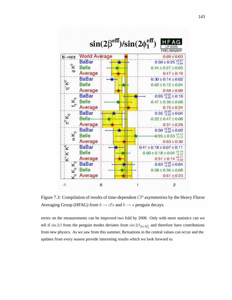
143

Figure 7.3: Compilation of results of time-dependent CP asymmetries by the Heavy Flavor

Averaging Group (HFAG) from b→ ccs and b→ s penguin decays.

errors on the measurements can be improved two fold by 2008. Only with more statistics can we

tell if sin 2β from the penguin modes deviates from sin 2βJ/ψK0S

and therefore have contributions

from new physics. As we saw from this summer, fluctuations in the central values can occur and the

updates from every season provide interesting results which we look forward to.

144

Figure 7.4: Seeman luminosity projection up to Summer of 2008 for both Belle and BABAR.

Appendix A

Systematic Uncertainties from PDF

Variation

This appendix incluces tables for the PDF systematics in Tables A- A.

Table A.1: Change is S and C as a result of varying mES PDF parameters by statistical

error from fit to signal MC.

Parameter Values ∆(S) + ∆(S) - ∆(C) + ∆(C) -

NmES0.7459 ± 0.0926 0.0019 -0.0028 0.0008 -0.0007

αmES2.6896 ± 0.0739 0.0010 -0.0022 0.0001 0.0000

µmES5.2794 ± 0.00003 0.0000 -0.0012 0.0000 -0.0002

σmES0.0026 ± 0.00002 0.0000 -0.0009 0.0005 -0.0006

Total 0.0021 0.0038 0.0009 0.0010

145

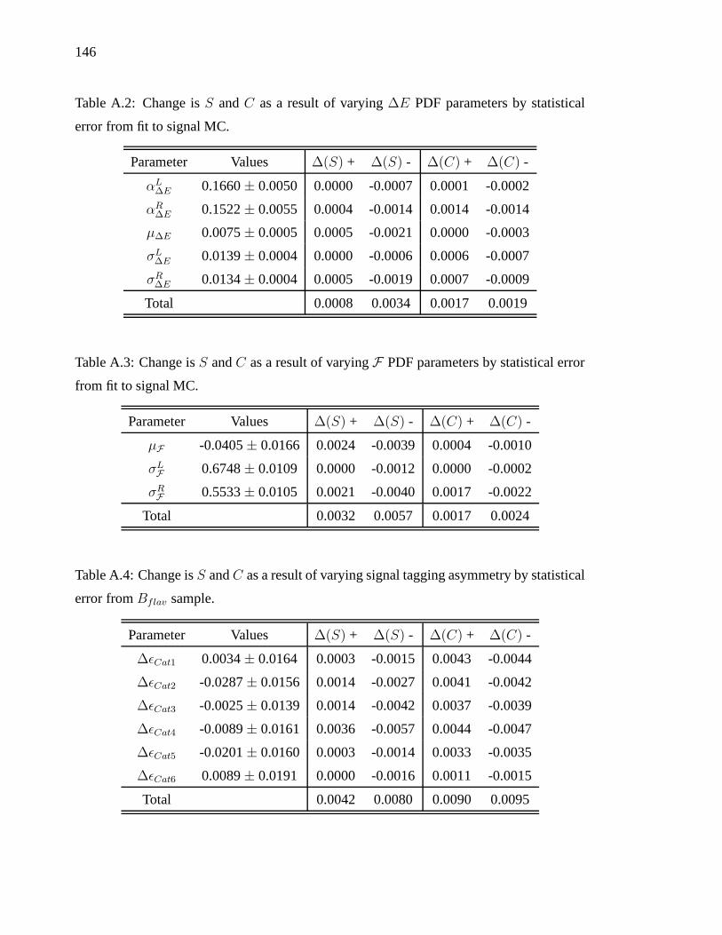
146

Table A.2: Change is S and C as a result of varying ∆E PDF parameters by statistical

error from fit to signal MC.


αL∆E 0.1660 ± 0.0050 0.0000 -0.0007 0.0001 -0.0002

αR∆E 0.1522 ± 0.0055 0.0004 -0.0014 0.0014 -0.0014

µ∆E 0.0075 ± 0.0005 0.0005 -0.0021 0.0000 -0.0003

σL∆E 0.0139 ± 0.0004 0.0000 -0.0006 0.0006 -0.0007

σR∆E 0.0134 ± 0.0004 0.0005 -0.0019 0.0007 -0.0009

Total 0.0008 0.0034 0.0017 0.0019

Table A.3: Change is S and C as a result of varying F PDF parameters by statistical error

from fit to signal MC.


µF -0.0405 ± 0.0166 0.0024 -0.0039 0.0004 -0.0010

σLF 0.6748 ± 0.0109 0.0000 -0.0012 0.0000 -0.0002

σRF 0.5533 ± 0.0105 0.0021 -0.0040 0.0017 -0.0022

Total 0.0032 0.0057 0.0017 0.0024

Table A.4: Change is S and C as a result of varying signal tagging asymmetry by statistical

error from Bflav sample.


∆εCat1 0.0034 ± 0.0164 0.0003 -0.0015 0.0043 -0.0044

∆εCat2 -0.0287 ± 0.0156 0.0014 -0.0027 0.0041 -0.0042

∆εCat3 -0.0025 ± 0.0139 0.0014 -0.0042 0.0037 -0.0039

∆εCat4 -0.0089 ± 0.0161 0.0036 -0.0057 0.0044 -0.0047

∆εCat5 -0.0201 ± 0.0160 0.0003 -0.0014 0.0033 -0.0035

∆εCat6 0.0089 ± 0.0191 0.0000 -0.0016 0.0011 -0.0015

Total 0.0042 0.0080 0.0090 0.0095

147

Table A.5: Change is S and C as a result of varying signal efficiencies by statistical error

from Bflav sample.


εCat1 0.0875 ± 0.0011 0.0000 -0.0013 0.0000 -0.0003

εCat2 0.1089 ± 0.0014 0.0000 -0.0011 0.0001 -0.0003

εCat3 0.1714 ± 0.0017 0.0003 -0.0021 0.0001 -0.0005

εCat4 0.1358 ± 0.0016 0.0002 -0.0012 0.0000 -0.0003

εCat5 0.1469 ± 0.0007 0.0000 -0.0013 0.0000 -0.0003

εCat6 0.0992 ± 0.0012 0.0000 -0.0011 0.0000 -0.0002

Total 0.0003 0.0034 0.0002 0.0008

Table A.6: Change is S and C as a result of varying dilutions and ∆ dilutions by statistical

error from Bflav sample.


DCat1 0.9364 ± 0.0094 0.0000 -0.0023 0.0029 -0.0025

DCat2 0.9001 ± 0.0101 0.0034 -0.0044 0.0017 -0.0024

DCat3 0.6916 ± 0.0111 0.0015 -0.0026 0.0007 -0.0012

DCat4 0.5426 ± 0.0140 0.0063 -0.0077 0.0017 -0.0016

DCat5 0.3377 ± 0.0146 0.0032 -0.0046 0.0001 -0.0013

DCat6 0.1821 ± 0.0183 0.0053 -0.0068 0.0027 -0.0035

∆DCat1 0.0057 ± 0.0180 0.0000 -0.0028 0.0032 -0.0027

∆DCat2 0.0410 ± 0.0190 0.0039 -0.0051 0.0028 -0.0031

∆DCat3 0.0285 ± 0.0190 0.0014 -0.0040 0.0036 -0.0031

∆DCat4 0.0018 ± 0.0227 0.0012 -0.0036 0.0031 -0.0028

∆DCat5 -0.1246 ± 0.0225 0.0000 -0.0017 0.0007 -0.0011

∆DCat6 -0.0843 ± 0.0272 0.0000 -0.0016 0.0007 -0.0009

Total 0.0105 0.0150 0.0080 0.0082

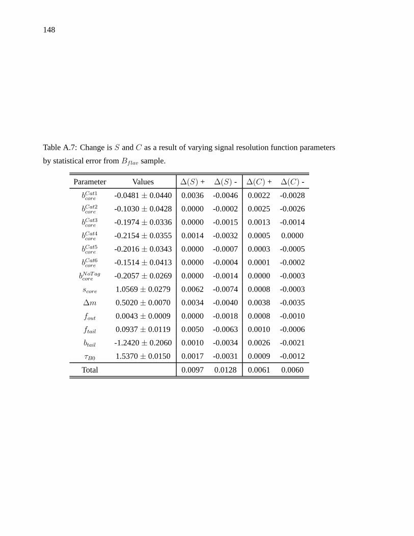
148

Table A.7: Change is S and C as a result of varying signal resolution function parameters

by statistical error from Bflav sample.


bCat1core -0.0481 ± 0.0440 0.0036 -0.0046 0.0022 -0.0028

bCat2core -0.1030 ± 0.0428 0.0000 -0.0002 0.0025 -0.0026

bCat3core -0.1974 ± 0.0336 0.0000 -0.0015 0.0013 -0.0014

bCat4core -0.2154 ± 0.0355 0.0014 -0.0032 0.0005 0.0000

bCat5core -0.2016 ± 0.0343 0.0000 -0.0007 0.0003 -0.0005

bCat6core -0.1514 ± 0.0413 0.0000 -0.0004 0.0001 -0.0002

bNoTagcore -0.2057 ± 0.0269 0.0000 -0.0014 0.0000 -0.0003

score 1.0569 ± 0.0279 0.0062 -0.0074 0.0008 -0.0003

∆m 0.5020 ± 0.0070 0.0034 -0.0040 0.0038 -0.0035

fout 0.0043 ± 0.0009 0.0000 -0.0018 0.0008 -0.0010

ftail 0.0937 ± 0.0119 0.0050 -0.0063 0.0010 -0.0006

btail -1.2420 ± 0.2060 0.0010 -0.0034 0.0026 -0.0021

τB0 1.5370 ± 0.0150 0.0017 -0.0031 0.0009 -0.0012

Total 0.0097 0.0128 0.0061 0.0060

References

[1] J.H. Christenson et al, Phys. Rev. Lett. 13, 138 (1964).

[2] A.D. Sakharov, Pisma Zh. Eksp. Theor. Fiz. 5, 32 (1967); JETP Lett. 5, 24 (1956).

[3] I. Bigi and A. Sanda, CP Violation, Cambridge University Press (2000).

[4] M. Kobayashi and T. Maskawa, Prog. Th. Phys. 49, 652 (1973).

[5] The BABAR Physics Book,edited by P. F. Harrison and H. R. Quinn,SLAC-R-504(1998).

[6] Heavy Flavor Averaging Group, Results on Time-DependentCP Measurements: Sum-mer 2005 (Lepton-Photon, Uppsala, Sweden and HEP 2005, Lisboa, Portugal) ,http://www.slac.stanford.edu/xorg/hfag/triangle/summer2005/, (2005).

[7] M. Gavela et al. Mod. Phys. Lett. A9, 895 (1994) and Nucl. Phys. B340, 382 (1994);P. Huet and E. Sather. Phys. Rev. D D51, 379 (1995).

[8] C.S. Wu, E. Ambler, R.Hayward, D. Hoppes, adn R. Hudson, Phys. Rev.105, 1413(1957).

[9] M. Goldhaber, L. Grodzinns, and A. Sunyar, Phys. Rev.109, 1015 (1958).

[10] F. Halzen and A. Martin, Quarks and Lepton: An Introductory Course in ModernParticle Physics, (1984).

[11] M.E. Peskin and D.V. Shroeder, An Introduction to Quantum Field Theory, (1995).

[12] G. Branco, L. Lavoura, J. Silva, CP Violation, Oxford University Press (1999).

[13] Particle Data Group, S. Eidelman et. al., Phys. Lett. B 592, 1 (2004).

[14] L. Wolfenstein, Phys. Rev. Lett. 51, 1945 (1983).

[15] Okubo, S. Phys. Lett., 1963, B5, 165. Zweig, G. CERN Report No.8419/TH412(1964). Iizuka, I. Prog. Theor., Phys. Suppl. 37, 1966, 38, 21.

[16] Y. Grossman and M. P. Worah, Phys. Lett. B 395, 241 (1997);

149

150

[17] M. Ciuchini, E. Franco, G. Martinelli, A. Masiero and L. Silvestrini, Phys. Rev. Lett.79, 978 (1997).

[18] T. Gershon and M. Hazumi, Phys. Lett. B 596, 163 (2004).

[19] H. Cheng, C. Chua, and A. Soni, hep-ph/0506268 (2005).

[20] G. Englehard, Y. Nir, and G. Raz, he-ph/0505194 (2005).

[21] BABAR Collaboration, B. Aubert et al, Nucl. Instr. Methods A479, 1 (2002).

[22] BABAR Collaboration, B. Aubert et. al., hep-ex/0408065 (2004).

[23] W. Verkerke and D. Kirkby, The RooFit Toolkit for Data Modelling,http://roofit.sourceforge.net/ (2005); R. Brun and F. Rademakers, Root: AnObject-Oriented Data Analysis Framework, http://root.cern.ch/ (2004).

[24] J. Smith, A. Soffer, and R. Waldi, Recommendation for Exclusive B ReconstructionAnalysis Variables, BABAR Note 497 (1999).

[25] J. Ocariz, M. Pivk, L Roos, A. Hoecker, H. Lacker, F.R. Le Diberder, BackgroundFighting in Charmless Two-Body Analyses, BABAR Analysis Document 346 (2002).

[26] BABAR Collaboration, B. Aubert et al, Phys. Rev. Lett. 93, 131805 (2004). (2004).

[27] D. Lange, G. Sciolla, M.C. Simani, Y. Zheng, BtgTest and Tag04: Studies Towardsan Improved Tagging Algorithm, BABAR Analysis Document 730

[28] Crystal Ball Collaboration, D. Antreasyan et al, Crystal Ball Note 321 (1983).

[29] ARGUS Collaboration, H. Albrecht et al, Phys. Lett. B 185, 218 (1987); 241, 278(1990).

[30] W. Hulsbergen, H. Jawahery, D. Kovalskyi, and M. Pierini , Measurement of thebranching ratio and the time-dependent CP asymmetries for B0 → K0

Sπ0 decays

on run 1-4 data ,

[31] M. Pivk and F. LeDiberder, physics/0402083 (2004). BABAR Analysis Document 904(2004).

[32] BABAR Collaboration, SVT misalignment files for 14-series data,http://www.slac.stanford.edu/BFROOT/www/Detector/SVT/LocalAlignment/systematics-14/ (2004).

[33] O. Long, M. Baak, R.N. Cahn, and D. Kirkby, Phys. Rev. D 68, 034010 (2003).

[34] BABAR Collaboration, B. Aubert et al, Phys. Rev. Lett. 95, 011801 (2005).

[35] Belle Collaboration, K. Sumisawa et al, Phys. Rev. Lett. 95, 061801 (2005)

151

[36] Heavy Flavor Averaging Group, Results on Time-Dependent CP Measurements: Winter (Moriond) 2005.,http://www.slac.stanford.edu/xorg/hfag/triangle/moriond2005/index.shtml, (2005).

[37] K. Trabelsi, sin 2φ1 Charmless and Radiative Decays,http://www.lip.pt/events/2005/hep2005/talks/hep2005 talk KarimTrabelsi.pdf,(2005).

[38] M. Beneke, Phys. Lett. B 620 143 (2005).

[39] BABAR Collaboration, B. Aubert et. al., hep-ex/0507052 (2005).

the measurement of cp asymmetries in the three-body

Documents