the maxwell-stefan diffusion limit for a kinetic model of

HAL Id: hal-01303312https://hal.inria.fr/hal-01303312

Submitted on 17 Apr 2016

HAL is a multi-disciplinary open accessarchive for the deposit and dissemination of sci-entific research documents, whether they are pub-lished or not. The documents may come fromteaching and research institutions in France orabroad, or from public or private research centers.

L’archive ouverte pluridisciplinaire HAL, estdestinée au dépôt et à la diffusion de documentsscientifiques de niveau recherche, publiés ou non,émanant des établissements d’enseignement et derecherche français ou étrangers, des laboratoirespublics ou privés.

The Maxwell-Stefan diffusion limit for a kinetic model ofmixtures with general cross sections

Laurent Boudin, Bérénice Grec, Vincent Pavan

To cite this version:Laurent Boudin, Bérénice Grec, Vincent Pavan. The Maxwell-Stefan diffusion limit for a kineticmodel of mixtures with general cross sections. Nonlinear Analysis: Theory, Methods and Applications,Elsevier, 2017, 159, pp.40-61. �10.1016/j.na.2017.01.010�. �hal-01303312�

https://hal.inria.fr/hal-01303312

https://hal.archives-ouvertes.fr

THE MAXWELL-STEFAN DIFFUSION LIMIT FOR A KINETIC MODEL

OF MIXTURES WITH GENERAL CROSS SECTIONS

LAURENT BOUDIN, BÉRÉNICE GREC, AND VINCENT PAVAN

Abstract. In this article, we derive the Maxwell-Stefan formalism from the Boltzmann equation formixtures for general cross-sections. The derivation uses the Hilbert asymptotic method for systemsat low Knudsen and Mach numbers. We also formally prove that the Maxwell-Stefan coe�cientscan be linked to the direct linearized Boltzmann operator for mixtures. That allows to compute thevalues of the Maxwell-Stefan di�usion coe�cients with explicit and simple formulae with respectto the cross-sections. We also justify the speci�c ansatz we use thanks to the so-called momentmethod.

1. Introduction and motivations

The study of mass transport in a gaseous mixture is one of the oldest topics investigated inmechanics and thermodynamics. The earliest contributions about mass transport by di�usion canbe traced back to the nineteenth century: Graham [26], Fick [21], Maxwell [37], Stefan [44], toname a few, but probably the most celebrated ones. Later on, in 1968, Onsager's Nobel prizeconsecrated decisive works regarding thermodynamic aspects of such mass transport. An intrinsicdi�culty consists in understanding the various di�usion laws previously introduced. In particular,the eagerness to identify both liquid and gas di�usions as a molecular mechanism can be interpretedas a mean to prove the existence of atoms as constitutive elements of matter. From this point ofview, Perrin obtained his Nobel prize in 1926 for his early works [40] about the Brownian motion,hence clearly focused on di�usion, but awarded as a decisive contribution to the proof of matterdiscontinuity, linked to the discussion about atoms.

Di�usion is always a motion of a chemical species through something else, which can be either otherchemical species, surrounding solvent particles, or solid systems. Consequently, di�usion phenomenafor liquids and solids often distinguish from the gaseous ones. In the �rst case, the species of interestis not the dominant element: the solvent (water, for instance) or the solid matrix (crystallographicbody) is the main matter inside which the transport takes place. As a consequence, in a liquidor a solid, there is in general no notion of spatial inhomogeneity (and hence no gradient of matterquantity) of the surrounding background. Hence, any phenomenological law for transport only takesinto account the gradient of the transported species itself. This situation, which is speci�c to liquidsor solids, is very di�erent in the case of gaseous di�usion.

Since it models some kind of motion, gaseous di�usion needs to be linked to forces. This is nota simple problem, resulting from Newton's law for motion. Indeed, the di�culty mainly lies in thefacts that it is sometimes di�cult to de�ne the systems of which the movement must be explained,and that the forces they undergo take place at the molecular level, where the deterministic viewpointmust be replaced by random and statistical considerations.

Among the most ancient problems regarding mass transport in mixtures lies the surprising debatebetween Fick and Maxwell-Stefan's laws tenants. Plenty of literature has been written on the topic,and we do not pretend to provide any kind of review regarding it in this article. The presentations ofthese laws are either essentially phenomenological (Maxwell-Stefan) or theoretically axiomatic (Fick,with Onsager's contributions). Let us just mention one example of the controversy: Duncan and

Date: April 17, 2016.This work was partially funded by the French ANR-13-BS01-0004 project Kibord headed by L. Desvillettes.

1

2 L. BOUDIN, B. GREC, AND V. PAVAN

Toor [20] investigate three-species gaseous mixtures, and point out the possibility of transport of aspecies when it has no initial gradient (of quantity of matter) as an original phenomenon, whereasit is quite clear that the Onsager theory allows it.

The striking formal analogy between Fick and Maxwell-Stefan formulations incites some authorsto state that both approaches are the same one. They propose numerical methods to link thephysical coe�cients in both formulations, see for instance [23, 3]. But such a uni�cation remainsquite unclear: the physical reasons invoked to derive the regimes do not really match. Indeed,Fick deals with mass conservations and Maxwell-Stefan with momentum equations. Moreover, itis restricted to the computation of the Maxwell-Stefan coe�cients from the Fick ones and not theconverse, since, so far, up to our knowledge, no computation of the Maxwell-Stefan coe�cients wereavailable from the Boltzmann equation.

Our point of view is quite simple and constructive altogether: as far as dilute gases are concerned,any macroscopic transport phenomenon should be somehow derived from the Boltzmann equation formixtures. Indeed, the Boltzmann equation can really take into account molecular interactions whichqualitatively explain many di�usion processes. Roughly speaking, it has been proved, sometimesrigorously, for mono-species systems, that the Boltzmann equation allows to recover continuoustransport processes in gases, and moreover to compute the involved physical coe�cients, see [1,2, 25, 38]. Continuing the work initiated in [7], we here show how it is possible to recover theMaxwell-Stefan formalism from the Boltzmann equation, as it is commonly known for Fick's law.A cornerstone of this work is the di�erence between the Chapman-Enskog development and theso-called rational extended thermodynamics, also known as the moment method. The �rst one leadsto the Onsager/Fick formalism, and the second one to the Maxwell-Stefan theory.

The reason why one method should be preferentially used to the other also remains controver-sial. A key argument was given by Levermore [34] when explaining his moment closure hierarchymethodology:

�More precisely, we seek models that properly capture the �uid dynamical regimewhen the mean free path is much smaller than the macroscopic length scales, whilein the transition regime they give values for the momentum and energy �uxes (andother quantities) that are at least consistent with the nonnegativity of the particledensity, and are thereby hopeful of the correct order of magnitude. By doing so, suchmodels may provide a bridge over the transition regime that may be useful in theconstruction of hybrid �uid/kinetic simulations.�

To state it by other means, the moment method, which, in our case, is also derived from the Hilbertexpansion method, can be seen as a systematic way to reach gas dynamics which is neither at localequilibrium (Euler equations), nor very close to it (hydrodynamical regime which, in the mixturecase, covers Fick's formalism). Such an assumption has received an important numerical agreement,as stated in [31, 32]: the moment method apparently produces equations which seem to �t anincreasing rarefaction, whereas the Chapman-Enskog expansion and its continuations (Burnett) donot.

Let us discuss some more details about both di�usion theories. We must emphasize that bothequations lie in the cross di�usion models, which �rst arose in population dynamics [43, 36, 35] andare currently widely studied from the mathematical viewpoint, see [14, 33, 18, 28] and the referencestherein. We deal with an ideal gas mixture constituted with I ≥ 2 species (Ai). For each i, 1 ≤ i ≤ I,we introduce ni the number of molecules of Ai, depending on time t ∈ R+ and position x ∈ R3. Wealso de�ne the associated �ux Ni of species Ai. Let ν =

∑ni be the total number of molecules in

the mixture and set ξi = ni/ν the mole fraction of species Ai.

MAXWELL-STEFAN LIMIT FOR A KINETIC MODEL WITH GENERAL CROSS SECTIONS 3

The Maxwell-Stefan equations give relationships between the �uxes and the mole fractions. Theyare written

(1) −ν∇xξi =∑j 6=i

ξjNi − ξiNj

Ð ij, 1 ≤ i ≤ I

where Ð ij > 0 is the e�ective di�usion coe�cient between species Ai and Aj . For physical reasons,the di�usion coe�cients are symmetric with respect to the particles exchange, i.e. Ð ij = Ð ji.Note that there are exactly (I − 1) independent equalities of type (1). The origin of (1) reliesforce considerations and stems from momentum equations. In fact, (1) translates, for species Ai,the balance between the friction forces and the pressure ones. The main assumption of this model,which surely does not go by itself, is the fact that the di�erent species have di�erent macroscopic

velocities on macroscopic time scales.The thermodynamics of irreversible processes viewpoint is apparently very di�erent from the

Maxwell-Stefan description. It claims that the main reason for change in particle systems is notmacroscopic mechanics (second Newton's law) but rather thermodynamics (principle of entropyminimization). Following this approach, a few quantities of interest (mass, momentum, energy, etc.)are transferred in systems because of the entropy organization. The main notion is then the oneof �ux, which usually di�ers from the notion of macroscopic mechanical movement). It enables thedescription of the spatial transfer rate. Close to equilibrium, linear considerations are invoked tomodel the �uxes as linear combinations of the so-called �generalized driving forces� (which actually donot have the physical dimension of a force). In general [24], �uxes are written as linear combinationsof potential symmetrical gradient following

Ni =I∑j=1

Λij : ∇sxΠj ,

where the symmetrical tensors Ni denote the �uxes and the symmetrized tensors ∇sxΠj are thepotentials. The linear coe�cients Λij are, in fact, tensors, while the symbol : denotes the generaltensor contraction product. The choice of �uxes and potentials is crucial, as well as the propertiesof the matrices Λij . In non reactive mixtures, under isothermal conditions, the �ux Ni of moleculesof species Ai is usually written as

Ni =

I∑j=1

λij∇x(µjT

),

where µj are chemical potentials, and the λij are the Onsager scalar coe�cients. For ideal gases,under isothermal conditions (constant temperature T ), the term ∇x

(µjT

)reduces to ∇xnj/nj , and

it comes

Ni = −I∑j=1

Dij∇xnj ,

where Dij are the Fick coe�cients. In order to enforce entropy decay, which is the main approachof the system, the Onsager scalar matrix λij needs to be symmetrical and non positive. Finally, ifwe assume that the total number of molecules in the system, which is ν =

∑ni, does not depend

on space and time, we can write (see also [16])

(2) Ni = −νI∑j=1

Dij∇xξj ,

with Dij = λij/nj > 0.Equations (1) and (2) look very similar, at least in the choice of the unknown functions. More

precisely, in the Maxwell-Stefan system (1), the quantities ∇xξi are written as explicit linear com-binations of the �uxes Nj , while in Fick's law (2), the �uxes Ni are explicit linear combinations


of the ∇xξj . This analogy between Maxwell-Stefan and Fick formulations has conducted people topostulate a relation between the coe�cients. The main reason to unify both formulations lies on mi-croscopic considerations about colliding molecules. If we trust any of the above equations, they needto describe the same phenomena at the microscopic level. However, though formulations (1) and (2)are matricially inverse to each other, inversion does not go by itself [24, 3], and the question of thephysical justi�cation is often eluded. This can be explained by the fact that axiomatic macroscopicdi�usion theories cannot provide enough information on the di�usion coe�cients to deduce somerelevant mathematical properties on the involved matrices of coe�cients. Moreover, whereas Fickand Maxwell-Stefan's processes naturally originate from micro-collisions between molecules, theydo not belong to the same regime. Note that [13, 4] provides a discussion about possible di�usionmodels in the lung, and that the Maxwell-Stefan equations were mathematically studied in [3, 6, 29],and eventually coupled with the Navier-Stokes equations [15], whereas Fick's law was investigatedfor instance in [24, 3] and many references therein.

In this article, we show how it is possible to derive the Maxwell-Stefan formalism from the Boltz-mann equation modelling particles mixtures. The kinetic model, presented in various forms in[22, 19, 12, 7] and mathematically investigated in [5, 17, 11, 10], is �rst described in Section 2. Thederivation is then performed in Section 3, by using the Hilbert asymptotic method for systems atlow Knudsen and Mach numbers. We also formally prove that the Maxwell-Stefan coe�cients canbe straightforwardly linked to the direct linearized Boltzmann operator for mixtures. That allowsus to provide the values of the Maxwell-Stefan coe�cients with explicit and simple formulae withrespect to the cross-sections. For the model derivation, we use a speci�c ansatz which we justify inAppendix A thanks to the moment method [34].

The present work is the natural continuation of [7], but with the notable fact that it completes thee�ciency of the method to any kind of molecules interactions (with Grad's cuto� assumption) andnot only Maxwellian molecules. Let us also mention the work in [27], where the authors choose aparticular form of analytic cross sections, and perform explicit computations of the Maxwell-Stefandi�usion coe�cients.

2. Kinetic model for monatomic gaseous mixtures

We �rst introduce the kinetic setting for monatomic gaseous mixtures. For each species Ai ofmolecular mass mi, the unknown function is the number density function fi. This function dependson space coordinates x ∈ R3 (or any subdomain of interest), time t ≥ 0, and velocity v ∈ R3. Moreprecisely, fi(t, x, v) dx dv is the number of molecules of species Ai in the mixture, at time t in anelementary volume of the space phase of size dx dv centred at (x, v). The number density functionssatisfy the Boltzmann equations, which read as follows, for any i ∈ J1, IK,

(3) ∂tfi + v · ∇xfi =

I∑j=1

Qij(fi, fj) on R3 × R∗+ × R3,

where the notation J1, IK denotes [1, I]∩N. These equations can also be written in a vector sense as

∂tf + v · ∇xf = Q(f, f) on R3 × R∗+ × R3,

where f = (f1, · · · , fI)ᵀ and

Q(f, f) =

I∑j=1

Q1j(f1, fj), · · · ,I∑j=1

QIj(fI , fj)

ᵀ .To specify the operator Q(f, f), we �rst need to describe the collision mechanism between two

molecules of species Ai and Aj , 1 ≤ i, j ≤ I, with respective pre-collisional velocities v′, v′∗. After


a collision, their velocities are denoted by v and v∗. Since the collisions are supposed to be elastic,both momentum and kinetic energy are conserved, i.e.

(4) miv′ +mjv

′∗ = miv +mjv∗,

1

2mi |v′|2 +

1

2mj |v′∗|2 =

1

2mi |v|2 +

1

2mj |v∗|2.

It is then standard, from (4), to write v′ and v′∗ as

(5) v′ =1

mi +mj(miv +mjv∗ +mj |v − v∗|σ), v′∗ =

1

mi +mj(miv +mjv∗ −mi|v − v∗|σ),

where σ ∈ S2 is a parameter taking into account both degrees of freedom allowed by (4). Denoting

πij(v, v∗, σ) := v′ =1

mi +mj(miv +mjv∗ +mj |v − v∗|σ),

it is straightforward to check that, for any vector w ∈ R3 and rotation Θ ∈ O+(R3),

(6) πij(v + w, v∗ + w, σ) = πij(v, v∗, σ) + w, πij(Θv,Θv∗,Θσ) = Θπij(v, v∗, σ), ∀v, v∗, σ,

where O+(R3) denotes the three-dimensional rotation group. This observation will be useful in thesequel.

The microscopic equalities (5) are used in the expressions of the collision operators Qij , describingthe interactions between molecules of species Ai and Aj , 1 ≤ i, j ≤ I. For any functions f ,g : R3 → R+, we de�ne the following operator

(7) Qij(f, g)(v) =

∫R3

∫S2Bij(v, v∗, σ)

[f(v′)g(v′∗)− f(v)g(v∗)

]dσ dv∗,

where v′ and v′∗, are de�ned through (5), and the cross section Bij satis�es the microreversibilityassumptions Bij(v, v∗, σ) = Bji(v∗, v, σ) and Bij(v, v∗, σ) = Bij(v

′, v′∗, σ).It is worthwhile noting that the operator describing the collisions of molecules of species Aj

with molecules of species Ai is not de�ned using (5), but involving the symmetrical pre-collisionalvelocities w′ and w′∗ given by

w′ =1

mi +mj(mjv +miv∗ +mi|v − v∗|σ), w′∗ =

1

mi +mj(mjv +miv∗ −mj |v − v∗|σ).

Consequently, we have

Qji(g, f)(v) =

∫R3

∫S2Bji(v, v∗, σ)

[g(w′)f(w′∗)− g(v)f(v∗)

]dσ dv∗.

Let us emphasize that the main di�erence of this work with [7] lies in the fact that we deal withgeneral cross-sections with angular cut-o�, instead of the simpler case of Maxwell molecules. Thecross sections are only assumed to satisfy the standard Galilean invariance properties: for any i, j,vector w ∈ R3, and rotation Θ ∈ O+(R3), we have

(8) Bij(v + w, v∗ + w, σ) = Bij(v, v∗, σ), Bij(Θv,Θv∗,Θσ) = Bij(v, v∗, σ), ∀v, v∗, σ.Further notations are useful to write standard weak formulations of the collision operators. We

set, for any g, h ∈ L2(R3),

(9) 〈g, h〉 =

∫R3

g(v)h(v) dv,

and, for any g, h ∈ L2(R3)I ,

(10) 〈g, h〉I =

I∑i=1

〈gi, hi〉.


Note that both previous notations can also be de�ned if h or its components take their values inthe velocity space R3. They can also be extended, in a duality sense, whenever the products gh in(9) or gihi in (10) are in L1(R3). That allows to write, for any relevant test-function ψ, scalar orvector-valued,

〈Qij(f, g), ψ〉 =

∫∫∫Bij f(v) g(v∗)

[ψ(v′)− ψ(v)

]dσ dv∗ dv,(11)

〈Qij(f, g), ψ〉 = −1

2

∫∫∫Bij

[f(v′) g(v′∗)− f(v) g(v∗)

] [ψ(v′)− ψ(v)

]dσ dv∗ dv.(12)

In particular, (11)�(12) imply that, for any i and j,∫R3

Qij(f, g)(v) dv = 0,(13) ∫R3

Qij(f, g)(v)mi v dv +

∫R3

Qji(g, f)(v)mj v dv = 0,(14) ∫R3

Qij(f, g)(v)1

2mi |v|2 dv +

∫R3

Qji(g, f)(v)1

2mj |v|2 dv = 0.(15)

Note that, if i = j, (14)�(15) reduce to the classical equalities for the Boltzmann collision operator,which are

(16)

∫R3

Qii(f, g)(v) v dv = 0,

∫R3

Qii(f, g)(v)1

2|v|2 dv = 0.

More details about the monatomic mixture model, including the weak forms of the collisionoperators, can be found, for instance, in [7].

Before introducing the associated macroscopic equations, we set, whenever it makes sense, for anyreal-valued function f ,

f =

∫R3

f(v) dv,

and, for any vector-valued function f = (f1, · · · , fI),

f =I∑i=1

fi.

We de�ne, for any i, the following macroscopic quantities as moments of the distribution functionfi, i.e.

ni = fi =

∫R3

fi(v) dv, niui = vfi =

∫R3

vfi(v) dv,

where ni is the number of molecules of species Ai, and ui is its associated macroscopic velocity.Then we denote by ρi = mini the total mass of molecules of species Ai, and de�ne the total energyof the mixture

E =1

2

I∑i=1

miv2fi =1

2

I∑i=1

∫R3

miv2fi(v) dv.

From these quantities, we introduce the total number of molecules ν =∑ni, the total mass of the

mixture ρ =∑ρi, the molar bulk velocity u =

∑niui/ν, and eventually the mixture temperature

T thanks to the formula E = 1/2ρu2 + 3/2νkBT .

We can choose to write fi as a local Maxwellian in the velocity variable, i.e. with the form(17)

fi(t, x, v) = ni(t, x)

(mi

2πkBT (t, x)

)3/2

exp

(−mi|v − ui(t, x)|2

2kBT (t, x)

), x ∈ R3, t > 0, v ∈ R3.


This corresponds to assuming small values of the Knudsen number. If we force the Boltzmannequations (3) with this family of functions, then, after integration over the kinetic functions forindividual mass, individual velocity and total energy, it is straightforward to check that, for any i,

∂tni +∇x · (niui) = 0,(18)

∂t(ρiui) +∇x · (ρiui ⊗ ui) +∇x (kBTni) =∑j 6=i

∫R3

miv Qij(fi, fj)(v) dv,(19)

∂tE +∇x · ((E + νkBT )u) = 0,(20)

where the term with j = i vanishes in the right-hand side of (19) thanks to the conservation prop-erties of the mono-species collision operators (16). The choice of Ansatz (17) and the computationof the above moment equations (18)�(20) are discussed in Section A and in Appendix A.2. Theremaining question is the computation of the right-hand side term of (19), which is performed inthe next section, in the limit of vanishing Mach numbers.

3. Computations of the Maxwell-Stefan diffusion coefficients

Let us now study the di�usion asymptotics of the Boltzmann equations for mixtures, which willallow to obtain expressions of the Maxwell-Stefan di�usion coe�cients with respect to general cross-sections (Bij) while recovering the symmetry feature and the nonnegativity of the (Ð ij).

3.1. Scaling the Boltzmann equations. We use the mean free path ε > 0 as the asymptoticparameter to reach the classical di�usion limit (i.e. we perform the classical di�usive scaling in theBoltzmann equation x = x/ε, t = t/ε2). In this setting, we also assume that both Knudsen andMach numbers are of order ε.

If we denote f ε = (f ε1 , · · · , fεI ) the unknown function (the ∼ notations for x and t are thendropped), we can write

(21) ε ∂tfεi + v · ∇xf εi =

1

ε

I∑j=1

Qij(fεi , f

εj ), on R3 × R∗+ × R3, 1 ≤ i ≤ I.

The penalisation by 1/ε on the right-hand side term of (21) implies that f ε is close to the globalequilibrium. Following Ansatz (17), if we moreover consider small values of the Mach number, wecan assume that(22)

f εi (t, x, v) = nεi (t, x)

(mi

2πkB T ε(t, x)

)3/2

e−mi|v−εuεi (t,x)|2/2kBT ε(t,x), x ∈ R3, t > 0, v ∈ R3,

with nεi : R3 × R+ → R+, uεi : R3 × R+ → R3, for 1 ≤ i ≤ I, and T ε : R3 × R+ → R∗+. All

macroscopic quantities de�ned above are of order 0 in ε. Consequently, functions satisfying (22) areclose to the global equilibrium. It is the same framework as in [7].

In the same way as we got the moment equations (18)�(20) from Ansatz (17), we can obtainthe following system from the scaled Ansatz (22). Note that, obviously, those moment equationscan also be built from (18)�(20) with the classical di�usive scaling. Hence, in the same way as wede�ned f ε from f , we add the dependence with respect to ε on all the notations de�ned at the endof Section 2 for the macroscopic quantities. Consequently, that allows us to write, for any i,

ε∂tnεi + ε∇x(nεiu

εi ) = 0,

ε2∂t(ρεinεiuεi ) +∇x · (ε2ρεiuεi ⊗ uεi ) +∇x(kBT

εnεi ) =1

ε

∑j 6=i〈Qij(f εi , fεj ),miv〉,

ε∂t(ε2ρεuε2 + 3kBT

ενε) + ε∇x · [(ε2ρε(uε)2 + 5kBTενε)uε] = 0.


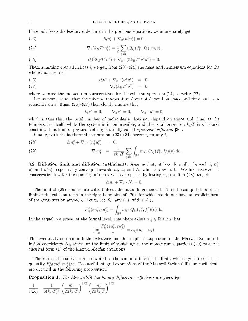
If we only keep the leading order in ε in the previous equations, we immediately get

∂tnεi +∇x(nεiu

εi ) = 0,(23)

∇x(kBTεnεi ) =

1

ε

∑j 6=i〈Qij(f εi , fεj ),miv〉,(24)

∂t(3kBTενε) +∇x · (5kBT ενεuε) = 0.(25)

Then, summing over all indices i, we get, from (23)�(24) the mass and momentum equations for thewhole mixture, i.e.

∂tνε +∇x · (νεuε) = 0,(26)

∇x(kBTενε) = 0,(27)

where we used the momentum conservations for the collision operators (14) to write (27).Let us now assume that the mixture temperature does not depend on space and time, and con-

sequently on ε. Eqns. (25)�(27) then clearly implies that

∂tνε = 0, ∇xνε = 0, ∇x · uε = 0,

which means that the total number of molecules ν does not depend on space and time, as thetemperature itself, while the system is incompressible, and the total pressure νkBT is of courseconstant. This kind of physical setting is usually called equimolar di�usion [30].

Finally, with the isothermal assumption, (23)�(24) become, for any i,

∂tnεi +∇x · (nεiuεi ) = 0,(28)

∇xnεi =1

εkBT

∑j 6=i

∫R3

miv Qij(fεi , f

εj )(v) dv.(29)

3.2. Di�usion limit and di�usion coe�cients. Assume that, at least formally, for each i, nεi ,uεi and nεiu

εi respectively converge towards ni, ui and Ni when ε goes to 0. We �rst recover the

conservation law for the quantity of matter of each species by letting ε go to 0 in (28), to get

∂tni +∇x ·Ni = 0.

The limit of (29) is more intricate. Indeed, the main di�erence with [7] is the computation of thelimit of the collision term in the right hand side of (29), for which we do not have an explicit formof the cross section anymore. Let us set, for any i, j, with i 6= j,

F εij(εuεi , εu

εj) =

∫R3

miv Qij(fεi , f

εj )(v) dv.

In the sequel, we prove, at the formal level, that there exists αij ∈ R such that

limε→0

F εij(εuεi , εu

εj)

ε= αij(ui − uj).

This eventually ensures both the existence and the �explicit� expression of the Maxwell-Stefan dif-fusion coe�cients Ð ij since, at the limit of vanishing ε, the momentum equations (29) take theclassical form (1) of the Maxwell-Stefan equations.

The rest of this subsection is devoted to the computations of the limit, when ε goes to 0, of thequantity F εij(εu

εi , εu

εj)/ε. Two useful integral expressions of the Maxwell-Stefan di�usion coe�cients

are detailed in the following proposition.

Proposition 1. The Maxwell-Stefan binary di�usion coe�cients are given by

1

νÐij=

1

6(kBT )2

(mi

2πkBT

)3/2( mj

2πkBT

)3/2

MAXWELL-STEFAN LIMIT FOR A KINETIC MODEL WITH GENERAL CROSS SECTIONS 9∫∫∫Bij(v, v∗, σ) exp

[− mi

2kBTv2 − mj

2kBTv∗

2

][mi(v

′ − v)]2 dσ dv∗ dv(30)

=mimj

6(kBT )2(mi +mj)

(mi

2πkBT

)3/2( mj

2πkBT

)3/2

∫∫∫Bij(v, v∗, σ) exp

[− mi

2kBTv2 − mj

2kBTv∗

2

](v − v∗ + |v − v∗|σ) · (miv −mjv∗) dσ dv∗ dv.(31)

We must emphasize that (30) ensures the nonnegativity of the coe�cients, while (31) allows tocheck their symmetry property.

Let us now focus on the formal proof of Proposition 1, with the study of F εij(εuεi , εu

εj)/ε. Using

Ansatz (22) and (11) with ψ(v) = miv, we can write

F εij(εuεi , εu

εj) =

(mi

2πkBT

)3/2( mj

2πkBT

)3/2

nεinεj∫∫

R6

∫S2Bij(v, v∗, σ) exp

[− mi

2kBT(v − εuεi )2

]exp

[− mj

2kBT(v∗ − εuεj)2

]mi(v

′ − v) dσ dv∗ dv.

Let us �rst state some properties of F εij when ε is �xed, which are direct consequences of the

Galilean invariance properties (8) of Bij , and the properties (6) of v′.

Lemma 1. For any u1, u2, w ∈ R3 and Θ ∈ O+(R3),

(32) F εij(εu1 + w, εu2 + w) = F εij(εu1, εu2), F εij(εΘu1, εΘu2) = ΘF εij(εu1, εu2).

Proof. This is proven by changing variables. In the �rst equation, we set V = v − w, V∗ = v∗ − w,then write∫

Bij(v, v∗, σ) exp

[− mi

2kBT(v − εu1 − w)2 − mj

2kBT(v∗ − εu2 − w)2)

]mi (πij(v, v∗, σ)− v) dv dv∗ dσ

=

∫Bij(V + w, V∗ + w, σ) exp

[− mi

2kBT(V − εu1)2 −

mj

2kBT(V∗ − εu2)2

]mi (πij(V + w, V∗ + w, σ)− V − w) dV dV∗ dσ,

and eventually use (6) and (8). In the second one, we write ΘV = v, ΘV∗ = v∗, ΘΣ = σ, thenobtain∫

Bij(v, v∗, σ) exp

[− mi

2kBT(v − εΘu1)2 −

mj

2kBT(v∗ − εΘu2)2

]mi (πij(v, v∗, σ)− v) dV dV∗ dσ

=

∫Bij(ΘV,ΘV∗,ΘΣ) exp

[− mi

2kBT(ΘV − εΘu1)2 −

mj

2kBT(ΘV∗ − εΘu2)2

]mi (πij(ΘV,ΘV∗,ΘΣ)−ΘV ) dV dV∗ dΣ,

use (6) and (8) again, and the fact that Θ is an isometry. Note that, in both cases, the Jacobian ofthe changes of variables is 1. �

Let us now deal with the asymptotic behaviour of F εij(εuεi , εu

εj)/ε when ε goes to 0. Because of

(32), we deduce that

F εij(εuεi , εu

εj) = F εij(εu

εi − εuεj , 0) = F εij(0, εu

εj − εuεi ).


We are thus led to investigate the asymptotic behaviour of

Hεij(u

εij) =

1

2ε

(F εij(εu

εij , 0) + F εij(0,−εuεij)

)=

1

εF εij(εu

εij , 0) =

1

εF εij(0,−εuεij),

where we set uεij = uεi − uεj . Note that the previous equality also allows to de�ne Hεij as an operator

acting on any vector of R3.Let ni, nj , ui and uj denote the respective formal limits of (nεi ), (nεj), (uεi ) and (uεj) when ε goes

to 0. More precisely, we assume that each quantity depending on ε di�ers from its limit by O(ε).

Lemma 2. The following equality holds at the formal level:

(33) Hεij(u

εij) = − mi

2

2kBT

(mi

2πkBT

)3/2( mj

2πkBT

)3/2

ninj[∫∫∫Bij(v, v∗, σ) exp

[− mi

2kBTv2 − mj

2kBTv∗

2

][(v′ − v)]⊗2 dσ dv∗ dv

](ui − uj) +O(ε).

Proof. Using weak form (12), we can write, for any u ∈ R3,

(34) Hεij(u) = −1

ε

(mi

2πkBT

)3/2( mj

2πkBT

)3/2

nεinεj

∫∫∫Bij(v, v∗, σ)(

exp

[− mi

2kBT(v′ − εu)2

]exp

[− mj

2kBTv′∗

2]− exp

[− mi

2kBT(v − εu)2

]exp

[− mj

2kBTv∗

2

])mi(v


We �rst use the fact that

exp

[− mi

2kBTv′

2]

exp

[− mj

2kBTv′∗

2]

= exp

[− mi

2kBTv2]

exp

[− mj

2kBTv∗

2

],

then use the following expansions with respect to ε:

exp

[− mi

2kBTε2u2

]= 1 +O(ε2), exp

[mi

kBTεv′ · u

]= 1 + ε

mi

kBTv′ · u+ v′

2O(ε2),

as well as the similar ones for the other exponential term. Taking u = uεij in (34) implies, aftersimpli�cation by ε,

Hεij(u

εij) = −

(mi

2πkBT

)3/2( mj

2πkBT

)3/2

(ni +O(ε))(nj +O(ε))∫∫∫Bij(v, v∗, σ) exp

[− mi

2kBTv2]

exp

[− mj

2kBTv∗

2

][mi

kBT(v′ − v) · (ui − uj) +

(1 + |v′|+ |v|+ v′

2+ v2

)O(ε)

]mi(v


The term in O(ε) in the previous integral remains integrable in both variables v and v∗, thanks tothe collision rule (5) and the exponential functions, so that we eventually get (33). �

Remark 1. As we shall see in the next subsection, Proposition 2 is in fact directly linked to the

nonnegativity of the linearized Boltzmann operator for mixtures, see also [17].

Lemma 3. The following equality holds at the formal level:

(35) Hεij(u

εij) =

mi

2kBT

(mi

2πkBT

)3/2( mj

2πkBT

)3/2

ninj

MAXWELL-STEFAN LIMIT FOR A KINETIC MODEL WITH GENERAL CROSS SECTIONS 11[∫∫∫Bij(v, v∗, σ) exp

[− mi

2kBTv2 − mj

2kBTv∗

2

](v∗ − v + |v − v∗|σ)⊗ (miv −mjv∗) dσ dv∗ dv

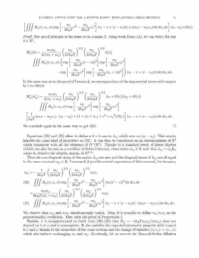
](ui−uj)+O(ε).

Proof. The proof principle is the same as in Lemma 2. Using weak form (11), we can write, for anyu ∈ R3,

Hεij(u) =

mimj

2ε(mi +mj)

(mi

2πkBT

)3/2( mj

2πkBT

)3/2

nεinεj∫∫∫

Bij(v, v∗, σ)

(exp

[− mi

2kBT(v − εu)2

]exp

[− mj

2kBTv∗

2

]− exp

[− mi

2kBTv2]

exp

[− mj

2kBT(v∗ + εu)2

])(v∗ − v + |v − v∗|σ) dσ dv∗ dv.

In the same way as in the proof of Lemma 2, we use expansions of the exponential terms with respectto ε to obtain

Hεij(u

εij) =

mimj

2(mi +mj)

(mi

2πkBT

)3/2( mj

2πkBT

)3/2

(ni +O(ε))(nj +O(ε))∫∫∫Bij(v, v∗, σ) exp

[− mi

2kBTv2]

exp

[− mj

2kBTv∗

2

][

1

kBT(miv −mjv∗) · (ui − uj) +

(1 + |v|+ |v∗|+ v2 + v∗

2)O(ε)

](v∗ − v + |v − v∗|σ) dσ dv∗ dv.

We conclude again in the same way to get (35). �

Equations (33) and (35) allow to de�ne a 3× 3 matrix Lij which acts on (ui − uj). This matrixinherits the same kind of properties as (32). It can thus be considered as an endomorphism of R3

which commutes with all the elements of O+(R3). Thanks to a standard result of linear algebra(which can also be seen as a corollary of Schur's lemma), there exists αij ∈ R such that Lij = αijI3,where I3 denotes the identity matrix of R3×3.

Thus the non-diagonal terms of the matrix Lij are zero and the diagonal terms of Lij are all equalto the same constant αij ∈ R. Lemmas 2�3 provide several expressions of this constant, for instance,

αij =− 1

6kBT

(mi

2πkBT

)3/2( mj

2πkBT

)3/2

ninj∫∫∫Bij(v, v∗, σ) exp

[− mi

2kBTv2 − mj

2kBTv∗

2

][mi(v

′ − v)]2 dσ dv∗ dv(36)

=mimj

6kBT (mi +mj)

(mi

2πkBT

)3/2( mj

2πkBT

)3/2

ninj∫∫∫Bij(v, v∗, σ) exp

[− mi

2kBTv2 − mj

2kBTv∗

2

](v∗ − v + |v − v∗|σ) · (miv −mjv∗) dσ dv∗ dv.(37)

We observe that αij and ninj simultaneously vanish. Thus, it is possible to de�ne αij/ninj as theproportionality coe�cient. That ends the proof of Proposition 1.

Besides, it is straightforward to check from (36)�(37) that Ð ij = −(kBTninj)/(ναij) does notdepend on t or x and is nonnegative. It also satis�es the expected symmetry property with respectto i and j, thanks to the properties of the cross sections and the change of variables (v, v∗) 7→ (v∗, v),which also induces exchanging mi and mj . Eventually, let us recover the Maxwell-Stefan di�usion


equations by letting ε go to 0 in (29). We immediately get, for any i,

∇xni =1

ν

∑j 6=i

ninj(ui − uj)Ð ij

,

which yields (1).

Remark 2. Noticing that the right-hand side of (29) converges, when ε vanishes, to

1

kBT

∑j 6=i

αij(ui − uj),

it is quite natural to set, for any i,

(38) αii = −∑j 6=i

αij ,

so that the limit term in the right-hand side of (29) reads

− 1

kBT

I∑j=1

αijuj .

That allows to de�ne the matrix A = (αij)1≤i,j≤I ∈ RI×I , which depends on (ni), and write the

asymptotics of (29), for any i, under the usual matrix form [24]

∇xni = − 1

kBT[AU ]i,

where U denotes the column vector (u1, · · · , uI)ᵀ.It is then clear that A is symmetric, negative semi-de�nite, and rankA = I − 1. The symmetry

is straightforwardly obtained from (37). Moreover, we can compute, for any U ∈ RI ,

AU · U =∑i,j

αijuiuj =∑i

∑j 6=i

αijui(uj − ui) = −1

2

∑i,j

αij(ui − uj)2.

The previous equality, together with (36), ensures that A is negative semi-de�nite, and its nullspace

is spanned, in RI , by (1, · · · , 1)ᵀ. The value of rankA immediately follows.

Remark 3. Of course, we can recover the expression of Ðij found in [7] for Maxwell molecules cross

sections. In that case, each cross section Bij depends on v, v∗ and σ only through the cosine of the

deviation angle θ ∈ [0, π] between v−v∗ and σ. Hence, for each (i, j) with i 6= j, we can write, under

Grad's angular cuto� assumption,

Bij(v, v∗, σ) = bij(cos θ),

where bij ∈ L1(−1, 1) and bij > 0. Then (30) reduces to

1

Ðij= ν

(mi

2πkBT

)3/2( mj

2πkBT

)3/2 mimj

6(mi +mj)(kBT )2

‖bij‖L1

∫∫R3×R3

exp

[− mi

2kBTv2 − mj

2kBTv∗

2

] (miv

2 +mjv∗2)

dv∗ dv.

Integration by parts on each coordinate of v and v∗ allows to recover

Ðij =(mi +mj)kBT

2πmimjν‖bij‖L1

.


Besides, we can also recover the expression of Ðij found in [27] for analytic factorized cross sections

under Grad's angular cuto� assumption. In this case, the cross sections Bij are supposed to be of

the form

Bij(v, v∗, σ) = Φ(|v − v∗|)bij(cos θ),

where there exists a family (an)n∈N∗ ⊂ R such that Φ can be written as a uniformly converging even

power series:

Φ(|v − v∗|) =∑n∈N∗

an|v − v∗|2n.

Then the integrals in (31) can be more explicitly computed and lead to the coe�cients given in [27,Theorem 2].

3.3. Di�usion coe�cients and linearized Boltzmann operator. Eventually, we need a moreconvenient way to compare the Fick and Maxwell-Stefan coe�cients. It is done by involving thelinearized Boltzmann operator for mixtures. Whereas it is well-known that the Fick coe�cientsare related to the inverse operator, see [12] for instance, we show below how the Maxwell-Stefancoe�cients depend on the direct operator.

Let us �rst recall a suitable de�nition of the linearized Boltzmann operator for mixtures in aL2-setting. Consider given numbers of particles n1, . . . , nI of each species. De�ne the perturbationfunction g = (g1, · · · , gI) to the global equilibrium (n1M1, · · · , nIMI) by

fi = niMi + niM1/2i gi, 1 ≤ i ≤ I,

where we have denoted by Mi the normalized centred Maxwellian function related to species Ai,i.e.

Mi(v) =

(mi

2πkBT

)3/2

exp

(−miv

2

2kBT

), v ∈ R3.

Note that we obviously have∑I

j=1Qij(niMi, njMj) = 0 for any 1 ≤ i ≤ I. The linearized

Boltzmann operator L can then be de�ned as in [5, 8], so that L can be considered as an operatorL2(R3)I → L2(R3)I with the standard Lebesgue product measure (without any weight). For any i,the ith component of Lg writes

[Lg]i =I∑j=1

ni njM−1/2i

[Qij(giM1/2

i ,Mj) +Qij(Mi, gjM1/2j )

].

We can state the link between L and the di�usion coe�cients Ð ij , or, more precisely, with thecoe�cients αij = −(kBTninj)/(νÐ ij).

Proposition 2. De�ne, for any i ∈ J1, IK and k ∈ {1, 2, 3},

Cki : R3 → RI , v 7→ (0, · · · , 0,miv(k), 0, · · · , 0)ᵀ,

where v(k) is the kth coordinate of v in R3. Then, for any i, j ∈ J1, IK with i 6= j, we have

(39) αij = − 1

kBT〈M1/2

i Cki ,L(M1/2j Ckj )〉I , ∀k ∈ {1, 2, 3}.

Proof. Checking (39) is a simple veri�cation. Let us choose k = 1 for instance, and �x i and j suchthat j 6= i. We �rst have

〈M1/2i C1

i ,L(M1/2j C1

j )〉I = 〈miv(1)M1/2i , [L(M1/2

j C1j )]i〉.

From the expression of [Lg]i, we immediately get

〈M1/2i C1

i ,L(M1/2j C1

j )〉I


=

I∑`=1

nin`〈miv(1)M1/2i ,M−1/2i

(Qi`(M

1/2i M

1/2j [C1

j ]i,M`) +Qi`(Mi,M1/2j M

1/2` [C1

j ]`))〉.

The term [C1j ]i is of course zero because i 6= j, and the only nonzero term involving [C1

j ]` is the onefor ` = j. Consequently, we obtain

〈M1/2i C1

i ,L(M1/2j C1

j )〉I = ninj〈miv(1), Qij(Mi,Mj [C1j ]j)〉.

Thanks to the microscopic kinetic energy conservation in (4), we clearly have

Mi(v′)Mj(v

′∗) =Mi(v)Mj(v∗).

Together with the weak formulation (12) of Qij and the microscopic momentum conservation in (4),that eventually allows to write

〈M1/2i C1

i ,L(M1/2j C1

j )〉I =ninj

2

∫∫∫Bij

[mi

(v′(1) − v(1)

)]2Mi(v)Mj(v∗) dσ dv∗ dv,

which yields (36). �

Remark 4. The properties of A already mentioned in Remark 2 can also be recovered from Propo-

sition 2 thanks to known results about L. Indeed, the self-adjointness and nonposivity of L, togetherwith (39), clearly imply that A is symmetric and negative semi-de�nite.

4. Conclusion and prospects

Let us emphasize that the computations we perform in this article of the di�usion coe�cientsfor a mixture of monatomic gases can surely be derived in the polyatomic case, with an equivalentof Ansatz (22). Indeed, they mostly rely on the Galilean invariance property. Even if the modelsfor polyatomic gases are of course more complex [45, 9, 19], the Galilean invariance still holds.Consequently, there is no doubt we can quite straightforwardly recover expressions similar to (36)�(37) for polyatomic gases mixtures, but more intricate because of the other microscopic variablesinvolved (internal energy, for instance).

The debate between Maxwell-Stefan's and Fick's equations for di�usion is an important questionin the gaseous mixture case. At �rst, both were formulated as axiomatic macroscopic considerations

for transport, but relying on apparently di�erent postulates. The Fick approach was theorized lateron by Onsager in the thermodynamics of irreversible processes framework, which itself was proven,for gaseous mixtures, to derive from the Boltzmann equation. This should have consecrated the Fickviewpoint over the Maxwell-Stefan one. Nevertheless, it was di�cult for many people to let downthe Maxwell-Stefan formulation, as it features formal conveniences compared to Fick, in particularconcerning the issue of computing the di�usion coe�cients. The apparent contradiction was thensomehow solved by identifying the two processes: Fick and Maxwell-Stefan were the same, butformulated in di�erent ways.

In this article, we perform further investigations on the Maxwell-Stefan equations thanks to theBoltzmann viewpoint. It is already known for long that a Chapman-Enskog expansion is a crucialtool to properly derive the Fick equations and compute the associated di�usion coe�cients. We provein this work that Maxwell-Stefan equations can also be derived, equivalently either using a Hilbertexpansion or the moment method applied to the Boltzmann equation for mixtures. Using a formerresult by Le Tallec and Perlat, who proved that Levermore's 14-moment equations convenientlymodel a monatomic gas at moderate Knudsen number, we believe that the Maxwell-Stefan equationsare likely to model moderately rare�ed mixtures.

Then we come to a completely di�erent picture of both models.

• Fick's law is needed to model a gas in the continuous regime. It models mass di�usion formixtures and needs to be completed, if necessary by moment equations for mixture.


• Maxwell-Stefan's equations need to be invoked when moderate rarefaction occurs. Theymust be seen as momentum equations and need to be supplemented with equations for massconservation.

As a consequence of this point of view, we conclude that there is no reason why there should be anylink between Maxwell-Stefan and Fick coe�cients. Besides, we have proven here that the Maxwell-Stefan coe�cients are related to the direct linearized Boltzmann operator, whereas it is known thatthe Fick ones are computed with its inverse. Therefore, except for very few speci�c cases, whichstill need to be clari�ed, there is no chance, in a general way, that a simple link exists between theMaxwell-Stefan and Fick coe�cients.

Appendix A. Moment method for the Boltzmann equation in the mixture case

This appendix aims to explain why the choice of Ansatz (17) is relevant, and why the Maxwell-Stefan formalism can also yield from general considerations on the entropic approximation for kineticequations. We �rst introduce some notations, mainly related to tensor calculus. Then we brie�ydiscuss Galerkin's approach for the moment method in a more general setting for kinetic equations,to eventually apply it for mixtures.

A.1. Basics of tensor calculus. What we explain in this subsection can be found in a morerigorous way in the reference book by Schwartz [42]. we provide it for the sake of completeness. Forany d, q ∈ N∗, an application a : J1, dKq → R is called a square tensor of size d and order q. The setof all square tensors of size d and order q is denote d by T(d, q). We extend the notation T(d, q) inthe case when q = 0: an element of T(d, 0) is just a real number. An entry of a tensor a ∈ T(d, q)writes a[i1, · · · , iq], where ip ∈ J1, dK for all p ∈ J1, qK.

For any d, q, r ∈ N∗, we can de�ne the outer product a ⊗ b ∈ T(d, q + r) of two square tensorsa ∈ T(d, q) and b ∈ T(d, r) by

(a⊗ b)[i1, · · · , iq, iq+1, · · · , iq+r] = a[i1, · · · , iq] b[iq+1, · · · , iq+r], 1 ≤ i1, · · · , iq+r ≤ d,and the contraction product (a : b) ∈ T(d, q) of two square tensors a ∈ T(d, q+ r) and b ∈ T(d, r) by

(a : b)[i1, · · · , iq] =d∑

j1=1

· · ·d∑

jr=1

a[i1, · · · , iq, j1, · · · , jr] b[j1, · · · , jr], 1 ≤ i1, · · · , iq, j1, · · · , jr ≤ d.

Let us now recall the de�nition of the action of a square tensor on a tensor column. We alreadyfocus on the kinetic setting by considering so-called kinetic functions, i.e. functions of v. For givend, q, r ∈ N∗, consider I ≥ 2 tensor-valued kinetic functions, denoted by ti(v) ∈ T(d, q + r), for anyi, and the associate tensor column T(v) = (t1(v), · · · , tI(v))ᵀ. The action of a tensor a ∈ T(d, q) onT(v) is de�ned by the distribution of the contraction product on any line of T(v), i.e.

a · T(v) := (t1(v) : a, · · · , tI(v) : a)ᵀ ∈ T(d, r)I .

Note that, if r = 0, a · T(v) is just a column vector (of size I) of kinetic functions. Moreover, forany p ∈ N, if A = (a0, · · · , ap) is a list of tensors in T(d, q), and M(v) = (M0(v), · · · ,Mp(v)) is a listof tensor columns, i.e. each Mk lies in T(d, q)I , we set

A ·M(v) =

p∑j=0

aj ·Mj(v) ∈ RI ,

which is then also a column of real-valued kinetic functions.Eventually, if M(v) is any list of tensors (m1(v), · · · ,mI(v)) such that mi(v) ∈ T(d, q) for all

i ∈ J1, IK, then we can compute

〈M, f〉I =

I∑i=1

〈mi, fi〉 ∈ T(d, q),


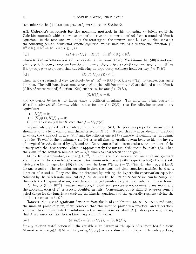
remembering the 〈·〉 notations previously introduced in Section 2.

A.2. Galerkin's approach for the moment method. In this appendix, we brie�y recall theGalerkin approach which allows to properly derive the moment method from a standard kineticequation. In the next one, we apply the strategy to the mixture model. Let us then considerthe following general collisional kinetic equation, whose unknown is a distribution function f :R3 × R∗+ × R3 → RI , with I ≥ 1, i.e.

(40) ∂tf + v · ∇xf = K(f) on R3 × R∗+ × R3,

where K is some collision operator, whose domain is named D(K). We assume that (40) is endowedwith a strictly convex entropy functional, namely, there exists a strictly convex function η : RI →R ∪ {+∞}, y 7→ η(y), such that the following entropy decay estimate holds for any f ∈ D(K):

(41) 〈K(f),∇yη(f)〉I ≤ 0.

Then, in a very standard way, we denote by η∗ : RI → R ∪ {−∞}, z 7→ η∗(z), its convex conjugatefunction. The collisional invariants associated to the collision operator K are de�ned as the kinetic(I-list of tensor-valued) functions X(v) such that, for any f ∈ D(K),

〈X,K(f)〉I = 0,

and we denote by kerK the linear space of collision invariants. The most important feature ofK is the extended H-theorem, which states, for any f ∈ D(K), that the following properties areequivalent:

(i) K(f) = 0;(ii) 〈∇yη(f),K(f)〉I = 0;(iii) there exists φ ∈ kerK such that f = ∇zη∗(φ).

In particular, joined to the entropy decay estimate (41), the previous properties mean that fshould tend to a local equilibrium characterized by K(f) = 0 when there is no gradient. In practice,however, the transport term v · ∇xf and the collision one K(f) compete, depending on the regimeat stake. To exhibit the dominant term, let us recall that the gradient term behaves like the inverseof a typical length, denoted by 1/`, and the Boltzmann collision term scales as the product of thedensity with the cross section, which is approximately the inverse of the mean free path 1/λ. Thenthe value of the Knudsen number Kn = λ/` allows to characterize the regime.

At low Knudsen number, i.e. Kn ≤ 10−3, collisions are much more important than any gradientand, following the extended H-theorem, the zeroth-order term (with respect to Kn) of any f sat-isfying the kinetic equation (40) should have the form f0(t, x, ·) = ∇zη∗(φx,t), where φx,t ∈ kerKfor any x and t. The remaining question is then the space and time equations satis�ed by φ as afunction of x and t. They can �rst be obtained by writing the hyperbolic conservation equationsatis�ed by the zeroth order moment of f . Subsequently, the �rst-order correction can be computedthanks to the Chapman-Enskog procedure and we get parabolic equations involving di�usive terms.

For higher (than 10−3) Knudsen numbers, the collision process is not dominant any more, andthe approximation of f0 as a local equilibrium fails. Consequently, it is di�cult to guess some apriori shape for the functions satisfying the kinetic equation, and this generally requires solving thefull kinetic equation itself.

However, the case of signi�cant deviation from the local equilibrium can still be computed usingthe moment point of view, if we consider that this method provides a practical and theoreticalapproach to compute Galerkin solutions to the kinetic equation itself [41]. More precisely, we saythat f is a weak solution to the kinetic equation (40) when

(42) 〈ψ, ∂tf〉I + 〈ψ, v · ∇xf〉I = 〈ψ,K(f)〉I ,for any relevant test-function ψ in the variable v. In particular, the space of relevant test-functionsM must satisfy ∇yη(f) ∈M, so that, using ∇yη(f) as a test-function in (42) and the entropy decay


for the collision term (41), the following estimate holds for the weak solution

〈∇yη(f), ∂tf〉I + 〈∇yη(f), v · ∇xf〉I ≤ 0.

The Galerkin method consists in considering an increasing sequence of subspaces kerK = M0 ⊂M1 ⊂ · · · such that cl(∪Mk) = M (where cl stands for the closure topologic operator) and to takeany of the �nite dimensional subspaces Mk, k ∈ N, as the test-function space in (42), that is, forany ψ ∈Mk,

(43) 〈ψ, ∂tf〉I + 〈ψ, v · ∇xf〉I = 〈ψ,K(f)〉I , with ∇yη(f) ∈Mk.

We need to brie�y recall the presentation performed in [34] to understand the method. The entropycondition for f implies that we can look for f under the form f(t, x, v) = ∇zη∗(ϕk(v)), where ϕklies in Mk. Let us then consider M(v) be a basis of Mk, that is M(v) = (M1(v), · · · ,Mp(v)). Anelement of Mk can be written as A ·M (v). Looking for f is thus equivalent to look for the functionsA(t, x) as the space-time component of the function ∇yη(f) in the space Mk. Alternatively, de�nethe moment associated to f as

R(t, x) = 〈M, f(t, x, ·)〉I = (〈M1,∇zη∗(A(t, x) ·M)〉I , · · · , 〈Mp,∇zη∗(A(t, x) ·M)〉I).

This is the so-called entropic change of variable: there is a one-to-one correspondence between R(t, x)and A(t, x). In order to help the reader with the thermodynamical interpretation of the unknownsR, A, let us emphasize that, in the context of the so-called thermodynamics of irreversible processes,when Mk = M0 = kerK, the following facts are standard.

• The unknown Re(t, x) stores any of the extensive quantities which are conserved, which arenot a�ected by the collision process.• The unknown Ae(t, x) stores any of the so-called intensive conjugate conserved quantities.• The unknown Me(v) stores the extensive kinetic functions associated to the conserved quan-tities.

The elements of the triplet (Re,Ae,Me(v)) are linked in a unique way thanks to the relationship

Re = 〈Me,∇zη∗(Ae ·Me)〉I .

In the non-equilibrium context, we wish to keep the vocabulary of extensive moment (R) and intensiveconjugate moment (A). The correspondence between extensive and conjugate intensive moments isestablished thanks to the study of the convex function

h(A) = 〈η∗(A ·M)〉I ,

for which we can also de�ne the associated conjugate convex function h∗. For any moment R =(r1, · · · , rp), we write

h∗(R) = supA

[(p∑

k=1

ak : rk

)− h(A)

], with A = (a1, · · · , ap).

When things go round (in particular, h needs to be strictly convex), for any well-chosen R, there isa unique A such that A = Arg sup(h∗(R)). It can be computed thanks to the Euler condition

(44) R−∇Ah(A) = 0⇔ R = 〈M,∇zη∗(A ·M)〉I .

This establishes the one-to-one correspondence between R and A, which can be �nally written usingthe functions h and h∗:

R(A) = ∇Ah(A), A(R) = ∇Rh∗(R).

Hence, going back to our Galerkin problem, looking for the function f speci�ed by both conditionsfrom (43) leads us to eventually �nd the moments R(t, x) associated to f in the kinetic spaceMk. Themoments can be searched by solving the moment equation associated to the Galerkin approximation.


Now, with [34], assume that f is a Galerkin approximation of the solution to the kinetic equation(40), that is we impose

f(t, x, ·) = ∇zη∗(A(t, x) ·M).

The weak formulation for the Galerkin problem (43) now reads

〈M, ∂tf〉I + 〈M, v · ∇xf〉I = 〈M,K(f)〉I ,f(t, x, ·) = ∇zη∗(A(t, x) ·M).

If we introduce the notations

S(A) = 〈M,K(∇zη∗(A ·M))〉I , J(A) = 〈v⊗M · A,∇zη∗(A ·M)〉I ,we formally obtain

∂tR +∇x · J(A) = S(A).

Using the one-to-one correspondence between A and R, thanks to the strictly convex functions h,h∗, the previous equation can be rewritten as

∂tR +∇AJ(∇Rh∗(R))D2

RRh∗(R)∇xR = S(∇Rh

∗(R)).

Such an equation is known as the Friedrich-Lax form of the hyperbolic system, see [34]. Then, ifthis equation has a solution, the Galerkin problem also has a solution.

A.3. Application to the mixture case. The Galerkin approach for the Boltzmann equation (3)was derived for a single monatomic gas, yielding (at the �rst level out of equilibrium) the so-calledLevermore 14-moments. It has been computed with success [31, 32] as an alternative to the Navier-Stokes equations with slip boundary conditions or DSMC simulations in Couette �ow at moderateKnudsen numbers. This seems to con�rm the idea that the moment method enables to reach kineticsystems that tend to escape from local equilibrium. Up to our knowledge, the moment method hashardly been applied in the mixture case, see [39]. The method is roughly described in Appendix A.2in a quite general setting. In order to apply the formalism in our situation, let us �rst write a fewformal properties of the mixture kinetic model.

The entropy associated to the Boltzmann equations for mixtures (3) is given, for any y ∈ RI , by

(45) η(y) =

I∑i=1

yi ln(yi)− yi if y ∈ (R∗+)I ,

+∞ in all other cases.

We obviously have, for any y ∈ (R∗+)I ,

∇yη(y) = (ln(y1), · · · , ln(yI))ᵀ.

Besides, the associated conjugate convex function η∗ satis�es, for any z ∈ RI ,

η∗(z) =

I∑i=1

ezi ,

which immediately implies that, for any z ∈ RI ,∇zη∗(z) = (ez1 , · · · , ezI )ᵀ.

Using the following notations, for any v,

N1(v) =

10...0

, · · · ,NI(v) =

0...01

,


C1(v) =

m1v

0...0

, · · · ,CI(v) =

0...0

mIv

, E(v) =1

2

m1v

2

m2v2

...mIv

2

,the space M0 = kerQ for the mixture collision operator Q(f, f) satis�es, as stated in [12],

(46) M0 = Span(N1, · · · ,NI ,∑i

Ci,E).

Note that we already pointed out the importance of (Ci) in Proposition 2 to compute the Maxwell-Stefan di�usion coe�cients. In the sequel, we also consider

(47) M1 = Span(N1, · · · ,NI ,C1, · · · ,CI ,E).

We clearly have M0 ⊂M1.Let us now consider the entropy density function h : M1 → R given by

h(A) = η∗(A ·M(v)) =

I∑i=1

exp ([A ·M(v)]i),

where M (v) is the tensorially formulated basis of M1 and where we have, as previously de�ned, forany i,

[A ·M(v)]i =

p∑k=1

ak : [Mk(v)]i.

This function h takes its values in R ∪ {+∞}, and its domain domh is, by de�nition, the set of allA such that h(A) is �nite. That exactly requires that the intensive conjugate moment on the energycolumn tensor E(v) is negative. Moreover, thanks to the regularity of η∗, h is regular, and we cancompute, at any point of the open set domh, the derivative of h, i.e., for any A ∈ domh, and anyk ∈ J1, pK,

[∇Ah(A)]k =I∑i=1

〈[Mk(v)]i,∇zη∗([A ·M(v)]i)〉.

Thanks to the properties of η∗, h is a strictly convex function, and we have, for any A, and anyindices k and `,

(48) [D2AAh(A)]k` =

I∑i=1

〈[Mk(v)]i ⊗ [M`(v)]i, D2zzη∗([A ·M(v)]i)〉.

By strict convexity of η∗, D2zzη∗ is a symmetrical positive bilinear form, and consequently, (48)

implies that D2AAh(A) is also a symmetrical positive bilinear form.

Consider now a so-called realizable moment R = (R0, · · · ,Rp). It means that there exists avector-valued kinetic function f = (f1, · · · , fI), with nonnegative components, such that, for anyk ∈ J0, pK,

(49) Rk = 〈Mk(v), f〉I =

I∑i=1

〈[Mk(v)]i, fi〉.

Then it can be argued that the set of all realizable moments is included in the domain of h∗.Moreover, for any realizable moment R, the unique maximizer of h∗(R) is obtained for A satisfyingthe Euler condition R = ∇Ah(A), which is recalled in (44) in Appendix A.2. As a consequence, wecan compute a moment equation in M1 associated to the Boltzmann equation. Moreover, inverting,for any x and t, the extensive moment variable R(t, x) into the intensive conjugate variable A(t, x),


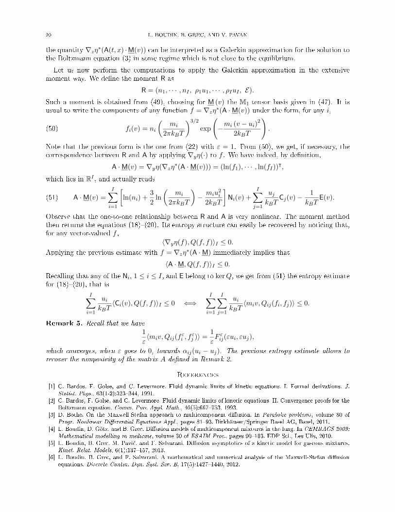
the quantity ∇zη∗(A(t, x) ·M(v)) can be interpreted as a Galerkin approximation for the solution tothe Boltzmann equation (3) in some regime which is not close to the equilibrium.

Let us now perform the computations to apply the Galerkin approximation in the extensivemoment way. We de�ne the moment R as

R = (n1, · · · , nI , ρ1u1, · · · , ρIuI , E).

Such a moment is obtained from (49), choosing for M (v) the M1-tensor basis given in (47). It isusual to write the components of any function f = ∇zη∗(A ·M(v)) under the form, for any i,

(50) fi(v) = ni

(mi

2πkBT

)3/2

exp

(−mi (v − ui)2

2kBT

).

Note that the previous form is the one from (22) with ε = 1. From (50), we get, if necessary, thecorrespondence between R and A by applying ∇yη(·) to f . We have indeed, by de�nition,

A ·M(v) = ∇yη(∇zη∗(A ·M(v))) = (ln(f1), · · · , ln(fI))ᵀ,

which lies in RI , and actually reads

(51) A ·M(v) =

I∑i=1

[ln(ni) +

3

2ln

(mi

2πkBT

)− miu

2i

2kBT

]Ni(v) +

I∑j=1

ujkBT

Cj(v)− 1

kBTE(v).

Observe that the one-to-one relationship between R and A is very nonlinear. The moment methodthen returns the equations (18)�(20). Its entropy structure can easily be recovered by noticing that,for any vector-valued f ,

〈∇yη(f), Q(f, f)〉I ≤ 0.

Applying the previous estimate with f = ∇zη∗(A ·M) immediately implies that

〈A ·M, Q(f, f)〉I ≤ 0.

Recalling that any of the Ni, 1 ≤ i ≤ I, and E belong to kerQ, we get from (51) the entropy estimatefor (18)�(20), that is

I∑i=1

uikBT

〈Ci(v), Q(f, f)〉I ≤ 0 ⇐⇒I∑i=1

I∑j=1

uikBT

〈miv,Qij(fi, fj)〉 ≤ 0.

Remark 5. Recall that we have

1

ε〈miv,Qij(f

εi , f

εj )〉 =

1

εF εij(εui, εuj),

which converges, when ε goes to 0, towards αij(ui − uj). The previous entropy estimate allows to

recover the nonposivity of the matrix A de�ned in Remark 2.

References

[1] C. Bardos, F. Golse, and C. Levermore. Fluid dynamic limits of kinetic equations. I. Formal derivations. J.Statist. Phys., 63(1-2):323�344, 1991.

[2] C. Bardos, F. Golse, and C. Levermore. Fluid dynamic limits of kinetic equations. II. Convergence proofs for theBoltzmann equation. Comm. Pure Appl. Math., 46(5):667�753, 1993.

[3] D. Bothe. On the Maxwell-Stefan approach to multicomponent di�usion. In Parabolic problems, volume 80 ofProgr. Nonlinear Di�erential Equations Appl., pages 81�93. Birkhäuser/Springer Basel AG, Basel, 2011.

[4] L. Boudin, D. Götz, and B. Grec. Di�usion models of multicomponent mixtures in the lung. In CEMRACS 2009:

Mathematical modelling in medicine, volume 30 of ESAIM Proc., pages 90�103. EDP Sci., Les Ulis, 2010.[5] L. Boudin, B. Grec, M. Pavi¢, and F. Salvarani. Di�usion asymptotics of a kinetic model for gaseous mixtures.

Kinet. Relat. Models, 6(1):137�157, 2013.[6] L. Boudin, B. Grec, and F. Salvarani. A mathematical and numerical analysis of the Maxwell-Stefan di�usion

equations. Discrete Contin. Dyn. Syst. Ser. B, 17(5):1427�1440, 2012.


[7] L. Boudin, B. Grec, and F. Salvarani. The Maxwell-Stefan di�usion limit for a kinetic model of mixtures. ActaAppl. Math., 136:79�90, 2015.

[8] L. Boudin and F. Salvarani. Compactness of linearized kinetic operators, Nov. 2015. Review article, preprint.[9] J.-F. Bourgat, L. Desvillettes, P. Le Tallec, and B. Perthame. Microreversible collisions for polyatomic gases and

Boltzmann's theorem. European J. Mech. B Fluids, 13(2):237�254, 1994.[10] M. Briant. Stability of global equilibrium for the multi-species Boltzmann equation in L∞ settings. ArXiv e-prints,

Mar. 2016.[11] M. Briant and E. Daus. The Boltzmann equation for a multi-species mixture close to global equilibrium. ArXiv

e-prints, Jan. 2016.[12] S. Brull, V. Pavan, and J. Schneider. Derivation of a BGK model for mixtures. Eur. J. Mech. B Fluids, 33:74�86,

2012.[13] H. K. Chang. Multicomponent di�usion in the lung. Fed. Proc., 39(10):2759�2764, 1980.[14] L. Chen and A. Jüngel. Analysis of a multidimensional parabolic population model with strong cross-di�usion.

SIAM J. Math. Anal., 36(1):301�322, 2004.[15] X. Chen and A. Jüngel. Analysis of an incompressible Navier-Stokes-Maxwell-Stefan system. Comm. Math. Phys.,

340(2):471�497, 2015.[16] C. F. Curtiss. Symmetric gaseous di�usion coe�cients. J. Chem. Phys., 49(7):2917�2919, 1968.[17] E. S. Daus, A. Jüngel, C. Mouhot, and N. Zamponi. Hypocoercivity for a linearized multispecies Boltzmann

system. SIAM J. Math. Anal., 48(1):538�568, 2016.[18] L. Desvillettes, T. Lepoutre, and A. Moussa. Entropy, duality, and cross di�usion. SIAM J. Math. Anal.,

46(1):820�853, 2014.[19] L. Desvillettes, R. Monaco, and F. Salvarani. A kinetic model allowing to obtain the energy law of polytropic

gases in the presence of chemical reactions. Eur. J. Mech. B Fluids, 24(2):219�236, 2005.[20] J. B. Duncan and H. L. Toor. An experimental study of three component gas di�usion. AIChE Journal, 8(1):38�

41, 1962.[21] A. Fick. Ueber Di�usion. Ann. der Physik, 170:59�86, 1855.[22] V. Garzó, A. Santos, and J. J. Brey. A kinetic model for a multicomponent gas. Phys. Fluids A, 1(2):380�383,

1989.[23] V. Giovangigli. Convergent iterative methods for multicomponent di�usion. Impact Comput. Sci. Engrg.,

3(3):244�276, 1991.[24] V. Giovangigli. Multicomponent �ow modeling. Modeling and Simulation in Science, Engineering and Technology.

Birkhäuser Boston Inc., Boston, MA, 1999.[25] F. Golse and L. Saint-Raymond. The Navier-Stokes limit of the Boltzmann equation for bounded collision kernels.

Invent. Math., 155(1):81�161, 2004.[26] T. Graham. Researches on the arseniates, phosphates, and modi�cations of phosphoric acid. Phil. Trans. R. Soc.

Lond., 123:253�284, 1833.[27] H. Hutridurga and F. Salvarani. On the Maxwell-Stefan di�usion limit for a mixture of monatomic gases. ArXiv

e-prints, Sept. 2015.[28] A. Jüngel. The boundedness-by-entropy method for cross-di�usion systems. Nonlinearity, 28(6):1963�2001, 2015.[29] A. Jüngel and I. V. Stelzer. Existence analysis of Maxwell-Stefan systems for multicomponent mixtures. SIAM

J. Math. Anal., 45(4):2421�2440, 2013.[30] R. Krishna and J. A. Wesselingh. The Maxwell-Stefan approach to mass transfer. Chem. Eng. Sci., 52(6):861�911,

1997.[31] P. Le Tallec and J.-P. Perlat. Numerical analysis of Levermore's moment system. Research Report RR-3124,

Inria, 1997. Projet M3N.[32] P. Le Tallec and J. P. Perlat. Boundary conditions and existence results for Levermore's moments system. Math.

Models Methods Appl. Sci., 10(1):127�152, 2000.[33] T. Lepoutre, M. Pierre, and G. Rolland. Global well-posedness of a conservative relaxed cross di�usion system.

SIAM J. Math. Anal., 44(3):1674�1693, 2012.[34] C. D. Levermore. Moment closure hierarchies for kinetic theories. J. Statist. Phys., 83(5-6):1021�1065, 1996.[35] Y. Lou and S. Martínez. Evolution of cross-di�usion and self-di�usion. J. Biol. Dyn., 3(4):410�429, 2009.[36] Y. Lou and W.-M. Ni. Di�usion, self-di�usion and cross-di�usion. J. Di�erential Equations, 131(1):79�131, 1996.[37] J. C. Maxwell. On the dynamical theory of gases. Phil. Trans. R. Soc., 157:49�88, 1866.[38] I. Müller and T. Ruggeri. Rational extended thermodynamics, volume 37 of Springer Tracts in Natural Philosophy.

Springer-Verlag, New York, second edition, 1998. With supplementary chapters by H. Struchtrup and Wolf Weiss.[39] M. Pavi¢-�oli¢ and S. Simi¢. Moment closure hierarchies for rare�ed gases. Theor. Appl. Mech., 42(4):261�276,

2015.[40] J. Perrin. Mouvement brownien et réalité moléculaire. Ann. Chim. Phys., 123:5�104, 1909.[41] J. Schneider. Entropic approximation in kinetic theory. M2AN Math. Model. Numer. Anal., 38(3):541�561, 2004.


[42] L. Schwartz. Les tenseurs. Hermann, Paris, second edition, 1981. Suivi de �Torseurs sur un espace a�ne�. [With�Torsors on an a�ne space�] by Y. Bamberger and J.-P. Bourguignon.

[43] N. Shigesada, K. Kawasaki, and E. Teramoto. Spatial segregation of interacting species. J. Theoret. Biol.,79(1):83�99, 1979.

[44] J. Stefan. Ueber das Gleichgewicht und die Bewegung insbesondere die Di�usion von Gasgemengen. Akad. Wiss.

Wien, 63:63�124, 1871.[45] F. Williams. Combustion Theory. Benjamin Cummings, second edition edition, 1985.

L.B.: Sorbonne Universités, UPMC Univ Paris 06, CNRS, INRIA, Laboratoire Jacques-Louis Lions(LJLL CNRS UMR 7598), Équipe-projet Reo, Paris, F-75005, France

E-mail address: [email protected]

B.G.: MAP5, CNRS UMR 8145, Sorbonne Paris Cité, Université Paris Descartes, FranceE-mail address: [email protected]

V.P.: Aix-Marseille Université, CNRS, IUSTI UMR 7343, F-13013 Marseille, FranceE-mail address: [email protected]

the maxwell-stefan diffusion limit for a kinetic model of

Documents