the materiality and neutrality of neutral density and
TRANSCRIPT

The Materiality and Neutrality of Neutral Density and Orthobaric Density
ROLAND A. DE SZOEKE AND SCOTT R. SPRINGER*
College of Oceanic and Atmospheric Sciences, Oregon State University, Corvallis, Oregon
(Manuscript received 1 May 2008, in final form 2 February 2009)
ABSTRACT
The materiality and neutrality of neutral density and several forms of orthobaric density are calculated and
compared using a simple idealization of the warm-sphere water mass properties of the Atlantic Ocean.
Materiality is the value of the material derivative, expressed as a quasi-vertical velocity, following the motion
of each of the variables: zero materiality denotes perfect conservation. Neutrality is the difference between
the dip in the isopleth surfaces of the respective variables and the dip in the neutral planes. The materiality
and neutrality of the neutral density of a water sample are composed of contributions from the following: (I)
how closely the sample’s temperature and salinity lie in relation to the local reference u–S relation, (II) the
spatial variation of the reference u–S relation, (III) the neutrality of the underlying reference neutral density
surfaces, and (IV) irreversible exchanges of heat and salinity. Type II contributions dominate but have been
neglected in previous assessments of neutral density properties. The materiality and neutrality of surfaces of
simple orthobaric density, defined using a spatially uniform u–S relation, have contributions analogous to
types I and IV, but lack any of types II or III. Extending the concept of orthobaric density to permit spatial
variation of the u–S relation diminishes the type I contributions, but the effect is counterbalanced by the
emergence of type II contributions. Discrete analogs of extended orthobaric density, based on regionally
averaged u–S relations matched at interregional boundaries, reveal a close analogy between the extended
orthobaric density and the practical neutral density. Neutral density is not superior, even to simple orthobaric
density, in terms of materiality or neutrality.
1. Introduction
It has been a century since the demonstration of the
relation of ocean currents to density gradients (Helland-
Hansen and Nansen 1909). The data from the Meteor
expedition (Wust 1935) showed the close alignment of
core layers in the ocean, on which water properties like
salinity, dissolved oxygen, etc., assumed extremal values,
with strata of density corrected, however crudely, for
adiabatic compression. [Usually, st was used, which is
merely the in situ density with its pressure dependence
neglected; occasionally, the specific volume anomaly has
been employed (Reid 1965).] Montgomery (1938) gave a
cogent, qualitative explanation of why water properties
should spread out along (corrected) density surfaces.
For a long time, potential density was accepted as the
correct standard for comparison with water property
core layers, but Lynn and Reid (1968) showed a sen-
sitive and anomalous dependence of the topography
of potential density surfaces on the choice of their
reference pressure. The distortion of these surfaces
complicates the relationship between potential density
gradients and dynamically important pressure gradients
(de Szoeke 2000). This is most dramatically illustrated
by the well-known reversal of the vertical gradient of
the potential density (referenced to zero pressure) in a
stably stratified region of the deep Atlantic Ocean. The
cause can be traced to the fact that the effective thermal
expansion coefficient of potential density is that of the
in situ density at the potential density’s reference pres-
sure, thereby incorrectly representing thermal effects on
buoyancy at pressures far from the reference pressure
(McDougall 1987b). To mitigate this shortcoming, po-
tential density has been computed over narrow pres-
sure ranges (e.g., 0–500, 500–1500, 1500–2500 dbar, etc.),
referenced to pressures within the respective ranges
(s0, s1, s2, etc.) and matched at the transition pres-
sures to form composite surfaces (Reid and Lynn 1971).
* Current affiliation: Earth and Space Research, Seattle,
Washington.
Corresponding author address: Roland A. de Szoeke, 104A
COAS Administration Bldg., Oregon State University, Corvallis,
OR 97331.
E-mail: [email protected]
AUGUST 2009 D E S Z O E K E A N D S P R I N G E R 1779
DOI: 10.1175/2009JPO4042.1
� 2009 American Meteorological Society
A further elaboration allows for geographical variation
by matching different values of potential density across
the transition pressures in different regions. This pro-
cedure [sometimes called the patched potential density
method (de Szoeke and Springer 2005)] has been used
successfully (e.g., Reid 1994) to create global-scale
maps of potential temperature and salinity, radio tracers
such as tritium corrected for its radio decay, anthropo-
genic tracers like chlorofluorocarbons, or nutrients like
nitrate and phosphate corrected for oxygen concentra-
tion [so-called NO and PO (Broecker 1981)].
The formulation of the patched potential density is
not entirely satisfactory (de Szoeke and Springer 2005).
A significant limitation is that it is defined discretely in
both the vertical and horizontal directions. The vertical
discretization was refined by de Szoeke and Springer
(2005), who showed that decreasing the vertical pressure
interval of the patches from the typical 1000 to 200 dbar,
say, may render the matching procedure ill-defined
because there is no longer a one-to-one correspon-
dence between potential density surfaces across re-
gional boundaries. Two major definitions of continuous
corrected density variables have been proposed: neutral
density (Jackett and McDougall 1997) and simple or-
thobaric density (de Szoeke et al. 2000). These two var-
iables seem, at least superficially, to be very different.
Part of the goal in this paper is to derive them within a
common framework so that their relationship can be
understood more easily. A second goal is to compare
their performance in idealized settings that are analyt-
ically tractable. We propose three quantitative stan-
dards for comparison: 1) How material are the surfaces
of the variable? 2) How closely do the gradients of the
variable correspond to dynamically important density
gradients? 3) How neutral are surfaces of the variable?
The first two standards are motivated directly by early
discoveries about the relationship between thermo-
dynamic variables and motion, and the third is moti-
vated by considerations of the preferred directions of
mixing. These concepts will now be defined precisely.
Strict materiality is the quality of being material, or
conservative:1 a fluid variable is material (conservative)
if it does not change following the motion, or Dx/Dt 5 0.
Quasi-materiality is the property of a variable changing
only in response to irreversible, diabatic effects; that is,
Dx=Dt 5 _qx [ $ � (K$x), where K is a diffusivity tensor
for the variable. In this paper, by materiality we shall
mean (at very slight risk of confusion) quasi-materiality.
This is not to imply that irreversible contributions to the
balance of x are negligible, only that reversible contri-
butions to strict materiality are under consideration.
Potential temperature and potential density (with a
single reference pressure) are material variables. How-
ever, in situ density r governed by the balance
Dr
Dt5 c�2 Dp
Dt1 _qr, where c�2 5
›r
›p
����u,S
, (1.1)
is not material because of reversible adiabatic com-
pression, apart from irreversible effects _qr.
Though not material, density (or specific volume
V 5 r21) has the following crucial substitution property
for the combination that occurs in the equations of
motion of pressure gradient force and gravitational ac-
celeration:
�r�1$p� gk 5�$V
M(V) � k9(V)[›V
M(V) � p],
(1.2)
where M(V) 5 Vp 1 gz is the Montgomery function
(closely related to dynamic height) of density surfaces
and k9(V) 5 (k 2 $Vz)/›Vz.2 The exact replacement, as
it were, of 2r21$p by the three-dimensional gradient
of M(V), expressed relative to nonorthogonal slanting
nonunit basis vectors i, j, and k9(V), and of 2gk by pk9(V)
in the vertical component, is of crucial consequence to
the balance of forces regarded from isopycnal surfaces
(de Szoeke 2000). The effective buoyant force acts in
the direction of k9(V) 5 $V, that is, normal to isopycnals.
When the left side of (1.2) is set equal to the Coriolis
force, this substitution becomes the basis of the thermal
wind calculation of the dynamic height and geostrophic
currents: M(V) 5Ð
p dV (Sverdrup et al. 1942). Taking
the vertical component of the curl of the momentum
balance relative to isopycnal coordinates furnishes a
potential vorticity based on the spacing of in situ iso-
pycnals. The balance of this potential vorticity is
marred, however, by very strong vortex stretching due
to motions across in situ density surfaces arising from
adiabatic compression.
1 It has been traditional in physical oceanography to denote as
conservative what we call here material. Because the former has
recently been used in a rather different sense (McDougall 2003),
we have adopted the latter term.
2 Notation conventions: $p 5 $zp 1 k›zp and $zp 5 i›xjzp 1
j›yjz p, where ›xjz p 5 pxjz, ›yjz p 5 pyjz, etc., are partial derivatives
at fixed z; ›zp 5 pz, etc., are partial derivatives with respect to z;
i, j, k are orthogonal unit basis vectors, horizontal and vertical; $Vz 5
i›xjVz 1 j›yjVz is the gradient of isopycnal surfaces; ›xjVz 5 zxjV,
›yjVz 5 zyjV, etc., are partial derivatives at constant V; ›Vz 5 zV, etc.,
are partial derivatives with respect to V; and $VM(V) 5 i›xjVM(V) 1
j›yjVM(V) is the two-dimensional vector gradient at constant V of the
Montgomery function M(V). Similar usages with independent vari-
ables other than V will be employed.
1780 J O U R N A L O F P H Y S I C A L O C E A N O G R A P H Y VOLUME 39
The density of seawater is a function of potential
temperature, salinity, and pressure. If there were a
temperature–salinity relation unvarying in space or time
in the oceans, density could be regarded as a function
only of pressure and potential temperature u: r21 5
V(p, u). In that case the pressure gradient plus gravi-
tational acceleration combination occurring in the
momentum balance may be replaced by the following:
�r�1$p � gk 5�$uM(u) � [›
uM(u) � P(u)]k9(u),
(1.3)
where M(u) 5 gz 1 H(u) is the Montgomery function, the
sum of the gravitational potential and heat content, the
latter defined by H(u) 5Ð p
0 V(p, u)dp; P(u) 5 [›H(u)/›u]p
is the Exner function; and k9(u) 5 (k 2 $uz)/›uz 5 $u.
This has obvious parallels to (1.2), with similar inter-
pretations. The potential vorticity based on u-surface
(isentrope) spacing ›uz is far more attractive than the
r-surface potential vorticity because the potential tem-
perature is material and the dientropic vortex stretching
is much reduced or negligible (Eliassen and Kleinschmidt
1954). Also, the potential temperature gradient $u is
parallel to the dianeutral vector,
d 5 r�1(�$r 1 c�2$p) (1.4)
(about which more will be developed below), when
there is an unvarying temperature–salinity relation.
Isentropes in this situation are neutral surfaces. This
property is closely linked to the material property of
potential temperature.
The nexus among the three properties of potential
temperature—dynamical substitution (1.3), materiality,
and neutrality—is broken when the temperature–salinity
relation is not unvarying but dependent on geographic
location. In such a case the dianeutral vector d cannot
be parallel everywhere to any scalar gradient, let alone
$u, though it may be taken to define at any point a
neutral plane to which it is perpendicular. An early
hope was that the totality of neutral planes would de-
fine a generalization of neutral surfaces, but this does
not happen (McDougall 1987a; Davis 1994). The for-
mation of well-defined surfaces from neutral planes
requires that their helicity vanish everywhere; that is,
d � $ 3 d 5 0. This amounts to demanding an unvary-
ing temperature–salinity relation, which brings us back
to isentropes, closing the logical circle! Failing this,
global measures of the closeness to neutral planes of the
isopleth surfaces of a given variable can be devised—
which could be called the surfaces’ neutrality. For ex-
ample, Eden and Willebrand (1999) considered several
global indices of the mean-square difference, variously
weighted, between slopes of candidate surfaces and the
neutral plane slope. A variable that labels such candi-
date surfaces may be called a neutral density of the first
kind.
Simple orthobaric density s4—a function only of
density and pressure, and called simple to distinguish it
from extended orthobaric density, considered below
(section 5)—is calculated by assuming a virtual com-
pressibility r21c0(r, p)22—also a function only of pres-
sure and density—to correct the in situ density for
compression: u ds4 5 dr 2 c0(r, p)22 dp, where u(r, p)
is an integrating factor. De Szoeke et al. (2000) fitted
a function of p and r to the global field of sound speed
in the ocean to furnish c0(r, p). This was shown to be
equivalent to fitting a global average u–S relation. Be-
cause it depends only on the in situ density and pres-
sure, the simple orthobaric density has the dynamical
property (1.3), with s4 substituted for u. The material
derivative of s4 may be calculated (de Szoeke and
Springer 2005). The simple orthobaric density is not
material unless the true sound speed c is identical with
the hypothetical c0 everywhere; that is, unless the as-
sumed u–S relation actually applies everywhere. The
difference c0 2 c is a measure of the materiality of the
orthobaric density. A normalized index c of material-
ity, called the buoyancy gain factor, was devised for
simple orthobaric density. This factor is so called be-
cause it gives the ratio of the apparent buoyancy fre-
quency squared, based on the orthobaric density, to the
true buoyancy frequency squared. Its difference from
1 is proportional to c0 2 c and is, thereby, a measure of
the ocean’s deviation from the hypothetical universal
u–S relation. One of the tasks of this paper is to quan-
tify the neutrality of the simple orthobaric density
(section 4). Another task is to explore how using spa-
tially variable u–S relations to define the extended or-
thobaric density affects materiality and neutrality
(section 5).
Jackett and McDougall (1997) described how to
compute a variable g, which they called neutral density,
constructed in such a way that its isopleth surfaces3 are
closely tangent to neutral planes everywhere. Given,
say, a synoptic hydrographic section, the method cal-
culates apparent displacements of water samples on the
section from a standard global reference dataset, such as
the Levitus climatology, and associates neutral density
values preassigned to the reference data to the synoptic
samples. One of the goals of this paper is to clarify the
3 Neutral density and its isopleth surfaces are well defined, even
when neutral surfaces do not exist (i.e., nonzero helicity). We will
be careful to refer to neutral density surfaces, not neutral surfaces.
AUGUST 2009 D E S Z O E K E A N D S P R I N G E R 1781

definition of this neutral density, designated here as the
second kind, and, in particular, to distinguish it from
neutral density of the first kind. McDougall and Jackett
(2005a) proposed measures of materiality and neutral-
ity for neutral density (section 2), modeled on de
Szoeke et al.’s (2000) work with orthobaric density.
However, we will show that in their calculation of
neutral-density materiality a consequential term was
unjustifiably neglected, and their conclusions about the
relative materiality of neutral density and orthobaric
density (McDougall and Jackett 2005b) are suspect. In
addition, we quantify the neutrality of the neutral den-
sity for the first time and derive an expression for the
additional forces that arise on neutral density surfaces,
which do not possess the substitution property (1.3) (see
the appendix).
The plan of this paper is as follows. In section 2
we briefly review how the neutral density of a water
sample is calculated relative to a reference global hy-
drographic dataset. In the appendix, we calculate the
material derivative of neutral density. We also derive a
formula for the difference between the slopes and ori-
entations of neutral density surfaces and neutral
planes (neutrality), and a generalization of the dynam-
ical substitution property (1.3) for neutral density.
In section 3 we take as the reference dataset for neutral
density a simple model of the Atlantic that represents
the ocean’s meridional variation of the u–S rela-
tion, though constructed in such a way that in situ iso-
pycnals are level and the reference ocean is motionless.
Supposing the ‘‘real’’ ocean to have been vertically
displaced from the reference ocean by meridionally
varying amounts, we calculate, by methods analogous to
Jackett and McDougall’s (1997), the distribution of
neutral density and its material derivative. In section 4
we calculate the simple orthobaric density, based on
a mean u–S relation of the reference dataset, of the
displaced real ocean, as well as its material derivative
and neutrality, which we compare to those of neutral
density. We also calculate the dual-hemisphere ortho-
baric density (de Szoeke and Springer 2005), where
different mean northern and southern u–S relations
representative of the respective hemispheres are em-
ployed. We show how the two different simple or-
thobaric densities in the hemispheres may be patched
together. In an extension of these ideas, by subdividing
the ocean into more and more provinces, each with its
distinctive mean u–S relation, and eventually passing to
the obvious continuous limit, we obtain what we have
called the extended orthobaric density (section 5),
whose properties can be compared to those of neutral
density. A discussion and summary conclude the paper
(section 6).
2. Neutral density
a. Preliminaries
In what follows it is useful to have the following
definitions and concepts at hand. The equation of state
r21 5 V(p, u, S) is a function of pressure, potential tem-
perature, and salinity (Jackett et al. 2006). The dianeutral
vector defined by (1.4) may also be written
d 5 a$u� b$S, where a 5 V�1(›V/›u)p,S
and
b 5�V�1(›V/›S)p,u
(2.1)
(McDougall 1987a). Its vertical component is k � d 5 N2/g
(where k is a unit vertical vector, g is the earth’s gravi-
tational acceleration, and N is the buoyancy frequency)
and a, b are the thermal expansion and haline contraction
coefficients. The dip of a neutral plane, or neutral dip, is
the two-dimensional vector whose direction in the hori-
zontal gives the orientation of the plane, and whose
magnitude is the tangent of the angle between the neutral
plane and the horizontal, namely,
h 5(d 3 k) 3 k
k � d 5�d 1 (k � d)k
k � d 5�a$
zu 1 b$
zS
a›zu� b›
zS
.
(2.2)
[This usage is common in describing bedding planes in
physical geology (Holmes 1945).] The dianeutral vector
is integrable, that is, d 5 u$n, so that h 5 2$zn/›zn 5
$nz, if and only if the helicity vanishes:
d � $ 3 d 5�m*$p � a$u 3 b$S 5 0, (2.3)
where m* 5 ›ln (a/b)/›p. The latter has typical recipro-
cal values for seawater of m2 1* ’ 5000 dbar (McDougall
1987b; Akitomo 1999; Eden and Willebrand 1999).
Condition (2.3) is satisfied if S 5 S(u, p). In that case,
surfaces of constant n are everywhere tangential to
neutral planes (perpendicular to d) and may be properly
called neutral surfaces. The dynamical substitution (1.3)
is valid, with n substituted for u. (Under the slightly
more restrictive condition S 5 S(u), n may be taken to
be identical to u, as was assumed in the introduction.)
Various practical kinds of neutral density have been
devised even when (2.3) is not satisfied. But the tangent
planes of their surfaces cannot perforce be perpendic-
ular everywhere to the dianeutral vector, so estimates of
their closeness to this ‘‘ideal’’ ought to be formed. This
is one of the tasks undertaken in the following.
b. Neutral density of the first kind
Suppose we call $gz the dip of a surface z 5 z(g, x), as
labeled by the constant parameter g. The vector dif-
ference between this dip and the neutral dip,
1782 J O U R N A L O F P H Y S I C A L O C E A N O G R A P H Y VOLUME 39

$gz� h, (2.4)
is called the neutrality of the surface. Its magnitude
j$gz 2 hj gives the angle between the surface and the
neutral plane. When the neutrality is zero, surfaces of
constant g are said to be neutral. Even if not, we shall
call these surfaces neutral density surfaces of the first
kind and call g the neutral density,4 when $gz ’ h, to
some acceptable degree of approximation. Several ways
of approximating this equality have been described.
One way is to integrate
›z[g, x(s)]/›s 5 h � x9(s)/ x9(s)j j, (2.5)
where s is the distance along a horizontal path x(s), to
form a three-dimensional neutral trajectory x(s), z(g, s).
By repeating this over a network of such paths chosen to
cover the entire ocean, and ‘‘connecting’’ paths sharing
the same value of g, McDougall (1987a) suggested that
‘‘approximate surfaces’’ may be formed. There are un-
avoidable mathematical difficulties with this approach
when the helicity of the dianeutral vector does not
vanish (Davis 1994). However, a realizable approach is
to choose z(g, x) to minimize the neutrality globally,
that is, to minimize
ðV
jW � ($gz� h)j2 dV, (2.6)
where V is the total volume of the ocean and W is a
suitable weight function. Eden and Willebrand (1999)
considered several similar minimization principles. Neu-
tral density surfaces of the first kind exist even when the
neutrality $gz 2 h differs from zero. They must be re-
garded, however, as one step removed from neutral
planes.
c. Neutral density of the second kind
It is impractical to recalculate the global neutral
density field whenever a new hydrographic section be-
comes available. Accordingly, Jackett and McDougall
(1997) described a two-stage procedure for assigning the
value of a second kind of practical neutral density to a
sample of water collected at a certain horizontal posi-
tion and ambient pressure.
(i) The first stage is to prepare beforehand a set of
reference neutral density surfaces of the first kind
from an archive of hydrographic data, such as the
Levitus climatology, from which averaged vertical
reference profiles of potential temperature and sa-
linity, uref(p, x), Sref(p, x),5 at any position x in the
world’s oceans have been compiled. (One might call
this the reference ocean.) The reference surfaces
are specified by the function
p 5 pref
(g, x) [or its inverse, g 5 gref
(p, x)].
(2.7)
(ii) Next, suppose a water sample has been collected
with the values u, S at ambient pressure p, position
x, and time t, from the present ocean (so called to
distinguish it from the reference ocean). The target
pressure level pr is the pressure at which the refer-
ence ocean’s potential density matches the present
sample’s potential density, each referenced to the
weighted-average p 5 l~p 1 lpr [with l~ 1 l 5 1;
Jackett and McDougall (1997) invariably use l 5
l~ 5 0.5 for the weights]. This prescription may be
written as
V[p, uref
(pr, x), Sref
(pr, x)] 5 V(p, u, S) (2.8)
and is called the neutral property (Jackett and
McDougall 1997). It furnishes pr as a function of
u, S, p, and position x. The last step is to obtain
the neutral density of the second kind of the water
sample by substituting pr into the predetermined
function gref(pr, x).
Graphically, this identifies the reference neutral
density surface that goes through the target level pr at
position x in the reference ocean, and associates its
neutral density (first kind) with the present water sam-
ple. This second kind of neutral density is two steps
removed from neutral planes: first by the association the
neutral property [Eq. (2.8)] makes between the present
ocean and the reference ocean, and second by the re-
lation of the reference neutral density to neutral planes.
d. Material rate of change: Cross-neutral mass flow
An important property of neutral density of the
second kind can be obtained by taking the material
derivatives6 of both sides of Eqs. (2.8) and (2.7) and
eliminating Dpr/Dt to furnish an equation for its material
4 Surfaces may be labeled alternatively by any G(g). It is con-
venient to resolve this ambiguity by setting g to the potential
density at a central location (e.g., Jackett and McDougall 1997).
5 We prefer to use pressure p rather than height z as a vertical
coordinate.6 The material derivative operator is given by any of the fol-
lowing: D/Dt 5 ›tjz 1 u � $z 1 w›z 5 ›tjp 1 u � $p 1 _p›p 5 ›tjg 1
u � $g
1 _g›g, etc., where w 5 _z 5 Dz/Dt, _p 5 Dp/Dt, _g 5 Dg/Dt,
etc.; ›tjz, etc., are partial time derivatives with z, etc., held constant.
This invariance to reference frame is demonstrated by de Szoeke
and Samelson (2002).
AUGUST 2009 D E S Z O E K E A N D S P R I N G E R 1783

rate of change, _g [ Dg/Dt, in the present ocean. (De-
tails are given in the appendix.) We call the value of _g at
a point in space and time the materiality; if the mate-
riality were zero everywhere, g would be perfectly
material, or conservative. Materiality gives the rate of
flow eg (m s21, positive when upward) across neutral
density surfaces. This is obtained in the appendix by
Eq. (A.2), which is reproduced here:
�rgeg [ _g›p
›g5 (cg � 1)[l~(›
t1 u � $)
gp 1 lu � $
gpr]|fflfflfflfflfflfflfflfflfflfflfflfflfflfflfflfflfflfflfflfflfflfflfflfflfflfflfflfflfflfflfflfflfflffl{zfflfflfflfflfflfflfflfflfflfflfflfflfflfflfflfflfflfflfflfflfflfflfflfflfflfflfflfflfflfflfflfflfflffl}
I
1 l~m(p� pr)D�1u � $gq
ref|fflfflfflfflfflfflfflfflfflfflfflfflfflfflfflfflfflfflfflfflffl{zfflfflfflfflfflfflfflfflfflfflfflfflfflfflfflfflfflfflfflfflffl}II
1 D�1 N2ref
g�
$g
pr
rref
g� h
ref
� �� u
|fflfflfflfflfflfflfflfflfflfflfflfflfflfflfflfflfflfflfflfflfflfflfflfflffl{zfflfflfflfflfflfflfflfflfflfflfflfflfflfflfflfflfflfflfflfflfflfflfflfflffl}III
1 D�1 _q( p)|fflfflfflffl{zfflfflfflffl}
IV
. (2.9)
In this equation, cg 5 1� m[q� qref(pr, x)]D�1 is the
neutral-density buoyancy gain factor;7 q, s are normal-
ized forms of u, S (slightly nonlinearly transformed in
the case of q; see the appendix); m 5 Vup/Vu is the
thermobaric parameter (McDougall 1987b); D is a fac-
tor given by (A4) in the appendix; and Ds›p/›g is the
vertical thickness (in pressure units, i.e., decibars) of an
increment Ds of neutral density. The right side of (2.9)
uses a simplified equation of state given by Eqs. (A.1a)
and (A.1b) in the appendix.
One may distinguish four types of contributions to the
material rate of change, or the diapycnal material flow,
arising from the following sources:
(I) the sum of the apparent vertical motion in the
present ocean, wa 5 (›t 1 u � $)g p, as though the
constant-g surface were material, and in the ref-
erence ocean, wra 5 u � $g pr (Fig. 1), each weighted
by l~ or l, respectively, and attenuated by cg � 1,
which is a measure of the departure of the water
sample’s q, s from the local reference u–S relation;
(II) differences between ambient pressure in the pres-
ent data and target pressure in the reference da-
taset, p 2 pr, combined with advection of the
reference temperature on neutral density surfaces
(if the reference temperature changes on the ref-
erence neutral density surfaces, it is because of
the spatial variation of the reference ocean’s u–S
relation);
(III) reference neutrality, that is, differences between
the neutral density surface dip $gzref 5 2$g pr/
(rrefg) and the true neutral dip href (see the ap-
pendix) in the reference dataset; and
(IV) the irreversible rates of change of temperature
and salinity that constitute the buoyancy rate of
change _q( p) [see Eq. (A5) in the appendix].
e. Neutrality
Another result established in the appendix is an
equation for the neutrality, the difference in the present
ocean between the dip $gz of the neutral density (of the
second kind) and the neutral dip h. This difference is
given by Eq. (A.9):
N2
g($
gz� h) 5 D(cg � 1)$
g(l~p 1 lpr)|fflfflfflfflfflfflfflfflfflfflfflfflfflfflfflfflfflfflfflffl{zfflfflfflfflfflfflfflfflfflfflfflfflfflfflfflfflfflfflfflffl}
I
1 m(p� pr)$g(l~q
ref1 lq)|fflfflfflfflfflfflfflfflfflfflfflfflfflfflfflfflfflfflfflfflfflffl{zfflfflfflfflfflfflfflfflfflfflfflfflfflfflfflfflfflfflfflfflfflffl}
II
1N2
ref
g�
$g
pr
rref
g� h
ref
� �|fflfflfflfflfflfflfflfflfflfflfflfflfflfflfflfflffl{zfflfflfflfflfflfflfflfflfflfflfflfflfflfflfflfflffl}
III
. (2.10)
One may identify contributions analogous to types I, II,
and III for materiality. Note the distinction between the
FIG. 1. Neutral density schematic. Two neutral density surfaces,
g and g9 5 g 1 Ds, are shown in the (top) ‘‘present’’ dataset (at two
times: t and t 1 Dt) and (bottom) in the reference dataset (fixed).
The distinction between the present thickness p9 2 p 5 Ds›p/›g
and the reference thickness p9r 2 pr 5 Ds›pr/›g is illustrated. Ap-
parent vertical motions in the present dataset, wa 5 (›t 1 u � $)g p,
and in the reference dataset, wra 5 u � $g pr [using a horizontal
current from the present data at p, x, t (or g, x, t)], are indicated.
7 McDougall and Jackett (2005a) define cg � 1 5 l(cg � 1),
which is convenient when l 5 l~ 5 0.5 is used.
1784 J O U R N A L O F P H Y S I C A L O C E A N O G R A P H Y VOLUME 39
neutralities of the present ocean (left-hand side) and the
reference ocean (term III).
McDougall and Jackett (2005b) derived an expres-
sion similar to (2.9). Jackett and McDougall (1997)
argued that, given their method of preparing the ref-
erence dataset, the type III term in (2.9) [and by in-
ference in (2.10)] is small. McDougall and Jackett
(2005a) conducted a global census of cg from the world
hydrographic dataset showing that it is very close to
1 (q 2 qref ’ 0) and concluded that the type I contri-
bution to the materiality (and, one may infer, neutrality)
of neutral density due to deviations from the local u–S
relation is negligibly small. Further, following from a
claim that m(q 2 qref)u � $g pr (type I) and m(p 2 pr )u �$gqref (type II) were typically of the same order, they
asserted that diapycnal flow contributions from spa-
tial gradients of the reference u–S relation were like-
wise negligible. This claim is very dubious. In section 3
we shall present an illustration clarifying that type II
contributions to neutrality and materiality cannot be
neglected.
f. Neutral density in the displaced reference ocean
The treatment in the appendix is quite general with
regard to the reference dataset and the present ocean. A
special case is of particular interest. Suppose the present
ocean is obtained from the reference ocean by displac-
ing the latter vertically by an increment Dp, possibly
itself a function of p, x, and t:
q 5 qref
(p 1 Dp, x), and s 5 sref
(p 1 Dp, x). (2.11)
When this is substituted into the right side of (2.8), an
obvious solution for target pressure is
pr 5 p 1 Dp. (2.12)
Hence, q 2 qref(pr, x) 5 0 and cg 5 1 exactly, so that
the type I terms in the materiality and neutrality of
neutral density, Eqs. (2.9) and (2.10), vanish. But the
type II terms, proportional to p 2 pr 5 2Dp 6¼ 0, do not.
3. Properties of neutral density in anidealized ocean
To evaluate the performance of neutral density (and,
in section 4, orthobaric density) with regard to materi-
ality and neutrality, it is useful to consider a simplified
model of the Atlantic Ocean’s meridional temperature
and salinity structure that illustrates its salient hydro-
graphic features. This model will be taken as the ref-
erence dataset for the neutral density algorithm. Its
motivation is the spatial dependence of the Atlantic’s
u–S relation, which was identified in the preceding sec-
tions as the cause of nonzero helicity and the nonexis-
tence of neutral surfaces. We will suppose the present
ocean to be a vertically displaced form of the reference
ocean from which we can calculate the neutral density
distribution and its materiality and neutrality.
a. A simple model of the warm-waterAtlantic Ocean
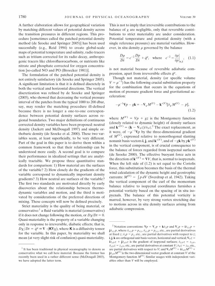
The u–S relation of the Atlantic on the horizontal
500-dbar pressure surface is shown in Fig. 2 in terms of
the modified variables q, s [Eq. (A1b) in the appendix].
The diagram shows the main southern and northern
lines of the tropical to temperate upper ocean, with a
constant-density bridge linking the main lines. The
nonlinear transformation of potential temperature u has
straightened a slight curvature of the lines. On any
pressure surface shallower than 1500 dbar [only 500
dbar is shown here, but see de Szoeke and Springer
(2005) for more pressure surfaces], the main lines are
practically identical, while the bridge lies at different
densities. The two fitted lines in Fig. 2,
s 5 R�1q 7 s1, with R ’ 2.0 (density ratio) and
s1’ 0.23 3 10�3, (3.1)
may be considered idealized representations of the main
u–S lines at temperatures above 48C (q $ 20.11 3 1023).
FIG. 2. The u–S relation of the Atlantic on the 500-dbar pressure
surface. The ordinate is q: shifted, transformed, and normalized
potential temperature. The abscissa is normalized and shifted sa-
linity. The grayscale clouds represent data points taken from the
World Ocean Circulation Experiment (WOCE). The coefficients
and parameters a1, a2, b, u0, S0, given in the appendix, are chosen so
that unit changes in q or s give unit changes in the normalized
specific volume V/V0. The solid lines are analytic representations
of the main southern and northern u–S lines; their slopes are R 5
dq/ds 5 2.0. The dashed line is a constant-density line linking the
main lines at 500 dbar.
AUGUST 2009 D E S Z O E K E A N D S P R I N G E R 1785

More elaborate representations of the u–S lines than
(3.1), taking account of the convergence of the northern
and southern lines at colder temperatures, may readily
be considered, though in the interests of brevity we have
foregone such a treatment here. It may be more con-
ventional to show the spatial variation of u–S relations as
in Fig. 3, where each line of data represents a meridional
location. This illustrates the evolution along a meridional
section from the southern to the northern extremes ide-
alized in Eq. (3.1). The near-constant density bridge
structure at each pressure, exemplified in Fig. 2, unfolds
to form the meridionally dependent u–S profiles of Fig. 3.
The fit of parallel, straight lines to the q–s relation at
each latitude for waters warmer than 48C or shallower
than 1500 dbar seems quite accurate. The lines are biased
to the saltier side on passing from 208S to 208N, but are
unvarying with latitude south and north, respectively, of
these limits (overlooking some anomalously salty water
from the Mediterranean at northern midlatitudes). A
linear fit to this bias between 208S and 208N may be
oversimplified but not unrepresentative.
Thus, Figs. 2 and 3 motivate the following idealiza-
tions of the temperature and salinity fields of the
warmer layers of the subtropical to tropical Atlantic:
qref
(p, y) 5d
ref( p) 1 ( y/L)s
1
n 1 mp, and (3.2a)
sref
(p, y) 5 (1 1 mp)qref
(p, y)� dref
(p), (3.2b)
for jy/Lj # 1, where y 5 6L are the northern and
southern geographical boundaries of the transequatorial
Atlantic bridge region. For y/L . 11 ( y/L , 21), we
replace y/L in (3.2a) by 11 (21). We take 2L ’ 3000 km
and n 5 1 2 R21 ’ 0.5. (The origin, y 5 0, need not be
the equator.) The qref and sref fields are chosen to give a
horizontally uniform profile of the normalized specific
volume anomaly,
dref
( p) 5�s9B
p, (3.2c)
here assumed linear with depth with constant coefficient
s9B. We call this the quiescent reference ocean (Fig. 4).
One might as well assign the d values of level pressure
surfaces (or rather their negatives) as the neutral den-
sity labels of the reference ocean, that is, as in Eq. (2.7):8
gref
(p, x) 5�dref
( p) 5 s9B
p. (3.2d)
If dref is eliminated from (3.2a) and (3.2b), a meridio-
nally variable reference q–s relation emerges:
sref
5 R�1qref
1 (y/L)s1, where y/Lj j # 1 (3.2e)
(cf. Fig. 3). The q–s relations at successive positions
from y 5 2L to L are straight lines of slope R, shifting
to saltier water. The total shift is 2s1. South of y 5 2L
(or north of y 5 L) the q–s relation is taken to be
spatially uniform, as given by Eq. (3.1). The end-point
northern and southern q–s relations, though very sim-
ple, represent the real ocean very well, as does the
mapping of the intermediate q–s relations onto the
FIG. 3. Profiles of u vs S at fixed latitudes on a meridional section
of the Atlantic (grayscale lines). (See Fig. 2 caption and the ap-
pendix for coefficients and parameters.) The variation is greatest
between 158S and 158N. At higher latitudes, the northern and
southern u–S relations are nearly constant. The idealized northern
and southern u–S relations in Fig. 2 are shown.
FIG. 4. A cross section of u (solid) and S (dashed) in a simple
model of the quiescent warm-water Atlantic. The in situ isopycnals
are level.
8 More generally, if the in situ density surfaces of the reference
dataset were not level, the reference neutral density surfaces
would depend on position, g 5 gref(pr, x) (see the appendix).
1786 J O U R N A L O F P H Y S I C A L O C E A N O G R A P H Y VOLUME 39

constant-density bridges (Fig. 2). More schematic than
strictly accurate is the assumption of a meridionally
linear transition between the end points (Fig. 3).
A consequence of the density-compensated bridge
structure [Eq. (3.2)] is that in situ isopycnals and neutral
planes (McDougall 1987a) are horizontal in the refer-
ence dataset. The dianeutral vector [Eq. (2.1)] is ev-
erywhere vertical,
dref
5 krref
g[s9B
1 mqref
(p, y)] 5 kg�1N2ref(p, y); (3.2f)
hence, the reference helicity is trivially zero: dref � $ 3
dref 5 0. The reference neutrality is also zero; the refer-
ence state exactly (and trivially) satisfies 2$gpr/(rrefg) 5
href 5 0, so that the type III terms that occur in (2.9)
and (2.10) are absent. Reference-neutral surfaces are
level.
From Eq. (3.2) describing the quiescent reference
state, one obtains
N2ref
rref
g25 s9
B1 mq
ref’ s9
B,
›pr
›g5
1
s9B
,
›qref
›pr5�s9
B� mq
ref
n 1 mpr’�
s9B
n,
$gq
ref5 j
s1/L
n 1 mpr’ j
s1
nL,
8>>>>>>>>>><>>>>>>>>>>:
(3.3)
where j is the meridional unit vector. [When approxi-
mations are given in (3.3), the contributions from the
small parameter m have been neglected.]
b. Idealized neutral density in the displacedreference ocean
Let the place of the hydrographic archive used as the
reference data for the neutral density algorithm (2.8) be
taken by the two-dimensional quiescent reference state
[Eq. (3.2)]. Suppose that the present ocean is the ref-
erence ocean displaced by Dp(p, x), as in Eqs. (2.11). In
general, then, helicity will not be zero and neutral sur-
faces will not exist. However, neutral density and its
isopleth surfaces are well defined and can be obtained
by inserting Eq. (2.11) on the left of (2.8). As remarked
above, the target pressure pr is then given by (2.12), and
the neutral density by
g 5 s9B
pr 5 s9B
(p 1 Dp).
Neutral density surfaces are described by pr 5 const.
Interesting properties of neutral density, such as mate-
riality and neutrality, may be estimated. The buoyancy
gain factor for the displaced ocean is cg 5 1 (because
q 2 qref(pr, x) 5 0), and type I terms in (2.9) and (2.10)
vanish. In a pressure range centered around 500 dbar
(for p , p0 ; 1000 dbar, say), suppose the displacement
is linear in x and y:
Dp ’ D0(«x/L 1 y/L 1 1)/2, (3.4)
with D0 5 100 m. The dominant, type II, contribution to
Eq. (2.9) is, using (3.3),
egII ’
l~m
rgs9B
Dpys
1
nL’ l~
ms1
rgns9B
LyD
0(y/L 1 1)/2.
(3.5)
The parameter « in (3.4) may be so small as to be neg-
ligible in Dp in (3.5), but it is essential in providing a
nonzero meridional velocity y 5 f21s9B(p 2 p0)D0«/2L
to make (3.5) nonzero and nontrivial. Fundamentally,
the zonal structure of (3.4) provides three-dimensional
structure in the displaced ocean to furnish nonzero
helicity. The meridional dependence of this is shown in
Fig. 5a for l~ 5 0.5, normalized by a parameter including
the meridional velocity y.
The neutrality of neutral density is given by Eq. (2.10).
Applying this formula to the displaced reference ocean,
in which only the type II term on the right survives, one
obtains, using the approximations of (3.3),
$gz� h ’�j
mDp
rgs9B
s1
nL’�j
ms1D
0
rgns9B
L(y/L 1 1)/2.
(3.6)
This difference, or mismatch, is shown in Fig. 5b. Cu-
riously, even if « [ 0, despite the displaced ocean’s
being perfectly two-dimensional with zero helicity (so
that neutral surfaces are well defined), the neutrality of
neutral density surfaces does not vanish. An estimate
of the dimensionless parameter appearing in both (3.5)
and (3.6) is
m
nrg
s1
L
D0
s9B
’(5000 dbar)�1
(0.5)(1 dbar m�1)
(0.23 3 10�3)
(1500 km)
3(100 dbar)
(0.6 3 10�6 dbar�1)’ 1.1 3 10�5.
This gives eg ; 1025 y ; 1027–1026 m s21 for y ;
1022–1021 m s21. In comparison to typical Ekman pump-
ing magnitudes near the ocean surface (;1026 m s21),
such dianeutral material flows are not inconsiderable.
4. Properties of orthobaric density in anidealized ocean
The idealized representation in section 3 of the
Atlantic Ocean illustrates well the central irremediable
AUGUST 2009 D E S Z O E K E A N D S P R I N G E R 1787

feature of the ocean’s density field that gives nonzero
helicity: the spatial variation of the u–S relation. We
now turn to calculating orthobaric density functions
predicated on u–S relations from various locations in the
reference ocean. These relations and density functions
are summarized in Table 1. We also calculate their
buoyancy gain factors (Table 2), cross-isopleth mass
flows (materiality), and neutrality (difference of the
surfaces’ $z from neutral dip h), and compare them with
those for neutral density.
a. Simple orthobaric density
An orthobaric density function for the entire ideal-
ized Atlantic may be defined in the following way. Take
the reference q–s relation (3.2e) at some central loca-
tion, say y 5 0, that is, sref 5 R21qref. By (3.2a), qrefjy50
is related to a normalized specific volume anomaly d
[Eq. (A1a) in the appendix] and pressure p by
qrefjy50
5d
n 1 mp.
FIG. 5. (top) The type II contribution to diapycnal mass flow egII [Eq. (2.9)] for neutral density
(dashed), and the type I contribution to diapycnal mass flow e4I [Eq. (4.2)] for simple (global)
orthobaric density (solid), with both normalized by ms1/(ns9B)yD0/(Lrg). (bottom) Neutrality
for neutral density [difference (mismatch) between the dip of the surfaces and the neutral dip;
see Eq. (2.10)] (dashed), and for simple (global) orthobaric density [Eq. (4.5)] (solid), nor-
malized by ms1/(ns9B)D0/Lrg.
TABLE 1. Orthobaric density functions.
q–s (q–d) relation Orthobaric density
Global ( y 5 0) sref 5 R�1qref [qref j0 5 d(n 1 mp)�1] s4 5�d
1 1 mp/n
Northern ( y 5 L) sref 5 R�1qref 1 s1 [qrefjL 5 (d 1 s1)(n 1 mp)�1] sN 5 m(L)�1 �d� s1
1 1 mp/n1 s1
� �
Southern ( y 5 2L) sref
5 R�1qref� s
1[q
refj�L
5 (d� s1)(n 1 mp)�1] sS 5 m(�L)�1 �d 1 s1
1 1 mp/n� s
1
� �
Arbitrary center (yj) sref
5 R�1qref
1 s1y
j/L
[qref jyj5 (d 1 s1yj/L)(n 1 mp)�1]
s(yj) 5 m(yj)
�1�d� s1yj/L
1 1 mp/n1 s1yj/L
� �
Note: m(y) 5 1 1ms1y
ns9B
L
1788 J O U R N A L O F P H Y S I C A L O C E A N O G R A P H Y VOLUME 39

By substituting this into the adiabatic compressibility
anomaly (›d/›p)q,s 5 mq, one obtains the virtual com-
pressibility anomaly, which may be used to pose the
following differential equation:
dd
dp5 mq
refjy50
5md
n 1 mp.
This furnishes the integral 2d/(1 1 mp/n) 5 const. One
may take the value of this ‘‘constant,’’ defining a surface
in d, p space, at a reference pressure, say p 5 0, to be s4.
In this way one obtains a simple ‘‘global’’ orthobaric
density9 as a function of d, p:
s4 5�d
1 1 mp/n. (4.1)
The material rate of change of s4 may be calculated. It
can be written as
�rge4 [ ›p/›s4 _s4 5 (c4 � 1)(›t1 u � $)
s4 p|fflfflfflfflfflfflfflfflfflfflfflfflfflfflfflfflfflfflfflffl{zfflfflfflfflfflfflfflfflfflfflfflfflfflfflfflfflfflfflfflffl}I
1 ›p/›s4 ~u4c4 _q(p)|fflfflfflfflfflfflfflfflfflfflfflfflfflffl{zfflfflfflfflfflfflfflfflfflfflfflfflfflffl}IV
(4.2)
(de Szoeke et al. 2000; de Szoeke and Springer 2005).
Here, Ds›p/›s4 is the vertical thickness (dbar) of an
increment Ds of orthobaric density. In addition, e4 is
the net flow (m s21) across a s4 isopycnal and consists
of two parts. The first is an adiabatic part—a residual of
the compressibility effect—given by the apparent mo-
tion (›t 1 u � $)s4 p of orthobaric isopycnals, attenuated
by c4 2 1, where
c4 5 f1 1 ~u4m[q� qrefjy50
(s4)]›p/›s4g�1 (4.3)
is the buoyancy gain factor, in which
qrefjy50
(s4) 5�s4/n and
~u4 5�›s4/›d 5 (1 1 mp/n)�1.
Only at the location from which the reference q–s re-
lation has been taken (y 5 0) will q 5 qref in the dis-
placed ocean, and c4 5 1, reducing term I in (4.2) to
zero. The remaining part of (4.2), labeled IV, is a term
proportional to _q( p), the sum of all diabatic, irreversible
influences on the negative buoyancy [Eq. (A5), see the
appendix). We have assigned the terms in (4.2) type
designations based on their appearance analogous to
Eq. (2.9). Note that terms of types II or III do not appear.
The buoyancy gain factor of simple orthobaric density
for the displaced reference ocean is listed in Table 2 and
shown in Fig. 6. Note the linear decrease with y of
c4 2 1. A similar decrease is evident in an Atlantic
meridional section of c4 2 1 (de Szoeke et al. 2000,
their Fig. 11). (Since the reference u–S relation in the
latter calculation was taken from southern waters, there
is a positive bias in the real-world section compared to
the idealized section.) Unlike the type I term in the
neutral density materiality, Eq. (2.9), the contribution
of the term of which this is a factor to material flow
across orthobaric isopycnals does not vanish. Consider
the steady-state estimate of the apparent vertical motion,
(›t 1 u � $)s4 p ’ y(›p/›y)
s4 ’ yD0/2L. The contribution
from the type I term of (4.2) to diapycnal flow is
e4I ’
ms1
rgns9B
LyD
0
y
2L. (4.4)
The meridional dependence of this, normalized by
ms1D0/(rgns9BL)y, is shown in Fig. 5a; also shown is the
meridional average value of je4I j (similarly normalized).
One may compare e4I to e
gII, given by (3.5). Though their
meridional dependences are offset one from the other,
their magnitudes and parameter dependences are sim-
ilar. The latter, egII, was neglected by McDougall and
TABLE 2. Buoyancy gain factors in the displaced reference ocean for various orthobaric density functions.
Global c4 � 1 ’s1m
ns9B
�1, y . L�y/L, yj j, L
1, y , �L
0@
1A ~u4 5 (1 1 mp/n)�1
Northern cN � 1 ’s
1m
ns9B
0, y . L1� y/L, 0 , y , L
� �~uN 5 (1 1 mp/n)�1m(L)�1
Southern cS � 1 ’s1m
ns9B
�1� y/L, �L , y , 00, y , �L
� �~uS 5 (1 1 mp/n)�1m(�L)�1
Arbitrary center (yj) c
j� 1 ’
s1m
ns9B
yj � y
L, jy� y
jj, L/(N � 1) ~u
j5 (1 1 mp/n)�1m(y
j)�1
Extended cO 2 1 ’ 0 ~uO 5 (1 1 mp/n)�1m(y)�1
9 More systematically, de Szoeke et al. (2000) defined a global
orthobaric density function on the basis of a volumetrically aver-
aged compressibility function—equivalent to a volumetrically av-
eraged u–S relation.
AUGUST 2009 D E S Z O E K E A N D S P R I N G E R 1789

Jackett (2005a). From (2.9) and (4.2), egI } cg 2 1 and
e4I } c4 2 1. McDougall and Jackett (2005a) show per-
suasively that cg 2 1� c4 2 1, so that indeed egI� e4I .
In our illustration, in fact, egI [ 0, cg 2 1 [ 0. But
in compensation it must be recognized that egII is not
negligible.
The dip of an orthobaric density surface �$s4 p/(rg)
differs from the neutral plane dip h [Eq. (2.2)] by
�$
s4 p
rg� h 5 (c4 � 1)
$s4 p
rg’�(c4 � 1)h
’ jms
1D
0
ns9B
rgL
y
2L(4.5)
(de Szoeke et al. 2000). The last approximate equality
follows from the first row entry of Table 2, and has a
magnitude similar to the neutrality of neutral density
surfaces [Eq. (3.6)]. See Fig. 5b.
The panels in Fig. 5 illustrate a major result of this
paper. They show typical estimates of diapycnal flow
(materiality) and the neutrality of neutral density and
orthobaric density. The dianeutral material flow eg must
be expected to have magnitudes similar to the ortho-
baric diapycnal flow e4. Likewise, the neutralities of
neutral density and orthobaric density are similar.
b. Regional orthobaric density functions
Orthobaric density functions can be defined specific
to various regions, each predicated on a reference q–s
relation typical of its region. To construct global cor-
rected density surfaces, we must specify how to match
the various density functions across their interregional
boundaries (de Szoeke and Springer 2005). We will il-
lustrate this difficulty with some examples.
1) NORTHERN ORTHOBARIC DENSITY
An orthobaric density might be predicated on the q–s
relation (3.2e) at y 5 L, sref 5 R21 qref 1 s1. This choice
is important because it characterizes the water mass
properties of much of the northern North Atlantic, and
the northern portion of the tropical bridge region. If such
a choice is pursued along the preceding lines, one arrives
at the specification of what might be called the northern
orthobaric density function sN, given in the second row
of Table 1. [Any function of (2d 2 s1)/(1 1 mp/n) might
be chosen for sN. We have chosen a particular linear
function, for a reason that will become clear presently.]
The material derivative of s N gives an equation exactly
like (4.2), involving a buoyancy gain factor cN, defined
like (4.3), with 4 superscripts replaced by N superscripts,
FIG. 6. (top) A dual-hemisphere orthobaric isopycnal for the displaced reference ocean. Note
the discontinuity at y 5 0. Meridional motion will carry material through this discontinuity
(leakage). The dotted line is a surface of simple orthobaric density based on a single global-
average u–S relation. (bottom) Buoyancy gain factor c differences from 1 (Table 2, lines 2 and 3)
(solid) for the joint isopycnal in the top panel. The factor does not account for the material flow
through the discontinuity at y 5 0. The dotted line is the buoyancy gain factor for the simple,
global orthobaric isopycnal (Table 2, line 1).
1790 J O U R N A L O F P H Y S I C A L O C E A N O G R A P H Y VOLUME 39

and with qrefjy5L(sN) given in Table 1. The buoyancy
gain factor cN and the integrating factor ~uN for this
northern orthobaric density are listed in Table 2 for the
displaced reference ocean; cN is shown in Fig. 6.
Buoyancy gain factors on a meridional Atlantic section
based on a northern (and a southern) u–S relation are
shown in de Szoeke and Springer’s (2005) Fig. 13.
2) SOUTHERN ORTHOBARIC DENSITY
All this might be repeated to develop another ortho-
baric density function sS based on the q–s relation in
(3.2e) at the southern end of the tropical bridge, y 5 2L;
that is, sref 5 R21qref 2 s1. This will yield the entry in
the third row of Table 1, a linear function of (2d 1 s1)/
(1 1 mp/n). Again, the material derivative of sS, anal-
ogous to (4.2), may be obtained. [See also de Szoeke
and Springer’s (2005) Fig. 13.]
3) DUAL-HEMISPHERE ORTHOBARIC DENSITY
The constant m factors specifying sN, sS in Table 1
have been chosen so that when the undisplaced refer-
ence bridge specific volume anomaly (SVA) profile
applies, d 5 2s9Bp, the two are numerically identical.
Thus, the overall dual-hemisphere quasi-orthobaric
density function defined by
sO(p, d, y) 5 sN(p, d), for y . 0, and
5 sS(p, d), for y , 0, (4.6)
will be continuous across y 5 0 if the said density profile
pertains there. However, if the density profile differs
from this standard, say, d ’2s9B(p 1 Dp), as in the
displaced ocean of section 2, the difference between the
two expressions of (4.6) on either side of y 5 0 is ap-
proximately (using entries from Table 1)
DsO 5 sO��y501
�sO��y50�
5 [sN(p, d)� s S(p, d)]d’�s9
B( p1Dp)
’�2s1mn�1Dp. (4.7)
(In the approximate equality, higher-order terms in m
are neglected.) This gives a discontinuous displacement
for a sO isopycnal across y 5 0 of
Dz 5DsO
rgs9B
’�2s
1mDp
rgns9B
(deeper on the north side, Dz , 0 when displacement
from the standard profile is upward, or Dp . 0; see
Fig. 6). This discontinuity is a potential site of material
leakage. Given meridional velocity y, there is volume
flux through this discontinuity of 2s1m/(rgns9B)(vDp)y50
(m2 s21, positive when toward lighter water). Divided
by 2L, this gives an equivalent cross-isopycnal mass
flow, averaged over the bridge region, of
eOII ’
2s1m
rgns9B
(yDp)y50
/2L ’s
1mD
0
2rgns9B
L(y)
y50. (4.8)
This will be shown normalized below (see Fig. 8a). This
form is convenient for comparison to (4.4) (it is twice
the average of je4I j), the flow across simple orthobaric
isopycnals (s4 5 const), and to (3.5), the material flow
across neutral density surfaces.
5. Extended orthobaric density
The bridge region need not be split into only two parts,
northern and southern, as for the dual-hemisphere den-
sity function. Suppose the bridge region is subdivided
into a number N of intervals jy� yjj, L/(N � 1), where
yj 5 L(2j�N � 1)/(N � 1) for j 5 1, . . . N. The treat-
ment outlined above for the dual-hemisphere density
function may be applied, with obvious modifications, to
each such subinterval, characterized by the u–S relation
given by (3.2e) at its center, y 5 yj. This leads to the
specification in each subinterval of an orthobaric den-
sity function s(yj) listed in the fourth row of Table 1.
Each such density function has an associated buoyancy
gain factor cj (Table 2). The boundaries between the
subintervals correspond to y 5 0 in the dual-hemisphere
orthobaric density. The cj 21 factors determining the
quasi-materiality of a local orthobaric density, defined
by reference to the local u–S relation, are reduced by a
factor of 1/(N21). The discontinuities, analogous to
(4.7), then occurring at the edges of subintervals,
yj11/2
5 L(2j�N)/(N � 1), are similarly reduced,
DsO 5 [s(yj11)(p, d)� s
(yj)(p, d)]
d’�s9B
( p1Dp)
’�2s1mn�1Dpj
yj11/2
/(N � 1),
but are N21 times more numerous (Fig. 7). Given a
meridional flow y, there will be a mass transport through
each such gap, which, averaged over the spacing be-
tween gaps, 2L/(N21), may be thought of as an equiv-
alent diapycnal flow,
eOII ’
s1m
Lrgns9B
(yDp)jyj11/2
, (5.1)
distributed over the interval jy�yj11/2j,L/(N�1). These
flows are shown in Fig. 8 for N 5 2 (dual-hemisphere
orthobaric density), 4, and 10; also shown are the (me-
ridionally unvarying) averages of |eOI | ; O[1/(N 2 1)] in
each subinterval. In the limit N / ‘, eOII tends to the
continuous line shown in Fig. 8.
AUGUST 2009 D E S Z O E K E A N D S P R I N G E R 1791

An alternative view is gained by starting from the
continuous limit of the arbitrarily centered extended
orthobaric density function (fourth row, Table 1):
sO(d, p, y) 5 s(y)(d, p)
5 m(y)�1 �d� (y/L)s1
1 1 mp/n1 (y/L)s
1
� �. (5.2)
The reference temperature field (3.2a) may be expressed
in terms of this entity as
qref
(sO; y) 5 n�1[�m(y)sO 1 (y/L)s1].
If the ocean were in the quiescent reference state given
by (3.2), then, substituting in (5.2),
sO 5s9
Bp
1 1 mp/n.
Otherwise, in the state displaced by Dp from the qui-
escent,
sO � s9B
p(1 1 mp/n)�1’ s9
BDp. (5.3)
This approximation will be used below.
a. Material derivative
The material rate of change of (5.2) may be written
�rgeO [ _sO›p/›sO 5 (cO � 1)(›t1 u � $)
sO p|fflfflfflfflfflfflfflfflfflfflfflfflfflfflfflfflfflfflfflffl{zfflfflfflfflfflfflfflfflfflfflfflfflfflfflfflfflfflfflfflffl}I
� vs
1m
nL
›p
›sO~uOcO sO
s9B
(1 1 mp/n)� p
� �|fflfflfflfflfflfflfflfflfflfflfflfflfflfflfflfflfflfflfflfflfflfflfflfflfflfflfflfflfflfflfflfflffl{zfflfflfflfflfflfflfflfflfflfflfflfflfflfflfflfflfflfflfflfflfflfflfflfflfflfflfflfflfflfflfflfflffl}
II
1 ›p/›sO ~uOcO _q( p)|fflfflfflfflfflfflfflfflfflfflfflfflfflffl{zfflfflfflfflfflfflfflfflfflfflfflfflfflffl}IV
, (5.4)
where
cO 5 1 1 ~uOm[q� qref
(sO; y)]›p/›sO� �1
,
~uO 5 (1 1 mp/n)�1m(y)�1.
Equation (5.4) gives the rate at which matter crosses a
sO isopycnal. The terms labeled I and IV, a residual
compressibility effect and a diabatic contribution, re-
spectively, are analogous to similar terms in (4.2). For
the displaced reference ocean, it can be easily shown
that q 2 qref(sO; y) 5 0, so that cO 5 1, and the first
FIG. 7. (top) Examples of multilinked orthobaric isopycnals based on u–S relations centered
on multiple intervals for link numbers N 5 4, 10. (The latter has been offset deeper by
100 dbar.) Note the discontinuities at the joints. Meridional motion will carry material through
these discontinuities. The dotted line is the extended orthobaric isopycnal (N / ‘). (bottom)
Buoyancy gain factor differences from 1 or 1.1 for the multilinked isopycnals in the top panel.
These factors do not account for the material flow through the discontinuities. The buoyancy
gain factor for the extended orthobaric isopycnal (dotted) is 1.
1792 J O U R N A L O F P H Y S I C A L O C E A N O G R A P H Y VOLUME 39

term in (5.4) vanishes. The contribution of term II may
be written
eOII ’
m
rgs9B
s1
nLyDp ’
ms1
rgs9B
nLyD
0( y/L 1 1)/2. (5.5)
It is proportional to the meridional motion y, the merid-
ional temperature gradient on sO surfaces ›qref (sO; y)/
›y ’ s1/nL, the thermobaric coefficient m, the reciprocal
buoyancy frequency squared ›p/›sO ~uOcO ’ rg2/N2,
and the displacement Dp from the quiescent state. It
coincides with the continuous limit of (5.1), as shown in
Fig. 8. The neutral density diapycnal flow [Eq. (3.5); see
Fig. 8c] differs only in the factor l~ .
Reviewing the progression from simple global ortho-
baric density to dual-hemisphere orthobaric density, to
N-fold discrete extended orthobaric density (EOB), to
continuous EOB, one sees that type I diapycnal flow,
the sole reversible contributor to diapycnal flow across
simple orthobaric density surfaces, is augmented by a
type II contribution when dual-hemisphere EOB is con-
sidered, of about the same magnitude. As the number
N of subintervals is increased, the type II contributions
supplant the type I contributions, which dwindle in-
versely with N. In the continuous limit, only type II
contributions to the EOB diapycnal flow remain, re-
sembling strongly, other than the factor l~ , the diapycnal
flow for neutral density. McDougall and Jackett (2005a),
while confirming the smallness of the type I contribu-
tions, completely neglected the type II contributions to
neutral density materiality. Their conclusion that neutral
density is superior to orthobaric density in its material
properties rests on this fallacy.
b. Neutrality
The difference between the dips of extended orthobaric
density surfaces and neutral planes can be calculated.
Take the quasi-horizontal gradient of (5.2) on constant
sO surfaces. This gives, after some manipulation,
$sO z� h 5 (cO � 1)($
pz� $
sO z)
1 jg
N2
ms1
nLs9B
[�sO(1 1 mp/n) 1 s9B
p].
(5.6)
For the displaced reference ocean, again cO 5 1, and
(5.3) pertains, so that the last factor in the second term is
2s9BDp; also N2/g ’ rgs9B. Hence,
FIG. 8. Type II diapycnal flow eOII [Eq. (5.1)] for discrete extended orthobaric density,
equivalent to the meridional mass flow through the gaps shown in Fig. 7, and located at the
heavy vertical lines, for several choices of numbers N of links: (top) N 5 2 (dual-hemispheric
orthobaric density), (middle) N 5 4, and (bottom) N 5 10. The continuous limit (N / ‘) of eOII
[Eq. (5.5)] is shown in all panels. Type II neutral density diapycnal flow eneutralII [Eq. (2.9)] is also
shown in the bottom panel. Type I diapycnal flow eOI for extended orthobaric density is shown
for N 5 4, 10. All normalized by ms1/(ns9B)yD0/(Lrg).
AUGUST 2009 D E S Z O E K E A N D S P R I N G E R 1793
$sO z� h ’�j
ms1Dp
rgs9B
nL’�j
ms1
rgs9B
nL
D0
2L
y
L1 1
�.
(5.7)
This is indistinguishable from Eq. (3.6), the neutrality
of neutral density, shown in Fig. 5b. One may compare
it to (4.5), the neutrality of simple global orthobaric
density surfaces, also shown in Fig. 5b. While the me-
ridional dependence is shifted and reversed, the amount
of variation is identical.
6. Summary and discussion
Density is an important variable, not merely as a
tracer, but especially because of its link to motion ac-
celeration through the buoyant force. As in situ density’s
utility as a tracer is limited by its susceptibility to adia-
batic compression, efforts are made to correct for this
effect. This would be uncontroversial if the temperature–
salinity relation of the ocean were unvarying with po-
sition. As this is not so, however, only partial solutions
to the difficulty are possible. This paper has considered
two attempts at such solutions: neutral density and
orthobaric density. The results are judged by a num-
ber of criteria: materiality, the degree to which reversible
contributions (apart from irreversible, diabatic con-
tributions) to the substantial rate of change of the cor-
rected density variable are minimal; neutrality, the
degree to which isopleth surfaces of the variable are
everywhere normal to the dianeutral vector d [Eq.
(1.4)]; and the degree to which buoyancy forces can be
regarded as acting across isopleth surfaces, embodied in
the paradigm of Eq. (1.3) for isentropes when the
temperature–salinity relation is unvarying. These crite-
ria are not independent, as the resemblances of
Eq. (2.10) (neutrality) to (2.9) (materiality) show.
Our approach was analytic. We constructed an ide-
alization of the temperature–salinity structure of the
upper kilometer or more of the Atlantic Ocean, in
which the ocean transitions continuously with latitude
from a southern u–S relation to a northern one. A
simplified equation of state was assumed, though with a
representative, nonzero, thermobaric parameter, Vup/Vu.
For the reference ocean required by Jackett and
McDougall’s (1997) neutral density method, for which
the Levitus climatology is usually adopted, we supposed
a quiescent rest state, though with the said meridional
u–S variations. On the other hand, for the reference u–S
relation required for simple orthobaric density, we took
an intermediate relation between the northern and
southern extremes. For the present ocean, as a test, we
assumed a vertically displaced form (with resulting
motion) of the quiescent state, and computed distribu-
tions of materiality and neutrality for each candidate
variable. While this test does not exhaust the range of
real-world possibilities, it throws light on the relative
performances of the variables.
We compared, in Fig. 5, the material flow (material-
ity) across isopleths of neutral density and simple or-
thobaric density, and the mismatch (neutrality) of the
dips of said surfaces from the neutral dip. In sections 2
and 4, we identified several contributions to each of
these indices: type I, due to divergence of the local u–S
relation from the reference u–S relation, and type II,
from the meridional gradient of the reference u–S re-
lation. Because the meridional variation of the u–S
relation is built into the reference ocean, there is by
construction no type I contribution for neutral density,
though there must be a type II contribution. For simple
orthobaric density, on the other hand, the reference u–S
relation is meridionally unvarying so there is no type II
contribution, although, since the local u–S relation dif-
fers from the reference relation, there must be a type I
contribution. Although their spatial distributions are
different, the respective types of contribution to the
materiality and neutrality of the two variables are sim-
ilar and comparable in magnitude. McDougall and
Jackett (2005a), who reached a different conclusion,
which favored neutral density, did so by overlooking the
type II contributions.
A dual-hemisphere orthobaric density function was
devised (section 4). It takes advantage of the close
hemispheric validity of two different u–S relations:
southern and northern. This permits the local reduction
of type I materiality and neutrality contributions. But a
correspondence between the two distinct orthobaric
density functions must be established in order to con-
nect isopleth surfaces between hemispheres. This is
achieved by supposing meridional continuity when the
ocean is in the reference state. When the ocean is not in
the reference state, discontinuities occur in the surfaces
connected across the interhemispheric boundary (the
equator). These are important because, even apart
from the materiality of the surfaces in the respective
hemispheres, they are sites where matter may pass
through the gaps in the surfaces. This form of ortho-
baric density is notable because it is a model of the two-
hemisphere form of patched potential density (Reid
1994) obtained in the limit when the vertical intervals
(or patches, typically chosen to be 1000 dbar thick in
practice) are infinitesimally small. The patched poten-
tial density has been seminal in the development of
both neutral density (Jackett and McDougall 1997) and
orthobaric density (de Szoeke et al. 2000; de Szoeke
and Springer 2005).
1794 J O U R N A L O F P H Y S I C A L O C E A N O G R A P H Y VOLUME 39

The dual-hemisphere idea can be extended to form
multiregional orthobaric density functions, each chosen
with reference to a local u–S relation, and joined be-
tween neighboring regions by the requirement of conti-
nuity when the ocean is in the reference state (section 5).
Thus, type I materiality can be reduced virtually to
nothing, while the discontinuities among regions, and
the material flow across them, even though individually
reduced, become more frequent. In the limit of a me-
ridionally continuous u–S relation, the latter material
flow is seen to be an analog of the type II cross-material
flow of neutral density. This analogy is quantitative.
Apart from a 50% reduction factor for neutral density
{which can be traced to the choice of a half-and-half
reference pressure [Eq. (2.8)]}, the meridional structure
of the type II materiality is identical.
Though the materiality of a variable is of obvious
utility in interpreting its spatial variation, the funda-
mental significance of neutrality is not so clear. It is
often said that the neutral plane at a specific point (the
plane perpendicular to d at that point) contains the
bundle of trajectories on which a water parcel can begin
to move without change in heat or energy, or that
r21(2$p 1 c2$r) 5 2c2d is the buoyant restoring force
of adiabatic test particle excursions. We cannot sub-
stantiate such statements. Rather, when, for example, a
spatially unvarying u–S relation applies, so that neutral
surfaces exist (and are coincident with isentropes), the
combination of the pressure gradient force and buoy-
ancy force with respect to isentropes may be replaced
by the dynamical relation (1.3), in which the effective
buoyant force is P(u)k9(u) 5 P(u)$u, acting parallel to d.
This is indeed a fundamental property of neutral sur-
faces when they exist. From it, familiar inferences may
be drawn about potential vorticity conservation and
thermal wind balances. The extension or modification of
this property to the case of the spatially varying u–S
relation (so that no neutral surfaces exist) is the perti-
nent dynamical question. We obtained in the appendix
the generalization [Eq. (A.12)], with respect to neutral
density surfaces, of the substitution (1.3), and showed
that there are additional terms—virtual, nonconser-
vative forces in effect—associated with the spatial
variation of the u–S relations implicit in the reference
datasets used in the construction of neutral density.
These additional virtual forces are experienced by water
parcels constrained to follow neutral density surfaces. A
systematic study of the importance of these forces is yet
lacking.
The simple orthobaric density s4 is specifically con-
structed to exhibit under any circumstances the dynam-
ical substitution property (1.3) that isentropes possess
when the u–S relation is unvarying. Nonsimple variants
of orthobaric density will, like neutral density, exhibit
extra virtual forces. For example, on dual-hemisphere
orthobaric density surfaces (based on different northern
and southern u–S relations in each hemisphere of the
globe), which may exhibit discontinuities at the equator,
an impetus proportional to the discontinuity must be
administered to a hypothetical water parcel crossing the
equator to move it to the designated continuation of the
surface. This is analogous to the continuous virtual
forces on neutral density surfaces. Such forces must be
applied to water parcels to keep them moving on con-
tinuous, extended orthobaric density surfaces.
An important question remains about the nature of
orthobaric density and neutral density. It concerns the
sizes of the contributions to materiality that have been
the main subject of this paper—the reversible terms,
principally types I and II—relative to the irreversible,
adiabatic terms (denoted as type IV in sections 2 and 4
and in the appendix). The angle between simple
orthobaric density surfaces and neutral planes has been
estimated on long meridional hydrographic sections
through the Atlantic and Pacific Oceans [see de Szoeke
et al.’s (2000) Fig. 12]. This angle is to very good ap-
proximation the neutrality magnitude j$s4 z� hj calcu-
lated in section 4. De Szoeke et al. (2000) and McDougall
and Jackett (2005a) reached different conclusions about
the significance of the errors incurred in assuming that
the diffusivity tensor’s principal axes are aligned with
orthobaric density surfaces (or neutral density surfaces)
rather than along neutral planes. However, a recent
critical examination of these various alignment hypoth-
eses shows that they are superfluous and makes the di-
vergence of views irrelevant and moot (de Szoeke 2009,
unpublished manuscript).
APPENDIX
Neutral Density
a. Materiality
The general definition of neutral density, Eq. (2.8),
gives the target pressure pr in terms of a water sample’s
values of potential temperature u and salinity S at am-
bient pressure p and horizontal location x, using ar-
chived reference profiles uref and Sref at that location.
Equation (2.7) with pr substituted then gives g. It will be
convenient, though not essential, to use the following
simplified equation of state:
r�1 5 V( p, u, S) 5 V( p) 1 V0d and d 5 (1 1 mp)q� s,
(A.1a)
AUGUST 2009 D E S Z O E K E A N D S P R I N G E R 1795
where
q 5 a1(u� u
0) 1
1
2a
2(u� u
0)2 and s 5 b(S� S
0).
(A.1b)
Here, r is the density, V is the specific volume, d is the
SVA normalized by V0, u is the potential temperature, S
is the salinity, V(p) 5V(p,u0,S
0), and m 5 (Vpu/Vu)p50 ’
2 3 1024 dbar21 is the thermobaric coefficient
(McDougall 1987b).A1 In (A.1b), we used the parameters
u0 5 58C, S0 5 34.63 psu,A2 a1 5 1.13 3 1024 8C21, a2 5
1.35 3 1025 8C22, and b 5 0.799 3 1023 psu21, for the
first and second thermal expansion coefficients, and
the haline contraction coefficient, respectively. The
potential density rr with respect to a fixed reference
pressure r is given by
r�1r 5 V(r, u, S) 5 V(r) 1 V
0[(1 1 mr)q� s]. (A1c)
When the material derivatives of both sides of (2.8)
and (2.7) are taken, and _pr [Dpr/Dt 5 u �$g
pr 1 _g›g
pr
is eliminated, one obtains the following relation among
the material derivative _g of neutral density and _q, _s, _p,
and _x [ u:
�rgeg [ _g›p
›g5 (cg � 1)[l~ (›
t1 u � $)
gp 1 lu � $
gpr]|fflfflfflfflfflfflfflfflfflfflfflfflfflfflfflfflfflfflfflfflfflfflfflfflfflfflfflfflfflfflfflfflfflffl{zfflfflfflfflfflfflfflfflfflfflfflfflfflfflfflfflfflfflfflfflfflfflfflfflfflfflfflfflfflfflfflfflfflffl}
I
1 l~m(p� pr)D�1u � $gq
ref|fflfflfflfflfflfflfflfflfflfflfflfflfflfflfflfflfflfflfflfflffl{zfflfflfflfflfflfflfflfflfflfflfflfflfflfflfflfflfflfflfflfflffl}II
1 D�1 N2ref
g�
$g
pr
rref
g� h
ref
� �� u
|fflfflfflfflfflfflfflfflfflfflfflfflfflfflfflfflfflfflfflfflfflfflfflfflffl{zfflfflfflfflfflfflfflfflfflfflfflfflfflfflfflfflfflfflfflfflfflfflfflfflffl}III
1 D�1 _q( p)|fflfflfflffl{zfflfflfflffl}IV
. (A.2)
The first equality of (A.2) defines the material velocity
eg across surfaces of constant neutral density g; the
Roman numerals identify terms referred to in the main
text; and cg is the buoyancy gain factor for neutral
density, defined by
cg � 1 5�m(q� qref
)D�1, (A.3)
D [N2
ref
rref
g2� l~m(p� pr)
›qref
›pr
� �›pr
›g
�
1 m(q� qref
) l›pr
›g1 l~
›p
›g
� � ›p
›g
� ��1
5N2
rg21 lm(p� pr)
›q
›p. (A.4)
The first equality in (A.4) defines D, while the second
follows from taking the partial g derivative, at constant
x and t, of both sides of Eq. (2.8). Also,
_q( p) [ �(1 1 mp) _q 1 _s
5 (11mp)[�$ � (K$q) 1 a2$u � K � $u] 1 $ � (K$s).
(A.5)
Here, K is the turbulent diffusivity tensor, _q( p) repre-
sents the total effect on the negative buoyancy of irre-
versible exchanges of heat and salt [the superscript ( p)
emphasizes that the normalized thermal expansion
coefficient V�10 ›V/›q 5 1 1 mp, occurring in (A5), is
calculated at pressure p], and a2 5 V210 ›2V/›u2 is the
second expansion coefficient, or cabbeling coefficient,
defined after Eq. (A.1b). In obtaining (A.2) use was
made of identities and definitions such as
_p 5 (›t1 u � $)
gp 1 _g›
gp,
k � dref
rref
g5
N2ref
rref
g25�(1 1 mpr)
›qref
›pr1
›sref
›pr,
(dref
3 k) 3 k 5�(1 1 mpr)$pr qref
1 $pr sref
5 (k � dref
)href
.
8>>>>>><>>>>>>:
(A.6)
Here, qref, sref, Nref, dref are functions of pr and position
x {with rref 5 [V(pr, qref, sref)]21} in the reference ocean,
to be evaluated at pr 5 pref(g, x), while q, s, and N are
functions of p (or g), x, and t in the present ocean. The
equalities in the second and third lines of (A.6) define
the vertical and horizontal components of dref, the dia-
neutral vector in the reference dataset. The last equality
defines the neutral dip href, a vector whose magnitude
and direction in the horizontal plane give the gradient
and orientation, respectively, of neutral planes.
The derivation of (A.2) has as yet used no partic-
ular property of the reference neutral density surfaces.
However, the vanishing, if possible, of the factor in pa-
rentheses of term III in (A.2) (which concerns only fields
from the reference dataset) could be used to provide pr 5
pref(g, x) [or its inverse g 5 gref(pr, x)]. The exact van-
ishing of term III is possible if and only if dref � $ 3 dref 5
0. If this condition is not fulfilled, one may settle for
pref(g, x), which makes term III ’ 0 in some appropriate
global minimal sense (Eden and Willebrand 1999).
A1 More generally, what follows may be readily extended to
cover any equation of state of the form d 5 P( p)q(u, S) 2 s(u, S),
where u and S are the true potential temperature and salinity.A2 Here, psu refers to United Nations Educational, Scientific
and Cultural Organization (UNESCO) Practical Salinity Scale of
1978 (PSS78) salinity units (UNESCO 1981).
1796 J O U R N A L O F P H Y S I C A L O C E A N O G R A P H Y VOLUME 39

Equation (A.2) is similar to an equation derived by
McDougall and Jackett (2005a,b), except that in the first
expression in (A.4) for the factor D these authors in
effect assume that Nref ’ N and ›pr/›g ’ ›p/›g. We
retain the generality of (A.4) because the buoyancy
frequency and spacing of neutral density surfaces may
differ substantially from the reference ocean to the in-
stantaneous present ocean. We have also retained
generality in the choice of weights l and l~ in the ref-
erence pressure p 5 l~p 1 lpr of the potential densities
in Eq. (2.8); this includes McDougall and Jackett’s
(2005a,b) standard setting of l 5 l~ 5 0.5. McDougall and
Jackett’s cg factor is related to (A.3) by
cg � 1 ’ l(cg � 1). (A.7)
One may also see from (A.3) and (A.4) that
cg � 1
q� qref
5�mN2
rg21 lm(p� pr)
›q
›p
� ��1
, (A.8)
which has a limiting value even when q / qref.
One may compare (A.2) to (5.4) for the flow across
extended orthobaric isopycnals. Term I of Eq. (A.2) is
the sum of two terms weighted, respectively, by l~ and l,
and both multiplied by cg 2 1. The first term is the
apparent vertical motion (›t 1 u � $)gp of neutral
density surfaces p 5 p(g, x, t) (as though they were
material) in the present instantaneous dataset. The
second is the apparent vertical motion u � $gpr of neu-
tral density surfaces pr 5 pref(g, x) frozen in the refer-
ence dataset, as though the present instantaneous current
u 5 u(g, x, t) was projected into the reference dataset on
the corresponding neutral density surface (Fig. 1). This
weighted sum of apparent vertical motions seems rather
peculiar. Equation (5.4) contains a counterpart only of
the first of these two contributions. [If the weights
l~ 5 1, l 5 0 were chosen, the correspondence of terms
between (A.2) and (5.4) would be very close.]
Most important, the second term of (5.4) for the
material derivative of the extended orthobaric density
corresponds to the p 2 pr term (II) of (A.2). For
l 5 l~ 5 0.5, using Eq. (A.3) and pz 5 2rg, the first few
terms of Eq. (A.2) become
McDougall and Jackett (2005a) assert that, ‘‘Since
(p 2 pr)u � $gqref is typically of the same order as
(q 2 qref)u � $gpr, all contributions to [Eq. (A.2)9] typi-
cally have the same magnitude.’’ Then, because q 2 qref }
cg 2 1 ’ 0, it would follow that all shown terms, types I
and II, are negligible. However, in the main text we
contest the quoted statement.
b. Neutrality
By taking the gradient along neutral density surfaces
$g of both sides of Eq. (2.8), and making use of the
definitions and identities (A.4) and (A.6), one arrives at
N2
g($
gz� h) 5 �m(q� q
ref)$
g(l~p 1 lpr)|fflfflfflfflfflfflfflfflfflfflfflfflfflfflfflfflfflfflfflfflfflfflffl{zfflfflfflfflfflfflfflfflfflfflfflfflfflfflfflfflfflfflfflfflfflfflffl}
I
1 m(p� pr)$g(l~q
ref1 lq)|fflfflfflfflfflfflfflfflfflfflfflfflfflfflfflfflfflfflfflfflfflffl{zfflfflfflfflfflfflfflfflfflfflfflfflfflfflfflfflfflfflfflfflfflffl}
II
1N2
ref
g�
$gpr
rref
g� h
ref
� �|fflfflfflfflfflfflfflfflfflfflfflfflfflfflfflfflffl{zfflfflfflfflfflfflfflfflfflfflfflfflfflfflfflfflffl}
III
. (A.9)
(The Roman numerals refer to terms discussed in the
main text.) The two quantities in the parentheses on the
left side and in term III on the right of (A.9) are the
neutralities in the present and reference datasets, that is,
the respective differences between the neutral density
surface dip and the neutral plane dip. Even if the
reference neutrality on the right of (A.9) were zero, the
other two terms, particularly the second, proportional to
m(p2pr), may significantly bias the neutrality in the
present dataset.
c. Generalized Montgomery function
Substituting the equation of state (A.1a) into the
neutral property (2.8), one obtains
(1 1 mp)qref
(pr, x)� sref
(pr, x) 5 (1 1 mp)q� s
or
d 5 dref
(pr, x) 1 m(p� pr)[l~qref
(pr, x) 1 lq], (A.10a)
where
dref
(pr, x) 5 (1 1 mpr)qref
(pr, x)� sref
(pr, x), and
pr 5 pref
(g, x). (A.10b)
One may regard Eq. (A.10) as a metaequation of state,
furnishing density as a function of metastate variables g
eg 5 �0.5m (q� qref
)(›t gj p 1 u � $
gp 1 u � $
gpr)|fflfflfflfflfflfflfflfflfflfflfflfflfflfflfflfflfflfflfflfflfflfflfflfflfflfflfflfflfflfflfflfflfflffl{zfflfflfflfflfflfflfflfflfflfflfflfflfflfflfflfflfflfflfflfflfflfflfflfflfflfflfflfflfflfflfflfflfflffl}
I
� (p� pr)u � $gq
ref|fflfflfflfflfflfflfflfflfflfflfflfflfflfflfflffl{zfflfflfflfflfflfflfflfflfflfflfflfflfflfflfflffl}II
8><>:
9>=>;(Dp
z)�1
1 � � � . (A.2)9
AUGUST 2009 D E S Z O E K E A N D S P R I N G E R 1797

and x, in addition to p and q. Defining a generalized
heat content
H(g)(p, g, q, x) 5
ðp
pr
V dp
5
ðp
pr
V( p)dp 1 V0d
ref(pr, x)(p� pr)
11
2V
0m(p� pr)2[l~q
ref(pr, x) 1 lq]
(A.11)
and a generalized Montgomery function M(g) 5 H(g) 1 gz,
one can show that
�r�1$p� gk 5 �$gM(g) 1 Q$
gq 1 X
1 [�›gM(g) 1 Q$
gq 1 P(g)]k9(g),
(A.12)
where k9(g) 5 (k� $gz)/›
gz 5 $g, and
P(g) 5›H(g)
›g
�����p,q,x
5›pr
›g
�����x
›H(g)
›pr
�����p,q,x
, (A.13a)
Q 5›H(g)
›q
�����p,g,x
51
2lV
0m(p� pr)2, (A.13b)
X5$p,q,g
H(g)5$p,pr ,q
H(g)1$gpr›H(g)
›pr
�����p,q,x
,
(A.13c)
›H(g)
›pr
�����p,q,x
5 �V(pr)� V0d
ref(pr, x)
� V0m(p� pr)[l~q
ref(pr, x) 1 lq]
1 V0(p� pr)
›dref
(pr, x)
›pr
11
2l~V
0m(p� pr)2 ›q
ref(pr, x)
›pr, and
(A.13d)
$p, pr , q
H(g) 5 V0(p� pr)$
pr dref(pr, x)
11
2l~V
0m(p� pr)2$
pr qref(pr, x).
(A.13e)
Here P(g), Q, and X are generalized metathermody-
namic forces given by the respective gradients of H(g).
Equation (A.12) is the generalization of the dynamical
substitution property (1.3). To quantitatively consider
distributions of hydrographic variables on neutral den-
sity surfaces and the motion fields that might have
brought them about, one must take account of the extra
forces that occur in the momentum balances with re-
spect to such surfaces. For this the generalized substi-
tution (A.12) is relevant and indispensable.
REFERENCES
Akitomo, K., 1999: Open-ocean deep convection due to thermo-
baricity. 1. Scaling argument. J. Geophys. Res., 104, 5225–
5234.
Broecker, W. S., 1981: Geochemical tracers and ocean circu-
lation. Evolution of Physical Oceanography, B. A. Warren
and C. Wunsch, Eds., The MIT Press, 434–460.
Davis, R. E., 1994: Diapycnal mixing in the ocean: Equations for
large-scale budgets. J. Phys. Oceanogr., 24, 777–800.
de Szoeke, R. A., 2000: Equations of motion using thermodynamic
coordinates. J. Phys. Oceanogr., 30, 2814–2829.
——, and R. M. Samelson, 2002: The duality between the Boussinesq
and non-Boussinesq hydrostatic equations of motion. J. Phys.
Oceanogr., 32, 2194–2203.
——, and S. R. Springer, 2005: The all-Atlantic temperature–
salinity–pressure relation and patched potential density. J. Mar.
Res., 63, 59–93.
——, ——, and D. M. Oxilia, 2000: Orthobaric density: A ther-
modynamic variable for ocean circulation studies. J. Phys.
Oceanogr., 30, 2830–2852.
Eden, C., and J. Willebrand, 1999: Neutral density revisited. Deep-
Sea Res. II, 46, 33–54.
Eliassen, A., and E. Kleinschmidt, 1954: Dynamic meteorology.
Geophysik II, Vol. 48, Handbuch der Physik, J. Bartels, Ed.,
Springer, 1–154.
Helland-Hansen, B., and F. Nansen, 1909: The Norwegian Sea. Its
physical oceanography based upon the Norwegian researches
1900–1904. Report on Norwegian Fishery and Marine Inves-
tigations, Vol. 2, 390 pp. and 28 plates.
Holmes, A., 1945: Principles of Physical Geology. Ronald Press,
538 pp.
Jackett, D. R., and T. J. McDougall, 1997: A neutral density
variable for the world’s oceans. J. Phys. Oceanogr., 27, 237–
263.
——, ——, R. Feistel, D. G. Wright, and S. M. Griffies, 2006: Al-
gorithms for density, potential temperature, conservative
temperature, and the freezing temperature of seawater.
J. Atmos. Oceanic Technol., 23, 1709–1728.
Lynn, R. J., and J. L. Reid, 1968: Characteristics and circulation of
deep and abyssal waters. Deep-Sea Res., 15, 577–598.
McDougall, T. J., 1987a: Neutral surfaces. J. Phys. Oceanogr., 17,
1950–1964.
——, 1987b: Thermobaricity, cabbeling and water mass conver-
sion. J. Geophys. Res., 92, 5448–5464.
——, 2003: Potential enthalpy: A conservative oceanic variable for
evaluating heat content and heat fluxes. J. Phys. Oceanogr.,
33, 945–963.
——, and D. R. Jackett, 2005a: An assessment of orthobaric
density in the global ocean. J. Phys. Oceanogr., 35, 2054–
2075.
——, and ——, 2005b: The material derivative of neutral density.
J. Mar. Res., 63, 159–185.
1798 J O U R N A L O F P H Y S I C A L O C E A N O G R A P H Y VOLUME 39
Montgomery, R. B., 1938: Circulation in upper layers of southern
North Atlantic deduced with use of isentropic analysis. Pa-
pers in Physical Oceanography and Meteorolology, Vol. VI,
No. 2, Massachusetts Institute of Technology–Woods Hole
Oceanographic Institution, 55 pp.
Reid, J. L., 1965: Intermediate waters of the Pacific Ocean. Johns
Hopkins Oceanographic Studies, No. 2, 85 pp.
——, 1994: On the total geostrophic transport of the North
Atlantic Ocean: Flow patterns, tracers, and transports. Prog.
Oceanogr., 33, 1–92.
——, and R. J. Lynn, 1971: On the influence of the Norwegian–
Greenland and Weddell Seas upon the bottom waters of the
Indian and Pacific Oceans. Deep-Sea Res., 18, 1063–1088.
Sverdrup, H. U., M. J. Johnson, and R. Fleming, 1942: The Oceans:
Their Physics, Chemistry, and General Biology. Prentice Hall,
1060 pp.
UNESCO, 1981: Background papers and supporting data on the
international equation of state of seawater 1980. UNESCO
Tech. Papers in Marine Science, No. 38, 192 pp.
Wust, G., 1935: Schichtung und Zirkulation des Atlantischen
Ozeans. Die Stratosphare (The Stratosphere of the Atlantic
Ocean). Wissenschaftliche Ergebnisse der Deutschen Atlan-
tischen Expedition auf dem Forschungs und Vermessungs-
schiff ‘‘Meteor’’ 1925–1927 (Scientific Results of the German
Atlantic Expedition of the RV ‘‘Meteor’’ 1925–1927), Vol. 6,
Part 1, Instalment 2, De Gruyter, 288 pp.
AUGUST 2009 D E S Z O E K E A N D S P R I N G E R 1799