The Matching and Sorting of Exporting and Importing

Firms: Theory and Evidence

Felipe Benguria1

July 2015

Abstract

This paper develops a general equilibrium model of international trade with heteroge-

neous exporters and heterogeneous importers. This theory is guided by new findings drawn

from a matched exporter-importer dataset that characterizes the relationships between ex-

porting and importing firms. I find that most exporters have a single importing partner,

that highly productive exporters tend to trade with highly productive importers, and that

the value traded is positively correlated with both exporter and importer productivities.

The model analyzes the selection of exporters and importers into trading pairs and features

simultaneous free entry into exporting and into importing. This theory provides a rationale

for the fixed costs of entering export markets, associating them with the costs of searching

for importing firms that distribute a product to final consumers abroad. The model is used

to derive the implications of the matching and sorting of exporters and importers for global

trade flows across sectors and destinations. I test this theory by studying the response of

exporting and importing firms to the recent Colombia-U.S. free trade agreement.

1Assistant Professor, Department of Economics, University of Kentucky. (Email:fbe225@uky.edu Web-site: http://felipebenguria.weebly.com/ ). First version: 2013. Many thanks to James Harrigan, JohnMcLaren, Ariell Reshef, Peter Debaere and Alan Taylor for their guidance and support, the participants ofthe trade research group at the University of Virginia, and seminar participants at the University of Virginia,the University of Kentucky, Duke University, the Central Bank of Chile, the Kansas Fed, the Dallas Fed,the Spring 2014 MidWest Trade Meetings, the 2014 Southern Economic Association Meetings and the 2014Empirical Investigations in International Trade Conference at the University of Oregon.

1

I. Introduction

The interaction between exporting and importing firms is at the center of international

markets. “International trade is between firms, not between nations,” as Bertil Ohlin (1933,

p.238) stated, yet canonical models of international trade based on increasing returns to scale

and love of variety abstract from these interactions by assuming that exporters sell directly to

final consumers in foreign markets. Also, at least since Ohlin (1933), it has been noted that

only some firms export and that firm heterogeneity and market structure may be relevant to

understand trade flows. Empirical patterns regarding the participation of individual firms

in export markets have been documented systematically by a large literature starting with

Bernard and Jensen (1995) and have motivated a new set of models (based on Melitz (2003))

that capture the implications of firm heterogeneity for aggregate trade flows and the effects

of trade policy, shifting the attention of the literature to the reallocation of resources within

sectors. Importing firms, on the other hand, have received less attention in this literature,

but similar patterns of heterogeneity have been reported (Bernard et al (2007)). This paper

studies the interaction between exporting and importing firms proposing a model to analyze

the selection of exporters and importers into trading pairs. The model provides a rationale

for the fixed costs of entering export markets, associating them to the costs of searching for

importing firms that distribute a product to final consumers abroad. The general equilibrium

model features simultaneous free entry into exporting and into importing. This theory is

guided by new findings drawn from a matched exporter-importer dataset that characterizes

exporting and importing firms. The model is used to derive the implications of the matching

and sorting of exporters and importers for global trade flows across sectors and destinations.

I test this theory by studying the response of exporting and importing firms to the recent

Colombia-U.S. free trade agreement.

Section II puts forth a set of empirical observations based on a dataset that describes

the transactions between exporting and importing firms. I focus on French exporters to

Colombia and use records registered by Colombian Customs that report the identity of the

Colombian importer and the foreign exporter in all transactions that occurred during 2010.

I combine this information with balance sheet indicators on the French and Colombian firms

to complete a dataset that includes a measure of the productivity of exporters and importers

and the nature of the transactions between them. I find that most exporters have a single

importing partner, that highly productive exporters tend to trade with highly productive

importers, and that the value traded is positively correlated with both exporter and importer

productivities.

2

Section III develops a general equilibrium model on the interaction between exporting

and importing firms that is consistent with these findings and that guides the subsequent

empirical analysis. In this theory, selling products to final consumers involves production

and distribution. Exporting firms engaged in international trade must find distributors

in foreign markets. Often, this can be a costly activity, and these search costs can be

interpreted as a barrier to international trade and as a component of the fixed costs of

exporting. Exporters decide how much effort to put into searching for partners in foreign

markets, generating a sorting pattern between exporters and importers. The model predicts

that more productive exporters search more and are matched with more productive importers

and that the traded value between two firms depends positively on the productivity of both

the exporter and the importer.2 This model contributes to the literature of firm heterogeneity

and trade in terms of the understanding of the fixed costs of entry into foreign markets and

to the role of distribution channels in international trade. This work is closely related to

a set of contemporaneous papers that study the matching between individual buyers and

individual sellers across borders.3 These subjects have been highlighted by recent surveys

of this literature as areas open for further research.4 Current understanding of fixed costs is

limited: a recent survey by Bernard et al. (2012) describes them as a black box. My theory

proposes that the costs of searching for partners in foreign markets are a component of these

2The result on the positive sorting between exporters and importers rests upon the complementarity inthe production function that synthetizes the activities of exporters (manufacturers) and importers (distrib-utors) and is consistent with the empirical findings. This assumption of the baseline model can be relaxedusing a more general CES production function. This opens a more general discussion on the nature of theinteraction of firms across borders. For a discussion of these topics see Milgrom and Roberts (1990), Kremerand Maskin (2006) and Grossman and Maggi (2000).

3Eaton et al (2012) and Monarch (2015) focus on the dynamics of the relationships between buyersand sellers. Kramarz et al (2015) study the role of customer related shocks in the volatility of frenchexporters. Blum et al (2012) study the role of import intermediaries (wholesalers). Kamal and Sundaram(2014) show that Bangladeshi exporters are more likely to sell to a given US importer if another firm inthe same city has already done so. Sugita et al (2015) develop a Becker-type matching model of exportersand importers motivated by findings from exporter-importer data on Mexican apparel exports to the U.S.Bernard and Dhingra (2015) study the impact of trade liberalization on contract choices of exporting andimporting firms, also using the Colombia U.S. FTA to test their theory. Closest to my paper, Bernard,Moxnes, and Ulltveit-Moe (2014), and Carballo, Ottavianio, and Volpe-Martincus (2013) focus on the effectof market characteristics on the number of buyers that an exporter trades with, while I focus on the sortingof exporters and importers of different types (productivities). Differently than these papers, I study thecase of heterogeneous exporters and heterogeneous importers with free entry in both sides. (In these otherpapers, importers are heterogeneous consumers, rather than profit maximizing firms subject to free entryas in the data. A model of importing firms allows one to understand the impact of trade liberalization onthese firms). Also differently from these models, my model is nested in the Melitz (2003) heterogeneousfirm model, adding minimal assumptions to incorporate heterogeneous importing firms. On the empiricalside, this paper is the only one that aside from observing the identity of buyers and sellers, adds additionalinformation on their characteristics, which is essential to understand the sorting of exporters and importers.

4In the conclusions to his recent survey of this literature Redding (2011) suggests that an “area forfurther work is the microeconomic modeling of the trade costs that induce firm selection into export markets,including the role of wholesale and retail distribution networks.”

3

fixed costs. These search costs, while still fixed with respect to production, are variable in

another dimension: firms optimize their expenditure on these fixed costs. This assumption

helps explain the fact that many small, less productive firms engage in international trade:

they sell small amounts to small distributors.5 The understanding of distribution networks in

the context of international trade is also limited, although there is awareness that expenditure

in distribution is sizable. Anderson and van Wincoop (2004) calculate that the expenditure

in distribution is equivalent to a 55% ad-valorem tax. My model shows that introducing

a distribution sector that stands between producers and final consumers has implications

for the magnitude of trade flows and for the pattern of trade. This paper is also related

to a certain extent to a recent literature on intermediaries in international trade, which is

surveyed by Bernard et al (2012) and work on the role of reputation in international markets.6

To acknowledge search frictions when studying the matching between exporters and

importers is a natural choice. In fact, Tinbergen’s (1962) justification for the role of distance

in the inaugural gravity equation was not only an approximation for transport costs but also

a representation of information frictions.7 Associating the search costs incurred by exporters

to overcome informational barriers to the fixed cost of exporting is also an old idea that dates

back until at least Glejser et al (1980). Search costs are difficult to measure, but the scarce

evidence about them suggests they are relevant. Kneller and Pisu (2011) analyze the results

of a survey that asks exporting firms in the United Kingdom about barriers to exporting.

“Identifying who to make contact with in the first instance” and “establishing an initial

dialogue with a prospective customer or business partner” are identified as trade barriers by

53.7% and 42.8% of firms in their sample of 448 firms, whereas “exchange rates and foreign

currency” are mentioned as an obstacle by 41.7% of firms, and “dealing with legal, financial

and tax regulations overseas”, by 42.2% of these UK exporters. Empirical work regarding

search frictions in international trade has been scarce. An exception is Allen (2014) who

introduces information frictions in the context of the Eaton and Kortum (2002) model and,

based on trade in agricultural commodities across the islands of the Philippines, concludes

that the largest part of the effect of distance on trade flows is due to search costs rather than

transport costs. In the appendix I extend the model to a many-country, partial equilibrium

version to derive a gravity equation. This equation features both the traditional ad-valorem

trade costs as well as search frictions representing the difficulties of finding partners in foreign

5The model of Arkolakis (2010) also features a mechanism in the same spirit, related to advertisingexpenditure of exporting firms.

6Work in the literature on intermediaries in international trade includes Antras and Costinot (2011),Blum et al (2010 and 2012), Bernard et al (2011) and Ahn et al (2011) among others. Machiavello (2010)and Machiavello and Morjaria (2015) study the importance of reputation in buyer-seller relationship in thecontext of wine exports from Chile and flower exports from Kenya.

7As Rauch (1999) argues, one reason why distance depresses trade flows is that proximity reduces searchcosts of learning about prices abroad, which is a necessity for differentiated products not traded in exchanges.

4

markets, consistent with Tinbergen’s (1962) insight.

The model has implications for aggregate trade flows across destinations in a many-

country interpretation of the model in partial equilibrium. The matching and sorting of

exporters and importers across countries depends on the extent of search frictions. Through

this channel, search frictions affect global trade flows across destinations and across sectors.

As search costs rise, the search effort of exporters falls and consequently they are matched

with less productive importers and sell less. This means that differently than in the Melitz

(2003) model, fixed costs have an effect on aggregate trade flows through the intensive

margin.8

To test the model, I study the response of exporting and importing firms to trade

liberalization in section IV, using the recent free trade agreement between Colombia and the

U.S as a natural experiment. This agreement brought large tariff cuts for U.S. exporters

to Colombia. I use this episode to examine whether trade liberalization induces the reorga-

nization of trading partnerships. According to the model, tariff concessions faced by U.S.

exporters would induce them to switch to trading with more productive importers and con-

sequently sell more (in addition to the direct effect of tariff cuts on the intensive margin).

The higher profitability of the export market will lead the U.S. exporters to optimally incur

in a larger search effort in order to find a more productive Colombian partner. In other

words, while the marginal cost of search remains constant, its marginal benefit increases.

Finding a more productive importer is more valuable in a more profitable market and trade

liberalization makes paying a higher fixed cost (search cost) worth it. Comparing across

industries, I find that U.S. firms in industries facing larger tariff cuts increased their exports

relatively more and were more likely to switch to trading with a new partner after the agree-

ment. Finally, I observe that U.S. exporters that switch their importing partners in response

to tariff cuts switch to more productive importers, as the model suggests. Put together, this

findings portrait a new mechanism at work in the response of firms to trade liberalization.

Section V concludes, proposing ideas for future research.

8Across sectors, the relative importance of the activity of the importers (distribution) and the exporters(production) varies. In industries where distribution is relatively unimportant compared to production, thetype of importer chosen is less relevant for an exporter’s sales. Consequently, the problem of searching foran importer becomes less relevant, we are in a situation closer to the Melitz (2003) model, and the effect ofsearch costs on exporters’ search intensity, revenue and profits across destinations is lower.

5

II. Initial Observations

In this section I put forth some simple observations drawn from a new dataset that

describes the commercial relationships between exporting firms in France and importing

firms in Colombia during 2010. These observations will guide the model used to study the

matching and sorting of exporting and importing firms in section III.

II.A Construction of the Matched Exporter-Importer Dataset

I use a dataset that includes the detail of all export transactions and characteristics

of both exporting and importing firms. The customs agency of Colombia records the uni-

verse of international transactions entering the country. The information collected includes

the identity of the Colombian importer and of the foreign exporter.9 I merge this data

with balance sheet data of French and Colombian firms. I choose France as the exporting

country due to its economic significance, its diversified production structure, and the fact

that in France both public and private firms file financial statements.10 A key advantage of

studying the exports of France to Colombia is that French firms export a large variety of

differentiated products that fit well the assumptions of a model of monopolistic competition.

A disadvantage is that Colombia is not one of France’s major export destinations. Similar

data with the identity of exporters and importers is being used by others, but, to the best

of my knowledge, this is the first paper to match these identities to additional data on these

firms, including their revenue and a measure of their productivity.11

I define a firm in France by a “SIREN” number and a firm in Colombia by their tax

ID number, “NIT”. There are 958 exporting firms in France which I can identify and assign

a SIREN number to and approximately 50 exporters that were not identified. Some of these

were individuals rather than firms. In terms of value, the matched dataset I use represents

99.4% of the exports from France to Colombia. I keep the French exporters which report

9Colombian importers are identified by their name and a tax ID number. Foreign exporters into Colombiaare identified by their name, city, street address, country, and telephone number (sometimes replaced by anemail address). The data on foreign firms is comprehensive and well recorded. This data is available fromthe official statistical agency of Colombia’s government (DANE).

10The balance sheet data of French firms includes their name and the address of every establishment,which makes the matching process with the customs data easy. It is collected by the “Greffe des Tribunauxde Commerce” (the Register of the Commerce Tribunals). It is legal information about companies collectedfrom a government website. Other sources reporting the same data on firms’ revenue do not include includethe address of every establishment of each firm, which is key for matching it to the Colombian customs data.

11See Blum, Claro, and Horstmann (2012), Eaton et al (2012), Bernard, Moxnes, and Ulltveit-Moe (2014),and Carballo, Ottavianio, and Volpe-Martincus (2013).

6

Table II.1: Distribution of the Number of Importers with which an ExporterTrades, and of the Number of Exporters with which an Importer Trades.

Number of Exporters 963Number of Importers 950

Importers per Exporter Exporters per ImporterExporters matched to one importer 740 76.8% Importers matched to one exporter 721 75.9%Exporters matched to two importers 139 14.4% Importers matched to two exporters 143 15.1%3 41 4.3% 3 33 3.5%4 16 1.7% 4 23 2.4%5 10 1.0% 5 12 1.3%6 5 0.5% 6 9 0.9%7 3 0.2% 7 2 0.2%8 2 0.2% 8 2 0.2%10 1 0.1% 9 1 0.1%11 1 0.1 12 1 0.1%13 1 0.1% 15 1 0.1%14 1 0.1% 21 2 0.2%16 2 0.2%18 1 0.1%

Notes: This table shows the distribution for the number of importers with which each exportertrades (left side), and the distribution for the number of exporters with which each importertrades (right side).

their revenue, which reduces the number of exporters to 858. There are 988 Colombian

importers in the data initially, and 878 in the final dataset used.

II.B Most Exporters and Importers have a Single Partner

A first observation from this dataset is that the match between exporters and importers

is mostly one-to-one. Table II.1 shows that out of the 963 exporters, 740 trade with only

one importer, while 16 trade with 4 importers and 1 trades with 10 importers. It also shows

that out of 950 importers, 721 trade with only one exporter, 23 trade with 4 exporters and

1 trades with 9 exporters.

It is also worth noting that exporters ship the large majority of the value exported

to their main partners (importers). The (unweighted) average across exporters of the value

shipped to their main partner is 93.3%.

7

II.C Who Trades with Whom

The second observation is that there is a positive correlation between the productivity

of exporters and importers that trade together. I start by measuring the size of exporters and

importers in terms of revenue as a proxy for their productivity. The size of French exporters

is measured by their total revenue (from domestic and export sales). This information is

available for 89% of the initial 963 French firms. The size of Colombian importers is measured

by their revenue as well, which is available for 74% of Colombian firms since a majority but

not all file financial statements12. Since there is a mechanical relationship between a firm’s

exports and another firm’s imports, I also compute their revenue minus their bilateral trade.

Next, I measure the productivity of exporters and importers. The model developed in

the next section characterizes firms in terms of their productivities. The measurement of

productivity is subject to constraints imposed by the availability of data. In the case of

French exporters, I estimate a regression of revenue on a measure of cost including industry

fixed effects and define productivity as the residual. The measure of cost is the expenditure

on wages. In the case of the Colombian importers, I estimate the same regression and in

this case the measure of cost is a balance sheet measure of labor costs. After obtaining

these productivity measures, I explore who trades with whom by estimating the following

equation, where each observation i corresponds to a trading pair.

(importer′s productivity)i = β1(exporter′s productivity)i + φp + εip (2.1)

I include two sets of industry fixed effects (φp), for the exporter’s industry (based on

the French industrial classification) and the importer’s industry (based on the Colombian

industrial classification). I consider only one relationship per exporter, the one with their

most productive partner, as this will be the relevant result for the model discussed in section

III. Table II.2 shows the results of the estimation of this equation. The results in the first

column are obtained when using a measure of size (revenue) as a proxy for productivity. The

results in the second column use their revenue minus their bilateral trade. The results in the

third column correspond to using the measure of productivity described earlier.

The results indicate that there is positive assortative matching of exporters and im-

porters. I find an economically large, positive and statistically significant coefficient with

the three different measures of firm productivity. A one standard deviation increase in the

exporter’s productivity is associated with a .10 to .13 standard deviations increase in the

productivity of the exporter’s trading partner.

12Balance sheet data for Colombian firms is publicly available from the Colombian Superintendencia deSociedades. The data includes firm’s revenue, a code for its main activity, and a measure of labor costs.

8

Table II.2: The Productivities of Exporters and Importers in a Trading

Relationship are Positively Correlated.

Dependent Variable: Importer’s Productivity

Measure of Productivity

Revenue Revenue minus Estimated

bilateral trade Productivity

Exporter’s Productivity 0.137*** 0.125*** 0.104**

0.042 0.042 0.052

Observations 666 666 541

Notes: The first column on the left shows the results for the estimation of equation (2.1)using firms’ (log) revenue as a proxy for their productivity. The second column shows theresults using their revenue minus the bilateral trade between them. The third column usesthe measure of productivity described in the text. All columns include two sets of industryfixed effects, for the exporter’s industry (based on the French industrial classification) andthe importer’s industry (based on the Colombian industrial classification) . All variables arestandardized.Standard errors are reported under the estimated coefficients and are clusteredby exporter and importer industry. ***. ** and * denote significance at the 1%, 5% and10% confidence levels.

II.D Firm-level Gravity: the Value Traded Depends on the Productivity of

Both Exporters and Importers

Third, I observe that the value traded between an exporter and an importer once they

have established a partnership depends on the productivity of both. I estimate the following

equation.

log(value)i = β1(exporter′s productivity)i + β2(importer′s productivity)i + φp + εip (2.2)

Each observation i corresponds to an exporter-importer pair. As before, I consider only

one relationship per exporter. The independent variable is the total value traded between

these firms. I include two sets of industry fixed effects (φp), for the exporter’s industry

(based on the French industrial classification) and the importer’s industry (based on the

9

Colombian industrial classification) . I use the same three proxies for productivity as in the

previous estimation. Table II.3 shows the results of the estimation of this equation. The

estimated standardized coefficients for β1 and β2 are positive and statistically significant. The

magnitudes of these coefficients are economically significant. A one standard deviation in

the productivity of an exporter leads to a .21 to .37 standard deviations increase in exporter-

importer trade. An exporter’s productivity has a larger impact on trade than the importer’s

productivity. A one standard deviation in the productivity of the importer leads to a .13

to .16 standard deviations increase in exporter-importer trade. These results highlight the

importance of considering not only exporter but also importer heterogeneity in trade models.

Table II.3: The Value Traded Depends on the Productivity of Both Exporters

and Importers.

Dependent Variable: (log) Traded Value

Measure of Productivity

Revenue Revenue minus Estimated

bilateral trade Productivity

Exporter’s Productivity 0.366*** 0.360*** 0.209***

0.049 0.049 0.039

Importer’s Productivity 0.144*** 0.134*** 0.161***

0.047 0.048 0.054

Observations 666 666 541

Notes: The first column shows the results for the estimation of equation (2.2) using firms’(log) revenue as a proxy for their productivity. The second column shows the results usingrevenue minus bilateral trade. The third column shows the results using the measure ofproductivity described in the text. All columns include two sets of industry fixed effects, for theexporter’s industry (based on the French industrial classification) and the importer’s industry(based on the Colombian industrial classification) . All variables are standardized.Standarderrors are reported under the estimated coefficients and are clustered by exporter and importerindustry. ***. ** and * denote significance at the 1%, 5% and 10% confidence levels.

10

III. Theory

I consider a model with two countries, one industry, and labor as the single factor

of production. Countries have identical technology and preferences, but may differ in size.

Trade is a consequence of increasing returns to scale in production and love of variety prefer-

ences, as in Krugman (1979). Selling to final consumers in each country requires production

and distribution. In each country, there is a set of producers who manufacture differentiated

varieties. They must search for a distributor in each market they enter in order to reach the

final consumers with their varieties. Both producers and distributors are heterogeneous in

their productivities, as in Melitz (2003). Search is costly and is modeled as in Stigler (1961).

The model features search costs as an additional barrier to trade besides the standard ad-

valorem trade costs. The search costs are an interpretation of the fixed costs of production.

The search process determines a probabilistic assignment of producers to distributors. The

model thus generates selection of exporting and importing firms into trading pairs. I discuss

the open economy case with costly trade.

III.A Consumption

Consumers in each country demand the differentiated varieties (w) produced by firms.

Preferences are represented by the following utility function with constant elasticity of sub-

stitution ε = 1/(1− α).

U =

(∫wεΩ

q(w)αdw

)1/α

,

where Ω is the endogenous set of varieties consumed. The demand for a firm’s variety is

then the following.

q(w) =E

P 1−ε · p−εf = A · p−εf , (3.1)

where pf is the price paid by final consumers, and the term A, a measure of the demand

level determined in the equilibrium, combines the expenditure and the price index in a given

market: A = EP 1−ε . The price index in each country is

P =

(∫wεΩ

pf (w)1−εdw

)1/(1−ε)

11

III.B Production, Distribution and Search

Selling to final consumers requires production and distribution. Producers must search

for a distributor in each market they enter. Both producers and distributors are heteroge-

neous in their productivities, which they draw upon entry from a probability distribution. I

model the producers’ search for distributors in a simple manner that resembles Stigler (1961).

Searching is represented by sampling the distribution of distributors. Producers choose how

much to search. A search effort of n leads to sampling the population of distributors n times

(or allegorically, “meeting” n distributors). The cost of this search effort in terms of local

labor is λ · n, where λ is a parameter that captures search costs and varies across markets.

Within this sample, producers choose the most productive distributor. Since distributors

are not constrained in their capacity, a producer only needs one distributor to reach as many

final consumers as he decides. By increasing the search effort, a producer meets a larger

sample of distributors and, on average, ends up in a relationship with a more productive

partner. Balancing this with the cost of searching is the producers’ problem.13 Distributors

are passive in terms of the search process: they simply wait to be found by producers.14

The outcome of the search process is random. After searching n times, the type (pro-

ductivity) of the distributor found and chosen is stochastic and follows a distribution which

is that of the maximum within a sample of size n drawn from the population of distribu-

tors. For reasons of tractability I assume the productivities of distributors are drawn from a

Frechet distribution with shape parameter γ15. Mathematically, the probability of meeting

and choosing a distributor of productivity θD is given by the following density function.16

fnmax(θD) =dFmax

n (θD)

dθD= n · γ · θ−γ−1

D · e−n·θ−γD . (3.2)

Producers manufacture differentiated varieties and operate in a context of monopolistic

competition. As I have discussed, both production and distribution are necessary to sell a

variety to final consumers. Producers sell the good to distributors at the wholesale price pw

which is set by the producer. Distributors take this wholesale price as part of their cost,

13For simplicity, the search process is modeled as simultaneous rather than sequential. Any model ofsearch will be based on the idea that searching is costly and that a larger search effort leads to a betterexpected outcome (in this case, finding a more productive importer).

14Importers may be matched and distribute the varieties of more than one exporter. A setting withbilateral search would be an interesting extension, but should not alter the key predictions of the model.

15I use a Frechet distribution for firm productivities to be able to obtain a closed form solution to theexporters’ optimization problem. The model can be solved computationally with a Pareto distribution forfirm productivities.

16The maximum out of a sample of size n drawn from a distribution F (θ) is a random variable withdistribution Fnmax(θ) = F (θ)n. The density function of this order statistic is calculated by taking thederivative of F (θ)n with respect to θ. The density function of a Frechet distribution is f(θ) = γ · θ−γ−1 ·e−θ

−γand the distribution function is F (θ) = e−θ

−γ.

12

which also includes the cost of the distribution activity required to reach final consumers.17

Distributing one unit of the good to final consumers requires 1θD

units of labor for a

distributor of productivity θD. The wage for the labor hired by producers and distributors

depends on the country in which they are located.

I will use as an example in the discussion the case of a producer in Home selling to

a distributor in Foreign. The unit cost function for the distributor is the following. The

subscript DF describes the type of firm (a distributor) and its location (Foreign).

costDF = pvw

(wFθDF

)1−v

. (3.3)

This cost function corresponds to a Cobb-Douglas production function. The term v

captures the relative importance of distribution.

Distributors maximize their profits by setting their final price pf (the price charged to

final consumers) equal to a constant markup over cost: pf = εε−1·costD. The quantity sold is

q = A ·p−εf . This is also the quantity demanded by the distributor from the producer. Given

the behavior of distributors, producers face a “shifted” demand curve, which is a function

of the wholesale price pw.

I include an ad-valorem trade cost modeled in the standard “iceberg” form, such that

τ > 1 units of the good need to be shipped for one unit to arrive to distributors. Producers

maximize their profits by choosing a wholesale price pw = εvεv−1·τ ·costPH , where costPH = wH

θPH

is the unit cost for a producer of productivity θPH . This yields revenue RPH = pw · q and

operating profits

πHfPH(θPH , θDF ) = AF ·(

εv

εv − 1

)−εv·(

ε

ε− 1

)−ε· 1

εv − 1· τ 1−εv ·

(wHθPH

)1−εv

·(wFθDF

)−ε(1−v)

(3.4)

for producers.18 The superscript Hf in this expression is used to indicate that these profits

are obtained from goods produced in Home and sold in Foreign.

Knowing their operating profits πHfPH(θPH , θDF ) from a potential relationship with a

distributor of productivity θDF , producers choose their optimal search effort n∗, solving:

maxn

∫ ∞0

fnmax(θDF ) · πHfPH(θPH , θDF )dθDF − wH · λ · n. (3.5)

17This generates “double marginalization”. See Tirole (1988, section 4.1) for a discussion of the literatureon vertical relationships. Alternatives settings include bargaining between the producer and the distributor,two-part tariffs, vertical integration or vertical restraints. Ultimately, the nature of the contracts betweenexporters and importers or more in general between manufacturers and retailers is an empirical matter.

18I impose ε > 1/v focusing on the case in which revenue and profits are increasing in the producer’sproductivity, consistent with a large empirical literature.

13

The first term in equation 3.5 represents the expected operating profits for the producer

obtained from a trading relationship with a distributor of productivity θDF , given a search

effort n. The integrand is the probability of being matched with a certain distributor times

the operating profits that the producer obtains from the relationship. The second term is

the cost of the search effort.

The optimal search intensity of this producer in Home for a distributor in Foreign is

the following19

n∗(θPH , ZHf , λ · wH) = k ·

(ZHf · θε·v−1

PH

λ · wH

) γγ−ε·(1−v)

, (3.6)

where k =

(ε·(1−v)·Γ( γ−ε·(1−v)γ )

γ

) γγ−ε·(1−v)

.

The term ZHf combines the wages in each country as well as the aggregate expenditure

and price index in Foreign, AF = EFP 1−εF

.

ZHf = AF ·(

ε · vε · v − 1

)−ε·v·(

ε

ε− 1

)−ε·(

1

ε · v − 1

)· τ 1−ε·vw1−ε·v

H · w−ε·(1−v)F

The operating profits of importing firms in Foreign from their relationship with a single

exporter in Home are:

πHfDF (θPH , θDF ) = AF

(ε · v

ε · v − 1

)1−ε·v (ε

ε− 1

)−ε1

ε− 1τ (1−ε)·v

(wHθPH

)(1−ε)·v (wFθDF

)(1−ε)·(1−v)

(3.7)

Importers may be matched and distribute the varieties of more than one exporter.

The expected profits of an importer in Foreign obtained from the distribution of varieties

produced in Home are:

πHfDF (θDF ) =

∫ ∞0

fn∗(θPH ,Z

Hf ,λ·wH)max (θDF )

MDF · f(θDF )· πHfDF (θPH , θDF ) ·MPH · f(θPH)dθPH (3.8)

The first term in the integrand is the probability of being chosen as a trading partner

by an exporter of productivity θPH . The second term stands for the profits from one such

relationship. We aggregate over the distribution of exporters to obtain the total expected

profits of the Foreign importer obtained from distributing home varieties.

19Refer to the appendix for the derivation. It is necessary to impose a large enough shape parameterγ > ε · (1− v).

14

III.C Equilibrium

Given wages in each country, the zero expected profit conditions obtained from the

free entry assumption for producers and distributors in each country pin down the mass of

firms in each of these categories. The relative wage is determined from the balanced trade

condition.

The zero profit condition for Home producers states that expected profits from domestic

sales and from exports are equal to the entry cost. Recall that in each term, the subscripts

indicate the type of firm and its location (PH for instance stands for a producer in Home).

The superscripts denote the direction of trade (Hf for instance stands for trade from Home

to Foreign).

πHhPH + πHfPH = wH · f entryPH (3.9)

The zero profit condition for Foreign producers is:

πFfPF + πFhPF = wF · f entryPF (3.10)

To calculate the expected profits of Home producers, recall that the outcome for each

producer is uncertain, depending on the success of the search process. Conditional on their

productivity parameter θPH , profits from export sales πHfPH(θPH , θDF ) are distributed with

density function fn∗(θPH ,Z

Hf ,λ·wH)max (θDF ) and profits from domestic sales πHhPH(θPH , θDH), with

density function fn∗(θPH ,Z

Hh,λ·wH)max (θDH),

πHhPH =

∫ ∞0

∫ ∞0

πHhPH(θPH , θDH)fn∗(θPH ,Z

Hh,λ·wH)max (θDH)f(θPH)dθDHdθPH (3.11)

πHfPH =

∫ ∞0

∫ ∞0

πHfPH(θPH , θDF )fn∗(θPH ,Z

Hf ,λ·wH)max (θDF )f(θPH)dθDFdθPH (3.12)

Analogous expressions are obtained for the profits of Foreign producers.

Free entry into distribution leads to the zero expected profit condition that states that

expected profits from marketing domestic and imported varieties are equal to the entry cost.

The zero profit condition for Home and Foreign distributors are:

πHhDH + πFhDH = wHfentryDH (3.13)

15

πFfDF + πHfDF = wFfentryDF (3.14)

Again, an individual distributor has a stochastic outcome conditional on its productiv-

ity. We calculate an entrant’s expected profits across productivities and outcomes. Entry of

firms into distribution reduces the chance for each one of being found and chosen by a pro-

ducer. Consider the expected profits for a Home distributor from sales of domestic varieties

πHhDH and of imported varieties πFhDH ,

πHhDH =

∫ ∞0

πHhDH(θPH , θDH)f(θDH)dθDH

=

∫ ∞0

∫ ∞0

πHhDH(θPH , θDH)fn∗(θPH ,Z

Hh,λ·wH)max (θDH)f(θPH)dθDHdθPH (3.15)

πFhDH =

∫ ∞0

πFhDH(θPF , θDH)f(θDH)dθDH

=

∫ ∞0

∫ ∞0

πFhDH(θPF , θDH)fn∗(θPF ,Z

Fh,λ·wF )max (θDH)f(θPF )dθDHdθPF (3.16)

The profits of Foreign distributors are calculated under the same principles.

The price indices in each market and industry determine the level of demand. These

price indices depend on the mass of producers selling in each market. The price index in the

Home market is the weighted average of prices of domestic and imported varieties:

PH =(MPH ·

∫ ∞0

∫ ∞0

(pHhf (θPH , θDH))1−εfn∗(θPH ,Z

Hh,λ·wH)max (θDH)f(θPH)dθDHdθPH

+MPF ·∫ ∞

0

∫ ∞0

(pFhf (θPF , θDH))1−εfn∗(θPF ,Z

Fh,λ·wF )max (θDH)f(θPF )dθDHdθPF

) 11−ε

(3.17)

The price index in Foreign is:

PF =(MPF ·

∫ ∞0

∫ ∞0

(pFff (θPF , θDF ))1−εfn∗(θPF ,Z

Ff ,λ·wF )max (θDF )f(θPF )dθDFdθPF

+MPH ·∫ ∞

0

∫ ∞0

(pHff (θPH , θDF ))1−εfn∗(θPH ,Z

Hf ,λ·wH)max (θDF )f(θPH)dθDFdθPH

) 11−ε

(3.18)

Finally, the balanced trade condition determines the relative wages. The aggregate

16

revenue obtained by Home’s exporters is equal to the aggregate revenue obtained by Foreign’s

exporters.

RHfPH = RFh

PF (3.19)

Again, consider that conditional on an exporter’s productivity, his revenue is a stochas-

tic outcome. The balanced trade condition is then the following:

∫ ∞0

∫ ∞0

rHfPH(θPH , θDF ) · fn∗(θPH ,ZHf ,λ·wH)

max (θDF ) · f(θPH) ·MPHdθDFdθPH

=

∫ ∞0

∫ ∞0

rFhPF (θPF , θDH) · fn∗(θPF ,ZFh,λ·wF )

max (θDH) · f(θPF ) ·MPFdθDHdθPF (3.20)

III.D Sorting of Exporters and Importers

The first key result describes the sorting of producers (exporters) and distributors

(importers).

Proposition I. There is positive assortative matching between exporters and importers.

Higher productivity θP of exporters leads to

i) Higher search intensity n∗(θP )

ii) Higher expected productivity E[θD|θP ] of an exporter’s trading partner.

Proof: See Appendix.

More productive producers search more and thus enter partnerships with more pro-

ductive distributors on average. Figure 3.1 illustrates the positive relationship between the

productivity of a producer and the expected productivity of the distributor he chooses.20

The intuition behind this result is that searching is more profitable for exporters of higher

productivity, since the advantage of finding a better importer is magnified by the producer’s

own productivity. This is a consequence of the complementarity between exporter and im-

porter productivities in the joint production-distribution function (equation 3.3).

20The outcome of the search process is random. An optimal search effort n∗(θP ) leads to a match withan importer of expected productivity

∫∞0θD · fn

∗

max(θD) · dθD. The prediction illustrated in Figure 3.1 isd∫∞0θD·fn

∗max(θD)·dθDdθP

> 0.

17

Figure III.1: The Match between Exporters and Importers

qP

EqD qP

Notes : This graph represents the relationship between the productivity of an exporter of pro-ductivity θP (in the horizontal axis) and the expected productivity E[θD|θP ] of the importerhe chooses after searching with optimal intensity n∗(θP ).

III.E Effect of Search Costs on Sorting and Trade Flows

The second key result concerns the effect of search costs on the sorting between ex-

porters and importers and on trade flows.

Proposition II. A decline in search costs leads exporting firms to:

i) Increase their search intensity n∗(θP )

ii) Find and choose partners of higher expected productivity E[θD|θP ]

iii) Export a larger expected value.

Proof: See Appendix.

As the search for importing firms becomes less expensive, exporters increase their search

effort, and are matched on average to more productive importers. Figure III.2 illustrates

this result. This channel through which frictions in international trade affect trade flows is

additional to that of transport costs. In my model search costs are a type of fixed costs.21

Differently than in the Melitz (2003) model, fixed costs have an effect on aggregate trade

flows through the intensive margin, as shown in figure III.3.22

21Search costs are fixed costs in the sense that they are fixed with respect to the quantity produced. Theyare variable in a different dimension, as firms choose how much to search.

22The effect on the extensive margin of Melitz (2003) is generated with additional fixed cost as in sectionIII.H.

18

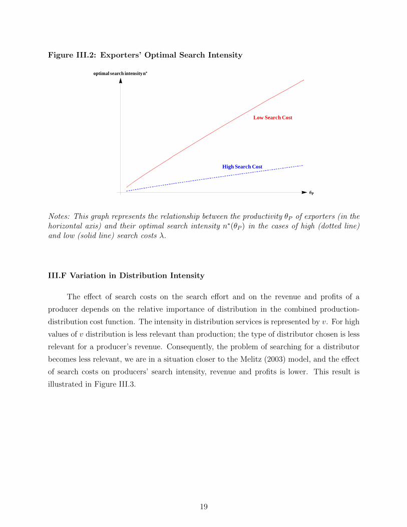
Figure III.2: Exporters’ Optimal Search Intensity

qP

optimal search intensityn*

High Search Cost

Low Search Cost

Notes: This graph represents the relationship between the productivity θP of exporters (in thehorizontal axis) and their optimal search intensity n∗(θP ) in the cases of high (dotted line)and low (solid line) search costs λ.

III.F Variation in Distribution Intensity

The effect of search costs on the search effort and on the revenue and profits of a

producer depends on the relative importance of distribution in the combined production-

distribution cost function. The intensity in distribution services is represented by v. For high

values of v distribution is less relevant than production; the type of distributor chosen is less

relevant for a producer’s revenue. Consequently, the problem of searching for a distributor

becomes less relevant, we are in a situation closer to the Melitz (2003) model, and the effect

of search costs on producers’ search intensity, revenue and profits is lower. This result is

illustrated in Figure III.3.

19

Figure III.3: The Effect of Search Costs on Producers’ Revenue depends on

Distribution Intensity.

v = 14

dashed line v = 34

solid line

Expected Revenue

Notes: This graph represents the relationship between search costs λ and the expected revenueof a producer of productivity θP (held constant in this graph). The dashed line shows the re-lationship for a product for which distribution is relatively important compared to production.In the solid line, distribution is unimportant, and the negative effect of search costs on theproducer’s revenue is lower. In other words, the dashed line has a steeper slope.

III.G “Firm-Level Gravity”

Trade flows between firms depend on the productivity of exporters and importers,

generating a relationship that resembles the gravity equation for trade between countries. I

term this relationship “firm-level gravity”.

Proposition III. The volume of trade between two firms depends:

i) Positively on the productivity of the exporter and the importer.

ii) Negatively on ad-valorem trade costs.

Proof: By inspection of the revenue function describing the traded value between an export-

ing and an importing firm.23

23The revenue of a producer in Home trading with a distributor in Foreign is the following

RHfPH(θPH , θDF ) = AF

(ε · v

ε · v − 1

)1−ε·v (ε

ε− 1

)−ετ (1−ε)·v

(wHθPH

)(1−ε)·v (wFθDF

)(1−ε)·(1−v)

= Zd·θε·v−1PH ·θε·(1−v)DF

20

In contrast, in models based on Melitz (2003) trade flows depend on the characteristics

(typically productivity) of exporting firms only.

III.H Selection into export markets

The model described earlier in this section does not generate an export productivity

cutoff that explains the selection of highly productive firms into export markets as in Melitz

(2003). The model can be extended to include an additional fixed cost of entry into export

markets (F ) to generate this result. The problem for a producer in Home searching for an

importer to reach final consumers in Foreign becomes:

maxn

∫ ∞0

fnmax(θDF ) · πHfPH(θPH , θDF )dθDF − wH · λ · n− wH · F (3.21)

Firms with productivity below θPH = k · ( F ·λδ−1

(ZHf )δ)

1δ·(ε·v−1) do not export, where δ =

γγ−ε·(1−v)

.

21

IV. Exporter-Importer Matches and Trade

Liberalization: the U.S. - Colombia Free Trade

Agreement

The U.S.-Colombia FTA provides an ideal quasinatural experiment to test the theory

of exporter-importer sorting described by the model. The model predicts that by making

the Colombian market more profitable. U.S. exporters find it optimal to incur in larger

search costs in order to find more productive importing partners in Colombia. This reorga-

nization of exporter-importer matches is a novel dimension on the response of firms to trade

liberalization.

The tariff cuts favoring U.S. exporters to Colombia were large and there was substantial

variation across industries. I design an empirical strategy taking advantage of this cross-

industry variation.

The first subsection discusses the theory. Subsection IV.B provides background on

the FTA, and shows that the liberalization led to an increase in U.S. exports to Colombia.

Subsection IV.C discusses the matched exporter-importer data on U.S exporting firms and

Colombian importing firms. The core of the analysis in subsection IV.D links the liberaliza-

tion to the reorganization of exporter-importer matches, in consonance with the mechanisms

in the model.

IV.A The Effect of Trade Liberalization in the Theory

The decline in trade costs (tariffs) faced by U.S. exporters is akin to an exogenous

increase in demand and profitability of the Colombian market in the liberalized industries.

The higher profitability of the export market will lead the U.S. exporters to find it optimally

to incur a larger search effort in order to find a more productive Colombian partner. In other

words, while the marginal cost of search remains constant, its marginal benefit increases.

Finding a more productive importer is more valuable in a more profitable market. The

liberalization makes paying a higher fixed cost (search cost) worth it. Essentially, recall that

the fixed cost of exporting (search cost) is endogenous and optimized by each firm, differently

than in standard heterogeneous-firms trade models.

This partial equilibrium argument is accompanied by general equilibrium results. The

change in the exogenous trade cost parameter leads to an increase in the mass of exporters

22

in the U.S. and the mass of importers in Colombia. The test described below focuses only

on the reorganization of exporter-importer matches.

IV.B The U.S. - Colombia Free Trade Agreement

This section briefly describes the trade agreement and shows it led to an increment

in U.S. exports to Colombia. The free trade agreement signed by the U.S. and Colombia

reduced tariffs starting on May 15th 2012. U.S. exporters to Colombia faced large tariff cuts

in many industries. Most of these were effective immediately and reduced tariffs to zero.

Due to the short span of the post-liberalization period, I focus on these industries in the

empirical design described in section IV.D. These tariff cuts concern a large number of U.S.

firms that export to Colombia, as well as a large number of Colombian importers from the

U.S.

The following figure (IV.1) illustrates the density of the tariff cuts faced by U.S. ex-

porters. Descriptive statistics on these tariffs faced by U.S. exporters in Colombia before and

after the agreement are reported in table IV.1. A first essential observation is that initial

pre-FTA tariffs were large in many industries, and the reduction was also large as many of

these were fully eliminated. A second important point is that there was substantial variation

across industries, as shown in the figure.

The trade data show an increase in U.S. exports to Colombia immediately after the

agreement. A first observation, shown in figure IV.2, is that the ratio of U.S. exports to

Colombia over U.S. exports to other South American markets that did not implement this

tariff cuts rose substantially. While, this pattern is evident at first sight, the figure illustrates

a change in the slope of a line fitted to the trade data before and after the agreement.

23

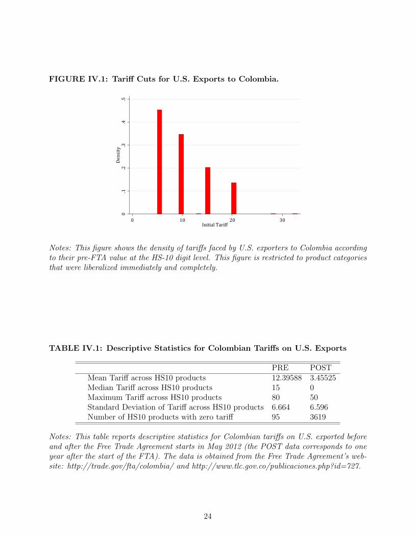
FIGURE IV.1: Tariff Cuts for U.S. Exports to Colombia.

0.1

.2.3

.4.5

Density

0 10 20 30InitialTariff

Notes: This figure shows the density of tariffs faced by U.S. exporters to Colombia accordingto their pre-FTA value at the HS-10 digit level. This figure is restricted to product categoriesthat were liberalized immediately and completely.

TABLE IV.1: Descriptive Statistics for Colombian Tariffs on U.S. Exports

PRE POSTMean Tariff across HS10 products 12.39588 3.45525Median Tariff across HS10 products 15 0Maximum Tariff across HS10 products 80 50Standard Deviation of Tariff across HS10 products 6.664 6.596Number of HS10 products with zero tariff 95 3619

Notes: This table reports descriptive statistics for Colombian tariffs on U.S. exported beforeand after the Free Trade Agreement starts in May 2012 (the POST data corresponds to oneyear after the start of the FTA). The data is obtained from the Free Trade Agreement’s web-site: http://trade.gov/fta/colombia/ and http://www.tlc.gov.co/publicaciones.php?id=727.

24

FIGURE IV.2: The Effect of the FTA on U.S. Exports to Colombia..

.06

.08

.1.1

2.1

4E

xpor

ts to

Col

ombi

a / E

xpor

ts to

Sou

th A

mer

ica

2006m1 2008m1 2010m1 2012m1 2014m1Date

Exports to Colombia/Exports to South America Fitted preFTAFitted postFTA

U.S. Exports to Colombia over U.S. Exports to South America

Notes: This figure shows the evolution of U.S. exports to Colombia as a fraction of U.S. ex-ports to South America at a monthly frequency during January 2006- May 2014 (blue dashedline). The green sold lines correspond to the fitted linear prediction estimated separatelybefore May 2012 and after May 2012. Data is obtained from the U.S. Census Bureau.

To delve deeper into this relationship and establish the causality of the impact of the

FTA on U.S. exports, I use product-level trade data to compare the evolution of U.S. exports

in liberalized and non-liberalized sectors. I show that the Free Trade Agreement increased

exports from the U.S. to Colombia following a triple difference in differences empirical design.

I compare U.S. exports in liberalized industries to non-liberalized industries (first difference)

before and after the agreement (second difference) to Colombia and to other South American

markets (third difference). Specifically, I estimate the following gravity equation for U.S.

exports to Colombia and every other South American country. I construct a categorical

indicator for liberalized industries which I compare to non-liberalized industries. I define

two time periods: pre-agreement (2011) and post-agreement (2013).

log(Exports)cit = β1 · POSTt · libi · Colombiac + β2 · POSTt · libi+

β3 · POSTt · Colombiac + β4 · libi · Colombiac + εcit (4.1)

In this equation, each observation is a product (i) - destination (c) - year (t) com-

25

bination. Products are defined at the HS-6 digit level. While the U.S. export data is

disaggregated upto the HS-10 level, it can only be matched to the Colombian tariffs at the

internationally-standarized HS-6 level. Robust standard errors are clustered by industry,

destination and period using multiway clustering. The data on U.S. exports is obtained

from the U.S. Census Bureau’s “U.S. Exports of Merchandise”.

Table IV.2 reports the results for equation 1. The coefficient of interest on the triple

interaction is positive and economically and statistically significant. It can be interpreted as

an increase in U.S. exports in liberalized industries compared to non-liberalized industries

in Colombia compared to similar South American markets.

TABLE IV.2: The Effect of the FTA on U.S. Exports to Colombia.

Dependent Variable: (log) Value of U.S. Exports by Industry and Country

Postt · libi · Colombiac 0.1332***

0.0175

Postt · Colombiac 0.0174

0.0334

libi · Colombiac 0.0089

0.1020

Postt · libi -0.0115

0.0181

Country F.E. Yes

HS-6 Product F.E. Yes

Time period F.E. Yes

Observations 48039

Notes: This table reports the results of the estimation of equation 4.1. Destination countriesare Colombia, Argentina, Bolivia, Brazil, Chile, Ecuador, Paraguay, Peru, Uruguay andVenezuela. Data is obtained from the U.S. Census Bureau’s “U.S. Exports of Merchandise”which reports U.S. exports disaggregated at the country - HS10 product level. Standard errorsare reported under the estimated coefficients. ***. ** and * denote significance at the 1%,5% and 10% confidence levels.

26

TABLE IV.3: Descriptive Statistics for U.S. Exporters to Colombia

Exporters trading with single partner in PRE and POST 5070In immediately liberalized industries 3565Share switching trading partner 25%Mean Value Exported - PRE (USD) 780 000Mean Value Exported - POST (USD) 948 000

Notes: This table reports descriptive statistics for U.S. exporters to Colombia before andafter the Free Trade Agreement starts in May 2012 (PRE corresponds to 2011/5 to 2012/6and POST to 2013/5 to 2014/6). The first row reports the number of U.S. firms exportingto Colombia in both periods, trading with a single partner in both. The second row reportsthe share of those firms in industries liberalized immediately and completely, which are theones I consider in the analysis. The third column shows the share of those firms switchingpartners between both periods. The last two rows show the mean value exported by these U.S.exporters in each period.

IV.C Data on U.S. Exporters and Colombian Importers

I use the information on import transactions collected by Colombian customs described

in section II.A. These records contain the name of the Colombian importer and the US ex-

porter in each international transaction. The data includes the name, address, city and

telephone number or email address of the US exporters. Since I will be interested in iden-

tifying firms rather than plants, I use the names of these U.S. firms but not their address

to define a firm. On the importing side, I observe the tax ID number of the Colombian

importers, which define a Colombian firm. Table IV.3 presents descriptive statistics on U.S.

exporters to Colombia. Additionally I use balance sheet data on these Colombian importers

to observe their revenue (size) and a measure of their productivity. This data was introduced

in section II.

IV.D The Free Trade Agreement and Exporter-Importer Matches.

I investigate the effect of the trade liberalization on the reorganization of U.S. exporter -

Colombian importer relationships in several steps. First, I show that tariff concessions made

by Colombia to U.S. exporters raised the sales of these exporters in this market. Second, I

find that U.S. exporters respond to tariff cuts by switching their importing partners. Finally,

I show that I show that U.S. exporters that switched importing partners in response to the

tariff cuts chose larger and more productive importing partners.

27

IV.D.1 Tariff Cuts lead to an Increase in the Intensive Margin of Exports.

First I show that tariff cuts in favor of U.S. exporters to Colombia led to an increase in

the value exported by these U.S. firms (i.e. an increase in the intensive margin of exports).

I follow a difference in differences approach, comparing the exports of U.S. firms to

Colombia before and after the agreement and across industries facing different degrees of

liberalization.

I measure the exposure of U.S. exporters to trade liberalization computing the tariff

cut relevant to each exporting firm. I restrict the analysis to firms in sectors liberalized

immediately and completely, which represent the large majority of U.S. exports to Colombia.

The tariff associated to each firm is computed as a weighted average of the tariff of each

of the firm’s products, using product shares in the pre-agreement period as weights. In the

expression below, e indexes U.S. exporters, p indexes HS-6 products. ∆Tariffp stands for

the change in ad-valorem tariffs for product p exported from the U.S. to Colombia and vPREep

is the value exported by exporter e of product p during June 2011 - May 2012 (before the

FTA).24

∆Tariffe =

∑p v

PREep ·∆Tariffp∑

p vPREep

(4.2)

I estimate the following equation, with the change in (log) exports of exporting firm

e as the dependent variable. The independent variable of interest is the change in tariffs

associated to that firm. I define the pre-liberalization period as June 2011-May 2012 and

the post-liberalization period as June 2013 - May 2014.

∆Exportse = β ·∆Tariffe + εe (4.3)

I include industry-level fixed effects at the HS-2 digit level. This means I am comparing

different industries within sectors; for instance, manufacturers of photographic cameras to

manufacturers of video recorders, rather than to producers of pharmaceuticals. I cluster

standard errors according to the tariff category associated to each firm.

I find that U.S. exporters facing larger tariff cuts did increase their exports to Colombia

by more. A one standard deviation larger tariff reduction is associated with a 0.14 standard

deviations larger revenue. The results are reported in table IV.4. Descriptive statistics are

found in the appendix.

24I obtain the tariff data directly from the customs records of Colombias imports. These tariffs are notyet available in the World Banks TRAINS dataset. They are available in the FTA website of the Office ofthe U.S. Trade Representative but are reported in the Colombian classification of 2004, which is difficultto map into more recent HS codes. In the customs data, transactions report the ad-valorem tariff paid. Iaverage these by six digit H.S. code for U.S. exports.

28

Table IV.4: Tariff Cuts lead to an Increase in the Intensive Margin of Exports.

Dependent Variable: ∆(log)Exportse

(1) (2)

∆Tariffe -0.192*** -0.140***

0.062 0.048

(log)Exportse,t−1 -0.435***

0.024

Industry Fixed Effects Yes Yes

Observations 3565 3565

Notes: This table shows the results of the estimation of equation 4.3. All columns includeindustry fixed effects at the HS-2 digit level. All variables are standardized. Standard errorsare reported under the estimated coefficients. Errors are clustered by sector at the HS-2 digitlevel. ***. ** and * denote significance at the 1%, 5% and 10% confidence levels.

IV.D.2 Tariff Cuts lead to Switching Importing Partners.

Next, I ask whether firms facing larger tariff concessions where more likely to switch

their import partners. I focus on firms which exported to Colombia both before and after

the agreement. I restrict the sample to firms with a single partner before and after the

liberalization. I estimate the following equation. The dependent variable Switche takes a

value of one for exporters that switch importers between June 2011 - May 2012 (the initial

interval) and June 2013 - May 2014 (the final interval). The independent variables are again

the change in tariffs associated to each firm, computed as indicated in equation 4.2. As

before, I include HS 2-digit level industry fixed effects to compare once more across similar

industries. Since I include these fixed effects I estimate a linear regression model rather than

of a probit model, to avoid the incidental parameters problem.

Switche = β ·∆Tariffe + εe (4.4)

I find that firms in industries facing larger tariff cuts were more likely to switch to a new

trading partner, as shown in table IV.5. A one standard deviation larger tariff reduction

is associated with a 0.072 standard deviations higher probability of switching importing

partners. The results support the idea that firms have incentives to switch to trading with

more productive importing partners due to the increased profitability in an export market

that results from a liberalization. This idea is explored further in the next subsection.

29

Table IV.5: Tariff Cuts lead to Switching Importing Partners.

Dependent Variable: Switche

(1) (2)

∆Tariffe -0.105** -0.072*

0.045 0.040

(log)Exportse,t−1 -0.279***

0.017

Industry Fixed Effects Yes Yes

Observations 3565 3565

Notes: This table shows the results of the estimation of equation 4.3. All columns includeindustry fixed effects at the HS-2 digit level. All variables are standardized. Standard errorsare reported under the estimated coefficients. Errors are clustered by sector at the HS-2 digitlevel. ***. ** and * denote significance at the 1%, 5% and 10% confidence levels.

IV.D.3 Exporters that Switch their Importing Partner in Response to the

Tariff Cuts Switch to More Productive Importers.

The next question is whether U.S. exporters respond to tariff cuts switching to more

productive importing partners, as the model suggests. Answering this question requires

information on the Colombian importing firms. For this purpose I use the balance sheet

data on Colombian importers based on which I calculate a measure of the productivity of

these importers, as I did in section II.

Once again, I rely on the variation across industries in the extent of tariff cuts. I

estimate the following equation including only the subset of U.S. exporters that switch to a

new partner during the liberalization. The dependent variable ∆Θei is the percentage change

in the productivity between the importing firm (i) trading with a given U.S. exporter (e)

before and after the liberalization. The productivity of the initial and final importing partner

is measured before the agreement in both cases, to prevent the concern that the productivity

of the post-agreement importing partner is influenced directly by the tariff change. The

independent variable is the exporter’s exposure to the trade liberalization, captured by the

tariff cuts relevant to each exporter.

∆Θei = β · Tariffe + εe (4.5)

The number of observatios used for the estimation of equation 4.5 is small because it

30

only includes U.S. exporters i) with a single importing partner before and after the FTA

ii) that switched to a different importing partner during the FTA and iii) exporters trading

with Colombian partners included in the balance sheet data.

I compute the productivity of each Colombian importer as the residual of a regression

of revenue on labor cost and industry fixed effects.25 I include in the estimation of equation

4.5 fixed effects for the industry of the importing firm, at the same level of aggregation

(3-digit ISIC codes) than those used when calculating the productivity of these importing

firms.

The results are reported in table IV.6. Exporters that switch importing partners in

response to the tariff cuts choose more productive importing partners. The estimated co-

efficient indicates that a one standard deviation larger tariff reduction is associated with

0.2 standard deviations higher productivity of the importer. The estimated coefficient is

robust to including the productivity of the exporter’s pre-liberalization importing partner

(Θei,PRE)(column 2) and the pre-liberalization exports of the exporter (column 3).

Table IV.6: Exporters that Switch their Importing Partner in Response to the

Tariff Cuts Switch to More Productive Importers.

Dependent Variable: ∆Θei

(1) (2) (3)

∆Tariffe -0.194* -0.205* -0.203*

0.105 0.114 0.118

Θei,PRE -0.165 -0.171

0.213 0.214

(log)Exportse,t−1 -0.107

0.109

Industry Fixed Effects Yes Yes Yes

Observations 248 248 248

Notes: This table shows the results of the estimation of equation 4.3. All columns includeindustry fixed effects at the ISIC-3 digit level which is the same level used when computingthe productivity of Colombian importers. All variables are standardized. Standard errors arereported under the estimated coefficients. Errors are clustered by sector at the industry level.***. ** and * denote significance at the 1%, 5% and 10% confidence levels.

25Using balance sheet data on Colombian firms I estimate a proxy for productivity as the residual oflog(sales)i = β · log(labor costs)i + φp + εi, where i indexes firms and φp stands for industry (ISIC-3 digit)fixed effects.

31

To summarize, bringing together the findings of subsections IV.D.1, IV.D.2, and IV.D.3,

these results indicate that tariff reductions to U.S. exporters lead them to increase their

export sales, to switch importing partners, and to switch to more productive importing

partners. This pattern is consistent with the theoretical model developed in this paper and

portraits a new mechanism of adjustment of firms to trade liberalization, which highlights

the importance of understanding exporter-importer relationships.

32

V. Conclusions

This paper has studied the interaction between exporting and importing firms, in

the context of international trade based on increasing returns to scale with heterogeneous

exporters and heterogeneous importers. Analyzing jointly the behavior of exporting and

importing firms requires taking into account the selection of these firms into trading pairs.

The paper proposes a simple model in which exporters search for importing firms, with whom

they need to partner to reach final consumers abroad. The sorting of exporters and importers

into trading pairs varies across destinations and across sectors, and has an influence on the

pattern of trade. This represents a departure from existing models of international trade in

which entry into export markets is a black box and the role of importing firms is ignored.

This paper has also provided empirical evidence in support of this theory. In the cross-

section, I establish three new observations using matched exporter-importer data: i) most

exporters trade with a single importer, ii) there is positive assortative matching between

exporters and importers in terms of their productivity, and iii) the value traded is posi-

tively correlated with the productivity of both exporters and importers. Then, using the

Colombia-US Free Trade Agreement as an exogenous shock I provide the first evidence on

the reallocation of exporter-importer matches in response to trade liberalization. As pre-

dicted by the model, U.S. exporters facing larger tariff cuts in the Colombian market adjust

by switching to more productive Colombian importers, which leads to an increase in their

exports in addition to the direct effect of tariff cuts on the intensive margin.

It has been recently stressed that distribution networks or marketing channels could

be important for understanding trade flows. Within the literature on heterogeneous firms

in international trade, a recent survey by Redding (2011) suggests that an “area for further

work is the microeconomic modeling of the trade costs that induce firm selection into export

markets, including the role of wholesale and retail distribution networks.” This paper moves

in that direction by incorporating importing firms into the canonical heterogeneous-firms

trade model.

This paper has stepped away from the typical assumption of frictionless international

markets. In this model, finding partners in foreign markets is costly. This is an old idea,

yet an underexplored one. In this regard, a set of general questions for further research is

the following. Is the relatively high volume of trade experienced in the recent decades (the

so-called second wave of globalization) a consequence of lower transport costs and tariffs or

33

a product of the increased access to information? Second, in their efforts to promote exports

governments frequently subsidize information acquisition. Is this a reasonable policy?

Much is left for future research. One task left pending is to study bargaining in a context

where a set of heterogeneous exporters are confronted to a set of heterogeneous importers.

For instance, one could ask whether it is good or bad news when a small exporter - let’s

say a coffee farmer in a developing country - signs a contract with a very large wholesaler

abroad (rather than with a smaller importer)? More generally, how are the gains from trade

split between exporting and importing countries?

To conclude, one can use this model as a starting point to study other features of trade

contracts. Exporting and importing firms in this model have to set prices and quantities, but

trade contracts in practice are probably more complex. One can study other characteristics of

these contracts, such as their duration, the invoice currency, vertical restraints, and financing

terms, among others.

34

VII. References

AHN, J., KHANDELWAL, A. AND S. WEI (2011): “The role of intermediaries in facilitat-

ing trade,” Journal of International Economics, 84(1), 73-85.

ALLEN, T. (2014): “Information Frictions in Trade,” Econometrica 82(6): 2041-2083.

ANDERSON, J., AND E. VAN WINCOOP (2004): “Trade costs,” Journal of Economic

Literature, 42(3), 691-751.

ANTRAS, P. AND A. COSTINOT (2011): “Intermediated Trade,’ ’Quarterly Journal of

Economics, 126, 1319-1374.

ARKOLAKIS, C. (2010): “Market Penetration Costs and the New Consumers Margin in

International Trade,” Journal of Political Economy, 118 (6), 1151-1199.

BERGER, D., FAUST, J., ROGERS, J., AND STEVERSON, K. (2012): “Border Prices

and Retail Prices,” Journal of International Economics, 88, 62-73.

BERNARD, A., AND DHINGRA, S. (2015): “Contracting and the Division of the Gains

from Trade,” Working Paper.

BERNARD, A., AND JENSEN, B. (1995): “Exporters, Jobs, and Wages in U.S. Manufac-

turing: 1976-1987,” Brookings Papers on Economic Activity. Microeconomics, Vol. 1995:

67-119

BERNARD, A., JENSEN, B., REDDING, S., AND SCHOTT, P., (2007): “Firms in Inter-

national Trade,” Journal of Economic Perspectives. 21(3): 105-30.

BERNARD, A., B. JENSEN, S. REDDING AND P. SCHOTT. (2012): “The Empirics of

Firm Heterogeneity and International Trade,” Annual Review of Economics, Annual Re-

views, 4(1): 283-313, 07.

BERNARD, A., M. GRAZZI, AND C. TOMASI. (2011): “Intermediaries in International

Trade: Direct versus Indirect Modes of Export,’ ’Working paper.

BERNARD, A., A. MOXNES, AND K. ULLTVEIT-MOE. (2014): “Two-Sided Heterogene-

ity and Trade,” Working paper.

BLUM, B., S. CLARO, AND I. HORSTMANN (2010): “Facts and figures on intermediated

trade,” The American Economic Review Papers & Proceedings, 100 (2), 419 - 423.

BLUM, B., S. CLARO, AND I.HORSTMANN (2012): “Intermediation and the nature of

trade costs,” Working paper.

BUSTOS, P. (2011):“Trade Liberalization, Exports, and Technology Upgrading:Evidence on

the Impact of MERCOSUR on Argentinian Firms,” American Economic Review 101:304-

340.

35

CAMERON, C., J. GELBACH, AND D. MILLER (2011):“Robust Inference with Multi-way

Clustering,” Journal of Business and Economic Statistics, 29 (2), 238-249.

CARBALLO, J., G. OTTAVIANO, AND C. VOLPE-MARTINCUS (2013): “The buyer

margins of firms’ exports,” Working Paper.

CHANEY, T. (2011a):“The gravity equation in international trade: An explanation,” Work-

ing paper.

CHANEY, T. (2011b):“The network structure of international trade,” American Economic

Review 104(11): 3600-34.

EATON, J. AND S. KORTUM (2002):“Technology, geography, and trade,” Econometrica,

70(5),1741-1779.

EATON, J., M. ESLAVA, C. KRIZAN, M.KUGLER, AND J.TYBOUT (2011):“A search

and learning model of export dynamics,” Working paper.

FELBERMAYR, B. AND JUNG, B. (2011): “Home Market Effects and the Single-Sector

Melitz Model,” Working Paper.

GLEJSER, H., JACQUEMIN, A., PETIT, J., (1980): “Exports in an Imperfect Competition

Framework: An Analysis of 1,446 Exporters,” The Quarterly Journal of Economics, Vol. 94,

No. 3 (May, 1980), pp. 507-524

GROSSMAN, G., AND MAGGI, G., (2000): “Diversity and Trade”, American Economic

Review, 90(5), 1255-1275.

HELPMAN, E., MELITZ, M., AND RUBINSTEIN, Y., (2008): “Estimating Trade Flows:

Trading Partners and Trading Volumes, Quarterly Journal of Economics, 123(2), 441-487.

KAMAL, F. AND SUNDARAM, A. (2014): “Buyer-Seller Relationships in International

Trade: Do Your Neighbors Matter?,” Working Paper.

KNELLER, R., AND M.PISU (2011): “Barriers to Exporting: What are they and who do

they matter to?,” The World Economy, 34(6), 893-930.

KRAMARZ, F., MARTIN, J., AND MEJEAN, I. (2015): “Volatility in the Small and in the

Large: Diversification in Trade Networks,” Working Paper.

KREMER, M. AND MASKIN, E. (2006): “Globalization and Inequality,” Working Paper.

KRUGMAN, P., (1979):“Increasing returns, monopolistic competition, and international

trade,” Journal of international Economics 9(4) : 469-479.

KRUGMAN, P., (1980):“Scale economies, product differentiation, and the pattern of trade,”

The American Economic Review 70(5): 950-959.

MACCHIAVELLO, R. (2010): “Development Uncorked: Reputation Acquisition in the New

Market for Chilean Wines in the UK,” Working Paper.

MACCHIAVELLO, R. AND MORJARIA, A. (2015): “The Value of Relationships: Evi-

dence from a Supply Shock to Kenyan Rose Exports,” Working Paper.

36

MELITZ, M., AND OTTAVIANO, G., (2008): “Market Size, Trade and Productivity,” Re-

view of Economic Studies, 75(1), 295-316.

MILGROM, P. AND ROBERTS, J., (1990): “The Economics of Modern Manufacturing:

Technology, Strategy and Organization,” American Economic Review, 80(3), 511-528.

MONARCH, R. (2015): “It’s Not You, It’s Me: Breakups in U.S.-China Trade Relation-

ships,” Working Paper.

OHLIN, B., (1933): “Interregional and international trade,” (Harvard University Press).

RAUCH, J. (1996): “Trade and Search: Social Capital, Sogo Shosha, and Spillovers,’ ’Work-

ing paper.

RAUCH, J. (1999): “Networks versus markets in international trade,” Journal of Interna-

tional Economics, 48(1), 7-35.

REDDING, S., (2011): “Theories of Heterogeneous Firms and Trade,” Annual Review of

Economics, 3, 77-105.

SUGITA, Y., KENSUKE, T., AND SEIRA, E. (2015): “Assortative Matching of Exporters

and Importers,” Working Paper.

STIGLER, G. (1961): “The Economics of Information,” The Journal of Political Economy,

69(3), 213-225.

TINBERGEN, J. (1962): “Shaping the World Economy: Suggestions for an International

Economic Policy, New York.

TIROLE, J, (1988): “The Theory of Industrial Organization, The MIT PRESS.

WOOLDRIDGE, J. (2010): “Econometric Analysis of Cross Section and Panel Data,” MIT

Press, Second Edition.

37

VIII. Empirical Appendix - For Online Publication

VIII.A Descriptive Statistics for Section II

The following table presents descriptive statistics for the dataset used in section II.

These are descriptive statistics for the non-standardized variables. Productivity is shifted to

have a mean zero. Coefficients in tables II.2 and II.3are based on these variables standardized

to have mean 0 and standard deviation 1.

Table VIII.1: Descriptive Statistics for the data on French exporters and

Colombian importers.

Mean Std. Deviation

Traded Value 10.235 2.223

Exporter - Revenue 17.415 2.041

Importer - Revenue 17.564 1.941

Exporter - Revenue minus bilateral trade 17.405 2.057

Importer - Revenue minus bilateral trade 16.899 1.958

Exporter - Estimated Productivity 0 0.642

Importer - Estimated Productivity 0 0.877

VIII.B Descriptive Statistics for Section IV.

The following table presents descriptive statistics for the dataset used in the estima-

tion of equations 4.3, 4.4 and 4.5 in section IV. These are descriptive statistics for the

non-standardized variables. Coefficients in tables IV.4, IV.5, and IV.6, are based on these

variables standardized to have mean 0 and standard deviation 1.

38

Table VIII.1: Descriptive Statistics for Equation 4.3.

Mean Std. Deviation

∆(log)Exportse 0.009 1.807

∆Tariffe -1.391 3.423

(log)Exportse,t−1 10.134 2.130

Table VIII.1: Descriptive Statistics for Equation 4.4.

Mean Std. Deviation

Switche 0.250 0.433

∆Tariffe -1.391 3.423

(log)Exportse,t−1 10.134 2.130

Table VIII.1: Descriptive Statistics for Equation 4.5.

Mean Std. Deviation

∆Θei -2.366 20.740

∆Tariffe -1.298 2.575

Θei,PRE 0.582 1.024

(log)Exportse,t−1 9.387 1.811

39

IX. Theory Appendix - For Online Publication

Subsections IX.A, IX.B and IX.C contain additional theoretical results. Subsections

IX.D show the details of the solution of the partial equilibrium problem of the exporting firm.

Subsection IX.E presents a variation in the case of Nash bargaining between exporters and

importers. Subsection IX.F presents the solution to the general equilibrium model. Finally,

subsection IX.G contains proofs to each proposition.

IX.A Wages and Welfare

Differences in country size lead to differences in wages. As in the two-country Melitz

(2003) model with symmetric trade costs (see Felbermayr and Jung (2011)) it can be shown

that:

Proposition IV. The larger country has a higher wage.

Proof: See subsection IX.G.

This result is equivalent to that in Krugman (1980) with homogeneous firms. Under

costly trade, a wage differential is needed offset the attractiveness of the larger market to

producers in order to keep labor fully employed in both markets.

Welfare is measured by the real wage in each country, Wi = wiPi

. As in the Melitz (2003)

model, under costly trade welfare is higher in the larger country. In this case, this is found

numerically, simulating the model for a wide variety of parameters.

IX.B Gravity in a Many-Country World

In partial equilibrium we can think of a many-country version of the model and derive

a gravity equation that relates the volume of trade between two countries to their income

and trade costs. The aggregate gravity equation derived from this model includes both the

usual trade costs as well as search costs. Recall that Tinbergen’s (1962) explanation for

the role of distance in the inaugural gravity equation was not only an approximation for

transport costs but also a representation of information frictions: “The factor of distance

may also stand for an index of information about export markets”.

Consider an M-country version of the model described earlier. Preferences in each

country are identical, and transport costs and search costs vary across country pairs but are

40

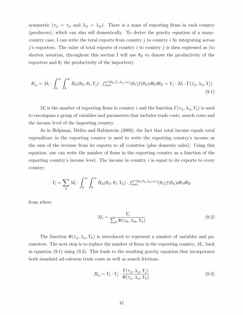
symmetric (τij = τji and λij = λji). There is a mass of exporting firms in each country

(producers), which can also sell domestically. To derive the gravity equation of a many-

country case, I can write the total exports from country j to country i by integrating across

j’s exporters. The value of total exports of country i to country j is then expressed as (to

shorten notation, throughout this section I will use θE to denote the productivity of the

exporters and θI the productivity of the importers):

Rij = Mi ·∫ ∞

0

∫ ∞0

RE(θE, θI , Yj) · fn∗(θE ,Yj ,λij ·wi)

max (θI)f(θE)dθIdθE = Yj ·Mi · Γ(τij, λij, Yj)

(9.1)

Mi is the number of exporting firms in country i and the function Γ(τij, λij, Yj) is used

to encompass a group of variables and parameters that includes trade costs, search costs and

the income level of the importing country.

As in Helpman, Melitz and Rubinstein (2008), the fact that total income equals total

expenditure in the exporting country is used to write the exporting country’s income as

the sum of the revenue from its exports to all countries (plus domestic sales). Using this

equation, one can write the number of firms in the exporting country as a function of the

exporting country’s income level. The income in country i is equal to its exports to every

country:

Yi =∑h

Mi ·∫ ∞

0

∫ ∞0

RE(θE, θI , Yh) · fn∗(θE ,Yh,λih·wi)

max (θI)f(θE)dθIdθE

from where

Mi =Yi∑

h Φ(τih, λih, Yh)(9.2)

The function Φ(τij, λij, Yh) is introduced to represent a number of variables and pa-

rameters. The next step is to replace the number of firms in the exporting country, Mi, back

in equation (9.1) using (9.2). This leads to the resulting gravity equation that incorporates

both standard ad-valorem trade costs as well as search frictions.

Rij = Yi · Yj ·Γ(τij, λij, Yj)

Φ(τij, λij, Yh)(9.3)

41

IX.C Final Prices and Border Prices

The model features a final price paid by consumers in the destination market, pf ,

and the price of the transaction at the border (the “border price”, “international price” or

“wholesale price”, pw) paid by the importer to the exporter. The ratio between these prices

is typically large and has been studied by Berger et al (2012) and others.26

Consider again the many country world of subsection III.J. In the model, this price

ratio pf/pw varies across exporting firms and destinations. It also depends on industry

characteristics.

Consider the variation in the expected price ratio for a given exporting firm across

destinations, E[pf/pw|θE]. Large search costs lead exporters to reduce their search intensity.

This results in matches with low-productivity importers (i.e. a higher marginal cost for the

distribution of the products) and the price ratio of border to retail prices pf/pw increases.

Exporting firms that face high entry barriers in the Colombian market (for instance an

exporter from Pakistan to Colombia which will likely face a large search cost parameter) have

a large pf/pw ratio, while firms facing small entry barriers (a small search cost parameter)

have a small pf/pw ratio.

IX.D Solution to the Producer’s Problem

Producers maximize their expected profits choosing an optimal search intensity n.

Consider the case of a producer in Home of productivity θPH searching for a distributor in

Foreign. The maximization problem is the following:

maxn

∫ ∞0

fnmax(θDF )πHfPH(θPH , θDF )dθDF − wH · λ · n

The first term in this equation represents the expected operating profits for the producer

obtained from a trading relationship with a distributor of productivity θDF , given a search

effort n. The integrand is the probability of being matched with a certain distributor times

the operating profits that the producer obtains from the relationship. The second term is

the cost of the search effort.

We can rewrite the maximization problem after replacing these terms as:

26Berger et al (2012) find that for U.S. imports the gap (pf − pw)/pw is on average in the range 50% -70%. Berger et al (2012) measure pf using the BLS’ CPI microdata and pw using the BLS’ IPP microdata.

42

maxn ZHf · θε·v−1

PH ·∫ ∞

0

γ · n · θ−γ−1DF · e−n·θ

−γDF · θε·(1−v)

DF · dθDF − wH · λ · n

To evaluate the integral, define t = n·θ−γDF and integrate in terms of t. The maximization

problem is:

maxn ZHf · θε·v−1

PH ·∫ ∞

0

nb · t−b · e−t · dt− wH · λ · n

Note that ∫ ∞0

nb · t−b · e−t · dt = nb ·∫ ∞

0

t−b · e−t · dt = nb ·R

with R = Γ(1− b) and b = ε·(1−v)γ

.

The maximization problem is then

maxn (ZHf · θε·v−1PH ·R · nb − λwH n)

the solution of which is

n∗(θPH , ZHf , λ) = k ·

(ZHf · θε·v−1

PH

λ · wH

)γ/(γ−ε·(1−v))

,

where k =

(ε·(1−v)·Γ( γ−ε·(1−v)γ )

γ

)γ/(γ−ε·(1−v))

IX.E The Case with Nash-Bargaining between Exporters and Importers

In the model discussed in section III, producers set the wholesale price at which they

sell to distributors. Based on this price, distributors choose the optimal final price. An

alternative way of modeling the interaction between producers and distributors is such that

these firms jointly set the final price and bargain over the surplus generated by the trading

partnership. This case is briefly discussed below. The results described in section III still

hold in this case. In the model below I assume all outside options are zero, so the share of

surplus obtained by exporters is always the same. This is unrealistic, but accounting for the

43

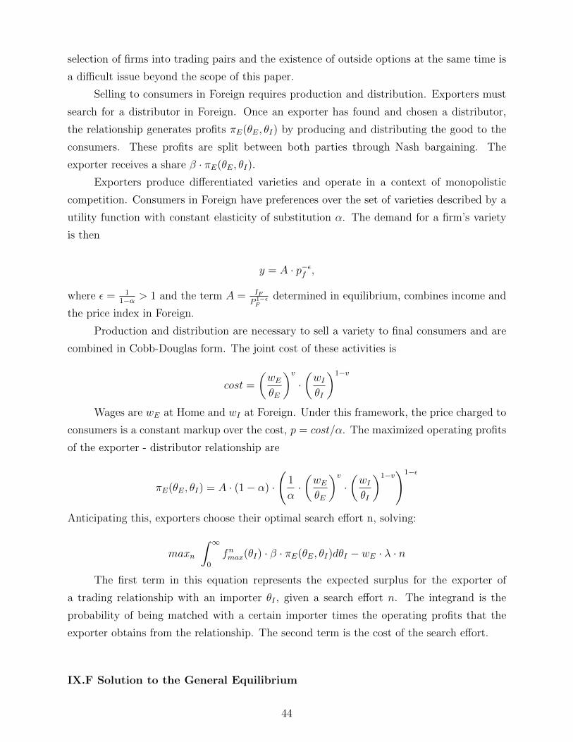
selection of firms into trading pairs and the existence of outside options at the same time is

a difficult issue beyond the scope of this paper.

Selling to consumers in Foreign requires production and distribution. Exporters must

search for a distributor in Foreign. Once an exporter has found and chosen a distributor,

the relationship generates profits πE(θE, θI) by producing and distributing the good to the

consumers. These profits are split between both parties through Nash bargaining. The

exporter receives a share β · πE(θE, θI).

Exporters produce differentiated varieties and operate in a context of monopolistic

competition. Consumers in Foreign have preferences over the set of varieties described by a

utility function with constant elasticity of substitution α. The demand for a firm’s variety

is then

y = A · p−εf ,

where ε = 11−α > 1 and the term A = IF

P 1−εF

determined in equilibrium, combines income and

the price index in Foreign.

Production and distribution are necessary to sell a variety to final consumers and are

combined in Cobb-Douglas form. The joint cost of these activities is

cost =

(wEθE

)v·(wIθI

)1−v

Wages are wE at Home and wI at Foreign. Under this framework, the price charged to

consumers is a constant markup over the cost, p = cost/α. The maximized operating profits

of the exporter - distributor relationship are

πE(θE, θI) = A · (1− α) ·

(1

α·(wEθE

)v·(wIθI

)1−v)1−ε

Anticipating this, exporters choose their optimal search effort n, solving:

maxn

∫ ∞0

fnmax(θI) · β · πE(θE, θI)dθI − wE · λ · n

The first term in this equation represents the expected surplus for the exporter of

a trading relationship with an importer θI , given a search effort n. The integrand is the

probability of being matched with a certain importer times the operating profits that the

exporter obtains from the relationship. The second term is the cost of the search effort.

IX.F Solution to the General Equilibrium

44

Consider first the zero profit conditions for producers in Home. In what follows θE

represents the productivity of an exporter (producer) and θI the productivity of an importer

(distributor). For notational simplicity I omit some of the subindices present in the main

text.

∫ ∞0

∫ ∞0

(ZHHθε v−1

E θε (1−v)I − λwHn∗(θE, ZHH , λwH)

)fn

∗(θE ,ZHH ,λwH)

max (θI)f(θE) dθI dθE+∫ ∞0

∫ ∞0

(ZHF · θε v−1

E θε (1−v)I − λwHn∗(θE, ZHF , λwH)

)fn

∗(θE ,ZHF ,λwH)

max (θI) f(θE) dθI dθE

= wH FH (9.4)

and for producers in Foreign:

∫ ∞0

∫ ∞0

(ZFF θε v−1

E · θε (1−v)I − λwF n∗(θE, ZFF , λwF )

)fn

∗(θE ,ZFF ,λwF )

max (θI) f(θE) dθI dθE+∫ ∞0

∫ ∞0

(ZFH θε v−1

E · θε (1−v)I − λwF · n∗(θE, ZFH , λwF )

)· fn∗(θE ,Z

FH ,λwF )max (θI) f(θE) dθI dθE

= wF FF (9.5)

where

ZHH =wH · LH ·

(ε·vε·v−1

)−ε·v · ( εε−1

)−ε · ( εε−1

)· w1−ε·v

H · w−ε·(1−v)H

P 1−εH

ZHF =wF · LF · τ 1−εv( ε·v

ε·v−1

)−ε·v · ( εε−1

)−ε · ( εε−1

)· w1−ε·v

H · w−ε·(1−v)F

P 1−εF

ZFH =wH · LH · τ 1−εv( ε·v

ε·v−1

)−ε·v · ( εε−1

)−ε · ( εε−1

)· w1−ε·v

F · w−ε·(1−v)H

P 1−εH

ZFF =wF · LF ·

(ε·vε·v−1

)−ε·v · ( εε−1

)−ε · ( εε−1

)· w1−ε·v

F · w−ε·(1−v)F

P 1−εF

After some algebra, the zero profit conditions for producers in Home and Foreign can

be written as:

45

ZHHδ ·∫ ∞

0

∫ ∞0

S · θδ·(ε·v−1)E · λδ−1 · f(θE) · dθE+

ZHF δ ·∫ ∞

0

∫ ∞0

S · θδ·(ε·v−1)E · λδ−1 · f(θE) · dθE = wH · FH (9.6)

and for producers in Foreign:

ZFF δ ·∫ ∞

0

∫ ∞0

S · θδ·(ε·v−1)E · λδ−1 · f(θE) · dθE+

ZFHδ ·∫ ∞

0

∫ ∞0

S · θδ·(ε·v−1)E · λδ−1 · f(θE) · dθE = wF · FF (9.7)

This is a linear system for Pδ·(ε−1)H and P

δ·(ε−1)F . We obtain expressions for these price

indices as functions of the wages. The terms S and δ group a number of parameters.

Next consider the equations for the price indices in Home and Foreign.

In Home:

P 1−εH = MH ·K ·wvH ·w1−v

H ·∫ ∞

0

∫ ∞0

θ(ε−1)·vE ·θ(ε−1)·(1−v)

I ·fn∗(θE ,ZHH ,λ·wH)

max (θI)·f(θE)·dθI ·dθE+

MF ·K · wvF · w1−vH ·

∫ ∞0

∫ ∞0

θ(ε−1)·vE · θ(ε−1)·(1−v)

I · fn∗(θE ,ZFH ,λ·wF )

max (θI) · f(θE) · dθI · dθE

(9.8)

In Foreign:

P 1−εF = MH ·K ·wvH ·w1−v

F ·∫ ∞

0

∫ ∞0

θ(ε−1)·vE ·θ(ε−1)·(1−v)

I ·fn∗(θE ,ZHF ,λ·wH)

max (θI)·f(θE)·dθI ·dθE+

MF ·K · wvF · w1−vF ·

∫ ∞0

∫ ∞0

θ(ε−1)·vE · θ(ε−1)·(1−v)

I · fn∗(θE ,ZFF ,λ·wF )

max (θI) · f(θE) · dθI · dθE,

(9.9)

where I have used K = εε−1·(

εvεv−1

)v.

The equations for the price index in Home and Foreign are a linear system in terms of

the mass of producers in Home and Foreign, MH and MF . Given that we can find the price

indices as functions of the wages from the zero profit conditions, we obtain also expressions

for the mass of producers as functions of the wages.Since this is a linear system, this is solved

46

analytically.

Next, we replace these terms in the balanced trade condition, set one wage as the

numeraire and solve for the other one. The balanced trade condition is the following.

MH ·∫ ∞

0

∫ ∞0

ZHF · ε · v · θε·v−1E · θε·(1−v)

I · fn∗(θE ,ZHF ,λ·wH)

max (θI) · f(θE) · dθI · dθE =

MF ·∫ ∞

0

∫ ∞0

ZFH · ε · v · θε·v−1E · θε·(1−v)

I · fn∗(θE ,ZFH ,λ·wF )

max (θI) · f(θE) · dθI · dθE (9.10)

Finally the mass of importers in each country, NH and NF is obtained by replacing the

solution into the zero profit condition of importers. A useful property of the model is that

the mass of importers does not affect the other equilibrium variables.If search were modeled

differently, this would not hold.

The zero profit condition for importers in Home is the following. J denotes the cost of

entry into importing.

∫ ∞0

∫ ∞0

fn∗(θE ,Z

HH ,λ·wH)max (θI)·

1

NH · f(θI)·BHH ·θ(ε−1)·v

E ·θ(ε−1)·(1−v)I ·MH ·f(θE)·f(θI)·dθI ·dθE+∫ ∞

0

∫ ∞0

fn∗(θE ,Z

FH ,λ·wF )max (θI)·

1

NH · f(θI)·BFH ·θ(ε−1)·v

E ·θ(ε−1)·(1−v)I ·MF ·f(θE)·f(θI)·dθI ·dθE = wH ·JH

(9.11)

In Foreign:

∫ ∞0

∫ ∞0

fn∗(θE ,Z

HF ,λ·wH)max (θI)·

1

NF · f(θI)·BHF ·θ(ε−1)·v

E ·θ(ε−1)·(1−v)I ·MH ·f(θE)·f(θI)·dθI ·dθE+∫ ∞

0

∫ ∞0

fn∗(θE ,Z

FF ,λ·wF )max (θI)·

1

NF · f(θI)·BFF ·θ(ε−1)·v

E ·θ(ε−1)·(1−v)I ·MF ·f(θE)·f(θI)·dθI ·dθE = wF ·JF

(9.12)

In these equations,

Bij =wj · Lj ·

(ε·vε·v−1

)1−ε·v ·(

εε−1

)−ε · ( εε−1

)· w1−ε·v

i · w1−ε·(1−v)j

P 1−εj

The mass of importers in each country is obtained from these equations once the other

equilibrium variables have been determined.. This can be done analytically.

This ends the solution to the general equilibrium.

47

IX.G Proofs to Propositions in section III.

Proof to Proposition I.

That more productive search more is seen by inspection of exporters’ optimal search

intensity (3.6). Under the restrictions imposed on the parameters, it is verified that the

derivative of n∗ with respect to θPH is positive.

Proof to Proposition II.

From the expression for an exporter’s optimal search intensity, one can see that the

search cost parameter λ impacts the exporter’s decision both directly and through the price

index. From the solution to the general equilibrium, as described in the previous section,

one can write the price indices as functions of the wages and the search cost parameter.

Under symmetric trade costs (the case in which I focus), the search cost parameter does not

affect the price indices through the wages, only through the direct effect. In this way one

can directly calculate the derivative of the price index to the search cost parameter, which is

then used to calculate the derivative of the exporter’s optimal search intensity with respect

to the search cost parameter.

From the explicit solution for PF and PH it follows that both PH and PF depend on λ

as

P ≈ λ1−δδ(1−ε) ,

where δ = γi/(γi− ε(1− v)). From the expression for n∗ we know that n∗ ≈ (Z/λ)δ. Since Z

depends on λ through the price indices we obtain that n∗ is proportional to 1/λ. Therefore

dn∗/dλ < 0.

Proof to Proposition IV.

I can write the balanced trade condition as a relationship between the relative wage

y = wFwH

and relative country sizes LH/LF as

LHLF

= H(y)

where

H(y) =X(y)(1+δc)/δ

yδc

[1 + yr(τy)p

X(y)

][(τ/y)p + yr

X(y)

]with

X(y) =1− τ δ(y/τ)δε v

1− τ δ(yτ)−δε v,

48

p = v(1− ε) + δc(1− ε v)

and

r = δ[(b− c) + ε(2 v − 1)]− δ(1− ε).

I can prove that the relationship between relative country size and relative wages is

monotonic, that identical countries have identical wages, and that the larger country will

have a higher wage.

To prove this, I show that H(y) is a decreasing function of y. The steps of the proof

are the following:

First, by taking its derivative we prove that X(y) decreases monotonically with y. Next

verify that defining Z ≡ y(r+p)/X(y) and Q ≡ (1 + τ pZ)/(τ p + Z) H(y) can be written as

H(y) =X(y)(1− b

ε)

yδ v(ε−1)Q (9.13)

where we used that1 + δc

δ= 1− b

ε, δc− p = δ v(ε− 1).

Next, verify that Z increases with y, and that Q decreases with y.

Finally we see that the above implies that H(y) decreases with y. Effectively, since

X(y),Q and y are positive and, since 1 − b/ε > 0 the terms in the numerator of (9.13)

decrease with y and the term in the denominator increases with y (because ε − 1 > 0).

Therefore H(y) decreases with y.

49