the maize farmthe maize farm- ---market price … · the maize farmthe maize farm- ---market price...

GRIPS GRIPS GRIPS GRIPS Discussion PaperDiscussion PaperDiscussion PaperDiscussion Paper 10101010----22225555

The Maize FarmThe Maize FarmThe Maize FarmThe Maize Farm----Market Price Spread Market Price Spread Market Price Spread Market Price Spread

in Kenya and Ugandain Kenya and Ugandain Kenya and Ugandain Kenya and Uganda

ByByByBy

Takashi Yamano Takashi Yamano Takashi Yamano Takashi Yamano

and and and and

Ayumi AraiAyumi AraiAyumi AraiAyumi Arai

DecemberDecemberDecemberDecember 2010201020102010

National Graduate Institute for Policy Studies

7-22-1 Roppongi, Minato-ku,

Tokyo, Japan 106-8677

GRIPS Policy Research Center Discussion Paper: 10-25

1

The Maize Farm-Market Price Spread in Kenya and Uganda

Takashi Yamano1 and Ayumi Arai

2

Abstract

In this chapter, we analyze the farm-market price spreads of maize in Kenya and Uganda to

examine how agricultural sectors are integrated with local markets. The farm-market price

spread is calculated by subtracting the farm-gate price from the market price at the nearest

maize market. We find that the farm-market price spread of maize is about 15 and 33 percent

of the market price in Kenya and Uganda, respectively. In both countries, the price spread

increases by 2 percentage points for each additional driving hour away from the nearest maize

market. While the former finding suggests that the overall marketing costs are lower in Kenya

than in Uganda, the latter finding indicates that reductions in transportation costs will increase

the farmer prices of maize in both countries.

Keywords: Price Spread, Market, Maize, Kenya, Uganda

1 Foundation for Advanced Studies on International Development, National Graduate Institute

for Policy Studies, Japan

2 National Graduate Institute for Policy Studies, Japan

Correspondent author, Takashi Yamano, Foundation for Advanced Studies on International

Development, National Graduate Institute for Policy Studies, 7-22-1, Roppongi, Minato-ku,

Tokyo, 106-8677, Japan [email protected]


2

1. Introduction

A well-integrated market system is considered to be necessary not only for the efficient

allocation of productive resources but also for a reduction in price risks by preventing

unnecessary price volatility. In developing countries where local markets are fragmented, a

localized crop scarcity can lead to famine in the area (Ravallion, 1986). The lack of market

integration has been a major concern for countries in Sub-Saharan Africa where domestic

markets are sparsely located due to low population densities and are isolated from international

markets if the countries are landlocked. Indeed, previous studies find that landlocked countries

are vulnerable to domestic production shocks and experience large price volatilities (Byerlee et

al., 2006). Because poor people, including the urban poor, spend a large share of their total

expenditure on food crops, they would benefit from reduced price volatilities due to market

integration. Thus, linkages to marketing centers have been found to contribute to rural

households’ efforts to escape from poverty (Krishana, 2004; Minot, 2007).

To integrate markets and enable the markets, not government agencies, allocate

resources, structural adjustment programs were implemented in the 1980s and 1990s in many

countries in SSA. To examine the impacts of the structural adjustment programs on market

integration, there have been many studies that have tested market integration internationally

and domestically by using time series data. Some studies find improved market integration


3

after the liberalization (Badiane and Shively, 1998), while others find that markets remain

poorly integrated even after the introduction of the structural programs (Lutz et al., 2006;

Negassa et al., 2004; Fafchamps, 2004; Poulton et al., 1998). In Africa, particular, there are

some studies that examined market integration of cereal crops, such as maize (Faminow and

Laubscher, 1991; Campenhout, 2007; Goletti and Babu, 1994; Rashid, 2004). These studies,

however, only examine integration from the perspective of price correlation across markets.

Even if markets are well integrated across space, local farmers would not benefit from market

integration if their market access is poor. Previous studies find that many small-scale farmers

remain at the subsistence level, not selling their crops at markets (Jayne et al., 2006; Barrett,

2008).

To examine how agricultural sectors, consisting of small-scale farmers, are integrated

with local markets, we analyze the farm-market price spreads of maize in Kenya and Uganda.

The farm-market price spread is calculated by subtracting the farm-gate price from the market

price at the nearest maize market. Because we think transportation costs contribute to the

farm-market price spread significantly, we examine the relationship between the farm-market

price spread and the driving time from each sample household to the nearest maize market

where we have monthly maize price data. We are able to measure the driving time from each

sample household to the nearest maize market from having geo-referenced each sample


4

household and the closest major maize markets. By using digitized road maps of Kenya and

Uganda, we identify four road types and assign an average driving speed on each road type. To

measure the farm-market price spread, we compare the average market price in the four month

period following harvest at the nearest market with the farm-gate maize price obtained from

household surveys. In this chapter, we find that the farm-market price spread of maize is about

15 and 33 percent of the market price in Kenya and Uganda, respectively. In both countries, the

price spread increases by 2 percentage points for each additional driving hour away from the

nearest maize market. While the former finding suggests that the overall marketing costs are

lower in Kenya than in Uganda, the latter finding indicates that additional transportation cost

associated with an increase in driving time affects the marketing cost equally between the two

countries.

The chapter is organized as follows. Section 2 describes the maize markets in Kenya and

Uganda. Section 3 explains the market price data and the household panel data used in this

chapter and presents descriptive analyses of the farm-market price spreads. The estimation

models and variables are explained in Section 4, while the estimation and simulation results are

discussed in Section 5. Finally, we discuss policy implications in Section 6.


5

2. Maize Markets in Kenya and Uganda

In 1988, during the structural adjustment period, the Kenyan government liberalized

its maize market by allowing private traders to operate legally, instead of illegally as was the

case before the liberalization, while keeping the National Cereals and Produce Board (NCPB)

active. Before the liberalization, the NCPB was the sole agency who could procure and sell

maize at administratively determined prices. Even after the liberalization, the NCPB continued

to procure and sell maize at administratively determined prices, and to store maize as a

contingency against future shortages. Jayne et al. (2008) find that NCPB activities have

stabilized maize market prices in Kenya and raised average price levels roughly by 20 percent

between 1995 and 2004.

According to Jayne et al. (2006), only 30 percent of their nationwide sample

households in rural Kenya are net sellers of maize, and roughly 50 percent of all the maize sold

is from fewer, than 3 percent of households. Thus, the increased maize price due to the NCPB

activities has benefited a small number of small-scale maize farmers who are net sellers of

maize, as well as large-scale commercial maize farmers. The increased maize price, however,

is like a tax imposed on urban consumers and small-scale maize farmers who are net buyers of

maize. Indeed, these groups have opposed NCPB activities that raise maize prices. Thus, the

Kenyan government faces a classic “food price dilemma,” where it is pressured to keep the


6

maize price high for net maize sellers while it is pressured to do the opposite for urban

consumers and net-maize-buyer farmers.

Regarding trade policy, the Kenyan government imposed various tariffs on maize

imports at border crossings to support domestic maize prices until January 2009.1 However,

because the Kenya-Uganda border is wide and difficult to monitor, informal cross border trade

occurred regularly. According to the Regional Agricultural Trade Intelligence Network

(RATIN)2 which monitors regional agricultural commodity trade flows at selected border

crossings between countries, the average amount of maize export from Uganda to Kenya was

about 160,000 tons in the three-year period of 2005 to 2007 (Benson et al., 2008). As a result,

Kenya imported about 5 percent of its maize consumption from Uganda during this period. It

was argued that the NCPB support price policy encouraged maize imports from Uganda at the

same time that the official trade policy attempted to suppress it.

In Uganda, maize is the third most important staple crop, after plantain and cassava, in

terms of caloric intake and is widely produced nationwide, especially in eastern region toward

1 In 2008, after poor maize harvests and restrictions on maize imports, the maize price increased

dramatically. The food crisis deepened with allegations of corruption over the issuing of import licenses

and a lack of transparency over the sale of subsidized NCPB grain (Ariga et al., 2010). The allegations

have led to the sacking of most of the NCPB Board of Directors and 17 senior managers. In January

2009, responding to the food crisis and allegations, the Kenyan government lifted the import duty on

maize, allowing importers to buy maize from the international market. Note, however, that the analyses

of this chapter use data taken in the period from 2003 to 2007 when the Kenyan government imposed

import duties on maize. 2 RATIN data are available from http://www.ratin.net/.


7

Kenya. Although the Ugandan government currently does not impose export duties on maize

exports to Kenya, informal interviews with Ugandan traders suggest that the Ugandan

government has prohibited maize exports at border controls after major drought seasons in the

country. Like Kenya, Uganda also cannot escape from the food price dilemma.

One way to address the food price dilemma is to reduce the farm-market price spread,

which measures the price gap between the farm-gate price that farmers receive and the market

price that consumers pay. If the farm-market price spread is reduced, maize farmers can receive

a higher farm-gate price, while keeping the market price constant. The farm-market price

spread can be reduced by reducing the transportation and transaction costs of trading maize

through investing in transportation infrastructure and developing competitive market

institutions. In the following sections, therefore, we focus on the farm-market price spread and

examine its determinants.

3. Price Data and Driving Hours

3.1 Market price and household data

The monthly market data used in this chapter come from RATIN. RATIN has monthly

maize market price data from 9 major markets in Kenya, but only four markets (Mombasa,


8

Nairobi, Eldoret, and Kisumu) have relatively adequate monthly data with fewer missing

months than the other five markets. Among the four markets with adequate data, we choose

three markets (i.e., Nairobi, Eldoret, and Kisumu) that are located near our sample households

who live in Central and Western Kenya. In Figure 1, we present the locations of the maize

markets where we have monthly maize price data and the sample households. In Uganda, only

Kampala has adequate monthly price data of maize in the RATIN data set. As a result, we use

the RATIN monthly maize price data from four cities in Kenya and Uganda. As one can see in

the figure, some households in Uganda are located closer to Kisumu than to Kampala. As

mentioned earlier, RATIN data on regional trade indicate significant maize exports from

Uganda to Kenya. Thus, for some maize producers in Uganda, the maize market prices at

Kisumu are more important than the Kampala maize price. Thus, we calculate the driving time

from each household in Uganda to the two maize markets, i.e., Kampala and Kisumu, and

choose the closest maize market for each household. Later in this section, we explain in detail

how we select the nearest market for each household and calculate the driving time.

The household data used in this chapter come from household-level panel surveys in

Kenya and Uganda, collected as part of the Research on Poverty and Environment and

Agricultural Technology (RePEAT) Project. All surveys employ comparable questionnaires

across countries and time. In addition, soil samples were collected from maize fields when the


9

first rounds of the surveys were conducted. The surveys in Kenya were conducted in 2004 and

2007. The first round of the surveys covered 899 randomly selected households located in 100

sub-locations scattered in the central and western regions of Kenya.3 In the second round,

seven sub-locations in Eastern province were dropped because of the scale reduction of the

survey project. Thus, in this chapter, we drop the samples from Eastern province in Kenya for

the analysis below since we apply statistical methods relying on the longitudinal features of the

data. In addition, attrition also reduced the number of households interviewed. As a result, out

of the 777 targeted households, 725 households were revisited for the survey, resulting in an

attrition rate of 6.7 percent.4

The surveys in Uganda cover 94 rural Local Council 1 areas (LC1s) that are located

across most regions in Uganda, except the North where security problems exist.5 From each

rural LC1, ten households are randomly selected, resulting in a total of 940 small farm

households. The second round was conducted in 2005, and 895 households out of the 940

3 These two waves of surveys in Kenya were conducted by Tegemeo Institute, with financial

and technical help from National Graduate Institute for Policy Studies (GRIPS). 4 We estimated the determinants of the attrition from the surveys and found that none of the

independent variables is significant at the 5 percent level. Thus, we think that the attrition

mostly occurred randomly and do not expect serious attrition biases. 5 The surveys in Uganda were conducted jointly by Makerere University, Foundation for

Advanced Studies on International Development (FASID), and National Graduate Institute for

Policy Studies (GRIPS).


10

original households visited in the first round were interviewed. Thus, the attrition rate was low

at 4.8 percent.6

3.2 Driving time to the nearest maize market

To measure market access in Kenya and Uganda, we first locate all the sample

households and the four maize markets, where we have the RATIN monthly maize price data,

by using GIS position coordinates. We overlayed their positions on digitized road maps and

selected the shortest route from each household to the maize markets by using ArcGIS. We

classify roads into four groups: trekking paths (no vehicles allowed), dirt roads (or dry-weather

only roads), loose-surface roads (all-weather roads), and tarmac roads (all-weather roads,

bound surface). Except for the trekking paths, we apply an average driving speeds on each of

the three road types and calculate the driving time from each household to each of the three

markets. On the trekking paths, we calculate the walking time and add the walking time to the

driving time. By comparing the driving time to the three maize markets from each sample

household, we select the one that is quickest to reach in time as the nearest maize market for

each household in Kenya. The computation results are likely be longer than the actual travel

6 The attrition rate is less than 5 percent. None of the independent variables in the

determinants of the attrition model is significant even at the 10 percent level. Thus, we do not

think that the attrition biases are serious.


11

time since walking speed is assigned to all paths except for roads. Additionally, the types of

land cover and the slope of the land are taken into account so as to deflate the driving and

walking speed.

In Uganda, there is only one maize market (i.e., Kampala) where we have adequate

monthly price data. In eastern Uganda, however, maize farmers export maize to Kenya. Thus,

the nearest market in the area may not be Kampala but Kisumu, which is the third largest city

in Kenya and is located near the Kenya-Uganda border. Indeed, preliminary analyses indicate

that the regression models, which are presented later in this chapter, perform better if we match

the Ugandan farmers in the eastern regions with the Kisumu market rather than the Kampala

market. Thus, we select Kisumu as the nearest maize market for some Ugandan households

who live closer to Kisumu than to Kampala.

In almost all of our Kenya and Uganda sites, there are two cropping seasons. For each

cropping season, we need to identify the monthly market prices that are comparable to the

farm-gate prices that the maize farmers received after each harvest. From our own surveys, we

know that most of our sample households sell their maize within four months after their

harvests. Thus, after matching our sample households with the nearest maize market, we

calculate the average market price during the four month post-harvest season and match them

with the maize farm-gate price data obtained from the household surveys. Note that in our


12

surveys we have asked our respondents about the previous two cropping seasons. In Kenya, we

conducted our surveys during the January to March period in 2004 and 2007. Thus, we have

price data pertaining to two cropping seasons in the previous year of each survey, i.e., 2003 or

2006. In Uganda, we conducted our surveys during the August to October period in 2003 and

2005. Thus, the cropping seasons that are covered in our surveys are the first cropping season

of the survey year and the second cropping season of the previous year of each survey. Note

that because survey years are different in Kenya and Uganda, the corresponding market maize

prices that are different in the two countries.

4. Descriptive Analyses

To begin our analyses, we first look at the monthly maize price data in the four maize

markets in Kenya and Uganda shown in Figures 2 and 3. In Figure 2, we present the monthly

maize price data in Nairobi and Eldoret from January 2001 to January 2007. Nairobi is the

capital and the largest city in Kenya and, therefore, is the largest maize deficit city in the

country. Eldoret, on the other hand, is located in Rift Valley, which is the main maize

producing area. Many medium and large scale commercial maize farmers are located in Rift

Valley Province. Thus, Eldoret is one of the largest maize surplus markets in the country. In


13

Figure 2, therefore, we can clearly see that the monthly price at Eldoret tends to be lower than

the monthly price at Nairobi. We also notice a seasonal pattern in the figure: the gap tends to

be large during the period from October to January, which follows the maize harvest season in

Rift Valley. In Figure 3, we compare the monthly maize prices at Kisumu in Kenya and

Kampala in Uganda. We can clearly see that the maize price is higher in Kisumu than in

Kampala. The gap between the two prices was larger than USD 70 per ton in 2003 and 2004

but has shrunk in recent years. Ugandan farmers who are located in between these markets can

benefit from the higher maize price at Kisumu than at Kampala. The shringing price gap

indicates the greater integration of the two markets over time due mainly to the marketing

behavior of Uganda farmers.

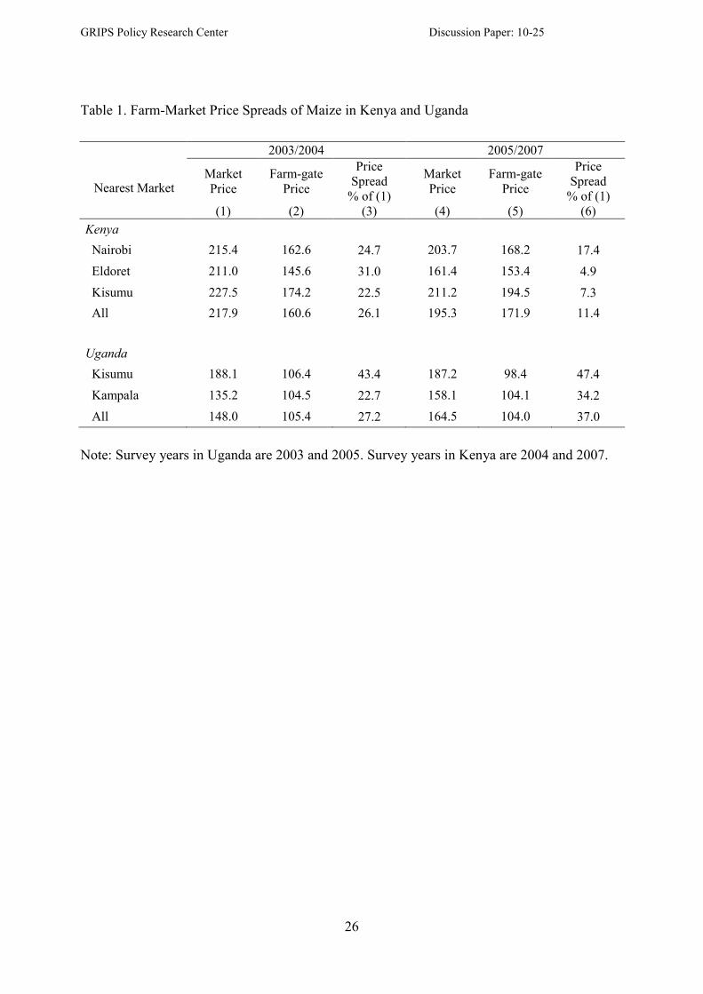
In Table 1, we find that the average maize market price in the two harvest seasons in

2004 is about USD 215 per ton in Nairobi. During the same period, the average farm-gate

maize price for farmers, who live closer to Nairobi than the other two maize markets in Kenya,

is USD 163 per ton. Thus, the farm-market price spread is about USD 52 per ton, which is

about 25 percent of the market price. In 2007, the average maize market price is USD 204, and

the farm-gate price is USD 168. Thus, the farm-market price spread is about 17 percent of the

market price.


14

As discussed earlier, Eldoret is located in a maize surplus area and usually has lower

maize prices than in Nairobi. In Table 1, we find that the average maize price is USD 211 per

ton in 2004 and USD 161 in 2007. These prices are lower than the Nairobi prices in both years,

especially in 2007. Because the 2006 maize harvest was especially good in Rift Valley, the

maize price declined in Eldoret, as we can see in Figure 2. The farm-gate price remains at just

below the market price and the price spread is only 5 percent of the market price.

In western Kenya, Kisumu is the largest city where a large quantity of maize is traded.

In Kisumu, the average maize market price is higher than the one in Nairobi in the harvest

seasons of 2004 and 2007: it is USD 228 in 2004 and USD 211 in 2007. The farm-gate price is

higher in this area also: it is USD 174 in 2004 and USD 195 in 2007. The price spread in 2004

is 22.5 percent of the market price. As in the Eldoret area, the price spread declines

considerably in 2007, to 7.3 percent in 2007. As a result, the average price spread for the whole

sample in Kenya declines from 26.1 percent in 2004 to11.4 percent in 2007.

In Uganda, the market maize price is much lower than in Kenya, as we have already

discussed in Section 2.2. The average maize price in Kampala is USD 135 in 2003 and 158 in

2005. The corresponding farm-gate price for maize farmers, who live closer to Kampala than

Kisumu, is USD 105 in 2003 and USD 104 in 2005. Thus, the price spread is about 22.7 and

34.2 percent in 2003 and 2005, respectively. For those Ugandan farmers who live closer to


15

Kisumu than Kamapala, the farm-gate price is USD 106 in 2003 and USD 98 in 2005. Thus,

compared with the market price in Kisumu, the price spread is about 43.4 and 47.4 percent in

2003 and 2005, respectively. Therefore, while Kenyan farmers who live close to Kisumu are

receiving farm-gate maize prices which are about 3 to 19 percent lower than the Kisumu price,

Ugandan farmers across the border are receiving farm-gate prices which are more than 40

percent below the same Kisumu price. Since Ugandan farmers are located far away from

Kisumu, the difference in distance to Kisumu may explain much of the difference. In order to

examine the price spreads across countries and regions, we need to control for the driving

hours to the nearest maize market from each household.

To analyze the relationship between the farm-market price spread and the driving time

to the nearest maize market, we first draw a simple plot between the price spread, expressed as

the percentage of the market price, and the driving time to the nearest maize market. To smooth

the measurement errors over the years, we pool the data over the years for each country.

According to Figure 4, the farm-market price spread is lower in Kenya than in Uganda. In

Kenya, the farm-market price spread is about 10 percent if maize farmers are located within

two driving hours to the nearest maize market. The farm-market price spread starts increasing

gradually to about 20 percent at five driving hours. In Uganda, even within one driving hour,

the farm-market price spread is already about 30 percent. As the distance becomes longer, the


16

price spread increases gradually to about 35 percent of the market price. The price spread

increases only by 5 percentage points over the five-driving hour distance in Uganda, while it

increases about 10 percentage points in Kenya over the same distance.

In Table 2, we divide the samples into three groups according to driving time to the

nearest market: 0 to 2 hours, 2 to 4 hours, and over 4 hours. As in the previous table, we further

divide the samples by the nearest market. In this table, we find that the price spread widens as

the distance to the nearest market increases. In the Nairobi area, the average farm-gate price is

about 20 percent below the market price at Nairobi. The price spread is about 16 percent if

maize farmers are located within a two-hour driving distance. The price spread somehow

declines slightly to 14 percent in the next distance group but increases to 28 percent in the

remote group (over 4 hours). In Eldoret and Kisumu areas, we also find that the price spread is

the largest in the most remote area, even though the second most remote group has the lowest

price spread in the Kisumu area. In Uganda, the relationship between the price spread and the

driving time to the nearest market is less clear. In the Kampala area, the price spread is larger

in the second and most remote areas than the least remote area, but the differences are small. In

the eastern Uganda area, which is closer to Kisumu than Kamapala, there are no households

who are within a two hour driving distance from a market. In the second most remote area, the

price spread is about 50 percent of the market price in Kisumu, implying that the farm-gate


17

price is about half of the market price. This is much lower than what Kenyan farmers who are

located within the same time range from Kisumu receive. Their price spread is about 12

percent of the market price. Among the most remote groups, however, maize farmers in Kenya

and Uganda near Kisumu receive about the same level of the farm-gate price, which is about

60 percent of the market price, as indicated by the price spread of about 40 percent.

These findings suggest that the low farm-gate price compared with the market price in

Uganda is not only because of the long distance to the nearest market but other factors, such as

market structure and competition, matter. For instance, the unit price of maize may differ

depending on the total volume of sales, where large maize farmers fetch a higher per unit price

from maize traders than small maize farmers. Thus, we need to control for household

characteristics. As we discussed in Section 2.2, there may be more maize traders in Kenya than

in Uganda and maize is traded more often. If maize marketing in Uganda improves its

efficiency to the Kenyan level so farm-gate prices would rise by 10 percentage points

compared to the market price, then the maize farmers in the country will gain USD 14 to USD

18 per ton. Since the distance to market is not the only factor that affects the farm-gate to

market price ratio, we further explore the determinants of the ratio through regression analyses.


18

5. Estimation Models and Variables

To measure the marketing efficiency across countries and over time, we use the

farm-market price spread measured as the percentage of the market price. The farm-market

price spread has been used in many studies before, as surveyed in Fackler and Goodwin (2002).

We use the percentage figure, instead of the price spread itself, because we want to eliminate

inflation and exchange factors from our measure of efficiency. Thus, the regression model we

estimate is

PSi = f (Mi, Ei, Hi, Y, S), (2)

where PSi is the farm-market price spread measured as the percentage of the market price; Mi is

the market access variable measured by the driving time from household i to the nearest maize

market; Ei is a set of agro-ecological variables; Hi is a set of household characteristics of

household i; Y is the year dummy for the second round; and S is the season dummy for the

second season. PSi is defined as

PSi, = [(piM - pi

F)/pi

M ] x 100, (3)

where piM is the market price of maize at the nearest maize market for household i and pi

F is the

farm-gate price of household i. The dependent variable is always above zero in our data and


19

can be over 100 when the farm-gate price exceeds the market price, which occurs in our data

set. Thus, we use the OLS model to estimate the regression function.

The agro-ecological variables include PPE (Precipitation over Potential

Evapotranspiration ratio), altitude, soil fertility, and population density. The PPE is used as an

index for agro-climate conditions such as rainfall and temperature (a higher PPE denotes a

greater agricultural potential), which is obtained from the data base contained in the Almanac

Characterization Tool (Corbett, 1999). When we conducted community surveys in 2003 and

2005, we obtained the GIS coordinates of each community center. Thus, the altitude is

measured at the community level. In addition to these variables, we include a soil fertility

variable in the model. As an index of the soil fertility, we use the soil organic matter (SOM)

content. Because the SOM is available for just the sub-samples, we could estimate the models

with the sub-samples only. This method, however, may create selection biases because the

sub-samples with the soil fertility data are not selected randomly. Instead, we replace all the

soil related variables with zero and include an additional dummy variable for those households

without soil data. To assure that our approach provides robust estimates, we estimate the same

model for all the households and the reduced sample.

The household characteristics include human capital and asset variables. The human

capital variables include the age, education levels, and gender of the household heads. For


20

household assets, we include own land size in hectares and the value of household farm

equipments, furniture, transportation means, communication devices, and other household

assets. Because the size and the soil fertility of the land are separately included in the model,

we do not add the value of land to the total asset value.

6. Results

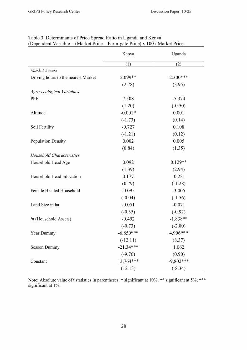
The estimated coefficient of the driving time in column 1 of Table 3 is 2.1 for Kenya,

suggesting that the maize price spread increases by 2.1 percentage points against the market

price as the driving time increases by one hour. In Figure 4, we find that the price spread

increases from 10 to 20 percent of the market price as the driving time increases by 5 hours in

Kenya. Thus, the estimation result is largely consistent with what we find in Figure 1 for

Kenya. The estimation result for Uganda is similar to that for Kenya: one additional driving

hour increases the price spread by 2.3 percentage points against the market price in Uganda.

As we have seen in Figure 4, maize farmers in Uganda who are located five hours away from

the nearest market receive at least a 10 percentage-point lower maize price than maize farmers

who live near the market. These findings indicate that the marginal transportation cost

associated with an increase in driving time affects the price spread equally between Kenya


21

and Uganda, which may be taken to imply that local maize markets function well over the two

countries.

None of the agro-ecological variables has significant coefficients. Thus, the

agro-ecological variables do not affect the price spread between the farm-gate price and the

market price, although they may affect the maize output price levels. Moreover, none of the

household characteristics has significant coefficients in Kenya. Thus, as far as the maize

market in Kenya is concerned, there is no indication of market imperfections, which supports

Hypothesis 1 discussed in Chapter 1 that markets function well. In Uganda, young

household heads and those who have more households assets have lower price spreads, i.e.,

higher farm-gate prices than others. One possible way for them to receive a higher price is to

transport maize to a market where they can fetch a higher price. This is possible if the maize

market is not well developed in Uganda. If the maize market is well developed, individual

farmers do not need to transfer maize to a market because traders can do so at a lower cost

than individual farmers. Such market imperfections in Uganda may explain why the price

spread is much larger in Uganda than in Kenya, which is shown in Figure 4.

7. Conclusions


22

To reduce poverty in rural areas, rural communities need to be integrated with markets

so that they can receive high and stable returns to their agricultural products, thereby becoming

less vulnerable to production shocks. Although there have been many studies that test market

integration across markets by using time series price data, few studies have examined the price

spread between market and farm-gate prices across countries by using panel data. Because poor

transportation infrastructure is considered to be a major factor behind the high marketing costs

in Africa, we examine the relationship between the farm-market price spread and driving time

from each sample household to the nearest maize market where we have monthly maize price

data. The findings in this chapter indicate that there are substantial price spreads between farm

gates and markets, which strongly suggests that the farm gate price can be raised significantly

by improving road conditions.

We also found that in both countries, the price spread increases equally by 2

percentage points for one additional hour of driving time from the nearest maize market.

Furthermore, we found that agro-ecological variables and household characteristics are

generally insignificant in the price spread regressions, except for a few variables in Uganda.

Although far from concrete, these findings indicate that local maize markets function well

except in Uganda where there still remain some market imperfections. In order to reduce


23

rural poverty, policies to reduce transportation costs and facilitate market competition are

called for, particularly in Uganda.


24

References

Ariga, J., Jayne, T. S. & Njukia, S. (2010). Staple Food Policies in Kenya, a Paper Prepared for

the COMESA policy seminar on Variation in Staple Food Prices: Causes, Consequence,

and Policy Options, the Comesa-MSU-IFPRI African Agricultural Marketing Project

(AAMP), Maputo, Mozambique, 25-26 January 2010.

Barrett, C. B. (2008). Smallholder Market Participation: Concepts and Evidence from Eastern

and Southern Africa. Food Policy, 33, 299-317.

Badiane, O. & Shively, G. E. (1998). Spatial Integration, Transport Costs and the Resource of

Local Prices to Policy Changes in Ghana. Journal of Development Economics, 56,

411-431.

Benson, T., Mugarura, S. & Wanda, K. (2008). Impacts in Uganda of Rising Global Food

Prices: the Role of Diversified Staples and Limited Price Transmission. Agricultural

Economics, 39, 513-524.

Byerlee, D., Jayne, T. S. & Myers, R. J. (2006). Managing Food Price Risks and Instability in a

Liberalizing Market Environment: Overview and Policy Options. Food Policy 31,

275-287.

Campenhout, B. V. (2007). Modeling Trends in Food Market Integration: Method and an

Application to Tanzania Maize Markets. Food Policy, 32, 112-127.

Corbett, J. C. (1999). The Almanac Characterization Tool, Version 2.01. Characterization,

Assessment and Applications Group, Blackland Research Center, TAES, Texas A&M

University System, a CDROM publication.

Fackler, P. L. & Goodwin, B. K. (2002). Spatial Price Analysis. In B.L. Gardner and G.C.

Rausser (Eds.), Handbook of Agricultural Economics. Amsterdam: Elsevier Science.

Fafchamps, M. (2004) Market Institutions in Sub-Saharan Africa: Theory and Evidence.

Cambridge: MIT Press.

Faminow, M. D. & Laubscher, J. M. (1991). Empirical Testing of Alternative Price Spread

Models in the South African Maize Market. Agricultural Economics, 6, 49-66.

Goletti, F. & Babu, S. (1994). Market Liberalization and Integration of Maize Markets in

Malawi. Agricultural Economics, 11, 311-324.

Jayne, T. S., Myers, R. J. & Nyoro, J. (2008). The Effects of NCPB Marketing Policies on

Maize Market Prices in Kenya. Agricultural Economics, 38, 313-325.


25

Jayne, T. S., Zulu, B. & Nijhoff, J. J. (2006). Stabilizing Food Markets in Easter and Southern

The Effects of NCPB Marketing Policies on Maize Market Prices in Kenya.

Agricultural Economics, 38, 313-325.

Krishana, A. (2004). Escaping Poverty and Becoming Poor: Who Gains, Who Loses, and

Why? World Development, 32, 121-136.

Lutz, C., Kuiper, W. E. & van Tilburg, A. (2006). Maize Market Liberalisation in Benin: A

Case of Hysteresis. Journal of African Economies, 16, 102-133.

Minot, N. (2007). Are Poor, Remote Areas Left Behind in Agricultural Development: The

Case of Tanzania. Journal of African Economies, 17, 239-276.

Negassa, A., Myers, R. & Gabre-Madhin, E. (2004). Grain Marketing Policy Changes and

Spatial Efficiency of Maize and Wheat Markets in Ethiopia. MTID Discussion Paper 66,

International Food Policy Research Institute.

Poulton, C., Dorward, A. & Kydd, J. (1998). The Revival of Smallholder Cash Crops in Africa:

Public and Private Roles in the Provision of Finance. Journal of International

Development, 10, 85-103.

Rashid, S. (2004). Spatial Integration of Maize Markets in Post-liberalised Uganda. Journal of

African Economies, 13, 102-133.

Ravallion, M. (1986). Testing Market Integration. American Journal of Agricultural

Economics, 68, 102-109.


26

Table 1. Farm-Market Price Spreads of Maize in Kenya and Uganda

Nearest Market

2003/2004 2005/2007

Market

Price

Farm-gate

Price

Price

Spread

% of (1)

Market

Price

Farm-gate

Price

Price

Spread

% of (1)

(1) (2) (3) (4) (5) (6)

Kenya

Nairobi 215.4 162.6 24.7 203.7 168.2 17.4

Eldoret 211.0 145.6 31.0 161.4 153.4 4.9

Kisumu 227.5 174.2 22.5 211.2 194.5 7.3

All 217.9 160.6 26.1 195.3 171.9 11.4

Uganda

Kisumu 188.1 106.4 43.4 187.2 98.4 47.4

Kampala 135.2 104.5 22.7 158.1 104.1 34.2

All 148.0 105.4 27.2 164.5 104.0 37.0

Note: Survey years in Uganda are 2003 and 2005. Survey years in Kenya are 2004 and 2007.


27

Table 2. Maize Price Spreads by Driving Time to the Nearest Maize Market

All Driving Hours to the Nearest Maize Market

0 to 2 Hours 2 to 4 Hours Over 4 Hours

(1) (2) (3) (4)

Kenya

Nairobi 20.4 15.6 14.0 28.1

Eldoret 19.7 15.4 18.8 22.1

Kisumu 15.4 21.4 11.5 39.2

All 18.7 17.6 13.1 25.8

Uganda

Kisumu 45.2 n.a. 49.5 43.0

Kampala 29.2 25.3 29.8 29.3

All 32.7 25.3 32.9 33.6


28

Table 3. Determinants of Price Spread Ratio in Uganda and Kenya

(Dependent Variable = (Market Price – Farm-gate Price) x 100 / Market Price

Kenya Uganda

(1) (2)

Market Access

Driving hours to the nearest Market 2.099** 2.300***

(2.78) (3.95)

Agro-ecological Variables

PPE 7.508 -5.374

(1.20) (-0.50)

Altitude -0.001* 0.001

(-1.73) (0.14)

Soil Fertility -0.727 0.108

(-1.21) (0.12)

Population Density 0.002 0.005

(0.84) (1.35)

Household Characteristics

Household Head Age 0.092 0.129**

(1.39) (2.94)

Household Head Education 0.177 -0.221

(0.79) (-1.28)

Female Headed Household -0.095 -3.005

(-0.04) (-1.56)

Land Size in ha -0.051 -0.071

(-0.35) (-0.92)

ln (Household Assets) -0.492 -1.838**

(-0.73) (-2.80)

Year Dummy -6.850*** 4.906***

(-12.11) (8.37)

Season Dummy -21.34*** 1.062

(-9.76) (0.90)

Constant 13,764*** -9,802***

(12.13) (-8.34)

Note: Absolute value of t statistics in parentheses. * significant at 10%; ** significant at 5%; ***

significant at 1%.


29

Figure 1. Map of Four Maize Markets and Sample Households in Kenya and Uganda


30

Figure 2. Monthly Maize Price at Nairobi and Eldoret from January 2001 to January 2007

0

50

100

150

200

250

300Jan01

Apr01

Jul01

Oct01

Jan02

Apr02

Jul02

Oct02

Jan03

Apr03

Jul03

Oct03

Jan04

Apr04

Jul04

Oct04

Jan05

Apr05

Jul05

Oct05

Jan06

Apr06

Jul06

Oct06

Jan07

Nairobi : KE Eldoret : KE


31

Figure 3. Monthly Maize Price at Kisumu and Kampala from January 2001 to January 2007

0

50

100

150

200

250

300Jan01

Apr01

Jul01

Oct01

Jan02

Apr02

Jul02

Oct02

Jan03

Apr03

Jul03

Oct03

Jan04

Apr04

Jul04

Oct04

Jan05

Apr05

Jul05

Oct05

Jan06

Apr06

Jul06

Oct06

Jan07

Kisumu : KE Kampala : UG


32

Figure 4. Farm-Market Price Spread as a Percentage of Market Price by the Driving Time to

the Nearest Marker in Hours in Kenya and Uganda

Kenya

Uganda

0

10

20

30

40

Price Spread as % of Market Price

0 2 4 6 8Driving Hours to the Nearest Maize Market

the maize farmthe maize farm- ---market price … · the maize farmthe maize farm- ---market price...

Documents