The Magnetic Pendulum

Uzair Abdul Latif, Junaid Alam and Muhammad Sabieh Anwar

LUMS School of Science and Engineering

Version 2015-1

May 22, 2015

Nonlinearity is a profound concept in the study of physical systems. The characteristics of seemingly

very simple systems may turn out to be extremely intricate due to non-linearity. The study of chaos

also begins with the study of such simple systems. The magnetic pendulum can be one such system.

A pendulum is one of the simplest and diverse systems in terms of its mathematical basis and the

range of �elds of science that it can relate to. Without doubt, it is a gift of re ective simplicity for

reductionist science. With slight modi�cations, it can exhibit even exotically insightful phenomena,

chaos being one of them. In this experiment, we will explore the notion of nonlinear and chaotic

dynamics using a \magnetic pendulum".

KEYWORDS

Determinism � Chaos � Supersensitivity � Phase Portrait � Poincare Map � Attractor � Resonance �

Rotary motion sensor.

PREREQUISITE EXPERIMENT: Chasing Chaos with an RL-Diode Circuit

Contents

1 Objectives 2

2 Introduction 3

1

3 Apparatus 3

4 The Experiment 4

4.1 Exploring Non-Linearities . . . . . . . . . . . . . . . . . . . . . . . . . . . . . . . . . 5

4.1.1 Simulating the Simple Pendulum . . . . . . . . . . . . . . . . . . . . . . . . . 5

4.1.2 Experiment . . . . . . . . . . . . . . . . . . . . . . . . . . . . . . . . . . . . 6

4.2 Varying the Experimental Parameters . . . . . . . . . . . . . . . . . . . . . . . . . . 7

4.2.1 Varying the distance, d , between the magnets . . . . . . . . . . . . . . . . . 7

4.2.2 Obserivng the Sensitivity of the System by Varying the Initial Conditions . . . 20

4.3 Observing Amplitude Hysteresis in Pendulum's Behavior . . . . . . . . . . . . . . . . 21

1 Objectives

In this experiment, we will discover:

1. how apparently simple systems can be highly non-linear and exhibit a complex behavior under

certain conditions,

2. the physical structure of dynamical systems, and

3. the conditions and consequences of the notion of super-sensitivity and its relationship with chaos

through simulation and experiment.

References

[1] Yaakov Kraftmakher, \Experiments with a magnetically controlled pendulum", Eur. J. Phys. 28,

1007-1020, (2007)

[2] A. Siahmakoun, V. A. French, J. Patterson, \Nonlinear dynamics of a sinusoidally driven pendulum

in a repulsive magnetic �eld", Am. J. Phys. 65, (1997).

[3] Priscilla W. Laws, \A unit of oscillations, determinism and chaos for introductory physics stu-

dents", Am. J. Phys. 72, (2003).

[4] Junaid Alam, M. Sabieh Anwar, \Chasing Chaos with an RL-Diode Circuit",

http://physlab.lums.edu.pk/

2

[5] Loius A. Pipes, Lawrence R. Harvill, \Applied Mathematics for Engineers and Physicists", Third

Edition, International Student Edition, McGraw-Hill Kogakusha Ltd. pp. 598-601, (1970)

2 Introduction

Almost all of the known physical systems are essentially nonlinear. Yet, for simplicity, they can be

treated as linear systems within some operating constraints. The magnetic pendulum is one such

system. It is essentially a nonlinear system. So, it can help us to look into nonlinear phenomena such

as chaos.

3 Apparatus

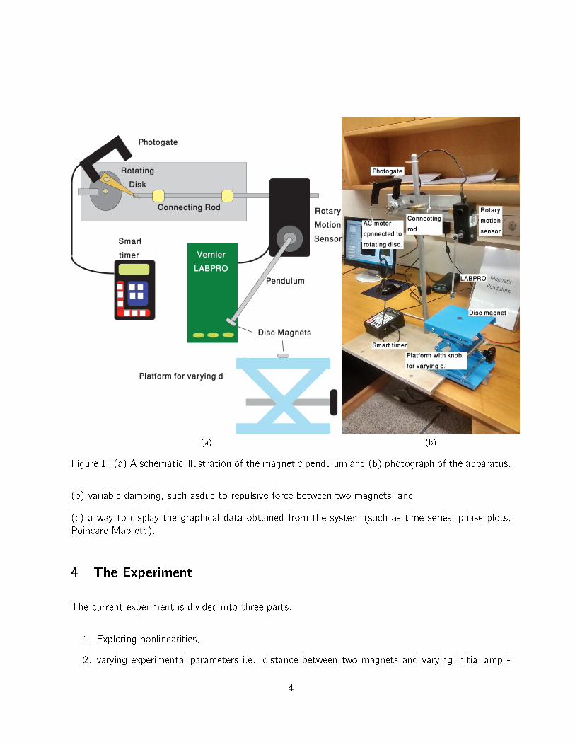
The schematic of our homebuilt apparatus is shown in Figure 1 (a) while (b) is a photograph.

Basically an AC induction motor has been used as the driving device. We use it for its readily available

power supply and for its ease in speed control, which is simply achieved by turning the varying the

input voltage.

The ywheel and connecting rod assembly converts the circular motion of motor's shaft to an approx-

imately linear harmonic motion of the bearing-rod assembly to which the pendulum and rotary motion

sensor are attached.

Think: What is the advantage of using a ywheel?

The Vernier Rotary Motion Sensor (RMS) encodes the angular information of the shaft into a digital

stream and sends it to your LabVIEW program through LabPro. This information can then be used

in Matlab for further processing.

A small idential disc magnet provides the magnetic �eld to interact with that of the small magnet at

the end of pendulum. In this way, we can control the magnitude and nature of the restoring torque

and hence the nonlinearity of pendulum.

Both the magnets are kept with their same magnetic poles facing each other so that both of them

repel each other.

Design Idea: Can you design a better setup to meet the same qualitative requirements?

Note that the magnetic pendulum capable of exhibiting chaotic dynamics is required to ful�ll the

following demands:

(a) variable amplitude and frequency of the driving force, and

3

Photogate

Vernier

LABPRO

Smart

timer

Rotating

Disk

Connecting Rod Rotary

Motion

Sensor

Pendulum

Platform for varying d

Disc Magnets

(a)

Photogate

Smart timer

Rotary

motion

sensor

Disc magnet

Platform with knob

for varying d.

Connecting

rodAC motor

cpnnected to

rotating disc.

LABPRO

(b)

Figure 1: (a) A schematic illustration of the magnetic pendulum and (b) photograph of the apparatus.

(b) variable damping, such asdue to repulsive force between two magnets, and

(c) a way to display the graphical data obtained from the system (such as time series, phase plots,

Poincare Map etc).

4 The Experiment

The current experiment is divided into three parts:

1. Exploring nonlinearities,

2. varying experimental parameters i.e., distance between two magnets and varying initial ampli-

4

tudes to study the sensitive behaviour of the pendulum. The e�ects will be studied both through

simulation and through practical experiment, and

3. plotting a graph of maximum amplitude against angular frequency of the driving rod and ob-

serving the phenomena of hysteresis and bistability.

4.1 Exploring Non-Linearities

4.1.1 Simulating the Simple Pendulum

We start o� this experiment through a pre-lab exercise exploring nonlinearity. Of course, the purpose

is to see how a simple pendulum can become nonlinear. Tn this regime, the assumption that the time

period is independent of the initial pendulum breaks down.

If we ignore friction a simple pendulum's equation of motion can be written as:

�� +g

lsin(�) = 0 (1)

If we make the small angle approximation i.e. sin(�) � � the we get:

�� +g

l� = 0 (2)

Here, � is the angular displacement of the pendulum of the length, l , and g is the acceleration due to

gravity.

Question What factors control the time period of the pendulum in the case of small angles? Does

time period depend on the initial amplitude from which the pendulum is displaced? Derive Eq. (1)

from Newton's force equation.

For the large amplitude case we can rearrange and integrate Equation (2) to give us the following

formula for time period of a pendulum:

T (�o) = 4

√l

gK(k) (3)

where,

K(k) =

∫ �

2

0

d�√1� k2 sin2 �

(4)

5

here k = sin �o2and sin �

2= k sin�. It can also be observed that the time period, T , is a function

of �o which is the initial amplitude or initial point of release of the pendulum. Furthermore K(k) is

called the complete the complete elliptic integral of the �rst kind and can be easily tabulated through

Matlab. If you type in the following set of commands in Matlab1:

>> theta o=(20/180)*pi;

>> k=sin(theta o/2);

>> a=pi/2;

>> int('1/sqrt(1-k*k*sin(x)*sin(x))',0,a)

Here thetao is the initial amplitude of the pendulum de�ned in radians.This command will return you

EllipticK(k2) which is actually the answer of the integral. In order to calculate the exact value you

will of the integral type in the following command:

>> Y=mfun('EllipticK',k2);

Here Y would be your value of the integral for that particular �o . Substitute the value of the integral

back in the time period formula and the value of the time period can be calculated for that speci�c

�o . For further clarity please refer to [5]. The reference is also available on the experiment webpage.

Exercise Plot a graph time period versus �o . Vary values of �o from 0o to 90o . Take the value of l

to be 0:1338 m. At what point would you say the transition from linearity to non-linearity occurs?

Question With the help of [5], derive Eq. (4).

4.1.2 Experiment

Now you will actually try to see the transition from linearity to non-linearity by measuring time periods

for varying initial amplitudes of the pendulum. You will use a stop watch to measure the time period

and ou will use your own judgment call to estimate the value for �o or the point of release of the

pendulum.

The pendulum will be allowed to oscillate freely and the magnet below the pendulum will be removed

for this part of the experiment.

Exercise Measure the time period of the pendulum for varying initial amplitudes. How do your

experimental and simulation results compare?

1These commands require Matlab's Symbolic Math Toolbox. Type 'ver' in your Matlab command window to check

and see if you have this toolbox.

6

4.2 Varying the Experimental Parameters

4.2.1 Varying the distance, d , between the magnets

Precaution: Never run the motor at high speeds. It may damage the apparatus. Start from very low

speeds and gradually increase when needed. If the motor instantaneously gains speed, switch it o�

immediately.

In this part of the experiment you will steadily decrease the distance, d , between the two magnets

and observe the changes that occur in the phase portrait of the pendulum for each distance where

d is the minimum distance between the two magnets. The e�ort will be basically focused at trying

to �nd out that how and when the system gets trapped in a lopsided attractor and how does it jump

between the two equilibrium positions (or attractors). One of the aims would also be to �gure out

that at what point does the pendulum exhibit chaotic behavior. In this section, all the phase portraits

will be plotted using Matlab.

Fdriver

Fgravity

Fmagnetic

rθ

hθ

m1

m2

Lθ

d

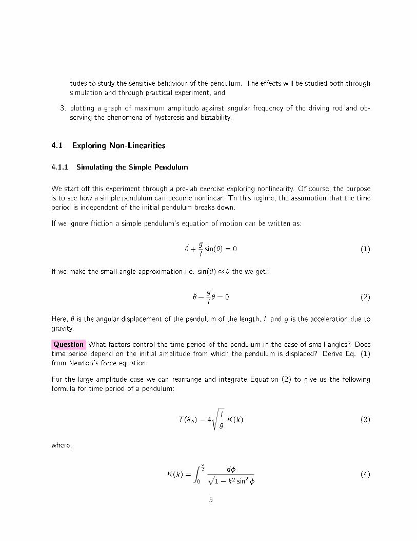
Figure 2: Schematic diagram of the physical pendulum and the forces acting on it. The distance d is

between magnets when the pendulum is in the resting position. The thick arrows show the magnetic

moment vectors. The angle � is measured with the rotary motion sensor.

4.2.1.1 Simulating the Magnetic Pendulum

Once again, we will gain insight by simulating the motion of our pendulum in Matlab. For that we will

need to know the equation of motion of the pendulum that will be numerically solved. The motion

exhibited by our pendulum is of the rotational kind so if we can write an equation describing all the

7

torques acting on a pendulum at any point we can derive its equation of motion. Figure 2 shows the

various torques acting on the pendulum, where upon the torques can be derived.

Using Newton's Second Law we can write:

Id2�

dt2= ��i (5)

where I is the moment of inertia of the pendulum and ��i is the vector sum of all the torques acting

on the pendulum and is given by:

��i = �grav ity + �dr iver + �damping + �magnetic (6)

Therefore we are now able to arrive at the following set of di�erential equations:

ML2

3_! = �

L

2Mg sin � + Tdr iver sin(t)� ! +

j�j

�L�o

4�

m1m2

r2�� cos

(j�j+ arctan

(�

∣∣∣∣ h�

L sin �

∣∣∣∣))(7)

_� = ! (8)

Where,

Fmagnetic =�o

4�

m1m2

r2�r̂ (9)

Equation (9) assumes a Coulomb-like inverse square law between two magnetic moments m1 and m2

separated by a a distance r�. The unit vector r̂ points radially away from the line joining the two

magnets and indicates the direction of the magnetic force at some distance.

Here r� =√(L sin �)2 + h2� and h� = d +L(1� cos �). The variables r� and h� are shown in Figure 2.

In this case �o is the permeability of vacuum, L is the length of the pendulum, M is the mass of

the pendulum, g is the gravitational acceleration, Tdr iver is the maximum value of the periodic torque

produced by the horizontal displacement of the pivot, is the angular frequency of the driver and

is the damping constant.

Exercise Derive each term of Equation (7). Provide an explanation where possible.

Equation (7) can be simpli�ed and rewritten as:

8

_! = �A sin � + B sin(t)� C! +j�j

�

E

r2�� cos

(j�j+ arctan

(�

∣∣∣∣ h�

L sin �

∣∣∣∣)) (10)

where A, B, C and E are constant coe�cients that depend only the physical constants associated

with the system. We are going values of these constants given for the pendulum system in [2].

The following parameter values and initial conditions will be used for the Matlab simulations: A =

110 s�2, B = 0:01 s�2, C = 0:001 s�1, E = 0:2 m2s�2, �(0) = 0:2 rad and !(0) = 0. All these

values and conditions will be kept constant throughout all simulation runs.

Now to start work on the simulation download the pendode1.m �le from the web page of the exper-

iment. Open the m-�le and you will see the following:

Figure 3: The pendode1.m �le.

1. Write your values for parameters A, B, C and E. You may calculate values of these parameters

for your own pendulum system and use them.

2. Write the two Equations (8) and (7), respectively in front of dy(1)=; and dy(2)=;. In our

simulation the de�ned variables are y(1) � !, y(2) � �, dy(1) � _! and dy(2) � _�. For

example for writing _� = 10! � 2 you will write dy(2)=10y(1)-2;

9

3. Set the value of d for which want to run your simulation. After the parameter values have been

set and the equations have been de�ned you will now initiate the simulation by typing in the

following commands in Matlab command window:

NOTE: The pendode1.m �le should be saved in the current directory of Matlab because only

then will you be able to call that �le using Matlab's command window.

>> options = odeset('RelTol',2.22045e-14,'AbsTol',[1e-14 1e-14]);

>> [T,Y] = ode113(@pendode1,[0 1000],[0 0.2],options);

Here ode113 is being called on to solve the system of di�erential equations which you have

de�ned in pendode1.m. The function ode113 is one of the many di�erential equation solvers

that come with Matlab. The interval [0 1000] indicates the time in seconds (or the values of

time vector, T ) for which the simulation will be run. In real time, the ode113 would take about

10-20 s to solve the equation for the speci�ed time range of 1000 s. The vector [0 0:2] indicates

the initial conditions of our two variables, y(1) � ! and y(2) � �.

The options command sets the relative and absolute tolerance levels of the ode solver for our

two parameters: !, �. As we are looking at a very sensitive pendulum system therefore the

tolerance levels have been set extremely low to give us a high degree of accuracy in our results.

These tolerance levels have been adjusted after trials.

After �nishing o� its processing the ode solver will return to you two vectors in the Matlab

Variable Workspace : a time vector T and one vector Y which would have two columns each

corresponding to our two variables, ! and �.

4. Plot the waveform time series of �.

NOTE: In our phase portrait and time series plots we will only be plotting that part of our data

where the pendulum has reached a steady state. So it will have to be ensured that for any set

of data of � being used to plot there are no transient states present. It will be your judgment

call in each case to tell when the simulation reaches the steady state.

5. Plot the phase portrait using the same set of data of � which you used to make time series.

HINT: To plot the phase portrait you will need to plot ! vs �. Here ! is basically ���T

. So

�� would be simply obtained by using the di�() command. Moreover, �T would have to be

inferred in the same way from your corresponding T vector data set.

6. A set of sample results for varying distances are shown in the following pages. Here d1 > d2 >

d3 > d4 > d5 > d6. The step size between each of these distances is not necessarily equal.

You will need to reproduce these results and also �nd out a value of d for which the pendulum

exhibits chaotic behavior. All the times in the in the time series graphs have been 'zeroed',

starting from zero to maintain consistency.

10

−0.2 −0.15 −0.1 −0.05 0 0.05 0.1 0.15 0.2−1.5

−1

−0.5

0

0.5

1

1.5

θ (rad)

ω (

rad/

s)

d1

(a)

0 2 4 6 8 10 12−0.2

−0.15

−0.1

−0.05

0

0.05

0.1

0.15

0.2

Time (s)

θ (r

ad)

d1

(b)

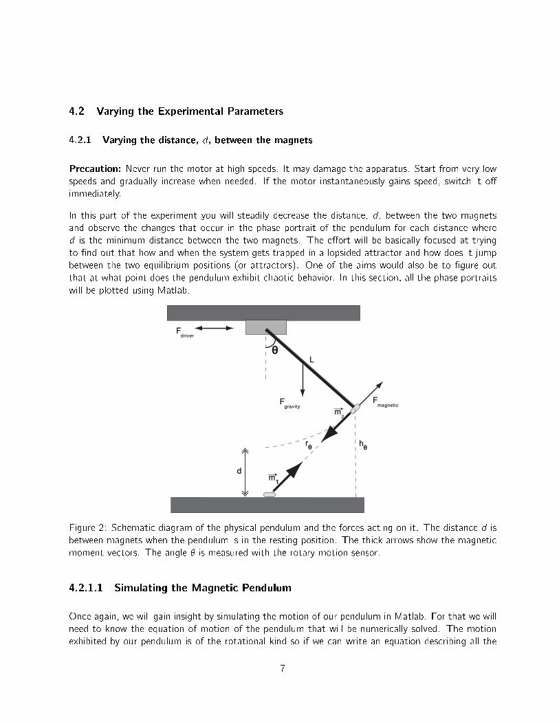
Figure 4: (a) Phase plot and (b) time series showing periodic motion for d1. For relatively large d ,

the motion is approximately similar to a simple pendulum.

−0.2 −0.15 −0.1 −0.05 0 0.05 0.1 0.15 0.2−0.4

−0.3

−0.2

−0.1

0

0.1

0.2

0.3

0.4

ω (

rad/

s)

θ (rad/s)

d2

(a)

0 2 4 6 8 10 12 14 16 18−0.2

−0.15

−0.1

−0.05

0

0.05

0.1

0.15

0.2

d2

θ (r

ad)

Time (s)

(b)

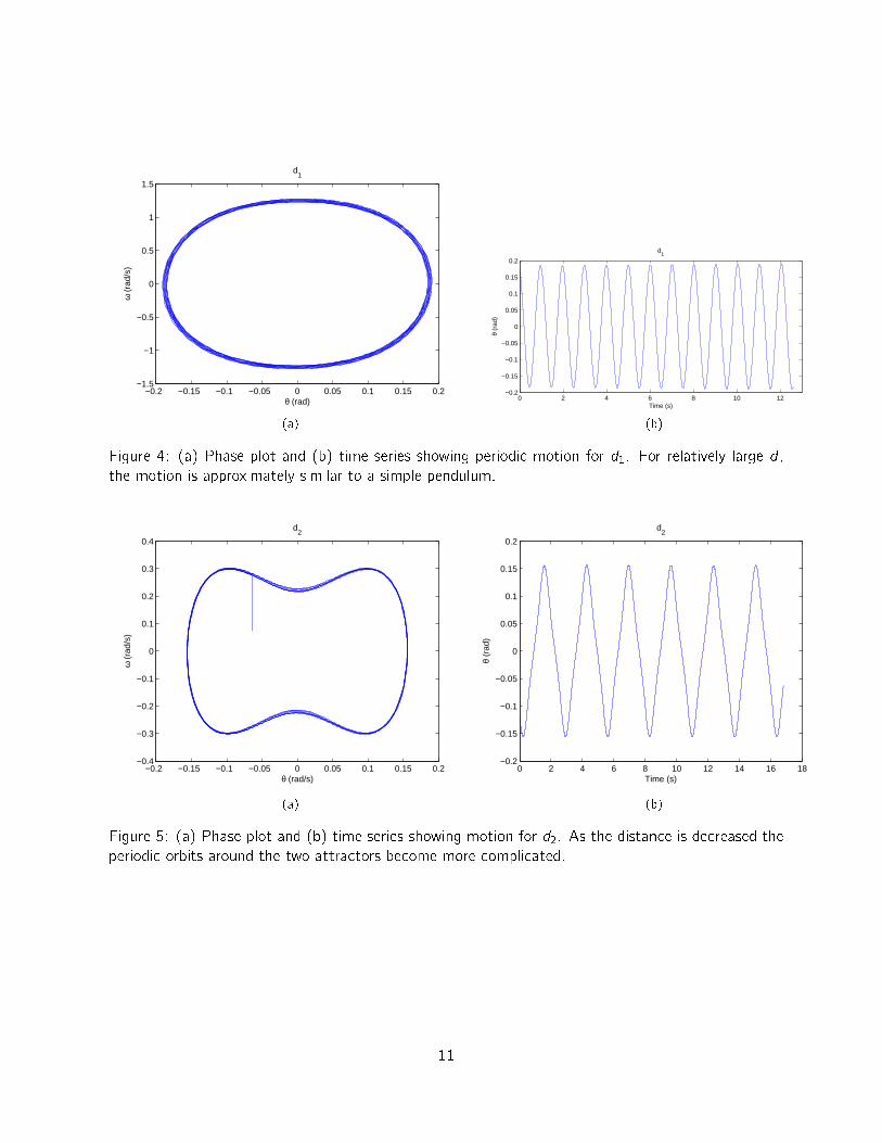
Figure 5: (a) Phase plot and (b) time series showing motion for d2. As the distance is decreased the

periodic orbits around the two attractors become more complicated.

11

−0.25 −0.2 −0.15 −0.1 −0.05 0 0.05 0.1 0.15 0.2−0.25

−0.2

−0.15

−0.1

−0.05

0

0.05

0.1

0.15

0.2

0.25

θ (rad)

ω (

rad/

s)

d3

(a)

0 5 10 15−0.25

−0.2

−0.15

−0.1

−0.05

0

0.05

0.1

0.15

0.2

0.25

d3

θ (r

ad)

Time (s)

(b)

Figure 6: (a) Phase plot and (b) time series showing motion for d3. The repulsive force starts slowing

the magnet down when it passes between the two attractors. This e�ect is clearly evident in the

'pinching' of the phase portraits near � � 0 rad

−0.2 −0.15 −0.1 −0.05 0 0.05 0.1 0.15 0.2−0.4

−0.3

−0.2

−0.1

0

0.1

0.2

0.3

0.4

θ (rad)

ω (

rad/

s)

d4

(a)

0 20 40 60 80 100 120−0.2

−0.15

−0.1

−0.05

0

0.05

0.1

0.15

0.2

d4

θ (r

ad)

Time (s)

(b)

Figure 7: (a) Phase plot and (b) time series showing periodic motion for d4. It can be seen in the

time series the pendulum exhibits chaotic motion in the beginning and then gets stuck in the attractor

on the right.

Exercise Select a value of d where the simulation exhibits chaotic motion and plot its phase portrait.

12

−0.15 −0.1 −0.05 0 0.05 0.1 0.15−0.1

−0.05

0

0.05

0.1

θ (rad)

ω (

rad/

s)

d5

(a)

0 2 4 6 8 10 12 14 16−0.2

−0.15

−0.1

−0.05

0

0.05

0.1

0.15

0.2

d5

θ (r

ad)

Time (s)

(b)

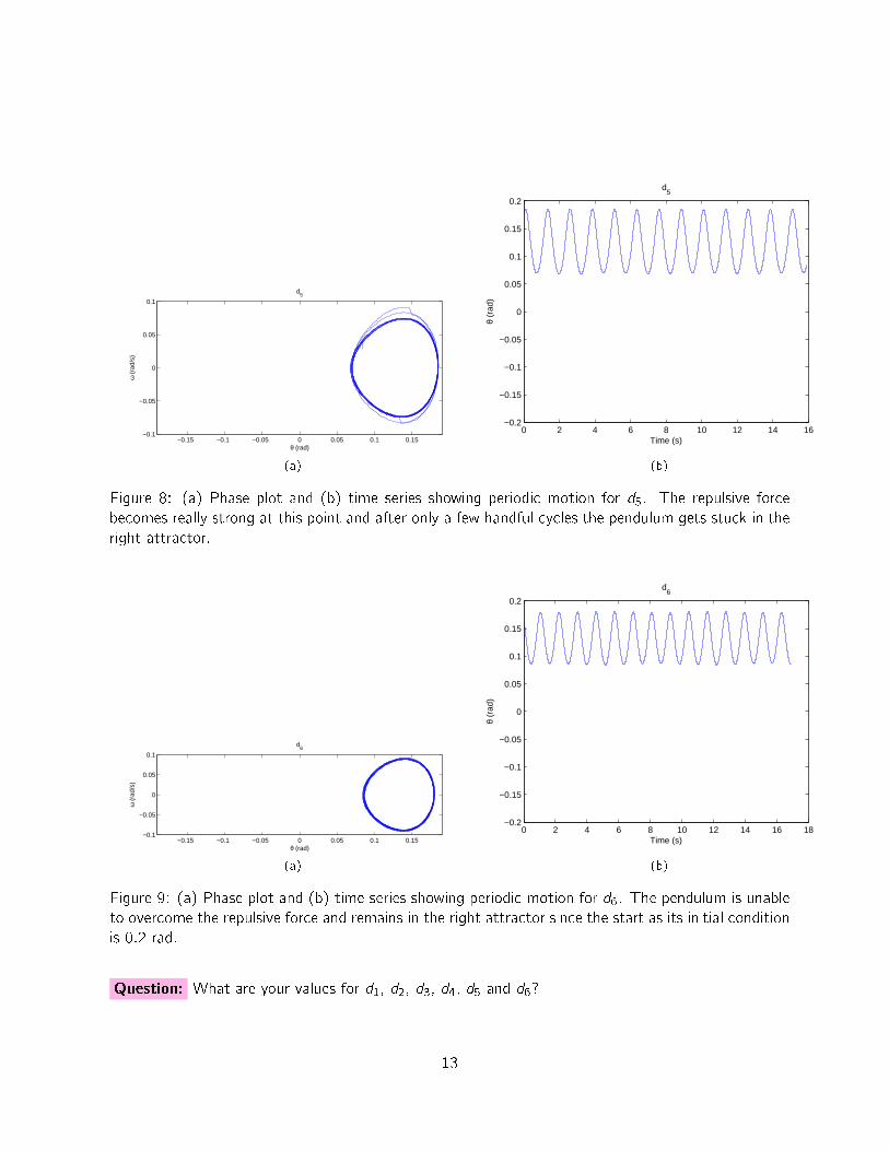
Figure 8: (a) Phase plot and (b) time series showing periodic motion for d5. The repulsive force

becomes really strong at this point and after only a few handful cycles the pendulum gets stuck in the

right attractor.

−0.15 −0.1 −0.05 0 0.05 0.1 0.15−0.1

−0.05

0

0.05

0.1

ω (

rad/

s)

θ (rad)

d6

(a)

0 2 4 6 8 10 12 14 16 18−0.2

−0.15

−0.1

−0.05

0

0.05

0.1

0.15

0.2

d6

θ (r

ad)

Time (s)

(b)

Figure 9: (a) Phase plot and (b) time series showing periodic motion for d6. The pendulum is unable

to overcome the repulsive force and remains in the right attractor since the start as its initial condition

is 0:2 rad.

Question: What are your values for d1, d2, d3, d4, d5 and d6?

13

4.2.1.2 The Experiment

In this section, we will practically verify the e�ect of successively decreasign d on ht behaviour of the

magnetic pendulum.. For that �rst you will need to �nd out the resonant frequency of our pendulum.

When the resonant frequency is known you will try to replicate the phase portraits at varying distances

that you obtained from the simulation. For all your experimental runs the driving frequency will be

kept constant and slightly lower than the resonant frequency.

1. Download the VI �le of the experiment located on the experiment web page named RotaryMo-

tion2.vi.

Figure 10: A screenshot of the RotaryMotion2.vi �le.

2. Turn on the LABPRO and the Smart Timer.

3. In the list box select High Resolution(1440 steps/turn).

4. Set the Sampling time to 0:05 s. Set each of width and width 2 to 5 and threshold peak X

and threshold peak dX/dt to �500.

5. De�ne paths to save your data. The phase portrait data �le will save data from the Phase

Portrait graph in the �le.

14

6. The �rst step will be the to �nd the resonant frequency of your pendulum system. Increase the

frequency of the motor from the power supply by changing voltage in steps of 0:2 V from 22:4 V

to 28:6 V.

NOTE: Before taking a reading make sure that the pendulum is exhibiting periodic motion.

NOTE: At each step you will have to wait for the transient states (which will be in the form of

beats) to die down. In our system it would take about roughly 5 min for the transients to die

down. Throughout this process you will be constantly recording your data using your VI. Once

you have started the motor just run the VI and it will start recording. The data points of the

two waveforms of Theta and Thetadot signals will be recorded as two separate columns in the

Phase portrait .lvm �le.

In this section of the experiment the distance d would be kept constant at around 6:0 cm. You

will use a wooden meter rule to measure this distance d between the two magnets. Also note

the corresponding driving frequency for each voltage step of the power supply using the Smart

timer. Calculate the max amplitude of the Theta signal at each step.

HINT: The amplitude will keep increasing till you reach the resonant frequency and after that

it will start to decrease.

7. Once you know the resonant frequency you will now keep the frequency constant and change d

to replicate the results of the simulation keep the driving frequency slightly less, (say 10� 20 %

less) than the resonant frequency. This is because at the resonant frequency the pendulum is

able to overcome the magnetic repulsion in most cases which we do not want.

8. After �xing the driving frequency you will now vary d in the same way as you did for the

simulation. In this case as the smallest unit on the ruler will be 0:1 cm therefore we would

not be able to gain the same of amount accuracy as we had in the simulation. However our

pendulum will behave in the same way as the simulation predicted. The distance will be varied

by turning the knob of the jack on which the lower magnet is �xed.

IMPORTANT: Each time before starting any experimental run with the pendulum make sure

that your initial conditions are the same for all runs. For example, your driver should start from

right above the magnet �xed below and the pendulum should not be moving when you start

driving it.

NOTE: Before taking a reading make sure that the pendulum is exhibiting periodic motion and

not is chaotic or aperiodic.

9. A set of sample experimental results is shown on the next pages. Here d1 > d2 > d3 > d4 >

d5 > d6 > d7 > d8. The step size between each of these distances is not necessarily equal.

You will need to reproduce similar results and also �nd out a value of d for which the pendulum

exhibits chaotic behavior

15

−100 −50 0 50 100−600

−400

−200

0

200

400

600

θ (rad)

ω (

rad

s−1 )

d1

(a)

0 5 10 15 20 25 30−100

−80

−60

−40

−20

0

20

40

60

80

100

d1

θ (r

ad)

Time (s)

(b)

Figure 11: (a) Phase plot and (b) time series showing periodic motion for d1. The pendulum oscillates

perfectly in sync with the driving motor.

−100 −50 0 50 100−600

−400

−200

0

200

400

600

d2

θ (rad)

ω (

rad

s−1 )

(a)

0 5 10 15 20 25 30−100

−80

−60

−40

−20

0

20

40

60

80

100

d2

Time (s)

θ (r

ad)

(b)

Figure 12: (a) Phase plot and (b) time series showing periodic motion for d2. As the distance is

decreased the periodic orbits around the two attractors become more complicated and we start to

observe a large bulge in the center.

Question: What should a chaotic phase portrait should look like? Select a value of d or driving

voltage for which the system shows chaotic and plot its phase portrait in Matlab.

16

−100 −50 0 50 100−600

−400

−200

0

200

400

600

ω (

rad

s−1 )

θ (rad)

d3

(a)

0 5 10 15 20 25 30−100

−80

−60

−40

−20

0

20

40

60

80

100

Time (s)

θ (r

ad)

d3

(b)

Figure 13: (a) Phase plot and (b) time series showing periodic motion for d3.

−150 −100 −50 0 50 100 150−800

−600

−400

−200

0

200

400

600

800

ω (

rad

s−1 )

θ (rad)

d4

(a)

0 5 10 15 20 25 30−150

−100

−50

0

50

100

150

d4

θ (r

ad)

Time (s)

(b)

Figure 14: (a) Phase plot and (b) time series showing periodic motion for d4. As the distance is

decreased the bulges in the center become more noticeable and the pendulum seems to be favoring

the right attractor in this case as it has a shorter orbit for the right attractor as compared to the left

one.

Question: Explain the similarities and di�erences between your experimental and simulation results?

17

−150 −100 −50 0 50 100 150−800

−600

−400

−200

0

200

400

600

800

θ (rad)

ω (

rad

s−1 )

d5

(a)

0 5 10 15 20 25 30−150

−100

−50

0

50

100

150

θ (r

ad)

Time (s)

d5

(b)

Figure 15: (a) Phase plot and (b) time series showing periodic motion for d5. As the distance is

decreased the periodic orbits around the two attractors become more complicated.

−150 −100 −50 0 50 100 150−800

−600

−400

−200

0

200

400

600

800

θ (rad)

d6

ω (

rad

s−1 )

(a)

0 5 10 15 20 25 30−150

−100

−50

0

50

100

150

Time (s)

θ (r

ad)

d6

(b)

Figure 16: (a) Phase plot and (b) time series showing periodic motion for d6. The inward bulges have

now started to become larger in size.

Question: What are your values for d1, d2, d3, d4, d5, d6, d7 and d8 ?

18

−10 −8 −6 −4 −2 0 2 4 6−100

−80

−60

−40

−20

0

20

40

60

80

100

ω (

rad

s−1 )

d7

θ (rad)

(a)

0 5 10 15 20 25 30−10

−8

−6

−4

−2

0

2

4

6

θ (r

ad)

Time (s)

d7

(b)

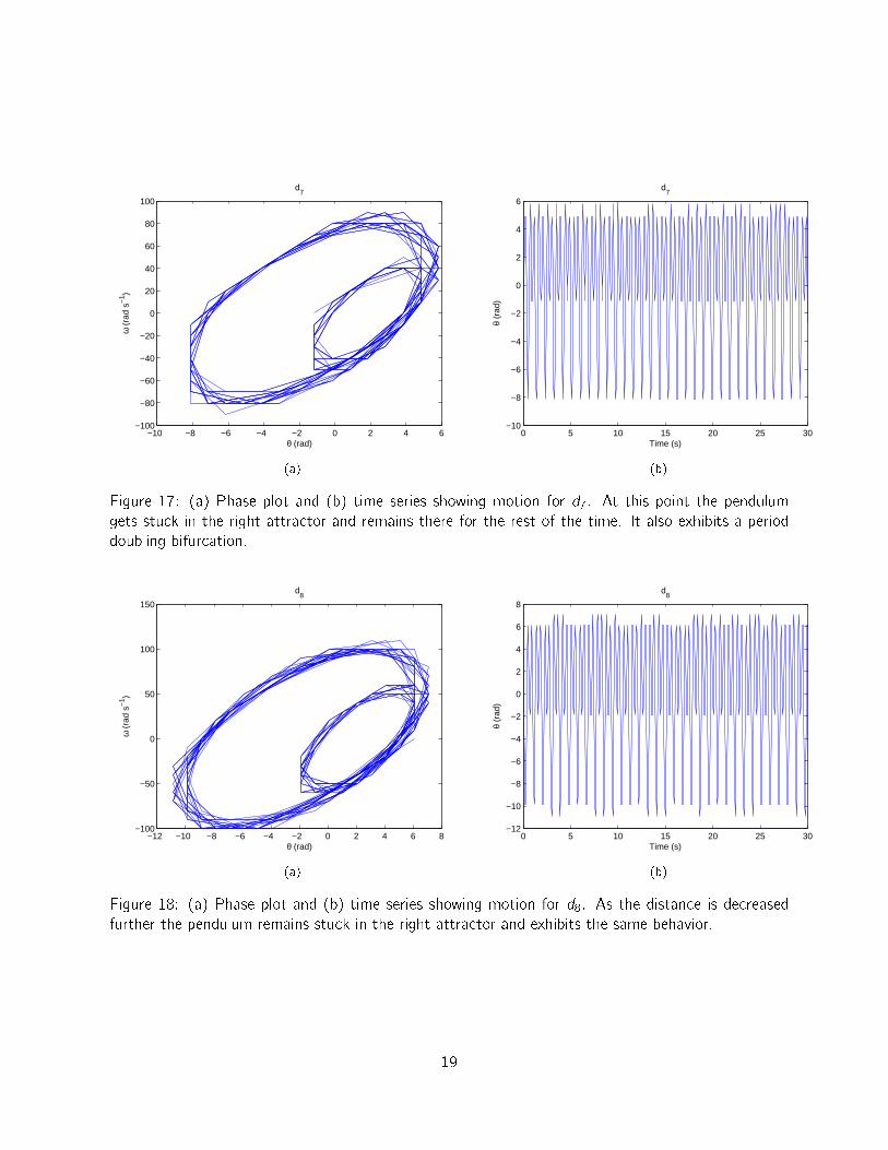
Figure 17: (a) Phase plot and (b) time series showing motion for d7. At this point the pendulum

gets stuck in the right attractor and remains there for the rest of the time. It also exhibits a period

doubling bifurcation.

−12 −10 −8 −6 −4 −2 0 2 4 6 8−100

−50

0

50

100

150

θ (rad)

ω (

rad

s−1 )

d8

(a)

0 5 10 15 20 25 30−12

−10

−8

−6

−4

−2

0

2

4

6

8

d8

Time (s)

θ (r

ad)

(b)

Figure 18: (a) Phase plot and (b) time series showing motion for d8. As the distance is decreased

further the pendulum remains stuck in the right attractor and exhibits the same behavior.

19

4.2.2 Obserivng the Sensitivity of the System by Varying the Initial Conditions

As you might have noticed earlier the pendulum system is extremely sensitive to its initial conditions.

Even if practically you keep everything the same and drive the pendulum, the trajectories on the phase

portrait will never match. This highlights our lack of control over the nonlinear system and its hyper

sensitivity to initial conditions.

To rea�rm our ideas in this regard we will now use our simulation to vary the initial amplitude very

slightly and observe the change in the behavior of the pendulum.

1. Once again, open the pendode1.m �le and select a speci�c d . For example, in our case we

selected the d4 of our simulation results shown previously.

2. The simulation will now be run twice with slightly incongruent initial values. In each case the d

will be kept constant and the initial amplitude will be varied. For example, the amplitudes can

be set at 0:2000 rad and 0:2002 rad in the two runs.

3. Plot the waveform time series and phase portraits for both cases. A set sample results are shown

below.

Question: Do you results agree to our initial hypothesis that the system is extremely sensitive to the

initial conditions?

20

−0.2 −0.15 −0.1 −0.05 0 0.05 0.1 0.15 0.2−0.4

−0.3

−0.2

−0.1

0

0.1

0.2

0.3

0.4

θ (rad)

ω (

rad/

s)

d4, θ

1

(a)

0 20 40 60 80 100 120−0.2

−0.15

−0.1

−0.05

0

0.05

0.1

0.15

0.2

d4, θ

1

θ (r

ad)

Time (s)

(b)

Figure 19

−0.2 −0.15 −0.1 −0.05 0 0.05 0.1 0.15 0.2−0.4

−0.3

−0.2

−0.1

0

0.1

0.2

0.3

ω (

rad

s−1 )

d4,θ

2

θ (rad)

(a)

0 20 40 60 80 100 120−0.2

−0.15

−0.1

−0.05

0

0.05

0.1

0.15

0.2

Time (s)

θ (r

ad)

d4, θ

2

(b)

Figure 20: Figure 19 (a) Phase plot and (b) time series showing periodic motion for d4 and �1. After

exhibiting the pendulum settles into the right attractor. Figure 20 (a) Phase plot and (b) time series

showing periodic motion for d4 and �2 with a slight variation in initial amplitude. The pendulum

exhibits completely chaotic motion throughout. You can see that in the case the pendulum is unable

to decide which attractor it should settle in.

4.3 Observing Amplitude Hysteresis in Pendulum's Behavior

In this last section of the experiment you will carry out a simple exercise. The driving frequency of the

rod will be varied by, as usual, changing the voltage of the power supply. The voltage will be changed

21

from 22:4 to 28:6 V in steps of 0:2 V. At each step you will calculate and record the maximum

amplitude of the signal, obtained in the LABVIEW window. The value of d would be kept constant

at, say 60 cm.

The process will �rst be carried out for increasing voltage (or drive frequency) and then for decreasing

voltage (or drive frequency).

NOTE: Only record the amplitude once the pendulum has reached its steady state at each step.

HINT: You have already noted amplitudes for the increasing frequency part in Section 4:2:1:2. You

only have to note the amplitudes for decreasing frequency.

HINT: Use min() and max() functions in Matlab to calculate the minimum and maximum of the

signal.

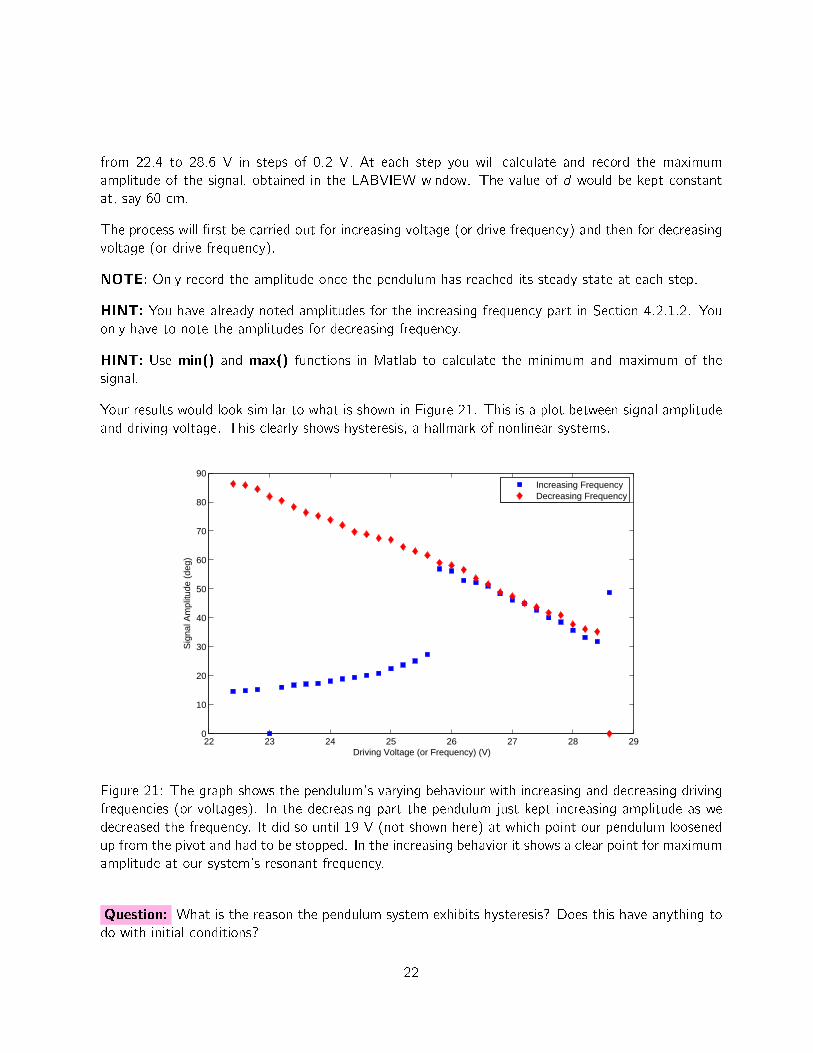
Your results would look similar to what is shown in Figure 21. This is a plot between signal amplitude

and driving voltage. This clearly shows hysteresis, a hallmark of nonlinear systems.

22 23 24 25 26 27 28 290

10

20

30

40

50

60

70

80

90

Driving Voltage (or Frequency) (V)

Sig

nal A

mpl

itude

(de

g)

Increasing FrequencyDecreasing Frequency

Figure 21: The graph shows the pendulum's varying behaviour with increasing and decreasing driving

frequencies (or voltages). In the decreasing part the pendulum just kept increasing amplitude as we

decreased the frequency. It did so until 19 V (not shown here) at which point our pendulum loosened

up from the pivot and had to be stopped. In the increasing behavior it shows a clear point for maximum

amplitude at our system's resonant frequency.

Question: What is the reason the pendulum system exhibits hysteresis? Does this have anything to

do with initial conditions?

22