the macroeconomics of saving, debt and financial development
TRANSCRIPT

The Macroeconomics of
Saving, Debt and Financial Development
Inaugural-Dissertation
zur Erlangung des Grades
Doctor oeconomiae publicae (Dr. oec. publ.)
an der Ludwig-Maximilians-Universität München
2012
vorgelegt von
Sebastian Jauch
Referent: Professor Dr. Gerhard Illing
Korreferent: Professor Ray Rees
Promotionsabschlussberatung: 15. Mai 2013

Berichterstatter: Professor Dr. Gerhard Illing
Professor Ray Rees
Professor Dr. Kai Carstensen
Mündliche Prüfung: 29. April 2013


I
TABLE OF CONTENTS
ACKNOWLEDGMENTS III
ACRONYMS IV
LIST OF FIGURES V
LIST OF TABLES VI
1 INTRODUCTION 1
2 THE GLOBAL SAVING GLUT REVISITED –
CORPORATE SAVINGS AND THE ROLE OF SHARE REPURCHASES
8
2.1 Introduction 9
2.2 Overview of related literature 12
2.3 The corporate saving glut hypothesis – the case of the G7 countries 17
2.4 An empirical analysis of the aggregated corporate saving rate 22
2.4.1 Hypotheses and theory 22
2.4.2 Dataset 25
2.4.3 Descriptive analysis 28
2.4.4 Econometric specification and estimation 29
2.5 Firm-level analysis as robustness check 34
2.6 Conclusion 37
References 40
Appendix 43

II
3 THE EFFECT OF HOUSEHOLD DEBT ON UNEMPLOYMENT –
EVIDENCE FROM EUROPE AND SPANISH PROVINCES
48
3.1 Introduction 49
3.2 Overview of related literature 52
3.3 Household debt and unemployment – a European perspective 54
3.3.1 Data sources 56
3.3.2 Empirical analysis 56
3.4 Household debt and unemployment – the case of Spain 62
3.4.1 Theoretical framework 63
3.4.2 Description of the data 66
3.4.3 Empirical analysis 70
3.4.4 Robustness checks 76
3.4.5 The aggregate effect of household debt on unemployment 80
3.5 Conclusion 82
References 85
Appendix 87
4 FINANCIAL DEVELOPMENT AND INCOME INEQUALITY – A PANEL DATA APPROACH 95
4.1 Introduction 96
4.2 Overview of related literature 97
4.3 Data 101
4.3.1 Description of the dataset 101
4.3.2 Income inequality over time and around the world 104
4.3.3 Financial development over time and around the world 106
4.4 Econometric estimation 107
4.4.1 Basic estimation – comparison with previous research 107
4.4.2 Econometric hurdles 109
4.4.3 Fixed effects estimation 111
4.5 Robustness checks 114
4.6 Conclusion 120
References 122
Appendix 124

III
ACKNOWLEDGMENTS
This dissertation grew over the last three years and would not have been possible without the
support of numerous persons, including family, friends and colleagues. Special gratitude is owed
to my supervisor, Prof. Dr. Gerhard Illing, who not only provided support during my dissertation
and helped me with honest advice early in the process but also convinced me eight years ago to
change my studies from business to economics and thus laid the foundation for this project. I
would like to thank Prof. Ray Rees, for serving as my second supervisor and Prof. Dr. Kai
Carstensen for joining my dissertation committee as the third examiner.
Chapters 3 and 4 of this dissertation are a joint work with Dr. Sebastian Watzka. Sebastian, I
really enjoyed working together with you, and our numerous discussions significantly enhanced
the quality of the papers involved in this dissertation.
I would also like to thank current and former colleagues at the Seminar for Macroeconomics for
helping me in all phases of my dissertation: Dr. Desislava Andreeva, Agnès Bierprigl, Dr. Jin
Cao, Sebastian Missio, Dr. Monique Newiak, Dr. Angelika Sachs, Thomas Siemsen, Dr.
Sebastian Watzka, and my officemate Michael Zabel.
Earlier versions of the three chapters of this dissertation were presented at various workshops and
conferences. I want to thank the participants of several Macro Seminars of our faculty, the
Macroeconometric Workshop at the DIW, Berlin 2011, the National Bank of Serbia Young
Economist Conference, Belgrade 2012, the Macro Money and Finance 44th
annual conference,
Dublin 2012, the conference on Intra-European Imbalances, Global Imbalances, International
Banking, and International Finance, Berlin 2012, and the Workshop on Inequality and
Macroeconomic Performance, Paris 2012, as well as the discussants at the respective
conferences. Ulrich Hendel’s comments on early versions of chapter 2 and 3 were also valuable
in writing this dissertation.
My deepest gratitude goes to my family and close friends, who continuously supported me
beyond the last few years and who gave me exactly the right amount of necessary distraction
from academia.
Sebastian Jauch

IV
ACRONYMS
ATM Automated teller machine
ELF Ethno linguistic fractionalization
EU European Union
FD Financial development
GDP Gross domestic product
GMM Generalized method of moments
IMF International Monetary Fund
INE Instituto Nacional de Éstadistica
IPO Initial public offering
LIS Luxembourg Income Studies
NUTS Nomenclature des unités territoriales statistiques; Nomenclature of territorial units
for statistics
OLS Ordinary least squares
OECD Organisation for Economic Co-operation and Development
PSID Panel Study of Income Dynamics
SIC Standard industrial classification
SWIID Standardized World Income Inequality Database
UN SNA United Nation System of National Accounts
VIF Variance inflation factor
2SLS Two stage least squares

V
LIST OF FIGURES
Figure 2.1 Global gross saving rate including and excluding the United States 10
Figure 2.2 Non-financial corporate sector saving rates in G7 countries 20
Figure A2.1 Piercing the corporate veil? – private and corporate sector saving 47
Figure 3.1 Changes in household sector debt and contribution of consumption
expenditure to GDP growth
57
Figure 3.2 Changes in debt and employment 60
Figure 3.3 Levels of household sector debt and changes in employment 61
Figure 3.4 Spanish household liabilities and unemployment 71
Figure 3.5 Household sector debt and changes in tradable and non-tradable
unemployment
75
Figure A3.1 Changes in household sector debt and contribution of consumption
expenditure to GDP growth
89
Figure A3.2 Household sector debt and tradable employment sectors 90
Figure A3.3 Household sector debt and non-tradable employment sectors 91
Figure A3.4 Debt and unemployment in the Spanish provinces 92
Figure A3.5 Changes in real estate prices and employment in the Spanish provinces 93
Figure A3.6 How a reduction in debt growth affects spending 94
Figure 4.1 Inequality over time 105
Figure 4.2 Financial development over time 106
Figure A4.1 Gross income inequality around the world 131
Figure A4.2 Net income inequality around the world 131
Figure A4.4 Financial development around the world 132
Figure A4.5 Financial development, economic development and income inequality 132

VI
LIST OF TABLES
Table 2.1 Average non-financial corporate saving rates in the G7 countries 18
Table 2.2 Tests of the savings glut hypothesis 18
Table 2.3 Correlation matrix of dependent and independent variables 28
Table 2.4 Regression analysis of the saving rate 31
Table 2.5 Regression analysis of the adjusted saving rate 33
Table 2.6 Firm-level analysis of the corporate saving rate 36
Table A2.1 Non-financial corporate savings rates and share repurchases in OECD-
countries
43
Table A2.2 Share repurchases on a firm level 43
Table A2.3 Overview of variables in dataset 45
Table A2.4 Firm-level correlation matrix of dependent and independent variables 46
Table 3.1 Correlation of household sector debt and unemployment 72
Table 3.2 OLS regression of unemployment on household sector debt 74
Table 3.3 Development of real estate prices, employment and debt in provinces with
high and with low correlations between changes in employment and real
estate prices
78
Table A3.1 Changes in household sector debt and contribution of consumption
expenditure to GDP growth
87
Table A3.2 Economic activities with old and new classifications 88
Table 4.1 Overview of variables and sources 103
Table 4.2 Basic estimation 108
Table 4.3 Fixed effects and 2SLS estimation 112
Table 4.4 Financial development and the Kuznets curve in different income groups 114
Table 4.5 Fixed effects estimation by income group 115
Table 4.6 First difference estimator and lagged variables 118
Table 4.7 Access to finance and the provision of credit 119

VII
Table A4.1 Correlation analysis 1 124
Table A4.2 Correlation analysis 2 125
Table A4.3 First stage regression – financial development 125
Table A4.4 Robustness check with bank deposits as proxy for financial development 126
Table A4.5 Income inequality and financial development by country 127

1
CHAPTER 1
Introduction

Chapter 1: The Macroeconomics of Saving, Debt and Financial Development – Introduction
2
Savings and debt as well as the financial intermediation in between are at the heart of every
economic system. When an economic system is under stress, disrupted or accused of
malfunctioning, it is essential to investigate the core mechanisms and established patterns of this
system. The financial crisis of 2008 and the following recession represent this type of disruption
that provides cause to examine the fundamentals of our economic system. Thus, this dissertation
challenges common wisdom and established theories on private-sector saving and debt as well as
the role of financial intermediation in view of the financial crisis and the following recession in
recent years.
Economic agents who save provide funds to economic agents who take on debt and invest.
Saving and debt are thus inevitably interlinked. The household sector thereby typically has a
surplus of savings over investments and provides these funds to the overall economy, whereas the
corporate sector is believed to invest more than it saves and consequently borrows from the
household sector. These patterns are standard for the institutional sectors in a market-based
economy. There would likely not be any significant private investment without the pooling of
savers’ funds by financial intermediaries. When more funds are pooled in terms of the share of
the population that participates in financial intermediation and in terms of the volume of funds
that are intermediated (e.g., private credit or bank deposits relative to GDP), financial
intermediaries are more effective in conducting their inherent task. The role of these three parties
– savers, borrowers and financial intermediaries – has been and will continue to be at the core of
debates surrounding the financial crisis. In the following three chapters of this dissertation, I
examine these three parties from different perspectives.
All chapters are based on empirical research. I thereby build the regression estimations based on
unique cross-country panel datasets that were partially assembled by me, based on the
aggregation of micro-level data (chapter 2) and datasets that represent a combination of different
existing macro-level datasets (chapters 3 and 4). Common wisdom regarding the three parties and
theories establishing the underlying rationale are challenged in this dissertation. I thereby study
time horizons that are directly linked to the financial crisis (chapters 2 and 3) and long-term
developments occurring over the course of five decades (chapter 4). Chapter 2 investigates the
saving behavior of the corporate sector prior to the financial crisis and over a longer-term
horizon, as the corporate sector was accused of excessive saving. Herein, I challenge the widely
established saving glut hypothesis with a focus on corporate savings. Similar to the allegedly

Chapter 1: The Macroeconomics of Saving, Debt and Financial Development – Introduction
3
unusual behavior of the corporate sector, the behavior of the household sector was also atypical
before the crisis. Households in many Western economies reduced their saving rates prior to the
financial crisis and amassed large amounts of debt. Household sectors consequently became net
borrowers. The effect of this debt and the deleveraging following the financial crisis on the
aggregate demand channel and unemployment are investigated in chapter 3. Chapter 4 is also
motivated by the debates that arose during the course of the financial crisis; this chapter examines
how financial intermediation evolved during the last five decades and how this financial
development affects income inequality.
The contribution of this dissertation to the existing literature is manifold. By incorporating
aggregated firm-level data in a macro-level analysis of corporate savings, chapter 2 shows that
the System of National Accounts ought to be amended by an alternative measure of gross
savings. Furthermore, examining the link between household sector debt and unemployment,
chapter 3 confirms existing empirical research on the United States and Australia for Europe and
particularly Spain and provides a basis for the analysis of the increase in unemployment
following the financial crisis. Chapter 4 tests established theories and rejects older empirical
research on the link between financial development and income inequality and can thus assist
policy makers in understanding this nexus and addressing potential inequality issues. The
timeliness of this dissertation and the relevance of the topics investigated are demonstrated, for
example, by recent coverage of the chapters in The Economist. A special report on the world
economy (“For richer, for poorer”, The Economist (Oct. 13, 2012)) focuses on inequality issues.
Another article discusses academic research regarding the magnitude of [the traditional definition
of] corporate savings (“Dead Money”, The Economist (Nov. 3, 2012)). Furthermore,
unemployment in Spain is at the center of European business news (e.g., “The euro zone isn’t
working”, The Economist (Oct. 31, 2012)). Thus, this dissertation addresses highly topical
macroeconomic issues that are relevant for the public, policymakers and academia. The following
three paragraphs provide a brief motivation and summary of chapters 2, 3 and 4.
Chapter 2
When one analyzes the financial crisis, one reason for the initial burst of the American housing
and subprime bubble can be found in the low interest rate in the years preceding the crisis. This
low interest rate was caused by, among other factors, a “global saving glut”. Ben Bernanke

Chapter 1: The Macroeconomics of Saving, Debt and Financial Development – Introduction
4
postulated this global saving glut (cf. Bernanke (2005)) and thought of it as increasing saving
rates around the world. Subsequently, it was primarily the corporate sector that was blamed for
having excessively saved. In chapter 2, I investigate this global saving glut with regard to the
corporate sector. I find evidence to confirm this hypothesis when using standard national account
figures and when corporate savings consist of retained profits. However, listed companies in
many advanced economies changed their payout behavior in the 1990s and 2000s from dividends
to share repurchases, which are another medium for distributing profits to shareholders. In this
chapter, I aggregate share repurchases from listed companies in 30 OECD countries and correct
the official corporate sector saving rate for aggregated share repurchases. This method leads to
the rejection of the saving glut hypothesis for the corporate sector and shows that the corporate
sector on aggregate did not significantly change its saving behavior relative to GDP in the “global
saving glut” period. The study of the drivers of the corporate saving rate reveals that the most
important determinants of the aggregate corporate saving rate are the lagged saving rate and
profits. The first contribution of this chapter to the literature is that private-sector saving is
normally studied as a whole or with a focus on household saving, but the corporate sector, which
is typically neglected, is at the center of this research. Second, share repurchases have been
investigated in detail in the finance literature, but to the best of my knowledge, there have been
no attempts to aggregate share repurchases for a large number of countries and to study the macro
effects of this changing payout behavior. Third, this research clarifies that the corporate sector
cannot be charged with having excessively high gross savings in its original sense because the
sector did not change its saving behavior significantly relative to the reference period of the
global saving glut.
Chapter 3
As stated, the household sector is typically the net lender of capital to the entire economy.
However, households in the United States and many European countries loaded their balance
sheets with excessive amounts of debt prior to the financial crisis. Realizing that these debt loads
cannot be sustained in the context of the financial crisis, the household sector began a
deleveraging process. The theoretical foundation for this deleveraging is exemplified in the work
of Eggertsson and Krugman (2012). Deleveraging began earlier in the United States than in
Europe, and the effects of this deleveraging on consumption or via the aggregate demand channel
on employment have been subject to studies by Dynan (2012) and Mian and Sufi (2012). Chapter

Chapter 1: The Macroeconomics of Saving, Debt and Financial Development – Introduction
5
3, which is adapted from Jauch and Watzka (2012), closely follows the approach of Mian and
Sufi (2012) and investigates the effects of household debt at the country level in Europe and at a
regional level in Spain. At the European country level, we confirm that increases in household
debt are linked to an increasing contribution of household sector consumption expenditures to
GDP growth, and decreases in household debt are associated with a lower contribution of
household sector consumption expenditures to GDP growth. Furthermore, economies with a high
level of household debt or high increases in household debt exhibit a steeper decline in
employment or increases in unemployment in the economic downturn. To prove that there is a
direct link from household debt via the aggregate demand channel to unemployment, we
investigate Spanish provinces. On a regional level, we can separate local from national demand
shocks. Because household debt is heterogeneous across provinces, provinces that experience a
higher debt level relative to GDP should observe a steeper decline in consumption. This
consumption is linked to local demand and thus local non-tradable sector unemployment.
Differentiating between non-tradable and tradable sectors consequently enables us to confirm the
negative effects of household deleveraging; in our estimation, this deleveraging caused one-third
of the increase in Spanish unemployment from November 2007 to November 2010. This chapter
contributes to the recent field of empirical deleveraging studies by first investigating Europe and
then considering Spain, which is one of the economies that experienced especially high increases
in unemployment. Our European and Spanish findings confirm the results for the United States
and Australia. Thus, chapter 3 provides a fact base for policymakers with regard to the reasons
for the increase in unemployment and for macro-prudential regulators who are concerned with
potential negative implications of household sector debt.
Chapter 4
Although chapter 3 discusses the potential negative effects of household debt, household debt
may also have beneficial effects. In fact, access to finance is viewed as especially positive
because it enables individuals to borrow, to pursue investments in human capital or to found
businesses. Hence, greater debt and easy access to credit can be viewed as financial development
that improves career and business opportunities for all individuals and thus fosters income
equality in a society. This reasoning is key in the theories proposed by Banerjee and Newman
(1993), Galor and Zeira (1993) and Greenwood and Jovanovic (1990). Chapter 4, which is
adapted from Jauch and Watzka (2011), examines this effect of financial development on income

Chapter 1: The Macroeconomics of Saving, Debt and Financial Development – Introduction
6
inequality and tests the aforementioned theories. Existing empirical research that investigates the
financial development income inequality nexus has confirmed the theories that greater financial
development reduces income inequality. We use a broader dataset in terms of countries and a
broader time horizon to estimate the relationship with more appropriate estimation techniques
and a consistent measure of inequality. Using the same OLS approach that was used in previous
research confirms Kuznets curve with respect to the effect of economic development on income
inequality and the lowering effect of financial development on income inequality. However,
when we control for time and country-specific effects, among other factors, and use appropriate
standard errors, the results lead us to reject the Kuznets curve. Furthermore, we find that
increased financial development is followed by a more unequal distribution of income. These
findings are robust to different econometric specifications, different measures of financial
development and different subsamples of the dataset. Although financial development may lead
to more equal opportunities, it does not lead to a more equal outcome regarding income. The
contribution of this chapter to the literature is that, to the best of our knowledge, we use the
largest and most comparable cross-country dataset on income inequality to study the effects of
financial development. This approach enables us to correct for data issues and a lack of coverage
in previous research. The findings are important with regard to policy measures that aim to
reduce income inequality because we show that more finance does not necessarily need to be a
supportive factor, but it rather enables talented individuals to extract higher incomes.

Chapter 1: The Macroeconomics of Saving, Debt and Financial Development – Introduction
7
REFERENCES
Banerjee, A. V. and A.F. Newman (1993): “Occupational Choice and the Process of
Development”. Journal of Political Economy, 101(2): 274–298.
Bernanke, B. (2005): “The Global Saving Glut and the U.S. Current Account Deficit”. Remarks
by Governor Ben S. Bernanke at the Sandridge Lecture, Virginia Association of Economists,
Richmond, Virginia. March 10th
2005.
http://www.federalreserve.gov/boarddocs/speeches/2005/200503102/
Eggertsson, G. B. and P. Krugman (2012): “Debt, Deleveraging, and the Liquidity Trap: A
Fisher-Minsky-Koo approach”. Quarterly Journal of Economics, 127 (3): 1469-1513.
Galor, O., and J. Zeira (1993): “Income Distribution and Macroeconomics”. Review of Economic
Studies, 60(1): 35–52.
Greenwood, J., and B. Jovanovic (1990): “Financial Development, Growth, and the Distribution
of Income”. Journal of Political Economy, 98(5), 1076–1107.
Jauch, S. and S. Watzka (2011): “Financial Development and Income Inequality”. CESifo
Working Paper Series, No. 3687. December 2011.
Jauch, S. and S. Watzka (2012): “The Effect of Household Debt on Aggregate Demand – The
Case of Spain”. CESifo Working Paper Series, No. 3924. August 2012.
The Economist (2012a): “For richer, for poorer”. The Economist. Special report, October 13,
2012: 1-26.
The Economist (2012b): “The eurozone isn’t working”. The Economist. Online edition, October
31, 2012.
The Economist (2012c): “Dead Money”. The Economist. November 3, 2012: 61-62.

8
CHAPTER 2
The Global Saving Glut Revisited –
Corporate Savings and the Role of Share
Repurchases
Abstract
Given that at the time that the “global saving glut” was announced, the global saving rate showed
one of its lowest values in the past three decades, this study seeks to investigate corporate saving
patterns, which are alleged to be significant contributors to the saving glut. I build a unique
dataset with aggregated share repurchases organized on the country level to examine how the
corporate saving rate would actually behave if the System of National Accounts was adjusted for
changing firm payout behaviors, i.e., the increasing distribution of funds to shareholders by
substituting dividends for share repurchases. Using this newly calculated saving rate, I reject the
corporate saving glut hypothesis for the G7 countries. To deepen the understanding of aggregated
corporate saving patterns, I use a large, unique cross-country panel dataset. This shows that
among the examined factors, the lagged saving rate and profitability have the highest impact on
the corporate saving rate.

Chapter 2: The Global Saving Glut Revisited – Corporate Savings and the Role of Share Repurchases
9
2.1 INTRODUCTION
Many different explanations of the recent financial crisis have been suggested. One proposed
cause of this crisis is the global saving glut that contributed to low interest rates, particularly in
the United States, and thereby encouraged risky investments that partially turned out to be bad
ones. The foundations of this argument about the global saving glut were established in March
2005 by Ben Bernanke in his speech addressing “The Global Saving Glut and the U.S. Current
Account Deficit” (cf. Bernanke (2005)), which introduced the notion of a global saving glut.
Bernanke was correct if the global gross saving rate excluding the United States was considered
on a worldwide basis and compared with the gross saving rate of the United States. The United
States was by far the largest importer of capital in the world, whereas the remainder of the world
possessed a savings surplus and exported capital. These large inflows of capital into the United
States helped maintain interest rates at historically low levels. The wide range of literature that
addresses the global imbalances generated by the existence of various exporting or surplus
countries, such as China, Japan and Germany, and one large importer, the United States, relates
to this discussion. A discussion of different explanations for the global imbalances is for example
given by Eichengreen (2006). The saving glut is frequently interpreted in terms of saving
differences between the United States and the rest of the world, primarily Asia (cf. Chinn
(2005)); in Bernanke’s view, these differences are closely linked to global imbalances with
respect to current accounts. However, one can also consider the saving glut from a pure savings
perspective and ask how much capital is provided by the institutional sectors and countries in the
world to maintain fixed capital investments (i.e., to compensate for depreciation) and to increase
the global stock of capital through new investments.
I examine this gross saving rate on a truly global basis and find a different picture than the saving
glut theory would imply. The saving rate1 on a global basis had been trending downward for the
past three decades. In particular, this rate peaked in the late 1970s and declined in long cycles.
The peak of the saving rate cycle in the 1970s is higher than the peak of the saving rate cycle in
the 1980s; similarly, the peak saving rate is higher in the 1980s than in the 1990s, and the peak
saving rate in the 1990s is greater than the peak saving rate in the 2000s. Therefore, the saving
1 Throughout this article “saving rate” and “savings” always refer to gross savings. The concept of gross savings
includes the consumption of fixed capital (depreciation). This consumption represents the difference between gross savings and net savings. The difference between gross savings and net lending primarily represents gross fixed capital formation (investment) (cf. Lequiller and Blades (2006), p.193).

Chapter 2: The Global Saving Glut Revisited – Corporate Savings and the Role of Share Repurchases
10
glut prior to the recent financial crisis is certainly not due to an increase in the global saving rate
above its long-term average, as the global saving rate decreased by approximately 1.2 percentage
points of GDP between the 1970s and the 2000s. Excluding the United States, the global saving
rate reached its peaks of 1977 and 1989 again in 2006. The trend line for this rate indicates an
increase of just 0.01 percentage points per year. At the time of Bernanke’s speech, this rate was
just above its average of the preceding decades and its trend had been stable for the preceding 30
years (cf. figure 2.1).
Figure 2.1
Global gross saving rate including and excluding the United States
Data source: World Bank – World Development Finance.
Decomposing the saving rate in terms of the institutional sectors of the world economy, namely,
households, corporations and governments, as for example done by the McKinsey Global
Institute (2010), reveals the increasing importance of the corporate sector with respect to the
global supply of capital. Government sector savings are of minor importance on a global basis. In
recent decades, household saving rates declined in the developed world, with the steepest
decreases in Italy, Japan, the United Kingdom and the United States, and increased in emerging
markets, such as China and India. In contrast to the developments in the household sector, the
corporate sector increased its share of total savings and its relative saving rate in both developed
and emerging economies. This sector accounts for approximately 2/3 of the supply of capital in
the developed world today. Various entities responded to Bernanke’s speech by arguing that
corporations were leading the global saving glut (cf. The Economist (2005) or Loeys et. al
Global gross saving rate
Years High Low
1970s 23.7 21.4
1980s 22.7 20.9
1990s 22.3 20.6
2000s 22.0 20.3 United States
Global
Global, excl. United States
-0.19 p.a.
-0.04 p.a.
0.01 p.a.
12
14
16
18
20
22
24
26
Pe
rce
nt
of
GD
P
Saving glut period

Chapter 2: The Global Saving Glut Revisited – Corporate Savings and the Role of Share Repurchases
11
(2005)) and the increasing importance of corporate saving was leading to the conventional
wisdom of excessive corporate savings. This point of excess corporate savings was made clear in
analyses by André et al. (2007) and the International Monetary Fund (2006), which indicated that
corporate savings were increasing; in fact, corporate savings surpassed corporate fixed capital
investment in large OECD countries during several years of the early 2000s. Thus, the corporate
sector became a net lender to the economy with high net financial surpluses. It was commonly
assumed that the increase in corporate savings was merely a short-term phenomenon that would
quickly fade (cf. Loeys et al. (2005); International Monetary Fund (2006)).
One consideration that has not been thoroughly accounted for and has traditionally been regarded
as a secondary concern is the impact of share repurchases on corporate savings. A reason for not
including share repurchases in analyses of saving data is that share repurchases are part of
corporate saving according to the official definitions of the System of National Accounts (SNA).2
The magnitude of aggregated share repurchases around the world has not been a focus of
economic research despite the fact that theoretical and empirical explanations for share
repurchases have become available. One contribution of this paper is to close this gap by
aggregating share repurchases on a country level and calculating a new saving rate that reflects
these aspects of corporate saving.
Drivers of corporate gross saving can be determined from the supply and the demand side. The
primary supply-side driver for corporate saving is corporate profits; a certain fraction of these
profits are distributed to a firm’s shareholders, and the remainder is retained within the
corporation, i.e., corporate saving. The primary demand-side driver for corporate saving is the
need for internal capital. Because capital markets are not perfect, firms must utilize internal funds
for a certain fraction of their investments. This requirement creates a demand for corporate
saving. In addition to corporate saving for current investments, other considerations also increase
the demand for corporate saving. Corporate savings can be used to increase corporate cash
holdings, reduce debt, or repurchase shares from shareholders. Cash holdings can be used for
future investment, as insurance against future lending restrictions from capital markets, and as a
buffer that allows a firm to pay out a constant amount of dividends to its shareholders during
2 Share repurchases are incorporated into the financial accounts in the SNA as a source of changes in shareholders’
equity. However, these changes are net figures that also include delistings and IPOs (cf. United Nations’ (2000) Handbook of National Accounting, p. 61ff.).

Chapter 2: The Global Saving Glut Revisited – Corporate Savings and the Role of Share Repurchases
12
times of unstable profits. Debt reductions reduce a firm’s interest expenses and increase its ability
to take on future debts when needed (cf. Achavarya et al. (2005)). Share repurchases are the
fourth demand-side motivation for engaging in corporate saving, as defined by the SNA, although
share repurchases are a substitute to dividends, and the funds that are used for these repurchases
do not remain within the corporation.
Each of these reasons has been studied on its own in theoretical and empirical research; however,
share repurchases are a rather new topic that has not yet been extensively investigated and the
aforementioned studies focus on a firm-level. In this chapter, I present different theories about
corporate savings and then combine the rationales of these theories to estimate the magnitude of
corporate savings on an aggregate level. I calculate an adjusted corporate saving rate by
subtracting share repurchases and compare this adjusted rate with the official corporate saving
rate. I test and reject the hypothesis of a corporate saving glut by aggregating share repurchases
on a national level for the G7 countries. This study contributes to literature on saving behavior by
investigating an institutional sector that is frequently neglected. In particular, the study presented
in this chapter contributes to the extant literature by incorporating share repurchases on a national
level for a large set of countries, which has to the best of my knowledge not been done before.
The chapter is structured as follows. Section 2.2 provides an overview of related literature. In
section 2.3, the hypothesis of a corporate saving glut is tested. Section 2.4 explains the
hypotheses and theories underlying the empirical approach and presents the empirical analysis
with respect to the aggregate corporate saving rate. Section 2.5 repeats the assessments of
corporate savings on the firm level and section 2.6 concludes the chapter.
2.2 OVERVIEW OF RELATED LITERATURE
To the best of my knowledge, there is no significant research addressing the saving behavior of
the corporate sector across a large set of countries. Consequently, in this analysis, I integrate
different streams of literature that relate to this analysis. First, studies addressing macro saving
behavior serve as a starting point for this analysis. Second, finance literature that assesses firm
behavior is used to identify the motivation and theoretical background underlying the derivation
of a regression equation for corporate saving.

Chapter 2: The Global Saving Glut Revisited – Corporate Savings and the Role of Share Repurchases
13
Research on saving rates usually investigates household saving or total private sector saving,
which combines household and corporate saving. In this context, corporate saving includes both
financial and non-financial corporate saving. A main paper on private saving is written by Loayza
et al. (2000), who claim to have built the world’s largest macroeconomic dataset regarding
saving.3 The authors analyze determinants of private saving rates based on a dataset containing
up to 150 countries for a maximum time period of 30 years. They identify the lagged saving rate
as the most important determinant of the saving rate. Although this study and Loayza et al.
(1998) provide a very detailed investigation of private saving, corporate saving alone and the
relationship between household and corporate saving are not thoroughly investigated. Callen and
Thimann (1997) study determinants of household saving in OECD countries. One reason for
choosing the household instead of other institutional sectors is that “most fundamental household
saving, per se, is important because this is the component of saving—rather than public or
corporate saving—that economic theory tells us [the] most about.” (Callen and Thimann 1997, p.
4). However, the limitations of economic theory with respect to corporate saving do not justify
neglecting the study of corporate saving behavior on a macro level, particularly given that the
corporate sector accounts for the majority of the aggregated savings in the world. The common
argument that economists offer for not examining the corporate saving rate in isolation is that
households own corporations and integrate corporate saving decisions into their own saving
decisions. According to this view, which is also known as piercing the corporate veil, the private
saving rate is ceteris paribus constant, and increases in corporate saving are offset by equivalent
decreases in household saving.
Empirical analyses are inconclusive with respect to the extent of this phenomenon. Poterba
(1987) concludes that households only partially pierce the corporate veil, a conclusion that is
supported by Auerbach and Hassett (1991). One argument explaining this result is that the
propensity to consume out of income that is received in the form of dividend payments differs
from the propensity to consume out of a change in wealth if profits are not paid out. These
changes in wealth might also be only temporary. Furthermore, as Poterba (1987) notes, the
ownership structure of shares is highly skewed within the United States. If rich people have a
lower propensity to consume than the poor people and the largest fraction of dividends accrues to
the top 10 percent of the wealth distribution, a change in corporate saving is not mirrored by a
3 The World Saving Database is available at the World Bank website (http://go.worldbank.org/CBSLXPRUN0).

Chapter 2: The Global Saving Glut Revisited – Corporate Savings and the Role of Share Repurchases
14
change in household saving. This is particularly true if the wealth distribution is more skewed
than the income distribution. Moreover, figure A2.1 in the Appendix shows the time trend of
corporate and household savings for selected countries. If households pierced the corporate veil,
changes in one sector should be offset by changes in the other sector. Among the examined
countries, this expectation only holds true for Japan.
Corporate net lending, which reflects corporate savings less corporate investments, is a topic that
has been examined in greater detail than corporate saving (cf. International Monetary Fund
(2006), Loeys et al. (2005) and André et al. (2007)), as corporations in OECD countries exhibited
positive net lending in many years of the previous decade. André et al. (2007) provides a good
descriptive overview of the development of corporate net lending and changes in corporate gross
saving from 2001 to 2005. These authors conclude that most of the increase in net lending is
unlikely to be persistent and that the underlying causes of this increase vary by country. In Japan,
for instance, the observed increase in net lending was motivated by a desire to reduce excessive
debt burdens, whereas in the United Kingdom, this increase was triggered by the increasing
importance and profitability of the financial sector and in Germany, this increase was indicative
of the increased competitiveness of industrial companies.
Few studies addressing the aggregated corporate saving rates of single countries exist. One of
these studies is the investigation of Aron and Muellbauer (2000), who examine corporate saving
in South Africa from 1966 to 1997 and note that corporate saving is “underresearched”. They
estimate a coefficient of 0.5 for the lagged saving rate and conclude that it takes one year to
correct for half of the difference between a particular saving rate and the normal saving rate.
Bayoumi et al. (2010) address Chinese corporate saving, investigating the allegedly excessive
savings of Chinese firms. Based on a comparison of listed Chinese firms with firms from 51 other
countries from 2002 to 2007, Bayoumi et al. (2010) reject the hypothesis that listed Chinese firms
demonstrate a higher saving rate than the global average. Moreover, they explain that high saving
rates in China reflect extensive corporate investment; in fact, this investment caused China to be
the only country in their sample that displayed negative net savings4 over the entire period that
these researchers examined. However, the companies that were investigated reflect only one third
of all enterprise profits in China. The saving rate may thus be comparable on a listed firm level,
4 Bayoumi et al. (2010, p.5) calculate the net saving rate as gross savings/asset - investment/assets. In the SNA
terminology, net savings refers to gross savings less depreciation.

Chapter 2: The Global Saving Glut Revisited – Corporate Savings and the Role of Share Repurchases
15
but the aggregated corporate gross saving rate in China is still among the highest in the world.
Kuijs (2006) takes a different perspective on the Chinese corporate saving rate and argues that it
is among the highest in the world. However, the years used for comparison are 2004 and 2005 for
China and these two years are indeed characterized by high corporate saving rates compared to
previous and following years. Furthermore, the data for the countries of comparison, such as
Japan, Korea and the United States, are from 2002, which are lower than in 2004 or 2005. Kuijs
(2006) explains the high saving rates with the high investment rates that are mainly financed
internally. A potential contradiction between Bayoumi et al. (2010) and Kuijs (2006) can be
explained by the difference between the firm- and country-level analysis. On a firm-level the
saving rates are in line with other countries, because the ratios are built over assets. On an
aggregate level, the rate over GDP is higher than in other countries because the share of capital
intensive industries in the economy is higher for China.
The second block of literature I introduce presents a micro or finance-based view of corporate
savings and firm behavior. André et al. (2007) mention the importance of payout behavior for
gross saving, as gross saving is calculated as profits less dividends. The need to integrate share
repurchases into considerations of corporate saving is based on the increasing relevance of these
behaviors across all of the OECD countries.5
Grullon and Michaely (2002) highlight the
importance of share repurchases in the United States, where share repurchases surpassed
dividends as a method of distributing cash to shareholders for the first time in 1999. They find
evidence for their hypotheses that share repurchases are a substitute for dividends. This
substitution effect is my motivation for treating share repurchases and dividends in a similar
manner by subtracting these repurchases from gross savings. The European Central Bank (2007)
confirms the growing importance of share repurchases in the euro area and claims that excess
profits prior to the financial crisis were the main driver of this habit. Von Eije and Megginson
(2008) investigate patterns of share repurchases in Europe and argue that most of the
observations for the United States can also be found with some time lag in Europe. Based on
these findings, I incorporate share repurchases into my analysis of corporate savings.
There are many reasons for the increasing importance of share repurchases. The rationale behind
share repurchasing programs and a critique of these reasons is not a focus of this chapter.
5 Cf. table A2.1 in the Appendix for an overview of the magnitude of share repurchases in OECD countries.

Chapter 2: The Global Saving Glut Revisited – Corporate Savings and the Role of Share Repurchases
16
However, I nonetheless wish to list the following primary reasons that drive the increasing
popularity of these repurchasing programs. First, executives of listed companies typically receive
shares of the company as an aspect of their compensation. Therefore, companies repurchase their
own shares from the market to ensure that shares are available for distribution to these
executives. Moreover, because the value of the shares executives receive as remuneration is
linked to the share price performance, these executives have an incentive to conduct price nursing
via share repurchase programs. Furthermore, in certain countries, capital gains are taxed
differently than dividends. Therefore, increasing shareholder wealth through repurchases instead
of dividends may provide tax advantages for shareholders. Share repurchases also gained
importance during a period of high corporate profits because share repurchase programs provide
a method for paying out these profits without changing dividends and raising shareholders’
expectations regarding future dividends too much.
The macroeconomic measure of corporate gross savings is reflected by the financial term of
“retained earnings”, i.e., profits after taxes and interest less payouts. One influential reference
that addresses corporate savings is the work of Lintner (1956), who writes about the distribution
of profits among dividends, retained earnings and taxes. Lintner argues that companies smooth
their dividend payments and that dividends therefore depend on both current profits and past
dividends. There are many uses of retained earnings. As discussed above, retained earnings may
be used for share repurchases. Furthermore, companies utilize retained earnings to finance
investments, repay debt, or increase their cash holdings. While the former represents a payout to
shareholders, the latter three purposes for retained earnings have different determinants. As
Myers and Majluf (1984) reveal, internal funds are required to conduct investment; moreover,
their well-known pecking order states that firms prefer internal funds to external funds for
financing investments. Among the many existing empirical studies supporting this pecking order
theory, I want to highlight the survey results of Graham and Harvey (2001). Various researchers,
including Bates et al. (2006), Almeida et al. (2004) and Opler et al. (1999), study reasons for cash
holdings and use firm-level data to assess different time periods in the United States. Through
examinations of different theories and motives, such as the transaction, precautionary, tax and
agency motives, they find that cash holdings increase with idiosyncratic risk, cash flows, growth
opportunities and financing frictions. The work of Acharya et al. (2005) is closely linked to the
studies about cash holdings. However, these researchers exhibit a narrower focus on the

Chapter 2: The Global Saving Glut Revisited – Corporate Savings and the Role of Share Repurchases
17
relationship between cash holdings and the repayment of debt; they find that this relationship
depends on the hedging needs that are created by financial constraints.
The contribution of this study is threefold. First, single- and cross-country analyses of the
corporate sector are scarce. Moreover, the few studies that are available typically examine the
entirety of the corporate sector, including both financial and non-financial corporations. In this
study, I investigate the non-financial corporate sector alone as financial corporations differ in
their behavior from the real economy. Second, share repurchases have attracted increasing
interest in recent years. However, to the best of my knowledge, no attempt has been made to
aggregate share repurchases on a country level for a large set of countries and to combine this
examination with the macro analysis of saving patterns. Third, the adjusted saving rate provides
new insights regarding the saving glut hypothesis.
2.3 THE CORPORATE SAVING GLUT – THE CASE OF THE G7 COUNTRIES
In the time span that Bernanke referred to in his speech about the global saving glut (1996 –
2004), all of the G7 countries exhibited either increased or constant corporate saving rates.
However, this conclusion changes dramatically if the saving rate is adjusted for additional
corporate payouts via share repurchases.6 After this adjustment, the aggregate saving rate of the
G7 countries remains unchanged during the time span of interest, and only Japan and Canada
exhibit a permanent increase in corporate saving rates. A formal test of the saving glut hypothesis
confirms that there was indeed a corporate saving glut in the largest economies of the world for
the years from 1996 to 2004 if the United Nations System of National Accounts (UN SNA)
definition for the corporate saving rate is used. However, this hypothesis must be rejected if a
more appropriate measure of aggregated corporate savings that includes an adjusted rate for share
repurchases is employed (cf. tables 2.1 and 2.2).
6 A detailed description of share repurchases and the adjustment of the saving rate is given in section 2.4.2.

Chapter 2: The Global Saving Glut Revisited – Corporate Savings and the Role of Share Repurchases
18
Table 2.1
Average non-financial corporate saving rates in the G7 countries, as a percentage of GDP
Type of corporate saving rate
Total period (1987-2007)
Before saving glut
(1987-1995)
Saving glut (1996-2004)
Change between the prior period and the saving
glut period
UN SNA definition 10.03 9.46 10.34 +9.3% (0.88 p.p.)
Adjusted 9.35 9.24 9.61 +4.0% (0.37 p.p.)
By the UN SNA definition of corporate saving, during the period of the saving glut, corporations
increased their saving relative to GDP by 9%, or almost a full percentage point. However, after
accounting for share repurchases and employing a saving rate that is adjusted for more modern
firm payout behaviors, this change diminishes to a modest increase of 4% or less than 0.4
percentage points.
A formal test of the hypothesis
against supports this perspective (cf.
table 2.2). Based on the tests that are presented in table 2.2 and the average saving rates shown in
table 2.1, I confirm the hypothesis that the corporate sector did not cause the global saving glut.
Table 2.2
Tests of the saving glut hypothesis (H0: No saving glut)
p-values of median tests
Type of corporate saving rate
G7 countries aggregated
G7 countries pooled
G7 countries aggregated (until 2007)
G7 countries pooled (until 2007)
Original (UN SNA) saving rate 0.001 0.212 0.009 0.036
Adjusted saving rate 0.157 0.373 0.318 0.545
# of observations 18 126 21 147
years - before saving glut (#) 1987-1995 (9) 1987-1995 (63) 1987-1995 (9) 1987-1995 (63)
years - saving glut (#) 1996-2004 (9) 1996-2004 (63) 1996-2004 (9) 1996-2004 (63)
years - after saving glut (#) --- --- 2005-2007 (3) 2005-2007 (21)
# represents the number of observations.
As the saving rate during the saving glut years is not normally distributed, I use a nonparametric
k-sample test on the equality of medians. Using the UN SNA definition, this test strongly rejects

Chapter 2: The Global Saving Glut Revisited – Corporate Savings and the Role of Share Repurchases
19
the null hypothesis that both distributions are drawn from a population with the same median
value for the aggregated saving rate of the G7 countries, thus confirming the saving glut
hypothesis. However, if this test is used to assess the adjusted saving rate, I obtain a p-value of
15.7% and cannot reject the null hypothesis. Pooling the saving rates of all countries provides a
larger number of observations. For the 126 country-year observations the saving glut hypothesis
can also not be rejected. Again, correcting for share repurchases gives a p-value of 37.3% and
strengthens this paper’s hypothesis that the corporate sector did not contribute to a saving glut.
The inclusion of all of the years until the start of the crisis increases the sample size to 147
observations and accounts for the particularly high saving rates that were observed prior to the
crisis. It is particularly apparent for the sample that includes these pre-crisis years that an
examination of standard national account figures produces different conclusions than the results
that are generated from more reasonable economic assumptions underlying the adjusted saving
rate. The hypothesis that all of the saving rates are drawn from a sample with the same median
cannot be rejected for the adjusted corporate saving rate. Thus, if corporate saving measures are
examined in a detailed manner that incorporates an adjustment for all corporate payouts, tests
with four different samples confirm my rejection of the commonly held perspective that a
corporate saving glut occurred prior to the recent financial crisis. Figure 2.2 illustrates the
adjusted and unadjusted saving rates for all G7 countries from 1980 until 2008, providing a
visualization of the differences between these two measures of corporate savings for the by then
largest economies in the world.

Chapter 2: The Global Saving Glut Revisited – Corporate Savings and the Role of Share Repurchases
20
Figure 2.2
Non-financial corporate sector saving rates in G7 countries
The dotted line indicates the saving rate of non-financial corporations, as measured by the SNA. The solid line indicates the adjusted saving rate, which is calculated as the official saving rate less share repurchases.
Figure 2.2(a): Canada, Japan, the United States and the G7 as a whole
Figure 2.2(b): European G7 countries
1) Data prior to 1991 are based on West Germany.
Data source: UN SNA, Bureau of Economic Analyses (BEA), World Saving Data Base, Worldscope.
Canada
United States
Japan
G7
United States change
per year: -0,1325
0
2
4
6
8
10
12
14
16
18
19
80
19
81
19
82
19
83
19
84
19
85
19
86
19
87
19
88
19
89
19
90
19
91
19
92
19
93
19
94
19
95
19
96
19
97
19
98
19
99
20
00
20
01
20
02
20
03
20
04
20
05
20
06
20
07
20
08
Pe
rce
nt
of
GD
P
United Kingdom
France
Germany1
Italy
0
2
4
6
8
10
12
14
16
18
19
80
19
81
19
82
19
83
19
84
19
85
19
86
19
87
19
88
19
89
19
90
19
91
19
92
19
93
19
94
19
95
19
96
19
97
19
98
19
99
20
00
20
01
20
02
20
03
20
04
20
05
20
06
20
07
20
08
Pe
rce
nt
of
GD
P

Chapter 2: The Global Saving Glut Revisited – Corporate Savings and the Role of Share Repurchases
21
By the SNA definitions assumptions, the United States exhibited the same corporate saving rate
in 2008 and 1980, but the adjusted saving rate reveals to us that the yearly decrease in this saving
rate was as high as -.13 percentage points of GDP over the course of almost 30 years. The high
saving rate in Japan can be explained by an extended phase of reducing the debt burdens that
were built up during the Japanese asset bubble in the late 1980s and by the high share of
depreciation caused by a high capital stock. Canada’s increase in corporate saving is linked to a
surge in commodities and the increasing share of the corporate sector in Canada’s GDP.
European corporate saving rates remained in a narrow band during the 1990s and early 2000s but
widened after 2005 based on diverging developments in the European G7 nations with respect to
economic profitability. The corporate saving rates of France and Italy were especially low in the
early 1980s. This phenomenon reflects the high rate of inflation that existed in these countries
during the years in question; these inflation rates discouraged corporate saving because
corporations experienced significant gains from lowering their real debt burden.7
It may be argued that the integration of statistics from more countries, particularly China, could
change the results that are presented above. However, the G7 countries accounted for more than
60% of global GDP in each of the examined years and are therefore a valid proxy for the world
economy. Furthermore, Chinese figures are subject to frequent changes, and the Chinese
economy was not yet of such a big importance during the time frame that Bernanke referenced, as
its share in the world economy was below 5% in 2004. Moreover, Bayoumi et al. (2010) reveal
that listed Chinese corporations do not exhibit a higher saving rate than companies elsewhere.
Chinese aggregated corporate saving rates are for example comparable to the United Kingdom
from 1995 to 2003, falling below the United Kingdom’s rates from 1996 to 1998 and surpassing
it in 2000 and 2001. 2004 is the only year, in which China’s saving rate clearly exceeded its
counterpart in Europe.
These findings alter the understanding of the roles of different sectors prior to the financial crisis
and have significant implications. First, during the alleged saving glut, the corporate sector did
not provide significantly more capital relative to GDP to the global investment market than it did
during the preceding time period. Second, many firms, especially corporations in the United
States, have been heavily decreasing their supply of capital instead of keeping the rate constant.
7 André et al. (2007) calculate inflation adjusted gross saving rates. I refrain from this adjustment but include the
inflation rate as an explanatory variable in the econometric analysis of this study.

Chapter 2: The Global Saving Glut Revisited – Corporate Savings and the Role of Share Repurchases
22
Third, the declining saving rate of American households, which was below 3% of GDP from
2005 to 2007, is moderated and less steep if it is adjusted to account for changes in wealth that
result from corporate share repurchase programs. If households in the top income decile have a
higher propensity to save than the other 90% of households, and because the top 10% also hold
the largest fraction of common stock,8 a large part of the share repurchases can be attributed to
household saving from a wealth perspective. This, however, does not alter the problem of too low
household savings from a distributional perspective, because the majority of households does not
benefit from the share repurchases and the resulting increase in wealth. Fourth, the System of
National Accounts needs to be complemented by other metrics of corporate saving that reflect
changing firm payout behavior. This topic has been extensively studied on a micro level but was
neglected on an aggregated level when looking at savings.
In a next step, I address part of the research needs resulting from the findings presented above by
investigating the determinants of the aggregate corporate saving rate and the changes in these
determinants in the context of an adjusted saving rate.
2.4 AN EMPIRICAL ANALYSIS OF THE AGGREGATE CORPORATE SAVING RATE
2.4.1 Hypotheses and theory
The empirical analysis is based on a selection of theoretical models. There are various theories
that explain demand for internal funds, e.g., investment needs or cash holdings. But those theories
do not cover the entire aspect of corporate savings, so that it becomes necessary to combine the
explanations of several models. A starting point for the empirical analysis in this study is
Lintner’s model of the distribution of corporate income among dividends, retained earnings and
taxes. Following Lintner (1956), I choose profits and the lagged saving rate as main determinants
of the saving rate and supplement these two by further explanatory variables. In his simple
model,
(2.1)
dividends (Divt) are determined by profits (Profitst) and by previous year’s dividends (Divt-1).
Lintner argues that firms actively decide their dividend policy and that savings are therefore
determined by the residual value of firm profits after this distribution of dividends. The rationale
8 Poterba (1987) states that the top decile of the wealth distribution holds 85% of common stock.

Chapter 2: The Global Saving Glut Revisited – Corporate Savings and the Role of Share Repurchases
23
for Lintner’s equation is the belief that because shareholders prefer a stable dividend, managers
only partially adjust dividends to firm profits. Thus, although dividend payout ratios are not held
constant, they are smoothened to avoid raising expectations regarding payouts if exceptionally
high profits are realized in the current year. A constant stream of income via dividends reduces
income uncertainty among shareholders and increases the credibility of firm managers who are
able to provide a consistently positive firm performance.
However, the decision about the amount of dividends to be paid out is at the same time a decision
regarding the amount of earnings that are retained in order to conduct investments, increase cash
holdings, reduce debt or buy back shares. Given an increasing stock turnover rate,9 a reduction of
dividend payout ratios and the increasing share of listed companies that do not pay dividends at
all,10
the argument that savings are merely a residual no longer holds true, and the investigation
of corporate saving patterns is therefore necessary.
Using the distribution of a firm’s profits between dividends and savings, (2.2), I reformulate
Lintner’s model, (2.1), to derive a basic saving equation, (2.3):
(2.2)
(2.3)
As argued above, this saving or dividend-smoothing based on Lintner is insufficient for
estimating a more realistic savings equation. Consequently, to estimate the determinants of
saving, I integrate further theories about the demand for internal funds.
Current investment needs: According to the pecking order theory of Myers and Majluf (1984), a
firm prefers to use internal funds instead of external funds for its investments. Thus, investment
(Inv) is added to the list of explanatory variables. I expect a positive sign for the coefficient of
this variable, given that higher investment is associated with a higher need for financing, and part
of this financing is typically internally funded. The investment variable incorporates current
investments.
9 The stock market turnover rate in the U.S. increased from 0.61 to 3.5 between 1988 and 2009; in the United
Kingdom, this rate increased from 0.75 to 2.67 between 1988 and 2007 (cf. database by Demirgüc-Kunt and Beck (2009)). 10
Eugene F. Fama and Kenneth R. French (2001) report that 2/3 of listed American companies paid cash dividends in 1978 but that only 1/5 of listed American companies paid dividends in 1999.
Chapter 2: The Global Saving Glut Revisited – Corporate Savings and the Role of Share Repurchases
24
Future investment needs: Growth expectations further influence future investments and future
capital requirements. To cope with future financing needs, firms that do not wish to rely on
perfect capital markets must stockpile cash. In firm-level analyses, Tobin’s q is frequently used
as a proxy for future investment opportunities. Because this paper conducts its estimations on a
country level, I use GDP growth (GDPg) as a proxy of future investment needs. Higher levels of
GDP growth should be accompanied by higher saving rates because of the positive investment
outlook and show a positive sign in the analysis. Another indicator is the change in GDP growth
(d_GDPg). Declining growth rates signal decelerating lower future investment demand and
therefore lower capital demand; similarly, increasing growth rates may be regarded as an
indicator of higher capital demand. Thus, the sign of this regressor is also expected to be positive.
Risk and uncertainty: In addition to the influence of investment outlook, corporations also
demonstrate a higher demand for capital when they increase their pile of cash during periods of
higher idiosyncratic risk and higher macro uncertainty. Although idiosyncratic risks are
diminished at the aggregate level in the macro analysis of this study, the inflation rate (cpi) is
used as measure of macro-level uncertainty. The expected positive sign results from a
precautionary motive. The higher the uncertainty, the more funds companies will set aside to
maintain their liquidity. The cash can then be used to smooth dividend payments if profits are
lower than expected and to invest if a more uncertain market outlook leads financial markets to
restrict their provision of funds. However, inflation also produces an opposing effect. Higher
inflation rates increase the costs of holding cash and lower the incentives to save. This negative
effect is reinforced by the impact of inflation on corporate debt. The higher the rate of inflation,
the more debt is inflated away and the lower are the incentives to save. Thus, the overall sign of
the inflation variable is unclear and depends on which of the aforementioned effects prevails.
Changing payout behavior/share repurchases: A further reason to increase savings are share
repurchases (Buybacks), which are added to the model as a regressor. Grullon and Michaely
(2002) show that share repurchases are a substitute for dividends and are conducted out of funds
which would otherwise have been used to pay out dividends. Because share repurchases are
carried out through retained earnings, this method of corporate payout increases the saving rate.
The quantity of share repurchases has been constantly increasing since the 1990s and reached its
peak prior to the financial crisis in 2007. In fact, in 2007, aggregate share repurchases have
reached 4% of GDP in the United States. Share repurchases are an important factor for explaining

Chapter 2: The Global Saving Glut Revisited – Corporate Savings and the Role of Share Repurchases
25
the increase in corporate saving and should therefore exhibit a positive sign in the regression
estimation. Many motivations for share repurchases exist. In addition to the need to pay out funds
to shareholders without increasing dividends and shareholders’ expectations of steady streams of
income, managers also have a high incentive for share repurchases because these transactions
increase the stock price and their remuneration is dependent on the performance of a firm’s stock.
Institutional factors: Additional explanatory power for the demand for internal funds comes from
institutional factors. One of these factors is the depth of financial markets. More advanced
financial markets provide easier access to external financing and therefore involve lower
requirements for internal funds. The reliability of financial markets and the banking system is
crucial for planning the stock of cash that is held by a corporation. If external funds were always
available at a fair rate, there should not be a need to hold on to cash reserves. The ratio of private
credit by deposit money banks and other financial institutions to GDP (finsystem) is a widely
accepted proxy for the development of financial markets.11
Because pooling funds from savers
and channeling these funds to borrowers is the inherent task of financial intermediaries,
increasing credit provision is associated with deeper financial markets. Furthermore, lower
spreads and less expensive risk-adjusted credit terms are indicators of the sophistication of
financial markets and conditions for increasing credit provisions. The depth of financial markets
should have a negative impact on the saving rate since firms need to rely less on internal
financing.
2.4.2 Dataset
Macro-level variables
To test the aforementioned hypotheses regarding the determinants of the saving rate, I use a
unique panel dataset that is based on multiple sources. The main source for all of the savings-
related data that are used in this chapter is the UN SNA.12
The UN SNA provides saving data by
institutional sector, including information on the non-financial corporate sector for 64 countries. I
use a maximum time length of 39 years (1970-2008), depending on data availability. To increase
the number of countries that are included in the assessed data and to derive a more balanced panel
dataset, I append relevant statistics for Australia, Canada, New Zealand and the United States
11
A more detailed description of this proxy can be found in chapter 4. 12
http://data.un.org/Browse.aspx?d=SNA.

Chapter 2: The Global Saving Glut Revisited – Corporate Savings and the Role of Share Repurchases
26
from national sources because the UN SNA data for these nations either do not span the entire
study period or are incomplete with regards to the different variables. The total country sample
comprises 68 countries, including 30 out of the 34 OECD countries.13
The same data sources are
used to obtain additional sector-specific variables, such as gross operating surplus (profits),
consumption of fixed capital (depreciation) and gross fixed capital formation (investment). The
sector variables exclude the financial sector because this sector behaves differently than the real
sector in terms of saving and investment decisions. Furthermore, it is the corporate sector and not
the financial sector that is accused of having excessively saved, whereas financial institutions are
blamed for having accumulated overly high leverage and therewith too much debt. All of the
variables from the UN SNA are obtained as levels but are transformed to ratios over GDP to
exclude size effects, transform the data to stationary series and render the data comparable across
countries.
The World Development Indicators by the World Bank serve as the second source for cross-
country data for the 1970 to 2008 time period. All data on inflation (cpi), GDP growth (GDPg)
and change in GDP growth (d_GDPg) for the 68 countries are based on this database. The data
are again utilized in terms of percentages. Information regarding institutional factors, such as the
depth of financial markets (finsystem), is based on the updated financial institutions database of
Beck and Demirgüc-Kunt (2009), which is available through the World Bank. Beck and
Demirgüc-Kunt provide the ratio of private credit by deposit money banks and other financial
institutions to GDP. This ratio serves as a proxy for the importance of financial intermediation in
a country and the availability of external financing. According to Beck and Demirgüc-Kunt
(2009, p.6), this metric “is a standard indicator of the finance and growth literature”.
Micro-level variables – share repurchases
A major contribution of this paper is the integration of share repurchases into macro-level
research. Because information regarding share repurchases on an aggregate level is not available
through any database, firm-level data regarding share repurchases were collected and aggregated
to derive comparable data on the country level. These firm-level data are based on the
13
Statistics for the OECD countries of Iceland, Israel, Luxembourg and Turkey are not available.

Chapter 2: The Global Saving Glut Revisited – Corporate Savings and the Role of Share Repurchases
27
Worldscope database from Thomson Financial.14
Share repurchases are defined as Purchase of
common and preferred stock based on the firms’ cash flow statements (Worldscope source code
4751). Because the focus of this analysis is on the non-financial sector, I exclude all banks,
insurance companies, holdings and other investment offices with SICs of 6000 to 6499 and 6700
to 6799 from the aggregation of share repurchases. Worldscope claims to cover 95% of global
market capitalization and has full coverage of the United States and Western European markets.
The time series that is covered by Worldscope begins in 1980 and lasts until 2010. As share
repurchases were of minor importance prior to 1980 in the United States15
and nonexistent in
many other countries, I assume the aggregate quantity of share repurchases to be 0.0% of GDP
prior to 1980 for the entire dataset. Worldscope offers data for all of the OECD countries and a
total of 66 countries. As not all countries with information on non-financial saving are covered by
Worldscope, I further reduce the dataset to all of the available OECD countries. This gives a
more homogenous and less unbalanced dataset. More details on share repurchases on an
aggregated level (table A2.1) and on a firm level (table A2.2) are provided in the Appendix.
All of the variables that are used in the analysis are transformed into ratios with respect to GDP,
if applicable. Total levels of saving are not of particular interest to this analysis; I assume that the
size of a single firm affects its options to be active in the financial markets and therefore impacts
its saving decisions but that the size of an economy does not influence its aggregated saving
patterns in a systematic manner. The inclusion of total nominal GDP as a size variable in my
analysis confirms this hypothesis because size did not turn out as significant. The dataset is
unbalanced as not all countries provide the relevant variables for the entire time period.
Unbalanced panel data are problematic if there is a systematic reason for the exclusion or
inclusion of certain country years in the estimation. Following Stock and Watson (2007, p. 351), I
argue that the unbalanced panel is not an impediment in this situation because the length of the
data series for each country is random. There is no relation between saving patterns and the
provision of data for OECD countries when countries like Canada, France and the United States
provide data for the entire time period but Ireland, Switzerland and the United Kingdom do not
14
I am grateful to the Economic Business Data Center of the ifo institute and the Ludwig-Maximilians-Universität München for supporting this research by providing access to Worldscope. 15
Grullon and Michaely (2002) compute the value of repurchases/earnings-ratios for listed American US companies and find an average value of 3% for this proportion between the years 1972 and 1979, with a maximum of 5.4% in 1973. During this period, dividends were an average of 12 times higher than share repurchases, and share repurchases were an average of 0.1% of GDP.

Chapter 2: The Global Saving Glut Revisited – Corporate Savings and the Role of Share Repurchases
28
provide data prior to 2002, 1990 and 1987, respectively. Table A2.1 in the Appendix provides an
overview of the years covered, the maximum and minimum saving rates, and the magnitude of
share repurchases for each country.
2.4.3 Descriptive analysis
To build the dataset for the analysis, I begin with a balanced dataset that addresses a relatively
short time period and includes countries without gaps in the data (N=20, T=10). Increasing the
dataset in width and length alters the correlations of most variables only to a minor extent, which
supports me in increasing the number of observations that are used in this analysis at the cost of
the balanced panel. Two subsets of OECD countries with N=22 and N=30 are used for the
analysis. The larger sample includes Eastern European and Latin American countries. The time
period covers the years from 1979 to 2008 (T=30).16
Table 2.3
Correlation matrix of dependent and independent variables
The adjusted saving rate (saving rate less share repurchases) is labeled Saving_New. The prefix L indicates the first lag of a variable. The number of observations is 565 and covers 30 OECD countries over the years from 1979 to 2008. Correlation coefficients that are insignificant at the 5% level are written in italics.
Variable Saving LSaving Saving_New LSaving_New Buybacks Profits Inv GDPg d_GDPg cpi
Saving 1.000
LSaving 0.899 1.000 Saving_New 0.984 0.876 1.000
LSaving_New 0.893 0.979 0.894 1.000 Buybacks 0.110 0.144 -0.071 0.011 1.000
Profits 0.353 0.305 0.341 0.345 0.073 1.000 Inv 0.372 0.379 0.406 0.418 -0.178 0.258 1.000
GDPg 0.211 0.175 0.221 0.197 -0.051 0.160 0.349 1.000 d_GDPg 0.096 -0.019 0.103 -0.005 -0.038 0.009 -0.060 0.503 1.000
Cpi -0.251 -0.285 -0.225 -0.270 -0.144 0.012 0.172 0.015 -0.092 1.000
Finsystem 0.089 0.129 0.004 0.061 0.468 0.037 -0.076 -0.245 -0.078 -0.400
There is a high correlation between the current and the lagged saving rate for both the original
and the adjusted saving rate. This result indicates the stationarity of the saving rate and shows the
16
In particular, the correlations of Inv and cpi with Saving and Saving_New, respectively, increase by slightly more than 0.1 when the dataset is increased from N=22, T=20 to N=30, T=30. The shift to the larger dataset reduces the correlation of finsystem with Profits, Inv, GDPg and cpi by slightly more than 0.1.

Chapter 2: The Global Saving Glut Revisited – Corporate Savings and the Role of Share Repurchases
29
importance of including the lagged saving rate as a regressor. Share repurchases are only slightly
correlated with the saving rate. While profits, investment and GDP growth are correlated as
expected, inflation is associated with a lower saving rate. Contrary to the hypothesis of inflation
as a proxy for uncertainty and the precautionary motive, higher inflation appears to produce
greater costs from holding internal funds than benefits from insuring against uncertainty; thus,
because an inflationary environment causes the costs of holding cash and the benefits of reducing
the real value of debt to outweigh the value of precautionary motives, inflation is negatively
related to saving. The high correlation of the depth of financial markets with share repurchases
builds on the fact that share repurchases are particularly prevalent in advanced financial markets.
The adjusted saving rate exhibits the same properties as the saving rate except with respect to the
correlations with share repurchases and the depth of financial markets. The latter of these factors
is no longer correlated with the adjusted saving rate, whereas the former factor demonstrates a
negative correlation. All of the variables exhibit relatively high variations across time and across
countries and are therefore suited for panel analyses.17
2.4.4 Econometric specification and estimation
Based on the theories and hypotheses described in section 2.4.1, the model of interest is as
follows:
(2.4)
where is a vector of further explanatory variables as explained above: profits, share
repurchases (Buybacks), inflation (cpi), investment (Inv), GDP growth (GDPg), change in GDP
growth (d_GDPg) and the depth of financial systems (finsystem). Yeardummies are added to
capture time effects that are common for all countries. Econometric issues that need to be
addressed in this type of estimations are nonstationarity, heteroskedasticity and endogeneity.
Nonstationarity: A potential problem of nonstationarity can be neglected as the saving rate is
calculated as ratio over GDP and is bound between 0 and 1. It can consequently be regarded as
stationary.
17
Cf. table A2.3 in the Appendix for a further description of the variables.

Chapter 2: The Global Saving Glut Revisited – Corporate Savings and the Role of Share Repurchases
30
Heteroskedasticity: The Breusch-Pagan/Cook-Weisberg test strongly rejects the hypothesis of
homoskedasticity so that I use robust standard errors in all estimations to deal with
heteroskedasticity.
Endogeneity: The issue of endogeneity is more severe: The econometric specification with a
lagged dependent variable combined with the characteristics of this macro-level dataset (rather
small N and large T) is not ideal for econometric analyses. There are country-inherent
characteristics, like firm structure, sector mix and institutional factors that are not covered by the
regressors in the estimation equation. A fixed effects model is a good choice to allow for this
obstacle. Fixed effects models require exogenous regressors and thus do not work properly in
combination with a lagged dependent variable as the lagged dependent variable is vulnerable to
endogeneity and therefore violates an OLS assumption. This endogeneity causes a bias that
increases for greater correlation coefficients. However, because the bias caused by the lagged
dependent variable diminishes with increasing time periods, fixed effects models can still be used
under certain circumstances. As shown by Alvarez and Arellano (2003), a fixed effects model
can be used if one accepts a bias of the magnitude 1/T. Because panel data estimation methods
are mostly developed for micro data (N→ ∞ and small T), the asymptotic properties of those
estimators do not fit macro panels (moderate N and moderate to large T) very well. I still use the
fixed effects model as the bias diminishes to 6% as T → 18.18
This has to be kept in mind when
interpreting the coefficients. In his description of the Arellano-Bond and Blundell-Bond GMM
estimators, which are typically used for dynamic panel data, Roodman (2009) states that “If T is
large, dynamic panel bias becomes insignificant and a more straightforward fixed effects
estimator works”. To compare the fixed effects model with a GMM model, I use the Arellano-
Bond estimator. Both the Arellano-Bond and Blundel-Bond estimators require the number of
instruments to be smaller than the number of groups. Overfitting a model by including too many
instruments brings those GMM estimators closer to an OLS estimator, which is acceptable if the
large number of instruments results from a large number of years (cf. Alvarez and Arellano,
2003). Overfitting is apparent for this panel dataset with 30 OECD countries and more than 20
years of observations, given that the number of instruments is increasing quadratically in T for a
standard GMM setting (cf. David Roodman, 2007). As Alvarez and Arellano (2003) argue, the
18
Although T=30, due to the unbalanced nature of the dataset, the average number of years for N=22 is 20, and the average number of years for N=30 is 18.

Chapter 2: The Global Saving Glut Revisited – Corporate Savings and the Role of Share Repurchases
31
convergence to an OLS estimator is desirable if it is caused by a large T because the endogeneity
bias is reduced by the number of time periods. Therefore I choose the Arellano-Bond estimator,
albeit with the realization that this estimator will generate a bias that in this case approaches 1/N
(cf. Alvarez and Arellano, 2003). Both regressions produce similar results, as shown in table 2.4.
Table 2.4
Regression analysis of the saving rate
I estimate different models to examine the impact of the independent variables on the saving rate for the time horizon and country set covered in these data. T=30 and represents the years from 1979 to 2008. N=30 represent all OECD countries except for Iceland, Israel, Luxemburg and Turkey. N=22 is a further reduced subset of OECD countries that excludes all Eastern European and Latin American OECD countries. The Arellano-Bond model is estimated with the dynamic panel data command xtdpd. LSaving, Buybacks and Profits are treated as endogenous, and GMM-type instruments are used. Robust standard errors are used in all estimations.
Fixed effects model
Arellano-Bond
Non-dynamic
Dynamic
Dynamic
Variable
N = 22 N = 30
N = 22 N = 30
N = 22 N = 30
LSaving
- -
.6808*** .6195***
.6711*** .6264***
Buybacks
.2128 .3691
.0741 .2071
.0820 .1966
Profits
.2545* .3454**
.1211** .1731**
.1276** .1723**
Inv
.0007 .1520
-.0547 .0063
-.0427 .0083
cpi
-.0007 -.0008
-.0001 .0001
-.0003 .0000
GDPg
.0025* .0009
.0005 -.0003
.0005 -.0004
d_GDPg
-.0001 .0003
.0018*** .0014***
.0018*** .0014***
finsystem
-.0164 ** -.0159 *
-.0064*** -.0069**
-.0063 *** -.0065**
constant .0775*** .0183 .0283** .0060 .0261** .0109
# of observations
475 588
460 565
460 565
within-R²
0.47 0.48
0.73 0.68 between-R²
0.07 0.13
0.95 0.77
overall-R² 0.19 0.22 0.86 0.76
Test for 2nd-order auto-correlation 0.05 0.09
***, **, * denote statistical significance levels at 1%, 5% and 10%.
Before interpreting these results, I refer to a study by Judson and Owen (1999) who show that
GMM produces an underestimation of coefficients, whereas an OLS estimator overestimates the
coefficient of the lagged dependent variable and underestimates the coefficients of the other
regressors. Furthermore, the inclusion of a lagged dependent variable suppresses the explanatory
power of the other regressors. Therefore I estimate a model without the lagged saving rate for
comparison. The lagged dependent variable can be regarded as conveying the long-run effects of

Chapter 2: The Global Saving Glut Revisited – Corporate Savings and the Role of Share Repurchases
32
the other regressors and showing the persistence of the saving rate, independent from the most
recent macroeconomic developments.
Including the lagged saving rate in the regression increases the R² values of the N=22 and N=30
estimations from .19 and .22, respectively, to .86 and .76, respectively. The high coefficient of
LSaving indicates that approximately two thirds of the saving rate is predicted by factors from
previous years. The current saving rate determines 24% of the saving rate in three years for the
larger sample of countries (32% for the smaller sample of countries). Profits also have a large
influence with 17% and 12%, for the N=30 and N=22 estimations, respectively. When the ratio of
profits to GDP increases by 1 percentage point the saving rate increases by .17 percentage points.
Not taking previous years saving into account would double the impact of profits on the saving
rate. Changes in the rate of GDP growth do have a significant but only minor influence.
Finsystem, the proxy for the depth of the financial system and the availability of credit, is as
expected and has a negative and significant impact. Every increase of 10 percentage points in the
ratio of private credit to GDP decreases the corporate saving rate by .06 percentage points. Most
surprisingly, share repurchases as well as investment, both key uses of internal funds, do not
influence the magnitude of corporate saving on an aggregated basis in the dynamic and non-
dynamic models. On an aggregate level, the corporate sector’s capital supply to the economy is
independent of its actual capital needs but reacts to institutional settings, operating surpluses and
changes in the rate of GDP growth. The main difference of including Eastern European and Latin
American countries in the analysis is a lower impact of the lagged saving rate and a higher
influence of profits, showing that these countries exhibit less stable saving rates. The results of
the Arellano-Bond approach for the N=22 country sample show a high level of 2nd
-order
autocorrelation that can just be rejected at the 5 percent level. This means that the use of lagged
instruments is not valid and that we cannot properly interpret the estimation results.
Table 2.4 presents the effects for the non-financial corporate saving rate as measured by the SNA.
In a second step I amend the definition of savings in order to derive a more accurate description
of savings. Savings in this logic are all funds that are kept within a firm to fulfill an inherent task,
i.e., to invest, to prepare for uncertainty by increasing cash holdings or to decrease outstanding
debt. The derivation of this adjusted saving is described in the data section in detail. Nominal
share repurchases are aggregated per year on the country-level, then a ratio of the aggregated
share repurchases over GDP is build and this is subtracted from the standard corporate sector

Chapter 2: The Global Saving Glut Revisited – Corporate Savings and the Role of Share Repurchases
33
saving rate to derive the adjusted saving rate. The estimation for this adjusted saving rate is
shown in table 2.5.
Table 2.5
Regression analysis of the adjusted saving rate
I repeat the regressions that are presented in table 2.4 but use the adjusted saving rate Saving_New as the dependent variable. The GMM-type instruments in the Arellano-Bond model are LSaving_New and Profits. Robust standard errors are used in all estimations.
Fixed effects model Arellano-Bond
Non-dynamic
Dynamic
Dynamic
Variable
N = 22 N = 30
N = 22 N = 30
N = 22 N = 30
LSaving_New
- -
.6507*** .5977***
.6335*** .5951***
Profits
.2800* .3616***
.1320*** .1833***
.1405** .1820**
Inv
.0437 .1690***
-.0451 .0142
-.0399 .0181
cpi
-.0008 -.0009***
-.0002 .0001
.0003 .00020
GDPg
.0021** .0007
.0003 -.0004
.0004 -.0005
d_GDPg
.0001 .0004
.0018*** .0014***
.0018*** .0015***
finsystem
-.0189 ** -.0179 ***
-.0077** -.0078**
-.0072** -.0073**
constant .0646** .0163 .0230*** .0067 .0277*** .0132
# of observations
475 588
460 565
460 565
within-R²
0.42 0.45
0.68 0.65 between-R²
0.12 0.16
0.87 0.72
overall-R² 0.20 0.22 0.82 0.73
Test for 2nd-order autocorrelation 0.10 0.14
***, **, * denote statistical significance levels at 1%, 5% and 10%.
The regression analysis for the adjusted saving rate produce similar results as the regression
analysis of the original saving rate. All regressors in the models with N=30 keep their signs and
the only regressors that change their signs in the N=22 models are insignificant. The same
regressors are significant in both sets of dynamic analysis, albeit with slight changes in the t-
values. Differences arise in the coefficients. Compared to the original saving rate, the impact of
the lagged saving rate decreases and profits and the depth of the financial system are of higher
importance. Contrary to my expectations, the exclusion of share repurchases, which are regarded
as a measure to distribute additional profits to shareholders, does not smooth the saving rate but
instead reduces the influence of the previous year’s saving rate and increases the impact of the

Chapter 2: The Global Saving Glut Revisited – Corporate Savings and the Role of Share Repurchases
34
more volatile profits. However, the magnitude of the differences between the coefficients is
small.
The only specification that has different significant independent variables for the original and
adjusted saving rate is the non-dynamic model in the case of 30 countries. In the estimation for
the adjusted saving rate, investment and inflation turn out to be significant. This result is in line
with the expectations. When I measure the saving rate as savings that are indeed maintained
within the corporate sector, investment is highly significant and its impact is approximately 50%
lower than the impact of profits.19
This result gives further support to amend the saving rate
definition of the SNA for share repurchases, since one would expect that investment has to have
an impact on retained earnings of the corporate sector.
2.5 FIRM-LEVEL ANALYSIS AS ROBUSTNESS CHECK
Investigating the aggregate saving rate does not completely reveal the behavior at the firm level.
To study which part of firm level behavior disappears by looking at the aggregate saving rate, the
estimation of the macro level is repeated on a firm level for selected countries as a robustness
check. All of the macro variables are from the sources that are described in section 2.4.2. The
firm-level data are again based on Worldscope and cover the three largest European economies,
namely, France, Germany and the United Kingdom. The examined time period is 1980 to 2010,
and the number of companies that are examined is 4399. I proceed as in section 2.4, and exclude
companies with SIC 6000 to 6499 and 6700 to 6799. The regression equation is as follows:
(2.5)
where is a vector of macro variables (inflation (cpi), GDP-growth (GDPg), change in GDP-
growth (d_GDPg) and the depth of financial systems (finsystem)), and is a set of firm-level
19
Extending the dataset to the maximum number of countries with information on share repurchases and aggregate corporate saving rates yields a dataset with 60 countries and approximately 900 country-year observations. This broader dataset has a similar coefficient for the lagged saving rates (both, the original and the adjusted saving rate) as the OECD countries. However, profits are insignificant, investment is significant and the coefficient of finsystem doubles. The implication of this result backs the theories that corporations need to rely more on internal financing in countries with less developed financial systems. But I abstain from elaborating on these results because the inclusion of the less developed countries reduces the average number of observations per country, which harms our econometric approach.

Chapter 2: The Global Saving Glut Revisited – Corporate Savings and the Role of Share Repurchases
35
variables (profits/assets, capex/assets20
, share buybacks/assets) instead of country-level variables.
Yeardummy is again added to capture time effects. Following Bayoumi et al. (2010), all of the
firm-level ratios are calculated over assets and not profits because profits can be negative,
hindering proper estimation procedures. Profits are calculated by adding net income (Worldscope
source code 01551), dividends (#04551) and depreciation (#01151). Capex (#04601) and assets
(#02999) are taken as provided by Worldscope. Share buybacks (#04751) are set to 0 for a firm if
no value for these buybacks is reported in Worldscope. The number of observations is reduced by
building the ratios, excluding the top and bottom 1‰ of the saving/assets and capex/assets ratios
and integrating the macro variables into the estimation that are not available for the whole time
span from 1980 to 2010 for the three countries. Depending on the estimation process, the sample
used comprises approximately 1,600 firms and 14,800 to 16,000 firm-year observations.
Combining firm-level and macro variables produces certain drawbacks. Firm-level data are
restricted to listed firms and do not represent the entire economy. Furthermore, listed firms are
likely to be multinationals. Thus, data for these firms are likely to include profits and investments
from foreign activities and therefore will not perfectly match the respective macro variables that
are bound to a country’s borders. This explains part of the deviation from the results that are
presented in tables 2.4 and 2.5. Furthermore, there is a higher variation in firm data than in macro
data. The aggregated data are likely to be stickier due to the averaging effect over the whole
economy. Table 2.6 presents the results for the firm-level estimations.
20
Capex stands for capital expenditure, i.e., investment.

Chapter 2: The Global Saving Glut Revisited – Corporate Savings and the Role of Share Repurchases
36
Table 2.6
Firm-level analysis of the corporate saving rate
Compared with the models that are presented in tables 2.4 and 2.5, the firm-related variables are constructed as ratios over assets. All of the models are estimated with xtdpd because a fixed effects model would lead to high biases due to the low value of T for these models. LSaving, LSaving_New, Buybacks/Assets and Profits/Assets are treated as GMM-type instruments. Robust standard errors are used in all estimations.
UN SNA saving rate definition
Adjusted saving rate
Variable
Aggregated model Including size var.
Aggregated model Including size var.
Firm
-lev
el
LSaving
.0525 .0517 LSaving_New
.0516 .0413
Buybacks/Assets
-.0307 .0099 Profits/Assets
.7102*** .5930***
.7347*** .6709***
Capex/Assets
.0405** .0441**
.0534*** .0558***
Log_Assets
-.0241***
-.0198**
Mac
ro-
leve
l
cpi
.0017 .0006
.0011 .0002
GDPg
.0009 .0016
.0009 .0012
d_GDPg
.0026 .0010
.0023 .0011
Finsystem
.0028 .0202
.0082 .0223
Constant .0304** .4732*** .0170 .3837**
# of observations
15,990 15,990
14,842 14,842 # of groups
1,607 1,607
1,550 1,550
Test for 2nd-order autocorrelation 0.33 0.41 0.23 0.22
***, **, * denote statistical significance levels at 1%, 5% and 10%.
The profit and investment ratios are the significant explanatory variables of the saving rate on a
firm level. Compared with the macro level, the lagged dependent variable does not significantly
influence the current saving rate. These findings are in line with the conclusions of the finance
literature presented in section 2.2 of this chapter. Approximately two thirds of every additional
unit of profit are retained within the firm. Higher investment and capital demand lead to higher
savings, but the effect of these factors (4%) is relatively low. In highly developed financial
markets, such as the countries in this sample, external financing should be available at fair rates;
this condition explains the low coefficient of the investment variable. The results change only
marginally if the adjusted saving rate is considered. The impact of profits is slightly lower and
capital expenditures are slightly more important. The largest and most surprising difference
between the two measures of saving is the coefficient of a firm’s size. Larger firms should
experience easier access to capital markets and bank lending. We should therefore observe a
significant negative coefficient for log_assets because larger firms should experience less

Chapter 2: The Global Saving Glut Revisited – Corporate Savings and the Role of Share Repurchases
37
financing frictions and thus experience a lower requirement to save. However, this link is only
apparent for the original saving rate and disappears if the saving rate is adjusted for share
repurchases. Moreover, none of the included macro variables significantly influences a firm’s
saving rate. A firm’s saving decision is based on its own profits and investment needs, but does
not respond to inflation or overall GDP growth. This might occur on the one hand because firms
that are included in the dataset are largely multinationals that are less dependent on the national
economic environment compared to smaller domestic companies and on the other hand because
these firms may be more dependent on sector-specific dynamics than on the status of the overall
economy of their home country.
2.6 CONCLUSION
This study confirms the hypothesis of a global saving glut, although this confirmation only
applies if corporate savings are measured through the methodology of the System of National
Accounts. The investigation of corporate saving in this study show that in the G7 countries
between 1996 and 2004, an average of 7 percent of corporate savings were not retained within the
corporate sector to conduct investment, increase cash holdings or reduce debt; instead, these
savings were distributed to shareholders via share repurchases. In 2007, the share of corporate
savings that was distributed to shareholders via share buybacks even reached 23% for the G7
countries. Adjusting the saving rate for this changing payout behavior consequently leads to the
rejection of the hypothesis that the corporate sector experienced a saving glut between 1996 and
2004. The reasons for different payout behaviors (dividends vs. share repurchases) are not
investigated in this study, but I demonstrate that share repurchases gained importance on an
aggregate level in OECD countries and were responsible for a corporate saving glut with regards
to the official aggregated corporate saving rate. Declining household saving rates in advanced
economies should also be regarded under this aspect. There is no income flow to households, but
households benefit from increased wealth by share repurchase programs. However, this increased
wealth may be temporary in nature and furthermore benefits only the small fraction of the
population who owns shares. Adjustments for payout behavior do not generally alter the
significance of the factors that determine the corporate saving rate both on an aggregate level and
on a firm level because they produce only marginal changes in the coefficients of these factors.

Chapter 2: The Global Saving Glut Revisited – Corporate Savings and the Role of Share Repurchases
38
The non-dynamic specification of the adjusted saving rate for the case of N=30 shows the only
divergence from the results of the traditional saving rate. Yet, this change is important since it
shows that once the saving rate really measures retained earnings, investment needs turn out to be
a significant determinant of corporate savings. While share repurchases have large aggregate
effects and may affect the behavior of managers who nurse the share price by share repurchase
programs, the effect on the determinants of the saving rate is limited.
Aggregate corporate saving rates are most dependent on previous years’ saving rates; the next
most important determinants of corporate saving rates are profits, changes in the rate of GDP
growth and the depth of the financial system. If policy makers want to change the capital supply
of the corporate sector, they need to keep in mind the following two observations: First, the
aggregate saving rate is sticky, and adjustments to this rate occur over several years. Second,
profits are the most important lever for affecting these rates, a conclusion that is confirmed by the
micro-level analysis of this study. In OECD countries, efforts to encourage or discourage
investment produce at maximum slight effects on corporate propensities to save. To counter a
potential saving glut, politicians should foster their nation’s financial systems, as the depth of
financial systems produces a significant and negative effect on corporate savings, but foremost it
is the profit share of the corporate sector that has the highest impact on corporate savings.
Furthermore, the next revision of the System of National Accounts should consider new
classifications for corporate payout behavior. Share repurchases that even surpass the volume of
dividend payments for some country-year observations merit different treatment than normal
corporate savings and should be regarded as a payout to shareholders not only in the finance
literature but also in other economic contexts.
The contribution of this paper to the literature is that to the best of my knowledge, it is the first
cross-country analysis of the corporate saving behavior of the non-financial corporate sector for a
large set of countries. Furthermore, this study is the first to aggregate share repurchases on a
country level for several countries and to include this in the study of corporate savings. The
saving glut hypothesis is frequently adopted by the media, and this paper establishes certain facts
that supplement the common beliefs about this hypothesis. The field of share repurchases,
corporate savings and the saving glut offers a wide range of interesting topics that should be
addressed by future studies. Among these is the effect of share repurchases on current account
imbalances or how a reversion towards more dividend payments would affect household saving.

Chapter 2: The Global Saving Glut Revisited – Corporate Savings and the Role of Share Repurchases
39
The latter issue is particularly interesting because of the contrast between highly volatile stock
market performances and the anticipated stability of the direct flow of money through dividends.

Chapter 2: The Global Saving Glut Revisited – Corporate Savings and the Role of Share Repurchases
40
REFERENCES
Acharya, V. V., Almeida, H. and M. Campello (2007): “Is cash negative debt? A hedging
perspective on corporate financial policies”. Journal of Financial Intermediation, 16 (4):
515–554.
Almeida, H., Campello, M. and M. S. Weisbach (2004): “The Cash Flow Sensitivity of Cash”.
Journal of Finance, 59(4): 1777–804.
Alvarez, J. and M. Arellano (2003): “The Time Series and Cross-Section Asymptotics of
Dynamic Panel Data Estimators”. Econometrica, 71(4): 1121–59.
André C., Guichard, S., Kennedy, M. and D. Turner (2007): “Corporate Net Lending: A Review
of Recent Trends”. OECD Economics Department Working Papers 583.
Aron, J. and J. Muellbauer (2000): “Personal and Corporate Saving in South Africa”. World Bank
Economic Review, 14(3): 509–44.
Auerbach, A. J. and K. Hassett (1991): “Corporate Savings and Shareholder Consumption”.
In: B. Douglas Bernheim and John B. Shoven (Eds.) National Saving and Economic
Performance: National Bureau of Economic Research, Inc (NBER Books): 75–102.
Bates, T. W., Kahle, K.M. and R. M. Stulz (2009): “Why Do U.S. Firms Hold So Much More
Cash than They Used To?”. The Journal of Finance 64 (5): 1985-2021.
Bayoumi, T., Tong, H. and S-J. Wei (2013): “The Chinese Corporate Savings Puzzle: A Firm-
level Cross-country Perspective”. In: Joseph Fan and Randall Morck (Eds.): Capitalizing
China. University of Chicago Press: 283–308.
Bernanke, B. (2005): “The Global Saving Glut and the U.S. Current Account Deficit”. Remarks
by Governor Ben S. Bernanke at the Sandridge Lecture, Virginia Association of Economists,
Richmond, Virginia. March 10th 2005.
http://www.federalreserve.gov/boarddocs/speeches/2005/200503102/
Beck, T. and A. Demirgüç-Kunt (2009): “Financial Institutions and Markets Across Countries
and over Time: Data and Analysis”. World Bank Policy Research Working Paper, No. 4943.
Callen, T. and C. Thimann (1997): “Empirical Determinants of Household Saving - Evidence
from OECD Countries”. IMF Working Papers, 97/181.

Chapter 2: The Global Saving Glut Revisited – Corporate Savings and the Role of Share Repurchases
41
Chinn, M. D. and H. Ito (2007): “Current account balances, financial development and
institutions: Assaying the world “saving glut””. Journal of International Money and Finance,
26 (4): 546–569.
Eichengreen, B. (2006): “The Blind Men and the Elephant”. Issues in Economic Policy, 2006 (1):
1-24.
Eije, H. and W. L. Megginson (2008): “Dividends and share repurchases in the European Union”.
Journal of Financial Economics, 89(2): 347–74.
European Central Bank (2007): “Share Buybacks in the Euro Area”. Monthly Bulletin May 2007:
103-11.
Fama, E. F. and K. R. French (2001): “Disappearing dividends: changing firm characteristics or
lower propensity to pay?” Journal of Financial Economics, 60(1): 3–43.
Graham, J. R. and C. R. Harvey (2001): “The theory and practice of corporate finance: evidence
from the field”. Journal of Financial Economics, 60(2-3): 187–243.
Grullon, G. and R. Michaely (2002): “Dividends, Share Repurchases, and the Substitution
Hypothesis”. Journal of Finance, 57(4): 1649–84.
International Monetary Fund (2006): “Awash with cash: Why are corporate savings so high”.
World Economic Outlook. April 2006.
Loeys, J., Mackie, D., Meggyesi, P. and N. Panigirtzoglou (2005): “Corporates are driving the
global saving glut”. Global Issues. JP Morgan Research. 2005, June 24th.
http://atriumadvisors.com/biarritz/bg/documents/Global%20Savings%20Glut.pdf
Judson, R. A. and A. L. Owen (1999): “Estimating dynamic panel data models: a guide for
macroeconomists”. Economics Letters, 65(1): 9–15.
Kuijs, L. (2006): “How Will China’s Saving-Investment Balance Evolve?”. World Bank Policy
Research Working Paper, No. 3958. July 2006.
Lequiller, F. and D. Blades (2006): “Understanding National Accounts”. OECD Publishing.
Lintner, J. (1956): “Distribution of Incomes of Corporations Among Dividends, Retained
Earnings, and Taxes”. The American Economic Review, 46(2): 97–113.

Chapter 2: The Global Saving Glut Revisited – Corporate Savings and the Role of Share Repurchases
42
Loayza, N., López, H., Schmidt-Hebbel, K. and L. Servén (1998): “Saving in the World: Stylized
Facts”. Working Paper.
http://siteresources.worldbank.org/INTMACRO/Resources/styletxt.pdf
Loayza, N., Schmidt-Hebbel, K. and L. Servén (2000): “What Drives Private Saving Across the
World?” Review of Economics and Statistics, 82(2): 165–81.
McKinsey Global Institute (2010): “Farewell to cheap capital? The implications of long-term
shifts in global investment and saving”. December 2010.
http://www.mckinsey.com/insights/mgi/research/financial_markets/farewell_cheap_capital
Myers, S. C. and N. S. Majluf (1984): “Corporate financing and investment decisions when firms
have information that investors do not have”. Journal of Financial Economics, 13 (2):187–
221.
Opler, T., Pinkowitz, L., Stulz, R. and R. Williamson (1999): “The determinants and implications
of corporate cash holdings”. Journal of Financial Economics, 52(1): 3–46.
Poterba, J. M. (1987): “Tax Policy and Corporate Saving”. Brookings Papers on Economic
Activity, 1987 (2): 455–516.
Roodman, D. (2007): “A Note on the Theme of Too Many Instruments”. Center for Global
Development. Working Paper No. 125.
http://www.cgdev.org/content/publications/detail/14256
Roodman, D. (2009): “How to do xtabond2: An introduction to difference and system GMM in
Stata”. Stata Journal, 9(1): 86–136.
Stock, J. H. and M. W. Watson (2003): Introduction to Econometrics. Addison-Wesley, Boston.
The Economist (2005): “The corporate savings glut”. The Economist. July 7th
, 2005.
United Nations (2000): “Links Between Business Accounting and National Accounting”. Studies
in Methods. Handbook of National Accounting. United Nations, New York, 2000.
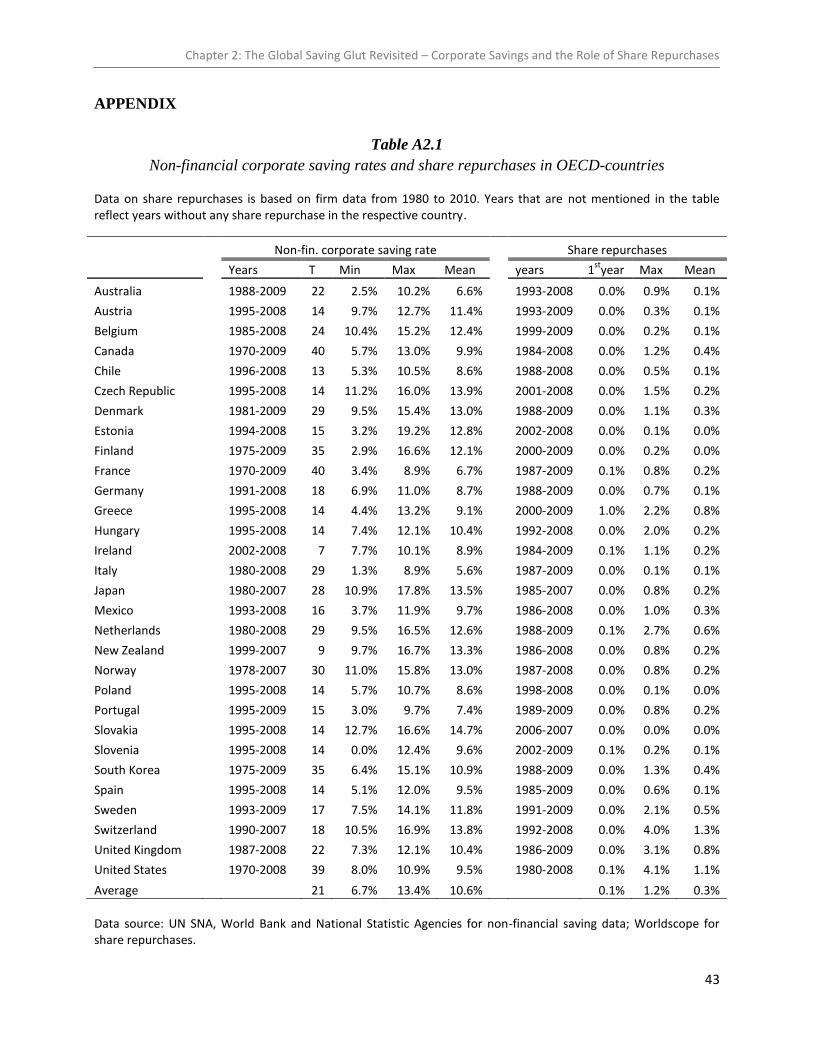
Chapter 2: The Global Saving Glut Revisited – Corporate Savings and the Role of Share Repurchases
43
APPENDIX
Table A2.1
Non-financial corporate saving rates and share repurchases in OECD-countries
Data on share repurchases is based on firm data from 1980 to 2010. Years that are not mentioned in the table reflect years without any share repurchase in the respective country.
Non-fin. corporate saving rate Share repurchases
Years T Min Max Mean
years 1
styear Max Mean
Australia
1988-2009 22 2.5% 10.2% 6.6%
1993-2008 0.0% 0.9% 0.1%
Austria
1995-2008 14 9.7% 12.7% 11.4%
1993-2009 0.0% 0.3% 0.1%
Belgium
1985-2008 24 10.4% 15.2% 12.4%
1999-2009 0.0% 0.2% 0.1%
Canada
1970-2009 40 5.7% 13.0% 9.9%
1984-2008 0.0% 1.2% 0.4%
Chile
1996-2008 13 5.3% 10.5% 8.6%
1988-2008 0.0% 0.5% 0.1%
Czech Republic
1995-2008 14 11.2% 16.0% 13.9%
2001-2008 0.0% 1.5% 0.2%
Denmark
1981-2009 29 9.5% 15.4% 13.0%
1988-2009 0.0% 1.1% 0.3%
Estonia
1994-2008 15 3.2% 19.2% 12.8%
2002-2008 0.0% 0.1% 0.0%
Finland
1975-2009 35 2.9% 16.6% 12.1%
2000-2009 0.0% 0.2% 0.0%
France
1970-2009 40 3.4% 8.9% 6.7%
1987-2009 0.1% 0.8% 0.2%
Germany
1991-2008 18 6.9% 11.0% 8.7%
1988-2009 0.0% 0.7% 0.1%
Greece
1995-2008 14 4.4% 13.2% 9.1%
2000-2009 1.0% 2.2% 0.8%
Hungary
1995-2008 14 7.4% 12.1% 10.4%
1992-2008 0.0% 2.0% 0.2%
Ireland
2002-2008 7 7.7% 10.1% 8.9%
1984-2009 0.1% 1.1% 0.2%
Italy
1980-2008 29 1.3% 8.9% 5.6%
1987-2009 0.0% 0.1% 0.1%
Japan
1980-2007 28 10.9% 17.8% 13.5%
1985-2007 0.0% 0.8% 0.2%
Mexico
1993-2008 16 3.7% 11.9% 9.7%
1986-2008 0.0% 1.0% 0.3%
Netherlands
1980-2008 29 9.5% 16.5% 12.6%
1988-2009 0.1% 2.7% 0.6%
New Zealand
1999-2007 9 9.7% 16.7% 13.3%
1986-2008 0.0% 0.8% 0.2%
Norway
1978-2007 30 11.0% 15.8% 13.0%
1987-2008 0.0% 0.8% 0.2%
Poland
1995-2008 14 5.7% 10.7% 8.6%
1998-2008 0.0% 0.1% 0.0%
Portugal
1995-2009 15 3.0% 9.7% 7.4%
1989-2009 0.0% 0.8% 0.2%
Slovakia
1995-2008 14 12.7% 16.6% 14.7%
2006-2007 0.0% 0.0% 0.0%
Slovenia
1995-2008 14 0.0% 12.4% 9.6%
2002-2009 0.1% 0.2% 0.1%
South Korea
1975-2009 35 6.4% 15.1% 10.9%
1988-2009 0.0% 1.3% 0.4%
Spain
1995-2008 14 5.1% 12.0% 9.5%
1985-2009 0.0% 0.6% 0.1%
Sweden
1993-2009 17 7.5% 14.1% 11.8%
1991-2009 0.0% 2.1% 0.5%
Switzerland
1990-2007 18 10.5% 16.9% 13.8%
1992-2008 0.0% 4.0% 1.3%
United Kingdom
1987-2008 22 7.3% 12.1% 10.4%
1986-2009 0.0% 3.1% 0.8%
United States 1970-2008 39 8.0% 10.9% 9.5% 1980-2008 0.1% 4.1% 1.1%
Average
21 6.7% 13.4% 10.6%
0.1% 1.2% 0.3%
Data source: UN SNA, World Bank and National Statistic Agencies for non-financial saving data; Worldscope for share repurchases.

Chapter 2: The Global Saving Glut Revisited – Corporate Savings and the Role of Share Repurchases
44
Table A2.2
Share repurchases on a firm level
Table A2.2 includes active and inactive companies. Only countries with more than 100 companies in the Worldscope database are included in this table.
# of companies with share repurchases between Share of companies that uses share
repurchases Country # of
companies 1980 and 1999 2000 and 2010 1980 and 2010 Australia 2,072 68 465 484 23%
Austria 106 1 47 47 44%
Belgium 162 1 68 68 42%
Brazil 388 38 123 136 35%
Canada 1,750 219 465 517 30%
Chile 213 4 26 28 13%
China 2,518 5 114 118 5%
Denmark 203 41 107 113 56%
Finland 130 22 60 64 49%
France 895 29 364 370 41%
Germany 1,101 17 250 254 23%
Greece 305 1 78 78 26%
Hong Kong 1,078 161 334 402 37%
India 2,325 43 424 441 19%
Indonesia 418 7 52 57 14%
Israel 248 13 86 90 36%
Italy 301 19 135 138 46%
Japan 3,985 106 1,636 1,652 41%
Kuwait 183 0 116 116 63%
Malaysia 1,049 29 258 271 26%
Mexico 134 50 83 91 68%
Netherlands 205 50 118 126 61%
New Zealand 156 7 28 30 19%
Norway 239 16 87 89 37%
Pakistan 164 2 1 3 2%
Philippines 253 32 73 83 33%
Poland 373 4 72 74 20%
Russia 295 3 89 89 30%
Saudi Arabia 125 0 9 9 7%
Singapore 688 11 154 159 23%
South Africa 393 23 147 154 39%
South Korea 1,266 207 796 816 64%
Spain 163 37 113 119 73%
Sweden 470 11 103 106 23%
Switzerland 289 26 217 217 75%
Taiwan 1,569 24 430 433 28%
Thailand 559 3 64 65 12%
Turkey 243 1 8 9 4%
United Kingd. 2,403 316 1,060 1,117 46%
United States 9,687 3,214 5,094 5,694 59%

Chapter 2: The Global Saving Glut Revisited – Corporate Savings and the Role of Share Repurchases
45
Table A2.3
Overview of variables in dataset
All variables are generally suited for a panel data analysis as there are (1) high variations across the dataset (overall), (2) high variations between the countries (between) and (3) high variations within the countries (within). N gives the overall number of observations for each variable. n gives the number of countries and T-bar gives the average time period covered per country per variable. All variables but cpi, GDPg and d_GDPg are given as ratio over GDP.
Variable Mean Std.Dev. Min Max Observations
Saving overall
0.107 0.032 0.000 0.192
N = 598
between
0.024 0.056 0.147
n = 30
within
0.020 0.011 0.170
T-bar = 19.9
Saving_New overall
0.104 0.031 0.000 0.192
N = 598
between
0.024 0.055 0.147
n = 30
within
0.020 0.008 0.168
T-bar = 19.9
LSaving overall
0.106 0.031 0.000 0.192
N = 578
between
0.024 0.056 0.146
n = 30
within
0.020 0.011 0.170
T-bar = 19.3
LSaving_New overall
0.104 0.031 0.000 0.192
N = 578
between
0.024 0.056 0.146
n = 30
within
0.020 0.008 0.168
T-bar = 19.3
Buybacks overall
0.002 0.005 0.000 0.041
N = 900
between
0.002 0.000 0.010
n = 30
within
0.004 -0.008 0.035
T = 30
Profits overall
0.210 0.058 0.000 0.436
N = 606
between
0.062 0.120 0.407
n = 30
within
0.025 0.078 0.320
T-bar = 20.2
Inv overall
0.125 0.034 0.001 0.252
N = 598
between
0.031 0.074 0.197
n = 30
within
0.017 -0.004 0.191
T-bar = 19.9
GDPg overall
2.841 2.868 -14.570 12.280
N = 854
between
1.052 1.711 6.323
n = 30
within
2.669 -14.520 10.630
T-bar = 28.5
d_GDPg overall
-0.047 2.675 -15.060 16.340
N = 847
between
0.283 -0.353 0.828
n = 30
within
2.665 -14.982 16.526
T-bar = 28.2
cpi overall
8.228 23.803 -13.850 555.380
N = 828
between
9.345 1.332 46.645
n = 30
within
21.831 -37.627 516.963
T-bar = 27.6
finsystem overall
0.803 0.433 0.087 2.107
N = 827
between
0.339 0.176 1.474
n = 30
within 0.277 0.047 2.198 T-bar = 27.6

Chapter 2: The Global Saving Glut Revisited – Corporate Savings and the Role of Share Repurchases
46
Table A2.4
Firm-level correlation matrix of dependent and independent variables
The adjusted saving rate (saving rate less share repurchases) is labeled Saving_New. The prefix L indicates the first lag of a variable. The number of observations is 14,842. Correlation coefficients that are insignificant at the 5% level are written bold in italics.
Variable Saving LSaving Saving _New
LSaving _New
Buybacks/ Assets
Profits/ Assets
Capex/ Assets
Log- assets cpi GDPg d_GDPg
Saving 1.000
LSaving .481 1.000
Saving_New .943 .442 1.000
LSaving_New .435 .924 .422 1.000
Buybacks/ Assets
.101 .085 -.235 .007 1.000
Profits/ Assets
.567 .220 .542 .202 .035 1.000
Capex/ Assets
.198 .219 .199 .215 -.017 0.118 1.000
Logassets -.076 -.122 -.082 -.130 .023 -.002 -.005 1.000
cpi .066 .063 .059 .060 .018 .04 .086 -.058 1.000
GDPg .092 .040 .086 .053 .011 .053 .099 -.02 .252 1.000
d_GDPg .064 .010 .066 .029 -.011 .033 .049 -.012 .114 .780 1.000
Finsystem -.024 .020 -.059 -.027 .106 -.047 -.095 -.074 -.068 -.356 -.382

Chapter 2: The Global Saving Glut Revisited – Corporate Savings and the Role of Share Repurchases
47
Figure A2.1
Piercing the corporate veil? – private and corporate sector saving
Private sector (household and corporate) saving rates on the vertical axis and corporate sector saving rates on the horizontal axes are shown as percentage of GDP and cover the years 1980 to 2008. The dashed line shows the values at which corporate savings would make up 100% of private savings.
Data source: UN SNA, Reserve Bank of India, BIS, National Statistic Agencies.

48
CHAPTER 3
The Effect of Household Debt on Unemployment
– Evidence from Europe and Spanish Provinces
Abstract
Most European countries faced steep and persistent increases in unemployment following the
financial crisis of 2007-08. With this study we seek to investigate whether some part of these
increases can be attributed to indebted households who reduced their consumption in order to
restructure their balance sheets. We establish a link between household debt and aggregate
demand based on a cross-country study of 18 European countries and show how household sector
debt affects unemployment via the aggregate demand channel. We strengthen the results with an
analysis of Spanish provinces. The level of household sector debt in Spanish provinces is highly
significant in determining the increase in provincial unemployment from 2007 to 2010 via the
aggregate demand channel. We find that on aggregate, approximately 1/3 of the increase in
Spanish unemployment can be traced back to high household debt levels.

Chapter 3: The Effect of Household Debt on Unemployment – Evidence from Europe and Spanish Provinces
49
3.1 INTRODUCTION
Many countries in the world are now in their sixth year of economic crisis. The downturn began
in the United States with the subprime crisis. Low interest rates and rising house prices, together
with an unregulated subprime mortgage market, encouraged an increasing number of Americans
to fulfill their lifelong dreams of buying their own apartments or houses or moving into larger
and fancier homes. In 2006-2007, the housing bubble burst, first home owners, then banks and
finally real sector companies came under distress. This subprime crisis led to the global financial
crisis in 2007-2008, which, in most of the economies of the developed world, was followed by a
deep recession beginning in 2008-2009. This recession was accompanied by increasing
unemployment rates and debt-financed government programs intended to support the economy.
Today, in 2012, many economies around the world continue to suffer from high unemployment
rates and debt levels that exceed the pre-crisis levels.
All of the episodes of this long-lasting crisis period are closely linked to debt. First, households
realized their over-indebtedness after the real estate bubble burst. Then, issues with financial
sector debt and leverage led to a systemic financial crisis. Since 2010, it is government debt that
worries rating agencies, investors who have purchased government bonds and the public, who
ultimately guarantees public debt through the tax basis. To non-economists, it appears obvious
that substantial debt loads are a source of worry. A larger nominal amount of debt leads to higher
debt service burdens. The more a household, bank, corporation or state has to pay in interest, the
less money is available for consumption and investment if the household or organization’s
income remains constant. Once the debt service becomes too high, bankruptcy occurs.
This situation may also be viewed differently. The debt of one person, corporation or state is
wealth of another person, corporation or state. If John Doe must service a debt of 10,000 dollars
and pays interest of 10% on that debt, he loses 1,000 dollars that he could otherwise spend.
However, if Jane Doe lent 10,000 dollars to John, she now has an additional 1,000 dollars to
spend. The same is true for a government. When the government must pay more interest on its
debt, the lender receives these higher interest payments and spends the money. Thus, in a closed
economy or more precisely if the net foreign asset position and the resulting net income are
insignificant, the majority of the interest should be paid and received within the country, with the

Chapter 3: The Effect of Household Debt on Unemployment – Evidence from Europe and Spanish Provinces
50
two amounts canceling each other out. Based on this line of argument, do we really need to care
about debt levels or is the public debate falling for a zero-sum game?
This paper contributes to the academic and public debate regarding the relationship between debt
and aggregate demand and its effect on unemployment. Theory might give reasons for believing
that the debt levels itself need not be a source of concern, though even the theoretical evidence is
far from conclusive. Nevertheless, although the research in this area remains controversial, the
amount of empirical work being conducted on this relationship is increasing. Two recent and very
influential analyses that will be discussed in further detail later in this paper are the studies by
Mian and Sufi (2012) and Dynan (2012). However, both of these papers focus on the United
States.
This paper instead looks at Europe and investigates how the level of household debt and the
changes in household debt are linked to aggregate demand in this region which translates into
unemployment. The household sector is the focus of this paper because of the importance of
household consumption expenditure to aggregate demand and because the household debt in
many European countries increased rapidly prior to the crisis, whereas government deficits and
debt levels exhibited rather modest increases or even decreases in many countries. Furthermore,
there is substantial variation in the development of household debt among and within European
countries. A comparison of 18 European countries shows that there is a high and significant
correlation between the debt build-up prior to 2007 and the changes in employment that occurred
from 2008 to 2010. The economic performance of these countries has suffered because of the end
of the debt-fueled growth there and in some cases because of a decline in outstanding debt. Thus,
there appears to be a link between changes in debt and aggregate demand.
The underlying transmission mechanism that is investigated in this study begins with a shock to
the balance sheets of individual households. The shock for households is greater if they must
expend more effort to restructure their balance sheets. The more debt a household has
accumulated relative to its income before the shock occurred, the more deleveraging the
household must arrange by increasing savings and reducing spending after the shock to
restructure its balance sheet. Given the elasticity of employment with respect to demand, these
changes generate increased unemployment.

Chapter 3: The Effect of Household Debt on Unemployment – Evidence from Europe and Spanish Provinces
51
There are at least two different theoretical mechanisms that could explain the deleveraging needs
of households. First, these deleveraging needs may be a function of increased credit constraints
or, to put it differently, of falling debt limits due to lower collateral values. Eggertsson and
Krugman (2012) model the deleveraging needs of borrowing households using an exogenous
decrease in the debt limit. If the real interest rate cannot adjust to its natural or full employment
level, aggregate demand will fall. Second, the deleveraging needs of households may also be a
function of changing perceptions of lifetime income or wealth. For instance, housing prices,
which determine the value of one of the most important assets for most households, almost
certainly affect household wealth (or indebtedness). It is now generally understood that the
Spanish housing market experienced a significant boom in the early 2000s and that this boom
ended rather abruptly in 2007. Thus, it appears very likely that Spanish households not only were
forced to deleverage due to more tightly binding credit constraints as their collateral lost value
but also suffered large decreases in their net wealth. In addition to the disruptions at the real
estate market, the crisis made clear to many Spaniards that future income levels would be smaller
than expected. All three, the credit constraints, the wealth effects and the adjusted expectations
about life time income may explain the increased deleveraging needs of the indebted Spanish
household sector. We will try to disentangle these effects in our empirical analysis by controlling
for housing prices.
Importantly, because aggregate demand will decline more in regions with higher deleveraging
needs than in those with lower deleveraging needs, we should see different responses in regional
sectoral unemployment rates depending on whether we analyze the tradable or non-tradable
sectors (cf. Mian and Sufi (2012)). More precisely, tradable sector employment (unemployment)
in each region, which depends on the aggregate demand from all regions, should fall (rise)
irrespective of the particular deleveraging needs of that specific region. However, the opposite
should be true for the non-tradable sector. In the non-tradable sector, employment
(unemployment) should fall more (rise more) in those regions that have high deleveraging needs.
In a sense, by selling tradable goods, the tradable sector employment insures itself against
idiosyncratic regional demand shocks. Non-tradable sector employment, however, is vulnerable
to regional demand shocks. Thus, if the Spanish provinces’ debt-to-GDP levels are good
indicators of the deleveraging needs that followed the shock to those provinces, the demand
channel predicts higher increases in unemployment in the non-tradable sector in those provinces

Chapter 3: The Effect of Household Debt on Unemployment – Evidence from Europe and Spanish Provinces
52
that had high debt-to-GDP ratios, whereas the increases in tradable-sector unemployment should
be independent of those debt-to-GDP ratios.
We find that these theoretical mechanisms hold for the European country data, which we use in
section 3.3. Section 3.4 presents a more granular analysis based on the regional data for Spain.
This analysis supports the finding that high household debt levels decrease consumption and
aggregate demand and lead to increasing unemployment. Based on this evidence of the role of
debt in aggregate demand and unemployment in Spain, we calculate the magnitude of this effect
using our findings for unemployment in the non-tradable sector. We find that approximately 1/3
of the increase in the aggregate Spanish unemployment between November 2007 and November
2010 is due to debt-related decreases in household spending.
The remainder of the chapter is structured as follows. Section 3.2 provides an overview of the
related literature. Section 3.3 describes a cross-country study of 18 European countries. Section
3.4 presents the within-country study of Spain, including the calculation of the aggregate effect of
debt on unemployment. Section 3.5 concludes the chapter.
3.2 OVERVIEW OF RELATED LITERATURE
The effect of household debt on the economy has been repeatedly examined in combination with
recessions. Fisher (1933) postulated the debt deflation theory for great depressions. Mishkin
(1978) empirically examined the Great Depression and considered how household balance sheets
served as a transmission mechanism for changes in aggregate demand. The American recession
of 1973-75 is empirically investigated by Mishkin, Gordon and Hymans (1977), who focus on the
role of household debt and stock market developments. All of these papers find an important
negative effect of debt on economic activity. However, whereas Fisher (1933) examines the
effect on asset prices, Mishkin (1978) and Mishkin et al. (1977) focus on consumption and
aggregate demand. Palley (1994) builds a model of the effects of household debt on aggregate
demand based on the different propensities to consume among creditor and debtor households
and applies the model to the recession of the early nineties. Palley (1994) concludes that
increases in household debt fuel aggregate demand but that the servicing of this debt
subsequently lowers aggregate demand. The financial crisis and economic downturn of 2007-09

Chapter 3: The Effect of Household Debt on Unemployment – Evidence from Europe and Spanish Provinces
53
have again drawn attention to the role of household sector debt. Keen (2009) emphasizes the role
of debt in aggregate demand. Changes in the volume of debt as a percentage of GDP explain how
much of the aggregate demand is debt financed. Keen (2009) validates the link between the
household debt and aggregate demand for Australia by showing how both increasing debt and
declining unemployment and decreasing debt and rising unemployment move together. The link
between household debt and aggregate demand in the recent recession is evident for the United
States in Mian and Sufi (2012) and Dynan (2012). Dynan (2012) uses the Panel Study of Income
Dynamics (PSID) to examine the effect of household debt on consumption. She estimates the
effect of leverage and that of debt service burdens on the changes in consumption that occurred
from 2007 to 2009 and confirms that a significant negative impact exists even after income and
wealth effects are controlled for. This approach provides a microfoundation for the deleveraging
shock that depresses consumption in addition to wealth and income effects.
Overall, this chapter is most closely related to the work by Mian and Sufi (2012), which
investigates the link between household sector debt levels and aggregate demand with a regional
analysis. These authors use county-level data from the United States and estimate how household
debt levels, measured as debt over income, influence consumption, which fuels aggregate
demand. The size of the debt level is interpreted as the magnitude of the household balance sheet
shock and of the need for adjustment to household-level finances. Mian, Rao and Sufi (2012) use
local retail sales data to show that household debt levels affect consumption. Having illustrated
the link between household debt and consumption, Mian and Sufi (2012) use the elasticity of
employment to aggregate demand to measure the transmission of household debt via
consumption and aggregate demand on employment and thus, to the severity of the crisis in the
United States. The distinction between employment in the tradable and non-tradable sectors is
important to the analysis. The demand for tradable goods is determined on a national level, which
renders the shocks to the household balance sheet in one county unimportant. The demand for
non-tradable goods, in contrast, is only dependent on local consumption. Thus, regional
employment in tradable industries is independent of local debt levels, and employment in non-
tradable industries should be highly dependent on local debt levels. Mian and Sufi (2012) confirm
the validity of their model by regressing the changes in total employment, tradable employment
and non-tradable employment from 2007 to 2009 on the 2006 debt to income ratio. Controlling

Chapter 3: The Effect of Household Debt on Unemployment – Evidence from Europe and Spanish Provinces
54
for structural shocks by including the shares of the construction, tradable and non-tradable
industries does not change the outcome.
The International Monetary Fund (2012) and the McKinsey Global Institute (2010, 2012) reports
cover more than one country. The IMF finds that larger increases in household debt lead to more
severe recessions and examines country-level case studies in seeking to determine how to address
large household debts and house price decreases. The McKinsey Global Institute examines
deleveraging across all economic sectors and describes how historic deleveraging processes have
taken place (cf. McKinsey Global Institute (2010)) and how the major economies have
meanwhile progressed in their deleveraging process (cf. McKinsey Global Institute (2012)). The
case studies presented in that report suggest that during an economy-wide deleveraging, a country
should begin with deleveraging in the private sector while the public sector compensates for the
loss in aggregate demand; then, the latter should begin deleveraging once the nation’s economic
growth regains its momentum.
This study contributes to the literature by using existing approaches to investigate household debt
and aggregate demand in Europe and particularly in Spain and its provinces. This research can
thus confirm that the previous results for the United States and Australia are also valid for a
legally and culturally quite different region. Furthermore, this research indicates which portion of
the increase in Spanish unemployment is traceable to the high household sector debt. Thus, this
chapter provides a fact base for Spanish policy makers as well as for macro-prudential regulators
who are concerned with the effects of household sector debt on the economy.
3.3 HOUSEHOLD DEBT AND UNEMPLOYMENT – A EUROPEAN PERSPECTIVE
To investigate whether there is a link between household debt and aggregate demand in Europe,
one can compare the debt data for European countries to two indicators for aggregate demand.
One possible measure of the effect of debt on aggregate demand is the contribution of household
consumption expenditure to GDP growth. The other (more indirect) measure of aggregate
demand is employment, which is suitable because of the high elasticity of employment to
aggregate demand, albeit with some time delay. The hypotheses tested in this research are as
follows:

Chapter 3: The Effect of Household Debt on Unemployment – Evidence from Europe and Spanish Provinces
55
Regions with (1) larger increases in debt or (2) higher debt levels prior to an economic
downturn will experience a lower growth of aggregate demand during an economic
downturn than regions with (1) smaller increases in debt or (2) lower debt levels because
of household balance sheet restructuring.
Lower growth of aggregate demand means thereby that it can also turn negative. The
transmission mechanism of household debt to aggregate demand is as described by Keen (2009),
Mian and Sufi (2012) or Dynan (2012). Using the permanent income hypothesis (PIH) or life
cycle hypothesis (LCH), the households that expect higher future income (PIH) or that benefit
from increased housing wealth (LCH) should adapt their consumption behavior and consume
more. If the household’s expectations regarding future income are sufficiently high, the
household can rationally take on debt today to smooth consumption. When a negative exogenous
shock lowers the expectations of the household, the individuals in the household will need to
change their consumption and investment behavior accordingly. Households that have increased
their debt more than others or that hold higher debt levels must reduce their debt by a larger
amount. The household balance sheet is restructured through reductions in consumption
spending. Still, it is not unquestionable that the aggregate demand is affected by the households
that restructure their balance sheets. Households that have acted as lenders in the first place will
have the option to consume more when the debt is repaid. Thus, in aggregate, there should be no
effect on aggregate demand if the propensity to consume out of income is the same across
households. Nevertheless, the aggregate demand might indeed be reduced if the debt overhang is
sufficiently large and if the economy is stuck at the zero lower bound (cf. Eggertsson and
Krugman (2012)).
To test our hypothesis, we compare changes in household debt as well as levels of household debt
using our two measures of aggregate demand. If we find no effect on spending, the contribution
of household consumption expenditure to GDP growth should be independent of debt. If debt has
no influence on aggregate demand, neither changes in household debt nor the level of household
debt will be linked to the changes in employment that follow aggregate demand. Both hypotheses
are tested using aggregated country-level data for European economies.

Chapter 3: The Effect of Household Debt on Unemployment – Evidence from Europe and Spanish Provinces
56
3.3.1 Data sources
The cross-country study builds on 18 European countries regarding the measure of employment
and 9 euro-area countries regarding the measure of household consumption expenditure’s
contribution to GDP growth. All of the debt data are obtained from Eurostat’s annual sector
accounts and are amended using data from the national statistical agencies and central banks
when the Eurostat data coverage is insufficient. Household debt is used as provided by Eurostat
(total financial liabilities of the household sector including non-profit institutions serving
households). The GDP and disposable income data are also based on Eurostat’s annual sector
accounts. To establish the link between household sector consumption expenditure and its
contribution to GDP growth, data from the European Central Bank are used. These data are
captured on a quarterly basis but are not provided for all euro-area countries, which limits the
number of observations to 9 countries. The second test of the hypotheses uses employment data
from the EU’s Labor Force Survey, which are sourced from Eurostat.
3.3.2 Empirical analysis
The American subprime crisis in 2007 only spread to the European real economy in 2008. There
was a peak in debt issuance in 2007 and a peak in employment in 2008. Thus, 2007 serves as a
starting point for our analysis of the effects of household debt on aggregate demand. We argue
that debt levels and changes in debt have an effect on consumption and, consequently, on
aggregate demand. The transmission channel is the necessary restructuring of the household
balance sheet. In a boom period, a household takes on debt, anticipating increases in future
income and asset prices. The household spends this debt on the purchase of assets, the most
important of which is housing, and on consumption expenditure. When the boom period ends,
asset prices stagnate or shrink, and future income streams become more uncertain. Households
consequently restructure their balance sheets in accordance with their updated expectations. The
restructuring of balance sheets comes along with increasing saving and decreasing consumption
expenditure. The higher the debt level of the household sector, the larger the amount of debt that
the sector must repay and the greater the reduction in consumption and, thus, aggregate demand.
The same rule holds for changes in debt. The higher the increase in debt prior to the shock, the
greater is the need to pay back debt and save after the peak of the boom. Both measures, changes
in debt and the level of debt, are important. The level of debt is a good indicator because there is

Chapter 3: The Effect of Household Debt on Unemployment – Evidence from Europe and Spanish Provinces
57
a natural limit to household debt in terms of debt service. The more debt a household sector
holds, the larger the debt service burden, and this burden cannot exceed disposable income if one
rules out Ponzi games. The increase in debt serves as a good indicator for the magnitude of the
shock because it shows how far households have deviated from their usual level of debt. If
interest rates do not change, an increase in the debt-to-income ratio will alter the debt service
burden proportionally. If the aggregated household sector long-term consumption behavior does
not change accordingly, a short-term drop in consumption must occur to soften the process of
adjustment to the previous debt-to-income ratios. This drop in consumption will dampen the
aggregate demand and, consequently, will decrease employment. For there to be an effect on
aggregate demand, it is not even necessary for there to be a nominal decrease in debt volume. A
reduction in the debt growth rate is sufficient to reduce the aggregate demand relative to previous
periods when the income levels do not change because the total amount that is available for
consumption is reduced. The first method of validating this line of argument involves
demonstrating the high correlation between changes in debt and the contribution of household
consumption expenditure to GDP growth, as shown in figure 3.1.
Figure 3.1
Changes in household sector debt and contribution of consumption expenditure to GDP growth
Household sector debt is measured in euro. Changes in debt and the contribution of household consumption expenditure to GDP growth are measured quarterly as a moving average over four quarters. The countries included (time span covered) are Austria (2003-2011), Belgium (1997-2011), France (1996-2011), Germany (1992-2011), Ireland (2002-2011), Italy (1998-2011), the Netherlands (2000-2011), Portugal (1998-2011) and Spain (2001-2011).
Data source: National Central Banks, European Central Bank.
Contr. of cons. = 11.061 ∆debt - 0.0221 R² = 0.356; p-value of ∆debt: 0.000
-150%
-100%
-50%
0%
50%
100%
150%
-3% -1% 1% 3% 5% 7% 9%
Co
ntr
ibu
tio
n o
f co
nsu
mp
tio
n
exp
en
dit
ure
to
GD
P g
row
th
qu
arte
rly,
in p
erce
nt
Change in nominal household sector debt quarterly, in percent

Chapter 3: The Effect of Household Debt on Unemployment – Evidence from Europe and Spanish Provinces
58
Most of the data points in figure 3.1 show that nominal debt is, in fact, increasing; the nominal
deleveraging in countries such as Spain only began in 2010. A nominal quarterly increase below
0.5% may still be considered to indicate real deleveraging if the inflation rate is close to 2%.
When we compare the extremes in this figure – e.g., increases below 0.5% and above 3.0% – it is
clear that high debt growth is associated with a high share of consumption contribution to GDP
growth, whereas when debt grows slowly or declines, the contribution of consumption to GDP
growth is low or negative. Thus, figure 3.1 has two implications. First, mortgages, which
represent the largest fraction of household sector debt, are not exclusively linked to housing
expenditures. Second, an increase in household debt will be accompanied by an increasing
positive impact of household consumption expenditure on GDP growth. One might expect
changes in European household debt not to be closely linked to consumption because most debt is
used to purchase housing assets. However, due to the positive correlation between increases in
household debt and the contribution of consumption to GDP growth, even though direct
mortgage equity withdrawals are of minor importance in Europe, a higher volume of real estate
mortgages is still associated with a higher contribution of consumption to GDP growth. This
connection may be a function of indirect effects such as wealth effects. The connection may also
be explained by the PIH. The data that show increasing nominal debt stem from the years after
the introduction of the common currency in Europe. The introduction of the euro, especially in
the Mediterranean, led to a reduction in credit constraints. This development, together with the
capital inflows from Northern Europe, fed people’s expectations regarding their future incomes,
which they expected to be permanently higher. These expectations, together with low interest
rates, encouraged housing investments (which appeared to be more affordable) and higher
consumption based on the positive economic outlook. The PIH not only holds in upward markets
but is valid for downturns as well. The shock of the financial crisis, whose size varied from
country to country depending on the debt-to-income ratios of the various nations as stated in our
hypothesis, generated lower expectations regarding income. In turn, lower lifetime incomes
required the restructuring of household balance sheets, i.e., reductions in debt through increased
saving and reduced consumption.
This relationship also exists beyond the pooled euro area. A closer look at the single countries in
the currency union confirms the results (cf. table A3.1). Eight of the nine euro-area countries
under consideration show a high correlation between changes in household sector debt and the

Chapter 3: The Effect of Household Debt on Unemployment – Evidence from Europe and Spanish Provinces
59
contribution of household consumption expenditure to GDP growth; Belgium is the only country
without this link. Furthermore, in the countries for which we have data for longer time periods,
the correlation was especially strong during the last decade – in the years preceding the crisis and
during the crisis itself. The next interesting result is that the countries that face the most severe
problems in the euro crisis are those with the highest correlation between changes in debt and the
contribution of consumption expenditure to GDP growth. Ireland, Portugal and Spain have
correlation coefficients of approximately 80%, and Italy’s coefficient for the period from 2000 to
2011 is 65.6%.21
These data may suggest that debt-financed, consumption-driven GDP growth is
vulnerable to shocks. The high correlation coefficients for the Mediterranean countries relative to
Austria, Germany or the Netherlands may result from the debt boom after the introduction of the
euro. Whereas the latter countries were used to low inflation rates and rather low interest rates,
the former benefitted more from the introduction of the euro in this regard. The decreasing
interest rates stimulated demand for credit that was partially provided by the northern euro
countries. The increasing provision of credit and capital inflows stimulated these economies and
encouraged consumption spending. This trend partially explains why the country-level
correlation between the changes in credit and the contribution of consumption to GDP growth is
higher for the years preceding the crisis, i.e., the years following the introduction of the euro.
Explicitly grouping the observations into those from the period prior to the crisis and those from
during the crisis (cf. figure A3.1(a)) reveals that the slope of the relation between the changes in
debt and the contribution of consumption expenditure to GDP growth is 1.5 times steeper during
the crisis, though the explanatory power of these findings is smaller. In addition, analyzing the
data from the worst-affected countries and the more stable countries (cf. figure A3.1(b)) shows
that the contribution of consumption expenditure to GDP growth in the pooled, stable countries is
marginal, whereas we observe a steep slope and high explanatory power of debt for the other
group. Our first measure of aggregate demand thus works for these subsamples and for the euro
area more generally, but its quality depends on the precise sample composition.
The second and more indirect measure of aggregate demand is illustrated in figure 3.2, which
shows the high correlation between the changes in debt prior to the crisis and the subsequent
magnitude of the changes in employment.
21
Using quarterly data instead of smoothed moving average data also yields high and significant coefficients.

Chapter 3: The Effect of Household Debt on Unemployment – Evidence from Europe and Spanish Provinces
60
Figure 3.2
Changes in household sector debt and employment
Household sector debt is measured as the ratio of financial liabilities to disposable income. Employment is measured as the ratio of the employed population aged 15 to 64 to the total population aged 15 to 64. The number of European countries included is 18.
Data source: Eurostat.
The hypothesis that a larger increase in the debt ratio leads to a stronger decline in employment is
confirmed for the 18 European countries for which data for both debt and employment are
available for the relevant time span. The correlation coefficient of -69.2% demonstrates the
substantial negative relationship between increases in household debt and the subsequent
adjustments in aggregate demand. A regression without further control variables indicates that for
every increase in debt of 10 percentage points from 2000 to 2007, the employment ratio
decreased by 0.6 percentage points from 2008 to 2010.
The level of household sector debt can be used in lieu of the increase in household sector debt.
Household sector debt relative to disposable income prior to the crisis is depicted in figure 3.3.
∆employment = -0.0645 ∆debt + 0.255 R² = 0.4795; p-value of ∆debt: 0.002
-10
-08
-06
-04
-02
00
02
04
-20 0 20 40 60 80 100
Ch
ange
in e
mp
loym
en
t ra
tio
fro
m 2
00
8-1
0
in p
erce
nta
ge p
oin
ts
Change in household sector debt from 2000-07 in percentage points

Chapter 3: The Effect of Household Debt on Unemployment – Evidence from Europe and Spanish Provinces
61
Figure 3.3
Levels of household sector debt and changes in employment
Figure 3.3(a) includes the same 18 countries as figure 3.2. Figure 3.3(b) presents a country sample that excludes the outliers Lithuania and Latvia.
Data source: Eurostat.
Using the same country sample to test this paper’s underlying hypothesis fails to prove the
hypothesis, and it appears as though the level of household sector debt is irrelevant. However,
there are two outliers in the country sample: Latvia and Lithuania. Both countries had very low
levels of household debt in the 1990s and experienced a substantial increase in household debt
prior to the crisis. Given the small size of our sample the outliers can have a significant effect on
the outcome of the analysis, we therefore exclude Latvia and Lithuania due to their structural
differences from other European countries. This step further backs the hypothesis regarding the
effect of debt on aggregate demand (cf. figure 3.3(b)). Increases in debt and levels of debt during
a boom are good indicators of the magnitude of the changes in aggregate demand that will occur
Latvia
Lithuania
∆empl. = -0.4589debt - 1.9665 R² = 0.0175; p-value of debt: 0.600
-10
-08
-06
-04
-02
00
02
04
06
0 1 2 3
Ch
ange
in t
he
em
plo
yme
nt
rate
fro
m 2
00
8-1
0,
in p
erce
nta
ge p
oin
ts
Household sector debt in 2007 ratio over disposable income
Figure 3.3(a) (Correlation: -13.2%)
∆empl. = -1.2774debt - 0.1826 R² = 0.3238; p-value of debt: 0.021
-10
-08
-06
-04
-02
00
02
04
06
0 1 2 3
Household sector debt in 2007 ratio over disposable income
Figure 3.3(b) (Correlation: -56.9%)

Chapter 3: The Effect of Household Debt on Unemployment – Evidence from Europe and Spanish Provinces
62
in the downturn.22
The current Eurostat data do not yet include the years 2011 and 2012;
otherwise, it would have been possible to precisely measure the degree of adjustment in
household sector debt: whether the debt growth decreased, whether there was no debt growth at
all or whether there was a nominal reduction in the debt-to-income ratio. The conclusion to be
drawn from the data presented in this section is nevertheless clear. Household sector debt fuels
aggregate demand in an upswing, but during a time of debt moderation, when debt growth
decelerates or becomes negative, the impact on aggregate demand is severe.
This cross-country study therefore provides results that support our hypotheses. We hence
confirm the results of the analyses of American household sector debt deleveraging conducted by
Mian and Sufi (2012) and Dynan (2012) and by Keen (2009) for Australian household sector debt
and aggregate demand. A sharp reduction in debt growth and deleveraging by European
household sectors severely reduced aggregate demand.
3.4 HOUSEHOLD DEBT AND UNEMPLOYMENT – THE CASE OF SPAIN
These 18 European economies are significantly more diverse than Australia or the United States,
so that these results are more likely to be affected by unobserved country characteristics. The low
number of observations also hampers the use of econometric regressions. To address both issues,
this section presents a regional analysis of a single country. Criticism against results from
aggregation on a national level and comparison of European countries is less problematic for a
comparison of more granular regional data. The case of Spain is also used in order to address one
of the countries that is currently most heavily hit by the euro crisis, that experienced particularly
high increases in debt and high levels of debt and that currently suffers from exceptionally high
unemployment rates. Spanish households decreased their nominal debt outstanding in the 1st
quarter of 2009 for the first time in over 20 years. On a yearly basis, modest deleveraging started
in 2009 and paused in 2010; deleveraging accelerated in 2011 (cf. figure 3.4).
When we focus on the Spanish provinces, the number of observations increases to 50,23
which is
a more suitable number for econometric regressions. In addition, the shocks that apply to all
22
The correlation coefficient for these two measures, the level of debt and the increase in debt, is 69% in the sample with 18 countries. Excluding the outliers Latvia and Lithuania increases the correlation coefficient to 81%. 23
Spain has 52 provinces, but the relevant data are only available for 50 provinces.

Chapter 3: The Effect of Household Debt on Unemployment – Evidence from Europe and Spanish Provinces
63
Spanish provinces are more homogenous in nature than the shocks that apply to the 18 European
countries. However, the size of the shocks among provinces in Spain does still vary. By using the
provinces’ debt-to-GDP ratios, we ensure that the shock is heterogeneous in size and is thus
suited to our analysis. Compared to a European analysis, the Spanish economy is more
homogenous in terms of institutions such as the labor market, the educational system, and credit
provisioning. Because we focus on the non-tradable sector, we also benefit from the fact that
structural differences across provinces are larger for industrial production and tradable goods
than for consumption behavior for non-tradable goods. This difference gives further support to
using provincial data from a single country. Therefore, this section focuses on regional analyses
of Spain.
We will first introduce the theoretical foundation of the empirical analysis in section 3.4.2 and
then describe the data, which we use in the empirical analyses (section 3.4.4), for robustness
checks (section 3.4.5) and for the calculation of the share of the increase in Spanish
unemployment that can be traced back to household sector debt (section 3.4.6).
3.4.1 Theoretical framework
The theoretical foundation for the investigation of the effect of household debt via the aggregate
demand channel on unemployment is provided in Mian and Sufi (2012, p. 10 ff. and 29, 30). The
model described here in a short version mirrors the model of Mian and Sufi (2012). Differences
arise because we look at increases in unemployment at a provincial level and the elasticity of
unemployment to a reduction in consumption and aggregate demand instead of employment
losses at a county level and the elasticity of employment with respect to output demand .
The model setup is as follows: households spend a fraction of their income on non-tradable
goods NT and the rest of their income on tradable goods T. When households reduce their
consumption, both, tradable and non-tradable goods are affected. Unemployment reacts to this
reduction in demand and increases according to the elasticity of unemployment to a reduction in
aggregate demand .
In this model, province is hit by the demand shock . However, the total shock to a province
consists of a reduction in demand for non-tradable goods in the respective province and a
reduction in demand for tradable goods from the whole country that hits this province:

Chapter 3: The Effect of Household Debt on Unemployment – Evidence from Europe and Spanish Provinces
64
(3.1)
where is the average shock for tradable goods for each province:
(3.2)
The total demand-driven increase in unemployment in province depends on the elasticity of
unemployment with respect to output, i.e. . Each province is furthermore exposed to a country
wide shock that is equal to all provinces and a structural shock that just affects province .
The total increase in unemployment in a province can thus be written as:
(3.3)
The aggregate increase in unemployment that results from the debt-driven demand shock only
(3.6) can then be calculated as the sum of the increases in unemployment in non-tradable sectors
(3.4) and the sum of the increases in unemployment in tradable sectors (3.5).
(3.4)
(3.5)
(3.6)
To derive econometrically the effect of this demand shock, the structural shock in province and
the country wide shock that affects all provinces equally need to be excluded. By using a narrow
definition for the non-tradable sector that focuses on regional consumption that is not likely to be
prone to a regional structural shock, we aim to exclude from our calculation. The change in
non-tradable sector unemployment for a province that is not exposed to a regional structural
unemployment shock is given by equation (3.7):
(3.7)

Chapter 3: The Effect of Household Debt on Unemployment – Evidence from Europe and Spanish Provinces
65
As a next step, country-wide shocks are excluded by taking the differences between the
provinces. We thereby assume that the decile of provinces with the lowest debt level ( )
does not suffer from a deleveraging shock, but that these provinces are a benchmark for
developments that affect all provinces. We consequently compare all provinces to the province
with the fifth-lowest debt level ( ):
(3.8)
is set to zero for the five provinces with the lowest debt levels.
If we could directly observe the demand shock , the aggregated increase in unemployment in
the non-tradable sector due to a debt-driven reduction in demand could be estimated as
(3.9)
However, we cannot directly measure the demand shock . Therefore we proxy the size of this
demand shock for each province by the level of household debt relative to GDP. Households with
more debt need to reduce their spending by a larger amount. Thus, provinces with higher debt-to-
GDP ratios experience larger drops in aggregate demand and larger increases in unemployment.
We use our indicator of household sector debt in province for the calculation of the increase in
unemployment:
(3.10)
This approach is suitable because we have a linear relationship between household sector debt
levels and changes in non-tradable sector unemployment, which is shown in the empirical
analysis and figure 3.5. The increase in total unemployment that is related to the debt-related
reduction in consumption can then be calculated by solving (3.9) for ; i.e., multiplying the
increase in non-tradable unemployment with the inverse of the share of non-tradable
unemployment in total unemployment:
(3.11)

Chapter 3: The Effect of Household Debt on Unemployment – Evidence from Europe and Spanish Provinces
66
The term is thereby neglected in (3.11) because we make the conservative assumption that
the decile of provinces with the lowest debt levels did not face a demand shock from too high
debt burdens. This approach is taken to the Spanish data in section 3.4.6.
3.4.2 Description of the data
The Spanish regional data are taken from the Instituto Nacional de Éstadística (INE), the Spanish
Ministry of Employment and Social Security (Ministerio de Empleo y Seguridad Social), the
Spanish Ministry of Public Works and Transport (Ministerio de Fomento) and Eurostat. The
regional level used in the analyses is NUTS-3,24
i.e., the Spanish provincias are analyzed.
Because there is no information on the overall household debt levels or the changes in household
debt for the Spanish provinces, we require an alternative measure. This is found in the mortgage
data for the Spanish provinces, which are provided by the INE. Mortgages account for 84% of
total household debt, and this share is almost independent of the income percentiles according to
the survey of household finances.25
Thus, in this research, the volume of mortgages is a good
alternative measure to total household debt. All of the mortgage data are monthly data that is
available from January 2003 onwards. However, there is no information on the total level of
mortgages outstanding but the monthly information indicates the number and volumes of newly
issued mortgages, which we use to proxy the total level of mortgages outstanding. The mortgage
data from the INE are split into different categories. This allows us to focus on housing
mortgages.26
24
NUTS levels (fr. Nomenclature des unités territoriales statistiques – Nomenclature of territorial units for statistics) are used for regional statistics in Europe. NUTS-3 is used to distribute the regional funds of the European Union. 25
The ratio of 2008 mortgage debt to total debt ranges from a maximum of 85.3% for the top income percentile to a minimum of 82.3% for the second highest income percentile. The overall average is 84%. The differences in the income percentiles can be traced to the fact that the highest income percentile uses less than half of its mortgages for main residences, whereas the poorest 40% of households use 87% of their mortgages for main residences (cf. Bank of Spain (2011), p. 111 table 6). 26
The two major categories are agricultural land (which had a share of 6% from January 2003 to April 2011) and urban land (which had a share of 94%). Within urban land, there are multiple categories: housing (61%), lots (11%), and other urban land (22%). “Other urban land” includes commercial properties, garages, offices, and industrial buildings, but also buildings that include dwellings. Using total mortgages instead of housing mortgages generates results that are similar to the ones presented in this section; the significance levels remain the same, although the coefficients are smaller. These results are as expected because the effect of debt taken on for agricultural or business purposes should have less of an effect on household consumption (and, thus, employment in the non-tradable sector) than debt taken on for the purpose of housing.

Chapter 3: The Effect of Household Debt on Unemployment – Evidence from Europe and Spanish Provinces
67
The mortgage data are used in the analyses in two different ways. First, because we do not have
data on the level of household debt, which would allow for a straightforward calculation of the
growth rate as in section 3.3, we compare the aggregated mortgage issuances from 2003 and 2004
over the 2004 GDP with the aggregated mortgage issuances from 2005 to 2007 over the 2007
GDP. This comparison leads us to approximate the growth rate from the three years preceding the
crisis compared to that of the two prior years. It also enables us to investigate the effects of an
increase in mortgage issuances on the subsequent changes in aggregate demand. Second, the
volume of mortgages at a certain point in time can be approximated by the aggregated volume of
newly issued housing mortgages in the five years preceding the crisis, i.e., from January 2003
until December 2007.27
The household mortgage debt calculated in this indirect way is 85.3% of
the total household liabilities in Spain at the end of 2007 (as documented by the Bank of Spain).
This calculated debt level is a really good approximation of the actual debt level because it
almost equals the total mortgage debt of households, which is at 84.1% of total household debt
according to the survey of household finances (cf. Bank of Spain (2011), p. 111). The main
reason why we underestimate the total household debt level is that our measure does not include
credit card debt or personal loans. Our measure can be used if we assume that there is no
systematic difference in the structure of household debt across regions.
For the analysis related to the debt level, we construct a ratio of debt to provincial GDP. The
provincial GDP data that are used to calculate the debt-to-GDP ratios are based on Eurostat
figures. The unweighted mean household sector debt-to-GDP ratio across all provinces was 63%
with a standard deviation of 27%. The average GDP per province in 2007 was 20.2 billion EUR.
Excluding the two most important provinces (Barcelona and Madrid) yields an average GDP of
14.2 billion EUR. Eurostat also serves as the source of the population data used in this study, i.e.,
the data regarding changes in the size of the workforce, which are measured as the percentage
change in the population of individuals between the ages of 15 and 64.
Real estate prices are included in the analysis to determine how the effects of household debt
differ across the provinces that did or did not experience booms in the real estate sector. If the
increase in debt was associated with a parallel increase in real estate prices, then the adjustments
27
Mian and Sufi (2012, p. 12 and 13) use the debt-to-income ratio in their analysis but state that using the accumulation of household debt in the five years preceding the crisis as an alternative measure would not change the results of their analysis.

Chapter 3: The Effect of Household Debt on Unemployment – Evidence from Europe and Spanish Provinces
68
in aggregate demand might result from either real estate price developments or excessive debt
levels. Controlling for real estate prices thus helps us to identify the purely debt-driven aggregate
demand channel. The relevant data are provided by the Spanish Ministry of Public Works and
Transport. All of the prices are mean prices of residential real estate transactions by province and
quarter from 2004 to 2012. The average Spanish residential real estate price in the first quarter of
2004 was approximately 124,000 EUR. The price increased to approximately 190,000 EUR in
the fourth quarter of 2007 (+ 53%) and reached approximately 148,000 EUR in the first quarter
of 2012 (-22% vs. peak, +19% vs. Q1/2004). The unweighted mean increase in the prices across
all provinces from the first quarter of 2004 to the maximum in each province was 89% with a
standard deviation of 44%.
Aggregate demand is measured using the employment and unemployment channel. Employment
rates and total nominal employment figures for the provinces are obtained from the INE. The
Spanish employment rate was 51.1% in the first quarter of 2005. That rate increased to 54.4% in
the third quarter of 2007 and decreased to 45.3% in the first quarter of 2012. The employment
and unemployment rates28
already show a high and significant correlation with the provinces’
household debt figures. To determine the effect of debt on aggregate demand, it is necessary to
identify the portion of unemployment that results from consumption in the individual provinces.
To identify this effect, the unemployment data29
by economic activity on a provincial level are
obtained from the Spanish Ministry of Employment and Social Security. The economic activities
are split into 22 different groups. These groups are then clustered by the type of economic
activity into the tradable sector, the non-tradable sector, construction or other sectors. Due to a
change in the classification system for economic activities that occurred in 2009, we need to
match the earlier classification system with the recoded one (cf. table A3.2). Consequently, not
all of the groups are exactly matched, but the tradable and non-tradable sectors can be identified.
28
We use the term “unemployment” for the sake of simplicity throughout this section, but the data from the Ministry of Employment and Social Security are somewhat broader and also include individuals such as seasonal workers and job seekers who are employed part time but are looking for full time jobs. In November 2007, the ratio of job seekers to total unemployed persons was 147%, indicating a future increase in unemployment. The ratio decreased to 136% in November 2010 and to 133% in September 2012. In 2007 and 2010, the majority of the excess job seekers were still regularly employed (approximately 50%). 29
For this investigation, we use sectoral unemployment data from the regional level due to the dearth of data on sectoral employment in the provinces.

Chapter 3: The Effect of Household Debt on Unemployment – Evidence from Europe and Spanish Provinces
69
Because the demand for tradable economic activities is not bound to the place of production but
to the entire economy the tradable sector faces similar shocks across all provinces. The economic
activities that we classify as tradable are the extracting industries, the manufacturing industries,
agriculture and fishing. All of the goods produced in these industries can generally be shipped to
other provinces within Spain, although some agricultural and fishery products are linked to local
markets, and the same applies to manufacturing industries that, for example, supply the local
construction sector. However, employment data for the subgroups within the manufacturing
sector are only available at the aggregate national level. Ideally, we would distinguish between
manufacturing industries that produce for the entire Spanish market, such as the automobile
industry, and manufacturing industries that only produce for local markets. Because some of the
employment in the manufacturing sector is linked to the local markets, we expect to see a
correlation between local spending and manufacturing. An even stricter distinction would
eliminate any correlation between manufacturing, i.e., tradable goods, employment effects and
household sector debt. Thus, the outcome of this exercise should be seen as rather conservative
estimate for the tradable sector. If we could draw a more exact line within the manufacturing
sector, the results would be even stronger.
The non-tradable industries produce goods that are linked to local consumption spending, as
indicated by the 1993 definition “trade, repair of motor vehicles, motorcycles, household goods
and personal items” and “private households with employed persons”. (Retail) Trade activities
like those conducted by grocery stores or clothing and shoe stores crucially depend on local
consumption. The same is true of the personnel employed in household services. It is not
necessarily true that the non-tradable sectors experience higher increases in unemployment than
the tradable sectors because the employment elasticities with regards to consumption may be
different and consumption on durables may be more affected. However, it is important to note
that the non-tradable sector depends on aggregate demand on the province level, and the
hypothesis to be tested builds on this link between debt and aggregate demand. To compare
Spanish provinces with an average population of less than one million provides a granular view
that is suited to disentangling the effect of household debt on aggregate demand.

Chapter 3: The Effect of Household Debt on Unemployment – Evidence from Europe and Spanish Provinces
70
3.4.3 Empirical analysis
The literature reviewed in section 3.2 examines mainly the effect of deleveraging on the
economy. The Spanish household sector as a whole has barely begun to reduce its debt
outstanding relative to GDP. However, for us to investigate the deleveraging effect, the
households do not necessarily need to have reduced their nominal debt outstanding. It is
sufficient that they exhibit reduced growth in liabilities and consume less than in previous
periods. The case of Spain is a good example of the mechanism in question: on average, from the
beginning of 2003 to the end of 2007, the liabilities of Spanish households increased by
approximately 6 percent of GDP per year.30
In the period from the beginning of 2008 to the end
of 2010, household sector debt increased on average by 1 percent of GDP.31
Under the two
simplifying assumptions that households spend all of their income and the net incurrence of
liabilities on consumption and investment and that their income share as well as total GDP
remained approximately constant from 2007 to 2010, a reduction in the debt growth from 6
percent of GDP to 1 percent of GDP means a reduction in spending of 5 percent of GDP without
deleveraging (cf. figure A3.6 for a graphical illustration). An increase in the debt outstanding can
thus still go in hand with a reduction in consumption expenditure. Therefore, an analysis of the
debt-consumption link should not exclusively examine nominal deleveraging.
The sharp increase in Spanish household liabilities that occurred from 2003 to 2007 and the
sudden elimination of these growth rates in 2008 due to a rather stable volume of total liabilities
in 2009 and 2010 makes Spain a good case for analysis. Because substantial nominal
deleveraging in Spain did not begin until 2011, the effect of the debt shock on consumption in
Spain should therefore be smaller than it was in the United States, where deleveraging started
earlier. Figure 3.4 depicts the development of the Spanish nominal household sector liabilities.
Figure 3.4 also illustrates the relationship between debt and unemployment and thus supports our
hypothesis. Starting in the mid-nineties, the unemployment rate in Spain decreased parallel to an
increase in household liabilities. When the average quarterly net incurrence of household
liabilities was at a peak, unemployment was at a low. When the growth of debt decelerated in
30
This percentage reflects an annual growth rate for nominal debt of 18% or an annual growth rate for the debt-to-GDP ratio of 10%. 31
This percentage is equal to an annual growth rate for nominal debt of 1% or an annual growth rate for the debt-to-GDP ratio of 1%.

Chapter 3: The Effect of Household Debt on Unemployment – Evidence from Europe and Spanish Provinces
71
2007, unemployment stopped decreasing and as the debt growth paused in 2008 and became
negative in 2009, unemployment intensified.
Figure 3.4
Spanish household liabilities and unemployment
The total liabilities of the household sector, including non-profit institutions serving households, are plotted using end-of-quarter data as represented using the light blue dashed line (right axis). The net incurrence of liabilities for the sector is plotted using a four-quarter moving average in dark blue (left axis). The quarterly unemployment rate is plotted in red (left axis). The correlation between the unemployment rate and the net incurrence of liabilities is 87%.
Data source: Bank of Spain, INE.
Using the data to evaluate the hypothesis, we first examine the correlation between the increases
in the provision of debt from the years 2003-04 to the years 2005-2007. Next, we examine the
correlation between the level of debt in 200732
and the changes in unemployment in the different
economic sectors from 2007 until 2010. The starting point for the employment figures is
November 2007, and the end point is November 2010. We use the November figures because the
real estate prices peaked in the fourth of quarter of 2007 and because the employment rate was at
a high in the third quarter of 2007, which still includes the effects of tourism, i.e., part of the
tradable sector. In addition, we do not wish to include year-end effects in employment or
unemployment. We limit the analysis to November 2010 to capture the first-round effects of the
32
As explained in the paragraph with the data description, we treat the aggregated mortgage issuances from 2003 to 2007 as a proxy for the debt level.
00
100
200
300
400
500
600
700
800
900
1,000
-10
-5
0
5
10
15
20
25
30
35
19
90
Q1
19
91
Q1
19
92
Q1
19
93
Q1
19
94
Q1
19
95
Q1
19
96
Q1
19
97
Q1
19
98
Q1
19
99
Q1
20
00
Q1
20
01
Q1
20
02
Q1
20
03
Q1
20
04
Q1
20
05
Q1
20
06
Q1
20
07
Q1
20
08
Q1
20
09
Q1
20
10
Q1
20
11
Q1
20
12
Q1
Tota
l ho
use
ho
ld l
iab
iliti
es,
in
bill
ion
EU
R
Qu
arte
rly
chan
ge in
ho
ush
old
lia
bili
tie
s,
4 q
uar
ter
mo
vin
g av
erag
e, b
illio
n E
UR
U
ne
mp
loym
en
t ra
te, i
n p
erce
nt
Quarter

Chapter 3: The Effect of Household Debt on Unemployment – Evidence from Europe and Spanish Provinces
72
reduction in consumption. The decline in employment lost momentum in the second half of 2010,
but the recession intensified again towards the end of 2011 and in 2012, along with capital
flights. Using year-over-year changes, we select the data from November as the newest data in
this study.
The correlation between household debt and unemployment at the province level is shown in
table 3.1. The results for the total unemployment rate are similar to the results for employment at
the European country level. The level of debt is highly, significantly and positively correlated
with the total unemployment rate. These results do not hold for increases in debt. Spanish
households reduce their consumption more based on their total debt level and the resulting debt
service and to a lower extent based on changes in their debt prior to the crisis.33
When we
distinguish between economic activities, larger increases in debt are linked to higher
unemployment rates in the sectors that depend on local consumption, but the relationship is much
stronger for debt levels. Unemployment in the economic sectors that are classified as non-
tradable is even more closely tied to household debt than is unemployment in the construction
sector. Unemployment in the tradable sector has no significant correlation with the level of debt.
These correlation results support the hypothesis that household debt restrains consumption
because employment that is linked to local spending is also tied to local household debt, whereas
employment linked to nationwide spending is not.
Table 3.1
Correlation of household sector debt and unemployment
The increase in debt is measured as the increase of the debt-to-GDP ratio from the cumulated 2003-04 level to the cumulated 2005-07 level. The level of debt is measured as the cumulative mortgage provision from 2003 to 2007 over GDP in 2007.
Sectoral unempl. Increase in debt Level of debt
Total 0.1901 0.5212***
Tradable 0.1383 0.2143
Non-Tradable 0.2498* 0.6490***
Construction 0.0106 0.3889*** *, **, *** denote significance at 10%, 5% and 1%.
Data source: INE, Ministerio de Empleo y Seguridad Socia, Eurostat.
33
This relationship also holds when the increase is calculated as the increase in the average monthly mortgages issued in 2003 as compared to 2007, which reflects the second derivative of the debt level.

Chapter 3: The Effect of Household Debt on Unemployment – Evidence from Europe and Spanish Provinces
73
A further illustration of the described link is provided by a map of the Spanish provinces that
shows the debt levels and the changes in non-tradable unemployment (cf. figure A3.3).
An alternative to examining the debt level and its subsequent effects on aggregate demand is to
directly investigate the magnitude of the deleveraging. As described above, there are no debt data
for individual provinces at the absolute household debt level. Thus, we compare the nominal
volume of mortgages issued in the five years preceding the crisis to the amount of mortgages
issued from the beginning of 2008 until April 2011, the latest month in our dataset. The reduction
in mortgage issuance, calculated as the difference between the ratio of mortgage issuances to
GDP from 2003 to 2007 and the same ratio for 2008 to 2011, is almost perfectly correlated with
the debt level in 2007. The correlation coefficient of -98.3% clearly demonstrates that the debt
level in 2007 is a good indicator of the subsequent developments in the debt ratio. For example,
using the deleveraging effect in table 3.2. changes the sign of the correlation coefficients, but the
significance levels remain the same, and the coefficients change only marginally. Still, we abstain
from using the deleveraging variable because it might generate endogeneity issues because it
evolves simultaneously with unemployment.
Regressing sectoral unemployment on household sector debt validates these results (cf. table 3.2).
The level of household sector debt prior to the crisis has a significant positive effect on overall,
non-tradable and construction unemployment and does not affect unemployment in the tradable
sector. The effect of debt is approximately 10% stronger for the construction sector than for the
non-tradable sector. Like the significance of household debt, the explanatory power of this
household balance sheet shock is quite high, with an R² of 42% for the non-tradable sector. It is
especially high compared to the results by Mian and Sufi (2012) who regress changes in
employment on household debt levels without further control variables and obtain an R² of 8%.
The coefficient of 0.78 implies that when the ratio of debt to GDP increases by one percentage
point, the change in non-tradable unemployment from November 2007 to November 2010 is 0.78
percentage points higher. Whereas a province with a debt-to-GDP ratio of 50% experiences an
increase in non-tradable unemployment of 39%, a province with a debt-to-GDP ratio of 51%
experiences an increase of 39.78%.

Chapter 3: The Effect of Household Debt on Unemployment – Evidence from Europe and Spanish Provinces
74
Table 3.2
OLS regression of unemployment on household sector debt
The regressions are estimated using ordinary least squares, and heteroskedasticity-robust standard errors are used when necessary. The level of household debt in 2007 is calculated as the sum of the household mortgages from 2003 to 2007. The real estate boom dummy takes a value of 1 if the respective province is among the 25 provinces with the highest increase in real estate prices prior to the crisis or takes a value of 0 otherwise. “Change in the workforce” measures the percentage increase or decrease in the size of the working-age population, i.e., the number of 15- to 64-year-olds, in a province from January 1
st 2008 to January 1
st 2011. The “share of construction
in Q1 2008” represents the share of construction employment in total employment in the first quarter of 2008, since figures for 2007 were not available from the same database.
OLS estimation Percentage change in unemployment from Nov. 2007 to Nov. 2010
Total Tradable sector Non-tradable sector Construction
(a) (b) (a) (b) (a) (b) (a) (b)
Level of household debt in 2007 0.70 0.60 0.41 -0.02 0.78 0.67 0.86 1.24
(p-value) (0.00) (0.03) (0.14) (0.96) (0.00) (0.01) (0.01) (0.01)
Change in workforce 0.73 5.19 1.40 -6.46
(p-value) (0.76) (0.24) (0.62) (0.18)
Real estate boom dummy -0.00 -0.04 -0.06 -0.09
(p-value) (0.97) (0.79) (0.43) (0.60) Share of construction in Q1 2008 1.22 2.13 0.24 -0.20
(p-value) (0.40) (0.49) (0.88) (0.95)
Constant 0.40 0.30 0.58 0.56 0.27 0.33 1.05 0.91
(p-value) (0.00) (0.18) (0.00) (0.17) (0.01) (0.19) (0.00) (0.04)
N 50 50 50 50 50 50 50 50
R² 27.2% 28.0% 4.6% 8.6% 42.1% 43.1% 15.1% 19.8%
Data source: INE, Ministerio de Empleo y Seguridad Social, Eurostat.
Model (a) uses the level of household debt as the only explanatory variable. In model (b), we
amend the estimation to include a dummy variable that takes a value of 1 if the respective
province is among the 50% of provinces with the highest increase in real estate prices in the years
preceding the crisis or a value of zero otherwise. Including an indicator for the provinces that saw
a boom in home prices reflects the idea that these households may have over-borrowed to finance
a house and may be especially vulnerable to decreases in house price during a recession. These
decreases might also be steeper given a stronger increase beforehand. The results are robust to
different definitions of the real estate dummy, e.g., if it takes the value of 1 for the top ten
provinces only. The coefficients and significant levels also change only marginally if the real

Chapter 3: The Effect of Household Debt on Unemployment – Evidence from Europe and Spanish Provinces
75
estate boom dummy is replaced for a variable that measures the percentage increase in real estate
prices from 2004 to 2007. The second control variable is the change in the working-age
population from 2008 to 2010. An increase in unemployment might only be linked to a stable
total number of jobs and an increasing work force. However, changes in the workforce do not
significantly affect unemployment in any sector. The third factor we control for is the share of
construction employment in total employment. Provinces with a larger construction sector may
suffer more from an increasing number of unemployed construction workers who cut back on
consumption. This control variable is insignificant, too, and the inclusion of these three variables
increases the R² by only a small amount.
Plotting the 50 provinces in diagrams for the tradable and non-tradable sectors further illustrates
these relationships with household sector debt (cf. figure 3.5).
Figure 3.5
Household sector debt and changes in tradable and non-tradable unemployment
The level of mortgage debt is calculated as the sum of all mortgages provided from 2003 to 2007 divided by the GDP in 2007. The “unemployment” figures for the tradable and non-tradable industries include unemployed persons and employed persons who are looking for jobs (e.g., part-time workers or seasonal workers). The scatter plots for the underlying economic activities are presented in figure A3.2 and A3.3 in the Appendix.
∆unempl. = 0.4119 debt + 0.5774 R² = 0.0459; p-value of debt: 0.135
0
0.5
1
1.5
2
2.5
0 0.5 1 1.5
Ch
ange
in u
ne
mp
loym
en
t in
tr
adab
le s
ect
ors
1
1/2
00
7 t
o 1
1/2
01
0 in
per
cen
t
Level of mortgage debt aggregated mortgage issuance 2003 to 2007 in % of GDP
3.5(a) Unemployment in the tradable sector

Chapter 3: The Effect of Household Debt on Unemployment – Evidence from Europe and Spanish Provinces
76
Data source: INE, Ministerio de Empleo y Seguridad Social, Eurostat.
The vertical axes of figures 3.5(a) and 3.5(b) both have the same scale. Using the same scale
highlights the larger variation in the tradable sector (which does not exhibit a relationship with
the provincial household balance sheet shocks) relative to the non-tradable sector, for which the
observations are within a narrower band.
The reduction in consumption that generates increasing unemployment via the elasticity of
employment to aggregate demand may be caused by a reduction in income (the PIH), a reduction
in wealth, particularly housing wealth (part of the LCH), or an additional deleveraging effect
caused by high leverage rates. Dynan (2012) disentangles these effects using micro data for the
United States and finds that after income and wealth effects are controlled for, leverage is still
highly significant and negative. The results presented in this study might also be attributed to a
wealth effect following the burst of the real estate bubble. This pure wealth shock is difficult to
separate from the shock that results from lower expected income or high leverage because all
three lead to a household balance sheet adjustment via lower consumption expenditure. We try to
address this issue with different robustness checks in the next section.
3.4.4 Robustness checks
The control variable for real estate price developments in table 3.2 is a first robustness check for
a potential wealth effect. We use a boom variable rather than a bust variable to avoid simultaneity
bias because the change in unemployment during the crisis negatively affects real estate prices.
Because the real estate boom dummy is not significant, we ensure that the provinces with a real
∆unempl. = 0.7815 debt + 0.2667 R² = 0.4212; p-value of debt: 0.000
0
0.5
1
1.5
2
2.5
0 0.5 1 1.5
Ch
ange
in u
ne
mp
loym
en
t in
n
on
-tra
dab
le s
ect
ors
1
1/2
00
7 t
o 1
1/2
01
0 in
per
cen
t
Level of mortgage debt aggregated mortgage issuance 2003 to 2007 in % of GDP
3.5(b) Unemployment in the non-tradable sector

Chapter 3: The Effect of Household Debt on Unemployment – Evidence from Europe and Spanish Provinces
77
estate boom prior to the crisis did not perform better or worse in terms of local consumption (and
thus non-tradable unemployment) during the crisis. Hence, the likelihood of a pure housing
wealth effect is small.
A second robustness check that can be used to explore the distinction between real estate prices
and household debt involves splitting the provinces into two groups and investigating their
extremes.34
We distinguish between the provinces that show a high correlation between the
changes in real estate prices and the changes in employment and those with a low correlation. A
high correlation coefficient implies either that there is a direct link between real estate prices and
employment or that there is at least one factor that is simultaneously determining the two
variables. This group is prone to a wealth effect because decreasing house prices, i.e., decreasing
wealth, may lead to decreasing consumption and reduced employment. A low correlation
coefficient is a good criterion for the inclusion in a control group, as the provinces in question do
not exhibit parallel movements in employment and real estate prices, nor are their employment
and real estate figures subject to a common influence; thus, no wealth effect should be present in
these provinces. Of the Spanish provinces, 5 provinces are assigned to the high correlation group,
as these have a correlation coefficient of 70% or higher. The 5 provinces with correlation
coefficients of 5% or less, including negative correlation coefficients, are assigned to the low
correlation group. The coefficient itself is calculated for year-on-year changes in real estate prices
and employment levels between 2005 and 2012.
Next (cf. table 3.3), we compare these two groups with regard to the change in real estate prices,
employment and debt in the years prior to the crisis and during the crisis. This allows us to
identify commonalities and differences between the groups and potential asymmetric effects of
debt in the growth and contraction periods.
34
This approach is similar to a case study approach. A case study is an appropriate method of investigation for this purpose because the small number of observations makes econometric tests unreliable.

Chapter 3: The Effect of Household Debt on Unemployment – Evidence from Europe and Spanish Provinces
78
Table 3.3
Development of real estate prices, employment and debt in the provinces with high and low
correlations between changes in employment and real estate prices
The correlation coefficients for changes in employment and real estate prices differ across provinces. The first cluster of provinces consists of the 5 provinces (Alicante, Balears, Castellón, Madrid and Málaga) with the highest correlation coefficients (>70%) in the period from the first quarter of 2006 to the first quarter of 2012. The second cluster consists of the 5 provinces (Caceres, Lugo, Ourense, Palencia and Soria) with the lowest correlation coefficients (<5% or even negative). The correlations are calculated using year-over-year changes and quarterly data. Forming the groups using correlations between the levels of real estate prices and employment yields similar results. Developments in real estate prices and employment are measured from the start of the time series until the national peak for real estate prices and from that point in time until the latest available data. Debt is provided as described above and is comprised of the total mortgage issuance from 2003 to 2007, which (1) serves as an indicator for the increase in debt during the boom period and (2) serves as proxy for the debt level and the size of the shock at the end of 2007. All of the data are unweighted means across the groups.
Group (a) Group (b)
Boom-period Time span High (≥ 70%), 5 provinces Low (≤ 5%), 5 provinces
Real estate prices (Q1/2004 to Q4/2007) +61% +69%
Employment rate (Q1/2005 to Q4/2007) +5% +5% Non-tradable unemployment (05/2005 to 05/2007) -1% -9%
Debt over GDP (1) Accumulation of debt from 2003 to 2007
95% 34%
Crisis-period
Real estate prices (Q4/2007 to Q1/2012) -24% -8%
Employment rate (Q4/2007 to Q1/2012) -20% -14% Non-tradable unemployment (11/2007 to 11/2010)
+102% +48%
Debt over GDP (2) Accumulation of debt from 2003 to 2007 - size of the shock
95% 34%
Real estate prices: On average, the provinces in both groups experienced a similar increase in
real estate prices prior to the crisis. The high-correlation provinces experienced an increase of
61% from 2004 to 2007, and the value for the low-correlation provinces is slightly higher at 69%.
Consequently, it appears that the boom in real estate prices and the resulting wealth effect are not
good individual indicators of the subsequent changes in employment. Nor can we say that some
provinces experienced a real estate price bubble and others did not simply by examining the
isolated increase in real estate prices. Nevertheless, we cannot rule out the possibility that an
increase of 60% in one province is speculative but that the same increase in another province is

Chapter 3: The Effect of Household Debt on Unemployment – Evidence from Europe and Spanish Provinces
79
based on fundamentals. During the crisis, the provinces with a high correlation coefficient
suffered from decreases in real estate prices that were three times higher than the decreases in the
provinces with a low correlation coefficient. The declines in the price levels from the fourth
quarter of 2007 to the first quarter of 2012 for the high- and low-correlation provinces were 24%
and 8%, respectively. Consequently, these two groups were similar prior to the crisis but differed
during the crisis.
Employment: Both groups of provinces experienced the same increase in employment during the
boom. The low- and high-correlation provinces both experienced an increase of 5%. The declines
in employment rates during the crisis differed, but the difference is not as large as the gap
between the declines in real estate prices in the two groups. The low-correlation provinces
experienced a decline of 14% in employment, and the high correlation provinces suffered a
decline of 20%. The differences between the two groups are larger when we consider non-
tradable unemployment. The first group had a decrease of -1% during the boom, whereas the
second group faced a decrease of -9%. During the crisis, the divergence became even more
apparent: the first group had an increase of 102%, whereas the second group experienced an
increase of 48%. As with real estate prices, there were similarities during the boom and
divergences during the crisis.
Household debt: According to our hypothesis, the explanation for the difference between the
high- and low-correlation provinces should be the debt level. Although the two groups had a
similar increase in real estate prices and employment, the group with higher employment losses
should have been exposed to a higher debt level that created a greater need for household balance
sheet adjustments. In both groups, a decline in real estate wealth puts pressure on consumption
via the mechanism described by the life cycle hypothesis. However, the group that is exposed to
higher debt should suffer more because of the additional deleveraging effect. Indeed, the
provinces with a high correlation coefficient had a higher debt level at the beginning of the crisis
and also accumulated more debt prior to the crisis. The debt levels are almost three times higher;
they are 95% and 34% for the high- and low-correlation provinces, respectively.
There might be other factors that distinguish the two groups from one another and that act as the
underlying drivers of development. Income levels or industry structures could be affected by
idiosyncratic shocks independent of the debt level. The provinces with the high debt levels are,

Chapter 3: The Effect of Household Debt on Unemployment – Evidence from Europe and Spanish Provinces
80
for example, much larger in terms of population and GDP, and their GDP per capita exceeds that
of the low-correlation provinces by 22%, primarily because of Spain’s capital, Madrid. The
employment structure, which is an indicator of the industry structure, also differs across the two
groups. The low-correlation provinces depend more on agriculture (11% vs. 2%) and industrial
employment (17% vs. 13%) but less on service sector employment (60% vs. 71%). However, the
shock that affects the provincial service sector more strongly than it affects the provincial
agricultural or industrial sector is a reduction in demand. When we consider these regional
discrepancies, household over-indebtedness again emerges as a reasonable explanation for the
shock affecting those provinces.
Thus, we conclude that high household debt levels force households to cut back on consumption
expenditure, which then triggers a decline in employment. The wealth effect is still apparent, and
real estate prices and employment during the crisis are intertwined, but an analysis of these two
groups of provinces makes it clear that household debt has a strong and negative effect on
aggregate demand in times of crisis. Another interesting result of this robustness check is the
asymmetric effect of household debt. Although neither employment nor real estate prices react to
differences in debt accumulation prior to the crisis, there is a large difference in their reactions
once the debt growth stops and debt is reduced.
3.4.5 The aggregate effect of household debt on unemployment
The change in household expenditure patterns does not exclusively affect local non-tradable
employment through the consumption channel. Households also cut back on spending on durable
goods and housing. If there were a proportional reduction in consumption and investment
spending and if net exports did not matter, then employment in manufacturing and other tradable
industries would be reduced on the same scale as in the non-tradable industries. Using this
corollary, we follow Mian and Sufi (2012) and their theoretical framework, which we adapted for
the case of Spain (cf. section 3.4.1). In this section we calculate the aggregate increase in
unemployment in Spain that resulted from a drop in household expenditures due to deleveraging
which was transmitted to the labor market via the aggregate demand channel.
The estimation results presented in table 3.2 reveal that every additional percentage point of debt
relative to GDP leads to an increase of 0.78 percentage points in the change in unemployment.
We first calculate the number of unemployed persons in the non-tradable sector that resulted

Chapter 3: The Effect of Household Debt on Unemployment – Evidence from Europe and Spanish Provinces
81
from the high level of household debt. For this purpose, we use the linear relationship between
the debt levels in 2007 and the changes in unemployment that occurred from 2007 to 2010.
However, we account for the fact that households have always been indebted to some extent; in
the analysis, we only incorporate the debt that exceeds the debt level of the five provinces with
the least debt; i.e., we subtract 0.37 from every province’s debt level to calculate the related
increase in unemployment. The debt-related change in non-tradable unemployment is then
calculated as follows:
(3.12)
=
where is the level of debt in province in 2007, and is the level of debt in the
province at the lowest debt percentile. The effect of debt on unemployment is expressed by and
is 0.78. is the total number of unemployed in the non-tradable sector in province in
November 2007. Aggregating equation (3.12) across all provinces with yields
the total increase in debt related non-tradable sector unemployment in Spain. Non-tradable
unemployment, as classified in section 3.4.2, increased from approximately 368,000 in
November 2007 to approximately 677,000 in November 2010. According to the calculation used,
an increase by approximately 100,000, or 33% of this increase, is related to the indebtedness of
the household sector.
The change in total unemployment is then calculated by applying the effect of debt on non-
tradable unemployment to all of the other sectors. The share of non-tradable unemployment
within total unemployment increased slightly from 11.9% in November 2007 to 12.1% in
November 2010. Therefore, the change in non-tradable unemployment is divided by the share of
non-tradable unemployment (cf. equation (3.11)). This calculation yields a total of approximately
860,000 unemployed persons, or 34.5% of the change in unemployment, as a result of the
household debt or aggregate demand shock.35
According to the approach introduced in this study, 2/3 of the increase in Spanish unemployment
is unrelated to the demand effects that stem from over-indebted households. According to our
estimates, the policies directed at reducing the debt burden of households therefore address only
35
This method is valid, when we consider a closed economy. Jobs in tradable sectors that partly depend on foreign demand are not subject to the Spanish reduction in demand.

Chapter 3: The Effect of Household Debt on Unemployment – Evidence from Europe and Spanish Provinces
82
1/3 of the unemployment issue. However, our results do not necessarily point towards structural
problems of the Spanish economy and labor market because the remaining 2/3 of the increase in
unemployment that is not explained may result from other demand factors, such as a reduction in
government spending. Further disentangling and explaining the surge in unemployment in detail
is beyond the scope of this study, but we briefly describe some other major sources for this
important issue. Most construction activities stopped when the real estate bubble burst, which
resulted in an increase in unemployment in this sector. The construction sector accounts for 21 %
of the total increase in unemployment that occurred from November 2007 to November 2010,
and the increase of 159 % that was observed in this sector is twice as high as the average increase
in unemployment.36
The household balance sheet restructuring and the end of the real estate
bubble explain more than half of the increase in unemployment. Finally, the sectors that exhibit
an above-average increase in unemployment include trade and repair of vehicles (86 %), the hotel
sector (83 %), transportation and warehousing (84 %) and health and social work activities (91
%).37
The increase in unemployment in the group of people classified as “without previous
employment” contributes 7.4% of the total increase of unemployment. The increase in this
category is 64.2% and consequently below the average national increase, but it cannot be
compared to the changes in other sectors because it represents unemployed persons that have
only recently entered the working population. Thus, only a few sectors exhibit an above-average
increase in unemployment, which highlights the problems stemming from the construction and
non-tradable sectors.
3.5 CONCLUSION
In addition to providing an empirical overview and explanation of the European debt problem, we
investigated in greater detail the situation of the Spanish provinces. We found that the pre-crisis
mortgage debt levels had strong positive effects on changes in the provincial unemployment rates
during the crisis. This finding is consistent with the results of Mian and Sufi (2012) and
highlights the relevance of household indebtedness to unemployment. Furthermore, the
36
Unemployment in the construction sector was approximately 331,000 in November 2007 and 858,000 in November 2010. However, this increase of 527,000 is not completely related to the construction sector due to the reclassification of the employment groups in 2009 (cf. table A3.2). 37
We cannot provide the amount of increase for all sectors due to the reclassification of the economic activities.

Chapter 3: The Effect of Household Debt on Unemployment – Evidence from Europe and Spanish Provinces
83
explanatory power of the estimation presented in this study is more than five times higher
compared to the estimation presented by Mian and Sufi (2012), which has an R² of 8%. Our
results indicate that approximately 1/3 of the aggregate increase in unemployment in Spain can
be traced back to high household debt levels. This increase in Spain correlates to approximately
half of the effect for the United States that Mian and Sufi (2012) found. There are many reasons
why the household debt levels might be somewhat less important in explaining the increase in
unemployment in Spain than in the United States: unsolved problems in the Spanish banking
sector, ongoing problems with labor market rigidities, a different consumption share in the
economy, and, perhaps most important, the fact that Spanish households have not yet reduced
their debt relative to GDP on an aggregated basis on a comparable level relative to US
households. A slight decrease (less than 1 percent) was observed in nominal liabilities in 2009. In
2010, this decrease was even lower (approximately 0.5%). The household sector increased its
deleveraging on a nominal basis in 2011 with a decrease by 3% and 2% in the first and second
quarters of 2012, respectively. If we take inflation into account, the nominal decrease of 6% from
the peak is even larger in real terms. In the United States, in contrast, households have decreased
their debt-to-GDP ratio by more than 13 percent since the end of 2009, which has exacerbated the
decrease in consumption spending. The results of this analysis are unambiguous. The increasing
unemployment in Europe is an explicit consequence of the relative lack of consumer demand.
The combination of private sector balance sheet restructuring with a parallel government
austerity program is currently amplifying the effects of shrinking consumption on aggregate
demand and employment.
This study corroborates the findings of previous studies using aggregated data and household
survey data for other European countries and the United States. These data support the hypothesis
that debt levels do matter for consumption at the household and household sector levels. The
transmission mechanism from debt levels via the aggregate demand channel to unemployment
rests upon the assumption that the household sector suffers from a negative economic outlook,
which lowers lifetime incomes and forces households to cut back on consumption to adjust their
balance sheets. Furthermore, different income and wealth groups have different propensities to
consume, and thus, the reduced consumption of debtors is not equally offset by the increased
consumption of creditors who are paid back the money that they have loaned.

Chapter 3: The Effect of Household Debt on Unemployment – Evidence from Europe and Spanish Provinces
84
Although this paper has elucidated an important question regarding how debt and demand are
interlinked, interesting and important related questions should be considered in future research.
For instance, what occurs if more foreign debt is affected by deleveraging? How do simultaneous
processes of private and government sector balance sheet restructuring compare to a two-step
deleveraging process in which one sector initially stabilizes the other? Furthermore, a portion of
the increase in unemployment is attributed to the creation of jobs during the debt-fueled period of
economic growth. Comparing two groups of provinces to control for the effects of real estate
price development, we partially address this issue of asymmetric developments. However, a more
detailed comparison of the employment effects of debt during expansionary and contractionary
periods will be necessary to provide policy makers and regulators with advice on how to combine
sound finances with employment growth.

Chapter 3: The Effect of Household Debt on Unemployment – Evidence from Europe and Spanish Provinces
85
REFERENCES
Bank of Spain (2011): “The Spanish Survey of Household Finances (EFF) 2008: Methods,
Results and Changes since 2005”. Economic Bulletin July 2011, Bank of Spain: 91-123.
Dynan, K. (2012): “Is a household debt overhang holding back consumption”. Brookings Papers
on Economic Activity, 2012 (1): 299-344.
Eggertsson, G. B. and P. Krugman (2012): “Debt, Deleveraging, and the Liquidity Trap: A
Fisher-Minsky-Koo approach”. Quarterly Journal of Economics, 127 (3): 1469-1513.
Fisher, I. (1933): “The Debt-Deflation Theory of Great Depressions”. Econometrica, 1 (4): 337–
357.
International Monetary Fund (2012): “Dealing with Household Debt”. World Economic Outlook.
April 2012.
Keen, S. (2009): “Household Debt: The Final Stage in an Artificially Extended Ponzi Bubble”.
Australian Economic Review, 42 (3): 347–357.
McKinsey Global Institute (2010): “Debt and deleveraging: The global credit bubble and its
economic consequences”. January 2010.
http://www.mckinsey.com/insights/mgi/research/financial_markets/debt_and_deleveraging
McKinsey Global Institute (2012): “Debt and Deleveraging: Uneven progress on the path to
growth”. January 2012.
http://www.mckinsey.com/insights/mgi/research/financial_markets/uneven_progress_on_the_
path_to_growth
Mian, A. R., Rao, K. and A. Sufi (2012): “Household Balance Sheets, Consumption, and the
Economic Slump”. Working Paper. June 2012.
http://ssrn.com/abstract=1961211
Mian, A. R. and A. Sufi (2012): “What explains high unemployment? The aggregate demand
channel”. National Bureau of Economic Research Working Paper Series, No. 17830. February
2012.
Mishkin, F. S. (1978): “The Household Balance Sheet and the Great Depression”. The Journal of
Economic History, 38 (4): 918–937.

Chapter 3: The Effect of Household Debt on Unemployment – Evidence from Europe and Spanish Provinces
86
Mishkin, F. S., Gordon, R. J. and S. H. Hymans (1977): “What Depressed the Consumer? The
Household Balance Sheet and the 1973-75 Recession”. Brookings Papers on Economic
Activity, 1977 (1): 123–174.
Palley, T. I. (1994): “Debt, Aggregate Demand, and the Business Cycle: An Analysis in the Spirit
of Kaldor and Minsky”. Journal of Post Keynesian Economics, 16 (3): 371–390.

Chapter 3: The Effect of Household Debt on Unemployment – Evidence from Europe and Spanish Provinces
87
APPENDIX
Table A3.1
Changes in household sector debt and contribution of consumption expenditure to GDP growth
The correlation coefficients and R² values are based on quarterly data that indicate the contribution of household consumption expenditures to GDP growth and the growth of household sector debt. The moving average data are calculated as four-quarter moving averages. Two results are shown for the countries with data prior to 2000 (results for the starting year through 2011 and results for 2000 through 2011).
Moving Average Quarterly Data
Country Period Correlation coefficient Trend - R²
Trend - coefficient for change in debt
Correlation coefficient Trend - R²
Trend - coefficient for change in debt
Austria 2003-2011 64.4 41.4 9.4 33.3 11.1 4.9
Belgium 1996-2011 0.6 0 0.08 8.7 0.8 1
France 1996-2011 16.6 2.8 4.6 23.3 5.4 8.6
France 2000-2011 31.6 10 8.3 25.5 6.5 9.1
Germany 1993-2011 48.9 23.9 8.5 20.1 4 9.6
Germany 2000-2011 48.5 23.5 18.7 16.5 2.7 14.1
Ireland 2002-2011 80.7 65.1 16.1 61 37.2 15.2
Italy 1997-2011 35.7 12.8 8.7 25.4 6.3 6.1
Italy 2000-2011 65.6 43 12.9 42.9 18.4 10.1
Netherlands 2000-2011 42 17.7 5.7 24.8 6.2 5.6
Portugal 1998-2011 79.1 62.6 18.6 53.8 28.9 18
Spain 2000-2011 81.4 66.2 18.2 64.6 41.7 16
Data source: Eurostat, European Central Bank.

Chapter 3: The Effect of Household Debt on Unemployment – Evidence from Europe and Spanish Provinces
88
Table A3.2
Economic activities with old and new classifications
Economic activities are matched based on their old and new descriptions. The percentage of subcodes indicates how many of the previous subcodes could be matched one to one.
Category Economic activity (CNAE 1993) Economic activity (CNAE 2009) Percentage of subcodes that are matched
Share in total unemployment Nov. 2007/ Nov. 2010
Tradable A - Agriculture, livestock farming, hunting and forestry B - Fishing
A - Agriculture, livestock farming, forestry and fishing
90%
21.3% / 18.7%
Tradable C - Extracting industries B - Extracting industries 87% Tradable D - Manufacturing industries C - Manufacturing industries 94%
Non-Tradable
G - Trade, repair of motor vehicles, motorcycles, household goods and personal items
G - Wholesale and retail trade, repair of motor vehicles, motorcycles
93%
11.9% / 12.1%
Non-Tradable
P - Private households with employed persons
P - Activities of households as employers; undifferentiated goods- and services-producing activities of households for own use
100%
Construction F - Construction F - Construction 98% of the old "F" category can be matched to entries in the new "F" category, but these entries cover only 81% of the new "F" category
10.7% / 15.4%

Chapter 3: The Effect of Household Debt on Unemployment – Evidence from Europe and Spanish Provinces
89
Figure A3.1
Changes in household sector debt and contribution of consumption expenditure to GDP growth
Figure A3.1(a) differentiates between different year groups. The data points for the period until the end of 2007 are plotted using round blue marks. The data points for the period beginning in 2008 are plotted using square red marks. Figure A3.1(b) differentiates between the countries that have been severely hit by the crisis, i.e., Ireland, Italy, Spain, and Portugal, which are represented using square red marks, and the countries that have been less affected by the crisis, i.e., Austria, Belgium, Germany, France, and the Netherlands, which are represented using round blue marks.
Data source: National Central Banks, European Central Bank.
Contr. of cons. = 8.1073 ∆debt + 0.087 R² = 0.317; p-value of debt: 0.000
Contr. of cons. = 12.307 ∆debt - 0.1229 R² = 0.1253; p-value of debt: 0.000
-1.5
-1
-0.5
0
0.5
1
1.5
-0.04 -0.02 0 0.02 0.04 0.06 0.08
Co
ntr
ibu
tio
n o
f co
nsu
mp
tio
n e
xpe
nd
itu
re t
o
GD
P g
row
th
qu
arte
ly, i
n p
erce
nt
Change in nominal household sector debt quarterly, in percent
Figure A3.1(a) observations by year group
Contr. of. cons = 3.4962 ∆debt + 0.1234 R² = 0.0553; p-value of debt: 0.000
Contr. of cons. = 16.366 ∆debt - 0.1997 R² = 0.5772; p-value of debt: 0.000
-1.5
-1
-0.5
0
0.5
1
1.5
-0.04 -0.02 0 0.02 0.04 0.06 0.08
Co
ntr
ibu
tio
n o
f co
nsu
mp
tio
n e
xpe
nd
itu
re t
o
GD
P g
row
th
qu
arte
rly,
in p
erce
nt
Change in nominal household sector debt quarterly, in percent
Figure A3.1(b) observations by country group

Chapter 3: The Effect of Household Debt on Unemployment – Evidence from Europe and Spanish Provinces
90
Figure A3.2
Household sector debt and tradable employment sectors
Data source: INE, Ministerio de Empleo y Seguridad Social.
∆unempl. = 0.3404debt + 0.7492 R² = 0.0086; p-value of debt: 0.522
-1
0
1
2
3
4
5
6
0 0.5 1 1.5
Ch
ange
in u
ne
mp
loym
en
t in
e
xtra
ctin
g in
du
stri
es
11
/20
07
to
11
/20
10
in p
erce
nt
Level of mortgage debt aggregated mortgage issuance 2003 to 2007 in % of GDP
Unemployment in extracting industries
∆unempl. = 0.6722debt + 0.4085 R² = 0.1669; p-value of debt: 0.003
0
0.5
1
1.5
2
2.5
3
0 0.5 1 1.5
Ch
ange
in u
ne
mp
loym
en
t in
m
anu
fact
uri
ng
ind
ust
rie
s 1
1/2
00
7 t
o 1
1/2
01
0 in
per
cen
t
Level of mortgage debt aggregated mortgage issuance 2003 to 2007 in % of GDP
Unemployment in manufacturing industries
∆unempl. = 0.2791debt + 1.0079 R² = 0.0044; p-value of debt: 0.648
0
1
2
3
4
5
6
0 0.5 1 1.5
Ch
ange
in u
ne
mp
loym
en
t in
th
e
agri
cult
ura
l se
cto
r 1
1/2
00
7 t
o 1
1/2
01
0 in
per
cen
t
Level of mortgage debt aggregated mortgage issuance 2003 to 2007 in % of GDP
Unemployment in the agricultural sector

Chapter 3: The Effect of Household Debt on Unemployment – Evidence from Europe and Spanish Provinces
91
Figure A3.3
Household sector debt and non-tradable employment sectors
Data source: INE, Ministerio de Empleo y Seguridad Social.
∆unempl.= 0.7408 debt + 0.3154 R² = 0.4033; p-value of debt: 0.000
0
0.2
0.4
0.6
0.8
1
1.2
1.4
1.6
1.8
0 0.5 1 1.5 Ch
ange
in u
ne
mp
loym
en
t in
th
e
wh
ole
sale
an
d r
eta
il tr
ade
se
cto
r 1
1/2
00
7 t
o 1
1/2
01
0 in
per
cen
t
Level of mortgage debt aggregated mortgage issuance 2003 to 2007 in % of GDP
Unemployment in the retail sector
∆unempl.= 1.3941 debt - 0.5055 R² = 0.364; p-value of debt: 0.002
-1
-0.5
0
0.5
1
1.5
2
2.5
3
0 0.5 1 1.5
Ch
ange
in u
ne
mp
loym
en
t in
th
e h
ou
seh
old
se
rvic
e s
ect
or
11
/20
07
to
11
/20
10
in p
erce
nt
Level of mortgage debt aggregated mortgage issuance 2003 to 2007 in % of GDP
Unemployment in the household service sector

Chapter 3: The Effect of Household Debt on Unemployment – Evidence from Europe and Spanish Provinces
92
Figure A3.4
Debt and unemployment in the Spanish provinces
Provinces with higher debt levels in 2007 (darker colors) experience a steeper increase in unemployment.
Data source: INE, Ministerio de Empleo y Seguridad Social.
Change in
NT-Unem-
ployment
Debt Level (ratio over GDP)
>0.86
0.63
–
0.86
0.5
–
0.63
0.41
–
0.49 ≤0.4
>100%
75% - 100%
64.4% - 74,9%
51% - 64.3%
<51% 6
3
1
112
3
3
3
92
1
2
2
2
2
10
3
3
3
10
1
3
5
10
11
10 (11)1
10
9 (10)1
10
50 (52)
N ∑
∑
1
11
1 One province without information
on debt level2 Two provinces have exactly
0.4 as debt level and are
both in the lowest category

Chapter 3: The Effect of Household Debt on Unemployment – Evidence from Europe and Spanish Provinces
93
Figure A3.5
Changes in real estate prices and employment in the Spanish provinces
Table A3.2 shows the development of real estate prices, employment, and debt in two groups of Spanish provinces. The groups are clustered depending on the correlation between the changes in real estate prices and the changes in employment from the first quarter in 2006 until the first quarter in 2012. Group (a) consists of the five provinces with the highest correlation, which are shown in figure A3.5(a), and group (b) consists of the five provinces with the lowest correlation, which are shown in figure A3.5(b). The linear trend lines illustrate the high and low correlations.
Data source: INE, Ministerio de Fomento.
∆empl. = 0.3058∆real estate pr. - 0.0308 R² = 0.5186;
p-value of ∆real estate pr.: 0.000 -0.2
-0.15
-0.1
-0.05
0
0.05
0.1
-0.3 -0.2 -0.1 0 0.1 0.2 0.3
Ch
ange
s in
em
plo
yme
nt
year
ove
r ye
ar, i
n p
erce
nt
Changes in real estate prices year over year, in percent
A3.5(a) High correlation provinces
∆empl. = -0.051∆real estate pr. - 0.0106 R² = 0.018;
p-value of ∆real estate pr.: 0.164
-0.15
-0.1
-0.05
0
0.05
0.1
0.15
-0.4 -0.3 -0.2 -0.1 0 0.1 0.2 0.3 0.4 0.5
Ch
ange
s in
em
plo
yme
nt
year
ove
r ye
ar, i
n p
erce
nt
Changes in real estate prices year over year, in percent
A3.5(b) Low correlation provinces

Chapter 3: The Effect of Household Debt on Unemployment – Evidence from Europe and Spanish Provinces
94
Figure A3.6
How a reduction in debt growth affects spending
2007 2010
Income(percentage points of GDP)
Net incurrance of liabilities(percentage points of GDP)
Total spending
- 5 p.p. of GDP

95
CHAPTER 4
Financial Development and Income Inequality –
A Panel Data Approach
Abstract
We analyze the link between financial development and income inequality for a broad
unbalanced dataset of up to 138 developed and developing countries over the years 1960 to 2008.
Using credit-to-GDP as a measure of financial development, our results reject theoretical models
predicting a negative impact of financial development on income inequality measured by the Gini
coefficient. Controlling for country fixed effects and GDP per capita, we find that financial
development has a positive effect on income inequality. These results are robust to different
measures of financial development, econometric specifications and control variables.

Chapter 4: Financial Development and Income Inequality – A Panel Data Approach
96
4.1 INTRODUCTION
In the aftermath of the economic crisis of 2008-09, many public commentators debated over the
benefits and harms of the financial sector for the rest of society. The privatization of banks’
profits and the socialization of their losses is a common bon mot in political debates in many
developed countries. Together with widening income gaps and social inequality in the United
States, United Kingdom, Germany and many other countries, this crisis has led the question of
the contribution of the financial system to the economy and, more generally, to society, to arise.
The merits of efficient financial systems fall short in being acknowledged by the public as
bankers are recognized as highly paid individuals who serve only their own interest. In the view
of many economists, there exists a more benign view of the financial sector: financial markets
boost economic growth, enable wealthy as well as poor people to borrow and finance investments
and thereby ensure that capital is distributed most efficiently – and, in particular, in a manner
unrelated to inherited wealth. Generally, so the story goes, when financial markets are more
efficient and well developed, a specific borrower can borrow more with a given amount of
collateral. The success of microcredits for the poor in developing countries is just one example of
what banks are able to do for society.38 There are parts of society that were previously unable to
borrow and now can build their own businesses, increase income and climb the social ladder. The
remaining income inequality would then be optimal or justified in the sense of being independent
of inherited wealth. However, there are also more critical voices that have recently been raised. In
particular, banks and financial markets are highly criticized for being ruthless in developed
countries where almost everybody is supposed to have access to finance and where income
inequality is a phenomenon thought to be part of the past. Anecdotal evidence appears to provide
arguments in favor of and against an inequality-reducing effect of financial development.
We thus aim to empirically assess the link between financial development and the distribution of
income in a society. Does financial development always reduce income inequality in society? Are
there important differences across and within countries based on their stage of economic
development, or is the influence the same around the world, independent of country
characteristics and the time we live in? We analyze the link of financial development and income
38 Demirgüc-Kunt and Levine (2009) provide a brief overview of the relation between microfinance and income inequality and also cite studies that do not confirm that microfinance lowers inequality.

Chapter 4: Financial Development and Income Inequality – A Panel Data Approach
97
inequality using standard proxies in the financial development literature, the ratio of private
credit over GDP and the Gini coefficient of income distribution within countries.
We extend the existing literature by using a larger database covering a longer time horizon and
more countries with a measure for the Gini coefficient that is consistent across the dataset. We
further control for year effects and time-invariant country characteristics. Finally, we conduct
various robustness checks for our benchmark specification. These include a sample split of the
dataset in subsamples according to income levels. In contrast to previous empirical work on this
topic, we reject theories that predict an income inequality-reducing effect of financial
development. This finding is robust over most specifications. Due to these more general and
robust findings, we believe that our work is of importance to the literature and the profession.
While investigating the link of financial development and income inequality, we do not judge or
examine whether there exists an optimal or fair level of inequality. On the one hand, higher levels
of inequality may have boosting effects on an economy from an incentive point of view. If
everybody was receiving the same final incomes, independent of effort, naturally nobody would
have an incentive to incur extra efforts for the production of goods and services, and the economy
would suffer. On the other hand, excessive inequality may lead to social unrest and political
instability.
The remainder of this chapter is structured as follows: section 4.2 presents an overview of related
literature and what we contribute to the literature. Section 4.3 describes the data used in our work.
In section 4.4, we conduct the econometric analysis, section 4.5 presents our robustness tests and
section 4.6 concludes.
4.2 OVERVIEW OF RELATED LITERATURE
Our work adds to the literature on financial development, income inequality and economic
development. There is an extensive literature on the link between financial development and
growth. A good overview of theoretical as well as empirical work on this issue has been provided
by Levine (2005). In general, financial development is expected to enhance growth by enabling
the efficient allocation of capital and reducing borrowing and financing constraints. However,
this literature does not address the issue of which part of society benefits from the growth enabled

Chapter 4: Financial Development and Income Inequality – A Panel Data Approach
98
by financial development. Growth may benefit the poor by creating more employment
opportunities, but it may also favor entrepreneurs and their profit margin. The relationship
between the distribution of income and economic development was initially investigated by
Kuznets (1955), who established the inverted U-shaped path of income inequality along
economic development – the well-known Kuznets curve. Kuznets’ argument was that rural areas
are more equal and have a lower average income compared to urban areas in the beginning of
industrialization and thus that through urbanization, a society becomes more unequal. When a
new generation of former poor rural people who moved to cities is born, they are able to profit
from the urban possibilities. Wages of lower-income groups rise, and overall income inequality
narrows. One factor backing Kuznets’ argument of urban possibilities is financial development,
which enables formerly poor migrants to choose the education they desire and to build their own
businesses – regardless of their inherited wealth. This is the basic reasoning why economic
theories predict a negative impact of financial development on income inequality. Financial
development fosters the free choice regarding education and the founding of businesses. Because
both lead to growth and growth is associated with more jobs, average income will rise and
inequality will fall.
The three major theoretical papers explaining the financial development and income inequality
nexus are by Banerjee and Newman (1993), Galor and Zeira (1993) and Greenwood and
Jovanovic (1990). Whereas the first two predict that better developed financial markets lead to a
reduction in income inequality, the latter predicts an inverted U-shaped relationship between
financial development and income inequality. In other words, in the early stages of financial
development – during which only a small part of society benefits from this development –
income inequality increases. However, after a certain stage of financial and economic
development is reached, more financial development begins to reduce income inequality.
Whereas the specific economic mechanisms behind these predictions differ, the key reason why
better developed financial markets – at least after some stage – reduce income inequality is
always that better credit availability allows household choices and decisions to be made based
more on economic optimality and less on inherited wealth. The relevant choices differ according
to each study, but they all concern the individual’s future income possibilities and whether these
are optimal for the individual. To that end, Banerjee and Newman (1993) model households’
occupational choice, which depends on credit availability. Alternatively, Galor and Zeira (1993)

Chapter 4: Financial Development and Income Inequality – A Panel Data Approach
99
model human capital investment, which again depends on credit. Finally, Greenwood and
Jovanovic (1990) model household portfolio selection where the use of financial intermediaries
generally improves household capital incomes but comes at a small fixed cost. Initially, poor
households cannot afford using banks for their savings, leading inequality to increase with
financial development, as only wealthy-born households are able to use bank finance. However,
as the economy develops and grows over time, poorer households become richer and can also
begin using bank finance. Therefore, inequality after some point decreases with financial and
economic development.
These models theoretically motivate the use of the ratio of private credit over GDP as a proxy for
financial development. On the one hand, better-developed financial markets lead to either more
investment in occupational choice or human capital, which requires financing by credit.
Consequently, financial development and private credit growth should go hand in hand. On the
other hand, better-developed financial markets allow more households in a society to benefit
from improved use of investment possibilities through the financial sector. This should thus
increase bank deposits and overall savings in the economy, which are then funneled into more
credit in the economy.
These theories are subjected to empirical research that uses cross-country datasets on income
inequality to test for the negative and inverted U-shaped relationships of financial development
and income distribution. Clarke, Xu and Zou (2003, 2006) test these different theories. Using
datasets of 91 and 83 countries over the period from 1960 to 1995 and averaging the data over
five-year periods, they confirm the theories of Kuznets (1955), Banerjee and Newman (1993) and
Galor and Zeira (1993) and reject Greenwood and Jovanovic’s (1990) model. To construct a
measure of financial development, they use both private credit over GDP and bank deposits over
GDP. The control variables are GDP per capita and its squared term to follow the Kuznets curve.
Further control variables include the risk of expropriation, ethno-linguistic fractionalization,
government consumption, inflation and the share of the modern sector. In addition to the linear
negative impact of financial development on income inequality, the maximum of the Kuznets
curve is calculated – depending on the econometric specification – as approximately 1,400 USD
and 2,350 USD.

Chapter 4: Financial Development and Income Inequality – A Panel Data Approach
100
Beck, Demirgüc-Kunt and Levine (2004) also test the three theories about the impact of financial
development. They use private credit over GDP as a proxy for financial development and, in
contrast to Clarke et al. (2003, 2006), use not 5-year averages but the average over the entire time
horizon covered per country with a between estimator. Their 52-country sample from 1960 to
1999 also confirms the linear negative influence of financial development on income inequality.
Li, Squire and Zou (1998) explain variations in income inequality across countries and time.
They approximate financial development as M2 over GDP, which has a significantly negative
effect on inequality in their sample of 49 countries. They also distinguish between the effect of
financial development on the poor and rich and find that it helps both groups. Further research
backing Galor and Zeira (1993) and Banerjee and Newman (1993) is, for example, Kappel
(2010), who uses a sample of 59 countries for a cross-country analysis and 78 countries for a
panel analysis over the period 1960 to 2006. Kappel also distinguishes between high- and low-
income countries. Whereas credit over GDP remains significant and negative for high-income
countries, it does not show any influence for low-income countries. Jaumotte, Lall and
Papageorgiou (2008) investigate income inequality with a focus on trade and financial
globalization. In their sample of 51 countries from 1981 to 2003, they have the measure of
private credit over GDP only as a control variable. In contrast to Beck et al. (2004) and Clarke et
al. (2003, 2006), they obtain a positive and significant coefficient for financial development in all
different econometric specifications of their estimation. Without explicitly stating it, they thus
reject the theories explained above and contradict work that simply focuses on the link between
financial development and inequality. All of the described studies have in common that they
examine a broad set of countries, development over time and the theories we describe in detail.
Furthermore, they begin with simple OLS estimations and pursue two-stage least squares
estimation to tackle eventual omitted variable biases. Both random effects and between effects
models are used, but no study compares fixed effects estimations that control for time invariant
country characteristics with their results. Further empirical research (natural experiments,
household studies, firm- and industry-level analyses and case studies) on the link between
financial development and income inequality is summarized in Demirgüc-Kunt and Levine
(2009).
Finally, there is a new and growing strand of literature emphasizing the political dimension in the
inequality and finance nexus. Rajan (2010), a leading proponent of this view, argues that the

Chapter 4: Financial Development and Income Inequality – A Panel Data Approach
101
increased credit given to American households was a direct consequence of the rising inequality
trend over the last two decades. Together with the political inability to use traditional forms of
redistributive taxation, it seemed better and by far easier for politicians to improve access to
credit for poorer American households. In this way, credit to GDP, or the literature’s traditional
measure of financial development, is influenced largely by politics and depends on increased
inequality. Kumhof and Ranciere (2010) construct a theoretical model that endogenously
explains how high credit growth and financial crises may result as a consequence of rising
income inequality. The two argue that the periods 1920-1929 and 1983-2008 exhibited this type
of pattern. However, the hypothesis that rising inequality generally leads to a credit boom is
empirically rejected in a recent study by Bordo and Meissner (2012), who use a much larger
dataset than Kumhof and Ranciere (2010) and conclude that there is no evidence that rising
inequality leads to credit booms. This finding is naturally very important for our study because
we ideally wish to treat financial development as a variable that is reasonably independent from
income inequality. However, to be very sure, we add relevant robustness tests that also
specifically allow for the endogeneity of financial development.
Our research adds value to the aforementioned literature, especially in the scope of analysis. The
basic sample consists of 138 countries with observations covering the years 1960 to 2008. In
total, we use 3228 country-year observations and 802 observations for the estimation with five-
year averages. The large sample also allows us to distinguish between the effect of financial
development in different country groups regarding income and region. This is to the best of our
knowledge the largest dataset for an analysis of financial development and income inequality in
terms of years as well as countries. This paper further controls for year effects with year dummies
and country characteristics to isolate the effect of financial development and to reduce omitted
variable bias. Finally, we conduct various robustness checks that support our key result that the
data generally rejects the theoretical models.
4.3 DATA
4.3.1 Description of dataset
We combine different datasets to derive what is to the best of our knowledge the largest dataset
concerning financial development and income inequality. Income inequality is measured both as

Chapter 4: Financial Development and Income Inequality – A Panel Data Approach
102
gross income before redistribution and net income after redistribution using the Gini coefficient.
Redistributive policies may blur the theoretical relationship between financial development and
income inequality, which is modeled without an explicit role for redistribution. Therefore, we use
both gross and net Gini coefficients in our empirical analysis. The underlying source is Solt’s
Standardized World Income Inequality Database (SWIID) (2009), which “is the most
comprehensive attempt at developing a cross-nationally comparable database of Gini indices
across time” [Ortiz and Cummins (2011), p. 17].39 The SWIID uses the World Income Inequality
Database by the United Nations University, which is the successor of Deininger and Squire’s
(1996) database, data from the Luxembourg Income Studies (LIS), Branko Milanovic’s World
Income Distribution data, the Socio-Economic Database for Latin America and the ILO’s
Household Income and Expenditure Statistics. The total coverage is at 171 countries with 4,285
country-year observations for the gross Gini and 4,340 country-year observations for the net Gini.
The other important source for our research is the updated 2010 version of the Financial Structure
Database by Beck, Demirgüc-Kunt and Levine (2010), who collected data on both of our
measures for financial development – private credit divided by GDP and bank deposits divided
by GDP. Private credit is calculated based on the IMF’s International Financial Statistics and
consists of credit provided by deposit money banks and other financial institutions to the private
sector. It does not include credit provided to the state or by central banks. Bank deposits are also
based on the IMF’s International Financial Statistics and consist of demand, time and savings
deposits in deposit money banks. Both variables are standard measures of financial development
and are used in the empirical literature described above.
Finally, we control for a host of other variables that have traditionally been used to explain
inequality. GDP per capita is used in constant USD and taken from the World Development
Indicators of the World Bank. Table 4.1 provides an overview of the definitions and sources of
all variables used in this paper.40
39 Other datasets that claim to have a broad coverage and that are widely used in cross country studies include different measures of the Gini, e.g., household consumption or income, household or per person levels and gross or net income. 40 Table A4.5 in the Appendix provides an overview of our measures for financial development and income inequality for all countries in our sample. Figure A4.4 in the Appendix provides a 3-D chart of income inequality against GDP p.c. and financial development.

Chapter 4: Financial Development and Income Inequality – A Panel Data Approach
103
Table 4.1 Overview of variables and sources
Variable Definition Source Gini (gross) and Gini (net) Gini coefficient of gross and net
income Solt (2009)
Financial development (1) – Private credit/GDP
Private credit divided by GDP; claims on the private sector by deposit money banks and other financial institutions
Beck, Demirgüc-Kunt and Levine (2010)
Financial development (2) – Bank deposits/GDP
Bank deposits divided by GDP; demand, time and savings deposits in deposit money banks
Beck, Demirgüc-Kunt and Levine (2010)
GDP per capita Constant 2000 USD; country groups based on four income categories (high, upper middle, lower middle and low income)
World Development Indicators, World Bank (2011)
Legal origin Dummy variable regarding the origin of the legal system (British, French, German, Scandinavian, Socialist)
La Porta, Lopez-de-Silanes, Vishny (2008)
Inflation Consumer price index; change on previous year
World Development Indicators, World Bank (2011)
Agricultural sector Value added by the agricultural sector as a share of GDP
World Development Indicators, World Bank (2011)
Government consumption Government share of total expenditure
World Development Indicators, World Bank (2011)
Access to finance Different measures for the access to finance, e.g., number of ATMs per 100,000 inhabitants, minimum amount required to borrow as ratio over GDP p.c.
Financial Access Survey, International Monetary Fund (2011)
Ethnolingusitic fractionalization (ELF)
Degree of the fractionalization of the population in 1985 with lower values indicating lower fractionalization
Roeder (2001)
Private credit over GDP can be used as a proxy for financial development, as it reflects the ease
with which households and corporations may obtain credit. When more credit is provided to the
private sector, private institutions find it easier to signal their creditworthiness at the respective
lending rate and private individuals find credit markets to be more accessible. This argumentation
does not always hold, as can be observed with real estate credit and the subprime crisis in the
United States in 2007-08, but it is fairly robust over our entire sample. Furthermore, we do not
have micro-level data regarding the distribution of credit in the population and among businesses
and thus cannot asses how different groups in the population benefit from increasing credit
provision and how this credit is used. Nonetheless, we do believe that it is a good proxy for

Chapter 4: Financial Development and Income Inequality – A Panel Data Approach
104
financial development, as there is a high correlation between private credit over GDP and access
to finance, measured by other measures such as the number of ATMs or number of bank branches
per population or per square mile.41 The alternative measure we use, bank deposits over GDP,
serves as a proxy, as it again describes access to finance. With less or no financial development,
fewer people have access to bank accounts. Lower values of bank deposits over GDP also reflect
the lack of trust of creditors in their financial system and their banks. There are again some
caveats, as we do not know the distribution of bank deposits among the population and
businesses, and we have no data on the turnover rate of the deposits. Overall, and most
importantly, both measures explain how effective the financial system performs its inherent task
– channeling funds and intermediating between creditors and debtors.
4.3.2 Income inequality over time and around the world
Income inequality may be measured on a gross and on a net basis. Gross income excludes all
income from non-private sources; i.e., it excludes pensions provided by the state to pensioners,
all types of social transfers to economically poor people and abstains from subtracting taxes as
well as social contributions. Net income, in contrast, includes all types of public transfers and
deductions. Net income measures the amount an individual possesses and may use for
consumption and saving. Neither gross nor net income is the ideal instrument to measure the
market outcome when individuals determine whether to follow a career opportunity, as gross
income does not reflect what amount an individual can spend and save today, and net income
does not consider individuals’ earning entitlements on pensions and other social benefits. This
paper consequently uses both measures of income inequality and investigates how gross and net
income inequalities are affected by financial development and other explanatory factors.
Income inequality (gross and net) is measured with Gini coefficients. The Gini for gross (net)
income inequality is normally distributed for the entire pooled sample with a mean of 44.3 (38.4),
standard deviation of 9.6 (10.1), skewness of .36 (.41) and kurtosis of 3.0 (2.5).42 Income
inequality generally changes only slowly over time. Splitting the sample in observations by year,
the Gini coefficient becomes more normally distributed over time with lower standard deviations.
This process is accompanied by higher means. Figures A4.1 and A4.2 in the Appendix show the
41 Cf. table 4.7 for correlations between different measures of financial development. 42 A normal distribution has a skewness of 0 and a kurtosis of 3.

Chapter 4: Financial Development and Income Inequality – A Panel Data Approach
105
distribution of gross and net inequality around the world, measured as the average over the years
2000 to 2004. Inequality is highest in Latin America and Sub-Saharan Africa. Very high and
increasing levels of gross income inequality can also be observed in developed countries, such as
Germany, the United Kingdom and the United States. However, the level of net income
inequality, i.e., after redistribution, is much lower than gross income inequality in developed
countries, as shown in figure 4.1. Even countries that are considered as being very equal, such as
Sweden, have a high level of gross income inequality. These examples show that in discussing
equality aspects, one must be explicit whether equality before or after redistribution is
considered. In Germany and Sweden, net inequality is relatively constant compared to gross
inequality, unlike the United Kingdom and the United States, where net and gross inequality
move in parallel. Redistribution in these countries does not change when gross inequality
increases or decreases. This is a very interesting result on its own, as it demonstrates how
different societies address the issue of unequal income distribution.
A correlation analysis of gross and net Ginis with the other explanatory variables used shows that
net income inequality has higher correlations with most variables compared to gross income
inequality. From a theoretical point of view and with respect to the economic theories we
outlined above, we must note that the theoretical case for financial development decreasing gross
inequality may in fact be weaker than the case for financial development decreasing net
inequality. Financial development may encourage risk taking, which may increase the gross Gini;
meanwhile, financial development may allow households and countries to share their risks, thus
reducing net Ginis. For all these reasons, we will focus on describing and interpreting the results
of the estimations with net income inequality, but we will nevertheless report all results for gross
income inequality throughout this paper.
Figure 4.1 Inequality over time
The dark blue (light blue) line shows the Gini for gross income inequality (net income inequality).
56
30
2030405060
200019801960
Germany
48
36
2030405060
200019801960
46
2030405060
200019801960
3645
23
6050403020
200019801960
Sweden United Kingdom United States

Chapter 4: Financial Development and Income Inequality – A Panel Data Approach
106
4.3.3 Financial development over time and around the world
Financial development, defined by private credit over GDP, is increasing over time. Figure 4.2
shows our measure of financial development for a selection of developed countries. The process
of financial development is generally more monotonic than the development of gross inequality.
The mean for the entire sample is .45 with a standard deviation of .39. Figure A4.3 in the
Appendix shows the stage of financial development for the countries in our sample for the years
2000 to 2004. As expected, financial development is especially high in OECD countries, with the
highest levels found in countries of Anglo-Saxon origin. The countries with the highest values are
Iceland, Luxembourg and the United States. The distribution of financial development across
countries and time is not as normal as it is for inequality, and thus, we transform the variable with
logs for all estimations. This transformation changes the skewness from 1.5 to -.3 and the kurtosis
from 5.0 to 2.8. In contrast to inequality, credit over GDP becomes more uniformly distributed
across countries over time when examining different income country groups. Therefore, we do
not observe a convergence to one level but rather that some countries remain at lower levels
while other countries increase their credit provision more quickly. The second measure for
financial development is bank deposits over GDP, which is used as a robustness check for credit
over GDP. The development of bank deposits is similar to that of private credit (the mean is .42
and the standard deviation is .38). However, we point out that these measures do not determine
each other equally. Whereas bank deposits are a prerequisite for the provision of credit and may
be viewed as a main determinant of credit, this relation does not hold in the other direction.
Financial intermediaries pool deposits and provide credit. Debtors use this credit to invest or
consume but do not put this money in their bank account. Reverse causality can thus be excluded.
This characteristic is important when we address potential endogeneity issues in the empirical
part of this paper.
Figure 4.2
Financial development over time

Chapter 4: Financial Development and Income Inequality – A Panel Data Approach
107
4.4 ECONOMETRIC ESTIMATION
4.4.1 Basic estimation – comparison with previous research
We test the hypotheses of Galor and Zeira (1993) and Banerjee and Newman (1993), namely that
financial development has a negative impact on income inequality, and the hypothesis of
Greenwood and Jovanovic (1990) that this influence follows an inverted U-shape. In the
following, we label these hypotheses as GZ, BN and GJ. Our basic estimation thus allows for
nonlinearities due to the Kuznets curve as well as the first increasing and then decreasing
influence of financial development. Equation (4.1) enables a comparison of our dataset with Gini
coefficients that are suited for cross-country research with the results from other research.
(4.1) 𝐺𝑖𝑛𝑖𝑖,𝑡 = 𝛼 + 𝛽1𝐹𝐷𝑖,𝑡 + 𝛽2𝐹𝐷𝑖,𝑡2 + 𝛽3𝐺𝐷𝑃 𝑝. 𝑐.𝑖,𝑡+ 𝛽4𝐺𝐷𝑃 𝑝. 𝑐.𝑖,𝑡2 + 𝛽𝑗𝑋𝑖,𝑡 + 𝜀𝑖,𝑡
Following the hypothesis of a linear negative influence, 𝛽1 should be negative and significant and
𝛽2 should be insignificant. According to the inverted U-shape hypothesis, 𝛽1 should be
significant and positive and 𝛽2should be significant and negative. We add GDP per capita and its
squared term to control for the Kuznets curve. Therefore, 𝛽3 should be positive and significant
and 𝛽4 should be negative and significant. Gini is normally distributed and rather stable and
consequently is not transformed into logs. Both FD (financial development) and GDP p.c. are
transformed into logs, as both variables have a skewed distribution. The square of the variables is
taken from the log. 𝑋𝑖,𝑡 represents the control variables used. Following Clarke et al. (2003,
2006), we include ethnolinguistic fractionalization (ELF), inflation, the share of government
expenditure in GDP and the share of the agricultural sector in total value added.43 All measures
but ELF are transformed in logs. Our second proxy for FD is bank deposits, which is also log-
linearized and treated similarly to credit. We estimate the model with ordinary least squares
(OLS). One impediment to our estimation is heteroskedasticity, which we address by using
heteroskedasticity-robust standard errors. Furthermore, there are different approaches on how to
proceed with yearly data.44 Yearly data may represent cyclical movements, whereas using a five-
year average yields a more balanced panel but at the same time means a loss in the number of 43 Clarke et al. (2003, 2006) use the share of the modern sector (industry and services), which is equivalent to one minus the agricultural share. 44 Romer and Romer (1999) and Papageorgiou et al. (2008) use yearly data. Five-year averages are used by Clarke et al. (2003, 2006), Li et al. (1998) and Kappel (2010). Beck et al. (2004) and Kappel (2010) do not use information provided by yearly data or averages over several years and estimate the effect of financial development on income inequality with country means.

Chapter 4: Financial Development and Income Inequality – A Panel Data Approach
108
observations. To compare the results of this larger and more suitable dataset with previous work,
we focus on five-year averages. Most variables change slightly between years, which also leads
to greater variation with five-year averages.
Table 4.2
Basic estimation
Income inequality, measured as the Gini coefficient, is the dependent variable for all models. Model 1 uses the Gini coefficient of gross income and model 2 uses the Gini coefficient of net income. All data are five-year averages and the models are estimated with default heteroskedasticity-robust standard errors. Model a is estimated without control variables and model b includes control variables. Model 2b’ includes all control variables except inflation, as omitting inflation increases the adjusted R². The Max/Min of FD (financial development) and GDP indicate the level at which the sign of the explanatory variable changes. Neither country fixed effects nor time dummies are included to make the results comparable to previous research. We also abstain from using cluster-robust standard errors to compare these results with previous research. The estimation results with bank deposits as a proxy for financial development are found in table A4.4 in the Appendix.
Model Gini (gross) Gini (net)
(1a) (1b) (2a) (2b’) (2b) FD -3.17 -0.83 -6.83*** -4.17** -2.33 FD² 0.58* 0.25 1.17*** 0.72** 0.44 GDP p.c. 13.39*** 13.11*** 22.42*** 21.83*** 21.85*** GDP p.c.² -0.93*** -0.87*** -1.68*** -1.62*** -1.63*** ELF 6.57*** 9.25*** 9.08*** Inflation -0.46 -0.20 Gov. expendit. 1.66* -1.26 -0.96 Agriculture 0.33 -1.57*** -1.56*** Constant 3.90 -9.79 -20.82*** -20.99** -24.27*** N 802 637 802 666 637 R² 0.07 0.10 0.38 0.45 0.44 Max/Min of: FD (priv. credit) strictl. positive not significant 18.48% 18.11% not significant GDP (in USD) 1,376 1,933 784 832 828 ***, **, * denote statistical significance levels at 1%, 5% and 10%.
Using the approach of previous research, not correcting for clusters in the sample and not
including a time trend or time dummies, this dataset confirms some of the earlier results. Pooling
all observations while disregarding time-invariant country characteristics shows that GDP per
capita is positive and significant in its linear form and negative and significant in its quadratic
from. Therefore, the influence of GDP per capita mirrors an inverted U-shape – a Kuznets curve.
Kuznets’ hypothesis on the development of income inequality during the process of economic
development appears to be true, and the values for gross income inequality are in line with Clarke
et al. (2003), who estimated the maximum of the Kuznets curve between 1,250 and 2,350 USD.

Chapter 4: Financial Development and Income Inequality – A Panel Data Approach
109
The maximum net income inequality is reached earlier at approximately 800 USD. This finding
indicates that societies begin to redistribute income before the peak in gross income inequality is
reached.
The effect of financial development on income inequality is not so clear. Controlling for other
factors, there is no significant effect of financial development on gross income inequality, which
does not support the above theories. Estimating the effect on net income inequality, financial
development appears to generate a U-shaped response in inequality, which is contradictory to the
theories. BN and GZ are backed only up to a certain degree of development, whereas GJ can
reasonably be rejected. Up to the provision of private credit over GDP of approximately 18%,
financial development lowers net income inequality but increases inequality afterwards. A
robustness check with the second proxy for financial development indicates that financial
development does not have a significant effect on net income inequality and has only a small
negative effect on gross income inequality (cf. table A4.4 in the Appendix). The results on the
effect of financial development are consequently inconclusive, but we cannot fully confirm any
of the theoretical models described above. In a second step, we correct the default standard errors
in the pooled OLS estimation for clustered data.45 The Kuznets curve remains apparent, but the
link of financial development and income inequality disappears.
To summarize, using the approach of former papers with an advanced dataset confirms the results
for the effect of GDP but backs the theoretical and known empirical effects of financial
development only to a certain degree.
4.4.2 Econometric hurdles
Former research considered endogeneity and used an instrumental variable approach to estimate
the impact of financial development, allowing for the possibility that inequality influences
financial development or for an omitted variable bias. The results did not differ much from the
OLS approach. Instruments for financial development were in line with the literature on financial
development the origin of a country’s legal system. Following the same approach and using legal
origin dummies as exogenous instruments leads to an R² of 57% in the first-stage regression in
our sample when we include GDP p.c., the other exogenous explanatory variables of the second
45 Clarke et al. (2003) and Kappel (2010) do not report what type of standard errors they use. Therefore, we compare heteroskedasticity robust as well as cluster robust estimations with their results.

Chapter 4: Financial Development and Income Inequality – A Panel Data Approach
110
stage regression and the time dummies. The fitted values for FD have a correlation of 76% with
the original values and thus may be viewed as having a good fit.
However, legal origin may not be a good instrument for financial development when
investigating the inequality nexus. This is best shown by the French motto “liberté, egalité,
fraternité”, which of course includes equality. This characteristic shows that the origin of the
legal system is not independent of inequality and is consequently not suitable as an instrument.
To ensure that reverse causality is still not a problem, we conduct estimations with lagged
explanatory variables, two-stage least square estimations and GMM estimation in our robustness
section (cf. section 4.5 below).
However, an endogeneity problem may also occur due to omitted variables. We address this issue
by using a fixed effects regression including time dummies, which is also the main difference
separating our econometric approach from previous research. Country dummies are included to
control for country-specific characteristics that do not change over time but are potentially
influential with regard to income inequality. These can be cultural factors, religion, colonial
background and others. Time dummies are included to control for common shocks for all
countries such as major international political events or large business cycle fluctuations. Finally,
we allow for a linear time trend, as we expect credit and GDP p.c. to grow over time as countries
become better developed and richer.
Another problem often occurring in estimations is multicollinearity. Multicollinearity reduces the
power of the OLS estimator, but the estimator remains unbiased and efficient. The Variance
Inflation Factor (VIF) shows a high degree of multicollinearity, which is due to the structure of
our base estimation with linear and squared terms of financial and economic development.
Estimating the influence of financial and economic development on income inequality with either
linear or squared terms only reveals a low result for the VIF and confirms that multicollinearity is
not an issue in estimation.
The estimations in table 4.2 may face an omitted variable bias because there are no country-
specific effects included aside from ethnolinguistic fractionalization that explains income
inequality. Therefore, as a next step, we control for country-specific effects by conducting a fixed
effects estimation. Fixed effects are not a cure for all omitted variable problems as time-variant
country characteristics are not included, but it is a good first approach to tackle a potential

Chapter 4: Financial Development and Income Inequality – A Panel Data Approach
111
omitted variable bias (cf. Acemoglu et al. (2008)). A further potential critique regarding the
estimation process is endogeneity caused by reverse causality. An option to solve reverse
causality is to use a two-stage least squares (2SLS) estimation, which is performed in the next
section.
4.4.3 Fixed effects estimation
Key to this paper is the explanation of the influence of financial development on income
inequality within and not between countries. Therefore, the results are not to be used to compare
the levels of income inequality across countries. The estimation results answer the question how
financial development in the countries included in this broad dataset influences the income
distribution. To estimate this influence, we use the fixed effects estimator, also known as a within
estimator. The within estimator has the advantage of controlling for country characteristics and,
in contrast to the between estimator, uses all observations of the dataset and developments over
time. Amending the basic estimation (4.1) by time dummies 𝛾𝑡 and country-specific time-
invariant effects 𝛼𝑖 leads to the new estimation equation (4.2).
(4.2) 𝐺𝑖𝑛𝑖𝑖,𝑡 = 𝛼 + 𝛽1𝐹𝐷𝑖,𝑡 + 𝛽2𝐹𝐷𝑖,𝑡2 + 𝛽3𝐺𝐷𝑃 𝑝. 𝑐.𝑖,𝑡+ 𝛽4𝐺𝐷𝑃 𝑝. 𝑐.𝑖,𝑡2 + 𝛽𝑗𝑋𝑖,𝑡 + 𝛾𝑡 + 𝛼𝑖 + 𝜀𝑖,𝑡
The fixed effects estimator subtracts the country-specific mean from each variable so that all
time-invariant factors drop out. Table 4.3 shows the results of the fixed effects estimation. To
ensure that reverse causality does not disturb the estimation, the results of a 2SLS-estimation with
bank deposits taken as exogenous variable are included in table 4.3. As before, yearly data and
five-year averages lead to similar coefficients, and we report five-year averages.

Chapter 4: Financial Development and Income Inequality – A Panel Data Approach
112
Table 4.3
Fixed effects and 2SLS estimation
Model 3 is estimated with Gini coefficients of gross income as the dependent variable, and model 4 uses Gini coefficients of net income. Model a is a fixed effects estimation without further control variables, model b is a fixed effects estimation with control variables and model c is a 2SLS estimation, where the first-stage results are shown in table A4.3 in the Appendix. All models use data averaged over five-year periods and are estimated with heteroskedasticity-robust standard errors. Max/Min of FD (financial development) and GDP p.c. indicate the level at which the sign of the explanatory variable changes. All estimations include time dummies. The estimations with bank deposits as proxy for financial development are found in table A4.4.
Model Gini (gross) Gini (net)
(3a) (3b) (3c) (4a) (4b) (4c) FD 2.57*** 2.75*** 1.76*** 1.89*** FD - fitted 2.82*** 2.13*** FD² not significant1 not significant1 GDP p.c. -24.10*** -21.90*** -21.86*** -6.88 -9.04** -9.31** GDP p.c.² 1.56*** 1.40*** 1.39*** 0.43 0.56* 0.57* Inflation -0.53* -0.55** -0.35* -0.34* Govern. exp. 1.38 1.20 0.84 0.68 Agriculture 0.13 0.07 -0.05 -.08* Constant 133.95*** 123.39*** 124.10*** 61.15*** 64.00*** 65.69*** N 802 668 669 802 668 669 R² (within) 0.25 0.26 0.23 0.08 0.12 0.10 Max/Min of: FD (priv. credit) strictl. pos. strictl. pos. strictl. pos. strictl. pos. strictl. pos. strictl. pos. GDP (USD) 2,240 2,547 2,659 not signif. 3,090 3,797 ***, **, * denote statistical significance levels at 1%, 5% and 10%. 1Both terms for FD are insignificant in a quadratic estimation; therefore, FD only enters linearly in the model.
We proceed in several steps, each of which produces similar results for the influence of financial
development on income inequality. Independent of the inclusion of control variables, of the
investigation of gross or net income and of a fixed effects or 2SLS-fixed effects model, financial
development has a significantly positive effect on income inequality. In other words, our findings
somewhat surprisingly suggest that financial development increases income inequality. The
distribution of gross income reacts more strongly than the distribution of net income to financial
development. For the normal fixed effects models, the impact is approximately 45% larger, and
for the 2SLS, the magnitude of the effect is 33% larger. The influence is statistically highly
significant, but its economic consequences are of a small magnitude. An increase of financial
development by ten percent increases the net Gini by approximately 0.2 points.

Chapter 4: Financial Development and Income Inequality – A Panel Data Approach
113
Equally surprising are our results for the effects of GDP per capita or economic growth on
inequality. In contrast to Kuznets’ inverted U-shaped hypothesis, income inequality first
decreases with the process of development and increases after surpassing a threshold of roughly
2,500 USD for gross income and over 3,000 USD for net income. A possible explanation for this
behavior is that Kuznets was focusing on the time of industrialization over the 19th and early 20th
centuries. The time period covered in this paper begins much later. The earliest observations in
our dataset are from the 1960s, enabling an initial decreasing inequality to remain in line with
Kuznets. However, when a country reaches a certain development level – which was not yet
reached when Kuznets wrote his work – a small fraction of the population may be better able to
extract rents from using their abilities, thereby increasing inequality again. Nevertheless, this fact
does not exclude the possibility that the absolute income level of the poor also increases and that
the poor benefit from economic and financial development.
Inflation is the only control variable that is constantly significant. Considering inflation as an
indicator of macroeconomic stability, the estimation results indicate that higher levels of
uncertainty tighten the income distribution. Nonetheless, the small coefficient of inflation signals
that the effect is economically minor. The explanatory power of the fixed effects estimation
differs between gross and net income. The within-R² for gross income is over twice the size of
that for net income, and thus, the estimation is more effective in explaining the development of
gross income inequality over time. The main reason for the differences in explanatory power may
reflect that gross income is closer related to the market outcome than net income which is also
determined by redistributive policy.
To summarize, both measures of financial development, private credit over GDP and bank
deposits over GDP, support the first part of GJ that the use of financial intermediation does not
hamper the poor but favors rich people. This claim is supported by our empirical analysis. In
contrast, the predictions of BN and GZ are rejected by the estimation results. Because our results
stand in contrast to theoretical models and some earlier empirical work, the next section will
provide several robustness checks.

Chapter 4: Financial Development and Income Inequality – A Panel Data Approach
114
4.5 ROBUSTNESS CHECKS
The robustness checks include estimations for subsamples of countries (cf. table 4.5), additional
estimations with a lagged dependent variable and lagged explanatory variables (cf. table 4.6) and
correlation analyses to further support the ratio of private credit over GDP as measure for
financial development (cf. table 4.7).
First, we investigate whether the effects on income inequality hold for different country groups.
This estimation requires the use of yearly data, as five-year averages would provide only a small
number of observations. We split the sample into four groups according to the income categories
defined by the World Bank. The high-income group consists of 1,035 country-year observations,
the upper-middle-income group consists of 633, the lower-middle-income group consists of 637,
and the low-income group consists of 349. All estimations are performed with fixed effects
estimators and yearly data, including time dummies, to identify the influence of financial and
economic development on the variation of income inequality independent of a time factor and
country-specific characteristics. We include the same control variables as before. Robust standard
errors are used when necessary. Splitting the sample into country groups, we expect the signs of
the coefficients for economic and financial development as follows:
Table 4.4
Financial development and the Kuznets curve in different income groups
Low inc. Lower middle income Upper middle income High income Rational/theory GDP positive positive
or positive negative
or positive negative
Kuznets GDP² insig. insig. negative insig. negative insig. FD positive positive
or positive positive
or positive positive
or negative Greenw. &
Jovan. FD² insig. insig. negative insig. negative negative insig.
Depending on the exact turning point in the models of Kuznets and Greenwood and Jovanovic,
the squared terms of GDP per capita and financial development in the lower, upper middle and
high income group may be insignificant, and we expect different signs of the linear terms for the
high and low income groups. Table 4.5 shows that splitting the countries into subsamples backs
the results of the previous section.

Chapter 4: Financial Development and Income Inequality – A Panel Data Approach
115
Table 4.5 Fixed effects estimation by income group
All estimations are fixed effects estimations with time dummies and robust standard errors. Max/Min of FD and GDP indicate the level at which the sign of the explanatory variable changes. All data are yearly data, as there are too few observations for this robustness check using five-year averages. The correlation coefficients for income inequality, financial development and GDP per capita by subgroup are provided in table A4.1.
Model Gini (gross) Gini (net)
Income level Low Lower middle
Upper middle High Low Lower
middle Upper middle High
FD 4.80** 2.81*** 5.89* 15.87*** 2.72** 2.26** 1.77*** 1.75* FD² not significant1 -0.72 -1.70** not significant1 GDP p.c. -0.18 18.39 34.41 -36.69* -99.39* 23.38* 8.94 -16.46 GDP p.c.² -0.16 -1.51 -2.43 1.67 9.32* -1.90* -0.55 0.61 Inflation 0.17 0.22 0.04 0.08 0.62* -0.04 -0.04 -0.02 Govern. exp -2.44 0.76 0.13 1.39 -0.56 -0.41 0.61 -0.64 Agriculture -3.48 0.63 1.91*** -2.21* -0.88 0.27 2.60*** -1.42 Constant 58.46 -15.69 -77.04 202.37** 302.04** -32.74 -13.73 126.93** N 349 633 637 1,035 349 633 637 1,035 R² (within) 0.39 0.27 0.45 0.29 0.29 0.15 0.24 0.29 Max/Min of: FD (credit) strictly
positive strictly positive
strictly positive
107% strictly positive
strictly positive
strictly positive
strictly positive
GDP (USD) not signif.
not signif.
not signif.
strictly. neg
200 457 not signif.
not signif.
***, **, * denote statistical significance levels at 1%, 5% and 10%. 1Both terms for FD are insignificant in a quadratic estimation so that FD only enters linearly in the model.
The estimation by country sample reveals that financial development has a positive effect on net
income inequality for all country groups, which leads to the rejection of BN and GZ and confirms
the part of GJ that explains rising inequality. For gross income inequality, we do find an inverted
U-shaped influence. With regard to financial development, which is reflected by a ratio of private
credit to GDP of 107%, increasing financial development leads to increasing income inequality.
Only after this level is surpassed is income inequality reduced.
For the influence of GDP, we only observe significant effects on gross income inequality in high-
income countries, where increasing income leads to a reduction in income discrepancy. For net
income, there are only significant effects in the two lower-income groups. For very low incomes,
i.e. below 200 USD, inequality is decreased before it rises. In the lower-middle-income group,
inequality first increases and is reduced after reaching 457 USD. This finding indicates that a
Kuznets curve may be observed for the lower-middle-income countries, but the p-values are close

Chapter 4: Financial Development and Income Inequality – A Panel Data Approach
116
to 0.1. Furthermore, GDP is of no significant influence for upper-middle-income and high-
income countries. As before, the control variables are mostly without a significant influence.
Second, we adjust the fixed effects estimations to consider that income inequality changes slowly
over time. Therefore, we include a lagged dependent variable that represents the long-term effects
on income inequality. The variable is highly significant and shows that approximately half of
gross income inequality is determined by its level of the previous five-year term. The coefficient
for net income inequality is smaller, at approximately one third. Net income inequality thus reacts
more to short-term factors and policy action compared to gross income inequality. Governments
are consequently not as active (or as possible to act) on gross income inequality than they are on
redistributing income and influencing the distribution of net incomes. Regarding the influence of
financial development, the results are in line with our main fixed effects estimation: more
financial development is associated with a more unequal income distribution, which is more
pronounced for gross than for net income. For economic development, there is again an inverted
Kuznets curve. Including the lagged dependent variable substantially increases the explanatory
power of the estimations; the within-R² for the net Gini triples.
Third, we control for potential reverse causality by taking lags of the explanatory variables.
Addressing the arguments that the explanatory factors need time to influence income inequality
and that there could be a simultaneity bias; this estimation measures the influence of financial and
economic development on the income distribution in five years. The explanatory power on gross
income inequality is reduced but remains approximately the same for net income inequality. The
sign of financial development remains positive, and the coefficient increases by 107% for the
gross Gini and 70% for the net Gini. The medium-term influence of financial development on
income inequality is substantially more profound than the short-term influence. Furthermore,
there is again the inverted Kuznets curve for gross income at the same GDP per capita level as
without lagged variables. The influence of GDP per capita on net income inequality becomes
negative. Higher levels of income, combined with increasing gross income inequality, therefore
lead to higher redistribution and lower net income inequality. However, GDP per capita is
significant at only the 10% level, with a p-value of 0.094.
As a fourth step, the first difference estimator and GMM estimators are taken as further
approaches to exclude potential endogeneity problems. As discussed above in the literature

Chapter 4: Financial Development and Income Inequality – A Panel Data Approach
117
review, there is an important recent view that growing inequality – at least in the United States –
was in fact the driving cause of the recent credit boom and subsequent financial crisis (cf. e.g.,
Rajan (2010) or Kumhof and Ranciere (2010)). Whereas the issue appears to be empirically
settled by Bordo and Meissner (2012), who use a large panel dataset and find that this view is
incorrect, we nevertheless wish to examine how robust our results are to treating financial
development as possibly endogenous variable and using a GMM estimator. The GMM estimator
used tackles potential endogeneity problems by instrumenting the questionable variable with its
own lag. A test on endogeneity of the financial development and GDP per capita variables
following the GMM estimation states that the variables may be treated as exogenous and
confirms the validity of our main fixed effects estimation. The GMM estimation also results in an
inverted Kuznets curve for gross and net income inequality; however, the levels of GDP per
capita when the influence of economic development on income equality changes are substantially
higher. Regarding financial development, the projection of Greenwood and Jovanovic (1990) is
supported. Up to a provision of private credit to GDP of 127% for gross income and 140% of net
income, more financial development leads to higher inequality. Thereafter, financial development
reduces inequality. The predictable power of this result should be treated with caution, as only
very few OECD countries reached this high level of credit provision in the five years averaging
2000-04 (cf. figure A4.3).

Chapter 4: Financial Development and Income Inequality – A Panel Data Approach
118
Table 4.6 First difference estimator and lagged variables
All estimations are performed for gross and net income inequality. The first model includes the lagged Gini coefficient and is estimated as a fixed effects model. The second model uses the first lag of all explanatory variables and is estimated as a fixed effects model. The third model is a first difference model and estimates the effect of changes in the explanatory variables on changes of the dependent variable. The fourth model is a 2-step GMM estimation (STATA command xtivreg2) using lagged variables of financial development and GDP per capita as instruments. All data are five-year averages, and all models except GMM, which uses a time variable, are calculated with time dummies and robust standard errors.
Model
Gini (gross) Gini (net)
(1) Lagged
dependent
(2) Lagged
explanatory
(3) First
difference (4) GMM
(1) Lagged
dependent
(2) Lagged
explanatory
(3) First
difference (4) GMM
Gini-lagged 0.48*** 0.35***
FD 4.35** 5.69** 1.39*** 16.58*** 3.61** 3.22** 1.34*** 11.51***
FD² -0.34 -0.61 0.43 -1.71* -0.28 -0.30 0.56 -1.17**
GDP p.c. -15.05*** -25.40*** -0.96 -38.51*** -8.40** -7.89* -2.86** -16.54**
GDP p.c.² 0.85** 1.62*** 4.43 2.06*** 0.45* 0.48 10.33** 0.81*
Inflation -0.12 -0.15 -0.37* -0.23 -1.50 -0.44 -0.04 -0.25
Gov. exp 0.83 1.35 0.48 0.35 1.44 1.57 1.53 0.16
Agriculture -0.06 -0.21 -1.18 -1.37 0.24 -0.10 -018 -0.71
Constant 76.64*** 130.08*** -3.14 49.44*** 60.62*** -0.64
N 605 532 524 552 605 532 524 552
R² (within) 0.45 0.18 0.30 0.14
Max/Min of:
FD (credit) strict. pos. strict. pos. strict. pos. 127% strict. pos. strict. pos. strict. pos. 140%
GDP (USD) 6,836 2,530 not sig. 11,409 10,500 strict. neg. 26,372
***, **, * denote statistical significance levels at 1%, 5% and 10%.
Another possible criticism of our approach concerns our measure of financial development. Does
the magnitude of credit provision truly indicate financial development? We strongly believe so.
First, the amount of credit over GDP indicates the level of financial intermediation. If financial
intermediaries were unable to assess credit risk, to overcome a maturity mismatch and to pool
savings, they would provide less credit to households and enterprises. Second, the amount of
credit may be biased towards few borrowers with high amounts outstanding and many borrowers
with low amounts of credit and even more potential borrowers with no access to finance at all.
We address this criticism, which essentially asks whether the amount of credit does in fact

Chapter 4: Financial Development and Income Inequality – A Panel Data Approach
119
measure access to finance by investigating the empirical link between our measures of financial
development and other maybe more direct measures of access to finance. The IMF’s Financial
Access Survey (2011) and Demirgüc-Kunt, Beck and Honohan (2008) provide different measures
for the access to financial intermediaries. Correlations of these measures with credit are shown in
table 4.7.
Table 4.7 Access to finance and the provision of credit
The number of ATMs is taken from the IMF’s Financial Access Survey. The other measures are taken from the World Bank.
Correlation coefficients
Access to finance ATMs per 100,000 inhabitants (2004)
Loans per 1,000 people1
Bank branches per 100,000 people1
Minimum loan volume to SMEs as % of GDP p.c.1
Share of adult population with access to an account with a financial intermediary1
Credit over GDP 0.74 0.57 0.57 -0.26 0.69
(p-value) (0.00) (0.00) (0.00) (0.05) (0.00) # of countries 73 39 86 54 80 1 Year may differ by country; credit over GDP is taken as the average from 1999 to 2003
The measures for access to finance are only available as cross-section data and not as panel data
and differ with regard to the number of countries covered. Therefore, a replication of the previous
fixed effects panel estimations is not feasible, and a cross-country analysis remains the best
option to investigate the appropriateness of the credit measure for financial development. The
first out of five ratios under consideration is the number of ATMs per 100,000 inhabitants, which
indicates how many people use bank accounts. If credit and bank access were only relevant for a
few, there would be fewer ATMs. The correlation of 0.74 for a set of 73 countries backs our use
of credit as a proxy for financial development. The number of loans and the number of bank
branches point in the same direction. If only a small proportion of the population would use
financial intermediaries for the provision of credit, there would be fewer banks and fewer loans.
Financial development in the sense of Banerjee and Newman (1993) means that funding for small
and medium enterprises becomes easier. In particular, small loans may help to start a business or
grow a small business. The minimum loan volume should also be lower in better-developed
financial markets, as credit evaluation and provision processes should be more efficient and
worthwhile for banks, even for relatively lower amounts of credit. The negative correlation of
minimum loan volume with total credits confirms this fact. Lower minimum credit volumes are

Chapter 4: Financial Development and Income Inequality – A Panel Data Approach
120
associated with a greater provision of credit. The fifth indicator we use is based on survey data
and measures the overall access of the adult population to a bank account. Even developed
countries in the European Union have values below 100%, as some people abstain from banking
voluntarily or involuntarily due to discrimination or the fee structure. Again, more people using
financial services are correlated with higher amounts of credit. All these correlations over
different measures and different sets of countries are significant and legitimize in our view the
use of the private credit over GDP ratio as a proxy for financial development.
4.6 CONCLUSION
Two phenomena can be observed over the last five decades around the world – increasing
financial development and increasing gross income inequality in many countries, especially in the
developed world. We discuss theoretical models, which explain the link between financial
development and income inequality and predict that better-developed financial markets lead to
decreasing levels of income inequality regarding labor and entrepreneurial income and first
increasing and then decreasing levels regarding capital income. Earlier empirical research
focusing on this financial development income inequality nexus broadly confirms the decreasing
effect of financial development. This research either is built upon a pure cross-country
perspective that cannot account for the many country-specific characteristics or uses panel data
approaches but, again, neglects country-specific characteristics.
Using a broader dataset and time-invariant country specifics in our panel estimation, we reach a
different conclusion in the analysis of this nexus and reject these earlier theories and previous
empirical research. Integrating time-invariant country characteristics, we find a positive
relationship between financial development and income inequality within countries. Further
developed financial markets lead to higher gross and net income inequality. This finding holds
for several robustness checks, e.g., for subsamples by different income groups, neglecting
country characteristics and including further control variables, as well as bank deposits as an
alternative measure for financial development. The positive relationship is highly significant but

Chapter 4: Financial Development and Income Inequality – A Panel Data Approach
121
is only of a small magnitude. An increase in the provision of credit by ten percent leads to an
increase in the Gini coefficient by 0.23 for the within estimation.46
We do not exclude the possibility that all income groups within a country benefit from more
financial development, but we do find that those who are already better off benefit more because
income inequality is increasing. These results add to the existing literature on financial
development and income inequality by using new estimation techniques and a dataset with more
countries for a longer time horizon compared to previous research. Our results should, at the very
least, allow researchers to remain somewhat skeptical when confronted with the supposedly
beneficial effects of financial development. It appears instead to be very important to target
financial development towards the poorest in society. Only then can we hope for inefficient and
excessive inequality to reduce. Nonetheless, the relationship between finance, financial
development and income inequality offers more research opportunities and merits more resources
and effort.
46 This value ranges from 0.17 to 0.26 depending on the subsample and specification.

Chapter 4: Financial Development and Income Inequality – A Panel Data Approach
122
REFERENCES
Acemoglu, D., Johnson, S., Robinson, J. A. and P. Yared (2008). “Income and Democracy”. American Economic Review, 98(3), 808–842.
Banerjee, A. V. and A. F. Newman (1993). “Occupational Choice and the Process of
Development”. Journal of Political Economy, 101(2), 274–298. Beck, T., Demirguc-Kunt, A. and R. Levine (2004). “Finance, Inequality, and Poverty: Cross-
Country Evidence”. National Bureau of Economic Research Working Paper Series, No. 10979. December 2004.
Beck, T., Demirguc-Kunt, A. and R. Levine (2010). “Financial Institutions and Markets across
Countries and over Time: The Updated Financial Development and Structure Database”. World Bank Economic Review, 24(1), 77–92.
Bordo, M. D. and C. M. Meissner (2012). “Does Inequality Lead to a Financial Crisis?”. Journal
of International Money and Finance (in press). Clarke, G., Xu, L. C. and H.-f. Zou. (2003). “Finance and income inequality: Test of alternative
theories”. World Bank Policy Research Working Paper, No. 2984. March 2003. Clarke, G. R. G., Xu, L. C. and H.-f. Zou (2006). “Finance and Income Inequality: What Do the
Data Tell Us?”. Southern Economic Journal, 72(3), 578–596. Deininger, K. and L. Squire (1996). “A New Dataset Measuring Income Inequality”. World Bank
Economic Review, 10(3), 565–591. Demirgüç-Kunt, A., Beck, T., & Honohan, P. (2008). Finance for all?: Policies and pitfalls in
expanding access. The World Bank, Washington, D.C. Demirgüç-Kunt, A. and R. Levine (2009). “Finance and Inequality: Theory and Evidence”.
Annual Review of Financial Economics, 1(1), 287–318. Galor, O. and J. Zeira (1993). “Income Distribution and Macroeconomics”. Review of Economic
Studies, 60(1), 35–52. Greenwood, J. and B. Jovanovic (1990). “Financial Development, Growth, and the Distribution
of Income”. Journal of Political Economy, 98(5), 1076–1107. International Monetary Fund. (2011). Financial Access Survey. http://fas.imf.org/ Kappel, V. (2010). “The Effects of Financial Development on Income Inequality and Poverty”.
Center of Economic Research at ETH Zurich, Working Paper, No. 10/127. http://ssrn.com/abstract=1585148

Chapter 4: Financial Development and Income Inequality – A Panel Data Approach
123
Kumhof, M. and R. Ranciere (2010). “Inequality, Leverage and Crises”. IMF Working Paper, No. 10/268. November 2010.
Kuznets, S. (1955). “Economic Growth and Income Inequality”. The American Economic
Review, 45(1), 1–28. La Porta, R., Lopez-de-Silanes, F. and A. Shleifer (2008). “The Economic Consequences of
Legal Origins”. Journal of Economic Literature, 46(2), 285–332. Levine, R. (2005). “Finance and Growth: Theory and Evidence: 12”. In Philippe Aghion &
Steven Durlauf (Eds.), Handbook of Economic Growth. Handbook of Economic Growth (pp. 865–934). Elsevier.
Li, H., Squire, L. and H.-f. Zou (1998). “Explaining International and Intertemporal Variations in
Income Inequality”. Economic Journal, 108(446), 26–43. Ortiz, I. and M. Cummins (2011). “Global Inequality: Beyond the Bottom Billion – A Rapid
Review of Income Distribution in 141 Countries”. UNICEF Social and Economic Policy Working Paper. April 2011.
Jaumotte, F., Lall, S., and C. Papageorgiou (2008). “Rising Income Inequality: Technology, or
Trade and Financial Globalization?”. IMF Working Paper, No. 08/185. July 2008. Rajan, R. G. (2010). “Fault Lines”. Princeton, NJ: Princeton University Press Roeder, P. G. (2001). “Ethnolinguistic Fractionalization (ELF) Indices, 1961 and 1985”.
http://weber.ucsd.edu/~proeder/elf.htm Romer, C. D. and D. H. Romer (1999). “Monetary policy and the well-being of the poor”.
Economic Review, (Q I), 21–49. Solt, F. (2009). “Standardizing the World Income Inequality Database”. Social Science
Quarterly, 90(2), 231–242. World Bank. (2011). World Development Indicators. Washington, D.C.
http://data.worldbank.org/data-catalog/world-development-indicators

Chapter 4: Financial Development and Income Inequality – A Panel Data Approach
124
APPENDIX
Table A4.1
Correlation analysis 1
Correlation of Gini coefficients with financial development (credit over GDP) and GDP per capita for the full sample and for subsamples along income groups. Correlations and significance levels were calculated in Stata by pwcorr, sig; FD (financial development) and GDP p.c. are in logs.
Complete Dataset (N=3228) Gini (gross) Gini (net) FD GDP p.c.
Gini (gross) 1.000 Gini (net) .7852*** 1.000
FD -.089*** -.397*** 1.000 GDP p.c. -.145*** -.537*** .753*** 1.000
High income (N=1285) Upper middle income (N=739) Gini(g.) Gini (n.) FD GDP p.c. Gini (g.) Gini (n.) FD GDP p.c.
Gini (gr.) 1.000 1.000 Gini (net) .525*** 1.000 .825*** 1.000
FD .142*** .063** 1.000 .298*** .301*** 1.000 GDP p.c. .048*** -.231*** .642*** 1.000 .054 .206*** .235*** 1.000 Gini (gr.) 1.000 1.000 Gini (net) .826*** 1.000 .903*** 1.000
FD -.083** -.049 1.000 .048 -.001 1.000 GDP p.c. .242*** .350*** .511*** 1.000 .256*** .254*** .259*** 1.000
Lower middle income (N=765) Low income (N=439) ***,**,* denote statistical significance levels of the correlation coefficient at 1%, 5% and 10%.

Chapter 4: Financial Development and Income Inequality – A Panel Data Approach
125
Table A4.2
Correlation analysis 2
Correlation of Gini coefficients, measures for financial development (both, private credit over GDP and bank deposits over GDP), GDP per capita and the control variables used in the analyses (N = 2,565).
Table A4.3
First stage regression – financial development
The first-stage regression yields the fitted values of financial development (private credit over GDP) for the second-stage regression for the Gini coefficients. The estimation is a fixed effects estimation with robust standard errors and time dummies.
Dep. var: FD (credit) Coefficient p-Value Bank deposits 0.8145 0.000 GDP p.c. 0.3381 0.435 GDP p.c.² 0.0057 0.845 Inflation -0.0071 0.676 Government expenditure 0.1208 0.205 Agriculture -0.0699 0.443 Constant -2.3159 0.145 N 668 R² - within 0.67
Gini (gross)
Gini (net)
FD (credit)
FD (depos.)
GDP p.c.
Infla- tion
Share of gover. expenditure
Share of agricult. in GDP
Ethno- Ling. Fractio-nalization (ELF)
Leg. org. UK
Leg. org FR
Leg. org GE
Gini (gross) 1.00
Gini (net) 0.71 1.00
FD (credit) -0.04 -0.38 1.00
FD (deposits) -0.14 -0.40 0.86 1.00
GDP p.c. -0.12 -0.53 0.74 0.68 1.00
Inflation 0.08 0.23 -0.41 -0.40 -0.29 1.00
Gov exp. -0.02 -0.31 0.37 0.37 0.43 -0.21 1.00 Agriculture 0.08 0.42 -0.69 -0.66 -0.87 0.35 -0.41 1.00
ELF 0.20 0.45 -0.34 -0.35 -0.52 0.11 -0.24 0.36 1.00 Legal org. UK 0.13 0.12 -0.02 0.04 -0.13 -0.01 0.02 0.03 0.30 1.00
Legal org. FR 0.04 0.27 -0.19 -0.18 -0.16 0.12 -0.22 0.19 0.06 -0.69 1.00 Legal org. GE -0.22 -0.31 0.17 0.15 0.20 -0.09 0.09 -0.19 -0.31 -0.25 -0.37 1.00

Chapter 4: Financial Development and Income Inequality – A Panel Data Approach
126
Table A4.4
Robustness check with bank deposits as proxy for financial development
Bank deposits are used as a proxy for financial development. Model 1 is a pooled OLS estimation with heteroskedasticity-robust standard errors. Model 2 uses cluster-robust standard errors. Model 3 is a fixed effects model with robust standard errors. All data are five-year averages and models are estimated with time dummies.
Model Gini (gross) Gini (net)
(1) Pooled OLS
(2) Pooled OLS-Cluster
(3) Fixed effects
(1) Pooled OLS
(2) Pooled OLS-Cluster
(3) Fixed effects
FD -1.01* -1.01 2.34*** -0.67 -0.67 1.72*** FD² not signif.1 not signif. not signif.1 not signif. not signif. not signif.1 GDP p.c. 12.05*** 12.05*** -21.49*** 20.38*** 20.38*** -9.08** GDP p.c.² -0.81*** -0.81*** 1.49*** -1.51*** -1.51*** 0.67** ELF 5.72*** 5.72* time invariant 9.23*** 9.23*** time invariant Inflation -0.60* -0.60 -0.52* -0.37 -0.37 -0.31 Gov. exp 2.24** 2.24 1.78 -0.84 -0.84 1.04 Agriculture -1.04* -1.04 0.01 -1.81*** -1.81* 0.03 Constant 9.84 9.84 115.73*** -22.78** -22.78 57.84*** N 638 638 638 638 638 638 R² (within) 0.25 0.12 Max/Min of: FD (deposits) strict. neg. not signif. strict. pos. not signif. not signif. strict. pos. GDP (USD) 1,726 1,726 1,377 854 854 843 ***, **, * denote statistical significance levels at 1%, 5% and 10%. 1 Both terms of FD (bank deposits) in the quadratic form are insignificant, but FD is significant in its linear form.

Chapter 4: Financial Development and Income Inequality – A Panel Data Approach
127
Table A4.5
Income inequality and financial development by country
Only country-year observations with information on income inequality (Gini), financial development (credit) and GDP per capita are included in the table, as other information were not used for the basic estimation.
Gini (gross) Financial development (credit) Country N Mean Min Max Mean Min Max High income 1285 42.84 25.01 64.37 74.57 7.04 269.76
Australia 44 39.76 31.29 43.96 50.24 19.31 121.43 Austria 33 42.85 33.08 51.81 80.59 38.14 111.58 Bahamas, The 32 54.05 48.20 61.43 50.96 31.85 69.94 Barbados 28 45.56 40.46 52.16 40.93 31.01 49.94 Belgium 36 34.01 25.01 51.29 45.82 11.23 93.70 Canada 46 39.46 35.82 43.82 78.13 17.73 183.83 Croatia 14 34.87 32.40 38.21 42.67 24.98 67.32 Cyprus 19 42.59 37.00 47.44 140.18 91.21 200.80 Czech Republic 15 35.50 33.58 36.81 48.72 29.21 69.25 Denmark 47 48.70 45.43 54.55 54.76 22.02 209.82 Estonia 16 48.79 43.93 51.56 41.50 9.47 99.25 Finland 44 42.96 36.38 64.37 55.73 37.18 93.26 France 35 42.22 31.28 54.70 73.82 22.36 106.75 Germany 37 46.36 31.43 55.95 91.10 63.09 116.93 Greece 41 44.67 38.55 55.23 37.04 13.48 91.66 Hong Kong 16 54.37 47.17 59.54 146.53 124.36 176.76 Hungary 26 41.00 28.16 48.28 33.78 16.18 64.21 Iceland 4 41.65 40.31 43.01 181.12 116.44 269.76 Ireland 44 44.45 38.87 47.43 70.71 30.42 205.77 Israel 30 41.29 30.67 45.08 57.34 31.66 88.39 Italy 42 45.23 38.18 51.12 64.67 47.56 103.33 Japan 45 37.87 34.26 41.70 126.38 51.27 200.61 Korea, Rep. 38 39.69 35.16 45.97 84.09 36.41 144.59 Latvia 15 47.19 42.15 53.20 34.42 7.04 94.72 Luxembourg 31 36.39 27.55 43.96 102.30 56.07 211.42 Malta 8 45.75 43.65 48.62 106.02 101.81 112.37 Netherlands 43 41.48 37.54 53.74 101.34 41.61 192.60 New Zealand 45 40.03 33.07 47.00 60.55 23.76 140.14 Norway 42 42.32 37.74 48.13 85.28 58.16 113.89 Poland 19 41.13 34.01 47.97 23.70 14.87 40.55 Portugal 32 53.44 46.42 61.05 90.08 47.99 171.69 Singapore 44 46.98 42.30 53.13 87.45 35.03 135.74 Slovak Republic 15 33.98 29.75 36.83 40.90 29.60 52.87 Slovenia 17 33.55 29.20 35.35 38.03 19.45 80.95 Spain 35 38.81 32.93 46.65 87.25 63.67 188.49 Sweden 49 44.60 36.94 51.09 89.64 51.37 134.88 Switzerland 26 42.29 39.17 56.64 146.44 100.84 162.99 Trinidad a. Tobago 34 44.69 37.83 64.06 39.84 12.28 62.16 United Kingdom 49 43.30 37.30 48.78 70.33 16.05 189.56 United States 49 43.50 39.33 47.93 116.43 70.53 210.73

Chapter 4: Financial Development and Income Inequality – A Panel Data Approach
128
Gini (gross) Financial development (credit) Country N Mean Min Max Mean Min Max Upper middle income 739 49.49 27.52 77.28 32.31 2.80 155.25
Albania 10 32.27 30.62 35.13 5.46 2.80 11.81 Algeria 23 37.71 35.28 40.75 26.11 4.14 68.29 Argentina 22 46.20 43.04 50.38 16.17 9.77 25.18 Botswana 24 55.86 52.60 59.64 12.68 6.54 19.65 Brazil 17 56.45 52.66 58.53 35.26 27.03 54.49 Bulgaria 17 32.62 27.52 38.39 34.22 8.94 68.19 Chile 30 52.76 50.91 54.45 52.84 11.08 74.34 Colombia 41 58.53 48.86 67.50 25.34 16.83 35.65 Costa Rica 38 48.55 43.30 60.89 22.45 10.47 51.96 Dominica 1 41.41 41.41 41.41 63.30 63.30 63.30 Dominican Republic 22 48.86 45.91 50.44 22.20 14.80 30.75 Fiji 17 52.46 50.30 54.29 26.51 18.04 38.25 Gabon 8 57.68 42.74 70.66 12.82 7.89 16.37 Grenada 1 53.19 53.19 53.19 67.08 67.08 67.08 Iran 35 47.26 42.95 53.25 28.16 18.64 43.62 Jamaica 37 59.57 47.56 77.28 22.95 13.15 30.66 Kazakhstan 13 37.11 34.01 41.94 14.72 4.97 36.83 Lithuania 15 47.83 47.07 48.71 23.30 10.22 61.23 Macedonia, FYR 14 32.88 29.72 38.94 23.66 17.38 37.01 Malaysia 38 51.85 40.32 67.17 75.53 7.10 155.25 Mauritius 31 47.98 39.73 56.62 38.34 20.63 72.35 Mexico 42 51.49 46.72 68.75 20.36 8.69 37.10 Panama 44 52.22 47.97 57.37 51.24 10.51 97.32 Peru 20 47.65 44.34 51.01 16.94 3.16 27.89 Romania 12 43.19 40.46 49.79 14.45 6.43 36.87 Russian Federation 16 47.48 43.48 51.34 18.78 6.78 48.54 Serbia 6 41.13 40.29 41.77 22.01 16.31 27.98 Seychelles 1 57.59 57.59 57.59 22.45 22.45 22.45 South Africa 38 65.45 61.70 70.24 80.68 43.44 132.56 St. Lucia 2 49.75 40.25 59.26 67.72 58.26 77.19 St. Vincent and the Gren. 1 66.41 66.41 66.41 43.94 43.94 43.94 Suriname 7 50.28 50.05 50.51 14.33 7.27 21.88 Turkey 25 45.36 41.75 50.84 14.67 10.91 18.79 Uruguay 28 41.39 40.10 43.00 33.56 19.99 67.05 Venezuela, RB 43 43.98 41.28 58.27 28.83 8.13 66.17

Chapter 4: Financial Development and Income Inequality – A Panel Data Approach
129
Gini (gross) Financial development (credit) Country N Mean Min Max Mean Min Max Lower middle income 765 46.64 30.43 77.36 27.48 1.14 165.96
Angola 6 60.34 60.06 60.61 3.12 1.14 4.45 Armenia 15 45.68 39.59 54.42 7.86 3.09 23.42 Belize 7 55.57 50.58 59.07 41.33 37.26 46.80 Bhutan 3 48.17 48.07 48.27 14.60 11.48 18.08 Bolivia 22 53.61 44.10 58.26 38.22 4.47 63.04 Cameroon 19 47.69 43.96 49.51 16.93 6.66 28.14 Cape Verde 17 50.06 42.35 55.89 24.15 3.02 41.13 Cote d'Ivoire 32 48.89 38.20 59.84 28.93 14.91 41.22 Ecuador 28 50.59 42.81 61.64 21.63 12.91 40.67 Egypt, Arab Rep. 41 36.32 32.71 51.35 25.89 11.43 53.38 El Salvador 42 51.16 47.46 63.71 28.01 16.82 43.53 Georgia 10 45.44 43.14 47.55 6.45 3.31 11.31 Guatemala 29 54.27 42.14 57.89 17.43 11.25 29.04 Guyana 5 44.62 43.94 45.60 41.49 23.17 54.89 Honduras 24 55.94 52.46 72.79 31.34 13.84 46.60 India 46 35.35 31.99 44.51 19.46 7.84 36.37 Indonesia 29 34.98 32.19 38.59 28.29 9.04 53.53 Jordan 30 39.88 35.08 48.67 63.62 32.15 83.50 Lesotho 18 59.67 51.95 64.54 13.78 5.60 20.05 Moldova 13 41.22 37.24 44.46 14.78 4.45 29.68 Mongolia 11 35.69 34.15 38.72 13.49 6.25 32.63 Morocco 38 47.48 37.71 69.06 31.34 11.74 60.91 Nigeria 35 50.80 43.40 65.16 11.20 3.33 18.93 Pakistan 43 39.05 30.43 44.15 21.92 12.83 27.57 Papua New Guinea 11 49.05 40.62 52.56 15.07 12.37 17.95 Paraguay 19 50.98 37.51 55.35 22.09 13.18 29.03 Philippines 45 55.42 45.83 61.30 30.64 16.94 54.06 Senegal 17 44.93 39.50 58.56 18.13 14.51 26.10 Sri Lanka 27 45.33 32.52 57.22 18.55 7.74 28.71 Swaziland 13 55.25 49.07 77.36 14.14 10.92 18.83 Thailand 36 50.18 43.98 60.27 68.38 15.07 165.96 Tunisia 18 41.01 39.03 42.02 60.64 48.67 66.60 Vietnam 11 37.60 36.34 38.64 36.33 17.23 64.37 Yemen, Rep. 5 36.51 32.24 39.03 5.64 4.67 6.47

Chapter 4: Financial Development and Income Inequality – A Panel Data Approach
130
Gini (gross) Financial development (credit) Country N Mean Min Max Mean Min Max Low income 439 46.91 29.70 75.08 12.23 1.10 41.41
Bangladesh 10 34.08 33.16 35.75 24.41 15.12 31.14 Benin 4 37.43 36.89 37.97 13.59 12.05 15.11 Burkina Faso 10 50.79 44.77 54.31 9.40 5.73 12.84 Burundi 15 37.40 34.17 41.02 19.81 14.25 27.95 Cambodia 10 44.64 43.77 45.73 5.52 3.14 7.64 Central African Rep. 2 61.41 60.96 61.86 5.14 4.50 5.78 Chad 4 40.85 40.75 40.92 3.35 2.77 3.96 Congo, Dem. Rep. 2 44.70 44.52 44.88 1.88 1.58 2.19 Ethiopia 25 37.64 30.39 44.22 18.45 9.90 30.20 Gambia, The 12 52.54 48.15 59.91 13.55 8.88 26.07 Ghana 25 38.69 35.59 42.79 6.98 1.40 15.52 Guinea-Bissau 15 43.72 36.30 54.61 4.08 1.49 7.62 Haiti 11 54.06 53.61 56.05 12.74 10.26 13.99 Kenya 39 61.34 49.80 75.08 25.82 12.19 34.96 Kyrgyz Republic 12 42.60 39.00 47.30 5.97 3.74 11.29 Lao PDR 11 34.88 31.10 37.16 7.14 3.63 9.19 Madagascar 30 45.24 40.00 46.88 13.86 7.88 21.24 Malawi 25 58.57 39.45 72.33 11.14 4.95 20.12 Mali 18 44.17 37.51 53.00 13.48 8.13 17.11 Mauritania 14 43.66 38.79 47.50 25.61 16.53 41.41 Mozambique 10 42.82 40.15 46.01 11.27 8.31 15.39 Nepal 29 42.59 29.70 63.98 14.55 3.72 28.31 Niger 14 45.95 40.58 50.51 6.06 3.54 11.79 Rwanda 6 46.96 45.85 48.08 10.60 10.16 11.04 Sierra Leone 32 58.14 45.31 67.51 3.98 1.89 7.78 Tanzania 12 39.55 36.06 44.50 7.97 3.08 15.09 Togo 2 35.13 35.13 35.14 16.52 16.48 16.57 Uganda 20 41.82 37.01 46.09 3.94 1.10 5.87 Zambia 20 53.90 46.48 57.71 6.35 3.69 8.69

Chapter 4: Financial Development and Income Inequality – A Panel Data Approach
131
Figure A4.1
Gross income inequality around the world
Income inequality is measured by the Gini coefficient of gross income. Data is based on averages from 2000 to 2004.
Figure A4.2
Net income inequality around the world
Income inequality is measured by the Gini coefficient of net income. Data is based on averages from 2000 to 2004.

Chapter 4: Financial Development and Income Inequality – A Panel Data Approach
132
Figure A4.3
Financial development around the world
Financial development is measured by the average volume of private credit over GDP from 2000 to 2004.
Figure A4.4
Financial development, economic development and income inequality
3D-graph for the relationship between Gini, economic and financial development with all country-year observations.
> 120 (N=14)70-120 (N=19)40-70 (N=13)20-40 (N=30)< 20 (N=50)N/A
Log of Credit over GDPLog of const. GDP (USD)
Gin
i (gr
oss)


Curriculum Vitae
Sebastian Jauch
2010 – today Ph.D. Program in Economics
Ludwig-Maximilians-Universität Munich
2008 – 2010 Consultant
McKinsey & Company, Inc.
Munich and McKinsey Global Institute, Washington, D.C.
2005 – 2007 Studies in Economics, Diplom-Volkswirt
Ludwig-Maximilians-Universität Munich
and Lund University/Sweden
2003 – 2004 Studies in Business Administration, Vordiplom
Ludwig-Maximilians-Universität Munich
2002 Abitur
Gymnasium Fürstenried-West Munich
18.11.1982 Born in Munich