The Lucas Paradox Revisited:

Tracking the Returns to Capital across the Development Spectrum

Author: Richard A McQueary III

Undergraduate Honors Thesis

Advisor: Professor Mario Crucini

Vanderbilt University

2015-04-17

Contact the author for further inquiries.

Email: richard.a.mcqueary@vanderbilt.edu

Phone: 0015134770881

1

0:: Abstract

Developing markets exhibit a tendency to deliver higher returns on capital than developed markets –

but also exhibit more dispersion in these returns. The persistence of this inequality in returns across

countries is known as the Lucas Paradox, after Lucas (1990) raised the concept to prominence, by

exploring limiting influences on the mobility of capital. Rather than focus on such aspects as the different

structural and institutional conditions of the world (i.e. why this effect might occur), this paper investigates

the realized riskiness of the different markets in depth (i.e. how this supposed paradox is actually playing

out), decomposing the opportunity space to some representative investor along many dimensions. Then a

framework is advanced to penalize properly the two distinct layers of implicit costs associated with the

variance of returns – and so reassess the residual return differential across the development spectrum.

This framework largely amounts to focusing on how geometric mean (arithmetic mean net of variance)

returns are optimized – and then measuring risk aversion after this “convexity correction.” More

specifically, the representative investor is conceived of as a large institution capable of conducting

arbitrage on a global scale and of borrowing capital to exploit any such major market imbalances – an

agent that seeks to maximize the realizable long run growth rate of his capital as he defers all of his

consumption until some indefinite final period.

2

1:: Introduction

The question at hand is straightforward: does capital flow from rich regions to poor ones until returns

are equalized? This notion of return parity across countries reflects an intuitive and well-established

neoclassical assumption, forming a cornerstone in the framework of arbitrage-free asset pricing. In other

words, if the markets offer some nontrivial persistent return premium to investors for supplying capital to

less developed countries, then surely rational agents will recognize this large-scale imbalance and act

accordingly, by shifting their allocation to the developing countries where incomes are low and capital is

relatively scarce – or even by hedging their portfolios by betting against capital returns in the developed

market space, thereby allowing for the acceleration of the flow of capital to where the returns are highest.

But the opportunity space of realizable gains is complex. The true optimal leverage, corresponding to the

capacity for capital mobility with all the agents considered together, for the representative investor, can be

established using multiple derivations; this paper demonstrates with confidence that the optimal leverage

is at least one and very likely more than one; however, the precise threshold of optimal leverage is very

difficult to estimate exactly, even with stationary parameters in the return distribution. Yet it is safe to say

that the investor can safely apply a leverage of two, meaning that for every dollar he has in capital, he

borrows one dollar. The prospect of safely borrowing money to exploit imbalances in the global return

distribution will lead to informative and realistic results for how capital might flow across the development

spectrum. In other words, a micro-foundational approach is utilized to determine exactly how the

representative agent (an large institutional investor) might exploit the supposed global return gap.

The rest of this paper will be organized into four sections: (2) gauging the limits to capital mobility from

an a priori analysis, (3) applying that analysis to determine a reduced-form baseline estimate of risk

aversion without the added context of consumption data, (4) implementing this estimation process in an a

posteriori investigation of the data on international capital returns drawn primarily from Version 8.0 of the

Penn World Table, and (5) then drawing conclusions to assess the strength of the Lucas Paradox. Also,

an appendix and a list of references will be included at the end.

2:: Two Layers to the Implicit Cost of Risk: Sensitivity and Aversion

Before the impact of risk can be assessed, the definition of returns on capital must be established.

There are two principal types of capital: physical and financial. This paper will explore the returns to

aggregate physical capital by country, with financial capital in the background as a separate sphere.

Accordingly, the returns to physical capital can be considered as an aggregate yield of output (Y) of the

stock of capital (K) net of the replacement cost required by depreciation (δ) in the next period. The output

to capital ratio is rescaled by the elasticity exponent (α) in the Cobb-Douglas Production Function. The

elasticity is largely assumed to be invariant across time and countries, with a reasonable range of 0.3 to

0.4. Returns are in USD and carried out for at least both endpoints of this reasonable range for α.

Rj,t= α(Yj,t/Kj,t)-δj,t+1

3

[[0.1]]

The utility of intermediate consumption (C) is restricted to zero, reflecting the institutional nature of the

representative investor who simply wants to maximize capital in some indefinite final period, which is

identical to maximizing the geometric mean return. Imposing this restriction facilitates a baseline on risk

aversion estimation in the multiple-period context; any residual return differential, adjusted for the higher

variance in poorer countries, can subsequently be explained by the covariance of consumption and

returns (Henriksen 2014), a second stage of analysis outside the scope of this paper.

CT=KT, where Ct≠T=0

[[0.2]]

The general objective function will be to maximize the geometric mean return over many periods, which is

identical to maximizing expected capital in the indefinitely distant final period, where rt is the return on the

risky asset in time t and L is the leverage (or exposure) level. If L=1, which many authors implicitly

assume, then the investor is putting all of his capital into an asset; if L=0.5, which the investor might

choose if there is either (a) excess volatility or (b) he is risk averse or (c) both; if L=2, which, as

demonstrated in the next section, constitutes a solid decision for the investor to make, then the investor

is pursuing some opportunity akin to statistical arbitrage by investing all of his capital plus the same

amount in borrowed capital. On the aggregate level, with N total agents, M=N*L, where M is the measure

of capital mobility.

max{Π1:T(1+Lrt)}

maxL{Σ1:T(ln(1+Lrt))}=>

0=Σ1:T(L/(1+Lrt))

[[0.3]]

The implications of [[0.3]] will be thoroughly considered in the rest of Section 2, under various functional

distributions, discrete and continuous; in Section 4 this equation will be applied to the data. This question

of how much the investor should expose himself to overall is often taken for granted, with the focus

jumping first to how much of each group should be held in the portfolio with an implied L=1. Here, in the

short run at least, L is allowed to drift above 1 (arbitrage feasible and exploited) or below 1 (excess risk

requires capital be held in reserve), in order to maximize final capital by maximizing the geometric mean.

In the long run, there is some constraint on the ability of an agent to borrow capital from the rest of the

world indefinitely.

Sensitivity

True arbitrage implies that the capacity for capital mobility can be indefinitely high, that the optimal

leverage/exposure of the representative agent can approach infinity if the investor can capture a major

imbalance. However, there are certain significant constraints to infinite capital mobility, both from an

optimization standpoint and in the credit markets. The core idea here is that the representative agent

aims to optimize his returns over many periods, not just one, and accordingly this aim corresponds to

4

maximizing the geometric mean of returns, not the arithmetic mean. Moreover, it can be established that,

for all risky markets with nonzero variance, the arithmetic mean is definitively greater than the geometric

mean. Indeed, the difference between the two measures of central tendency increases as the effective

variance of returns increases. Starting with first principles, consider the most basic case of a risky

investment: there is a fixed probability p that the investor wins some fixed multiple b of his exposure x,

and a complementary fixed probability q=1-p that he loses some fixed multiple a of his exposure x. There

is no uncertainty to these binomial payoffs; the investor knows these fixed parameters. We further define

the exposure x as the percentage of the investor’s capital placed at risk and y as his capital, which can be

assumed to start at 1 for the sake of simplicity. The investor is allowed to repeatedly bet at his desired

frequency, which could be every year or whenever.

y=(1+bx)p(1-ax)q

Let v be the monotonically increasing and concave natural logarithmic function, strictly for computational

convenience; here it is implied that maximizing one-period log utility is identical to maximizing multiple-

period linear utility:

v=ln(y)

v=p*ln(1+bx)+q*ln(1-ax)

dv/dx=bp/(1+bx)-aq/(1-ax)

Set the derivative to zero:

v'=dv/dx:=0=bp/(1+bx)-aq/(1-ax)

0=bp(1-ax)-aq(1+bx)

bp-aq=abpx+abqx=abx(p+q)

x=(bp-aq)/(ab(p+q))

xoptimum=(bp-aq)/(ab)

[[1]]

xoptimum=p/a-q/b

Or, more generally,

xoptimum=E[Δy/y]/(E[Δy/y|Δy/y<0]E[Δy/y|Δy/y>0])

[[2]]

Check the second order condition.

v''=b2p(1+bx)-2-a2q(1-ax)-2

0>b2p(1+bxoptimum)-2-a2q(1-axoptimum)-2

0>b2p(1+(bp-aq)/a)-2-a2q(1-(bp-aq)/b)-2

0>b2p(p(b+a)/a)-2-a2q(q(b-a)/b)-2

0>(ab)2(p-1(b+a)-2-q-1(b-a)-2)

q-1(b-a)-2>p-1(b+a)-2

p(b+a)2>q(b-a)2

pb2+2pab+pa2>(1-p)b2-2(1-p)ab+(1-p)a2

5

(2p-1)b2+(2p-1)a2+2ab>0

2p(a2+b2)>(a-b)2

p(a2+b2)(a-b)-2>0

The product here must be greater than zero since all components are positive, so xoptimum is a true

maximum.

p>0, a2+b2>0, (a-b)-2>0

The optimal exposure xoptimum in this restricted setting is thus the ratio of the arithmetic mean to some

measure of its risk, which corresponds roughly to the variance; this concept of applying a risk-deflator to

the arithmetic mean in this simplified setting is known as the Kelly Criterion. The true variance for this

non-Normal distribution (pq(b+a)2) does not capture the 3rd and 4th moments, which are not held at zero

as is the case with the Gaussian probability density function; the true variance is close to the true optimal

deflator in the case where the upside and downside are similar to typical asset returns. It turns out that

this mean/variance ratio, known as the Merton Rule for the normal distribution, is very powerful and

extends to other distributions. Effectively, even for the risk-neutral investor, there exists some measure of

risk that functions as the deflator on the arithmetic mean of returns. In the case of normal and lognormal

return distributions, simulations have been conducted to confirm the efficacy of mean/variance as an

optimizing rule. If the investor only placed one bet – as in he did not have the option to reinvest – then the

optimization for the risk-neutral agent is insensitive to the variance since there is only one outcome and it

does not vary. In this single-bet case, the investor would be willing to run the risk of ruin, which is

definitively distinct from the vast majority of real-world multi-stage risk-taking scenarios. It only applies

when there is a singular or terminal allocation decision. Next, insert the optimal exposure xoptimum into the

utility function:

voptimum=p*ln(p(1+b/a))+q*ln(q(1-a/b))

=ln(q(1-a/b))+p*ln(p/q*b/a*(b+a)/(b-a))

yoptimum=(q(1-a/b))*(p/q*b/a*(b+a)/(b-a))p

To demonstrate the power of this optimization, consider two examples, where the payoffs reflect a

positive skew and then a negative skew, respectively. First, the investor is offered a bet with p=0.4, b=3,

and a=1. Thus, xoptimum=0.4/1-0.6/3=0.2. The investor loses most of the time, but wins much more when

he does win. So he maximizes his utility (and capital) by only risking 20% every round of the betting. In

the long run, by risking more, the investor will gain less and even lose in the extreme. If the investor sets

x=0.41862, then he will break even in the long run, and so his capital will eventually approach zero

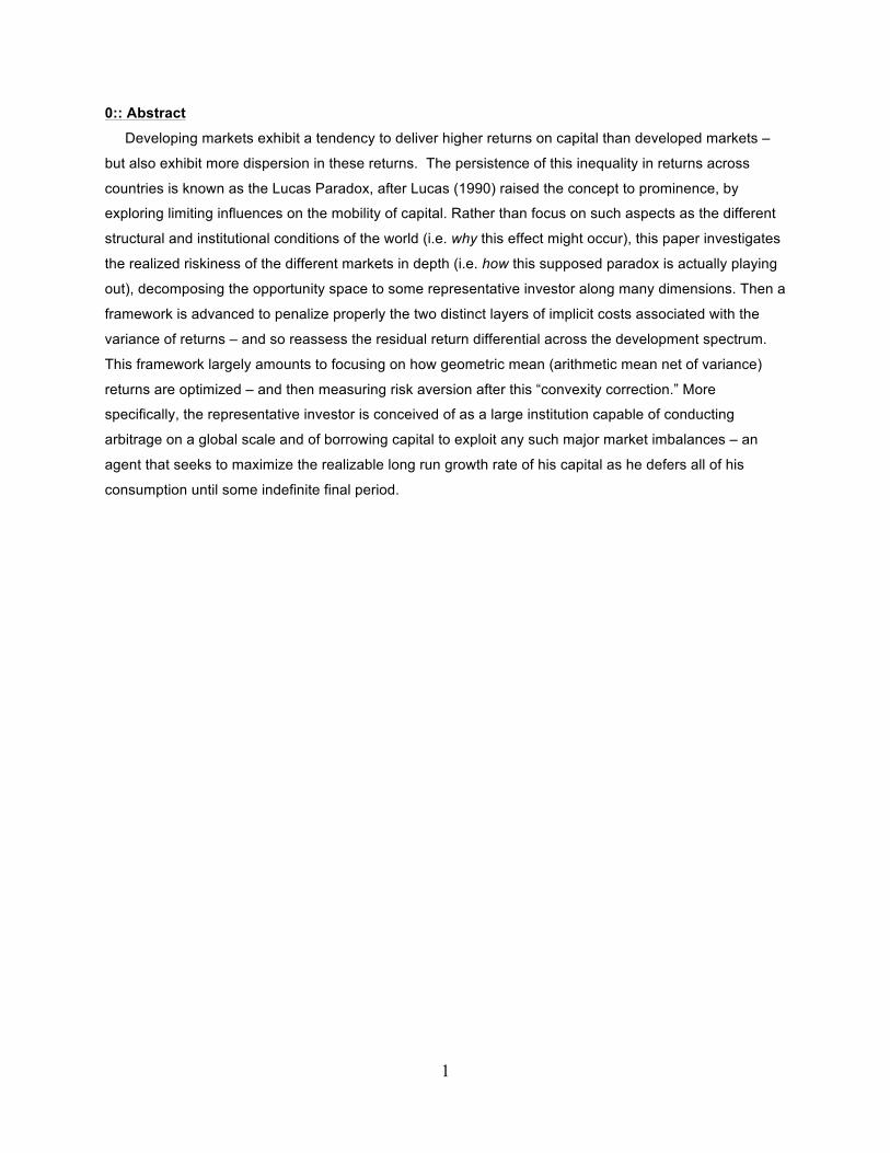
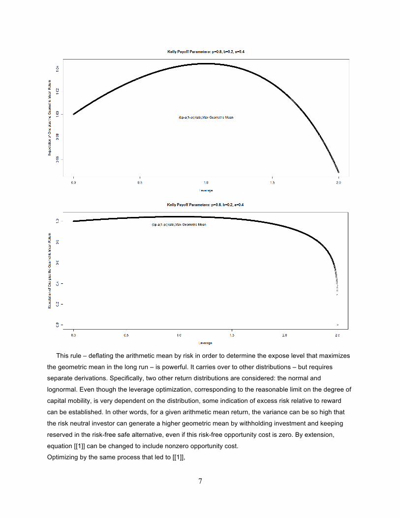
beyond this threshold. If instead the investor faces parameters with p=0.8, b=0.2, and a=0.4, then

xoptimum=0.8/0.4-0.2/0.2=1. If he sets x=1.745172, he will just breakeven.

For the first case, the realizable gains are displayed, first with leverage somewhat near the optimum and

then over the full range, assuming zero opportunity cost.

6

For the second case, the realizable gains are displayed, first with leverage somewhat near the optimum

and then over the full range, assuming zero opportunity cost.

7

This rule – deflating the arithmetic mean by risk in order to determine the expose level that maximizes

the geometric mean in the long run – is powerful. It carries over to other distributions – but requires

separate derivations. Specifically, two other return distributions are considered: the normal and

lognormal. Even though the leverage optimization, corresponding to the reasonable limit on the degree of

capital mobility, is very dependent on the distribution, some indication of excess risk relative to reward

can be established. In other words, for a given arithmetic mean return, the variance can be so high that

the risk neutral investor can generate a higher geometric mean by withholding investment and keeping

reserved in the risk-free safe alternative, even if this risk-free opportunity cost is zero. By extension,

equation [[1]] can be changed to include nonzero opportunity cost.

Optimizing by the same process that led to [[1]],

8

y=(1+bx-r(x-1))p(1-ax-r(x-1))1-p

results in

xoptimum=(1+r)[(p(b-r)-(1-p)(a+r))/((b-r)(a+r))]

[[1b]]

xoptimum=(1+r)[p/(a+r)-(1-p)/(b-r)]=p[(1+r)/(a+r)]-(1-p)[(1+r)/(b-r)]

xoptimum=[(pb-(1-p)a)-r]/[(b-r)(a+r)/(1+r)]

It can be deduced that having a high arithmetic mean is more important when opportunity cost is higher,

although the correspondence is not direct, since xoptimum shrinks rapidly as r approaches b. However, the

relationship between the evolution of opportunity cost and the evolution of mean returns will not be

focused on. Rather, for many purposes, a realistic opportunity cost around 5% (E[r]=0.05) will be

considered as some long run steady state level, matching up closely to the median one year Treasury

rate since the 1950s.

Next the focus shifts from the simple discrete distribution to the continuous case. The log-normal

distribution has the same two parameters for central tendency and dispersion, but µ denotes the

geometric mean, not the arithmetic mean; the variance is also different than its regular counterpart.

Importantly, lognormal distributions are positively skewed, since returns are bounded by -1 on the

downside but can theoretically approach infinity on the upside. Formally, Y is lognormal if

lnY~N(µ,σ2)

In the case of returns,

r=-1+Y=-1+eN(µ,σ2)

The moments for the returns are transformed.

ArithmeticMean[r]=eµ+0.5*σ^2-1

Median[r]=GeometricMean[r]=eµ-1

Var[r]=(e2µ+σ^2)*(eσ^2-1)=(ArithmeticMean[r])2(eσ^2-1)

Thus, the mean/variance ratio after the log transform yields a different relationship.

L=ArithmeticMean[r]/Var[r]=(eµ+0.5*σ^2- 1)/[(e2µ+σ^2)*(eσ^2-1)]

=1/[ArithmeticMean[r](eσ^2-1)]

[[3]]

Since L varies inversely with µ in this lognormal case, the Merton Rule does not carry over well, even

though the positive skew inherent in the lognormal distribution should boost the true L; rather, the positive

skew complicates the estimation process. It turns out that having this positive asymmetry inherent in the

log-normal return distribution makes a meaningful difference in the mean/variance ratio – and

consequently the estimation of optimal leverage. Specifically, the lognormal variance overstates the true

downside risk relative to the upside. The distortion in the mean/variance ratio switching from the normal to

the log-normal for a host of selected parameters can best be handled by simulation. After calculating the

actual geometric mean using the code in the appendix, under various leverage levels, with a large

number of random lognormal returns resampled a very large number of times, it seems at first that it is

9

possible to generate a higher geometric mean than at L=1 when L>1, but eventually the risk of ruin is

realized for a nontrivial variance. By the definition of the lognormal support, rmin=0+ ε, where ε is some

trivially small positive number, so a hypothetical return of -0.9999 with L=1.2 would result in an effective

return of (1.2)*(-0.9999) = -1.1988 < -1. Any investment generating a return less than or equal to -1 is

ruined and ends up with a final level of capital of zero. To follow through on this principle more rigidly, if

we apply a linear transformation to the lognormal, we get an interesting result.

lnY~N(µ,σ2)

b*Y+c=b*eN(µ,σ2)+c

b*Y+c=eln(b)+N(µ,σ2)+c

b*Y+c=eN(µ+ln(b),σ2)+c

The scaling (b) and shifting (c) actually both result in shifting. For the effect of leverage, since (for the

basic case of L=2) some arithmetic yields (1+r)*2-(2-1)=1+2r,

b=L

c=-(L-1)

L*Y-(L-1)=L*(Y-1)+1=eN(µ+ln(L),σ2)-(L-1)

Thus, this leveraged distribution has an arithmetic mean shifted by

∆µ=ln(L)-L+1

[[4]]

d(∆µ)/dL=1/L-1

If L=1, then

∆µ=0, d(∆µ)/dL=0

However, we are interested in optimizing the geometric mean, not the arithmetic mean. We know that the

former is less than the latter in every instance with positive variance. But it is difficult to estimate the

geometric mean here, since the leveraged distribution is no longer lognormal. That being said, as L

increases so does the volatility drag (the gap between the arithmetic and geometric means), so the

optimal L would logically be below 1, since above that there would be further drag on a lower arithmetic

mean.

µ>g

The normal approximation of the geometric mean (g=µ-0.5*σ2) holds up loosely in the lognormal case, so

if L>1

∆µ>∆g, where ∆µ<0

Since the adjustment costs, which are indefinite generally and conceivably higher in poorer and less open

regions, are assumed to be nontrivial, the pure-form Ito calculus, over extremely short time periods,

utilized to obtain the Merton Rule does not hold. Next, a derivation is performed to estimate Loptimum with

minimal constraints on the functional form of the return distribution. Ultimately, even after the fact, it is not

clear what the optimal leverage is exactly; the true return distribution does not have to match perfectly

with any parametric probability density function.

10

Regardless of the parametric form of the distribution, the rule of maximizing expected utility holds in all

cases.

U≠E[1+r]

U=E[ln(1+r)]

[[5]]

So, moderate risk aversion (logarithmic utility) in the one period case corresponds exactly to risk

neutrality (linear utility) in the multi-period case. For any distribution of returns, maximizing the geometric

mean is tantamount to maximizing final wealth,

max{Π1:T(1+rt)}

=max{Σ1:T(ln(1+rt))}

=max{E[ln(1+r)]}

[[6]]

For r2<1,

max{E[U]}

=max{E[ln(1+r)]}

The Mercator series expansion converges for r2<1.

=max{E[r-r2/2+r3/3-r4/4+r5/5+…]}

≈max{E[r-r2/2]}

=max{E[r(1-r/2)]}

The expectation of the product minus the product of the expectation defines the covariance.

=max{E[r]E[1-r/2]+Cov[r,1-r/2]

=max[E(r)E[1-r/2]-Var[r]/2}

Allocation decision: buy X of one security with zero risk-free rate (rf=0) opportunity cost, so L=X/K

E[r]=Lµ

Var[r]=(Lσ)2

max{E[r]E[1-r/2]-Var[r]/2}=>

Set the derivative to zero.

0=d[Lµ(1-Lµ/2)-L2σ2/2]/dL

0=µ-Lµ2-Lσ2

L= µ/(µ2+σ2)

For sufficiently small µ, where the Mercator series truncation is most representative,

Loptimum= µ/σ2

[[7]]

Borrowing from earlier work done by Merton, a simpler derivation can be examined for the normal

distribution. In this normal setting, a special scaling property results, derived via Ito’s Lemma as the

parameters approach zero.

11

ln(KT)-ln(K0)=L[(µ-Lσ2/2)T+σt1/2Z]

Here Z represents a standard normal shock.

Z~N(0,1)

For one (infinitesimal) step forward (T=1):

g=Lµ-(Lσ)2/2

g'=0=µ-Lσ2

Loptimum=µ/σ2

[[8]]

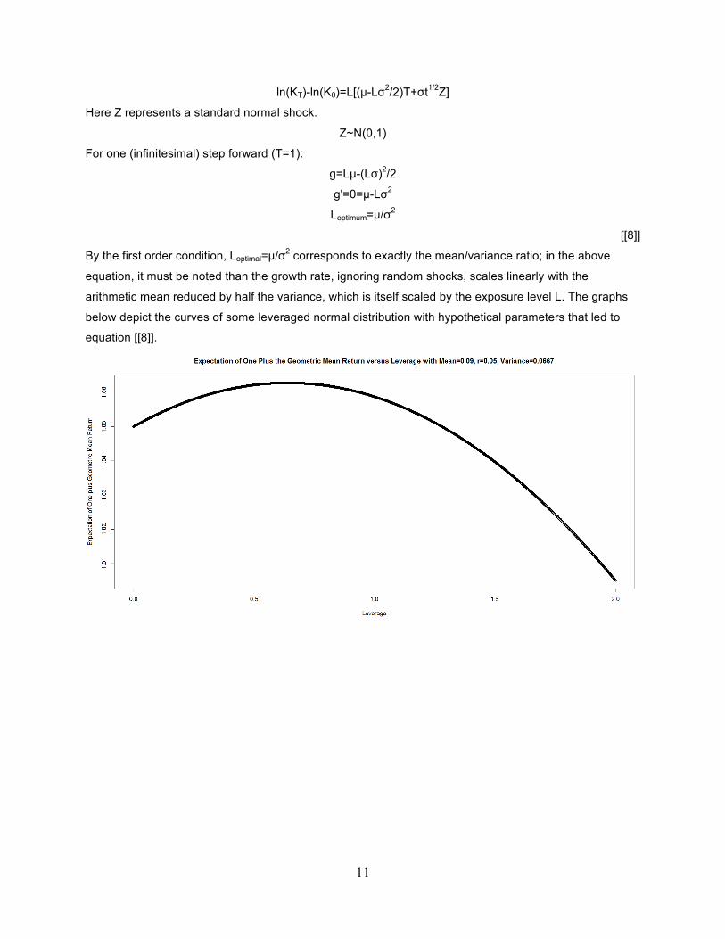
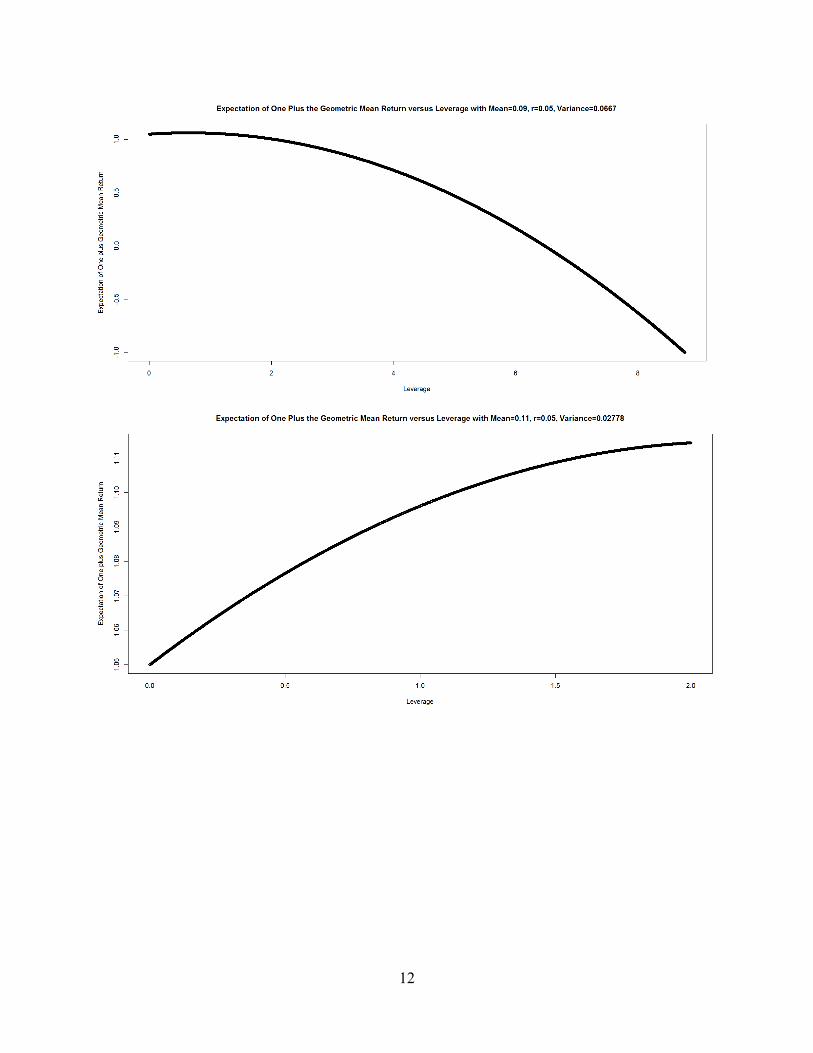
By the first order condition, Loptimal=µ/σ2 corresponds to exactly the mean/variance ratio; in the above

equation, it must be noted than the growth rate, ignoring random shocks, scales linearly with the

arithmetic mean reduced by half the variance, which is itself scaled by the exposure level L. The graphs

below depict the curves of some leveraged normal distribution with hypothetical parameters that led to

equation [[8]].

12

13

All of the above extensions require a sufficiently large amount of data in order for each one to be

accounted for appropriately with precision. Centuries of data would yield more sound estimations.

However, these extensions nonetheless serve to buttress the key insight here: that the arithmetic mean

returns must be deflated by some measure of risk (roughly corresponding to the variance), in order to

determine the optimal allocation for maximizing the geometric mean of returns, thereby implying the

representative agent is truly a rational (yet possibly risk-averse) utility-maximizer. The specific method of

penalizing instability and framing the risk-deflator will lead us to assess more appropriate estimates of

genuine risk aversion preventing capital from flowing to poor countries, thereby retarding development.

After calibrating these allocations based on the arithmetic mean reduced by the risk deflator, then the

condition of parity of the rescaled geometric returns will be robustly tested. Specifically, these rescaled

geometric mean returns will be regressed on lnGDPpc, with the null hypothesis being a slope of zero and

the plausible alternative being a slope less than zero, reflecting a certain degree of genuine risk aversion.

More generally, for any distribution of returns, equation [[6]] can be extended

maxL{Σ1:T(ln(1+Lrt))}=>

0=Σ1:T(L/(1+Lrt))

[[0.3]]

This condition can be handled by simulation for any distribution, parametric or not. For each country –

and for all countries together – a resampling procedure can be conducted to determine the optimal

leverage (L0). This estimation process allows for nonparametric optimization, given that the true

distribution of returns is most likely not exactly lognormal since negative returns are so uncommon;

however, the empirical distribution can also be matched to the lognormal, for the sake of conformity.

14

So before risk aversion can be accounted for, the primary layer of the cost of risk, which can be called

sensitivity, must be captured. Everyone is sensitive to risk because, ceteris paribus, it reduces the

geometric mean return, which the risk neutral agent attempts to maximize. Since all risky markets exhibit

nonzero variance, it has been established that Loptimum is finite – and so capital mobility of all agents

collectively is finite. But what is the true limit on capital mobility? There are two important thresholds: the

soft limit, which reflects Loptimum under various assumptions about the distribution of returns and the

opportunity cost, and the hard limit, which reflects the maximum leverage Lmax that can be applied without

going bankrupt and being ruined. The hard limit can be more explicitly determined, although it is

statistically less stable since it depends on one outlier, the minimum return.

Lrmin-(L-1)rf=-1

Lmax=-(1+rf)/(rmin-rf)-ε

[[10]]

Here, ε is some trivially small positive number approaching zero. In the entire span of all observations

across countries and years, the minimum returns were rare and not severe: for alpha=0.3, rmin= -0.04591,

corresponding to Lmax=10.947999 with given opportunity cost rf=0.05, and Lmax=21.781999 with rf=0; for

alpha=0.4, rmin= -0.039431, Lmax=11.741 with rf=0.05, and Lmax=25.360999 with rf=0. Indeed, this hard

boundary, while explicitly calculable, is very unstable and dependent on the assumptions of the

distribution of returns and opportunity cost.

Aversion

Behavioral economists have contended frequently that the pain of losing one dollar is much greater in

magnitude than the joy of winning one dollar. And there absolutely exist psychological costs of losing –

the deadweight cost of feeling like a loser and other such emotional forces that might drag on future

productivity. These complications are part of why the representative agent considered here should be

thought of as a large institution with a completely negligible current consumption requirement and is

capable of allocating efficiently and investing anywhere in the world when an opportunity is recognized.

Moreover, the investor is not very constrained by the credit markets unless his effective leverage greatly

exceeds one (if L*>>1, then rcredit>>rf). The fundamental condition for risk aversion follows.

U(E[K])>E[U(K)]

This essential tenet of risk aversion holds in all contexts, where capital or consumption is considered. On

a concrete level, it is obvious that utility should exhibit diminishing marginal returns to wealth. If the

representative agent scales his consumption positively with his current wealth level, then – since

everyone must consume some set of necessities to survive – if wealth drops below some critical level

corresponding to the poverty line, then the pain of losing would become overwhelming. If instead the

agent’s wealth level is sufficiently high, then there is a negative externality to losing money – namely, that

this agent would either get fired from his job as a portfolio manager or would gradually lose his client

base. In order to deal with these nuances in a consistent fashion, Constant Relative Risk Aversion

15

(CRRA) – also known as iso-elastic – preferences will be adopted; this functional form possesses the

advantage of being indifferent to the frame of reference that is initial wealth, although it was argued above

that approaching ruin or poverty might escalate the aversion. A pair of CRRA utility functions is proposed.

Constant Relative Risk Aversion (CRRA):

U1=(K1-γ -1)/(1-γ), where γ=-K*(d2U1/dK2)/(dU1/dK) and γ is constant

Constant Absolute Risk Aversion (CARA):

U2=(1-Γ)/Γ*(K/(1-Γ))Γ, where Γ=-(d2U1/dK2)/(dU1/dK) and Γ is constant

Intermediate consumption is restricted to zero, reflecting the institutional nature of the representative

investor who simply wants to maximizes capital in some indefinite final period.

CT=KT, where Ct≠T=0

[[0.2]]

Risk neutrality for the first equation corresponds to zero (γ=0), whereas for the second equation it

corresponds to one (Γ=1). Both equations are special cases of the hyperbolic form. More generally, to

frame equation [[11]] properly, a baseline on recursive preferences is sought, where zero utility is derived

from intermediate consumption, with Epstein-Zin parameters restricted to the limits of their domains.

Ut=[(1-β)Ctρ+β(E[Ut

α])ρ/α]1/ρ

Set β=1,α=1,ρ=0.

Ut=E[Ut]

The key insight here is that there are two distinct layers to risk that absolutely must be accounted for

separately. There are observable degrees of variance (as well as skew and kurtosis) that drag on long

run compounded growth, and function as deflating factors on the arithmetic mean when the agent is

venturing to optimize his geometric mean. If the investor simply compares the arithmetic means of various

countries against their respective logarithmic GDP per capita, then the Lucas Paradox appears to be

dominant. It is here where this paper departs from that of Henriksen (2014). If we simply regressed

arithmetic mean returns on log GDPpc, there would appear to be massive risk aversion in the global

capital markets, which might only be justified by the structural incongruity of poor countries versus rich

ones, such as monopolies that actively retard foreign competition or government-supported capital

controls that both reflect a lack of openness – factors that critically might result in sufficiently high

adjustment costs to capital. Only looking at the arithmetic mean returns for each countries would be valid

if and only if the variance of returns were held perpetually at zero, an obviously false condition which only

applies to short-duration government bonds of mature developed countries. These prohibitive adjustment

costs would then deprive the representative agent of the opportunity to reallocate periodically, forcing him

to make a major fixed capital commitment in just one period and basically stick with it over a long

duration; in other words, lack of openness would generate a new and analytically problematic

idiosyncratic risk factor reflecting a lack of liquidity.

16

3:: Methods

The true degree of risk aversion is difficult to capture, still more difficult to capture without examining

consumption patterns. Essentially, the goal is in framing how much money is being left on the table, under

two conditions – fully credit constrained investors (L=1) and partially credit constrained (L=2). Both

conditions limit the investor to being less exposed than the estimation of optimal exposure presented in

the results section, but a leverage of two is not excessive and would hold up in the future if the worst case

loss increases significantly. Two derivations are proposed in this section. The first ends up being a

nonlinear function of the mean/variance relationship, the second a linear one. Even though the focus of

this paper is on long run geometric mean return maximization, for convenience only one step forward will

be analyzed – a practice valid only under serial independence of the returns, a property also known as

“partial myopia.” So, while developing countries might be converging to developed ones, thereby reducing

their variance and mean returns over time, the historically observable data will be assumed to hold going

forward, representing a sample from some static governing distribution. For a reduced-form baseline

version of the relative risk aversion parameter independent of inter-temporal consumption requirements,

with a derivation based in part on (Jacquier 2011), let

E[Kt]=K0(1+g)t

1+g=eLµ-0.5*(L*σ)^2-(L-1)r

For simplicity, set

K0=1, t=1

Then solve the objective function.

maxL{E[U(K(L))]}=>

0=E[U'(K)*K'(L)]

The covariance is the expectation of the product minus the product of the expectations.

0=Cov[U'(K),K'(L)]+E[U'(K)]*E[K'(L)]

Stein’s Lemma is used to decompose the covariance further.

0=E[U''(K)]*E[K'(L)]*Cov[K(L),K'(L)]+E[U'(K)]*E[K'(L)]

γ≡-E[U''(K)]/E[U'(K)]=1/Cov[K(L),K'(L)]

[[12]]

Cov[K(L),K'(L)]=βK',K*σ2K

βK',K=∆K'/∆K=K''/K'

=[(eLµ-0.5*(Lσ)^2-(L-1)r)*((µ-r-Lσ2)2-σ2]/[(eLµ-0.5*(Lσ)^2-(L-1)r)*(µ-r-Lσ2)]

=((µ-r-Lσ2)2-σ2)/(µ-r-Lσ2)

=(µ-r-Lσ2)-σ2(µ-r-Lσ2)-1

=>Cov[K(L),K'(L)]=σ2((µ-r-Lσ2)-σ2(µ-r-Lσ2)-1)

=>γ=1/[σ2((µ-r-Lσ2)-σ2(µ-r-Lσ2)-1)]

=((µ-r)/σ2-L)/((µ-r-Lσ2)2-σ2)

[[13]]

17

γ L=(µ-r)/σ^2=γ(µ-r)/σ^2=0

γ1=((µ-r)/σ2-1)/((µ-r-σ2)2-σ2)

[[14]]

Then, to assess the absolute risk aversion level, a derivation based in part on Sandmo (1970) is

presented. Here, eta is the risk premium (the difference between the expected final consumption and the

certainty-equivalent level) and h is the approximation for standard deviation of the risky outcome.

Γ=2η/h2

h2=(Lσ)2

η=[Lµ-0.5*(Lσ)2-(L-1)r]-r

Γ=2((µ-r)/σ2)/L-1

[[15]]

ΓL=1,r=0=2µ/σ2-1

[[16]]

ΓL=(µ-r)/σ^2=1

Risk aversion metrics can be computed for each country or each portfolio – and then measured across

the factor that is used to construct the portfolio: GDPpc, GDPpw, and ECI. Based on the various

derivations of optimal leverage in the risk sensitivity segment of section two, the mean/variance ratio

functions as a good rule of thumb but is not perfect, other than for cases with very small variance.

Consequently, for practical purposes, L should be set somewhere between one and the optimal

(1<L*<Loptimal), depending on the confidence that the investor has in the estimation of the true return

distribution. Given the overall distribution of all country-year observations, this modification corresponds

to setting the effective leverage at one and then gearing it up to two (L*=1,2). However, this minimalist

estimation of risk aversion is ascertainable without any consumption data; this estimation is very

important to establish before consumption is considered. Consumption is the next dimension to

investigate, for the explicit purpose of establishing some arbitrage-free baseline on the degree of risk

aversion. In other words, this procedure captures the first layer of the implicit costs of risk, and the

covariance of consumption with returns forms the second layer, firmly on top of the first. The evaluation of

this second layer of implicit costs, conducted via the framework of Epstein-Zin recursive preference, will

be left to other research projects. But it is sufficient to note that, if the representative investor prefers to

consume anything in the time in between the first and final periods (valid for virtually all agents yet trivial

for the largest ones), then his risk aversion will be higher than this reduced-form base metric. However,

since the effective leverage (L*) applied to each country is unobservable, different key values are tested

from 1 to 2. However, all of the effort to configure different leverage levels should be constrained by the

accounting identity that the net borrowing and lending must balance out, satisfying the universal clearing-

condition that aggregate leverage is pinned to unity (E[L*]≡1). In other words, it is inconceivable that the

aggregated effective leverage for any group of countries should deviate indefinitely from unity. Moreover,

maintaining a yearly rebalanced constant leverage different from one (L*≠1) is only feasible under trivial

18

adjustment costs, which are indefinitely high when aggregate physical capital is considered, especially for

poor countries that might lack open capital markets (as Lucas points out in detail in his original paper). It

should be noted that the relative risk aversion metric is nonlinear transform of the mean/variance ratio,

whereas the absolute risk aversion metric is a linear transform.

In spite of all the mathematical complications, there is sufficient evidence that Loptimum>1, even with

nontrivial adjustment costs and transaction costs – mainly because the left tail of the return distribution is

so limited.

4:: Results

It can clearly be seen that the variance of the returns to capital in poor countries is higher than in rich

countries. Some countries, mainly those associated with the CIS and formerly under the Soviet system,

lack sufficient data to be analyzed with the appropriate precision. Since only 25 years have elapsed since

their respective time series began, there is the potential for small sample bias, which is problematic in

general and crucially so in this risk related context. It is commonly accepted that the number of

observations exceed T>30 for this small sample bias to become adequately reduced in significance.

If the estimate for the genuine degree of risk aversion is sufficiently greater than zero or one,

corresponding to risk neutrality, then the Lucas Paradox survives. Moreover, if risk aversion is high in this

context, then the implications are very interesting. For one thing, high risk aversion might indicate an

arbitrage opportunity is not being exploited, but this conclusion might be wishful thinking. For one thing,

the whole estimation process implies than the brief (in statistical terms) historical sample yields the exact

true parameters governing the future distribution of returns, which is a weak assumption; further work

might endeavor to incorporate Bayesian updating to the estimation process for recovering these true

parameters for the marginal distributions, but this complexity is outside the scope of this paper. Before the

actual degree of risk aversion can be properly assessed, the mean/variance ratio must be evaluated for

every country over different time periods, under varied assumptions. If the ratio is below one

(Loptimum≈µ/σ2<1), which is not the case except for a few countries, then there is some degree of excess

variance – since the risk-neutral geometric mean return maximizer will withhold investment and keep

some portion of his capital (1-Loptimum) in the debt market.

Here the primary relationship is displayed with the arithmetic mean returns for each country unadjusted

for variance.

19

20

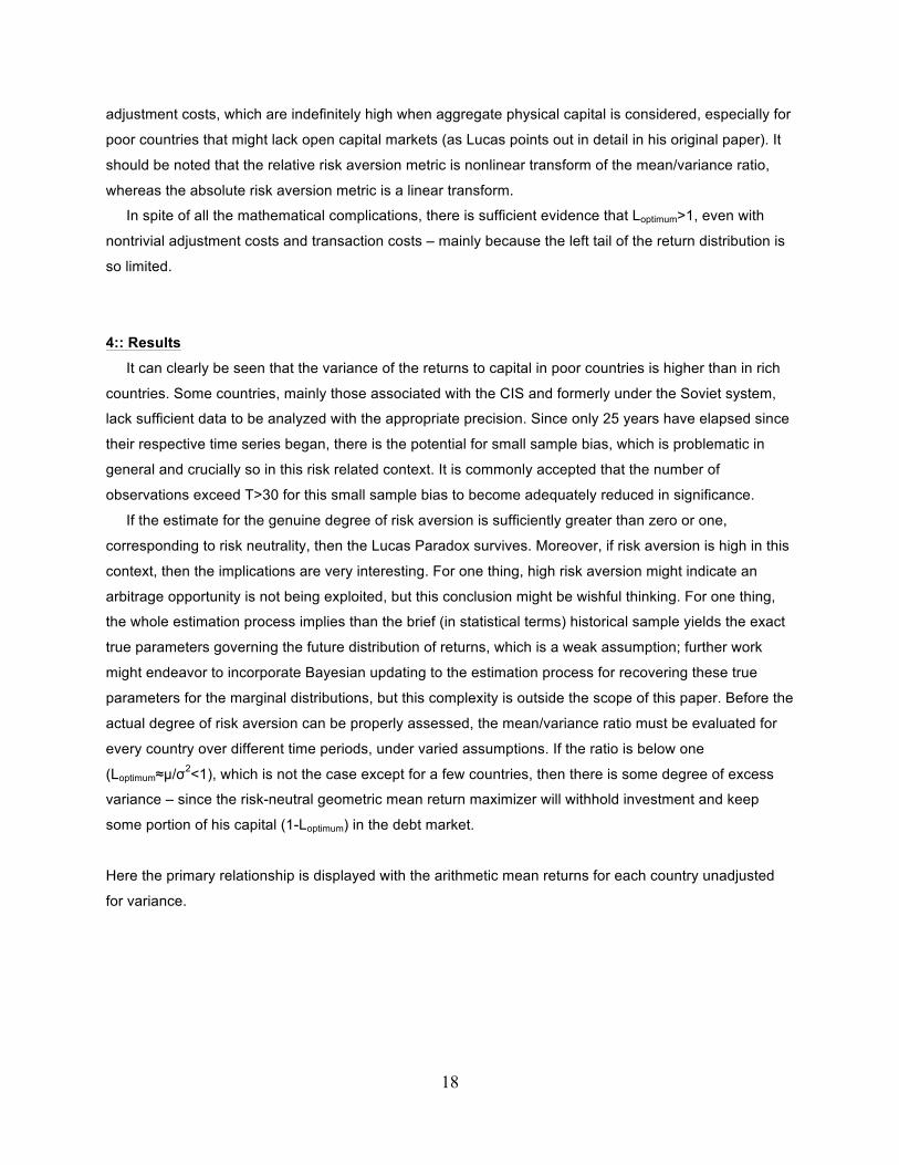
However, while the arithmetic mean return decreases with logarithmic income per capita, the variance

decreases too.

21

This result is intuitive and consistent with the most fundamental principle of efficiency in capital markets –

generating a higher reward requires taking on more risk. But what is the relative rate of change in mean

against variance? In other words, as the arithmetic mean return decreases as income increases, does the

variance decrease faster? In order to assess this question, the individual slopes will be rescaled. The

process of dividing the slopes by the intercepts, all of which having a p-value less than 0.05, results in the

following relative values.

Slope/Intercept Regression of Return Mean on

Log Income Per Capita

Regression of Return Variance

on Log Income Per Capita

1950-2011 -0.08866 -0.10172

1970-2011 -0.073011 -0.098875

22

1990-2011 -0.055206 -0.096154

Since the magnitudes of the values in the first column are all smaller than the magnitude of value in the

second column, the variance is decreasing faster than the mean as income increases, on a relative basis.

However, the magnitudes of the values in the first column are decreasing faster than the magnitudes of

the values of the second column over time. The implication of this observation, tentatively, is that, even if

there is some convergence in the mean returns of poor and rich countries over time, the risk in poor

countries remains persistently higher in the poor countries. Moreover, there is a limit to the extent to

which the means can converge if the variance does not also converge. This limit is important, albeit hard

to measure since the optimal leverage (and corresponding capacity for capital mobility) is somewhat

ambiguous dependent on the true return distribution, which does not have to be stationary. Now the same

relationship is reassessed using the geometric mean return. In the following tables, B denotes the slope

estimate. The slopes are more statistically significant than in the prior regressions with the arithmetic

means, with most having p-values less than 0.01.

B::µG:lnGDPpc 1950-2011 1970-2011 1990-2011

alpha=0.2 -0.03134 -0.01731 -0.00733

alpha=0.3 -0.04646 -0.02518 -0.01053

alpha=0.4 -0.06140 -0.03289 -0.01366

alpha=0.5 -0.07620 -0.04046 -0.01673

The elasticity of returns with respect to GDP per capita, under four different assumptions for the fixed

alpha (the invariant elasticity of GDP with respect to capital), over three different time frames

B::µG:lnGDPpw 1950-2011 1970-2011 1990-2011

alpha=0.2 -0.02032 -0.02088 -0.00815

alpha=0.3 -0.02994 -0.03079 -0.01173

alpha=0.4 -0.03952 -0.04058 -0.01525

alpha=0.5 -0.04907 -0.05027 -0.01873

The elasticity of returns with respect to GDP per worker, under four different assumptions for the fixed

alpha (the invariant elasticity of GDP with respect to capital), over three different time frames

B::ln(1+µG):lnGDPpc 1950-2011 1970-2011 1990-2011

alpha=0.2 -0.02842 -0.01525 -0.00664

alpha=0.3 -0.03968 -0.02071 -0.00897

alpha=0.4 -0.04961 -0.02541 -0.01101

alpha=0.5 -0.05848 -0.02952 -0.01282

23

B::ln(1+µG):lnGDPpw 1950-2011 1970-2011 1990-2011

alpha=0.2 -0.01926 -0.01872 -0.00737

alpha=0.3 -0.02713 -0.02592 -0.00999

alpha=0.4 -0.03431 -0.03226 -0.01228

alpha=0.5 -0.04089 -0.03789 -0.01432

The correlation drops from an R2~0.3 to ~0.05, moving from the 1950-2011 period to the periods starting

in 1970 and 1990. Moreover, using geometric means in the regression instead of arithmetic means as the

dependent variable results in a lower p-value for the slope estimate B; with arithmetic means it is

significant at the 5% level, and with geometric means it is significant at the 1% level.

The effect of poorer countries generating higher geometric mean returns is now tested for robustness by

substituting a completely distinct metric, the Economic Complexity Index (ECI), for logarithmic income.

The ECI is a structural measure that averages together all of a country’s revealed comparative

advantages, using the Balassa definition, in the export market for goods.

B::µG:ECI 1970-2011 1990-2011

alpha=0.2 -0.02230 -0.01680

alpha=0.3 -0.03290 -0.02500

alpha=0.4 -0.04340 -0.03320

alpha=0.5 -0.05380 -0.04130

B::ln(1+µG):ECI 1970-2011 1990-2011

alpha=0.2 -0.01990 -0.01510

alpha=0.3 -0.02760 -0.02110

alpha=0.4 -0.03430 -0.02650

alpha=0.5 -0.04030 -0.03120

The ECI, representing the standard score for a structural model of the diversity and exclusivity of each

country’s product space, is the distinct substitute for lnGDPpc and lnGDPpw. The consistency between

the two types of explanatory variables confirms that there is a genuine development effect on capital

returns.

Next, the direct reward-risk association is displayed, with B0 being the intercept and B1 the slope.

B0::µG:ln(1+σ2) 1950-2011 1970-2011 1990-2011

alpha=0.2 0.04670 0.05720 0.04100

alpha=0.3 0.08790 0.10400 0.08060

alpha=0.4 0.12800 0.15000 0.12000

alpha=0.5 0.16700 0.19600 0.15900

24

B1::µG:ln(1+σ2) 1950-2011 1970-2011 1990-2011

alpha=0.2 14.26270 8.52410 13.55900

alpha=0.3 12.23260 7.34500 11.59700

alpha=0.4 11.32500 6.87000 10.68000

alpha=0.5 10.87000 6.66200 10.18000

Geometric mean returns at L=1 versus the logarithmic transform of variance, to allow for preferences to

reveal diminishing marginal gains to taking on more risk

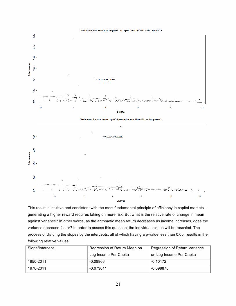
Taking a step back, the distributions of returns are displayed without the income dimension.

Next the geometric mean of returns plus one, with a random draw from the above histogram of all

country-year returns, is displayed. Since the distribution is so favorable, with a small left tail and large

right tail, the optimal leverage is very high, but the maximum leverage, at which bankruptcy is reached, is

only one extremely small increment higher; this extremely rapid turn from optimal to failure can barely be

seen on the graph below, with the apparent right hand endpoint turning down. So, perhaps ironically,

optimizing the exposure to this highly favorable distribution of returns is dangerous. If this aggregate

empirical distribution is discretized to the Kelly case reflected in equation [[1]], then

p=0.99864,b=0.12526, and a=0.01746. (The R script for this curve is straightforward and listed in the

appendix.)

25

The key limit here is right below Lmax=10.948; due to the favorability of the distribution, perhaps

paradoxically, this curve dangerously falls off a cliff, meaning that the soft limit ([[0.3]], [[1b]]) of the

optimal leverage is smaller than the hard limit ([[10]]). In other words, the exception is the rule here; if the

rarest outlier, the minimum return, dictates the effective limit on the capacity of capital mobility. Even

though the minimum observed return is less than 5%, there is nothing preventing the minimum from being

more extreme in the future; philosophically, especially given the limited time period of the observations,

the biggest loss is always on the horizon. Some extreme shock like a natural disaster could destroy a

huge portion of the capital stock in a small poor country, thereby increasing the depreciation rate close to,

say, 50%, which is a critical level for the L=2 case. Or a political regime shift to a command economy

might compromise the investor’s capital commitment to one country. These natural disaster and political

revolution type of shocks can and do happen; on a portfolio level, these events will have a muted impact,

but the risk is not eliminated – the probability is just reduced, but not to zero (Pr[catastrophe]>0). The

optimal leverage is clearly greater than one, but pushing it to the apparent limit is precarious;

overshooting is deadly. So all countries together permit some level of borrowing, but it is not clear that the

representative investor would borrow more to invest in the poor countries, given the drag on leveraged

returns from the high variance. In fact, it is the other way around, as long as interest rates are not too

high; with low interest rates, rich countries can be levered somewhat more highly than poor countries.

26

27

It is obvious that the left tail is not “fat.” Negative returns are rare and small. The minimum return was less

than 5%. If an investor borrowed 8.999 dollars with interest rate of 5%, close to the median opportunity

cost over the entire 1950-2011 period based on the one-year US Treasury rate, he would have survived

the 5% loss just barely without going bankrupt. Moreover, the distribution is positively skewed, so all the

approximations relying on manipulating the normal distribution and restricting the variance to be small

should be taken with a grain of salt.

Next, the cross-sectional mean and the cross-sectional variance are displayed. The cross-sectional

variance has decreased over time, indicating some degree of mean return convergence; this converge

has taken place as the cross-sectional mean of returns has decreased over time as well, which weakens

the case for convergence. It should be noted that the paths of both cross-sectional metrics has not been

smooth, and there is no guarantee that the distribution governing returns is stationary.

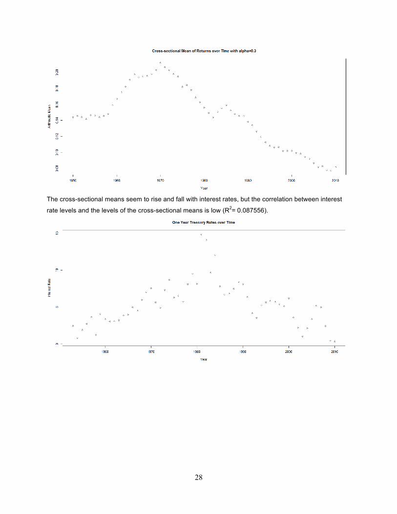
28

The cross-sectional means seem to rise and fall with interest rates, but the correlation between interest

rate levels and the levels of the cross-sectional means is low (R2= 0.087556).

29

Also, mean returns are declining over time as mainly poor countries are added to the PWT, so the case

for opportunity in poor countries is further weakened. Next the rolling time series variance of all countries

over the past 20 years is displayed. Mathematically, if the period of calculation is 20 years, then the

corresponding lag is 10 (20/2), meaning the latest observation reflects the rolling variance 10 years ago. It

should be noted that this rolling variance is not decreasing. This is somewhat surprising considering that

the cross-sectional mean of returns has declined, but it is not inconsistent with the cross-sectional

variance decreasing over time. The decrease in cross-sectional variance combined with increase in the

time series variance indicates that the risk of the middle income countries has increased even as the risk

of the poor countries has somewhat lessened; that being said, the variance of poor countries is still much

higher than the variance of middle income countries, just not as much as it used to be.

30

The null hypothesis of the neoclassical return parity across the world implies a slope of geometric means

against countries’ log GDP per capita to be zero; the Lucas Paradox stipulates that the slope is less than

zero, although Lucas and others failed to make the crucial distinction between arithmetic and geometric

means. This zero-slope null hypothesis implies some type of equilibrium; this equilibrium can take on

either the strong-form or the weak-form.

The strong-form equilibrium implies that inefficiency is quickly exploited as the capacity for capital mobility

is infinite; this condition is simply false. The weak-form equilibrium implies that the inefficiency of high

returns to capital in poor countries due to relative capital scarcity is exploited but not necessarily quickly,

as the capacity for capital mobility is finite and the individual investor’s leverage can only temporarily rise

above one – and as the information about the opportunity space is incomplete and delayed. The weak-

form condition reflects reality but is more difficult to explore, as the precise capacity for capital mobility is

uncertain even if it is definitely finite. In fact, infinite capital mobility (Lmax->∞) is only possible if it is

impossible for any one country-year return observation to be below the opportunity cost threshold (rmin>rf);

this inequality implies that the investor does not go bankrupt but could still generate a negative geometric

mean at a sufficiently high leverage. However, as long as variance is nonzero, the soft limit is below the

hard limit (Loptimum<Lmax), so infinite capital mobility is bogus.

The returns in poor countries are not less correlated to the global opportunity space as a whole, as the

following graphs indicate. So the variances of poor countries are higher without less covariance to

compensate.

31

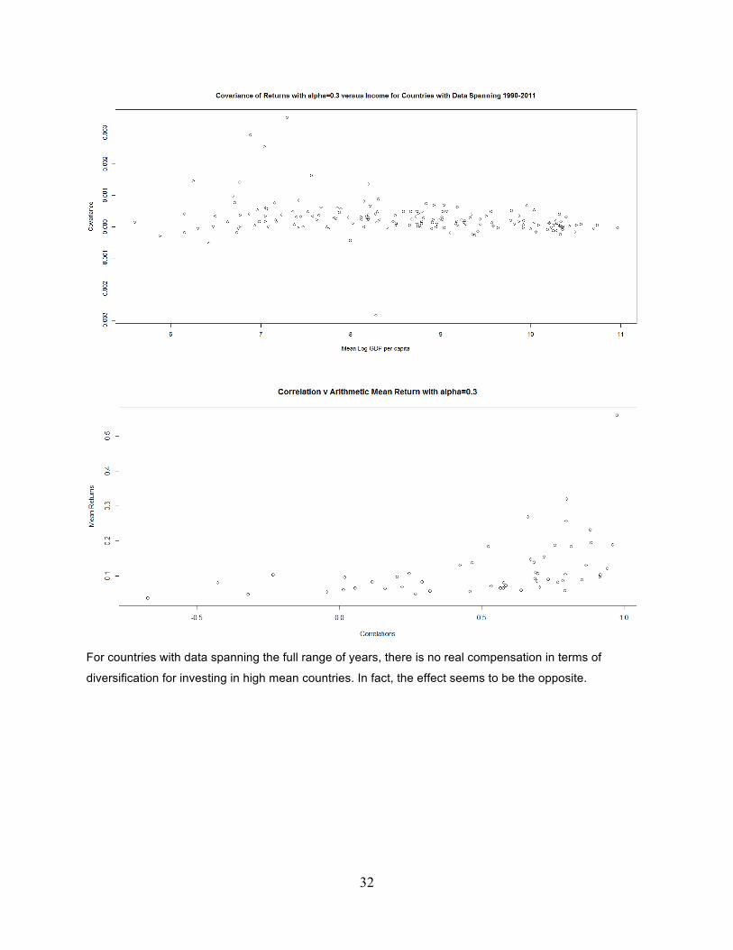
32

For countries with data spanning the full range of years, there is no real compensation in terms of

diversification for investing in high mean countries. In fact, the effect seems to be the opposite.

33

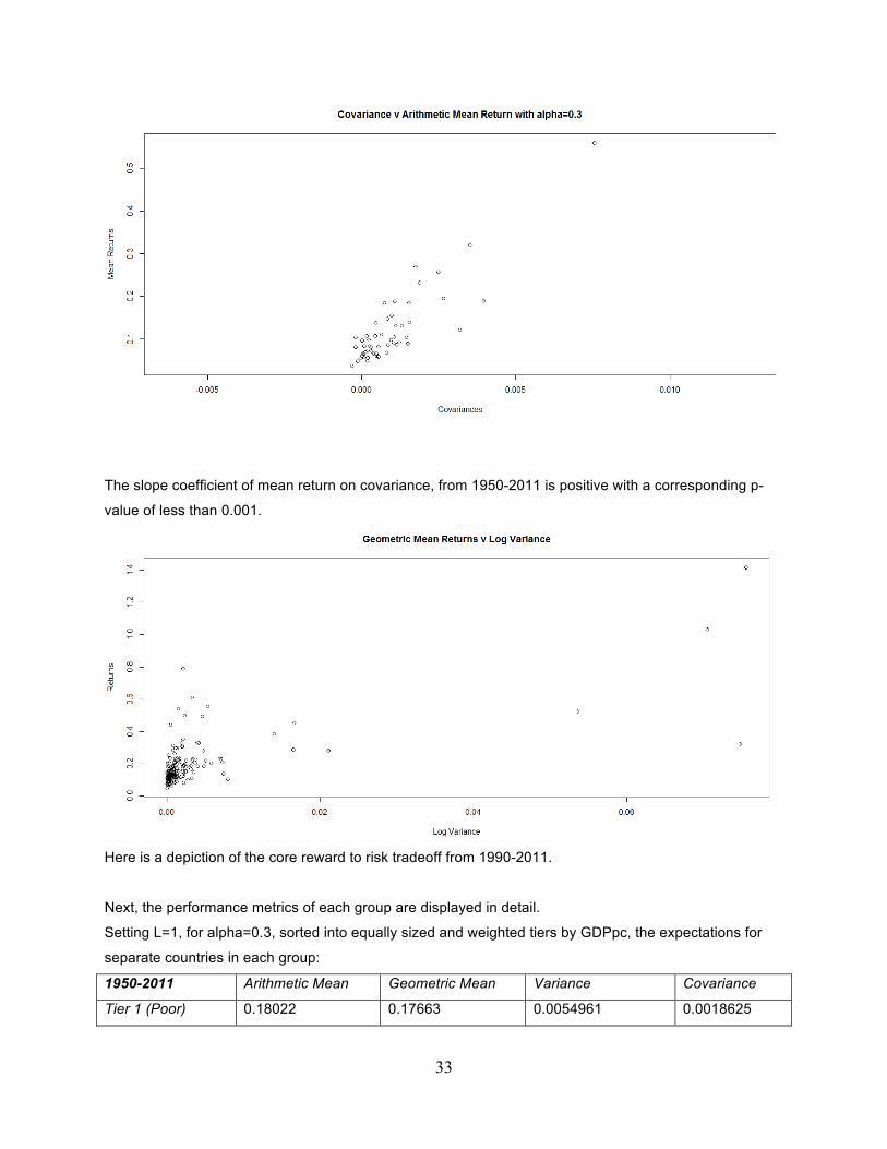
The slope coefficient of mean return on covariance, from 1950-2011 is positive with a corresponding p-

value of less than 0.001.

Here is a depiction of the core reward to risk tradeoff from 1990-2011.

Next, the performance metrics of each group are displayed in detail.

Setting L=1, for alpha=0.3, sorted into equally sized and weighted tiers by GDPpc, the expectations for

separate countries in each group:

1950-2011 Arithmetic Mean Geometric Mean Variance Covariance

Tier 1 (Poor) 0.18022 0.17663 0.0054961 0.0018625

34

Tier 2 (Middle) 0.1123 0.11132 0.0017048 0.00081964

Tier 3 (Rich) 0.067418 0.067248 0.00031898 0.000229

1970-2011 Arithmetic Mean Geometric Mean Variance Covariance

Tier 1 0.17492 0.16916 0.0083312 0.0020928

Tier 2 0.1415 0.13972 0.0027107 0.0010729

Tier 3 0.091978 0.091398 0.0010288 0.00057804

1990-2011 Arithmetic Mean Geometric Mean Variance Covariance

Tier 1 0.11182 0.10985 0.0031074 0.000461

Tier 2 0.1132 0.11199 0.0017115 0.00024305

Tier 3 0.079593 0.079413 0.00033749 0.000097695

Setting L=1, for alpha=0.3, sorted into equally sized and weighted portfolios by GDPpc, the expectations

for combined countries in each group:

1950-2011 Arithmetic Mean Geometric Mean Variance Covariance

Portfolio 1 0.18218 0.1806 0.0027311 0.002321

Portfolio 2 0.1123 0.11191 0.00070232 0.00093918

Portfolio 3 0.067418 0.067335 0.00015729 0.00024534

1970-2011 Arithmetic Mean Geometric Mean Variance Covariance

Portfolio 1 0.17492 0.17292 0.003506 0.0027377

Portfolio 2 0.14247 0.14207 0.00072194 0.0012145

Portfolio 3 0.091978 0.091826 0.00028322 0.00065147

1990-2011 Arithmetic Mean Geometric Mean Variance Covariance

Portfolio 1 0.11182 0.11135 0.00088354 0.000581

Portfolio 2 0.1132 0.11312 0.00015635 0.00024044

Portfolio 3 0.079593 0.079559 0.000065694 0.00010673

For a few developing countries, the GDP data starts one year before data on capital stock is available;

these countries get sorted but the return data point is ignored for that year. Without such countries,

portfolio grouping should indicate identical arithmetic mean returns against the tiered individual country

returns. Then, as long as the countries within each portfolio are not perfectly correlated, the geometric

mean return of the portfolio will exceed that of the tier. The covariance indicates the measure of each

group’s returns relative to the all-country equal-weight average.

35

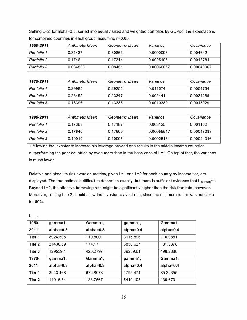
Setting L=2, for alpha=0.3, sorted into equally sized and weighted portfolios by GDPpc, the expectations

for combined countries in each group, assuming rf=0.05:

1950-2011 Arithmetic Mean Geometric Mean Variance Covariance

Portfolio 1 0.31437 0.30863 0.0090098 0.004642

Portfolio 2 0.1746 0.17314 0.0025195 0.0018784

Portfolio 3 0.084835 0.08451 0.00060877 0.00049067

1970-2011 Arithmetic Mean Geometric Mean Variance Covariance

Portfolio 1 0.29985 0.29256 0.011574 0.0054754

Portfolio 2 0.23495 0.23347 0.002441 0.0024289

Portfolio 3 0.13396 0.13338 0.0010389 0.0013029

1990-2011 Arithmetic Mean Geometric Mean Variance Covariance

Portfolio 1 0.17363 0.17187 0.003125 0.001162

Portfolio 2 0.17640 0.17609 0.00055547 0.00048088

Portfolio 3 0.10919 0.10905 0.00025131 0.00021346

+ Allowing the investor to increase his leverage beyond one results in the middle income countries

outperforming the poor countries by even more than in the base case of L=1. On top of that, the variance

is much lower.

Relative and absolute risk aversion metrics, given L=1 and L=2 for each country by income tier, are

displayed. The true optimal is difficult to determine exactly, but there is sufficient evidence that Loptimum>1.

Beyond L=2, the effective borrowing rate might be significantly higher than the risk-free rate, however.

Moreover, limiting L to 2 should allow the investor to avoid ruin, since the minimum return was not close

to -50%.

L=1 ::

1950-

2011

gamma1,

alpha=0.3

Gamma1,

alpha=0.3

gamma1,

alpha=0.4

Gamma1,

alpha=0.4

Tier 1 8924.505 119.8001 3115.896 110.0881

Tier 2 21430.59 174.17 6850.627 181.3378

Tier 3 129539.1 426.2797 39289.61 498.2888

1970-

2011

gamma1,

alpha=0.3

Gamma1,

alpha=0.3

gamma1,

alpha=0.4

Gamma1,

alpha=0.4

Tier 1 3943.468 67.48073 1795.474 85.29355

Tier 2 11016.54 133.7567 5440.103 139.673

36

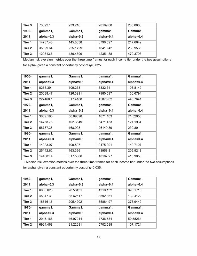
Tier 3 73892.1 233.216 20169.08 283.0688

1990-

2011

gamma1,

alpha=0.3

Gamma1,

alpha=0.3

gamma1,

alpha=0.4

Gamma1,

alpha=0.4

Tier 1 14737.48 145.8038 8796.597 217.6642

Tier 2 35629.64 225.1729 18418.42 238.9565

Tier 3 129513.6 430.4599 42351.88 470.3793

Median risk aversion metrics over the three time frames for each income tier under the two assumptions

for alpha, given a constant opportunity cost of rf=0.025.

1950-

2011

gamma1,

alpha=0.3

Gamma1,

alpha=0.3

gamma1,

alpha=0.4

Gamma1,

alpha=0.4

Tier 1 8288.391 109.233 3332.34 105.8149

Tier 2 25688.47 126.3991 7980.597 160.6794

Tier 3 227468.1 317.4188 45876.02 443.7641

1970-

2011

gamma1,

alpha=0.3

Gamma1,

alpha=0.3

gamma1,

alpha=0.4

Gamma1,

alpha=0.4

Tier 1 3089.196 56.89398 1671.103 71.52058

Tier 2 14758.78 102.3849 6471.433 121.1934

Tier 3 58787.38 168.908 26149.39 239.89

1990-

2011

gamma1,

alpha=0.3

Gamma1,

alpha=0.3

gamma1,

alpha=0.4

Gamma1,

alpha=0.4

Tier 1 14023.97 109.897 9175.091 149.7107

Tier 2 25142.62 163.366 13958.8 205.9218

Tier 3 144681.4 317.5506 48187.27 413.9055

+ Median risk aversion metrics over the three time frames for each income tier under the two assumptions

for alpha, given a constant opportunity cost of rf=0.035.

1950-

2011

gamma1,

alpha=0.3

Gamma1,

alpha=0.3

gamma1,

alpha=0.4

Gamma1,

alpha=0.4

Tier 1 6866.626 98.56431 4319.132 99.51715

Tier 2 45047.3 85.62517 8592.861 132.4122

Tier 3 186161.6 205.4902 55884.97 373.9449

1970-

2011

gamma1,

alpha=0.3

Gamma1,

alpha=0.3

gamma1,

alpha=0.4

Gamma1,

alpha=0.4

Tier 1 2015.168 46.97914 1736.584 59.58264

Tier 2 6964.468 81.22681 5702.588 107.1724

37

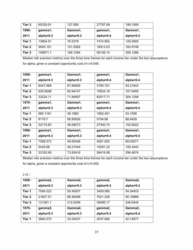
Tier 3 60329.91 127.695 27797.69 199.1595

1990-

2011

gamma1,

alpha=0.3

Gamma1,

alpha=0.3

gamma1,

alpha=0.4

Gamma1,

alpha=0.4

Tier 1 13904.51 76.5379 7474.852 125.0805

Tier 2 9545.191 101.5592 16913.03 183.9746

Tier 3 108871.1 169.1294 58126.14 359.1286

Median risk aversion metrics over the three time frames for each income tier under the two assumptions

for alpha, given a constant opportunity cost of rf=0.045.

1950-

2011

gamma1,

alpha=0.3

Gamma1,

alpha=0.3

gamma1,

alpha=0.4

Gamma1,

alpha=0.4

Tier 1 8447.668 87.89565 3790.751 93.21943

Tier 2 935.6598 60.94747 10634.16 107.9495

Tier 3 33224.11 71.84697 82517.71 304.1256

1970-

2011

gamma1,

alpha=0.3

Gamma1,

alpha=0.3

gamma1,

alpha=0.4

Gamma1,

alpha=0.4

Tier 1 960.1161 39.1983 1562.401 53.1508

Tier 2 8179.7 68.95626 5754.88 88.6428

Tier 3 32174.83 48.08273 27300.74 152.8522

1990-

2011

gamma1,

alpha=0.3

Gamma1,

alpha=0.3

gamma1,

alpha=0.4

Gamma1,

alpha=0.4

Tier 1 7289.072 48.65406 5081.822 99.02071

Tier 2 5429.68 49.27445 10291.23 150.3442

Tier 3 22183.95 73.93416 58419.08 296.4674

Median risk aversion metrics over the three time frames for each income tier under the two assumptions

for alpha, given a constant opportunity cost of rf=0.055.

L=2 ::

1950-

2011

gamma2,

alpha=0.3

Gamma2,

alpha=0.3

gamma2,

alpha=0.4

Gamma2,

alpha=0.4

Tier 1 7594.523 59.40007 3409.085 54.54403

Tier 2 21607.51 86.58498 7021.209 90.16888

Tier 3 131381.1 212.6399 39496.17 248.6444

1970-

2011

gamma2,

alpha=0.3

Gamma2,

alpha=0.3

gamma2,

alpha=0.4

Gamma2,

alpha=0.4

Tier 1 3800.572 33.24037 2037.682 42.14677

38

Tier 2 11775.08 66.37835 5650.186 69.33648

Tier 3 76834.16 116.108 20370.9 141.0344

1990-

2011

gamma2,

alpha=0.3

Gamma2,

alpha=0.3

gamma2,

alpha=0.4

Gamma2,

alpha=0.4

Tier 1 15073.94 72.40192 8857.499 108.3321

Tier 2 35884.51 112.0864 20330.45 118.9782

Tier 3 134313.7 214.7299 42597.52 234.6896

Median risk aversion metrics over the three time frames for each income tier under the two assumptions

for alpha, given a constant opportunity cost of rf=0.025.

1950-

2011

gamma2,

alpha=0.3

Gamma2,

alpha=0.3

gamma2,

alpha=0.4

Gamma2,

alpha=0.4

Tier 1 8388.3 54.11649 3964.199 52.40743

Tier 2 27580.44 62.69955 8221.303 79.83972

Tier 3 231890.1 158.2094 46180.83 221.3821

1970-

2011

gamma2,

alpha=0.3

Gamma2,

alpha=0.3

gamma2,

alpha=0.4

Gamma2,

alpha=0.4

Tier 1 2772.497 27.94699 1734.586 35.26029

Tier 2 15715.48 50.69245 6406.963 60.09672

Tier 3 50960.47 83.954 26405.76 119.445

1990-

2011

gamma2,

alpha=0.3

Gamma2,

alpha=0.3

gamma2,

alpha=0.4

Gamma2,

alpha=0.4

Tier 1 16422.76 54.44849 9236.037 74.35535

Tier 2 25222.28 81.18302 14216.59 102.4609

Tier 3 145602.1 158.2753 48457 206.4528

Median risk aversion metrics over the three time frames for each income tier under the two assumptions

for alpha, given a constant opportunity cost of rf=0.035.

1950-

2011

gamma2,

alpha=0.3

Gamma2,

alpha=0.3

gamma2,

alpha=0.4

Gamma2,

alpha=0.4

Tier 1 7206.076 48.78216 3577.149 49.25857

Tier 2 33758.57 42.31259 8752.897 65.70612

Tier 3 187336.1 102.2451 56795.8 186.4724

1970-

2011

gamma2,

alpha=0.3

Gamma2,

alpha=0.3

gamma2,

alpha=0.4

Gamma2,

alpha=0.4

Tier 1 2362.536 22.98957 1667.108 29.29132

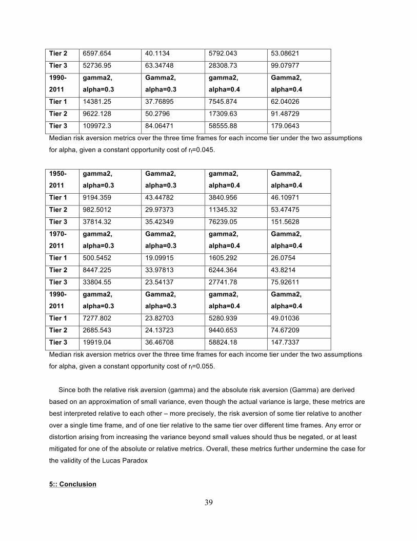
39

Tier 2 6597.654 40.1134 5792.043 53.08621

Tier 3 52736.95 63.34748 28308.73 99.07977

1990-

2011

gamma2,

alpha=0.3

Gamma2,

alpha=0.3

gamma2,

alpha=0.4

Gamma2,

alpha=0.4

Tier 1 14381.25 37.76895 7545.874 62.04026

Tier 2 9622.128 50.2796 17309.63 91.48729

Tier 3 109972.3 84.06471 58555.88 179.0643

Median risk aversion metrics over the three time frames for each income tier under the two assumptions

for alpha, given a constant opportunity cost of rf=0.045.

1950-

2011

gamma2,

alpha=0.3

Gamma2,

alpha=0.3

gamma2,

alpha=0.4

Gamma2,

alpha=0.4

Tier 1 9194.359 43.44782 3840.956 46.10971

Tier 2 982.5012 29.97373 11345.32 53.47475

Tier 3 37814.32 35.42349 76239.05 151.5628

1970-

2011

gamma2,

alpha=0.3

Gamma2,

alpha=0.3

gamma2,

alpha=0.4

Gamma2,

alpha=0.4

Tier 1 500.5452 19.09915 1605.292 26.0754

Tier 2 8447.225 33.97813 6244.364 43.8214

Tier 3 33804.55 23.54137 27741.78 75.92611

1990-

2011

gamma2,

alpha=0.3

Gamma2,

alpha=0.3

gamma2,

alpha=0.4

Gamma2,

alpha=0.4

Tier 1 7277.802 23.82703 5280.939 49.01036

Tier 2 2685.543 24.13723 9440.653 74.67209

Tier 3 19919.04 36.46708 58824.18 147.7337

Median risk aversion metrics over the three time frames for each income tier under the two assumptions

for alpha, given a constant opportunity cost of rf=0.055.

Since both the relative risk aversion (gamma) and the absolute risk aversion (Gamma) are derived

based on an approximation of small variance, even though the actual variance is large, these metrics are

best interpreted relative to each other – more precisely, the risk aversion of some tier relative to another

over a single time frame, and of one tier relative to the same tier over different time frames. Any error or

distortion arising from increasing the variance beyond small values should thus be negated, or at least

mitigated for one of the absolute or relative metrics. Overall, these metrics further undermine the case for

the validity of the Lucas Paradox

5:: Conclusion

40

The Lucas Paradox, predicated on the return on capital differential, appears to persist through time –

but at a much reduced level compared to what it once was. In other words, capital does flow from rich

countries to poor ones – but at an appropriately slow rate given how high the variance of returns in poor

countries is relative to rich ones. Here, “slow” reflects the finding that it took until the 1990-2011 period

before the geometric mean return of the poor countries converged to that of the middle income countries;

however, both the rich countries still generate the lowest geometric mean return, albeit with remarkably

much less variance (all of this evidence implicitly being at L=1). So, while there is evidence for some

convergence of returns, the convergence is far from complete and nuanced. The returns of poor countries

have converged down to the middle income countries but the variance of the middle income portfolio is

only around one sixth of the poor country portfolio. So, even if the poor countries have transitioned out of

high capital scarcity by achieving lower returns as of 2011, the representative investor should strongly

prefer middle income countries going forward, given the persistently high variance of returns in the poor

countries; the agent faces two groups of countries offering roughly the same reward, yet the poor group is

remarkably less stable. So, if it is acknowledged that the poor group has converged to the middle group,

the middle group must now converge with the rich group before the poor group can meaningfully

converge further. All of these considerations on convergence have been through the lens of L=1,

corresponding to a representative investor being credit-constrained when it comes to exploiting global

return imbalances. If it is acknowledged that the agent can borrow money in an attempt to arbitrage these

imbalances, then the estimation of the true degree of risk aversion is much more nuanced. Almost all of

the various risk aversion metrics, both relative and absolute under both assumptions for alpha over the

three time periods, did not steadily increase over time. However, the decreases came from the 1950 to

1970 period, in contrast to the apparent convergence in geometric mean return coming from the 1990 to

2011 period. Since the relative risk aversion is a nonlinear transformation of the mean/variance ratio and

the absolute metric is a linear one, if the variance shifts quickly down to the zero lower bound, then the

implied optimal leverage can increase rapidly, leaving the investor at L=1 and L=2 definitively under-

leveraged. However, if the investor is truly credit-constrained (L=1), then he might as well tolerate the

higher variance and not allocate to the rich countries.

Ultimately, unless interest rates are high (rf>>0.05), the representative investor might as well set L to 2

and invest in the middle income rich countries; allocating to the poor countries requires taking on much

more risk with little added diversification. In other words, the Lucas Paradox is highly overstated, now

more than ever.

41

6:: References

[1] Lucas jr., R. (1990). Why Doesn't Capital Flow from Rich to Poor Countries? The American Economic

Review, 80(2), 92-96. Retrieved on 2015-03-30: <http://www.jstor.org/stable/2006549>

[2] Henriksen, E., David, J., & Simonovska, I. (2014, December). The Risky Capital of Emerging Markets.

Retrieved on 2015-03-30: <http://www.nber.org/papers/w20769>

[3] Merton, R. (1969). Lifetime Portfolio Selection under Uncertainty: The Continuous-Time Case. The

Review of Economics and Statistics, 51(3), 247-257. Retrieved on 2015-03-30:

<http://www.jstor.org/stable/1926560>

[4] Sandmo, A. (1970). The Effect of Uncertainty on Saving Decisions. The Review of Economic

Studies, 37(3), 353-360. Retrieved on 2015-03-30: <http://www.jstor.org/stable/2296725>

[5] Kelly jr., J. (1956). A New Interpretation of Information Rate. The Bell System Technical Journal.

Retrieved on 2015-03-30: <http://www.princeton.edu/~wbialek/rome/refs/kelly_56.pdf>

[6] Jacquier, E., & Polson, N. (2011, August). Asset Allocation in Finance: A Bayesian Perspective.

Retrieved on 2015-03-30: <http://faculty.chicagobooth.edu/nicholas.polson/research/papers/Asset.pdf>

[7] Hidalgo, C., & Hausmann, R. (2009). The Building Blocks of Economic Complexity. Proceedings of the

National Academy of Sciences, 106(26), 10570-10575. Retrieved on 2015-03-30:

<http://www.ncbi.nlm.nih.gov/pmc/articles/PMC2705545/?tool=pmcentrez>

[8] Crucini, M., & Chen, K. (2014). Trends and Cycles in Small Open Economies: Making The Case For A

General Equilibrium Approach. CAMA Working paper 76/2014. Retrieved on 2015-03-30:

<http://dx.doi.org/10.2139/ssrn.2536634>

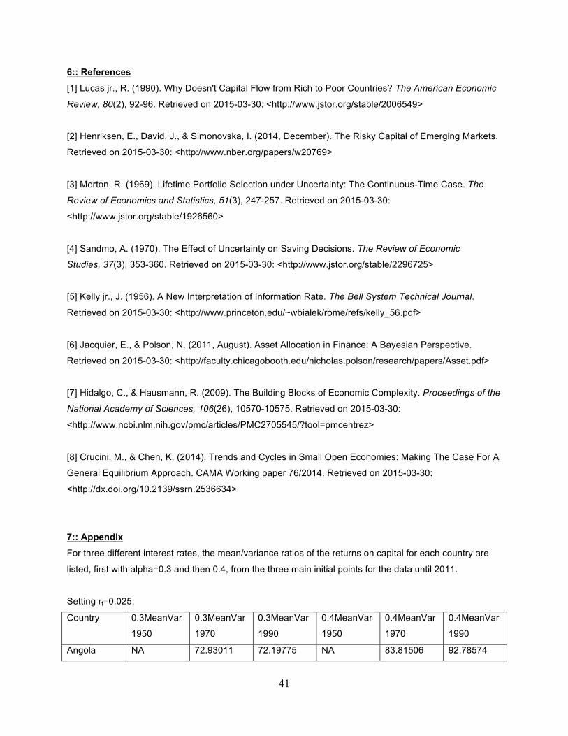
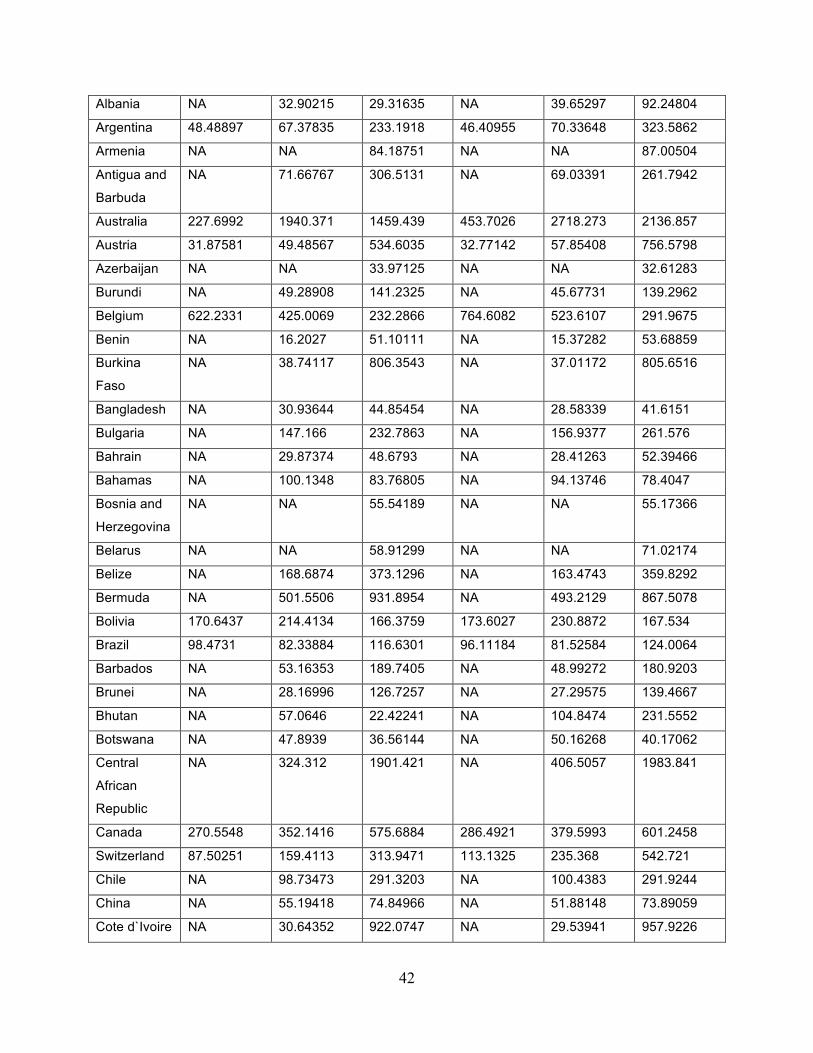
7:: Appendix

For three different interest rates, the mean/variance ratios of the returns on capital for each country are

listed, first with alpha=0.3 and then 0.4, from the three main initial points for the data until 2011.

Setting rf=0.025:

Country 0.3MeanVar

1950

0.3MeanVar

1970

0.3MeanVar

1990

0.4MeanVar

1950

0.4MeanVar

1970

0.4MeanVar

1990

Angola NA 72.93011 72.19775 NA 83.81506 92.78574

42

Albania NA 32.90215 29.31635 NA 39.65297 92.24804

Argentina 48.48897 67.37835 233.1918 46.40955 70.33648 323.5862

Armenia NA NA 84.18751 NA NA 87.00504

Antigua and

Barbuda

NA 71.66767 306.5131 NA 69.03391 261.7942

Australia 227.6992 1940.371 1459.439 453.7026 2718.273 2136.857

Austria 31.87581 49.48567 534.6035 32.77142 57.85408 756.5798

Azerbaijan NA NA 33.97125 NA NA 32.61283

Burundi NA 49.28908 141.2325 NA 45.67731 139.2962

Belgium 622.2331 425.0069 232.2866 764.6082 523.6107 291.9675

Benin NA 16.2027 51.10111 NA 15.37282 53.68859

Burkina

Faso

NA 38.74117 806.3543 NA 37.01172 805.6516

Bangladesh NA 30.93644 44.85454 NA 28.58339 41.6151

Bulgaria NA 147.166 232.7863 NA 156.9377 261.576

Bahrain NA 29.87374 48.6793 NA 28.41263 52.39466

Bahamas NA 100.1348 83.76805 NA 94.13746 78.4047

Bosnia and

Herzegovina

NA NA 55.54189 NA NA 55.17366

Belarus NA NA 58.91299 NA NA 71.02174

Belize NA 168.6874 373.1296 NA 163.4743 359.8292

Bermuda NA 501.5506 931.8954 NA 493.2129 867.5078

Bolivia 170.6437 214.4134 166.3759 173.6027 230.8872 167.534

Brazil 98.4731 82.33884 116.6301 96.11184 81.52584 124.0064

Barbados NA 53.16353 189.7405 NA 48.99272 180.9203

Brunei NA 28.16996 126.7257 NA 27.29575 139.4667

Bhutan NA 57.0646 22.42241 NA 104.8474 231.5552

Botswana NA 47.8939 36.56144 NA 50.16268 40.17062

Central

African

Republic

NA 324.312 1901.421 NA 406.5057 1983.841

Canada 270.5548 352.1416 575.6884 286.4921 379.5993 601.2458

Switzerland 87.50251 159.4113 313.9471 113.1325 235.368 542.721

Chile NA 98.73473 291.3203 NA 100.4383 291.9244

China NA 55.19418 74.84966 NA 51.88148 73.89059

Cote d`Ivoire NA 30.64352 922.0747 NA 29.53941 957.9226

43

Cameroon NA 45.25149 126.2539 NA 44.00651 125.8784

Congo,

Dem. Rep.

13.46321 13.46321 197.6771 12.44369 12.44369 237.4269

Congo,

Republic of

NA 14.08954 39.65875 NA 13.744 48.92471

Colombia 249.9317 281.1908 312.1161 269.9298 289.8198 313.3322

Comoros NA 145.6225 508.8505 NA 197.9849 1154.892

Cape Verde NA 2.877907 -133.196 NA 82.38268 464.6905

Costa Rica 120.9821 188.1355 362.9507 118.5138 181.9104 342.1929

Cyprus 88.88455 76.98374 451.086 149.2004 120.0207 557.8986

Czech

Republic

NA NA 242.8952 NA NA 310.6538

Germany 717.0934 801.4413 669.2859 874.0594 984.5024 779.5325

Djibouti NA 46.35142 127.9059 NA 44.60505 153.2558

Dominica NA 137.3354 401.1473 NA 134.8688 375.0134

Denmark 129.3431 305.277 267.8244 147.7629 384.8173 354.9405

Dominican

Republic

NA 65.01525 246.3 NA 59.8259 230.3873

Ecuador NA 90.53979 229.4159 NA 101.0158 295.0632

Egypt 13.31797 10.10638 29.09744 12.96513 9.882041 27.24355

Spain 60.72484 97.33079 124.1614 59.16656 101.4001 143.987

Estonia NA NA 131.7532 NA NA 138.9925

Ethiopia 22.71435 15.76227 18.74725 20.79051 14.4581 17.40638

Finland 82.80663 125.0419 104.1169 110.6749 217.5933 176.3376

Fiji NA 185.4792 143.1945 NA 183.3534 141.6513

France 194.1369 242.0406 165.6638 208.2195 267.3403 182.5914

Gabon NA 29.61894 30.7858 NA 31.13735 35.37364

United

Kingdom

389.8522 297.4556 197.5746 402.4312 309.9586 206.189

Georgia NA NA 14.94197 NA NA 15.91817

Ghana NA 127.2932 630.7172 NA 155.0847 727.4261

Guinea NA 223.869 169.2954 NA 210.2767 155.8176

Gambia, The NA 57.14003 78.80187 NA 56.08709 79.6408

Guinea-

Bissau

NA -69.0918 -338.195 NA 116.0912 243.253

Equatorial NA 19.80917 61.09712 NA 18.7554 57.51241

44

Guinea

Greece NA 203.4234 249.5951 NA 252.9781 317.1365

Grenada NA 29.71457 146.5999 NA 29.81305 154.0376

Guatemala 284.4767 274.6632 381.8698 273.1182 263.7042 359.6338

Hong Kong NA 34.97353 57.72041 NA 36.23143 72.28115

Honduras 97.38173 86.32635 63.68145 102.8056 93.17615 74.33271

Croatia NA NA 239.2758 NA NA 283.8525

Hungary NA 241.2137 197.353 NA 254.8568 208.0927

Indonesia NA 67.97495 36.56505 NA 60.76834 33.36653

India 287.4967 205.9544 169.1724 287.7167 218.3619 186.5325

Ireland 87.58498 73.64679 53.73917 88.16325 77.60535 54.84571

Iran NA 82.51945 918.7695 NA 93.87264 989.517

Iraq NA 53.38395 36.77336 NA 50.45028 35.71002

Iceland 253.0694 415.6427 342.2739 301.7866 514.291 436.9368

Israel 168.216 156.244 2706.193 182.2147 172.826 3278.063

Italy 110.671 123.0313 131.4768 133.6674 164.0482 229.3743

Jamaica NA 120.1949 612.8083 NA 119.4053 607.4725

Jordan NA 23.62776 45.25691 NA 22.91455 55.02381

Japan 48.17864 63.56022 86.76859 53.18724 80.70608 185.0654

Kazakhstan NA NA 40.40887 NA NA 47.81475

Kenya 114.7956 104.8858 185.0136 112.9213 104.2692 190.3839

Kyrgyzstan NA NA 53.2818 NA NA 51.23514

Cambodia NA 100.934 2564.38 NA 92.88001 2440.961

St. Kitts &

Nevis

NA 146.1474 175.9195 NA 142.0408 170.0494

Korea,

Republic of

NA 102.7613 88.34185 NA 107.6853 98.38969

Kuwait NA 32.84571 106.0482 NA 31.81037 109.3042

Laos NA 125.4702 136.846 NA 132.0003 139.5311

Lebanon NA 19.3385 56.28304 NA 22.99029 94.63017

Liberia NA 18.01557 3.104609 NA 21.16684 22.07918

St. Lucia NA 46.34921 111.5933 NA 44.62514 104.3378

Sri Lanka 33.23544 43.22205 120.5151 32.18858 44.13657 119.9782

Lesotho NA 21.63571 153.7642 NA 21.3021 201.9506

Lithuania NA NA 113.2345 NA NA 109.6726

Luxembourg 273.2702 292.1853 589.829 300.633 317.1666 649.7476

45

Latvia NA NA 123.2963 NA NA 133.1842

Macao NA 361.6297 215.1055 NA 351.8255 211.3988

Morocco 14.50232 12.1665 80.49774 13.87214 11.94366 117.5213

Moldova NA NA 30.71218 NA NA 45.44844

Madagascar NA 15.47694 25.04771 NA 15.02624 25.9641

Maldives NA 47.37609 80.03537 NA 45.63038 78.40671

Mexico 293.0045 248.1375 331.5124 276.7683 235.9252 327.6581

Macedonia NA NA 60.23694 NA NA 63.14134

Mali NA 33.06022 74.2691 NA 32.39877 76.9134

Malta NA 285.6961 225.788 NA 320.3941 254.2068

Montenegro NA NA 113.0864 NA NA 125.1107

Mongolia NA 26.22642 18.76981 NA 27.16023 24.60514

Mozambique NA 192.4652 591.5578 NA 178.6899 541.8755

Mauritania NA 90.6817 385.0873 NA 100.4746 566.9044

Mauritius 28.39755 22.31954 38.89386 27.37361 22.09398 43.89535

Malawi NA 41.88193 45.17937 NA 44.78389 65.75179

Malaysia NA 52.51596 140.4785 NA 90.31537 576.5563

Namibia NA 157.1165 687.3042 NA 166.5281 732.4259

Niger NA -2.4663 135.3136 NA 222.6899 512.3646

Nigeria 27.61294 35.42051 72.61932 26.00249 34.07287 66.36522

Netherlands 407.6908 448.0162 249.7372 439.1864 508.145 282.1985

Norway 124.3416 128.6366 187.4733 146.2168 166.3428 217.9383

Nepal NA 12.73087 59.1038 NA 11.73559 56.61137

New

Zealand

199.5806 235.1756 382.3024 212.7967 252.9968 400.3452

Oman NA 57.5326 59.70308 NA 60.9525 63.82349

Pakistan 104.162 73.07828 64.87921 98.74607 69.31783 62.70516

Panama 166.1649 217.4755 247.0768 159.2674 217.9239 249.1057

Peru 47.18601 39.86369 584.7862 45.27078 39.55859 741.8394

Philippines 68.74543 45.1976 124.424 64.59245 42.87443 129.9707

Poland NA 105.1232 237.7594 NA 107.1253 235.9577

Portugal 44.18734 51.933 192.3862 47.31232 61.12747 257.9728

Paraguay NA 28.00231 148.2764 NA 26.64438 143.6489

Qatar NA 39.09156 369.3544 NA 40.68243 421.2069

Romania NA 352.7971 499.4353 NA 389.549 550.6046

Russia NA NA 29.34558 NA NA 49.51534

46

Rwanda NA 11.14471 28.23826 NA 10.84542 26.97247

Saudi Arabia NA 24.44819 286.3916 NA 28.09259 461.734

Sudan NA 24.62353 14.39993 NA 24.5509 14.44106

Senegal NA 32.01526 39.65389 NA 32.05058 46.16646

Singapore NA 52.40314 82.05616 NA 59.67595 102.918

Sierra Leone NA 5.673694 4.762485 NA 5.447713 4.626135

El Salvador 68.64393 64.68585 165.9635 62.56793 58.71679 148.906

Serbia NA NA 87.14675 NA NA 128.5802

Sao Tome

and Principe

NA 35.67134 80.70799 NA 42.28704 161.2472

Suriname NA 36.74173 35.1257 NA 39.39092 47.78101

Slovak

Republic

NA NA 393.6406 NA NA 465.6976

Slovenia NA NA 216.3544 NA NA 266.1331

Sweden 126.1319 219.5235 210.4972 140.1223 248.3684 235.4216

Swaziland NA 13.50789 4.500217 NA 14.21483 9.017794

Syria NA 52.83489 30.64392 NA 50.54472 30.28632

Chad NA 166.8059 234.0824 NA 152.9863 217.9536

Togo NA 101.2978 820.2228 NA 106.9795 896.9012

Thailand 30.9827 20.97699 3.151309 34.70853 25.23885 42.46441

Tajikistan NA NA 23.32556 NA NA 28.23396

Turkmenista

n

NA NA 43.62851 NA NA 81.29808

Trinidad &

Tobago

35.35312 28.71391 232.0001 33.11724 27.29764 217.0915

Tunisia NA 19.7607 49.33316 NA 20.05091 69.94925

Turkey 132.7592 111.1847 183.96 141.7099 117.5722 189.7953

Taiwan NA 33.00931 68.89183 NA 32.22757 73.04834

Tanzania NA 27.36069 161.7034 NA 29.58642 207.2386

Uganda 52.15621 109.1329 185.3463 48.52013 98.19835 166.4189

Ukraine NA NA -14.5496 NA NA 43.63114

Uruguay 16.85419 50.46237 194.0906 16.14339 52.23876 222.666

United

States

575.6729 803.4952 943.5247 649.2681 883.5065 989.8239

Uzbekistan NA NA 163.7395 NA NA 150.8004

St.Vincent & NA 148.2701 114.4936 NA 137.8855 106.3751

47

Grenadines

Venezuela 84.0865 106.1145 205.94 91.16888 130.3364 267.4538

Vietnam NA 25.43629 14.26062 NA 23.07542 13.35594

Yemen NA NA 11.21805 NA NA 10.33135

South Africa 144.8349 260.8169 1872.698 153.3434 281.7735 2172.987

Zambia NA 18.10164 74.18451 NA 17.89676 86.28061

Zimbabwe NA 18.81833 18.17095 NA 19.0253 18.30986

Setting rf=0.035:

Country 0.3MeanVar

1950

0.3MeanVar

1970

0.3MeanVar

1990

0.4MeanVar

1950

0.4MeanVar

1970

0.4MeanVar

1990

Angola NA 51.35007 43.2652 NA 70.81717 75.3609

Albania NA 21.10347 -29.4205 NA 32.66119 56.62992

Argentina 41.0568 51.69245 128.003 42.05513 61.09672 256.3747

Armenia NA NA 68.98026 NA NA 77.54036

Antigua and

Barbuda

NA 67.55964 283.91 NA 66.33404 248.976

Australia 126.7708 1185.363 900.9908 369.9197 2240.159 1757.041

Austria 27.16751 36.12569 257.3196 29.85275 49.79977 599.3117

Azerbaijan NA NA 29.84948 NA NA 30.12418

Burundi NA 45.6212 124.5114 NA 43.3517 128.6038

Belgium 427.6763 288.9624 156.248 646.2634 441.7358 245.7671

Benin NA 15.33611 43.98197 NA 14.80302 49.14063

Burkina

Faso

NA 35.54261 694.5236 NA 34.97724 736.5887

Bangladesh NA 28.97107 40.05107 NA 27.34662 38.75422

Bulgaria NA 126.3443 188.7433 NA 143.5317 233.6511

Bahrain NA 26.58701 37.83672 NA 26.37999 45.74132

Bahamas NA 94.42702 78.37841 NA 90.46907 75.00847

Bosnia and

Herzegovina

NA NA 49.66146 NA NA 51.45767

Belarus NA NA 38.48195 NA NA 58.89211

Belize NA 162.7274 359.783 NA 159.3978 350.7674

Bermuda NA 479.8201 889.9656 NA 478.2939 840.3549

Bolivia 149.0792 190.155 148.6571 159.9941 214.429 156.1146

Brazil 84.95648 69.80771 90.53362 87.85315 73.88968 108.2468

48

Barbados NA 51.21062 183.9559 NA 47.71151 176.9639

Brunei NA 25.26733 100.8454 NA 25.46774 123.1514

Bhutan NA 9.779249 -168.624 NA 76.33252 128.3923

Botswana NA 41.85856 30.65215 NA 46.36628 36.57836

Central

African

Republic

NA 223.7062 1403.302 NA 341.1307 1697.318

Canada 222.3388 279.0759 445.7283 256.5394 335.1038 526.4777

Switzerland 62.30228 86.97386 121.3888 96.98223 191.5736 425.9859

Chile NA 86.51823 246.4314 NA 92.67031 264.9928

China NA 49.77523 63.30951 NA 48.51307 66.85582

Cote d`Ivoire NA 28.92292 838.2114 NA 28.40265 901.4429

Cameroon NA 41.78597 112.9855 NA 41.77447 117.5108

Congo,

Dem. Rep.

12.0689 12.0689 100.5999 11.58414 11.58414 181.8164

Congo,

Republic of

NA 13.18497 31.18055 NA 13.15151 43.3971

Colombia 188.201 219.5126 232.5547 234.3905 254.8511 270.9994

Comoros NA 47.06811 -184.256 NA 148.2242 753.2989

Cape Verde NA -59.3908 -602.156 NA 42.84284 207.1635

Costa Rica 113.5883 174.8195 334.3738 113.6022 173.3523 324.5364

Cyprus 16.8185 21.91538 267.9119 106.4314 87.58107 448.8912

Czech

Republic

NA NA 160.2388 NA NA 259.1221

Germany 479.0918 517.4836 449.4536 731.442 816.6856 652.5655

Djibouti NA 39.10642 84.66858 NA 40.31715 126.6422

Dominica NA 134.6138 391.8751 NA 132.9289 368.759

Denmark 97.65679 200.6171 162.3547 128.2325 321.0284 291.1383

Dominican

Republic

NA 59.23931 213.8037 NA 56.29986 211.1685

Ecuador NA 68.86376 131.5849 NA 87.88208 239.0858

Egypt 13.06872 9.874948 27.56198 12.78939 9.719806 26.26397

Spain 50.80781 73.63112 84.63709 53.41553 87.96331 120.6748

Estonia NA NA 110.4526 NA NA 125.6424

Ethiopia 21.94497 15.20391 17.41801 20.28628 14.09212 16.56483

Finland 48.34563 34.7312 32.19544 89.64389 162.0825 132.0486

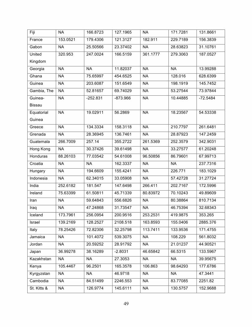
49

Fiji NA 166.8723 127.1965 NA 171.7281 131.8661

France 153.0521 179.4306 121.3127 182.911 229.7189 156.3839

Gabon NA 25.50566 23.37402 NA 28.63823 31.10761

United

Kingdom

320.953 247.0024 166.5159 361.1777 279.3063 187.0527

Georgia NA NA 11.82037 NA NA 13.99288

Ghana NA 75.65997 454.6525 NA 128.016 628.6399

Guinea NA 203.6087 151.6549 NA 198.1919 145.7452

Gambia, The NA 52.81657 69.74029 NA 53.27544 73.97844

Guinea-

Bissau

NA -252.831 -873.966 NA 10.44885 -72.5484

Equatorial

Guinea

NA 19.02911 56.2869 NA 18.23567 54.53338

Greece NA 134.3334 158.3118 NA 210.7797 261.6481

Grenada NA 28.36945 136.7461 NA 28.87923 147.2459

Guatemala 266.7009 257.14 355.2722 261.5369 252.3579 342.9031

Hong Kong NA 30.37426 39.61498 NA 33.27577 61.20248

Honduras 88.26103 77.03542 54.61008 96.50856 86.79601 67.99713

Croatia NA NA 162.3337 NA NA 237.7316

Hungary NA 194.6609 155.4241 NA 226.771 183.1029

Indonesia NA 62.34015 33.05908 NA 57.42728 31.27724

India 252.6182 181.547 147.6498 266.411 202.7167 172.5996

Ireland 75.63399 61.50811 45.71339 80.83972 70.10243 49.89609

Iran NA 59.64843 556.6826 NA 80.38864 810.7134

Iraq NA 47.24868 31.73547 NA 46.75394 32.68343

Iceland 173.7961 256.0954 200.9516 253.2531 419.9875 353.265

Israel 139.2169 128.2527 2108.518 163.8593 155.0406 2885.376

Italy 78.25426 72.82306 32.25798 113.7411 133.9536 171.4755

Jamaica NA 101.4072 539.3075 NA 108.229 561.8032

Jordan NA 20.59252 28.91792 NA 21.01237 44.90521

Japan 36.99278 38.16289 -2.8031 46.65842 66.5315 133.5967

Kazakhstan NA NA 27.3053 NA NA 39.95675

Kenya 105.4467 96.2501 165.3578 106.863 98.64293 177.6786

Kyrgyzstan NA NA 46.9718 NA NA 47.3441

Cambodia NA 84.51499 2246.553 NA 83.77085 2251.82

St. Kitts & NA 126.9774 145.6111 NA 130.5757 152.9688

50

Nevis

Korea,

Republic of

NA 84.15304 65.45134 NA 96.56366 85.24334

Kuwait NA 28.40468 82.88042 NA 29.08668 95.43101

Laos NA 102.9602 108.5134 NA 118.1312 123.4615

Lebanon NA 13.85032 6.658947 NA 19.62127 68.74999

Liberia NA 13.89205 -10.3495 NA 18.70899 14.83603

St. Lucia NA 45.02123 107.799 NA 43.70864 101.8187

Sri Lanka 30.33012 37.60455 101.0246 30.3337 40.58497 108.5069

Lesotho NA 17.79404 67.25935 NA 18.98984 151.4505

Lithuania NA NA 100.5097 NA NA 101.7564

Luxembourg 211.8734 218.9547 445.8773 263.5863 274.9381 565.5967

Latvia NA NA 96.69801 NA NA 117.0361

Macao NA 314.3597 185.9184 NA 322.7411 193.4294

Morocco 13.61845 11.18538 48.76609 13.29655 11.31016 97.39036

Moldova NA NA 9.929153 NA NA 33.54799

Madagascar NA 14.54116 22.04668 NA 14.40507 24.04275

Maldives NA 43.35912 69.17084 NA 43.09015 71.93704

Mexico 257.6309 217.0767 282.2785 255.6632 217.3648 297.8155

Macedonia NA NA 48.53704 NA NA 56.06843

Mali NA 31.70119 69.39398 NA 31.47133 73.56881

Malta NA 224.115 171.7479 NA 280.7809 220.8843

Montenegro NA NA 82.18302 NA NA 106.7139

Mongolia NA 21.82478 11.34898 NA 24.45263 20.12171

Mozambique NA 176.2605 534.5823 NA 168.5858 507.3473

Mauritania NA 67.466 259.48 NA 86.287 472.1486

Mauritius 26.7358 20.6805 31.94473 26.27075 21.00583 39.48027

Malawi NA 33.82985 22.84716 NA 40.00687 52.8337

Malaysia NA 28.36676 -99.6458 NA 73.5774 409.5949

Namibia NA 129.8482 552.7148 NA 149.8752 652.1111

Niger NA -172.458 -169.405 NA 109.0509 308.2717

Nigeria 25.8831 32.23643 65.10117 24.8845 32.05581 61.97849

Netherlands 305.1619 323.4865 180.9681 380.3887 434.545 241.6192

Norway 89.48308 81.82333 133.5527 124.8246 137.4058 185.1946

Nepal NA 11.98109 48.73274 NA 11.25439 50.52366

New 165.3666 188.0367 315.6785 191.511 224.5921 360.0064

51

Zealand

Oman NA 50.83952 49.73146 NA 56.66169 57.96921

Pakistan 96.13873 67.03055 57.69372 93.66836 65.53553 58.32692

Panama 151.45 198.0661 225.02 150.0999 205.3881 234.8206

Peru 41.20431 33.19698 341.4202 41.67481 35.63002 599.0487

Philippines 60.2104 39.3556 93.82669 59.68089 39.50008 112.9837

Poland NA 85.75496 185.5712 NA 95.58944 206.8676

Portugal 37.03425 38.7437 101.9586 42.8088 53.08237 208.038

Paraguay NA 25.52657 121.8135 NA 25.11292 128.8487

Qatar NA 34.18015 293.6484 NA 37.52215 373.7083

Romania NA 265.8492 369.7526 NA 337.0684 473.6171

Russia NA NA 6.60997 NA NA 35.93073

Rwanda NA 10.93971 27.04522 NA 10.70043 26.17615

Saudi Arabia NA 17.73052 78.19863 NA 23.99704 341.4836

Sudan NA 24.28795 14.16829 NA 24.30515 14.27115

Senegal NA 27.73141 28.88245 NA 29.35933 39.53382

Singapore NA 43.0574 58.20864 NA 53.62326 88.39966

Sierra Leone NA 5.588336 4.507455 NA 5.38759 4.454592

El Salvador 65.33468 61.11278 154.4678 60.4748 56.49268 141.9053

Serbia NA NA 33.55132 NA NA 97.03572

Sao Tome

and Principe

NA 28.49703 29.85561 NA 37.54334 126.3482

Suriname NA 30.60554 23.62647 NA 35.46534 40.10166

Slovak

Republic

NA NA 277.5865 NA NA 396.5784

Slovenia NA NA 151.5218 NA NA 225.9128

Sweden 104.8028 171.6276 166.8222 126.4697 219.3075 208.8864

Swaziland NA 11.8247 1.30519 NA 13.16203 7.149903

Syria NA 48.4689 27.44209 NA 47.79979 28.2839

Chad NA 160.1215 225.2227 NA 148.6254 212.0741

Togo NA 82.2743 648.7544 NA 95.17111 788.9818

Thailand 26.18911 16.50478 -20.6077 31.54593 22.37306 27.93781

Tajikistan NA NA 13.87373 NA NA 22.71486

Turkmenista

n

NA NA 2.166084 NA NA 56.93229

Trinidad & 33.83316 27.28688 214.6768 32.13225 26.37019 206.4339

52

Tobago

Tunisia NA 17.69372 30.37936 NA 18.72603 58.29834

Turkey 114.3226 93.84142 160.4566 129.8746 106.9364 175.1946

Taiwan NA 30.22284 58.72434 NA 30.47714 66.74665

Tanzania NA 23.19698 116.1339 NA 26.94257 178.6829

Uganda 50.02257 103.4811 174.5821 47.13397 94.70793 159.7868

Ukraine NA NA -64.6643 NA NA 15.00434

Uruguay 15.27076 41.24807 143.0145 15.15221 46.62435 191.029

United

States

456.1062 618.1208 725.1521 572.9429 771.7229 864.92

Uzbekistan NA NA 152.5038 NA NA 143.7241

St.Vincent &

Grenadines

NA 142.8782 110.0714 NA 134.3158 103.4609

Venezuela 63.69955 68.76731 118.8078 78.9375 107.6081 215.0833

Vietnam NA 24.16347 13.25092 NA 22.26171 12.70575

Yemen NA NA 10.84511 NA NA 10.08543

South Africa 128.0071 223.9281 1577.246 142.2417 257.9835 1973.682

Zambia NA 16.40193 56.68037 NA 16.7987 75.3498

Zimbabwe NA 18.54193 17.96076 NA 18.82007 18.15372

Setting rf=0.045

Country 0.3MeanVar

1950

0.3MeanVar

1970

0.3MeanVar

1990

0.4MeanVar

1950

0.4MeanVar

1970

0.4MeanVar

1990

Angola NA 29.77003 14.33265 NA 57.81928 57.93605

Albania NA 9.304802 -88.1573 NA 25.66941 21.01181

Argentina 33.62463 36.00655 22.81408 37.70071 51.85697 189.1632

Armenia NA NA 53.773 NA NA 68.07568

Antigua and

Barbuda

NA 63.45161 261.3069 NA 63.63417 236.1577

Australia 25.84234 430.3552 342.5427 286.1368 1762.045 1377.225

Austria 22.45921 22.76571 -19.9644 26.93408 41.74545 442.0436

Azerbaijan NA NA 25.72772 NA NA 27.63553

Burundi NA 41.95332 107.7903 NA 41.02609 117.9114

Belgium 233.1195 152.918 80.20946 527.9186 359.8609 199.5666

Benin NA 14.46952 36.86283 NA 14.23322 44.59268

Burkina NA 32.34406 582.6929 NA 32.94276 667.5257

53

Faso

Bangladesh NA 27.00569 35.24761 NA 26.10984 35.89334

Bulgaria NA 105.5227 144.7004 NA 130.1257 205.7262

Bahrain NA 23.30027 26.99415 NA 24.34734 39.08798

Bahamas NA 88.71923 72.98877 NA 86.80067 71.61223

Bosnia and

Herzegovina

NA NA 43.78102 NA NA 47.74168

Belarus NA NA 18.05092 NA NA 46.76249

Belize NA 156.7673 346.4364 NA 155.3213 341.7057

Bermuda NA 458.0896 848.0358 NA 463.375 813.202

Bolivia 127.5146 165.8966 130.9382 146.3855 197.9708 144.6951

Brazil 71.43985 57.27658 64.43718 79.59446 66.25352 92.48729

Barbados NA 49.25772 178.1714 NA 46.4303 173.0075

Brunei NA 22.3647 74.9651 NA 23.63974 106.836

Bhutan NA -37.5061 -359.67 NA 47.81769 25.22937

Botswana NA 35.82322 24.74286 NA 42.56987 32.9861

Central

African

Republic

NA 123.1003 905.1824 NA 275.7557 1410.796

Canada 174.1228 206.0102 315.7682 226.5868 290.6084 451.7097

Switzerland 37.10204 14.53645 -71.1695 80.83197 147.7791 309.2507

Chile NA 74.30174 201.5425 NA 84.90237 238.0612

China NA 44.35627 51.76935 NA 45.14465 59.82105

Cote d`Ivoire NA 27.20231 754.3481 NA 27.26588 844.9631

Cameroon NA 38.32045 99.7171 NA 39.54242 109.1432

Congo,

Dem. Rep.

10.67459 10.67459 3.522743 10.7246 10.7246 126.2059

Congo,

Republic of

NA 12.2804 22.70234 NA 12.55901 37.86949

Colombia 126.4702 157.8345 152.9932 198.8513 219.8825 228.6665

Comoros NA -51.4863 -877.363 NA 98.4636 351.7057

Cape Verde NA -121.66 -1071.12 NA 3.302996 -50.3635

Costa Rica 106.1945 161.5036 305.797 108.6906 164.7942 306.8799

Cyprus -55.2476 -33.153 84.7378 63.66251 55.14148 339.8838

Czech

Republic

NA NA 77.58241 NA NA 207.5903

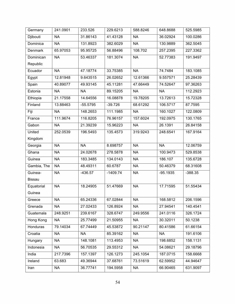
54

Germany 241.0901 233.526 229.6213 588.8246 648.8688 525.5985

Djibouti NA 31.86143 41.43128 NA 36.02924 100.0286

Dominica NA 131.8923 382.6029 NA 130.9889 362.5045

Denmark 65.97053 95.95725 56.88496 108.702 257.2395 227.3362

Dominican

Republic

NA 53.46337 181.3074 NA 52.77383 191.9497

Ecuador NA 47.18774 33.75385 NA 74.7484 183.1085

Egypt 12.81948 9.643515 26.02652 12.61366 9.557571 25.28439

Spain 40.89077 49.93145 45.11281 47.66449 74.52647 97.36263

Estonia NA NA 89.15205 NA NA 112.2923

Ethiopia 21.17558 14.64556 16.08878 19.78205 13.72613 15.72328

Finland 13.88463 -55.5795 -39.726 68.61292 106.5717 87.7595

Fiji NA 148.2653 111.1985 NA 160.1027 122.0809

France 111.9674 116.8205 76.96157 157.6024 192.0975 130.1765

Gabon NA 21.39239 15.96223 NA 26.1391 26.84158

United

Kingdom

252.0539 196.5493 135.4573 319.9243 248.6541 167.9164

Georgia NA NA 8.698757 NA NA 12.06759

Ghana NA 24.02678 278.5878 NA 100.9473 529.8538

Guinea NA 183.3485 134.0143 NA 186.107 135.6728

Gambia, The NA 48.49311 60.6787 NA 50.46379 68.31608

Guinea-

Bissau

NA -436.57 -1409.74 NA -95.1935 -388.35

Equatorial

Guinea

NA 18.24905 51.47669 NA 17.71595 51.55434

Greece NA 65.24336 67.02844 NA 168.5812 206.1596

Grenada NA 27.02433 126.8924 NA 27.94541 140.4541

Guatemala 248.9251 239.6167 328.6747 249.9556 241.0116 326.1724

Hong Kong NA 25.77499 21.50955 NA 30.32011 50.1238

Honduras 79.14034 67.74449 45.53872 90.21147 80.41586 61.66154

Croatia NA NA 85.39162 NA NA 191.6106

Hungary NA 148.1081 113.4953 NA 198.6852 158.1131

Indonesia NA 56.70535 29.55312 NA 54.08621 29.18796

India 217.7396 157.1397 126.1273 245.1054 187.0715 158.6668

Ireland 63.683 49.36944 37.68761 73.51619 62.59952 44.94647

Iran NA 36.77741 194.5958 NA 66.90465 631.9097

55

Iraq NA 41.1134 26.69758 NA 43.0576 29.65684

Iceland 94.52283 96.5481 59.62936 204.7196 325.684 269.5932

Israel 110.2178 100.2614 1510.843 145.5039 137.2552 2492.689

Italy 45.83758 22.61484 -66.9609 93.81473 103.859 113.5767

Jamaica NA 82.61942 465.8067 NA 97.0527 516.134

Jordan NA 17.55728 12.57892 NA 19.11019 34.7866

Japan 25.80693 12.76556 -92.3748 40.1296 52.35691 82.12813

Kazakhstan NA NA 14.20173 NA NA 32.09874

Kenya 96.09774 87.61443 145.7019 100.8048 93.01664 164.9732

Kyrgyzstan NA NA 40.66181 NA NA 43.45305

Cambodia NA 68.09599 1928.726 NA 74.66169 2062.678

St. Kitts &

Nevis

NA 107.8074 115.3027 NA 119.1106 135.8882

Korea,

Republic of

NA 65.5448 42.56082 NA 85.442 72.09698

Kuwait NA 23.96365 59.7126 NA 26.36298 81.55786

Laos NA 80.45025 80.18072 NA 104.2621 107.3919

Lebanon NA 8.36213 -42.9651 NA 16.25225 42.86981

Liberia NA 9.76853 -23.8037 NA 16.25113 7.592867

St. Lucia NA 43.69326 104.0048 NA 42.79215 99.29968

Sri Lanka 27.4248 31.98704 81.53415 28.47881 37.03337 97.03552

Lesotho NA 13.95236 -19.2455 NA 16.67757 100.9504

Lithuania NA NA 87.7849 NA NA 93.8401

Luxembourg 150.4765 145.7241 301.9257 226.5397 232.7095 481.4458

Latvia NA NA 70.0997 NA NA 100.888

Macao NA 267.0897 156.7312 NA 293.6566 175.4599

Morocco 12.73458 10.20426 17.03444 12.72096 10.67665 77.25946

Moldova NA NA -10.8539 NA NA 21.64753

Madagascar NA 13.60538 19.04564 NA 13.7839 22.12141

Maldives NA 39.34215 58.30632 NA 40.54991 65.46737

Mexico 222.2574 186.0159 233.0447 234.5581 198.8044 267.9729

Macedonia NA NA 36.83713 NA NA 48.99552

Mali NA 30.34216 64.51887 NA 30.54388 70.22421

Malta NA 162.5339 117.7079 NA 241.1677 187.5619

Montenegro NA NA 51.2796 NA NA 88.31718

Mongolia NA 17.42314 3.928146 NA 21.74503 15.63828

56

Mozambique NA 160.0557 477.6069 NA 158.4816 472.819

Mauritania NA 44.2503 133.8726 NA 72.09943 377.3927

Mauritius 25.07404 19.04146 24.99561 25.1679 19.91769 35.0652

Malawi NA 25.77776 0.514956 NA 35.22984 39.91561

Malaysia NA 4.217555 -339.77 NA 56.83942 242.6335

Namibia NA 102.5799 418.1254 NA 133.2224 571.7963

Niger NA -342.449 -474.124 NA -4.5881 104.1789

Nigeria 24.15325 29.05234 57.58302 23.76652 30.03875 57.59176

Netherlands 202.6329 198.9569 112.199 321.5911 360.9449 201.0399

Norway 54.62458 35.01003 79.63209 103.4325 108.4689 152.451

Nepal NA 11.23131 38.36168 NA 10.7732 44.43594

New

Zealand

131.1527 140.8977 249.0546 170.2252 196.1873 319.6675

Oman NA 44.14643 39.75984 NA 52.37087 52.11492

Pakistan 88.11549 60.98281 50.50823 88.59065 61.75322 53.94868

Panama 136.7351 178.6568 202.9632 140.9324 192.8523 220.5354

Peru 35.2226 26.53026 98.05407 38.07883 31.70146 456.2579

Philippines 51.67537 33.51361 63.2294 54.76933 36.12573 95.99673

Poland NA 66.38675 133.383 NA 84.05357 177.7774

Portugal 29.88116 25.5544 11.53098 38.30527 45.03726 158.1032

Paraguay NA 23.05084 95.35066 NA 23.58145 114.0485

Qatar NA 29.26874 217.9423 NA 34.36186 326.2098

Romania NA 178.9013 240.07 NA 284.5878 396.6295

Russia NA NA -16.1256 NA NA 22.34611

Rwanda NA 10.7347 25.85218 NA 10.55544 25.37983

Saudi Arabia NA 11.01284 -129.994 NA 19.90148 221.2332

Sudan NA 23.95237 13.93666 NA 24.05941 14.10125

Senegal NA 23.44755 18.111 NA 26.66808 32.90117

Singapore NA 33.71165 34.36113 NA 47.57057 73.88127

Sierra Leone NA 5.502978 4.252424 NA 5.327468 4.283048

El Salvador 62.02543 57.5397 142.972 58.38168 54.26857 134.9046

Serbia NA NA -20.0441 NA NA 65.49125

Sao Tome

and Principe

NA 21.32272 -20.9968 NA 32.79965 91.44912

Suriname NA 24.46936 12.12724 NA 31.53975 32.42231

Slovak NA NA 161.5324 NA NA 327.4592

57

Republic

Slovenia NA NA 86.68929 NA NA 185.6924

Sweden 83.47358 123.7317 123.1472 112.8171 190.2466 182.3512

Swaziland NA 10.14151 -1.88984 NA 12.10922 5.282011

Syria NA 44.10291 24.24027 NA 45.05486 26.28148

Chad NA 153.437 216.3631 NA 144.2645 206.1946

Togo NA 63.25076 477.286 NA 83.36268 681.0624

Thailand 21.39553 12.03256 -44.3667 28.38333 19.50727 13.41121

Tajikistan NA NA 4.421906 NA NA 17.19576

Turkmenista

n

NA NA -39.2963 NA NA 32.5665

Trinidad &

Tobago

32.31319 25.85985 197.3534 31.14727 25.44274 195.7764

Tunisia NA 15.62675 11.42556 NA 17.40116 46.64743

Turkey 95.88603 76.49811 136.9532 118.0392 96.30054 160.5939

Taiwan NA 27.43638 48.55685 NA 28.7267 60.44495

Tanzania NA 19.03326 70.56443 NA 24.29872 150.1272

Uganda 47.88894 97.82929 163.8179 45.74782 91.21751 153.1547

Ukraine NA NA -114.779 NA NA -13.6224

Uruguay 13.68732 32.03378 91.93843 14.16103 41.00994 159.392

United

States

336.5394 432.7465 506.7795 496.6176 659.9393 740.0161

Uzbekistan NA NA 141.268 NA NA 136.6478

St.Vincent &

Grenadines

NA 137.4863 105.6493 NA 130.7461 100.5467

Venezuela 43.31259 31.42013 31.67555 66.70612 84.87969 162.7127

Vietnam NA 22.89065 12.24122 NA 21.44799 12.05556

Yemen NA NA 10.47217 NA NA 9.839506

South Africa 111.1793 187.0394 1281.793 131.14 234.1936 1774.378

Zambia NA 14.70222 39.17623 NA 15.70063 64.41899

Zimbabwe NA 18.26553 17.75056 NA 18.61484 17.99757

58

59

######################################

# R Appendix

## curve of one plus geometric mean against leverage

## for the empirical distribution of all return observations given alpha=0.3

r=0.05

g=NULL

for(k in seq(9,-(1+r)/(exp(min(na.omit(alpha0.3returns)))-1-r),0.001))

{

rescaled_returns=k*exp(na.omit(alpha0.3returns))-(k-1)-r*(k-1)-1

y=exp(mean(log(1+rescaled_returns)))

g=rbind(g,c(k,y))

}