the lsst dark energy science collaboration (desc) science
TRANSCRIPT

Rubin Observatory
LSST DESCScience Requirements Document
Version 1.0.2Date: Wednesday 8th September, 2021
arX
iv:1
809.
0166
9v2
[as
tro-
ph.C
O]
6 S
ep 2
021
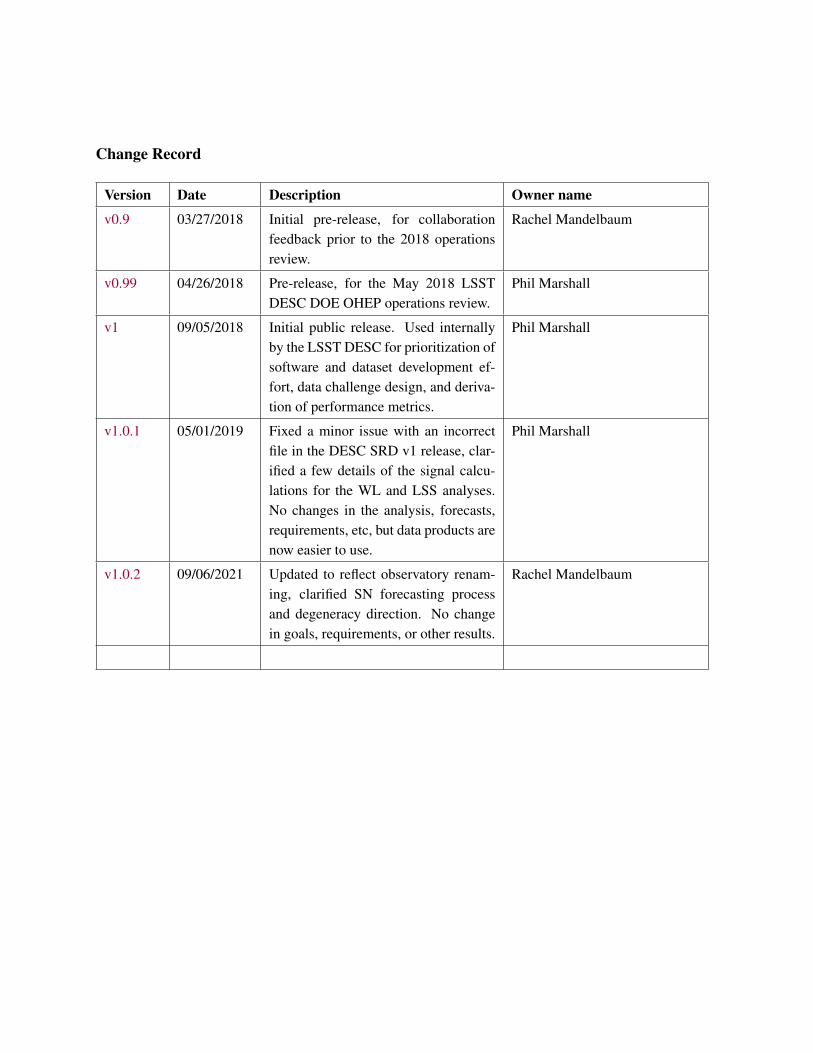
Change Record
Version Date Description Owner name
v0.9 03/27/2018 Initial pre-release, for collaborationfeedback prior to the 2018 operationsreview.
Rachel Mandelbaum
v0.99 04/26/2018 Pre-release, for the May 2018 LSSTDESC DOE OHEP operations review.
Phil Marshall
v1 09/05/2018 Initial public release. Used internallyby the LSST DESC for prioritization ofsoftware and dataset development ef-fort, data challenge design, and deriva-tion of performance metrics.
Phil Marshall
v1.0.1 05/01/2019 Fixed a minor issue with an incorrectfile in the DESC SRD v1 release, clar-ified a few details of the signal calcu-lations for the WL and LSS analyses.No changes in the analysis, forecasts,requirements, etc, but data products arenow easier to use.
Phil Marshall
v1.0.2 09/06/2021 Updated to reflect observatory renam-ing, clarified SN forecasting processand degeneracy direction. No changein goals, requirements, or other results.
Rachel Mandelbaum

ContributorsContributors to the DESC SRD effort are listed in the table below, with leading contributions shown inbold and affiliations indicated in the notes below the table.
Name ContributionDavid Alonso1,2 Forecasting guidance, LSS analysis definition, WL forecast cross-checkHumna Awan3 Input on survey definition based on OpSim v3 minion_1016Rahul Biswas4 SN analysis definition, systematics treatmentJonathan Blazek5,6 Forecasting guidance, review of complete draftPatricia Burchat7,8 Initial organization, WL systematic uncertainties listElisa Chisari2 Forecasting guidance, review of complete draftTom Collett9 SL forecaster, SL analysis definitionIan Dell’Antonio10 CL analysis definitionSeth Digel8,11 Review of complete draftTim Eifler12,13 Lead forecaster, WL+LSS+CL analysis and systematics definition,
joint probe covariance computationJosh Frieman14,15 Review of complete draftEric Gawiser3 Project management, scientific guidance, text editingDaniel Goldstein16,17,18 SL analysis definitionRenée Hložek19,20 SN forecaster, SN analysis definition, systematics treatmentIsobel Hook21 Consultation on 4MOST capabilities for SN science caseŽeljko Ivezic22 Review of complete draft, feedback on connection to LSST SRDSteven Kahn7,8,11,23 Review of document and feedback on connection to LSST SRDSowmya Kamath7,8 WL systematic uncertainties listDavid Kirkby24 Initial organization, source sample characterization, review of draftTom Kitching25 WL analysis definitionElisabeth Krause12 Forecasting guidance, Fisher software, CosmoLike infrastructurePierre-François Leget7,8 WL systematic uncertainties listRachel Mandelbaum26 Lead author, scientific oversight, project managementPhil Marshall8,11 Initial organizational work, scientific guidance, text editingJosh Meyers7,8 WL systematic uncertainties listHironao Miyatake13,27,28 Cluster mass-observable relation software, CL forecasting guidanceJeff Newman29 Input on WL, LSS, and SN sample definition, review of complete draftBob Nichol9 Consultation on 4MOST capabilities for SN science caseEli Rykoff8,11 WL, LSS, and CL area definition including dust, depth constraintsF. Javier Sanchez24 WL source sample characterizationDaniel Scolnic15 SN analysis definition and forecastingAnže Slosar30 LSS analysis definitionMark Sullivan31 Consultation on 4MOST capabilities for SN science caseMichael Troxel6,32 Review of complete draft

1 School of Physics and Astronomy, Cardiff University2 Department of Physics, University of Oxford3 Department of Physics and Astronomy, Rutgers University4 Oskar Klein Centre, Department of Physics, Stockholm University5 SNSF Ambizione, Laboratory of Astrophysics, École Polytechnique Fédérale de Lausanne (EPFL)6 Center for Cosmology and Astroparticle Physics, Ohio State University7 Department of Physics, Stanford University8 Kavli Institute for Particle Astrophysics and Cosmology (KIPAC), Stanford University9 Institute of Cosmology and Gravitation, University of Portsmouth10 Department of Physics, Brown University11 SLAC National Accelerator Laboratory12 Steward Observatory/Department of Astronomy, University of Arizona13 Jet Propulsion Laboratory, California Institute of Technology14 Fermi National Accelerator Laboratory15 Kavli Institute for Cosmological Physics, University of Chicago16 California Institute of Technology17 Lawrence Berkeley National Laboratory18 Department of Astronomy, University of California, Berkeley19 Department of Astronomy and Astrophysics, University of Toronto20 Dunlap Institute for Astronomy and Astrophysics, University of Toronto21 Department of Physics, Lancaster University22 Department of Astronomy, University of Washington23 Rubin Observatory Project24 Department of Physics and Astronomy, University of California, Irvine25 Mullard Space Science Laboratory, University College London26 McWilliams Center for Cosmology, Department of Physics, Carnegie Mellon University27 Nagoya University28 Kavli Institute for the Physics and Mathematics of the Universe (Kavli IPMU, WPI)29 Department of Physics and Astronomy and PITT PACC, University of Pittsburgh30 Physics Department, Brookhaven National Laboratory31 Department of Physics and Astronomy, University of Southampton32 Department of Physics, The Ohio State University

Contents
Contributors . . . . . . . . . . . . . . . . . . . . . . . . . . . . . . . . . . . . . . . . . . .Executive Summary and User Guide . . . . . . . . . . . . . . . . . . . . . . . . . . . . . . 11 Introduction . . . . . . . . . . . . . . . . . . . . . . . . . . . . . . . . . . . . . . . . 42 Definitions . . . . . . . . . . . . . . . . . . . . . . . . . . . . . . . . . . . . . . . . . 53 Objectives . . . . . . . . . . . . . . . . . . . . . . . . . . . . . . . . . . . . . . . . . 94 High-level requirements . . . . . . . . . . . . . . . . . . . . . . . . . . . . . . . . . . 105 Detailed requirements . . . . . . . . . . . . . . . . . . . . . . . . . . . . . . . . . . . 13
5.1 Large-scale structure . . . . . . . . . . . . . . . . . . . . . . . . . . . . . . . 165.2 Weak lensing (3×2-point) . . . . . . . . . . . . . . . . . . . . . . . . . . . . 175.3 Galaxy clusters . . . . . . . . . . . . . . . . . . . . . . . . . . . . . . . . . . 205.4 Supernovae . . . . . . . . . . . . . . . . . . . . . . . . . . . . . . . . . . . . 225.5 Strong lensing . . . . . . . . . . . . . . . . . . . . . . . . . . . . . . . . . . 275.6 Combined probes and other requirements . . . . . . . . . . . . . . . . . . . . 28
6 Conclusion and outlook . . . . . . . . . . . . . . . . . . . . . . . . . . . . . . . . . . 28Acknowledgments . . . . . . . . . . . . . . . . . . . . . . . . . . . . . . . . . . . . . . . . 33References . . . . . . . . . . . . . . . . . . . . . . . . . . . . . . . . . . . . . . . . . . . . 34Appendices . . . . . . . . . . . . . . . . . . . . . . . . . . . . . . . . . . . . . . . . . . . 37A Connections to Rubin Observatory tools and documents . . . . . . . . . . . . . . . . . 37B Software . . . . . . . . . . . . . . . . . . . . . . . . . . . . . . . . . . . . . . . . . . 38
B1 Software packages . . . . . . . . . . . . . . . . . . . . . . . . . . . . . . . . 38B2 How requirements are set . . . . . . . . . . . . . . . . . . . . . . . . . . . . . 40B3 Ensuring reproducibility . . . . . . . . . . . . . . . . . . . . . . . . . . . . . 42
C Assumptions . . . . . . . . . . . . . . . . . . . . . . . . . . . . . . . . . . . . . . . 43C1 The LSST observing strategy . . . . . . . . . . . . . . . . . . . . . . . . . . . 43C2 The cosmological parameter space . . . . . . . . . . . . . . . . . . . . . . . . 43C3 Stage III dark energy surveys . . . . . . . . . . . . . . . . . . . . . . . . . . . 45C4 Follow-up observations and ancillary data . . . . . . . . . . . . . . . . . . . . 46
D Baseline analyses . . . . . . . . . . . . . . . . . . . . . . . . . . . . . . . . . . . . . 47D1 Large-scale structure . . . . . . . . . . . . . . . . . . . . . . . . . . . . . . . 47D2 Weak lensing (3×2-point) . . . . . . . . . . . . . . . . . . . . . . . . . . . . 53D3 Galaxy clusters . . . . . . . . . . . . . . . . . . . . . . . . . . . . . . . . . . 60D4 Supernovae . . . . . . . . . . . . . . . . . . . . . . . . . . . . . . . . . . . . 65D5 Strong lensing . . . . . . . . . . . . . . . . . . . . . . . . . . . . . . . . . . 76
E Synthesis of systematic uncertainties across all probes . . . . . . . . . . . . . . . . . . 78E1 Systematic uncertainties in this DESC SRD version . . . . . . . . . . . . . . . 78E2 Systematic uncertainties deferred for future work . . . . . . . . . . . . . . . . 78
F Defining number densities . . . . . . . . . . . . . . . . . . . . . . . . . . . . . . . . 79F1 Photometric sample number density . . . . . . . . . . . . . . . . . . . . . . . 79F2 Source sample number density . . . . . . . . . . . . . . . . . . . . . . . . . . 80

F3 Photometric sample redshift distribution . . . . . . . . . . . . . . . . . . . . . 82F4 Source sample redshift distribution . . . . . . . . . . . . . . . . . . . . . . . . 83
G Forecasting-related plots . . . . . . . . . . . . . . . . . . . . . . . . . . . . . . . . . 83

LSST DESC Requirements
Executive Summary and User GuideThe Dark Energy Science Collaboration (DESC) was formed to design and implement dark energy anal-ysis of the data from the Vera C. Rubin Observatory’s Legacy Survey of Space and Time (LSST) usingfive dark energy probes: weak and strong gravitational lensing, large-scale structure, galaxy clusters,and supernovae. Assuming the delivery of LSST data by Rubin Observatory according to the designspecifications in the LSST Science Requirements Document (LSST SRD), the DESC will carry out fur-ther analyses with its own infrastructure (software, simulations, computational resources, theory inputs,and re-analyses of precursor datasets) to produce constraints on dark energy.
The first goal of this document is to quantify the expected dark energy constraining power of all fiveDESC probes individually and together, with conservative assumptions about analysis methodologyand follow-up observational resources (e.g., spectroscopy) based on our current understanding and theexpected evolution within the field in the coming years. The second goal is to define requirements on ouranalysis pipelines which, if met, will enable us to achieve our goal of carrying out dark energy analysesconsistent with the Dark Energy Task Force (DETF) definition of a Stage IV dark energy experiment.This is achieved through a forecasting process that includes the flow-down to detailed requirements onmultiple sources of systematic uncertainty.
We define two classes of systematic uncertainty: “self-calibrated” ones, for which we will build aphysically-motivated model with nuisance parameters over which we marginalize with priors that areeither uninformative or mildly informative (where justified by other data); and “calibratable” ones, withnuisance parameters that may not be physically meaningful and that relate to some error in the mea-surement process, for which DESC simulations, theory, other software, or precursor datasets produceinformative priors. The “total uncertainty” consists of the statistical uncertainty, including the broad-ening of the posterior due to marginalization over self-calibrated systematic uncertainties, combinedwith the calibratable systematic uncertainty. Our requirements are set such that these calibratable uncer-tainties will be a subdominant contributor to the total uncertainty. As our understanding of systematicuncertainties changes, some may switch from calibratable to self-calibrated. We define detailed require-ments through a process of error budgeting among different calibratable systematic uncertainties, withforecasts used to check that meeting the detailed requirements will enable us to meet our high-levelobjectives.
Some of the key outcomes of this process are as follows.
• We have defined high-level objectives that the collaboration hopes to achieve in the next 15 years,including standards for control of systematic uncertainties.
• We have defined a baseline analysis for each probe that is consistent with LSST being a stand-alone Stage IV dark energy experiment, with joint-probe marginalized uncertainties on dark en-ergy equation-of-state parameters (w0, wa) of σ(w0) = 0.02 and σ(wa) = 0.14 (combined 1σ
statistical and systematic uncertainties), where w(a) = w0 + (1− a)wa.
• We have defined a set of quantifiable requirements on each probe, including the flow-down to
1

LSST DESC Requirements
detailed requirements on the level of systematics control achieved by DESC infrastructure. Thesecan be compared with the current state-of-the-art and future plans in order to prioritize efforts inthe coming years. The detailed requirements in this first version of this document are a limitedsubset of those we expect to define in the end; here we focus on photometric redshift uncertain-ties, weak lensing shear, and photometry (through its impact on supernova light curves). Thehigh-level requirement that LSST be a stand-alone Stage IV dark energy experiment is expectedto remain fixed, while the detailed requirements may change as our understanding of analysismethods improves.
• We have defined a set of goals, which are quantifiable (like requirements) but are not prerequisitesfor collaboration success.
• This exercise has highlighted the need for collaboration software for forecasting dark energyanalyses self-consistently across all probes. Aspects of the single-probe analyses and systematicsmodels described in this document, whether they were implemented or not in this first DESC SRDversion, serve as guides for defining the capabilities of that collaboration software framework.
Future versions of this document will incorporate the following improvements: (a) evolution in oursoftware capabilities and analysis plans; (b) decisions by Rubin Observatory about survey strategy; (c)requirements on sufficiency of models for self-calibrated systematic uncertainties; (d) requirements oncalibratable systematic uncertainties beyond those in this version of the DESC SRD (particularly onesfor which we currently lack a description of their impact on the observables); and (e) self-consistenttreatment of common systematic uncertainties across probes. Currently all objectives, requirements,and goals relate to dark energy constraints; future DESC SRD versions may consider secondary scienceobjectives such as constraints on neutrino mass.
How to Use This Document
When showing plots, forecasts, or requirements from this document, it should be cited as “the LSSTDESC Science Requirements Document v1 (LSST DESC 2018)” in the text, and “LSST DESC SRD v1”in figure legends. (The “DESC” avoids ambiguity with the LSST SRD developed by Rubin Observatory,and “v1” avoids confusion with later versions.) On the LSST DESC community Zenodo page1 weprovide a tarball with the following items: figures, all individual and joint probe Fisher matrices fromFigure G2 along with the python script that produced the plot, data vectors and covariances from theweak lensing, large-scale structure, and galaxy clusters forecasts, MCMC chains, simulated strong lensand supernova catalogs, and the software for producing the supernova requirements and forecasts. Whenusing these data products, please cite the Zenodo DOI (for which a BibTeX reference can be downloadedfrom the Zenodo page) in addition to the arXiv entry for this document. Care should be taken whencombining the Fisher matrices with those from other surveys, particularly to ensure common choicesof cosmological parameters and consistent choices of priors and that the Fisher matrices being added
1https://zenodo.org/communities/lsst-desc
2

LSST DESC Requirements
are truly independent (which may not be case if the probed volume overlaps). Finally, internal to theDESC, this document will be used to inform analysis pipeline development, including the developmentof performance metrics.
3

LSST DESC Requirements
1 Introduction
Understanding the nature of dark energy is one of the key objectives of the cosmological communitytoday. The objective of the LSST Dark Energy Science Collaboration (DESC) is to prepare for andcarry out dark energy analysis with LSST (Ivezic et al. 2008; LSST Science Collaboration 2009). Fol-lowing acquisition of the LSST images and the processing with Rubin’s LSST Science Pipelines, bothcarried out by Rubin Observatory, the DESC will use its own “user-generated” software to analyzethe LSST data and produce cosmological parameter constraints. In this document, the DESC ScienceRequirements Document (DESC SRD), we outline the DESC’s scientific objectives, along with theperformance requirements that the DESC’s software (including simulations and theoretical modelingcapabilities) must meet to ensure that the DESC meets those scientific objectives. Unlike requirementsin a Science Requirements Document for a hardware project, the detailed requirements on softwarepipelines in the DESC SRD may evolve with time, since they are sensitive to assumptions about theentire analysis pathway to cosmological parameters, about which our understanding will continuallyimprove.
Rubin Observatory has its own science requirements document for LSST (the LSST SRD), which canbe found on their webpage2. The LSST SRD outlines requirements on the hardware, observatory, andthe LSST Science Pipelines, all of which fall under the purview of Rubin Observatory. In defining theperformance requirements for DESC software, we assume that Rubin Observatory is going to deliversurvey data in accordance with the “design specifications” in the LSST SRD (not the more pessimistic“minimum specifications”, or the more optimistic “stretch goals”). We note that the LSST observingstrategy will continue to evolve as LSST approaches first light, with the possibility of significant updatesin cadence and how depth is build up over time, while still satisfying the LSST SRD requirements. Inthe subsections below, we highlight relevant LSST Project requirements; more generally, our relianceon Rubin Observatory tools and requirements is summarized in Appendix A.
Following the convention for DOE projects, we quantify the constraining power of dark energy mea-surements using the figure of merit (FoM) from the Dark Energy Task Force report (DETF; Albrechtet al. 2006). The definition of this quantity, and other relevant terminology for the DESC SRD, is inSection 2. While the main text summarizes the calculations for the sake of brevity, detailed technical ap-pendices describe exactly what was calculated for each probe, with assumptions and systematics modelsdescribed in a manner designed to ensure reproducibility of the results in this document.
In this document we make the reasonable assumption that already-funded surveys will be carried outand that spectroscopic follow-up and other ancillary telescope resources will continue to be available atsimilar rates as they are today. We do not assume the acquisition of substantial new ancillary datasetsin order to mitigate systematics. See Appendix C4 for a summary of assumptions about follow-up andancillary telescope resources for each DESC probe.
The outline of this document is as follows. Section 2 includes definitions for terminology used through-out the DESC SRD. In Section 3, we outline the key objectives of the LSST dark energy analysis, while
2https://docushare.lsstcorp.org/docushare/dsweb/Services/LPM-17
4

LSST DESC Requirements
in Section 4 and Section 5 we derive a set of requirements on the DESC’s analysis software, based on aflow-down from high-level (i.e., targeted constraining power on dark energy) to low-level details of thetolerances for residual systematic uncertainties.
Any changes to the DESC SRD after the first official version (v1) is tagged will be proposed by theAnalysis Coordinator following consultation with the Working Groups, Rubin Observatory Liaisonsand Management team, and approved by the Spokesperson. In practice this will be achieved by aPull Request to the master branch of the DESC Requirements repository, which is protected. TheSpokesperson will maintain a change log in the document, and tag the repository as changes are merged.
2 Definitions
Below we define the terminology used throughout the document.
• Objectives (Section 3): The DESC’s high-level objectives provide the scientific motivation for theLSST dark energy analysis3. They provide the context for development of the science require-ments and goals, but may not be directly testable themselves.
• Science requirements (Section 4 and Section 5): Requirements are the testable criteria that mustbe satisfied in order for the collaboration to meet its objectives.
• Goals: These are testable criteria that go beyond the science requirements. For example, thesecould be criteria that must be met in order to achieve secondary science objectives, such as con-straining modified gravity theories or neutrino mass. They also could be criteria related to achiev-ing an earlier, or more optimal, use of the data than is needed to meet our requirements. They are“goals” rather than “science requirements” because achieving them is not considered a prerequi-site for collaboration success.
• Dark energy probes: The DESC currently has five primary dark energy probes: galaxy clusters(CL), large-scale structure (LSS), strong lensing (SL), supernovae (SN), and weak lensing (WL).All details of the associated analyses are given in Appendix D. The general philosophy behind ourcalculations is that we aim for a state-of-the-art analysis with reasonable (neither overly aggressivenor overly conservative) assumptions about what data we will be able to successfully model toconstrain dark energy. In some cases, the analysis choices were constrained by the capabilities ofexisting software, and hence will need to be updated to be more consistent with this philosophy infuture DESC SRD versions when improved software is available. In brief, the baseline analysisfor each probe is as follows:
– The baseline LSST CL analysis includes cluster counts and cluster-galaxy lensing. It willbe valuable to update the baseline analysis in future DESC SRD versions to include cluster
3Some readers may notice that we have adopted similar terminology to the internal Dark Energy Survey (DES) sciencerequirements document for objectives, requirements, and goals. The choices made in this document were influenced by thatdocument.
5

LSST DESC Requirements
clustering, which can be beneficial in self-calibrating the mass-observable relation (e.g.,Lima & Hu 2004), when software with this capability is available.
– The baseline LSST LSS analysis includes tomographic galaxy clustering to nonlinear scales,not just the baryon acoustic oscillation (BAO) feature studied in the DETF report. FutureDESC SRD versions may define the baseline analysis in terms of a multi-tracer treatment(e.g., Seljak 2009; Abramo & Leonard 2013), which is beneficial in the cosmic variance-limited regime.
– The baseline SL analysis includes time-delay quasars and compound lenses. Future DESC SRDversions should also include strongly lensed supernovae in the baseline analysis.
– The baseline SN analysis includes WFD (Wide-Fast-Deep, the main LSST survey) and DDF(Deep Drilling Field) supernovae, with the assumption that a commissioning mini-surveywill be used to build templates so that the photometric SN analysis can begin in year one ofthe survey.
– Unlike in the DETF report, the baseline LSST WL analysis is a full tomographic “3×2pt”analysis: shear-shear, galaxy-shear, and galaxy-galaxy correlations. This analysis choice isconsistent with the current state of the art in the field, but it means there is some statisticaloverlap between the LSS and the WL analysis. For completeness we will also report onthe constraints from shear-shear alone. When forecasting combined constraints across allprobes, we include just the 3×2pt analysis to avoid double-counting.
As our understanding of these analyses improves, the baseline analysis may need to be updated,resulting in updates to the forecasts and the requirements.
• Dark Energy Task Force (DETF) figure of merit (FoM): given a dark energy equation of statemodel with w(a) = w0 + (1 − a)wa, the DETF Report defines a FoM in terms of the Fishermatrix for (w0, wa) marginalized over all other parameters as
√|F |, corresponding to the area of
the 68% credible region. See the DETF Report for details.4
• Overall uncertainty: Following the DETF, we quantify overall uncertainty as the width5 of theposterior probability distribution in the (w0, wa) plane, after marginalizing over nuisance param-eters associated with systematic uncertainties.
• Error budget: A target overall uncertainty on Dark Energy parameters sets the error budget forour LSST analysis. The DESC SRD describes how this error budget can be allocated: each probewill contribute to the overall uncertainty by an amount that will depend on how much informationthe LSST data contain, how much external information we can provide, and how the probes’
4The text of the DETF Report defines the FoM in terms of the area of the 95% contour. However, all numbers tabulated inthe report correspond to simply
√|F | without the additional factor needed to get the area of the 95% credible region, and it
has become common in the literature to refer to numbers calculated this way as the “DETF FoM”, despite what the text of thereport says. The DESC SRD follows this convention as well.
5See Appendix B2 for a discussion of how “width” is determined.
6

LSST DESC Requirements
likelihood functions interact with each other. Estimating the error budget for each probe, and foreach measurement step within those probes, must be done iteratively, making forecasts of overalluncertainty given a set of assumptions, varying those assumptions, and repeating. See the start ofSection 5 and Figure G1 for details.
• Statistical uncertainty: We use the term “statistical uncertainty” to describe the width of the pos-terior probability distribution in the (w0, wa) plane when the nuisance parameters associated withsystematic uncertainties are fixed at their fiducial values. We expect the statistical uncertainty foreach LSST dark energy probe to be small compared to the additional posterior width introducedby marginalizing over systematic effects. This is what we mean by LSST cosmological parametermeasurements being “systematics limited.”
• Systematic biases or systematic errors: These are known/quantified offsets in our measurementsdue to some observational or astrophysical issue. We use the noun “systematic” as an abbreviationfor “systematic bias” and take “error” and “bias” to be synonymous. Their amplitude is notrelevant for the DESC SRD because the known part is presumed to have been removed and doesnot impact our dark energy constraining power. However, quantifying the uncertainty in thesecorrections is critical.
• Systematic uncertainties: All sources of systematic uncertainty are treated, either explicitly orimplicitly, by extending the model to include additional “nuisance parameters” that describe theeffect. Marginalization over these nuisance parameters allows us to propagate the uncertainty,which is captured by the prior PDF for their values, through to the cosmological parameters.These systematic uncertainties are hence associated with residual (uncorrected or post-correction)offsets, resulting from imperfect knowledge applied in the treatment of systematic biases. Twotypes of systematic effects are considered in the DESC SRD, defined as follows:
– Calibratable systematics: We refer to systematic biases that can be estimated with someprecision, or equivalently, modeled with nuisance parameters that have informative priorsas “calibratable.” Such biases tend to be associated with some aspect of the measurementprocess, and their nuisance parameter priors can typically be derived by validating the rele-vant analysis algorithm against external data or sufficiently realistic simulations. Generallythe nuisance parameter values themselves are of no physical importance. Selection biasmay also be treated as calibratable, though in that case a meta-analysis may be needed toplace priors on its magnitude, since the bias is associated with sample definition rather thanper-object measurements. In many cases the marginalization over calibratable systematicnuisance parameters can be done in advance of the cosmological inference, resulting in theapparent application of a “correction” and the corresponding introduction of some additionaluncertainty. In the other cases, no well-defined model is available for the nuisance parame-ters or their priors, and we must estimate the potential impact and propagate this uncertainty.A key part of any dark energy analysis is demonstrating that systematic uncertainties
7

LSST DESC Requirements
due to calibratable effects do not dominate, and hence we place requirements on calibrat-able systematic uncertainties in Section 4 and Section 5 below. These can be thought ofas requirements on the size of the informative priors that we can set on these effects. In-formative priors are important in the typical case that we do not have a sufficient model forthem. In principle, with a sufficiently descriptive model for a particular source of systematicuncertainty, it could be allocated a larger fraction of our total error budget, moving it intothe self-calibrated category defined below.
– Self-calibrated systematics: These are sources of systematic uncertainty that cannot be es-timated in advance, but that can be “self-calibrated” by marginalizing over the nuisanceparameters of a model for them at the same time that the cosmological parameters are con-strained. They tend to be astrophysical in nature. Examples include the cluster mass vs.observable relation, galaxy bias, and galaxy intrinsic alignments. The nuisance parametersassociated with self-calibrated effects will generally have uninformative or mildly informa-tive priors when considering the analysis of LSST data on their own, and often correspondto astrophysically-meaningful quantities. As mentioned in Section 1, we do not place re-quirements on factors outside of the DESC’s control, such as the acquisition of substantialancillary datasets that would provide additional terms in the likelihood to constrain thosenuisance parameters more tightly. When setting requirements on our control of calibrat-able systematic effects, our convention is to include the additional uncertainty causedby marginalizing over these self-calibrated effects together with the statistical uncer-tainty, referring to their combination as the marginalized statistical uncertainty. Themarginalized statistical uncertainty differs from the overall uncertainty in that the latter alsoincludes calibratable systematic uncertainties.
While we do not place requirements on self-calibrated systematic uncertainties in this version ofthe DESC SRD, one could in principle place requirements on them in the future by requiringmodel sufficiency. Models for self-calibrated systematics must be sufficiently complex, flexi-ble and extensive so as to span the range of realistic possibilities for the physical phenomena inquestion. If they are not, then our overly-simplified modeling assumptions could result in a biasin cosmological parameter estimates. This bias is often referred to as ‘model bias’, and somemeta-analysis may be required to estimate its magnitude. Our current approach, however, is toassume that our models for self-calibrated systematics (which are a topic of active R&D withinthe DESC analysis working groups) are sufficient. There is a subtlety associated with whichsystematic uncertainties’ nuisance parameters we marginalize over at different steps of the analy-sis. When setting requirements on calibratable systematic uncertainties, we marginalize only overself-calibrated systematic uncertainties in order to check how the additional uncertainty causedby calibratable systematic uncertainties compares with the marginalized statistical uncertainty.When considering the final dark energy figure of merit, we marginalize over both self-calibratedand calibratable systematic uncertainties to determine the overall uncertainty, just as we wouldin the real joint analysis.
8

LSST DESC Requirements
• Cosmological parameters: Due to practical considerations associated with the software frame-work used in defining the requirements, we consider a flat wCDM cosmological model, whichresults in a seven-dimensional parameter space consisting of (Ωm, σ8, ns, w0, wa,Ωb, h). FutureDESC SRD versions may expand this parameter space, e.g., to include massive neutrinos andcurvature. Fiducial parameter values and priors are outlined in Appendix C2. For requirementsthat are placed using forecasts of the constraining power of a single probe, we carry out the like-lihood analysis only with the parameters that that probe is able to constrain (e.g., SL and SN donot constrain σ8).
• “Year 1” (Y1) and “Year 10” (Y10) forecasts, requirements, and goals: Several of our require-ments and goals are relevant at all times (not just at the end of the survey), so we provide fore-casts for dark energy constraining power with the full survey and with approximately 1/10 of thedata. We use “Year 10” (Y10) and “Year 1” (Y1) as shorthand terms for these datasets. See Ap-pendix C1 for details of how we define the Y1 and Y10 survey depths and areas. Note that the timeat which we receive a dataset corresponding to this Y1 definition may differ significantly from asingle calendar year after the survey starts plus the time for the Project to process and release thatdata. The LSST SRD has requirements on single-exposure and full-survey performance, but nospecifications that collectively guarantee that the Y1 dataset as defined in this document will bedelivered by a particular time.
3 Objectives
The DESC’s primary scientific objectives are listed and described below.
Objective O1: LSST will be a key element of the cosmological community’s Stage-IV dark energyprogram.
The DETF report (Albrecht et al. 2006) specifies that the “overall Stage-IV program should achieve, incombination, a factor of 10 improvement over Stage-II.”. In principle, we need not apply this criterionto LSST dark energy analysis on its own, since LSST is being carried out in the context of a broaderStage-IV dark energy program that includes, e.g., DESI. We will nonetheless do so.
Objective O2: DESC will produce multiple (at least two) independent dark energy constraintswith substantially different dependencies on the growth of structure and the cosmological expan-sion history.
While one could in principle imagine optimizing dark energy constraints by focusing exclusively onobtaining extremely precise constraints from a single probe or class of probes (e.g., structure growthonly, with a focus on WL, CL, LSS), a key part of the Stage-IV dark energy program will be demon-strating consistent results with methods that probe dark energy in different ways and with distinct setsof systematic uncertainties.
Objective O3: For the LSST dark energy constraints, calibratable systematic uncertainty shouldnot be the dominant contribution to the overall uncertainty.
9
LSST DESC Requirements
In practice, meeting this objective means ensuring that the calibratable systematic uncertainty in thedark energy parameters, which is the most difficult type of uncertainty to model accurately, does notexceed the combination of the statistical uncertainty and the self-calibrated systematic uncertainty (the“marginalized statistical uncertainty”). The latter can be estimated by conditioning on fiducial values ofthe calibratable biases’ nuisance parameters, and marginalizing over the self-calibrated biases’ nuisanceparameters.
4 High-level requirements
In this section, we derive the high-level science requirements from the objectives in Section 3. We startby quantifying requirements on the overall uncertainties, both jointly and from each probe.
High-level requirement RH1: DESC dark energy probes will achieve a combined FoM exceeding500 (∼10× Stage-II) with the full LSST Y10 dataset when including both statistical and system-atic uncertainties and using Stage III priors.
This requirement is essentially a statement that the DESC dark energy analysis should meet the StageIV program requirements independent of other Stage IV experiments (which we refer to as being a‘stand-alone Stage IV experiment’), when combining all probes and using the full ten-year dataset. TheStage II FoM in the DETF report (page 77) includes CL, SN, and WL analysis, corresponding to a FoMof 54. Stage IV surveys should collectively exceed this by approximately a factor of 10.
Proper incorporation of Stage III priors for all probes is complicated, especially given the overlap be-tween the LSST and DES footprints. For this reason, we use only SDSS-III BOSS, Planck, and StageIII supernova survey priors, and an H0 prior (described in more detail in Appendix C2) rather than allStage III priors. In future, using SDSS-IV eBOSS will be possible as well.
Note that, when imposing RH1, the FoM includes the overall uncertainty: pure statistical uncertaintiesand marginalization over both self-calibrated and calibratable biases (see Section 2 for details of thesecategories). Indeed, RH1 is the first step in our systematic error budgeting process: If our forecast FoMexceeds 500 without accounting for calibratable systematic uncertainties, we adjust the amount of theerror budget that goes into calibratable systematic uncertainties such that the final FoM after includingthem is exactly 500. This process is the first step in deriving detailed requirements in Section 5.
Satisfying this requirement will enable DESC to achieve its first objective, O1.
Goal G1: Each probe or combination of probes that is included as an independent term in the jointlikelihood function for the full LSST Y10 dataset will achieve FoM> 2× the corresponding Stage-III probe when including both statistical and systematic uncertainties. The relevant thresholds forthe individual DESC probes6 are 12, 1.5, 1.3, 19, and 40 for CL, LSS, SL, SN, and WL, respectively.
In addition to the overall FoM requirements in RH1, our goal is to substantially improve over the previ-
6The origin of the Stage-III figures of merit, which are 0.5× the thresholds quoted here, is described in Appendix C3.Since the completion of the DETF report, the landscape of measurement has changed significantly and the actual obtainedStage III FoMs are in some cases well below those forecasted in the original report.
10

LSST DESC Requirements
ous state of the art in each individual probe analysis. As for RH1, the FoM comparison implied by thisgoal includes the overall uncertainty. Another motivation behind this goal is to ensure that the DESCmeets its objective O2 of deriving dark energy constraints from multiple complementary dark energyprobes7. To test whether we will meet G1 for any given dark energy probe, we must define baseline anal-yses for LSST as well as a corresponding Stage-III FoM. The baseline analyses for LSST are outlined inSection 2, and all analysis choices and sources of systematic uncertainty are described in Appendix D.
In principle the factor of two in G1 is arbitrary. However, it is empirically the case that for some of ourprobes, the LSST Y10 forecasts indicate greater degeneracy breaking between probes such as SN andWL than the Y1 forecasts. By implication, the SN and WL degeneracy-breaking power for Stage IVsurveys should be greater than for Stage III surveys assuming that the LSST Y1 and Stage III degeneracydirections may be similar. In that case, the combined probe Stage IV constraining power (a factor ofthree in overall FoM compared to Stage III; see RH1) can be achieved with an increase in FoM forindividual probes that is less than a factor of three.
High-level requirement RH2: Each probe or combination of probes that is included as an inde-pendent term in the likelihood function will achieve total calibratable systematic uncertainty thatis less than the marginalized statistical uncertainty in the (w0, wa) plane.
This requirement, which is the only one of our requirements that can be applied to the Y1 analysis (orany analysis before the completion of LSST), is a way of quantifying whether we have achieved ourhigh-level objective O3. It is important to note that by comparing against the marginalized statisticaluncertainty, we are including self-calibrated systematic uncertainties (e.g., due to astrophysical effectssuch as scatter in the cluster mass vs. observable relation, galaxy intrinsic alignments, galaxy bias).Hence we are not requiring that systematic uncertainty due to any non-statistical error be less than thepurely statistical error. We are only requiring that residual uncertainty in calibratable systematics beless than the uncertainty after marginalizing over self-calibrated systematics. The reason to frame thisrequirement in this way is that realistically, some dark energy probes may have astrophysical systematicuncertainties that will always exceed the statistical error for LSST. This basic feature of those probesshould not be considered a failure of the DESC’s efforts to utilize those probes. Also note that the linebetween self-calibrated and calibratable systematics is potentially movable; given a better model forcalibratable uncertainties (and possibly a different approach to the analysis of LSST data), they couldbecome self-calibrated. In that case, they would enter RH2 differently, since they could acceptablybecome a dominant contributor to the overall uncertainty (leaving RH1 and G1 as indirect constraintson how much additional uncertainty they can contribute), modulo any requirements on model sufficiencywhich would be treated as calibratable uncertainty.
We have not specified precise tolerances (systematic uncertainty equals X times marginalized statisticaluncertainty for some value ofX) in RH2 in recognition of the fact that many elements of these forecastswill change as our understanding improves, so X can be specified only to one significant figure. Chang-
7Note that G1 is phrased such that not all probes must meet it, only those probes that enter the final joint likelihood analysis.However, this goal is only part of what is needed to meet O2; RH3 is also relevant to that objective.
11

LSST DESC Requirements
ing X from 1 would coherently shift all of our requirements to be more/less stringent but is unlikely tostrongly modify our understanding of which systematics are more/less challenging to control.
While RH2 applies at all times, its implications for the analysis of each probe depend on time. Whenthe full survey dataset exists, RH1 constrains how much statistical constraining power we can lose tocarry out a more conservative analysis that makes it easier to meet RH2. Before then, only RH2 isrelevant. Hence, Section 5 has Y10 detailed requirements associated with RH2, along with Y1 goals.The Y1 goals quantify the needed level of systematics control to enable us to carry out our desiredbaseline analysis with Y1 data, without sacrificing statistical precision due to difficulties achieving therequired control of systematic uncertainties. However, if we cannot meet those goals in Y1 (for example,due to unanticipated systematic uncertainties in the data that require additional time to understand andmitigate), then meeting RH2 is sufficient.
Finally, note that RH2 may at times be directly satisfied due to the constraints imposed by RH1. Asmentioned in the description of RH1, we may decrease the allowable calibratable systematic uncertaintyif needed to ensure that we meet our high-level requirement of being a stand-alone Stage IV dark energyexperiment. In cases where that occurs, as in this version of the DESC SRD, meeting RH1 automaticallyensures that RH2 will be met.
High-level requirement RH3: At least one probe of structure growth and one probe of the cosmo-logical expansion history shall satisfy G1 and RH2 for the full LSST Y10 dataset.
This requirement ensures that we achieve our objective O2. RH3 is motivated by the fact that a Stage IVdark energy experiment should ideally provide not only constraints on the equation of state of dark en-ergy, but also provide a stringent test of gravity. For the purpose of this requirement, we consider CL andWL as probes of structure growth (though they carry a small amount of information about geometry),SN and SL as probes of the expansion history, and LSS in both categories since it includes measure-ment of the baryon acoustic oscillation feature in addition to smaller-scale clustering. Deviations fromGeneral Relativity are best detected with two complementary probes.
Goal G2: At least one probe of structure growth and one probe of the expansion history shouldsatisfy RH2 for the full LSST Y3 dataset.
We do not require that RH3 is met in our early analyses, given the level of technical challenge involvedin carrying out an analysis that is not dominated by calibratable systematics with a new dataset. How-ever, we would ideally like to be well on our way to including multiple complementary dark energymeasurements after several years – hence the definition of this goal G2. Similarly to the definition ofY1 (Section 2), the definition of Y3 in G2 corresponds to the science analyses after a time when roughly3/10 of the WFD images over the full area have been observed, processed, and released, rather thanstrictly the end of the third year of the survey.
High-level requirement RH4: DESC will use blind analysis techniques for all dark energy analysesto avoid confirmation bias.
Confirmation bias has been highlighted by the field as an important issue for cosmological measure-
12
LSST DESC Requirements
ments (Croft & Dailey 2011). Carrying out blind analyses is becoming increasingly common for probesof large-scale structure (DES Collaboration 2017; Hildebrandt et al. 2017) and will be even more impor-tant in the era of LSST. Development of methods for blinding that will work for LSST is a non-trivialtask, and this procedural requirement is tantamount to saying that this work is high-priority. It willhelp us to work in a way that is consistent with our objective O3; carrying out blinded analyses avoidsconfirmation bias. Currently, our inclusion of Stage III priors that originate from non-blinded cosmo-logical analyses in the derivation of our detailed requirements may appear to be in tension with RH4.However, RH4 refers to the actual analyses carried out, and in practice we would strive to use moreup-to-date analyses from surveys that are not currently available (DESI, Simons Observatory, CMB-S4, etc.), which will be both more powerful than our current Stage III priors and will hopefully utilizeblinded analysis methods given the evolution of the cosmological community in this direction.
5 Detailed requirementsThis section contains detailed requirements on systematic uncertainties, broken down by DESC darkenergy probe. These requirements are derived through a process of error budgeting. Our total errorbudget for calibratable systematic uncertainties that would enable the DESC to meet its high-level re-quirements is allocated among calibratable systematic effects in order to derive detailed requirementson the treatment of each one. We must make choices about how much of the error budget to allocate toeffects that are under our control; these allocations may change in future as we learn more about varioussources of systematic uncertainty. Since the error budgeting process will be affected by improvementsin our understanding and analysis methods and by the inclusion of requirements on model sufficiency,the detailed requirements (unlike the high-level ones) will evolve in future versions of the DESC SRD.
As a reminder of our overall methodology and a guide to the contents of this section, we note that(as detailed in Section 1 and Section 2), we consider two categories of systematic uncertainties foreach probe: self-calibrated systematics (for which we typically have uninformative priors on nuisanceparameters) and calibratable ones (for which DESC simulations, theory, other software, or precursordatasets produce informative priors). While both types of systematic uncertainties could be mitigatedusing new ancillary datasets, we only consider what can be gained from LSST data, precursor andplanned ancillary datasets, and follow-up at rates consistent with what can be obtained now.
Consequently, we assume conservative priors for self-calibrated systematics, and only place require-ments on calibratable systematic uncertainties. If new external data unexpectedly become available,it will be folded into the joint likelihood, and will improve our ability to marginalize over the nui-sance parameters of both types of systematic uncertainties, reducing our overall error budget. Givena better model for a given source of calibratable systematic uncertainty, it might be moved into theself-calibrated category, which would change the way it is treated with respect to detailed requirementsbelow. In particular, it would no longer have an associated detailed requirement, and instead would in-crease the marginalized statistical uncertainty, which would have the additional impact of increasing thetolerances for the remaining sources of calibratable systematic uncertainty and hence loosening otherrequirements. This tradeoff is acceptable as long as RH1 can still be met. We also note the need for
13

LSST DESC Requirements
model sufficiency to reduce systematic biases, but do not place requirements on model sufficiency inthis DESC SRD version.
In the subsections below, we place requirements on multiple sources of calibratable systematic uncer-tainty. In general, our approach (as defined by the need to jointly satisfy RH1 and RH2) is to compute themarginalized systematic uncertainty by conditioning on fiducial values of the calibratable systematic ef-fects’ nuisance parameters, and then allocating some fraction of this marginalized statistical uncertaintyacross all sources of calibratable systematic uncertainty. The fraction fsys that is allocated, i.e., the ratioof calibratable systematic uncertainty to marginalized statistical uncertainty, is determined by RH1 andRH2 as follows. Schematically, if we want our overall FoM to be 500, and our FoM with marginalizedstatistical uncertainty is FoMstat, then RH1 implies that fsys is determined as
FoMstat
500= 1 + f2
sys (1)
because the FoM scales like an inverse variance. Clearly if FoMstat exceeds 1000, then fsys > 1, whichwould cause a violation of RH2, and hence we cap fsys at precisely 1 to jointly meet RH1 and RH2.If FoMstat is only slightly above 500, we would have little room for systematic uncertainty, and therequirements would be extremely tight. In practice, the fsys determination is a bit more subtle thanEquation 1 implies, for two reasons. First, the requirement that the overall FoM be 500 includes StageIII priors, which do not get degraded by the LSST systematic uncertainty. Accounting for this involvesdegrading the Fisher matrices for the DESC probes by the above factor and combining with our Stage IIIpriors, optimizing fsys until Equation 1 is met8. Second, the above discussion presumes that all probeswill have the same value of fsys. While this may be a reasonable default, preliminary calculationswith this assumption resulted in unachievably stringent photometric calibration requirements for thesupernova science case. As a result, we gave a slightly larger fraction of the systematic error budgetto supernovae, and lower fractions for all other probes: f (SN)
sys = 0.7, and f(non-SN)sys = 0.62, again
optimizing using the appropriate generalization of Equation 1.
Once we determined the overall systematic uncertainty fraction for each probe, we then considered allsources of calibratable systematic uncertainty, and divided them up based on quadrature summation tothe probe-specific fsys value. This process results in a set of Y10 requirements, as described in Section 4below RH2. The Y10 error budgeting process described here is illustrated in Figure G1. For Y1 goals,the process is slightly different, since RH1 does not apply, only RH2. Hence we use f (Y1)
sys = 1 to setthe overall size of the total calibratable systematic error budget for all probes in Y1, while keeping thesame breakdown between different sources of systematic uncertainty for a given probe as for Y10.
The mathematical implications of the adopted fsys values are described in Appendix B2. We defineNclass classes of calibratable systematic uncertainty for each probe, with our current understanding ofthe tall poles in each analysis being used to define major/minor classes that should get a larger/smaller
8There is yet another subtlety, which is that degrading the individual Fisher matrices is not quite the right thing to do;the systematic uncertainties may have a different direction in the 7-dimensional cosmological parameter space. We deferconsideration of this effect to future versions of the DESC SRD.
14

LSST DESC Requirements
fraction of that error budget. For example, if Nclass = 2 then the more major one might get 0.8fsys andthe more minor one 0.6fsys (note that 0.8 and 0.6 add in quadrature to 1). Each class is thus given afraction fclassfsys. Within each class, there might be Nsub sources of uncertainty that contribute; theseeach get fclassfsys/
√Nsub of the error budget. A crucial assumption here is that there is no covariance
between systematic offsets. For example, it is imaginable that the error in mean photometric redshiftscould correlate with the error in the redshift scatter determination. Given that the sign of cross-probecorrelations can be either positive or negative (i.e. making results better or worse compared to quadratureaddition), we proceed with this assumption and will, if necessary, modify our parametrization in thefuture so that individual contributions will be roughly uncorrelated, or properly account for correlationsas needed. In general, we include in the tally of Nclass and Nsub all sources of calibratable systematicuncertainty outlined in Appendix D for a given probe, even those for which we do not yet have theinfrastructure to set requirements now. This means that in future DESC SRD versions we will not haveto revise the fraction of the error budget given to sources of calibratable systematic uncertainty for whichrequirements already exist when we add requirements on new sources of systematic uncertainty. Thisstatement is only true to the extent that the different contributors to each class of systematic uncertaintyare independent of all others (within that class or otherwise).
We emphasize here that there are several layers of subjective choices in the error budgeting beyond whatis deterministically specified by our high-level requirements. These include whether to give each probethe same calibratable systematic error budget (specified as a fixed fraction of its statistical error budget),and how to divide up the error budget amongst the different sources of calibratable systematic uncer-tainty. This feature of our error budgeting provides flexibility, should some of our detailed requirementsprove difficult to meet even given a reasonable amount of additional resources (which would be thefirst avenue to meeting challenging requirements). In short, the paths to dealing with tight requirementson individual sources of systematic uncertainty are (a) devote additional resources to the problem, (b)re-budget within different sources of uncertainty for a given probe to give more room for this sourceof systematic uncertainty, (c) re-budget the calibratable systematic error budget across probes, and fi-nally (d) re-think where our constraining power is coming from across all probes, potentially changinganalysis methods in ways that enable requirements to be loosened.
Several of our technical appendices summarize information and methodology that went into the detailedrequirements enumerated below. The full list of self-calibrated and calibratable systematic uncertaintiesthat should be considered for each probe is given in Appendix D, including both the subset that we cancurrently model and/or place requirements on, the current parametrization, and future improvements.A synthesis of the calibratable effects on which we place requirements across probes is in Section E1.As DESC software pipelines evolve, future DESC SRD versions will naturally be able to describe re-quirements on additional effects. Finally, the details of how requirements were defined are described inAppendix B2. Several plots that illustrate key aspects of the results in this section are in Appendix G.
15

LSST DESC Requirements
5.1 Large-scale structure
Here we derive requirements for the galaxy clustering measurements (Appendix D1), which carry in-formation about structure growth and the expansion history of the Universe.
The baseline galaxy clustering analysis used here involves tomographic clustering (auto-power spectraonly) across a wide range of spatial scales. This baseline analysis does not include explicit measure-ment of the baryon acoustic oscillations (BAO) peak, but BAO information is implicitly included (albeitsuboptimally) by extending the power spectrum measurements to `min = 20. In addition to the sta-tistical uncertainties, our cosmological parameter constraints incorporate additional uncertainty due tomarginalization over a model for galaxy bias with one nuisance parameter per tomographic bin. Fol-lowing G1, our target FoM for this analysis after Y10 is 1.5; the forecast FoM with statistical andself-calibrated systematic uncertainties after Y1 and Y10, with informative priors on the non-(w0, wa)subset of the space (see Appendix B2), is 13 and 14, respectively. The similarity of these two numbersresults from the current design of the baseline analysis for LSS being suboptimal in a way that preventsit from benefiting from the increase in constraining power of the survey as time proceeds; this shouldbe improved in future versions of the DESC SRD. If we achieve RH2, then inclusion of calibratablesystematic uncertainties should multiply these numbers by a factor of 0.72 in Y10, which comes fromthe 1/(1 + (f
(non-SN)sys )2) = 1/(1 + 0.622) factor motivated in the introduction to Section 5. In practice
the FoM reduction is not as severe as that, since it does not apply to the Stage III priors.
We define two classes of calibratable systematic uncertainty for LSS measurements, as described inAppendix D1: redshift and number density uncertainties. The total calibratable systematic uncertaintyfor LSS split into 0.8 and 0.6 for the two categories, respectively. These numbers are chosen such thatthe quadrature sum is 1, but the redshift uncertainties (which are expected to be more challenging toquantify and remove) are given a greater share of the error budget. In this version of the DESC SRD, wedo not place any detailed requirements on number density uncertainties, and only place requirementson two out of six contributors (see Figure D2) to the redshift uncertainties: the uncertainty associatedwith the mean redshift 〈z〉 in each tomographic bin, and the uncertainty in the width of the redshiftdistribution in the tomographic bin (presumed to be identical for each bin, modulo a standard 1 + z
factor). Hence there are two LSS requirements below, and both effects are allowed to contribute afraction equal to 0.8/
√6 ∼ 0.3 of the total calibratable systematic uncertainty. Here the
√6 indicates
that eventually we will place requirements on a total of six sources of redshift uncertainty, allocating thetotal redshift uncertainty budget to each one equally. Finally, as noted previously, the total calibratablesystematic uncertainty is allowed to be a factor of f (non-SN)
sys = 0.62 times the marginalized statisticaluncertainty in Y10.
Detailed requirement LSS1 (Y10): Systematic uncertainty in the mean redshift of each tomo-graphic bin shall not exceed 0.003(1 + z) in the Y10 DESC LSS analysis.Goal LSS1 (Y1): Systematic uncertainty in the mean redshift of each tomographic bin should notexceed 0.005(1 + z) in the Y1 DESC LSS analysis.
The above requirement was determined by coherently shifting the mean redshift of all tomographic bins
16

LSST DESC Requirements
by the same amount, resulting in tighter requirements than when considering shifts in individual bins,but looser requirements than if we had included a pattern specifically chosen to mimic the impact ofdark energy on the tomographic galaxy power spectra. While tighter than what is routinely achieved byexisting surveys (e.g., Davis et al. 2017), which are currently limited by systematic uncertainties thatwill require additional work to overcome, these requirements are well above the 0.0004(1+z) accuracythat should be achievable through cross-correlation analyses with a DESI-like survey covering the fullLSST footprint (Newman et al. 2015). With the expected 4000 square degrees of overlap between LSSTand DESI, combined with the more-dilute 4MOST galaxy and quasar samples covering the remainderof the imaging area, the expected accuracy will be worse than this by a factor of
√2 or less for Y10, still
well within the requirements.
Detailed requirement LSS2 (Y10): Systematic uncertainty in the photometric redshift scatter σz
shall not exceed 0.03(1 + z) in the Y10 DESC LSS analysis.Goal LSS2 (Y1): Systematic uncertainty in the photometric redshift scatter σz should not exceed0.1(1 + z) in the Y1 DESC LSS analysis.
The above requirement was determined by computing a data vector in which we coherently broadenedthe photometric redshift scatter while computing model predictions with the original baseline photomet-ric redshift scatter.
5.2 Weak lensing (3×2-point)
Here we derive requirements for the weak lensing (+LSS, i.e., 3×2-point) measurements (Appendix D2),which carry information primarily about structure growth, with a small contribution from the expansionhistory.
The baseline weak lensing analysis in this version of the DESC SRD involves tomographic shear-shear,galaxy-shear, and galaxy-galaxy power spectra across a wide range of spatial scales. Cross-bin cor-relations are included for shear-shear and shear-galaxy power spectra, while only auto-power spectraare included for galaxy-galaxy. In addition to pure statistical errors, our cosmological parameter con-straints incorporate additional uncertainty due to marginalization over a model for galaxy bias with onenuisance parameter per tomographic bin, and due to intrinsic alignments with four nuisance parametersoverall. Following G1, our target FoM for this analysis after Y10 is 40; the forecast FoM with statisticaland self-calibrated systematic uncertainties after Y1 and Y10 is 37 and 87, respectively. If we achieveRH2, then inclusion of calibratable systematic uncertainties will multiply these numbers by a factor of∼0.72 (see Section 5.1 for details) for Y10, which still enables us to meet G1. Note that if we considerjust the shear-shear contribution to the dark energy constraining power, the forecast FoM with statisticaland self-calibrated systematic uncertainties after Y1 and Y10 is 19 and 52, respectively. The reasonto consider the shear-shear aspect of the analysis separately is that in practice we begin by separatelyanalyzing shear-shear versus galaxy-galaxy correlations to ensure consistent results.
There are four classes of calibratable systematic uncertainty for this analysis, as described in Ap-pendix D2: redshift, number density, multiplicative shear, and additive shear uncertainties. We allocate
17

LSST DESC Requirements
0.7, 0.2, 0.7, and 0.2 of the total calibratable systematic error budget to these categories, respectively.These numbers are chosen such that the quadrature sum is 1; the two categories that are given less roomin the error budget are more easily diagnosable directly through null tests on the data. Finally, as inSection 5.1, the total calibratable systematic uncertainty is allowed to be a factor of f (non-SN)
sys = 0.62
times the marginalized statistical uncertainty in Y10.
We place requirements on two out of seven sources of systematic uncertainty associated with redshifts(see Figure D3): the uncertainty associated with the mean source redshifts 〈z〉 in each bin and the un-certainty in the photometric redshift scatter (presumed to be identical in each bin, modulo a standard1 + z factor). These are each allowed to contribute a fraction equal to 0.7/
√7 ∼ 0.25 times the total
calibratable systematic uncertainty. We also place requirements on our overall knowledge of multiplica-tive shear calibration (0.7 of the total uncertainty), as well as derived requirements on (a) our knowledgeof PSF model size errors, and (b) stellar contamination in the source galaxy sample. Hence there arefive WL requirements below. Requirements on control of additive shear systematic biases are deferredto future DESC SRD versions. In general, the sensitivity to additive shear biases depends on theirscale dependence and how well it mimics changes in scale dependence due to changes in cosmologicalparameters; hence more meaningful requirements will be placed after we have templates for the scaledependence of the relevant systematics effects.
Detailed requirement WL1 (Y10): Systematic uncertainty in the mean redshift of each sourcetomographic bin shall not exceed 0.001(1 + z) in the Y10 DESC WL analysis.Goal WL1 (Y1): Systematic uncertainty in the mean redshift of each source tomographic binshould not exceed 0.002(1 + z) in the Y1 DESC WL analysis.
The above requirement was determined by coherently shifting the mean redshift of all source tomo-graphic bins by the same fraction for the shear-shear analysis. Currently the analysis setup for 3×2-point does not allow separate consideration of biases in the lens and source populations, so we relyon LSS1 for lens sample requirements on knowledge of ensemble mean redshifts and WL1 for sourcesample requirements on knowledge of ensemble mean redshifts (considered entirely separately).
Because of the relatively larger constraining power in this measurement, this requirement is stricterthan LSS1. The magnitude of this requirement on the systematic uncertainty in the mean redshiftsis comparable to those forecast by Ma et al. (2006), who use different default analysis assumptionsbut noted that the requirements on knowledge of redshift distribution parameters are especially tightwhen forecasting requirements with wa 6= 0, i.e., in the (w0, wa) space rather than assuming a constantdark energy equation of state. Nonetheless, per discussion following LSS1, the magnitude of the Y10requirement in WL1 should be within reach for cross-correlation-based calibration methods alone.
Detailed requirement WL2 (Y10): Systematic uncertainty in the source photometric redshift scat-ter σz shall not exceed 0.003(1 + z) in the Y10 DESC WL analysis.Goal WL2 (Y1): Systematic uncertainty in the source photometric redshift scatter σz should notexceed 0.006(1 + z) in the Y1 DESC WL analysis.
18
LSST DESC Requirements
The above requirement was determined by computing a data vector in which we coherently broadenedthe photometric redshift scatter while computing model predictions with the original baseline photomet-ric redshift scatter. This was done specifically for shear-shear, since the analysis setup does not currentlyenable us to separately vary the lens and source photo-z scatter values for the 3×2-point analysis. Thisrequirement is substantially more stringent than the requirements for a clustering-only analysis LSS2,reflecting the greater statistical power in the weak lensing analysis.
Detailed requirement WL3 (Y10): Systematic uncertainty in the redshift-dependent shear cali-bration shall not exceed 0.003 in the Y10 DESC WL analysis.Goal WL3 (Y1): Systematic uncertainty in the redshift-dependent shear calibration should notexceed 0.013 in the Y1 DESC WL analysis.
The assumption behind this requirement is that the DESC will carry out its cosmological weak lensinganalysis using shear catalogs provided by Rubin Observatory, but will use its own software to quantifyand remove any redshift-dependent calibration biases in the ensemble shear signals, and to place boundson the residuals. This requirement is therefore on our knowledge of the shear calibration: how well canwe constrain the sum of all effects that cause uncertainty in the redshift-dependent shear calibration,i.e., the residual calibration bias after subtracting off known effects? (For a listing of all effects implicitlyincluded, see Appendix D2.3.) This requirement was placed based on the 3×2-point analysis, thoughshear-shear requirements are only slightly larger.
The canonical requirement on residual shear calibration that is often quoted in the literature for Stage-IVsurveys, ∆m . 0.002, comes from Massey et al. (2013). The Euclid forecasts in that work naturallydiffer from these forecasts in basic survey parameters (Euclid vs. LSST) and use of shear-shear only,but also in basic methodology: they use Gaussian rather than non-Gaussian covariances; they do notmarginalize over intrinsic alignments; and they define shear calibration requirements with r ≈ 0.15
(Equation 2 on page 40) rather than 0.4 = 0.7f(non-SN)sys as we have done here. Use of shear-shear
alone may make their requirements marginally less stringent than ours, while all the other differencesshould make them more stringent. In short, it may be surprising that the requirements for Euclid and forLSST Y10 agree so well. In the context of the field, the best state-of-the-art methods can already achieveuncertainty on ∆m = 5×10⁻³ in the simplest scenario, without accounting for all sources of systematicuncertainty that we are including in this requirement (e.g., blending effects tend to lead to larger shearcalibration uncertainties than this). Hence meeting this requirement requires some improvement on thecurrent state of the art to tackle specific contributors to uncertainties on shear calibration that are lesswell understood such as blending – but does not require an order of magnitude improvement and henceis likely to eventually be achievable with variants of the existing state of the art.
Detailed requirement WL4 (Y10): Systematic uncertainty in the PSF model size defined using thetrace of the second moment matrix shall not exceed 0.1% in the Y10 DESC WL analysis.Goal WL4 (Y1): Systematic uncertainty in the PSF model size defined using the trace of the secondmoment matrix should not exceed 0.4% in the Y1 DESC WL analysis.
It is well known (e.g., Hirata et al. 2004) that biases in the PSF model size can cause a coherent mul-
19

LSST DESC Requirements
tiplicative bias in the weak lensing shear signals. While the LSST SRD places explicit requirementson how well the PSF model shapes are known, it places no requirement on PSF model size (except theindirect and non-quantitative constraint that most algorithms that can accurately infer the PSF modelshape also estimate the PSF model size fairly accurately). Fortunately, there are well-established nulltests that can uncover the presence of PSF model size residuals in the real data (e.g., Jarvis et al. 2016;Mandelbaum et al. 2018). DESC pipelines will use those null tests along with our analysis of imagesimulations to constrain the magnitude of PSF model size residuals; the above requirement is on ourknowledge of those residuals. Many physical effects can cause PSF model size errors; this version ofthe DESC SRD does not drill down to place separate requirements on each of those effects. While theexact magnitude of the shear calibration bias induced by a PSF model size error depends on the sizeof the galaxy population compared to the PSF, to within a factor of ∼ 2 it is typically the case that theshear calibration bias is set by the size of the typical fractional PSF model size error (i.e., δTPSF/TPSF,where TPSF is the trace of the moment matrix of the PSF and hence is related to the area covered by thePSF).
This requirement was derived without additional forecasts; rather, it comes from WL3, along with theaforementioned formalism for estimating how PSF model size residuals propagate directly into shearcalibration biases. Since there are many effects that can contribute to shear calibration bias (of orderten) we allocate 1/
√10 of the shear calibration bias error budget to PSF model size uncertainty.
Detailed requirement WL5 (Y10): Systematic uncertainty in the stellar contamination of thesource sample shall not exceed 0.1% in the Y10 DESC WL analysis.Goal WL5 (Y1): Systematic uncertainty in the stellar contamination of the source sample shouldnot exceed 0.4% in the Y1 DESC WL analysis.
Inclusion of stars in the WL source sample can, if unrecognized, cause a dilution of the estimated shearsignal that is directly related to the fraction of the sample that is stars9, because the stars contributezero shear signal. Hence our overall requirement on shear calibration WL3 can be translated directlyinto a requirement on how well we have quantified the redshift-dependent contamination of the sourcesample by stars. Similarly to WL4, we allocate 1/
√10 of the shear calibration bias uncertainty to stellar
contamination.
5.3 Galaxy clusters
Here we derive requirements for the galaxy clusters analysis (Appendix D3), which carries informationabout structure growth.
The baseline galaxy clusters analysis in this version of the DESC SRD involves tomographic clustercounts and stacked cluster WL profiles in the 1-halo regime. In addition to pure statistical errors, ourcosmological parameter constraints incorporate marginalization over a relatively flexible parametriza-tion of the cluster mass-observable relation (MOR). Following G1, our target FoM for this analysis after
9Or rather, the total weighted stellar contamination fraction for whatever weighting scheme is used to infer the ensembleweak lensing shear.
20

LSST DESC Requirements
Y10 is 12; the forecast FoM with statistical and self-calibrated systematic uncertainties after Y1 andY10 is 11 and 22, respectively. If we achieve RH2, then as described in Section 5.1, inclusion of cali-bratable systematic uncertainties will multipy these numbers by a factor of ∼0.72 (see Section 5.1 fordetails) in Y10, which enables us to meet G1.
There are four classes of calibratable systematic uncertainty for this analysis, as described in Ap-pendix D3: redshift, number density, multiplicative shear, and additive shear uncertainties. We allocate0.7, 0.2, 0.7, and 0.2 of the total calibratable systematic uncertainty to these categories, respectively.These numbers are chosen such that the quadrature sum is 1; the two categories that are given lessroom in the error budget are more easily diagnosable directly through null tests on the data. We placerequirements on two out of seven sources of systematic uncertainty associated with redshifts (see Fig-ure D4): the uncertainty associated with the mean source redshifts 〈z〉 in each bin, and the uncertaintyin the source redshift bin width (presumed to be identical in each bin, modulo a standard 1 + z factor).These are each allowed to contribute a fraction equal to 0.7/
√7 ∼ 0.25 times the total calibratable
systematic uncertainty. We also place requirements on our overall knowledge of shear calibration (0.7of the total calibratable systematic uncertainty). Hence there are three CL requirements below. Notethat as in Section 5.1, the total calibratable systematic uncertainty, for which we have just described itsdetailed allocation between effects, is allowed to be a factor of f (non-SN)
sys = 0.62 times the marginalizedstatistical uncertainty in Y10.
Detailed requirement CL1 (Y10): Systematic uncertainty in the mean redshift of each sourcetomographic bin shall not exceed 0.001(1 + z) in the Y10 DESC CL analysis.Goal CL1 (Y1): Systematic uncertainty in the mean redshift of each source tomographic binshould not exceed 0.008(1 + z) in the Y1 DESC CL analysis.
Like WL1, the above requirement was determined by coherently shifting the mean redshift of all sourcetomographic bins by the same amount. This requirement is comparable to the corresponding require-ment for WL for Y10, WL1, despite differences in cosmological constraining power.
Detailed requirement CL2 (Y10): Systematic uncertainty in the source photometric redshift scat-ter shall not exceed 0.005(1 + z) in the Y10 DESC CL analysis.Goal CL2 (Y1): Systematic uncertainty in the source photometric redshift scatter should not ex-ceed 0.02(1 + z) in the Y1 DESC CL analysis.
Like WL2, the above requirement was determined by computing a data vector in which we coherentlybroadened the photometric redshift scatter for all source tomographic bins while computing model pre-dictions with the original baseline photometric redshift scatter.
Detailed requirement CL3 (Y10): Systematic uncertainty in the redshift-dependent shear calibra-tion shall not exceed 0.008 in the Y10 DESC CL analysis.Goal CL3 (Y1): Systematic uncertainty in the redshift-dependent shear calibration should notexceed 0.06 in the Y1 DESC CL analysis.
As for WL, the assumption behind this requirement is that the DESC will carry out its cosmological
21

LSST DESC Requirements
weak lensing analysis using shear catalogs provided by Rubin Observatory, but will use its own softwareto remove any redshift-dependent calibration biases in the ensemble shear signals and to place boundson any residual calibration biases. This requirement is therefore on our knowledge of the redshift-dependent shear calibration.
CL3 is weaker than the corresponding shear calibration requirement for WL, WL3. Thus any associatedrequirements defined in Section 5.2 will also be more stringent than similarly derived requirements forCL, so we do not proceed to define requirements related to knowledge of PSF model size and stellarcontamination in the source sample for CL analysis.
5.4 Supernovae
Here we derive requirements for the supernova analysis (Appendix D4), which carries information aboutthe expansion rate of the Universe. The detailed requirements presented in this subsection are directlyconnected to several requirements in the LSST Project SRD, as will be explicitly noted below. RubinObservatory is responsible for many aspects of photometric calibration, combining information fromthe in-dome hardware, other system diagnostics, auxiliary telescope data, and the raw science images.As in the rest of this document, we assume that the basic photometric dataset provided by the LSSTFacility will meet the requirements of the LSST Project SRD. Where the detailed DESC requirementsderived in this subsection are more stringent than those in the LSST Project SRD, the implication is thatDESC will need to provide additional resources and expertise, and deploy them in close collaborationwith LSST Facility staff, in order to achieve a more precise photometric calibration. Depending onthe factors that limit the photometric calibration, this may not be achievable in practice; the LSSTSRD requirements were used to set hardware requirements and inform hardware design, resulting infundamental limitations in some aspects of the system. In that case, what is needed in practice is forthe DESC analysis methods to improve (e.g., by updating modeling methods such that any of the DESCprobes becomes more constraining, leaving more room in the error budget for the systematic uncertaintyassociated with photometric calibration). After presenting all the detailed requirements in this section,we will briefly summarize which of them relate to aspects of photometric calibration that are carried outby the Project, and outline the strategy for meeting them.
The baseline supernova analysis in this version of the DESC SRD includes supernova samples derivedfrom both the WFD and the DDF, with conservative estimates of supernova numbers based on simula-tions that incorporate the minion_101610 cadence strategy and with plausibly achievable numbers ofhost spectroscopic redshifts. Currently we neglect the cosmological constraining power of those super-novae for which host spectroscopic redshifts cannot be obtained, relying on them purely for buildingtemplates and constraining models for astrophysical systematic uncertainties. The forecasts includemarginalization over several self-calibrated systematic uncertainties associated with standardization ofthe color-luminosity law (including redshift dependence), intrinsic scatter, and host mass-SN luminositycorrelations. Following G1, our target FoM for supernova analysis after Y10 is 19; the forecast FoM
10https://www.lsst.org/scientists/simulations/opsim/opsim-v335-benchmark-surveys
22

LSST DESC Requirements
with statistical and self-calibrated systematic uncertainties after Y1 and Y10 is 44 and 211, respectively.As in the previous subsections, these include informative Stage III priors on the non-(w0, wa) subset ofthe parameter space, which is particularly important due to the Ωm vs. wa degeneracy for the supernovaconstraints and hence substantially increase the FoM. If we achieve RH1 and RH2, then inclusion of cal-ibratable systematic uncertainties will multipy these numbers by a factor of ∼ 1/(1 + (f
(SN)sys )2) ≈ 0.67
(see Section 5.1 for details) in Y10. This which would still enable us to meet G1.
There are two classes of calibratable systematic uncertainty for SN as described in Appendix D4 andshown in Figure D6: flux measurement calibration and identification uncertainties. While in generalone would include redshift error, we ignore this as we assume that each supernova has an identified hostwith spectroscopically determined redshift. We allocate 0.95 and 0.3 of the calibratable systematic errorbudget to these classes (with the constraint that their quadrature sum is 1 and that calibration takes upthe largest fraction of the budget because many factors contribute to it).
We then distribute the systematic uncertainty associated with photometric calibration such that thelargest fraction of the error budget is given to the source of systematic uncertainty that will most affectcosmology: the zero point uncertainty in each band. We allocate 0.69 of the total systematic uncertaintyto zero point uncertainties, and a further 0.39 to the filter mean wavelength uncertainties. In order toaccount for the fact that the systematic zero point or mean wavelength uncertainties may differ in eachband, we draw zero point offsets or mean wavelength offsets from a 4-dimensional normal distributionwith a standard deviation set by the magnitude of the systematic uncertainty in either wavelength or zeropoint. There are only 4 bands because all cosmological constraining power comes from griz only11.The fact that we can use griz-only is beneficial because u- and y-band come with additional calibra-tion challenges. The bias in the observable quantity µ, ∆µ, is computed from the vector sum of theseper-band biases. We then Monte Carlo over this space to determine the covariance in (w0, wa) spacedue to the systematic uncertainties in zero point and mean wavelength. Given the quadratic relationshipbetween the magnitude of the zero point/wavelength offset and the systematic covariance, one can usethe ‘allowed’ systematic error fraction to set requirements on the zero point or mean wavelength un-certainty. In our case, we found that naively allowing equal contributions to the systematic uncertaintyfrom all calibration uncertainties using this process resulted in unachievably tight requirements on thezero point and mean wavelength uncertainty, so we set minimum ‘floor’ values (see Y10 requirementsbelow), and that is what determined the numbers 0.69 and 0.39 given earlier in this paragraph.
This leaves a remaining allowed systematic uncertainty of√
1− 0.32 − 0.692 − 0.392/√
5 = 0.24
for each of the other five sources of calibration uncertainty. While two of these are currently unmod-elled (nonlinearity and wavelength-dependent flux calibration), the constraint on the allowed uncertaintyabove can be translated to three of the remaining source of photometric calibration error as they affectthe light curve quality: wavelength-dependent flux calibration; SN light curve modeling; and Milky Wayextinction corrections. Finally, we emphasize that in addition to the error budgeting within the super-
11The initial forecasts were carried out with ugrizy, but comparison of results with griz-only calculations indicated that uand y provide negligible cosmological information and hence are neglected for the rest of this work.
23

LSST DESC Requirements
nova systematic uncertainties, there is the factor of f (SN)sys = 0.7 described above in order to satisfy our
high-level requirements. Hence we impose an additional scaling of 0.7 to all requirements in Y10. SeeAppendix G for a plot illustrating how these requirements were set, where the relevant numbers comefrom, and where the systematics trend lines cross the r = 0.34 line for Y1 and r = 0.24 = 0.34 × 0.7
line for Y10 (with r defined as in Equation 2).
The first two requirements below, SN1 and SN2, depend on observations of standard stars by LSST.
Detailed requirement SN1 (Y10): Systematic uncertainty in the griz-filter zero points shall notexceed 1 mmag in the Y10 DESC SN analysis. As the griz requirements represent an ambitiousimprovement versus the LSST SRD (5 mmag in griz), an alternative way to meet this requirementis to improve our analysis methods for all probes until the LSST SRD requirement is sufficient.Goal SN1 (Y1): Systematic uncertainty in the griz-filter zero points should not exceed 5 mmagin the Y1 DESC SN analysis.
By “zero point uncertainty”, we mean the difference between the synthetic brightness prediction ob-tained by integrating the spectra of calibrated standard stars (e.g., HST ‘Calspec’ standards) through theLSST passbands, and the observed LSST magnitudes. Relative zero-point and astrometric correctionsare computed for every visit. Sufficient data are kept to reconstruct the normalized system responsefunction (see Eq. 5, LSST SRD) at every position in the focal plane at the time of each visit as requiredby Section 3.3.4 of the LSST SRD. SN1 puts strong constraints on (1) the accuracy of the primary fluxreference, and (2) the metrology chain, i.e., the chain of flux measurements that links the objects on oneimage to observations of the primary flux reference.
Table 16 of the LSST SRD gives design specifications of 5 mmag for filter zero points except for u-band. Improvement beyond that level in griz in later years is primarily a question of resources ratherthan intrinsic hardware limitations (unlike for y-band, which we have not used for SN). Doing so willrequire the DESC to further constrain the residuals through some other method, such as linking thecalibration of the sources to GAIA observations. We expect that using the GAIA Bp/Rp catalog asan external anchor, the uniformity of the LSST measurements may be controlled at the per-mil level.Crucially, the zero point calibration should be valid over a broad color range (e.g., 0.5 < g − i < 3).Note that the griz design specifications are comparable to our Y1 griz goal.
Given the repeat observations required to build up a light curve over time, and the need to have acalibrated dataset across the sky, the LSST SRD requirements in Table 14 (specifications for photometricrepeatability) and Table 15 (specifications for spatial uniformity of filter zero points) have impact on theDESC SN science case. These are given as 5, 15 mmag for PA1 and PA2 for the repeatability, and5, 10 mmag for PA3 and PA4 respectively for spatial uniformity. Our ability to calibrate the LSSTphotometric system for the supernovae depends on the number of standard stars used for calibration,as any systematic uncertainty related to spatial uniformity reduces as
√Nstandards. Observing multiple
standard stars over the field of view is therefore central to achieving our calibration goals while stayingwithin LSST SRD requirements.
24

LSST DESC Requirements
Regarding photometric repeatability, we expect that our strategies to deal with zero point fluctuationswill be beneficial in improving repeatability. Our simulations did not include spatial variation in zeropoint fluctuations and hence we cannot comment on the quantitative benefit of the LSST SRD require-ments on spatial uniformity in this version of the DESC SRD.
Detailed requirement SN2 (Y10): Systematic uncertainty in the griz-filter mean wavelength shallnot exceed 1 Å in the Y10 DESC SN analysis.Goal SN2 (Y1): Systematic uncertainty in the griz-filter mean wavelength should not exceed 6 Åin the Y1 DESC SN analysis.
The very large size of the LSST SNIa sample sets very strong requirements on the calibration system-atics, including these filter mean wavelength uncertainties. The wavelength uncertainty of 1Å for Y10is a strict requirement, but this currently assumes that the errors are not mitigated through light curvemodelling. Characterizing filter mean wavelengths at the level of 1–2 Å is well within reach of currentmetrology techniques. In future simulation-based investigations, it will be valuable to explore the jointmarginalization over this systematic uncertainty along with others, rather than considering it completelyindependently as we have done now.
Unlike SN1, SN2 has no direct analog in the LSST SRD.
Detailed requirement SN3 (Y10): Systematic uncertainty in the wavelength-dependent flux cal-ibration shall not exceed a slope of 4.4 mmag per 5500 Å in wavelength in the Y10 DESC SNanalysis.Goal SN3 (Y1): Systematic uncertainty in the wavelength-dependent flux calibration should notexceed a slope of 5 mmag per 5500 Å in wavelength in the Y1 DESC SN analysis.
This source of systematic uncertainty relates to our knowledge of the wavelength-dependent flux cal-ibration of the external photometric system to which we tie LSST’s calibration (e.g., the HST photo-metric system). This calibration extends over the entire wavelength range considered. In this analysiswe restrict ourselves to considering only the griz bands, hence we require this slope on the externalcalibration over ' 5500 Å.
The LSST SRD has an overall 10 mmag calibration requirement. The supernova dark energy sciencecase is not sensitive to an overall calibration offset, as this is degenerate with the instrinsic magnitude ofthe supernova population (or alternatively the Hubble constant). However, the calibration of the LSSTphotometric system to the standards (e.g., the HST standards Bohlin 2014) cannot vary in a wavelength-dependent way by more than 2.2 mmag per 7000 Å for the Y10 survey. This requirement is linked toSN1 in that the zero point calibration allows the LSST SNe to map onto the low-z sample, while SN3relates to our ability to relate the LSST supernovae (and the low-z sample itself) to the standard stars(see e.g. Scolnic et al. 2015). However, unlike SN1, SN3 has no direct analog in the LSST SRD.
Our ability to meet this requirement depends on how well the standard stars are modeled. The extent towhich the wavelength-dependent flux calibration is required also depends on how low-redshift samplesare included in any analysis. In this simulation, an independent low-z sample was included, and the
25

LSST DESC Requirements
SALT model uncertainty and HST calibration uncertainty were varied for this low-z sample. Care willhave to be taken to ensure calibration between high-quality low-z surveys and the LSST sample. Thisis an active area of research, and future studies will investigate the optimal combinations of current andfuture low-redshift data to anchor the LSST Hubble diagram.
Detailed requirement SN4 (Y10): Systematic uncertainty in the light curve modeling shall notexceed 3% of current SALT2 model errors in the Y10 DESC SN analysis.Goal SN4 (Y1): Systematic uncertainty in the light curve modeling should not exceed 22% ofcurrent SALT2 model errors in the Y1 DESC SN analysis.
This requirement is on our uncertainty in the SALT2 light curve model due to calibration uncertaintiesin and statistical limitations of the training sample. Improving the error on the SALT2 model will becritical especially for the Y10 LSST SN analysis; there is a clear path to dealing with this systematicuncertainty by using some of the LSST sample to retrain the SALT2 models. The training sample wewill obtain from LSST observations is expected to be 10 to 50 times larger than the current SALT2training sample. This will permit us to significantly decrease the statistical uncertainty affecting thelight curve model. Futhermore, this will allow us to capture more of the SN variability than currentlycaptured by SALT2. Finally, the calibration requirements in SN1–SN3 will be important in enabling animproved calibration of the SALT2 model.
Detailed requirement SN5 (Y10): Systematic uncertainty in Milky Way extinction correctionsshall not exceed 30% of current systematic Galactic extinction uncertainties in the Y10 DESC SNanalysis.Goal SN5 (Y1): Systematic uncertainty in Milky Way extinction corrections should not exceed100% of current systematic Galactic extinction uncertainties in the Y1 DESC SN analysis.
The reason why this source of systematic uncertainty is so important is that the WFD and DDF locationshave different extinction and their supernovae have different redshift distributions. For context, theMilky Way extinction model is generally determined using data and methods external to LSST, andthe current uncertainty in the normalization of the global Milky Way extinction is ±5% (Schlafly et al.2014). The Y1 sample does not require any improvement on the current Milky Way extinction model.However, the Y10 sample will require the model of systematic uncertainty related to Galactic extinctionto be 30% of its current value, Schlafly et al. (2014) from Table D8.
Work that will enable the above requirements to be met occurs in several different contexts. The firsttwo requirements in this subsection, SN1 (zero points) and SN2 (filter mean wavelengths), relate toaspects of photometric calibration that are driven by Rubin Observatory. These detailed requirementsare more stringent than their counterparts in the LSST SRD; as indicated at the start of this subsection,by providing additional DESC resources and expertise, and working closely with the LSST Facility,we aspire to achieve, together, a more precise photometric calibration than the Facility is required toproduce on its own. Moreover, the DESC is actively pursuing research methods that might result ineventual loosening of the detailed requirements on photometric calibration. Some of these are meth-ods that directly relate to photometric calibration; e.g., methods of marginalizing over astrophysical
26

LSST DESC Requirements
systematics that may be able to reliably absorb certain photometric calibration uncertainties. This isparticularly the case for requirements SN3, SN4, and SN5; SN3 partly depends on the photometriccalibration provided by Rubin Observatory and partly on what external datasets that DESC chooses toinclude in its analysis, while SN4 and SN5 are most likely to be met (or loosened) by further develop-ment of modeling methods on the DESC side. However, even SN2, which is ostensibly dependent onphotometric calibration provided by Rubin Observatory, has the potential to be loosened in the futuregiven that filter mean wavelength uncertainties may be absorbed in the light curve model retraining thatwill be performed for the LSST supernova sample, and may additionally be absorbed by our techniquesfor marginalizing over astrophysical systematic uncertainties. Progress on this high-priority work willbe reflected in future versions of the DESC SRD. However, we reiterate that the high-level requirementof being a Stage IV dark energy survey ties together all of the probes, such that even methodologicalimprovements in e.g. weak lensing that result in increased constraining power could enable a relaxationof the photometric calibration requirements for SN.
Finally, as a consistency check, we note that an independently conducted study carried out within theDESC Photometric Corrections working group12 with somewhat different methodology, including theretraining of the SALT2 models, came to similar conclusions as SN1 and SN2.
5.5 Strong lensing
This section describes the strong lensing analysis, which yields information about the expansion rate ofthe Universe.
As described in Appendix D5 in more detail, the baseline strong lensing analysis in this version of theDESC SRD includes time delay and compound lens systems, with sample sizes defined based on con-servative assumptions about follow-up resources. The forecasts include marginalization over severalself-calibrated systematic uncertainties; this marginalization is implicitly done, via increased uncertain-ties in the per-lens distance measurements, rather than explicitly via marginalization over models forthose uncertainties. Following G1, our target FoM for strong lensing after Y10 is 1.3; the forecast FoMwith statistical and self-calibrated systematic uncertainties after Y1 and Y10 is 2.0 and 9.4, respectively.As in the previous subsections, these include informative Stage III priors on the non-(w0, wa) subsetof the parameter space. If we achieve RH2, then inclusion of calibratable systematic uncertainties willmultipy these numbers by a factor of ∼ 0.72 (see Section 5.1 for details) in Y10, which still enables usto meet G1.
In this version of the DESC SRD, we do not place requirements on calibratable systematic uncertain-ties for strong lensing, because developing models for how those systematic uncertainties affect theobservable quantities is work that will begin during DC2.
12F. Hazenberg, M. Betoule, S. Bongard, L. Le Guillou, N. Regnault, P. Gris, et al., 2018, “Impact of the calibration on theperformances of the LSST SN survey”, DESC internal note
27

LSST DESC Requirements
5.6 Combined probes and other requirements
Now that we have described the detailed requirements and the baseline forecasts for individual probes,we revisit our requirement on the joint probe constraining power of LSST. First, we describe how thejoint forecast was carried out. In principle, we would like to undertake a full joint forecast with softwarethat is capable of describing the likelihood analyses for all five probes, and combine all probes at thelevel of likelihoods. However, at present three different software tools are used to produce the forecasts(see Appendix B). Currently our method for combining them is through Fisher matrix approximations oftheir posterior probability distributions for cosmological parameters (ignoring any non-Gaussian distri-butions). Future DESC SRD versions should work at the likelihood level as additional DESC softwareproducts become available. Following RH1, our target FoM for all probes including Stage III priorsand factoring in all sources of systematic uncertainty is 500. The forecast joint FoMs with statisti-cal and self-calibrated systematic uncertainties after Y1 and Y10 are 156 and 711, respectively, afterincluding Stage III priors. See Appendix G for a plot illustrating the joint constraining power in the(w0, wa) plane. The error budgeting process described in the preamble of Section 5, aimed at jointlysatisfying RH1 and RH2, ensures that calibratable systematic uncertainties will lower the Y10 numberto something very close to 500 (actually 505 in practice).
In addition, here we include requirements that are not probe-specific. These relate to our high-levelblinding requirement RH4.
Detailed joint probes requirement J1 (Y1): Blinding methods will involve failsafes to avoid acci-dental unblinding (e.g., redundancy of blinding both summary statistics and cosmological param-eter plots, use of public key encryption).
Detailed joint probes requirement J2 (Y3): DESC dark energy analyses will employ blind analysistechniques that self-consistently work for individual and joint probe analyses.
Requirements J1 and J2 apply not only to the analyses listed explicitly (Y1 and Y3, respectively) but toall later analyses.
6 Conclusion and outlook
The baseline analysis for all five probes defined in this document represents the first DESC-wide fore-casting exercise, including adoption of common analysis methodology and key sources of systematicuncertainty across all probes. In this section we briefly summarize the key findings from this exercise.
First, the estimated DETF FoM values for each of our baseline analyses and for all probes together,based on current forecasts, are summarized in Table 6.1.
Second, as noted in Section 1, the overarching purpose of the exercise carried out here is to placerequirements on the DESC’s analysis pipelines to enable an analysis of LSST data corresponding toa stand-alone Stage IV dark energy experiment. Here we briefly discuss the connection between therequirements placed in this version of the DESC SRD and the relevant analysis pipelines:
28

LSST DESC Requirements
Analysis Priors Y1 FoM(ceiling)
Y10 FoM(ceiling)
Target
LSS Stage III (notw0, wa) 10 (13) 10 (14) 1.5LSS None 6.7 (8.4) 6.6 (9.1) 1.5WL+LSS Stage III (notw0, wa) 31 (37) 66 (87) 40WL+LSS None 22 (27) 49 (68) 40CL Stage III (notw0, wa) 9 (11) 17 (22) 12CL None 6.5 (8.2) 12 (17) 12SN Stage III (notw0, wa) 36 (44) 157 (211) 19SN None 10 (12) 32 (48) 19SL Stage III (notw0, wa) 1.6 (2.0) 6.9 (9.4) 1.3SL None 1.3 (1.7) 4.4 (6.1) 1.3All Stage III 142 (156) 505 (711) 500All None 108 (135) 461 (666) -
Table 6.1: Summary of forecast DETF FoMs after Y1 and Y10 for each probe and their combination,synthesizing target and forecast numbers from across Section 5. The FoM values correspond to ourcalculated baselines from current forecasts including all sources of uncertainty, while “ceiling” values inparenthesis indicate those without any contribution from calibratable systematic uncertainties, which inpractice should not be reachable with current analysis methodology. The “Target” column correspondsto the Y10 targets defined by RH1 and G1, to be compared with the first number in the previous column.For individual probes, our goal (G1) is that the Y10 forecast FoM should meet or exceed the targetvalue, while for combined probes, it is a requirement (RH1). Note that since our methodology is tomake a forecast with reasonable assumptions of what is achievable in all probes (including statisticaland astrophysical systematic uncertainties), and then degrade that forecast by tuning the size of thecalibratable systematic error budget to meet RH1, in general the Y10 forecast and target will matchprecisely as described in Section 5.6 and the introduction to Section 5. This is a feature of our flowdownfrom our high-level science requirements rather than a feature of the baseline analysis for each probethat goes into the forecasts. Note that only the individual-probe FoM values without priors shouldbe compared with the individual probe contours in Figure G2. Finally, the individual probe resultsinclude Stage III priors on non-dark energy parameters (to stabilize the Fisher matrix calculations),while the “All” results include full Stage III priors because they are included in the definition of overallconstraining power in RH1. The Stage III priors on their own give a FoM of 23.
29

LSST DESC Requirements
• We placed requirements on our knowledge of mean redshifts and redshift bin widths for tomo-graphic LSS, WL, and CL analyses. These essentially amount to requirements on the performanceof the PZCalibrate pipeline that is being developed by the PZ working group during the DC2era. The purpose of that pipeline is to use cross-correlation analysis and spectroscopic trainingdata to provide calibrated N(z) (not just mean and width, but full N(z) including the impact ofphotometric redshift outliers) for tomographic samples defined using photometric redshifts. Therequirements for WL and CL analyses, such as WL1, represent a substantial improvement be-yond the current state of the art. Current analyses are limited by the availability of spectroscopicsurveys within the footprint of the imaging survey, so the 4000 deg2 overlap with DESI and themore dilute samples expected from 4MOST in the rest of the area will provide some of the im-provement in control of redshift uncertainties for LSST. The rest of the improvement will rely onalgorithmic improvements, and rigorous development and testing of PZCalibrate. Additionalspectroscopic redshifts for training and calibration, particularly at the faint end (near and beyondthe limit of the C3R2 survey; Masters et al. 2017) would provide additional margin on this sourceof systematic uncertainty. However, this approach has several serious challenges: (a) the nec-essary amount of telescope time on 8m-class telescopes (Newman et al. 2015) is very large, (b)spectroscopic incompleteness is still an issue and difficult to assess at the necessary tolerances,and (c) direct calibration is very sensitive to small numbers of incorrect redshifts.
• We placed requirements on our knowledge of the redshift-dependent ensemble shear calibration(WL3). This corresponds to a requirement on shearMeasurementPipe, the pipeline beingdeveloped by the WL working group in order to quantify the calibration of the LSST SciencePipelines shear estimator for the selected tomographic shear samples at the required level of ac-curacy. As mentioned in the text associated with WL3, state-of-the-art shear estimation methodscan already achieve uncertainty on shear calibration that is comparable to this requirement, butwithout accounting for all effects that are included in this requirement (e.g., blending). The impli-cations for weak lensing pipeline development are that it is important to integrate at least one ofthese state-of-the-art shear estimation methods into the pipeline in the near term to enable workthat must be done on less well-understood effects such as blending.
• We also placed requirements on our knowledge of specific contributors to shear calibration bias,such as PSF model size errors and stellar contamination. These will be quantified with the WLnull testing pipeline, WLNullTest.
• The requirements on photometric calibration for the SN science case correspond to requirementson (a) the software provided by the Photometric Corrections working group to quantify aspectsof photometric calibration that go beyond what is provided by Rubin Observatory (for SN1 andSN2), (b) the SN working group light curve modeling software (SN4), and (c) the SN workinggroup likelihood analysis software, since our stringent requirements suggest it will be importantto investigate avenues for jointly (and efficiently) marginalizing over observational and astro-physical systematic uncertainties, converting some of our calibratable systematic uncertainties to
30

LSST DESC Requirements
self-calibrated ones through development of appropriate models (for SN3 and SN5). In somecases, meeting the detailed requirements on photometric calibration may require investment ofDESC resources on work with the Facility to achieve more accurate photometric calibration thanthe design specifications in the LSST SRD.
Finally, the baseline analyses defined in this version of the DESC SRD do not necessarily correspond toeach working groups’ aspirations; limitations were imposed both by the capabilities in existing softwareand the fact that further R&D is needed into several key questions about the analysis process. Herewe briefly summarize anticipated updates in future DESC SRD versions (with further details availablein Appendix B, C, and D). Such updates will inevitably lead to improved forecasts and hence revisedvalues in Table 6.1:
• The LSS analysis may be defined with different samples (e.g., including multitracer analysis),a longer redshift baseline, inclusion of cross-power spectra between redshift bins, modified `
binning to better resolve the BAO feature, and other updates to make it more optimal. In addition,marginalization over nonlinear (rather than just linear) bias must be included, which will alsoenable the kmax value to be shifted to smaller scales, potentially providing more cosmologicalinformation.
• The WL+LSS analysis may be defined with a different sample than the LSS-alone analysis forlenses, and may benefit from the LSS improvements described above. The powerfully constrain-ing 3×2-point analysis is particularly sensitive to what scales can be used; improvements in the-oretical modeling of nonlinear bias has the potential to produce substantial gains.
• The galaxy clusters baseline analysis will be updated to include further realistically-achievablepriors on the MOR, and to include large-scale cluster clustering and cluster lensing, which canimprove the self-calibration of the MOR.
• For all probes of structure growth, more optimal choices of tomographic binning schemes will beexplored. Aside from possible gains in statistical constraining power, different choices may enablemore optimal self-calibration of redshift-dependent effects, and/or changes in the requirements incontrol of redshift-related systematic biases.
• The SN analysis will include the impact of photometric redshift uncertainties for the photometricSN sample, probabilistic SN inference, and SN type misclassification.
• The SL analysis should include lensed supernovae.
• We will place requirements on model sufficiency for self-calibrated systematic uncertainties.
• The cosmological parameter space should be widened to include massive neutrinos.
31

LSST DESC Requirements
• In this DESC SRD version we only placed requirements on a subset of calibratable systematicuncertainties, occasionally due to limitations in existing software but in other cases due to in-sufficient knowledge in the field as to how to parametrize the effects of interest in terms of howthey affect our observable quantities. The DESC’s DC2 and other non-simulation-based workhappening during the DC2 era should deepen our understanding of how to describe these sourcesof systematic uncertainty, resulting in both requirements and more capable analysis software. No-table areas in which substantial development of systematics models is needed include the impactof photometric redshift errors on photometric SN analysis; more flexible photometric redshift un-certainties for structure growth probes; the impact of residual blending systematics on numberdensities, redshifts, and shear; the impact of survey inhomogeneity on the galaxy density field; adescription of how many types of observational systematics impact the strong lensing observables.
• The interaction between models for different types of systematic uncertainties, and their potentialfor very different behavior in the 7-dimensional cosmological parameter space, will be more thor-oughly considered. In addition, we will take care to adopt common models of specific sources ofsystematic uncertainty across probes wherever possible.
• Future versions of this document will use DESC software for describing cosmological observablesand their covariances, so as to enable collaboration-wide development of forecasts and require-ments within a common software framework that meets DESC coding guidelines. It will alsoincorporate lessons learned about the dependence of the forecasts on observing strategy producedby the DESC’s Observing Strategy Task Force during the second half of 2018, along with anysubsequent updates in the LSST baseline survey definition (see baseline used for the DESC SRDin Appendix C1).
• More concrete statements should be made about blinding as our understanding of blinding tech-niques develops.
• Requirements should be placed on the accuracy of modeling of cosmological quantities such aspower spectra, mass functions, etc.
Some of the above improvements will be the subject of R&D in the coming years, the results of whichwill be incorporated into our baseline analyses as our understanding evolves. Further details of plannedupdates are given in the aforementioned appendices. All changes will be subject to the change controlprocess outlined at the end of Section 1.
32

LSST DESC Requirements
Acknowledgments
The DESC acknowledges ongoing support from the Institut National de Physique Nucléaire et dePhysique des Particules in France; the Science & Technology Facilities Council in the United King-dom; and the Department of Energy, the National Science Foundation, and the LSST Corporation in theUnited States. DESC uses resources of the IN2P3 Computing Center (CC-IN2P3–Lyon/Villeurbanne- France) funded by the Centre National de la Recherche Scientifique; the National Energy ResearchScientific Computing Center, a DOE Office of Science User Facility supported by the Office of Scienceof the U.S. Department of Energy under Contract No. DE-AC02-05CH11231; STFC DiRAC HPC Fa-cilities, funded by UK BIS National E-infrastructure capital grants; and the UK particle physics grid,supported by the GridPP Collaboration. This work was performed in part under DOE Contract DE-AC02-76SF00515.
We are grateful for the support of the University of Chicago Research Computing Center for assistancewith the calculations carried out in this work, and also acknowledge the use of the Glamdring clusterin the Department of Physics at the University of Oxford. Part of the research was carried out at theJet Propulsion Laboratory, California Institute of Technology, under a contract with the National Aero-nautics and Space Administration and is supported by NASA ROSES ATP 16-ATP16-0084 grant. Wethank Chris Hirata for providing input on various approaches to placing requirements.
33

LSST DESC Requirements
References
Abramo, L. R. & Leonard, K. E. 2013, MNRAS, 432, 318
Aihara, H., Armstrong, R., Bickerton, S., et al. 2018, PASJ, 70, S8
Albrecht, A., Bernstein, G., Cahn, R., et al. 2006, astro-ph:0609591
Betoule, M., Kessler, R., Guy, J., et al. 2014, A&A, 568, A22
Bhattacharya, S., Habib, S., Heitmann, K., & Vikhlinin, A. 2013, ApJ, 766, 32
Biswas, R., Cinabro, D., & Kessler, R. 2017, simlib_minion
Blazek, J., Vlah, Z., & Seljak, U. 2015, JCAP, 8, 015
Bohlin, R. C. 2014, ArXiv e-prints
Campbell, H., D’Andrea, C. B., Nichol, R. C., et al. 2013, ApJ, 763, 88
Chang, C., Jarvis, M., Jain, B., et al. 2013, MNRAS, 434, 2121
Chotard, N., Gangler, E., Aldering, G., et al. 2011, A&A, 529, L4
Collett, T. E. 2015, ApJ, 811, 20
Croft, R. A. C. & Dailey, M. 2011, arXiv:1112.3108
Davis, C., Gatti, M., Vielzeuf, P., et al. 2017, arXiv:1710.02517
DES Collaboration. 2017, arXiv:1708.01530
Eisenstein, D. J. & Hu, W. 1999, ApJ, 511, 5
Foley, R. J., Scolnic, D., Rest, A., et al. 2018, MNRAS, 475, 193
Font-Ribera, A., McDonald, P., Mostek, N., et al. 2014, JCAP, 5, 023
Goliath, M., Amanullah, R., Astier, P., Goobar, A., & Pain, R. 2001, A&A, 380, 6
Guy, J., Astier, P., Baumont, S., et al. 2007, A&A, 466, 11
Guy, J., Sullivan, M., Conley, A., et al. 2010, A&A, 523, A7
Harnois-Déraps, J., van Waerbeke, L., Viola, M., & Heymans, C. 2015, MNRAS, 450, 1212
He, S., Wang, L., & Huang, J. Z. 2018, arXiv:1802.06125
Hildebrandt, H., Viola, M., Heymans, C., et al. 2017, MNRAS, 465, 1454
34

LSST DESC Requirements
Hinton, S. R. 2016, The Journal of Open Source Software, 1, 00045
Hirata, C. M., Mandelbaum, R., Seljak, U., et al. 2004, MNRAS, 353, 529
Hlozek, R., Kunz, M., Bassett, B., et al. 2012, ApJ, 752, 79
Hounsell, R., Scolnic, D., Foley, R. J., et al. 2017, arXiv:1702.01747
Howlett, C., Lewis, A., Hall, A., & Challinor, A. 2012, Journal of Cosmology and Astro-ParticlePhysics, 2012, 027
Huterer, D. & Peiris, H. V. 2007, Phys. Rev. D, 75, 083503
Ivezic, Z., Tyson, J. A., Abel, B., et al. 2008, arXiv:0805.2366
Jarvis, M., Sheldon, E., Zuntz, J., et al. 2016, MNRAS, 460, 2245
Joachimi, B. & Bridle, S. L. 2010, A&A, 523, A1
Jones, D. O., Scolnic, D. M., Riess, A. G., et al. 2017, ApJ, 843, 6
Kessler, R., Bernstein, J. P., Cinabro, D., et al. 2009, PASP, 121, 1028
Kim, A. G., Aldering, G., Antilogus, P., et al. 2014, ApJ, 784, 51
Kim, A. G., Thomas, R. C., Aldering, G., et al. 2013, ApJ, 766, 84
Krause, E. & Eifler, T. 2017, MNRAS, 470, 2100
Krause, E., Eifler, T., & Blazek, J. 2016, MNRAS, 456, 207
Laigle, C., Pichon, C., Arnouts, S., et al. 2018, MNRAS, 474, 5437
Lewis, A., Challinor, A., & Lasenby, A. 2000, ApJ, 538, 473
Lima, M. & Hu, W. 2004, Phys. Rev. D, 70, 043504
LSST Science Collaboration. 2009, arXiv:0912.0201
Ma, Z., Hu, W., & Huterer, D. 2006, ApJ, 636, 21
Macaulay, E., Davis, T. M., Scovacricchi, D., et al. 2017, MNRAS, 467, 259
Mandelbaum, R., Miyatake, H., Hamana, T., et al. 2018, PASJ, 70, S25
Marriner, J., Bernstein, J. P., Kessler, R., et al. 2011, ApJ, 740, 72
Massey, R., Hoekstra, H., Kitching, T., et al. 2013, MNRAS, 429, 661
Masters, D. C., Stern, D. K., Cohen, J. G., et al. 2017, ApJ, 841, 111
35

LSST DESC Requirements
Murata, R., Nishimichi, T., Takada, M., et al. 2018, ApJ, 854, 120
Najita, J., Willman, B., Finkbeiner, D. P., et al. 2016, ArXiv e-prints
Newman, J. A., Abate, A., Abdalla, F. B., et al. 2015, Astroparticle Physics, 63, 81
Oguri, M. & Marshall, P. J. 2010, MNRAS, 405, 2579
Planck Collaboration, Ade, P. A. R., Aghanim, N., et al. 2016, A&A, 594, A13
Roberts, E., Lochner, M., Fonseca, J., et al. 2017, JCAP, 10, 036
Sako, M., Bassett, B., Connolly, B., et al. 2011, ApJ, 738, 162
Schlafly, E. F., Green, G., Finkbeiner, D. P., et al. 2014, ApJ, 789, 15
Scolnic, D., Casertano, S., Riess, A., et al. 2015, ApJ, 815, 117
Scolnic, D., Rest, A., Riess, A., et al. 2014, ApJ, 795, 45
Scolnic, D. M., Jones, D. O., Rest, A., et al. 2018, ApJ, 859, 101
Seljak, U. 2009, Physical Review Letters, 102, 021302
Takahashi, R., Sato, M., Nishimichi, T., Taruya, A., & Oguri, M. 2012, ApJ, 761, 152
Tinker, J. L., Robertson, B. E., Kravtsov, A. V., et al. 2010, ApJ, 724, 878
Treu, T. & Marshall, P. J. 2016, AAPR, 24, 11
Wolz, L., Kilbinger, M., Weller, J., & Giannantonio, T. 2012, JCAP, 9, 009
Zhang, P. 2015, ApJ, 806, 45
Zuntz, J., Paterno, M., Jennings, E., et al. 2015, Astronomy and Computing, 12, 45
Zuntz, J., Sheldon, E., Samuroff, S., et al. 2017, arXiv:1708.01533
36

LSST DESC Requirements
Appendices
A Connections to Rubin Observatory tools and documents
In this Appendix, we briefly summarize how this document depends on Rubin Observatory tools andrequirements.
First, our assumptions about the cadence (affecting the time-domain science cases), the coadded depthas a function of time in each band, and the area reaching some criteria for homogeneous coverage asoutlined in Appendix C1 are entirely based on Rubin Observatory tools, specifically the operationssimulator (OpSim13) minion_1016 run. The LSST observing strategy has not been finalized, andhence these assumptions may need to be revisited. The DESC is working to quantify the impact of LSSTobserving strategy on the dark energy science cases so as to communicate with Rubin Observatory onthis important topic through the mechanism of contributing to the community white paper on the LSSTObserving Strategy14.
We also rely on the LSST catalog simulator (CatSim15) to estimate the weak lensing source numberdensity and redshift distribution (Appendix F) using simulated LSST images that have parameters basedon Rubin Observatory Project inputs such as filter throughputs, and anticipated survey image character-istics such as typical PSF FWHM, sky brightness, and so on from Table 2 of Ivezic et al. (2008).
Finally, there are many relevant requirements in Rubin Observatory’s LSST SRD16. Below we brieflycomment on the LSST SRD requirements and their relevance to enabling our science cases. All appen-dices, tables, and equations listed below without links are in the LSST SRD, while those with directlinks are in this document.
• Basic aspects of the instrument in Appendix A, Table 1 (filter complement), Table 11 (pixel sizespecification), Table 22 (area coverage), Table 23 (median number of visits per filter), Table 24(coadded depth), Table 25 (distribution of visits over time) were implicitly encoded in our fore-casts through our reliance on OpSim to define depths and cadence.
• Tables 5 (single image depth) and 6 (variation of single image depth with bandpass) are primarilyrelevant in enabling transient science. Our assumptions about the number of supernovae witha given light curve quality described in Appendix D4 depend heavily on this specification; theexcellent single-image depth is an important enabler of our dark energy constraints from super-novae, including both the statistical and systematic uncertainties (e.g., associated with light curvemodeling).
• There are several requirements associated with image quality, along with assumptions that are notframed as requirements. First, regarding assumptions, Appendix D of the LSST SRD shows the
13https://github.com/lsst/sims_operations14https://github.com/LSSTScienceCollaborations/ObservingStrategy15https://www.lsst.org/scientists/simulations/catsim16https://docushare.lsstcorp.org/docushare/dsweb/Services/LPM-17
37

LSST DESC Requirements
distribution of atmospheric seeing at the site. The LSST SRD then places requirements on imagequality through Table 9, which is effectively a requirement that the total PSF size for a givenatmospheric seeing should have no more than 15% contribution due to the LSST system. Ourweak lensing cosmology constraints are enabled by the excellent image quality that is implied bythe expected atmospheric seeing and the requirement on the overall PSF size in Table 9, given thatthe constraining power of weak lensing improves when the image quality is better. Image qualityhas a more difficult-to-quantify impact on all probes through its impact on blending systematics.At fixed depth, blending effects become worse as the PSF size increases, with impacts on galaxyphotometry and shear estimation that are not yet well-quantified.
• At a lower level, we also are sensitive to Tables 12 and 13 in the LSST SRD, which cover thespatial profile of the PSF (not too much power in the wings) and the PSF ellipticity distribution,respectively. If the latter is imperfectly removed in software when estimating shear, it can gener-ate additive systematics in the shear-shear correlation functions. However, state-of-the-art shearestimation methods are quite effective at removing the PSF anisotropy from weak lensing shearestimates, and there are null tests to effectively diagnose this issue, so these are lower level effectsthan the image quality assumptions in the bullet point above.
• Tables 14-17 in the LSST SRD cover various aspects of photometric calibration. The connec-tion between these requirements and the DESC supernova science case is explored in detail inSection 5.4. In this version of the DESC SRD, we have not quantified to what extent the RubinObservatory requirements on photometric calibration are important for meeting our goals withrespect to control of photometric redshift uncertainties.
• Section 3.3.5 covers requirements on the astrometry, which enters our dark energy observables inways that we have not explicitly quantified in this version of the DESC SRD.
• Table 27 provides requirements on the PSF model ellipticity residuals (i.e., difference betweenPSF model ellipticity and the true PSF ellipticity). Significant PSF model ellipticity residualswould mean we are effectively removing the wrong PSF anisotropy from galaxy shear estimates,which generates additive biases in the weak lensing shear-shear correlation functions that must bequantified and removed through null tests. Hence, the requirements in Table 27 in the LSST SRDreduce the burden on the DESC in diagnosing such effects.
B Software
B1 Software packages
Here we briefly describe the software used for forecasting and setting requirements in this version of theDESC SRD.
For weak lensing, galaxy clustering, and galaxy cluster analysis, we use CosmoLike17 (Krause & Eifler17https://github.com/CosmoLike, http://www.cosmolike.info/
38

LSST DESC Requirements
2017). Use of the same software is important, as these three probes of large-scale structure are correlatedwith each other and hence must be treated self-consistently especially in joint probe forecasts. Cosmo-Like can model all cross-correlations among probes, with analytical non-Gaussian covariances, and avariety of self-calibrated and calibratable systematic uncertainties. Indeed, the choice of which system-atic uncertainties to include (and in what form) in this version of the DESC SRD was largely driven bythe existing capabilities of CosmoLike, though in a few highlighted cases in Appendix D our approachrepresents a departure from Krause & Eifler (2017). All CosmoLike forecasts in the DESC SRD arecarried out through a Fisher forecasting approach. The limitations of this approach include the factthat it assumes a multivariate Gaussian likelihood and the fact that the results are numerically some-what sensitive to the step size of the derivatives (resulting in potentially 5–10% variations in figures ofmerit). The assumption of a multivariate Gaussian likelihood is generally more problematic for geomet-ric probes than it is for probes of structure growth (Wolz et al. 2012). Having many poorly-constraineddirections in parameter space, even in dimensions that are being marginalized over, can be particularlyproblematic for convergence of the FoM calculated from the Fisher matrices. Our default priors oncosmological parameter space (Appendix C2) are relatively broad. To achieve more stable results, theindividual probe calculations from CosmoLike used Stage III priors on the five cosmological parametersthat are marginalized over, i.e., everything but w0 and wa, as described in Appendix C2.
As a comparison point with CosmoLike, we used GoFish18, a completely independent code base that cancarry out Fisher forecasting. Our comparison between CosmoLike and GoFish19 involved forecastingconstraints in the (w0, wa) plane for the 3×2pt analysis without any systematic uncertainties, but verysimilar baseline data vectors. CosmoLike used non-Gaussian covariance matrices, took a conservativeapproach in not including LSS cross-bin correlations, and both codes used slightly different redshiftbins and bandpowers. This comparison showed that the parameter constraints from CosmoLike wereindeed weaker than those found with GoFish by roughly 30–40% for w0 and 10–20% for wa. This canbe expected given the differences in both baseline analysis and approaches to covariances. As a morequantitative validation of CosmoLike, both codes generated forecasts for exactly the same baseline datavector (the shear-shear power spectrum for the Y1 survey parameters) in the absence of systematics.To isolate the impact of the non-Gaussian covariance, GoFish was modified to take in the covarianceestimated by CosmoLike as input. In this case, the values for the DETF FoM found by both codes werethe same within 1%, well within the expected numerical fluctuations due to the instability associated tothe numerical derivatives. This test case was also used to quantify the impact of the non-Gaussian termsin the covariance matrix. For this GoFish was re-run using the same data vector as well as its internally-computed Gaussian covariance. The effect of the non-Gaussian terms was found to be minimal (∼2–5%of the FoM, in agreement with expectations given the large sky fraction assumed for LSST).
For the shear-shear forecasts, an MCMC vs. Fisher matrix comparison was carried out using Cosmo-Like, including marginalization over self-calibrated systematic uncertainties. The results between thetwo methods were found to agree to within our aforementioned ∼10% tolerance.
18https://github.com/damonge/GoFish19See the end of https://github.com/LSSTDESC/Requirements/issues/6 for details.
39

LSST DESC Requirements
The software frameworks used for supernova and strong lensing forecasts are dedicated probe-specificframeworks that are described in Appendices D4 and D5, respectively.
The joint forecasts were carried out in CosmoLike, by combining Fisher matrices from the three differentcode bases described above. As noted in Section 5.6, this implies that we are treating the SL, SN,and the combination of WL+LSS+CL as carrying completely independent information, allowing usto combine Gaussian approximations to their posterior probability distributions rather than doing a fulljoint likelihood analysis. This should be an excellent assumption for the foreseeable future.
Future versions of the DESC SRD will use DESC software for describing cosmological observablesand their covariances, TJPCosmo and TJPCov, so as to enable the forecasts to use the same models forsystematic uncertainties and how they impact dark energy observables as DESC working groups aredefining for their likelihood analysis of real LSST data. This will allow us to carry out cross-checks onthe software more easily than can be done now, while also ensuring that all calculations use softwarethat has undergone collaboration-wide review.
B2 How requirements are set
In practice, the detailed requirements in Section 5 were placed by (a) generating contaminated data vec-tors with some systematic bias, (b) carrying out cosmological parameter constraints via Fisher forecastswhile ignoring the fact that the initial data vectors had a systematic bias in some calibratable effect(while marginalizing over self-calibrated systematic uncertainties). This process was carried out un-til the best-fitting parameters in the (w0, wa) plane reached the edge of the 1σ ellipse defined by themarginalized statistical uncertainties. The question of whether a particular systematic reached the edgeis determined as follows: given a choice of baseline systematic parameter s0 (such as a bias in shearcalibration); a 2D vector of biases in w0 and wa determined by comparing the best-fitting and fidu-cial cosmological parameters, called b; and a covariance matrix for w0 and wa after marginalizationover nuisance parameters and the other cosmological parameters20, C, the linear distance between thebest-fitting point and the edge of the ellipse is
r =√b ·C−1 · b. (2)
The 1σ (systematic and statistical uncertainty are equivalent) requirement value is s0/r. In other words,if our calculation results in r = 1, it means that our baseline systematic parameter s0 has gotten usprecisely to the boundary of the error ellipse defined by the covariance matrix. If this is the only sys-tematic bias under consideration, and if fsys defined by Equation 1 is 1, then our requirement would bethat the residual systematic bias must be less than or equal to s0. Since individual sources of systematicuncertainty are not allowed to take up the entire error budget, this number is then further rescaled bywhatever fraction of the error budget is to be allocated to this effect. In doing so, we use the quadrature
20To be more specific, given a covariance C with rows for all cosmological parameters and nuisance parameters, we take thesubmatrix corresponding to the (w0, wa) dimensions. This is implicitly marginalized over all other dimensions. In contrast,taking the subset of the Fisher matrix (C−1) would correspond to all other dimensions being fixed, resulting in overly smalluncertainties and too-conservative requirements.
40

LSST DESC Requirements
summation, i.e., if there are two sources of uncertainty that are to be given equal fractions of the errorbudget, we set the requirement such that r = 1/
√2 for each of them; this assumes independence of the
systematic errors under consideration, such that variances of the systematic error distribution add21.
We implicitly assume a linear scaling of b with the value of s0, which was confirmed to be a goodapproximation for the sources of systematic uncertainty considered in the supernova analysis (Ap-pendix G) for small values of systematic contamination, but is unlikely to be true when consideringvery large variations in s0. For this reason, convergence tests were carried out for a few limited caseswhere r differed by orders of magnitude from 1, by modifying the value of s0 and re-estimating the b
and the requirement.
In the case that w0 and wa confidence ellipses are aligned with the axes in that 2D space, Equation 2reduces to
r =
√(b(w0)
σ(w0)
)2
+
(b(wa)
σ(wa)
)2
(3)
which intuitively makes sense: the biases for w0 and wa are rescaled by their uncertainties, and wemeasure the hypotenuse of a right triangle in that rescaled space.
The choice to aim for r = 1 in RH2 was motivated, as previously mentioned, by the intent to not allowoffsets in the (w0, wa) plane in any direction to be outside the 1σ error ellipse. One could interpret thequantity b · C−1 · b as a ∆χ2 for the biased measurement; in our 2D parameter space, it may seemnatural to set requirements at r2 = 2.3, the ∆χ2 for 1σ offsets in the case of a Gaussian likelihood.What would effectively happen in this case is that there could be some specific subsets of directionsin our 2D space for which the systematic bias would go outside the 1σ ellipse. Since we are likely tocare about such offsets in the era of LSST, when there are other Stage-IV experiments that will furtherreduce the interesting area in this parameter space, we use the stricter cut at r = 1. Situations in whichone might cut based on the ∆χ2 for a multivariate Gaussian with the dimensionality of the space inwhich b · C−1 · b is calculated are generally those in which the tests for biases are being done in ahigh-dimensional space that has many dimensions that are not physically interesting, unlike here.
When estimating biases in cosmological parameter space due to use of a contaminated data vector asdescribed above, with marginalization over models for self-calibrated systematic uncertainties, it is pos-sible that the biases can be absorbed into the self-calibrated systematic model, if it is sufficiently flexible(as are some of our adopted models). This has the potential to result in very loose requirements on cal-ibratable systematic uncertainties. In a realistic measurement, we would have done much more carefultests for interactions between models for various systematic uncertainties, and would be explicitly con-trolling for such effects rather than allowing for very large calibratable systematic uncertainties whilecounting on self-calibrated systematics models to absorb residual biases. Understanding the interac-tions between various types of systematic uncertainties, their parametrizations, and priors on nuisanceparameters is an active area of research within DESC, and future DESC SRD versions will consider this
21It does not assume Gaussianity of these distributions, just that they can be considered independent, such that their errordistributions are convolved. In that case, the variances add even if the distributions are non-Gaussian.
41

LSST DESC Requirements
issue more carefully.
Finally, we note that Equation 2 is agnostic of the space in which the analysis is carried out. That is, onecould in principle carry it out using the observables (C`, etc.) and their covariance, or in cosmologicalparameter space. As described above, we have opted to do this in cosmological parameter space. Thereare advantages and disadvantages to this choice. The main advantage is that if you have a systematicerror that causes a large shift in the observables X that looks very different from ∂X/∂w0 or ∂X/∂wa(the response of the observables to a change in the dark energy equation of state), working in (w0, wa)
space produces appropriately weaker requirements on that source of systematic uncertainty comparedto those that actually do mimic the change in observables due to dark energy. This may in principle bethe right thing to do, relying on the fact that systematic biases that look nothing like changes in darkenergy models would be flagged and corrected due to what they do elsewhere in cosmological parameterspace (e.g., produce results for other parameters that are inconsistent with Stage III priors, or yield aterrible overall χ2). However, it does mean that our requirements are somewhat more sensitive thanthey might otherwise be to our parametrization and whether it results in changes in observables ∆X
that mimic those induced by dark energy; see for example the relevant discussion on shear calibrationbias in Appendix D2.3.
Several of these issues with systematics parametrizations and priors have also been raised previously ine.g. Massey et al. (2013) and Krause & Eifler (2017).
B3 Ensuring reproducibility
To ensure reproducibility of the calculations in this version of the DESC SRD, we take the followingsteps.
First, for calculations in Appendix F, all analysis scripts are in the DESC’s Requirements repository22.The relevant version of each script is associated with the tag of the repository for that document version.
For CosmoLike calculations, there are two private repositories that are relevant. The first is the ‘cosmo-like_core’ repository, which has the bulk of the CosmoLike infrastructure. The second (DESC_SRD23)is a dedicated repository containing scripts, configuration files, and other analysis routines specific tothis document. Both repositories have a v1 tag containing scripts used to produce v1 of this document;moreover, plotting routines and associated data products are made available in the tarball released withv1 of this document on Zenodo.
For strong lensing forecasts, the associated scripts are stored in the ‘forecasting/SL’ directory in theRequirements repository and in the tarball released with v1 of the document. Instructions on how torerun the forecasts are given in the file README.md in that directory. Similarly, the software forsupernova forecasts and requirements can be found in the ‘forecasting/SN’ directory of the repositoryand tarball.
22https://github.com/LSSTDESC/Requirements23https://github.com/CosmoLike/DESC_SRD
42

LSST DESC Requirements
C Assumptions
C1 The LSST observing strategy
We use the OpSim24 v3 minion_1016 run 25 to define the Y1 and Y10 survey depths and area, andto simulate the sample of supernovae and estimate the number with well-sampled light curves. OurY1 definition involves taking the first 10% of the WFD observations26, which gives median (across thesurvey) 5σ point-source detection depths of 24.07, 25.60, 25.81, 25.13, 24.13, 23.39 in ugrizy after 1year, and 25.30, 26.84, 27.04, 26.35, 25.22, 24.47 after 10 years. These median depths were determinedafter discarding areas that have a depth shallower than i < 24.5 and 26 for Y1 and Y10, respectively.(These were chosen to be 0.4 and 0.7 magnitudes deeper than the LSS galaxy samples for Y1 and Y10.)The resulting areas after this homogenization process are 12.3k deg2 (Y1) and 14.3k deg2 (Y10). Notethat the depth cut removes areas of high extinction near the Galactic plane, because the depths usedfor the above cuts are after accounting for dust extinction. We have explicitly confirmed that regionsnear a Galactic latitude of zero and those with E(B − V ) & 0.2 are eliminated by our depth cut (morespecifically, 3.8% and 0.7% of the area exceeds E(B − V ) = 0.2 in Y1 and Y10, or 0.7% and 0% forE(B − V ) = 0.3).
C2 The cosmological parameter space
For forecasting, we assume a w0waCDM cosmology.
Our forecasts for the static probes use the Fisher matrix formalism, with weak priors necessary to regu-larize the Fisher matrix when individual probes exhibit significantly non-Gaussian likelihoods. Follow-ing Krause & Eifler (2017) Table 1, we fit for the following seven parameters, with fiducial parametervalues and σ of the Gaussian prior listed in parenthesis: Ωm (0.3156; 0.2); σ8 (0.831; 0.14); ns (0.9645;0.08); w0 (-1.0; 0.8); wa (0.0; 2.0); Ωb (0.0492; 0.006); h (0.6727; 0.063).
The supernova forecasts begin with MCMC, and involve only the four of the aforementioned cosmo-logical parameters to which supernova measurements are sensitive: Ωm, w0, wa, and h. We also varythe supernova intrinsic magnitudeM (which is completely degenerate with the Hubble constant) usinga flat prior over the prior range −20 < M < −18. Beyond the weak priors mentioned above, thesupernova forecasts have one additional prior imposed within CosmoSIS: w(a) < 0 for all a. We notethat the direction of the degeneracy ellipse in the w0 − wa plane depends sensitively on the width ofthe assumed priors on these or other parameters. In particular, we find that for wide priors on Ωm,the degeneracy lies along the wa ≈ −(w0 + 1) line, but rotates towards a line of wa ≈ +(w0 + 1)
as the Ωm priors are tightened (assuming uninformative priors on intrinsic magnitude parameter), as itchanges the pivot point in redshift space where the dark energy constraints are tightest. This effect is
24https://github.com/lsst/sims_operations25https://www.lsst.org/scientists/simulations/opsim/opsim-v335-benchmark-surveys26For details of why this is not simply the first 10% of nights, see extensive discussion in https://github.com/LSSTDESC/
Requirements/issues/9. In short, the OpSim run has a spurious preference for the Deep Drilling Fields in the first year thatleads to the wide survey area being under-observed. Since this is not expected to be part of the actual survey strategy, we usedan ad-hoc correction for this.
43

LSST DESC Requirements
−0.20 −0.15 −0.10 −0.05 0.00 0.05 0.10 0.15 0.20
∆w0
−1.0
−0.5
0.0
0.5
1.0
∆w
a
SN Y10 covariance
+Pr(Om) = 0.05
+Pr(Om) = 0.03
+Pr(Om) = 0.0108
+full Stage III prior
Figure C1: 95% confidence ellipses for the supernova science case as a function of prior on Ωm. For low-matter universes, the dark energy equation of state lies along the positive w0 − wa degeracy direction,however a tight prior around the fiducial matter density focuses and rotates the dark energy equation ofstate parameters along the degeneracy direction for acceleration.
seen for generic dark energy models and is not specific to the dark energy parameterization consideredhere (Huterer & Peiris 2007). This effect has been studied previously for upcoming surveys (see e.g.Goliath et al. 2001). The exact slope of the line is also dependent on the redshift distribution of thesample, the particular systematics included and the prior on the intrinsic magnitude; a more exhaustivestudy is forthcoming in a separate paper. We show the behavior for changing the Ωm prior in Figure C1.The supernova parameters (M, H0,Ωm, w0, wa) are sampled via MCMC and the resultant chains areprocessed to produce a covariance matrix. That covariance matrix is then sampled with the other threecosmological parameters not relevant to the SN likelihood to produce the full 7-parameter chains.
We show parameter constraints in the (X,Y ) plane for any pairs of parameters as (∆X,∆Y ) aftersubtracting off the fiducial values, to de-emphasize our choice of fiducial values (which do have someimpact on the forecasts). Note that we are fixing the neutrino mass mν = 0 for the forecasts in thebaseline analysis even though neutrinos have mass. This is for the sake of expediency: fixing theneutrino mass to a nonzero value should have little impact on the (w0, wa) constraints while inflatingthe run-time by a factor of ∼ 2. For future DESC SRD versions, it may be worth revisiting this choice.Also, this forecast does not allow for curvature, unlike the forecasts in the DETF report. In principle,this means that our comparison of FoMs against ones from that report is overly optimistic. However,
44

LSST DESC Requirements
this is only important for supernovae, not the other probes and not the joint forecast27. Since our primaryconcern is the joint forecast, we do not attempt to account for this over-optimism in the comparison ofthe supernova forecasts against those from Stage III.
When including Stage III priors, the ones that we use correspond to the scenario described in sec-tion 6.3 and shown with dark blue contours in figure 28 of Planck Collaboration et al. (2016), the“TT+TE+EE+lowP+lensing+ext” chain with w0 and wa free. This prior includes Planck polariza-tion and lensing (neglecting all cross-terms with LSST probes) and the following external data (“ext”):BOSS, JLA, andH0, with the exact analysis used for these three probes described in subsections 5.2–5.4of Planck Collaboration et al. (2016). Without a prior on the matter density, the supernova posterior isconsiderably non-Gaussian and so the contours produced by computing the covariance of the supernovachains are broader than the Fisher matrix contours from the SN likelihood. The addition of the Stage IIIprior significantly Gaussianizes the contours.
C3 Stage III dark energy surveys
We must assume some Stage-III DETF FOM for each probe in order to quantify whether we meet G1.The derivation of the Stage-III numbers is described below.
• WL: Both scenarios presented in the DETF report for Stage-III WL are too optimistic in certainkey respects, using an area comparable to the full DES28 survey area but a much higher effectivesource number density (15/arcmin2) and redshift (〈z〉 ∼ 1). These can be compared with the DESY1 shear catalog paper (Zuntz et al. 2017), which reports number densities from two catalogs,the larger of which has 6.5/arcmin2 and a mean redshift 〈z〉 ∼ 0.6, constructed using state-of-the art methodology that is unlikely to evolve in ways that bring DES substantially closer to theDETF configuration. The increased depth in later years, with roughly doubled exposure time,should yield tens of percent higher number densities, but not a factor of 2.5. In addition the DETFassumes 20% lower shape noise (lower σ2
γ) than is found in DES in practice. For all of thesereasons, the signal is lower and the noise is higher in DES than in the DETF forecast, meaningthat the real Stage III numbers will be substantially more shape noise-dominated than even theDETF pessimistic scenario. In the absence of a more realistic Stage III forecast, we use the DETFpessimistic FoM (20) as our benchmark for LSST WL. The fact that we will compare it with anLSST forecast 3x2-point analysis partially accounts for the fact that even the pessimistic forecastmay be too optimistic in terms of statistical precision.
• LSS: The DETF report only considers BAO, not a full LSS analysis to smaller scales. We nonethe-less use a geometric mean of their Stage-III pessimistic and optimistic photometric BAO FoMs,
27To quote from the DETF report: “Setting the spatial curvature of the Universe to zero greatly strengthens the dark energyconstraints from supernovae, but has a modest impact on the other techniques once a dark-energy parameterization is selected.When techniques are combined, setting the spatial curvature of the Universe to zero makes little difference to constraints onparameterized dark energy, because the curvature is one of the parameters well determined by a multi-technique approach.”
28https://www.darkenergysurvey.org/
45

LSST DESC Requirements
which yields a value of 0.76.
• CL: The DETF considers number counts and cluster lensing. Their optimistic cluster lensingforecasts assume too much prior knowledge of the mass-observable relation compared to ourassumptions here, so we use the DETF pessimistic FoM of 6.
• SL: The DETF does not include strong lensing time delays among the probes they consider, so wemust estimate the Stage III FoM some other way. Based on reasonable assumptions about whatStage III strong lensing dark energy analysis will include29, we assume 3 compound lenses eachwith 1.7% distance measurements, and 15 time delay lenses each with 7% distance measurements.Given this Stage III survey definition and our adopted priors, the Stage-III FoM is 0.65.
• SN: The geometric mean of the optimistic and pessimistic scenarios in the DETF report gives aFoM of 9.4.
C4 Follow-up observations and ancillary data
As described in Section 1, some of our science cases assume that already-funded surveys will be carriedout and that spectroscopic follow-up and other ancillary telescope resources will continue to be availableat similar rates as they are today. Below the assumptions for specific science cases are summarized, withreferences to where further discussion can be found.
• WL: The WL baseline analysis outlined in Appendix D2 does not rely directly on ancillary tele-scope resources. It is expected that spectroscopic samples will be needed to meet the requirementson knowledge of photometric redshift bias and scatter presented in Section 5.2. However, as de-scribed in Section 5.1, the overlaps of the LSST footprint with DESI and 4MOST should enableus to meet those requirements.
• LSS: The LSS baseline analysis outlined in Appendix D1 does not rely directly on ancillarytelescope resources, though the same considerations about spectroscopic data to meet the require-ments on knowledge of photometric redshift errors mentioned for WL apply to LSS.
• CL: The CL baseline analysis outlined in Appendix D3 makes conservative assumptions aboutavailable multiwavelength (X-ray and SZ) data to help place priors on the mass-observable rela-tionship, as described in Appendix D3.3.
• SL: The SL baseline analysis outlined in Appendix D5 assumes readily achievable amounts offollow-up both to constrain the lens model parameters over which we must marginalize and toprovide lens and source spectroscopic redshifts. The modest sample size is set in part by the needfor follow-up, with the follow-up needs described in detail there.
29See discussion in https://github.com/LSSTDESC/Requirements/issues/17, which resulted in a Stage-III configurationslightly more conservative than that described in Treu & Marshall (2016) for time delay lenses, but with the inclusion ofthe compound lenses not discussed there.
46

LSST DESC Requirements
• SN: The SN baseline analysis outlined in Appendix D4 assumes (a) the presence of a low-redshiftexternal supernova sample (based on an ongoing survey), and (b) host spectroscopic redshifts,with the usable sample size strictly limited by reasonable assumptions about host spectroscopyusing 4MOST for the WFD supernova sample and PFS or DESI for the DDF sample. See thatappendix for more details.
D Baseline analyses
Each subsection within this appendix outlines the baseline analysis for a single probe or probe combi-nation.
D1 Large-scale structure
The default LSS (galaxy clustering only) analysis is a tomographic one with galaxy two-point correla-tions. BAO information is implicitly included in the tomographic analysis of the 2-point correlations.For this DESC SRD version, the baseline LSS analysis is simply the galaxy-galaxy part of the WL+LSSanalysis described in the next subsection. That is, the WL+LSS analysis has a “lens” sample and a“source” sample for which auto- and cross-correlations are measured. The sample described in thissection is the lens sample for WL+LSS (while the source sample is described in Appendix D2).
D1.1 Analysis choices
Here we describe the essential points of the LSS analysis setup in this version of the DESC SRD:
• We assume 10 tomographic bins spaced by 0.1 in photo-z between 0.2 ≤ z ≤ 1.2 for Y10, and 5bins spaced by 0.2 in photo-z in that same redshift range for Y1.
• The data vector consists of the angular power spectra, C`. For clustering, unlike for shear, weonly use the auto-power spectra (which carry the vast majority of the cosmological information),not cross-spectra between different redshift bins.
• Since the astrophysical issues determining what scales to use are tied to physical scale, we usekmax ∼ 0.3 h/Mpc. This cut is based on work in progress indicating that this is the scale wherenonlinear bias results in ∼10% deviations from the linear bias for z ∼ 0.5 galaxies. FollowingFont-Ribera et al. (2014), this should be taken as an effective maximum wavenumber. Statisticalprecision of LSST will be considerably better than 10%, but it is assumed that these differenceswill be accounted for by fitting for beyond-linear bias parameters using scales slightly larger thankmax.
• In order to enable combined probe analysis, we define a common set of ` bins for all large-scale structure analyses (LSS, WL, CL). There are 20 logarithmically-spaced ` bins, covering20 ≤ ` ≤ 15000 (where this value is adopted to accommodate the galaxy cluster lensing profiles
47

LSST DESC Requirements
in the 1-halo regime). These limits are the bin edges, not centers. For the LSS analysis, an `max ischosen for each redshift bin based on its kmax and redshift distribution as follows:
`max = kmaxχ(〈z〉)− 0.5. (4)
All ` bins above that `max value in our standardized ` binning are discarded.
• The nonlinear matter power spectrum and covariances are calculated following Krause & Eifler(2017), using the Takahashi et al. (2012) prescription for the nonlinear power spectrum and thetransfer function from Eisenstein & Hu (1999).
• For the Y10 lens sample, we use the gold sample30 which has a limiting magnitude of ilim = 25.3.The overall normalization of the number density is estimated based on the HSC Deep survey (seeAppendix F1 for details), 48 arcmin−2, and the intention was to use other parameters from theLSST Science book31: b(z) = 0.95/G(z), where G(z) is the normalized growth factor withG(z = 0) = 1; and σz = 0.03(1+z). In practice, after tagging v1 we found that a different set ofbias values was used32 for the data vectors and covariances, but for a cosmic variance-dominatedsample and when marginalizing over a separate galaxy bias in each bin, this should not affect theforecasts. We use a parametric redshift distribution,
dN
dz∝ z2 exp [−(z/z0)α] (5)
with (0.28, 0.90) for Y10. See Appendix F3 an explanation of the origin of the best-fitting valuesgiven here and a comparison with real and simulated data.
• For the Y1 lens sample, we use the equivalent of the gold sample, cut off 1 magnitude brighterthan the (shallower) median survey depth, giving ilim = 24.1 (see Appendix C1 for an explanationof how the limiting magnitudes were determined). Again we define the number density followingempirical results from the HSC survey (Appendix F1), finding a value of 18 arcmin−2. Similarlythe parametric form for the redshift distribution is above, with (z0, α) = (0.26, 0.94) for Y1 (seeAppendix F3). Based on the typical luminosity-bias relation, we use33 b(z) = 1.05/G(z) and usethe same photo-z scatter, σz = 0.03(1 + z).
30See chapter 3 of the LSST science book, LSST Science Collaboration (2009), http://www.lsst.org/sites/default/files/docs/sciencebook/SB_3.pdf (Equation 3.8).
31This σz value is optimistic; it is close to the LSST design specifications without inclusion of effects such as templateuncertainty or the impact of incomplete spectroscopic training samples. However, we defer a more realistic model (includinga more realistic distribution, not just the width, and including stronger redshift evolution) to future DESC SRD versions; inany case, the statistical power of the LSS analysis is largely limited by the need to marginalize over galaxy bias rather than bythe photo-z scatter.
32For Y1, the per-bin bias values that were actually used were [1.562362, 1.732963, 1.913252, 2.100644, 2.293210]. ForY10, they were [1.376695, 1.451179, 1.528404, 1.607983, 1.689579, 1.772899, 1.857700, 1.943754, 2.030887, 2.118943].
33The text states the intended bias-redshift relation, but see previous footnote for numbers that can be used when comparingdata vectors and covariances with those from the DESC SRD v1.
48

LSST DESC Requirements
D1.2 Anticipated improvements
Ideally the LSS analysis would make use of a red sample with better photo-z in a multitracer analysisusing both the gold sample and the red sample. Future DESC SRD versions should use multitracer anal-yses if possible, and also enable use of the “lens” galaxies beyond z = 1.2 in the clustering analysis.While most information about cosmology is included in the auto-spectra, there is some additional infor-mation in the cross-spectra between bins that it would be useful to include in the future (especially onceour analysis has a more complicated treatment of photo-z errors, which tend to increase the cross-bincorrelations). Modified ` binning will be important to more optimally include the BAO feature; the cur-rent broad ` binning scheme is likely quite suboptimal. Figure D1 may be used to guide future efforts toderive a better binning scheme. Finally, incorporating the impact of survey inhomogeneity in Y1 wouldbe valuable, if a simple parametrization for its effect on the observables can be derived.
0.0 0.5 1.0 1.5 2.0 2.5 3.0 3.5z
0
200
400
600
800
1000
1200
`
firstsecondthirdfourth
Figure D1: The positions of the first four BAO peaks as a function of redshift are shown in color, whilethe horizontal lines show the centers of our ` bins in this DESC SRD version. In order to Nyquistsample, we need two ` bins (i.e., horizontal lines) between each colored line. A finer binning, andpossibly linear rather than logarithmic ` binning, would yield a more optimal measurement of the BAOfeature from the galaxy angular power spectrum.
D1.3 Systematic uncertainties
For LSS, we consider the following classes of systematic uncertainties in our two categories:
49

LSST DESC Requirements
• Self-calibrated systematics: galaxy bias, magnification, baryonic effects on the matter powerspectrum.
• Calibratable systematics on which we place requirements: any photo-z issue, sky contaminants.
The models for the self-calibrated systematic uncertainties are summarized in Table D1. For each sourceof systematic uncertainty, we describe how it is included in this DESC SRD version, as well as aspi-rations for more complex models to be included in future. Currently, our data vectors are producedassuming linear galaxy biasing due to lack of an adopted and validated b(k) model, and marginalizationwill use b defined in redshift bins without assuming a parametrized b(z) model – hence N bins leads toN nuisance parameters. For a given z bin, the fact that we do not have to marginalize over nonlinearbias implies more statistical power left for cosmology constraints than would be present in reality (sincewe will have to marginalize over nonlinear bias); but the fact that we need a per-bin bias (rather thanhaving a parametrized model) does result in many bias parameters. Incorporating a realistically complexnonlinear bias model with an appropriate number of nuisance parameters is the highest-priority updateto make for the LSS analysis in the next DESC SRD version.
Self-calibratedsystematicuncertainty
Current model Future plans
Galaxy bias Linear galaxy bias, one value per tomo-graphic bin (Gaussian prior, mean= 1.9
and σ = 0.9)
Nonlinear galaxy bias with a redshift-dependent parametrization of the linear biasvs. redshift, and at least one nonlinear biasparameter
Magnification None Self-consistent convergence field and luminos-ity function as what goes into the shear andintrinsic alignments in 3x2pt analysis, follow-ing e.g. Joachimi & Bridle (2010); marginalizeover uncertainty in slope of number counts
Baryonic ef-fects
None Sufficiently complex nonlinear galaxy biasmodel that it can absorb modifications to thematter power spectrum due to baryonic effects
Table D1: Self-calibrated systematic uncertainties for LSS.
The residual calibratable systematic uncertainties on which we will place requirements can be dividedinto two categories: those that cause uncertainties in the galaxy number density as a function of positionon the sky (and hence in the galaxy power spectrum), and those that cause redshift uncertainties. Bothclasses of uncertainty are coupled by systematics such as dust extinction or photometric calibration. A
50

LSST DESC Requirements
diagram of these calibratable systematics is shown in Figure D2, while the current models and futureplans for how to represent them can be found in Table D2. The DESC’s DC2 analysis effort willprovide useful guidance on how to incorporate our need for knowledge of systematic uncertainty due toobservational effects like airmass and PSF effects and how to connect them to cosmological parameterestimates, so some models for inclusion of these effects and how to place requirements on our knowledgeof them (or associated scale cuts) are still to be defined in future DESC SRD versions. Additionalupdates to our modeling might result from DC2- or DC3-era decisions about whether the analysis willproceed in bins (which requires the calibration of photo-z’s in each bin) or will rely on photo-z PDFs(in which case misspecification of PDFs may also be an issue, similar but not identical to catastrophicphoto-z outliers in impact). In either case, a more sophisticated model for the redshift-dependent photo-z bias, scatter, and outlier rate is needed.
LSS systematic uncertainties
Redshift
Number density
Mean redshift
Redshift scatter
Photometric calibration
Galactic extinction
Catastrophic photo-z errors
Blending
Airmass, PSF, other observational effects
Stars
Figure D2: Diagram indicating sources of systematic uncertainty for the LSS analysis on which wewould like to place requirements in the DESC SRD. The direction of the arrows indicates the flow fromoverall systematic uncertainty to broad systematics categories to the specific physical effects on whichwe place requirements. As shown, there are several issues that contribute to both redshift and numberdensity uncertainty. The green / lavender boxes indicate sources of uncertainty on which we do / do notplace requirements in this DESC SRD version, respectively.
51

LSST DESC Requirements
Calibratable system-atic uncertainty
Current model Future plans
Redshift uncertaintiesMean redshift Uncertainty in 〈z〉 for each tomo-
graphic binInvestigate bins separately
Redshift width A redshift bin width that is the samefor each bin modulo 1 + z factors
Account for inflation of σz at higher red-shift compared to the 1 + z model; useDC2 guidance on σz
Catastrophic photo-zerrors
None To be decided based on DC2
Galactic extinction None To be decidedPhotometric calibra-tion
None To be decided
Blending None To be decidedNumber density uncertainties
Galactic extinction None To be decidedPhotometric calibra-tion
None To be decided
Stars None Templates for incomplete detection nearbright stars, impact of bright stars onbackground estimates, stellar contamina-tion of galaxy sample, . . .
Airmass, PSF, otherobservational effects
None To be decided based on DC2
Blending None To be decided based on DC2
Table D2: Calibratable systematic uncertainties for LSS.
52

LSST DESC Requirements
D2 Weak lensing (3×2-point)
The default weak lensing analysis is a tomographic analysis of shear-shear, galaxy-shear, and galaxy-galaxy correlations (or “3×2-point” analysis), which has become the standard in the field of weaklensing due to the way it enables marginalization of both astrophysical and observational systematicuncertainties in the shear signal. Currently, this analysis is implemented such that the LSS analysisdescribed in the previous subsection is a strict subset of the 3 × 2-point analysis, but that might notalways be the case in future DESC SRD versions. In other words, the lens sample for the 3×2-pointanalysis was described in Appendix D1, while the source sample is described here.
D2.1 Analysis choices
Here we describe the essential points of the WL analysis setup in this version of the DESC SRD:
• For the “lens” sample, we assume 10 tomographic bins spaced by 0.1 in photo-z between 0.2 ≤z ≤ 1.2 for Y10, and 5 bins spaced by 0.2 in photo-z in that same redshift range for Y1. This isthe same as for the LSS analysis in the previous subsection.
• For the “source” sample, we assume 5 redshift bins defined with equal numbers of source galaxiesper bin for both Y1 and Y10. This is done using the true redshift distribution, and then the binsare convolved with the photo-z error distribution to make the photo-z distributions. While thistechnically does not mimic what is done in reality, it is quite a close approximation and easierto implement. Unlike for the lens sample described in Appendix D1, there is no upper redshiftcutoff at z = 1.2 for the source sample. While this use of only 5 redshift bins is pessimisticcompared to previous LSST and other Stage-IV survey forecasts, there are a few reasons to dothis here: First, there were relatively larger numerical convergence issues seen with CosmoLikeforecasts with 10 bins, and stronger discrepancies between CosmoLike and GoFish than for the 5-bin case (where agreement was excellent as described in Appendix B). Second, the requirementson calibration of the mean redshift of each tomographic bin were extremely tight in the 10-bincase, possibly unachievable even with acquisition of substantial additional data; hence opting forfewer tomographic bins and less constraining power constitutes a more realistic analysis choice.Third, there were concerns that the overly simplistic photometric redshift error model may beparticularly limiting in the 10-bin case, where each bin is relatively narrower and the impact ofoutliers (not yet modeled) is more important.
• The data vector consists of the angular power spectra, C`. Both auto- and cross-power spectraare included in the analysis for shear-shear and galaxy-shear correlations, but as in the previoussubsection, only auto-power spectra are included for galaxy-galaxy correlations.
• We use the same set of globally defined ` bins as described for the LSS analysis. The actualchoice of bins to include in the forecasting is made as follows:
53

LSST DESC Requirements
– For galaxy-shear and galaxy-galaxy correlations, the kmax value is chosen in the same way asfor the LSS analysis (based on our ability to model galaxy bias), and ` bins are eliminated foreach tomographic redshift bin based on the relationship between kmax and `max as describedin the previous subsection.
– For shear-shear correlations, since the C` are determined based on an integral that goesfrom redshift z = 0, it does not make sense to define a physical kmax. Instead, we adopt`max,shear = 3000 in all tomographic bins. This is based on assuming some improvementsin our ability to model the impact of baryons on the matter power spectrum compared tothe current state-of-the-art, though we have not factored in the fact that baryonic physicsmitigation schemes will prevent our use of the full constraining power of the data on thosescales.
– For galaxy-shear tomographic cross-correlations, for bins i and j where i 6= j, we use thevalue of the `max for the lens sample (since the restriction is based on our ability to modelnonlinear bias in the lens sample), and in all cases require `max ≤ `max,shear.
• We use the same prescription for the nonlinear matter power spectrum as described in the previoussubsection.
• The covariance matrix estimation follows the same numerical prescription as in Krause & Ei-fler (2017), with the only changes being those required by our new baseline analysis definition,tomographic binning, etc.
• The number density and redshift distribution for the Y1 and Y10 lens samples are as described inthe previous subsection.
• We use a process similar to that of Chang et al. (2013) to estimate neff for lensing source galaxies.Following the calculations in Appendix F2 of this document, we use 10 and 27 arcmin−2 as thelensing neff in Y1 and Y10 as given in Figure F4. We also use σe = 0.26 per component, andσz = 0.05(1 + z). This σz value is somewhat optimistic for z & 1.2; future DESC SRD versionsshould incorporate a stronger redshift-dependence of the scatter for greater realism.
• For neff(z), we use the same parametric form as Equation 5, with (z0, α) = (0.13, 0.78) for Y1and (0.11, 0.68) for Y10 (see legends of Figure F4 and discussion in Appendix F4 for details).These give mean effective source redshifts of ∼ 0.85 and ∼ 1.05, respectively.
D2.2 Anticipated improvements
In future DESC SRD versions, we may consider versions of the baseline WL analysis that allow adifferent choice of “lens” galaxies from what goes into the LSS analysis, in order to optimize the twoscience cases. If multitracer analysis is deemed useful for WL, it may be pursued in future. Otherpotential improvements include: use of “lens” galaxies beyond z = 1.2 in the clustering analysis; use ofgalaxy-galaxy cross-power spectra; more optimal tomographic binning; and incorporating the impact ofsurvey inhomogeneity in Y1, if a simple parametrization for its effect on the observables can be derived.
54
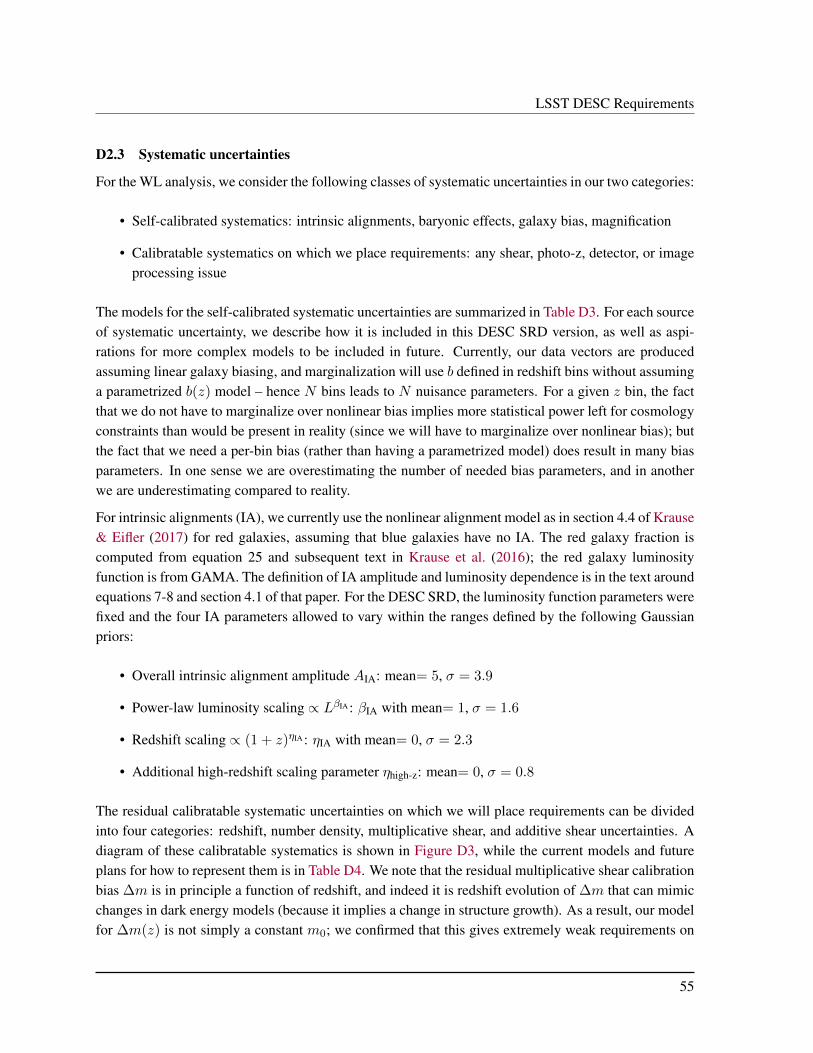
LSST DESC Requirements
D2.3 Systematic uncertainties
For the WL analysis, we consider the following classes of systematic uncertainties in our two categories:
• Self-calibrated systematics: intrinsic alignments, baryonic effects, galaxy bias, magnification
• Calibratable systematics on which we place requirements: any shear, photo-z, detector, or imageprocessing issue
The models for the self-calibrated systematic uncertainties are summarized in Table D3. For each sourceof systematic uncertainty, we describe how it is included in this DESC SRD version, as well as aspi-rations for more complex models to be included in future. Currently, our data vectors are producedassuming linear galaxy biasing, and marginalization will use b defined in redshift bins without assuminga parametrized b(z) model – hence N bins leads to N nuisance parameters. For a given z bin, the factthat we do not have to marginalize over nonlinear bias implies more statistical power left for cosmologyconstraints than would be present in reality (since we will have to marginalize over nonlinear bias); butthe fact that we need a per-bin bias (rather than having a parametrized model) does result in many biasparameters. In one sense we are overestimating the number of needed bias parameters, and in anotherwe are underestimating compared to reality.
For intrinsic alignments (IA), we currently use the nonlinear alignment model as in section 4.4 of Krause& Eifler (2017) for red galaxies, assuming that blue galaxies have no IA. The red galaxy fraction iscomputed from equation 25 and subsequent text in Krause et al. (2016); the red galaxy luminosityfunction is from GAMA. The definition of IA amplitude and luminosity dependence is in the text aroundequations 7-8 and section 4.1 of that paper. For the DESC SRD, the luminosity function parameters werefixed and the four IA parameters allowed to vary within the ranges defined by the following Gaussianpriors:
• Overall intrinsic alignment amplitude AIA: mean= 5, σ = 3.9
• Power-law luminosity scaling ∝ LβIA : βIA with mean= 1, σ = 1.6
• Redshift scaling ∝ (1 + z)ηIA : ηIA with mean= 0, σ = 2.3
• Additional high-redshift scaling parameter ηhigh-z: mean= 0, σ = 0.8
The residual calibratable systematic uncertainties on which we will place requirements can be dividedinto four categories: redshift, number density, multiplicative shear, and additive shear uncertainties. Adiagram of these calibratable systematics is shown in Figure D3, while the current models and futureplans for how to represent them is in Table D4. We note that the residual multiplicative shear calibrationbias ∆m is in principle a function of redshift, and indeed it is redshift evolution of ∆m that can mimicchanges in dark energy models (because it implies a change in structure growth). As a result, our modelfor ∆m(z) is not simply a constant m0; we confirmed that this gives extremely weak requirements on
55
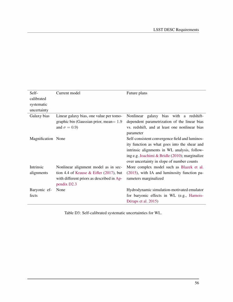
LSST DESC Requirements
Self-calibratedsystematicuncertainty
Current model Future plans
Galaxy bias Linear galaxy bias, one value per tomo-graphic bin (Gaussian prior, mean= 1.9
and σ = 0.9)
Nonlinear galaxy bias with a redshift-dependent parametrization of the linear biasvs. redshift, and at least one nonlinear biasparameter
Magnification None Self-consistent convergence field and luminos-ity function as what goes into the shear andintrinsic alignments in WL analysis, follow-ing e.g. Joachimi & Bridle (2010); marginalizeover uncertainty in slope of number counts
Intrinsicalignments
Nonlinear alignment model as in sec-tion 4.4 of Krause & Eifler (2017), butwith different priors as described in Ap-pendix D2.3
More complex model such as Blazek et al.(2015), with IA and luminosity function pa-rameters marginalized
Baryonic ef-fects
None Hydrodynamic simulation-motivated emulatorfor baryonic effects in WL (e.g., Harnois-Déraps et al. 2015)
Table D3: Self-calibrated systematic uncertainties for WL.
56

LSST DESC Requirements
m0 because, as noted previously by Massey et al. (2013), ∂C`/∂m0 differs significantly from ∂C`/∂w0
(orwa) when considering the full data vector ofC` across all redshift bins. In order to identify sensitivityof cosmological parameter constraints to multiplicative shear calibration uncertainties, it is important touse a redshift-dependent model; we adopted
∆m(z) = m0
(2z − zmax
zmax
)(6)
with zmax set to the middle of the highest tomographic redshift bin. Given this parametrization, the totalvariation in shear calibration across the redshift range used for the weak lensing analysis is 2m0, andrequirements on shear calibration should be interpreted as a requirement on our knowledge of redshift-dependent shear calibration trends across the sample. In principle, there is some higher-order depen-dence on the redshift-dependent function adopted, but do not explore this further in this version of theDESC SRD.
The DESC’s DC2 analysis effort will provide useful guidance on how to incorporate our need for knowl-edge of systematic uncertainty due to observational effects like airmass and PSF effects and how toconnect them to cosmological parameter estimates, so some models for inclusion of these effects andhow to place requirements on our knowledge of them (or associated scale cuts) are still to be defined infuture DESC SRD versions. Additional updates to our modeling might result from DC2- or DC3-eradecisions about whether the analysis will proceed in bins (which requires the calibration of photo-z’s ineach bin) or will rely on photo-z PDFs (in which case misspecification of PDFs may also be an issue,similar but not identical to catastrophic photo-z outliers in impact). In either case, a more sophisticatedmodel for the redshift-dependent photo-z bias, scatter, and outlier rate is needed.
It is worth noting that several of the effects listed in the right-most column of Figure D3 contribute tosystematic uncertainties for WL in several ways (number density, redshift, and shear-related uncertain-ties); it will be important to develop a self-consistent approach for how systematic uncertainties dueto blending, photometric calibration, galactic extinction, stars, galaxy characterization, selection bias,detector effects, and PSF modeling errors propagate into all of the observables.
Calibratable systematicuncertainty
Current model Future plans
Redshift uncertaintiesMean redshift Uncertainty in 〈z〉 for each to-
mographic binInvestigate bins separately
Redshift width A redshift bin width that is thesame for each bin modulo 1+
z factors
Account for inflation of σz at higher redshiftcompared to the 1 + z model; use DC2 guid-ance on σz
Catastrophic photo-z er-rors
None To be decided based on DC2
Galactic extinction None To be decidedPhotometric calibration None To be decided
57

LSST DESC Requirements
Blending None To be decidedNumber density uncertainties
Galactic extinction None To be decidedPhotometric calibration None To be decidedStars None Templates for incomplete detection near
bright stars, impact of bright stars on back-ground estimates, stellar contamination ofgalaxy sample, . . .
Airmass, PSF, other ob-servational effects
None To be decided based on DC2
Blending None To be decided based on DC2Shear (multiplicative) uncertainties
Blending None To be decided based on DC2Stars Fractional contamination of
galaxy sample by starsTo be decided based on DC2
Galaxy characterization None To be decidedGalaxy selection bias None To be decidedDetector effects None To be decided based on DC2PSF modeling errors PSF model size requirement
based on second momentsTo be decided based on DC2
Shear (additive) uncertaintiesBlending None To be decided based on DC2Galaxy characterization None To be decidedGalaxy selection bias None To be decidedDetector effects None To be decided based on DC2PSF modeling errors ρ statistics To be decided based on DC2Member galaxy contam-ination
None To be decided
Table D4: Calibratable systematic uncertainties for WL.
Finally, several boxes in the right-most column of Figure D3 implicitly include multiple effects. Forcompleteness, we note the primary contributors to these, which will eventually be important for model-ing their impact on the observable quantities:
• Detector effects: brighter-fatter, glowing edges, tree rings, and others.
• PSF modeling errors: differential chromatic refraction, chromatic seeing, other chromatic effectsin the optics and sensors, color gradients, relative astrometry between exposures, model bias, PSFinterpolation, contamination of the PSF star sample by binaries.
58

LSST DESC Requirements
3x2pt systematic uncertainties
Redshift
Shear (multiplicative)
Shear (additive)
Number density
Blending
Mean redshift
Redshift scatter
Photometric calibration
Catastrophic photo-z error
Galactic extinction
Detector effects
PSF modeling errors
Galaxy characterization
Galaxy selection bias
Stars
Airmass, PSF, other observational effects
Figure D3: Diagram indicating sources of systematic uncertainty for the WL analysis on which wewould like to place requirements in the DESC SRD. The direction of the arrows indicates the flowfrom overall systematic uncertainty to broad systematics categories to the specific physical effects onwhich we place requirements. As shown, there are several low-level issues in the right-hand columnthat contribute to multiple categories of uncertainty in the middle column. The green / lavender boxesindicate sources of uncertainty on which we do / do not place requirements in this DESC SRD version,respectively. The cyan boxes indicate those for which more R&D beyond the DESC’s DC2 may beneeded in order to place requirements. For some of the green boxes, we currently only have softwareinfrastructure to place requirements through their impact on one class of uncertainty; such connectionsare shown as green arrows.
59

LSST DESC Requirements
• Galaxy characterization: insufficient PSF correction method, pixel-noise bias, model bias
• Blending: effects on detection, astrometry, photometry, and shapes due to undetected blendedobjects, selection effects, increased model and/or noise bias
These may not be explicitly modeled independently in the end, but understanding the nature of thesecontributing factors may be important for building up templates for systematics.
D3 Galaxy clusters
For the purpose of this first version of the DESC SRD, the default galaxy cluster abundance analysisincorporates the cluster counts as a function of richness and redshift, along with stacked cluster weaklensing in the 1-halo regime to constrain parameters of the cluster mass-observable relation (MOR).
D3.1 Analysis choices
Here we describe the essential points of the CL analysis setup in this version of the DESC SRD. Itlargely follows the treatment in Krause & Eifler (2017), with a few variations:
• For the source sample, we use the same sample as defined for WL in Y1 and Y10. See Ap-pendix D2 for number densities, redshift distributions, tomographic bin definitions, and otherrelevant parameters.
• The cluster-shear data vector consists of the angular power spectra, C`, defined in redshift andrichness bins, along with the cluster counts on those bins N(λ, z).
• We use the same set of globally defined ` bins as described for the LSS analysis. Since the analysisfor now uses only the 1-halo regime, we restrict to 3 382 ≤ ` ≤ 15 000. The choice of lower` limit is due to technical issues in covariance estimation; lower ` values may be used in futureDESC SRD versions.
• The cluster-shear data vector is a stack of the Fourier transform of NFW profiles given the redshiftand mass distribution of the clusters and a concentration-mass relation from Bhattacharya et al.(2013). At high redshift, the lowest ` bins contain a contribution from the 2-halo term. Thisterm is constructed using the nonlinear matter power spectrum along with the halo bias vs. massrelation from Tinker et al. (2010). Currently the bias is fixed and is not fit for as a free parameter.
• Covariances are calculated following Krause & Eifler (2017).
• The cluster sample binning is defined as follows:
– λ = [20, 30], [30, 45], [45, 70], [70, 120], [120, 220]
– z = [0.2, 0.4], [0.4, 0.6], [0.6, 0.8], [0.8, 1.0] for Y10, with the highest redshift bin omittedin Y1 due to the shallower depth of the Y1 imaging data.
60

LSST DESC Requirements
• For the first version of the DESC SRD, we assume perfect knowledge of cluster redshift, i.e.,there is no photo-z error.
D3.2 Anticipated improvements
The above baseline analysis does not correspond to either cluster cosmology analysis approach thatis under consideration within the DESC. The clusters working group is considering two approaches,at least one of which should be included in a future DESC SRD version. The two approaches are asfollows:
• An extension of the approach described above to include cluster-shear correlations in the 2-haloregime, along with cluster-cluster correlations.
• An approach that involves using individual cluster shear profiles, rather than a stacked analysis.
In addition, external X-ray and SZ data will be used to place priors on certain astrophysical nuisanceparameters (MOR, optical cluster miscentering). A more direct connection to that data, given somereasonable assumptions about what will be available when the LSST survey starts, would be desirable –i.e., using sample sizes to connect to the size of the priors on the MOR parameters.
Additional extensions for consideration include stacking in real space using physical coordinates forbetter reconstruction of cluster profiles, going to lower `, and a comparison of stacking shear vs. surfacedensities.
D3.3 Systematic uncertainties
For the CL analysis, we consider the following classes of systematic uncertainties in our two categories:
• Self-calibrated systematics: mass-observable relation, intrinsic alignments, other theory uncer-tainties (e.g., mass function), cluster miscentering, cluster large-scale bias, baryonic effects oncluster halo profiles and mass function, projection effects
• Calibratable systematics on which we place requirements: any shear, photo-z, detector, or imageprocessing issue
The models for the self-calibrated systematic uncertainties are summarized in Table D5. For clusterabundance measurements, the MOR tends to be the dominant self-calibrated systematic uncertainty(and dominates over purely statistical uncertainties). For each source of systematic uncertainty, wedescribe how it is included in this DESC SRD version, as well as aspirations for more complex modelsto be included in future.
For the first version of the DESC SRD, we use the MOR from Murata et al. (2018) with an extension ofredshift dependence. Specifically, the mean relation is defined as
lnλ(M, z|A,B,C) = A+B ln
(M
Mpivot
)+ C ln (1 + z) , (7)
61

LSST DESC Requirements
and the mass-dependent mass-observable scatter is defined as
σlnλ|M (M, z|σ0, qM , qz) = σ0 + qM ln
(M
Mpivot
)+ qz ln (1 + z) . (8)
This is a slight update from Krause & Eifler (2017) where they used a constant mass-observable scat-ter. We assume fiducial values for A, B, and σ0 used in Murata et al. (2018), fiducial values 0for C, qm, and qz . The pivot mass is Mpivot = 3 × 10¹⁴h−1M. We use Gaussian priors forA and B with a width corresponding to 80% of the probability within the flat prior ranges for Aand B used in Murata et al. (2018) and a Gaussian prior with σ = 1.2 for C. For nuisance pa-rameters in the mass-observable scatter, we use priors which are not directly on these parametersbut on scatters at three different richnesses and redshifts, P (σlnλ|M (Mfid(λi, zi), zi|σ0, qM , qz)) =
Gauss[σlnλ|M (Mfid(λi, zi), zi|σ0,fid, qM,fid, qz,fid), σi], where σi = 0.1 and Mfid(λi, zi) is the inverseof the mean relation with the fiducial nuisance parameters; there are different sets of (λi, zi) and differ-ent assumptions about how well the scatter can be constrained for Y1 and Y10. The priors for Y1 andY10 are based on reasonable assumptions of ancillary datasets that will be available at those times:
• Y1: The constraints are√N extrapolations from current constraints of ∼10% on the scatter in
the mass-observable relation for N = 30 clusters. Based on this assumption, we use (λi, zi) =
(90, 0.2), (30, 0.1), and (100, 0.8), assuming the scatter in the MOR is known to 0.06, 0.05,and 0.04 respectively, corresponding to 100, 150, and 200 clusters. The 100 cluster assumptionis based on expectations for Chandra+SPT follow-up, the 150 cluster assumption is based onan already-completed observing program with Swift, and the 200 cluster assumption is fromcombined SPT+ACT.
• Y10: We use (λi, zi) = (80, 0.2), (30, 0.1), and (90, 0.8), assuming the scatter in the MOR isknown to 0.03, 0.05, and 0.03 respectively, corresponding to 500, 150, and 500 clusters, respec-tively. The 500 cluster assumption is based on expectations for eROSITA and CMB-S4, and isconservative for those surveys (but we assume there will be some systematics floor that preventsfurther constraint on scatter in the MOR even for higher N ). The 150 cluster assumption for lowredshift is based on an already-completed observing program with Swift.
The residual calibratable systematic uncertainties on which we will place requirements can be dividedinto four categories: redshift, number density, multiplicative shear, and additive shear uncertainties. Adiagram of these calibratable systematics is shown in Figure D4, while the current models and futureplans for how to represent them is in Table D6. The DESC’s DC2 analysis effort will provide usefulguidance on how to incorporate our need for knowledge of systematic uncertainty due to observationaleffects like airmass and PSF effects and how to connect them to cosmological parameter estimates, sosome models for inclusion of these effects and how to place requirements on our knowledge of them(or associated scale cuts) are still to be defined in future DESC SRD versions. It is worth noting thatseveral of the effects listed in the right-most column of Figure D4 contribute to systematic uncertaintiesfor CL in several ways (number density, redshift, and shear-related uncertainties); it will be important
62
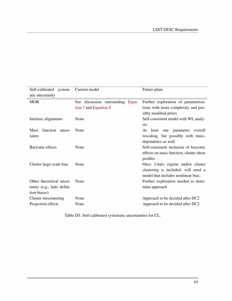
LSST DESC Requirements
Self-calibrated system-atic uncertainty
Current model Future plans
MOR See discussion surrounding Equa-tion 7 and Equation 8
Further exploration of parametriza-tions with more complexity and pos-sibly modified priors
Intrinsic alignments None Self-consistent model with WL analy-sis
Mass function uncer-tainty
None At least one parameter overallrescaling, but possibly with mass-dependence as well
Baryonic effects None Self-consistent inclusion of baryoniceffects on mass function, cluster shearprofiles
Cluster large-scale bias None Once 2-halo regime and/or clusterclustering is included, will need amodel that includes nonlinear bias.
Other theoretical uncer-tainty (e.g., halo defini-tion biases)
None Further exploration needed to deter-mine approach
Cluster miscentering None Approach to be decided after DC2Projection effects None Approach to be decided after DC2
Table D5: Self-calibrated systematic uncertainties for CL.
63

LSST DESC Requirements
to develop a self-consistent approach for how systematic uncertainties due to blending, photometriccalibration, galactic extinction, stars, galaxy characterization, selection bias, detector effects, and PSFmodeling errors propagate into all of the observables.
The parameters related to shear calibration, shear sample tomographic bins, and source photo-z areshared with the WL analysis (Appendix D2).
Calibratable systematicuncertainty
Current model Future plans
Redshift uncertaintiesMean redshift Uncertainty in 〈z〉 for each to-
mographic binInvestigate bins separately
Redshift width A redshift bin width that is thesame for each bin modulo 1+
z factors
Account for inflation of σz at higher redshiftcompared to the 1 + z model; use DC2 guid-ance on σz
Catastrophic photo-z er-rors
None To be decided based on DC2
Cluster photo-z errors None To be decidedGalactic extinction None To be decidedPhotometric calibration None To be decidedMember galaxy contam-ination
None To be decided
Number density uncertaintiesGalactic extinction None To be decidedPhotometric calibration None To be decidedBlending None To be decided based on DC2Stars None Templates for incomplete detection near
bright stars, impact of bright stars on back-ground estimates, stellar contamination ofgalaxy sample, . . .
Airmass, PSF, other ob-servational effects
None To be decided based on DC2
Member galaxy contam-ination
None To be decided
Shear (multiplicative) uncertaintiesBlending None To be decided based on DC2Stars Fractional contamination of
galaxy sample by starsTo be decided based on DC2
Galaxy characterization None To be decidedGalaxy selection bias None To be decidedDetector effects None To be decided based on DC2
64

LSST DESC Requirements
PSF modeling errors PSF model size requirementbased on second moments
To be decided based on DC2
Non-weak shear re-sponse and flexion
None To be decided
Shear (additive) uncertaintiesBlending None To be decided based on DC2Galaxy characterization None To be decidedGalaxy selection bias None To be decidedDetector effects None To be decided based on DC2PSF modeling errors ρ statistics To be decided based on DC2Member galaxy contam-ination
None To be decided
Table D6: Calibratable systematic uncertainties for CL.
Finally, we note that several boxes in the right-most column of Figure D4 implicitly include multipleeffects. The primary contributors to these are listed in Appendix D2.3. Where possible, adopting acommon approach to these systematics and their impact on LSS, WL, and CL would be desirable.
D4 Supernovae
D4.1 Analysis choices
Here we describe the essential points of the SN analysis setup in this version of the DESC SRD:
The surveys are simulated in four separate parts: a one-year DDF survey, a ten-year DDF survey, a ten-year WFD survey and an external low-redshift sample. For all simulations we use simulation librariesfrom Biswas et al. (2017) to take the OpSim minion_1016 run and provide inputs to the SuperNovaANAlysis (SNANA Kessler et al. 2009) software to generate supernova light curves. Then we fit thoselight curves with the SALT2 model (Guy et al. 2007; Betoule et al. 2014), and compute distance moduliusing the Marriner et al. (2011) approach. The analysis follows the prescription of Scolnic et al. (2018),which was most recently used for the Pantheon sample of supernovae.
These statements assume that a commissioning mini-survey will reach ‘template depth’ of 5-10 timesthe single night coadd depth of the DDF (around 3000s exposures) in the DDF regions to produce deeptemplates in order to detect SN from difference images in the first year of operation. In the absence ofsuch a mini-survey, the first year survey results should be considered to have significantly fewer SN34
– or, effectively, the first year forecasts actually describe our capabilities after 2-3 years rather than oneyear. Similarly, the first few years of observation of the wide field will be used to generate templates,hence we do not assume a WFD year-one survey, and restrict ourselves to those obtained after 10 years.
34This is not just because of the time to make the observations that will be used to build the templates, but because of theneed for a time lag to avoid the supernovae we want to measure being in the templates.
65

LSST DESC Requirements
CL
Redshift
Shear (multiplicative)
Shear (additive)
Number density
Blending
Mean redshift (src)
Redshift scatter (src)
Photometric calibration
Catastrophic photo-z error (src)
Galactic extinction
Cluster photo-z
Member galaxy contamination
Detector effects
PSF modeling errors
Galaxy characterization
Galaxy selection bias
Stars
Non-weak shear response
Airmass, PSF, other observational effects
Figure D4: Diagram indicating sources of systematic uncertainty for the CL analysis on which we wouldlike to place requirements in the DESC SRD. The direction of the arrows indicates the flow from overallsystematic uncertainty to broad systematics categories to the specific physical effects on which we placerequirements. As shown, there are several low-level issues in the right-hand column that contribute tomultiple categories of uncertainty in the middle column. The green / lavender boxes indicate sourcesof uncertainty on which we do / do not place requirements in this DESC SRD version, respectively.The cyan boxes indicate those for which more R&D beyond the DESC’s DC2 may be needed in orderto place requirements. For some of the green boxes, we currently only have software infrastructure toplace requirements through their impact on one class of uncertainty; such connections are shown asgreen arrows.
66

LSST DESC Requirements
The current software framework for forecasting cosmological constraining power with SNe and theimpact of systematics involves a sample of simulated Type Ia supernovae, with selection cuts, thatget passed through light curve fitters. The simulated SN analyses currently assume that the supernovaredshifts are being determined through spectroscopic follow-up of the host galaxies. Such spectroscopicfollow-up of hosts is considerably simpler than spectroscopic followup of active supernovae, as it doesnot need to be done during the few-week window when a supernova is bright. Also, several supernovahosts within a small patch of sky aggregated over time may be simultaneously followed up using suitablemulti-object spectrographs35.
250,000 fiber hours have been allocated on 4MOST for the 4MOST-TiDES observations of transients,SN hosts, and AGN reverberation mapping – with LSST being the primary source of transients. Theusage of that allocated time is being decided, with a view to target as many viable hosts as possible(including galaxies where the SN candidate is not obvious). 4MOST can reach a depth of r ∼ 22 with1-hour exposures, which corresponds to roughly z ∼ 0.4− 0.6 (in OzDES). This will cover the bulk ofthe wide-survey candidates. In future, it will be valuable to estimate how many of the WFD supernovaemay have redshifts from the DESI survey, but this is likely to be subdominant to the number that willbe acquired by 4MOST. For the purpose of this forecast we assume the redshifts in the DDF will comefrom Subaru (see below).
We reduce the full simulated sample to a subset which would have spectroscopic host informationassuming 20 nights of observing time with the Prime Focus Spectrograph on the Subaru telescope in theDeep Drilling Fields, which can reach i = 22.86 hosts, plus 250k fiber-hours with the 4MOST surveyspread over the WFD area, which can reach i = 22 with the maximum possible 6 visits per fiber. Thefraction of Type Ia supernovae at a given redshift which are expected to have hosts bright enough forspectroscopy based on the stellar mass/SFR/photometric redshift catalogs of Laigle et al. (2018) areshown in Figure D5. We note that a similar (same order of magnitude) amount of observing time onDESI in the DDFs could garner a comparable number of host redshifts, given that DESI has a largerFoV, compensating for its smaller collecting area. Hence there are two potential pathways to obtain hostredshifts for the DDF supernovae.
The restriction on fiber hours leads to a total restriction of 100k supernovae which we obtain by scalingthe overall efficiency curves until we obtain the 100k objects in the final sample (see the note on fittinglight curves below). For both surveys we also assume an 80% secure redshift rate given the S/N forthe assumed exposure times, and assuming that some time is spent obtaining redshifts for non-Ias andother objects (converting an initial estimate of 125k supernova candidates to 100k). In this forecast, weassume the supernovae without redshifts will not be used for cosmological constraints. Work is ongoingwithin the DESC to study both the impact of host photo-z contamination on the overall science FoM,including mis-identification of hosts, and the best practice for mitigating redshift error (Roberts et al.2017; Malz, Peters, Hlozek et al. in preparation36). It is worth noting that the dark energy task force
35Such follow-up, which is used in current photometric supernova surveys like DES and Pan-STARRS, might be easiest tocombine with needs of other working groups like photometric redshifts.
36https://github.com/aimalz/scippr
67

LSST DESC Requirements
(DETF) assumed a much larger sample of 400k photometric supernovae with an ‘optimistic photo-z’error. We restrict ourselves to the more conservative case described above.
The Foundation survey (Foley et al. 2018) will observe∼ 800 low redshift SNe by the time it completesthe survey in 2020. For the Y10 survey, we triple this number of low-redshift SNe, given the number oflow-redshift surveys (e.g. ZTF) that will be online and will yield impressive numbers of supernovae bythe end of the LSST Y10 survey. We include this sample by decreasing the error on the distance modulusin our final Y10 sample by
√3 for z < 0.05−0.1. This low-z sample is an essential anchor to the Hubble
diagram. For the low-z sample, we do not include here any individual calibration systematics for thedifferent samples and filters. Instead, we include the SALT2 calibration systematic and uncertainty inthe HST calibration which affects both low-z and LSST supernovae. Future versions of the DESC SRDshould factor in a reasonable level of calibration uncertainties for the external low-z sample, which willmildly change its constraining power.
The supernovae are then fit in two stages: the data are fit with light curve templates based on the SALT2model (Guy et al. 2007; Betoule et al. 2014). At this stage, detection quality cuts are applied, and thenumber of supernovae reduces slightly compared to the original simulated light curve points. There isa quality cut to restrict the number of objects that we would put fibers on (for host-z determination):we require objects to have three epochs that have signal-to-noise ratios in the nightly coadds of greaterthan five. An epoch here is based on a detection where the likelihood of detection follows an SNR-dependence as modelled by the Dark Energy Survey. The quality cut at this stage is to ensure that anyfibers used to obtain host galaxy spectra are placed on ‘high quality’ candidates.
The separate subsamples described above are then combined to form the overall Y1 and Y10 samplesas follow: DDF Y1 and an 800-SN low-z sample to form the overall Y1 sample; DDF Y10, a 2400-SNlow-z sample, and WFD Y10 sample to form the overall Y10 sample.
We apply the following quality cuts for inclusion of the SNe in the final cosmological sample: |c| <0.3, |x1| < 3, σ(x1) < 1, σ(t0) < 2, where c, x1, t0 are the color, stretch and explosion time respec-tively. Following the cuts on light curve fit quality, we arrive at a sample of ∼ 2400 SNe for the Y1sample, and ∼ 104000 SNe for the Y10 sample. The distance moduli are included as a likelihood inCosmoSIS37 (Zuntz et al. 2015), which makes use of algorithms for efficient sampling of cosmologicalparameter space (Lewis et al. 2000; Howlett et al. 2012).
The number of SNe obtained and their light curve quality depend strongly on the survey cadence. Initialstudies show that the total number of high-quality SNe in the 10-year survey can change by a factor of∼ 1.5 with cadences that are optimized for their detection, which will not only improve the statisticaluncertainty, but also allow for new studies of supernova systematics38.
For the WFD survey, the corresponding numbers depend even more strongly on the cadence strategyemployed. With that caveat, we obtain a final sample combining the WFD and DDF and low-z data of
37https://bitbucket.org/joezuntz/cosmosis/wiki/Home38Exploration of the impact of cadence on cosmology with SNe is a key ongoing DESC activity.
68

LSST DESC Requirements
0.0 0.5 1.0 1.5 2.0 2.5 3.0
redshift z
0.0
0.2
0.4
0.6
0.8
spec
trosc
opic
effic
ienc
y
WDF: 4MOST deep (6 visits)DDF: SUBARU (20 PFS nights)
Figure D5: Host spectroscopic redshift efficiencies for the WFD and DDF fields, assuming follow-upusing a combination of maximum-depth observations with the 4MOST survey (for WFD) and 20 nightsof observing time with the Prime Focus Spectrograph on the Subaru telescope (for DDF). The curvescorrespond to the fraction of Type Ia supernovae at a given redshift which have hosts bright enough tobe targeted for spectroscopy (corresponding to a limit of i = 22 for the maximum possible 6 visits with4MOST, or i = 22.86 for this Subaru survey). We place additional restrictions on the total number ofSNe that can be followed up with 4MOST, given the total allocation of 250k fiber-hours. In addition tothe losses from hosts too faint to target that are plotted here, we assume that 20% of targets will fail toyield highly-secure redshifts based on past experience with data of the expected S/N.
69

LSST DESC Requirements
∼112 000 SNIa with sufficiently well-sampled light curves, host galaxy redshifts, with a distributionpeaking around z ∼ 0.4. The WFD and low-z sample significantly improve the SN science case for thefollowing reasons:
• The resulting low-redshift sample is complete up to z ∼ 0.4, which adds significantly to thequality of the Hubble diagram constraints.
• z < 0.5 is roughly the redshift range where BAO is limited by cosmic variance. An all-skyz . 0.5 SN sample over ten years is unique as a distance indicator in this region. Further, wenote that there is no other SN survey capable of producing a sample of around 100 thousandsupernovae.
• A rolling cadence or other more optimal cadence may substantially increase the number of SNewith well-sampled light curves, allowing us to reach the nominal statistics in a fraction of theduration of the survey (modulo uncertainties in the host redshift), and providing a larger samplewith which to study systematic effects. It may also enable the construction of a deeper supernovasample, extending the redshift lever arm for this probe.
• The low-redshift sample will also be useful both in constraining non-standard cosmological mod-els and improving our understanding of the SN population and underlying correlations with envi-ronments. Moreover, it allows for the opportunity of probing structure growth with supernovae.
In contrast, the deep drilling fields will generate a superb ‘gold’ sample of supernovae out to z ∼ 1.2,
which not only allow for cosmological constraints, but will enable us to study the redshift evolution ofsupernova systematics (e.g., evolution of SN populations).
D4.2 Anticipated improvements
In future DESC SRD versions, we believe we can improve both the precision and accuracy of supernovacosmology with several changes to the baseline analysis presented here. These new approaches arestill a subject under development, and the tradeoff in terms of quantitative success versus additionalcomputational cost will determine which approaches are adopted in the end. We present a brief outlineof such newer analysis methods below:
1. Standardization of supernova light curves: Historically, supernova cosmology has used a two-step standardization approach of (a) compressing SNIa light curves into a universal function ofa few light curve model parameters thereby dimensionally reducing the multi-band time seriesdataset, and then (b) using a correlation between these light curve model parameters to an intrinsicbrightness or distance of the supernova. Currently, surveys use models (Guy et al. 2007) whichinclude a scatter∼ 0.1 mags in the resultant redshift-distance relationship, part of which correlateswith the environment of the supernova, potentially leading to biases in cosmological analysis.
70

LSST DESC Requirements
Following current standard approaches, the baseline analysis tries to account for this via post-facto correctional terms based on host galaxy stellar mass, and an attempt to distribute the scatterin the different model parameters. A better approach that minimizes the intrinsic dispersion andaccounts for such environmental dependence in training the model itself requires the developmentof newer SN light curve models (Kim et al. 2013, 2014; He et al. 2018), which is a key projectin the SRM. These more sophisticated models will also make it possible to incorporate redshiftdependencies of the components of the models, which presumably are primarily related to theenvironmental correlations with redshift (known and unknown).
2. Supernova selection: The selection criteria for the supernova sample in the baseline analysis isdesigned to yield a sample which has a small impurity of moving objects. While this might havea small impact on surveys designed for SN cosmology, it is possible that this choice has a largeimpact on the supernova sample for a multipurpose survey like LSST. Therefore, we would liketo investigate the possibility of less aggressive selection combined with a more computationally-intensive filtration step to a sample purity similar to the current strategy. For certain observingstrategies, this could result in an increase in good quality supernovae in the final cosmologicalsample.
3. Cosmology Inference: The current baseline analysis uses a method of estimating the distancemodulus (Marriner et al. 2011) and intrinsic dispersion which has been validated on SDSS data,and compares binned theoretical and ‘observed’ values of distance moduli for supernovae binnedin redshift. In the future, we would like to better model the relationships between different pa-rameters used in the cosmological inference (e.g. Hinton et al. in preparation39), including thesystematic parameters, leading to a likelihood of a large number of parameters. An importantfeature of these methods is that they enable better treatment of systematics, leading to betterknowledge of them after the analysis. A problem with these methods is the integration with otherprobes in the joint likelihood analysis (e.g. with TJP tools due to software and parallelizationissues).
4. Photometric Classification and Cosmological Inference: The current baseline analysis assumesthat (binary) photometric classification (using PSNID; Sako et al. 2011; Campbell et al. 2013)is performed accurately. In practice, any photometric classification algorithm will mis-classifyobjects, causing biases. This can be accounted for using algorithms like BEAMS (Hlozek et al.2012; Jones et al. 2017) in the future. Further, we plan to study the extension of cosmologi-cal inferences with photometric classification to include supernovae whose host redshifts are notknown (Roberts et al. 2017; Malz, Peters, Hlozek et al. in preparation40).
5. Cross-correlations between probes: Some of the systematic effects that affect the supernova sci-ence case can be mitigated by cross correlating supernova with other probes, and indeed can
39http://dessn.github.io/sn-doc/doc/out/html/index.html40https://github.com/aimalz/scippr
71

LSST DESC Requirements
mitigate the systematics of other probes. For example, measurements of the LSST SN magnifi-cations could be used to calibrate multiplicative errors in the LSST cosmic shear measurements(Zhang 2015), while measurements of the skewness and kurtosis of the SN magnitude distribution(see Macaulay et al. 2017) will help constrain σ8. Further study of the impact of systematics onthese cross-correlations will be an important area of research and development with DC2 data andbeyond.
6. Retraining the SALT2 model: SN4 shows that it is essential to retrain the SALT2 models as partof the analysis. Also, doing this retraining simultaneously with the cosmology inference has thepotential to add constraints on filter wavelength calibration.
On a more technical note, non-Gaussian contours in cosmological parameter space may need to be morefully addressed in future DESC SRD versions; they were neglected in this one.
The issue of redshift uncertainty and its impact on the supernova science case is an active area of studywithin the DESC SNWG. In this analysis we assume the existence of host spectroscopic redshifts for allsupernovae that form part of the final sample. In the next iteration of the DESC SRD, we will deviatefrom this default, by also assuming a simple photo-z model for the majority of objects. This subsamplewill again be selected with an efficiency that roughly matches expected spectroscopic redshift yield.This source of systematic uncertainty is one of the most important ones to model in the future, as thisaffects both axes on the Hubble diagram (µ fits in addition to z).
In this analysis, we have also made a large simplifying assumption that the cosmology sample consistsof only Type Ia supernovae that have been selected with perfect efficiency and purity. The potentialbias from misclassification (so-named classification uncertainty), will be introduced in the future byincluding some percentage (a few percent, given reasonable estimates of classification purity, see e.g.Campbell et al. 2013) of non-Ias for which the light curves get fit as if they were Ias, and checking theinduced bias. This results in a conservative requirement that ignores improvements that can be gainedfrom probabilistic inference methods (e.g., Roberts et al. 2017), and would represent our ‘worst case’scenario for classification bias.
D4.3 Systematic uncertainties
For the SN analysis, we consider the following classes of systematic uncertainties in our two categories:
• Self-calibrated systematics: astrophysical systematics (errors in the modelling of SN and theirstandardization based on the supernova light curve, the environment, and any other redshift de-pendencies,including those induced by weak lensing magnification and peculiar velocities)
• Calibratable systematics on which we place requirements: calibration (uncertainty on filter zeropoints, the transmission function wavelength, wavelength-dependent flux calibration, uncertain-ties in Galactic extinction corrections); redshift uncertainty; detection, classification
72

LSST DESC Requirements
The models for the self-calibrated systematic uncertainties are summarized in Table D7. For each sourceof systematic uncertainty, we describe how it is included in this DESC SRD version, as well as aspi-rations for more complex models to be included in the future. Generally speaking, the systematic un-certainties are estimated by simulating the supernova sample with the given systematic effect includedand comparing the distance modulus to the case where no systematic is included. This difference inthe distance modulus redshift-by-redshift produces a systematics covariance matrix for each systematic,which is added to the intrinsic scatter. In these cases, the systematic uncertainty is naturally estimatedas a data covariance (µ estimates) and then propagated into cosmological parameter space.
We assume that the error in the intrinsic dispersion modelling will be reduced by two times its currentvalue given the large sample of SNe in the full survey that can be used to study the scatter, in combi-nation with spectra from the ground-based collaboration. Similarly, for the host mass-SN luminositycorrelations, a bias in the high-mass sample following the model from Hounsell et al. (2017) is intro-duced into the simulations and ignored in the fitting, and this is used to estimate the resulting systematicuncertainty.
We introduce a SN-color population drift (again following the prescription in Hounsell et al. 2017) thatgets ignored in the fitting to determine the systematic uncertainty. Finally, we include a systematicdue to the potential from evolution of the β SALT2 parameter which describes the colour-luminositycorrelation, which we include as half of the measurement uncertainty of dβ/dz as determined from oursimulated LSST sample, because we can take the average of the observed and expected values.
Self-calibrated system-atic uncertainty
Current model baseline Future plans
Standardization of color-luminosity law and its z-dependence
Marginalization over SALT-II pa-rameter β Scolnic et al. (2014) athalf the predicted measurement un-certainty
Same as current model
Intrinsic scatter Modelling differences between Guyet al. (2010) and Chotard et al.(2011) at half model differences
To be decided
Host mass-SN luminos-ity correlations
High-mass sample bias as in Houn-sell et al. (2017)
To be decided
Magnification-inducedcovariances (especiallyfor DDFs)
Not modeled To be decided
Individual low-z calibra-tion uncertainty
Not modeled To be decided
Table D7: Self-calibrated systematic uncertainties for SN.
73

LSST DESC Requirements
The residual calibratable systematic uncertainties on which we will place requirements can be dividedinto 3 categories: calibration, redshift, and identification-related systematic uncertainties. A diagram ofthese calibratable systematics is shown in Figure D6, while the current models and future plans for howto represent them is in Table D8.
The DESC’s DC2 analysis effort will provide more sophisticated models for the impact of several ofthese effects than the ones used in these simulations.
SN systematic uncertainties
Calibration
Redshift
Identification
Filter zeropoints
Filter mean wavelengths
Filter variation across FOV
SN light curve modeling
Nonlinearity
Wavelength-dependent flux calibration
MW extinction corrections
Classification
Figure D6: Diagram indicating sources of systematic uncertainty for the SN analysis on which we wouldlike to place requirements in the DESC SRD. The direction of the arrows indicates the flow from overallsystematic uncertainty to broad systematics categories to the specific physical effects on which we placerequirements. The green boxes indicate sources of uncertainty on which we place requirements in thisDESC SRD version, respectively. In some cases, as discussed in Table D8, the systematics models willhave to be updated.
One might expect systematic errors to be correlated (for example the filter mean wavelengths and cutoffpositions). Here we have assumed that all systematics can be varied individually, and estimated the
74

LSST DESC Requirements
Calibratable systematicuncertainty
Current model baseline Future plans
CalibrationFilter zero points N (0, 1 mmag) offset per
bandSame as current model
Filter mean wavelength N (0, 1 ) Same as current modelFilter variation acrossFOV
None 10 measurements across FoV with 5 Å meanwavelength uncertainty
SN light curve modeling One-third scaling of Betouleet al. (2014) SALT2 parame-ter covariance matrix
Same as current model
Nonlinearity None 3 mmag over 5 magWavelength-dependentflux calibration
5 mmag slope over 7000 Å Same as current model
MW extinction correc-tions
5% scaling of Schlafly et al.(2014) model
Same as current model
RedshiftRedshift None To be included based on DC2
IdentificationClassification None To be included based on DC2 or DC3
Table D8: Calibratable systematic uncertainties for SN. The numbers given in the table represent a basevalue for the level of uncertainty; the requirements given in Section 5.4 were placed using contaminateddata vectors with various multiples of this best guess. Note that the ‘base’ value of the systematics waschosen as larger than our intended baseline, in order to fully investigate the systematics requirements.
75

LSST DESC Requirements
impact of them separately. For the band-dependent systematics we then include their combined con-tribution through a Monte Carlo simulation of the individual bias vectors. This allows for the separateuncertainties for different bands.
Finally, we note that the extinction requirement is placed without allowing for uncertainty in the MilkyWay dust law, which is yet another layer of complexity with the potential to introduce apparent differ-ences between low- and high-redshift supernova populations. We defer consideration of this effect tofuture versions of the DESC SRD.
D5 Strong lensing
D5.1 Analysis choices
Here we describe the essential points of the SL analysis setup in this version of the DESC SRD:
The Y10 strong lensing sample for our baseline analysis consists of time delay systems and compoundlenses. The time delay cosmography sample is defined as 400 lensed quasar systems monitored withLSST through 2032 and followed-up with TMT/GMT/JWST/E-ELT, so as to provide a 7% time delaydistance measurement after marginalization over lens model parameters (including lens galaxy massdistribution, environment and line of sight structure). This marginalization is implicit, not explicit.The sample size was estimated using OM10 predictions41 (Oguri & Marshall 2010) and results of theDESC’s Time Delay Challenge, with requirements on length of the time delay, image separation, andability to obtain follow-up data.
The Y10 compound lens sample is assumed to include 87 double source plane lenses. This calcu-lation uses LensPop42 (Collett 2015) modified to include compound lenses using best seeing singleepoch imaging alone. Thus all systems are bright enough that follow up is practicable. We assumethat each is followed up with TMT/GMT/JWST/E-ELT so as to provide fractional precision on β of[(0.01/Rein,1)2 + (0.01/Rein,2)2 + 0.012
]1/2 after marginalization over lens model parameters.
For Y1, lensed quasars are challenging due to the need to generate high-quality template imaging thatcan be used as a reference for identifying time-varying objects in the first ∼ 2 years of the survey. Asfor supernovae, we assume that a commissioning mini-survey may result in templates being availableslightly earlier than would otherwise be possible. We assume 20 of the brightest and most variablelenses will get measured time delays early. We can, however, reliably assume there will be of order tencompound lenses in Y1.
In both Y1 and Y10, the likelihood function is taken as gaussian in Ddt for time delay lenses (norequirement on DA from lens velocities). For compound lenses the likelihood is taken as Gaussian.
These forecasts assume 1 high resolution image per lens (space or AO), and spectroscopic redshiftsfor lens and source in each system. In Najita et al. (2016), it was estimated that adaptive optics IFUspectroscopy for characterizing lens galaxy velocity dispersions and image positions for 100 strong lens
41https://github.com/drphilmarshall/OM1042https://github.com/tcollett/LensPop
76

LSST DESC Requirements
systems would require roughly 100 hours on GSMTs in total (or greater amounts of time on 8-10mtelescopes). Given the relatively modest requirements when spread out over a number of years, wetherefore assume that the needed spectroscopy will be done. As a backup plan, WFIRST or Euclidcould provide some of the high-resolution imaging.
D5.2 Anticipated improvements
This version of the DESC SRD does not include lensed supernovae in the forecasts, because of theadditional need for high-resolution cadenced imaging. Further developments with respect to follow-uptelescope resources may lead to their inclusion in the future. We anticipate that the Y10 sample couldinclude 50-500 lensed SNe systems (strongly dependent on follow-up resources), each providing a 5%time delay distance measurement after marginalization over lens model parameters.
There are also∼3500 lensed quasars that could yield precise time delays with supplementary data pointson their light curves. There are up to 2000 fainter compound lenses that are discoverable with LSSTcoadds. Exploiting these fainter systems will require significantly more high-resolution imaging time,and hence we defer consideration of these additional systems for the future.
D5.3 Systematic uncertainties
For the SL analysis, we consider the following classes of systematic uncertainties in our two categories:
• Self-calibrated systematics: lens model assumptions (lens galaxy mass distribution), environmenteffects (including halo vs. stellar mass relation), line-of-sight structure, compound lensing indouble source plane
• Calibratable systematics on which we will eventually place requirements: time delay measure-ment systematics, selection bias, photometry issues including blending, photo-z and M∗ errors inenvironment analysis
Currently the self-calibrated systematics are all included implicitly in the forecasts through adoptionof a larger uncertainty in distance estimates than are obtained from statistical error in the time delaymeasurements. Future work within the DESC will include a more physical forward-modeling of theseeffects and their impact on dark energy observables.
Developing models for how the calibratable systematics enter the observable quantities for LSST (specif-ically through challenges in time delay estimation or sample characterization) will be an important taskfor the DESC SL working group during DC2 and DC3. In this DESC SRD version, in the absence ofsuch models, no requirements will be placed for the SL analysis.
77

LSST DESC Requirements
E Synthesis of systematic uncertainties across all probes
E1 Systematic uncertainties in this DESC SRD version
In this section, we synthesize the list of systematic uncertainties on which requirements are placed inthis DESC SRD version (see Table E1). As in the appendices on individual probes, we divide theminto categories (e.g., uncertainties in redshifts, number densities, and so on). The top two categories areconsidered only for probes of structure growth, while the last is considered only for SN.
Systematic uncertainty Probes NoteRedshift uncertainties
Mean redshift LSS, WL, CL For CL, only source redshift un-certainties were considered
Redshift scatter LSS, WL, CLShear (multiplicative) uncertainties
Overall multiplicative bias WL, CL This requirement encompassesall sources of multiplicative bias
Stellar contamination WL, CL Subset of “Overall multiplicativebias”
PSF modeling errors WL, CL Subset of “Overall multiplicativebias”
Photometric calibration uncertaintiesFilter zeropoints SNFilter mean wavelengths SNWavelength-dependent flux calibration SNLight curve modeling SNMW extinction corrections SN
Table E1: List of all sources of systematic uncertainty for which we place requirements in this versionof the DESC SRD.
E2 Systematic uncertainties deferred for future work
In this DESC SRD version, we have focused on a limited list of systematic uncertainties for which thereis a clear prescription for describing how they modify the observable quantities for dark energy analy-sis. More complete wish-lists for calibratable systematic uncertainties on which requirements could beplaced in future may be found for each probe in Appendix D. More generally, as the DESC’s analysispipelines are constructed and models for systematics characterization and mitigation are built, intercon-nections between classes of uncertainties should be noted. For example, if a given effect could resultin systematic uncertainty in both redshift and number densities, a self-consistent model for those un-
78

LSST DESC Requirements
certainties should be built. Similarly, self-consistent models should be built for how a given systematicuncertainty affects the observables in different cosmological probes.
As described in Section 2, the choice not to place requirements on model-sufficiency for either type ofsystematic uncertainty may also be revisited in future DESC SRD versions.
While not strictly a systematic uncertainty, one issue affecting all probes that is important for fulfillingour high-level objectives (O3) and requirements (RH4) is the development of blinding methods thatwork at the level needed for single and joint probe analysis.
F Defining number densitiesFor the WL, LSS, and CL analyses, we need to define Y1 and Y10 source galaxy number densitiesand redshift distributions. LSS and WL also require number densities and redshift distributions for thephotometric lens sample. Older estimates, e.g., in the LSST Science Book (LSST Science Collaboration2009), used the best deep ground-based data and spectroscopic redshift samples available at the time.We would like to confirm these estimates for Y10 using more recent datasets, and produce a Y1 estimate.
Below we derive the photometric sample number density (Appendix F1), the source sample numberdensity (Appendix F2), the photometric sample redshift distribution (Appendix F3), and the sourcesample redshift distribution (Appendix F4). These numbers are somewhat different than common as-sumption on LSST densities found in the LSST science book based on updates in our understandingboth in observations and simulations, as will be described in detail in each subsection.
F1 Photometric sample number density
To estimate the overall galaxy number density for a photometric sample with a given flux limit, weuse the HSC43 Deep field i-band catalogs from the HSC Survey Public Data Release44 1 (Aihara et al.2018). This sample is useful because it requires relatively minimal extrapolation to LSST depths, is alarge enough field that cosmic variance is not too significant, and the bandpass is similar to the expectedLSST i-band.
The HSC data were downloaded with an SQL query that was designed to get a complete galaxy samplethat goes as deep as possible, with only minimal flag cuts (e.g., star/galaxy classification, only primarydetections, and nothing with saturated/interpolated pixels near the center of the galaxy). A bright starmask was imposed. Random points were also downloaded from the HSC deep database while imposingthe same flag cuts, in order to properly calculate the area45.
Using the random points, we calculated the area as 26.1 deg2. Note that this includes a∼12% reductionfactor for masks due to various image defects, bright stars, and so on. The number densities we calculate
43http://hsc.mtk.nao.ac.jp/ssp/survey/44https://hsc-release.mtk.nao.ac.jp/doc/45The real and random SQL queries can be found in the Requirements repository, ‘number_density/hsc.sql’ and ‘num-
ber_density/hsc_rand.sql’. The script that used the resulting HSC catalogs to carry out the calculations described below andmake Figure F1 is ‘number_density/dndmag_hsc.py’.
79
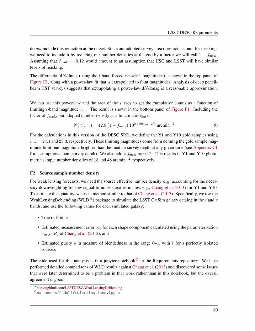
LSST DESC Requirements
do not include this reduction at the outset. Since our adopted survey area does not account for masking,we need to include it by reducing our number densities at the end by a factor we will call 1 − fmask.Assuming that fmask = 0.12 would amount to an assumption that HSC and LSST will have similarlevels of masking.
The differential dN /dmag (using the i-band forced cmodel magnitudes) is shown in the top panel ofFigure F1, along with a power-law fit that is extrapolated to faint magnitudes. Analysis of deep pencil-beam HST surveys suggests that extrapolating a power-law dN /dmag is a reasonable approximation.
We can use this power-law and the area of the survey to get the cumulative counts as a function oflimiting i-band magnitude ilim. The result is shown in the bottom panel of Figure F1. Including thefactor of fmask, our adopted number density as a function of ilim is
N(< ilim) = 42.9 (1− fmask) 100.359(ilim−25) arcmin−2 (9)
For the calculations in this version of the DESC SRD, we define the Y1 and Y10 gold samples usingilim = 24.1 and 25.3, respectively. These limiting magnitudes come from defining the gold sample mag-nitude limit one magnitude brighter than the median survey depth at any given time (see Appendix C1for assumptions about survey depth). We also adopt fmask = 0.12. This results in Y1 and Y10 photo-metric sample number densities of 18 and 48 arcmin−2, respectively.
F2 Source sample number density
For weak lensing forecasts, we need the source effective number density neff (accounting for the neces-sary downweighting for low signal-to-noise shear estimates; e.g., Chang et al. 2013) for Y1 and Y10.To estimate this quantity, we use a method similar to that of Chang et al. (2013). Specifically, we use theWeakLensingDeblending (WLD46) package to simulate the LSST CatSim galaxy catalog in the i and rbands, and use the following values for each simulated galaxy:
• True redshift z,
• Estimated measurement error σm for each shape component calculated using the parameterizationσm(ν,R) of Chang et al. (2013), and
• Estimated purity ρ (a measure of blendedness in the range 0–1, with 1 for a perfectly isolatedsource).
The code used for this analysis is in a jupyter notebook47 in the Requirements repository. We haveperformed detailed comparisons of WLD results against Chang et al. (2013) and discovered some issuesthat were later determined to be a problem in that work rather than in this notebook, but the overallagreement is good.
46https://github.com/LSSTDESC/WeakLensingDeblending47notebooks/RedshiftDistributions.ipynb
80

LSST DESC Requirements
20 21 22 23 24 25 26 27 28i-band magnitude
103
104
105
106
107
dN
/dm
ag [
deg−
2 m
ag−
1]
HSC deep: dlog10(N)/dmag=0.359
HSC Deep
CatSim
HSC fit
22.0 22.5 23.0 23.5 24.0 24.5 25.0 25.5 26.0 26.5i-band magnitude limit
101
102
Cum
ula
tive n
um
ber
densi
ty [
arc
min−
2]
HSC Deep, fit N(<ilim) = 42.9 100.359(ilim−25)
Figure F1: Top: The differential distribution of i-band galaxy magnitudes in the HSC Deep survey.Before the turnover due to incompleteness, the data (red solid curve) were fit to a power-law, shown as ared dotted line, with a slope indicated in the plot title. Finally, the dN /dmag in the CatSim catalog usedfor WeakLensingDeblending simulations (described in more detail in Appendix F2) is shown in black.Bottom: The cumulative number density of galaxies as a function of i-band limiting magnitude ilim. Thepower-law fit to the differential counts from the left panel was used to get an extrapolated version of thecumulative counts, shown as a dashed line. Vertical lines show the Y1 and Y10 limits of the photometricsample used for clustering analysis, as described in Appendix F1. The power-law equation is shown inthe plot title.
81

LSST DESC Requirements
We are interested in different sample definitions using:
• Y10 or Y1, where Y1 is defined as 0.1 of the total exposure time in each band for the purposes ofWLD simulations.
• The combined i+r sample or else i and r individually. For the combination, we use only galaxiesdetected in both bands and define the combined σ−2
m,i+r = σ−2m,i + σ−2
m,r.
• A weak-lensing sample selected using σm < k · σSN with k = 1 (nominal), 0.5 (conservative) or2.0 (optimistic). We fix σSN = 0.26 for this cut.
• With or without blending corrections. Blending reduces ν, which in turn reduces σm(ν,R), andthereby the selection fraction and the neff weight. We also remove galaxies with ρ < ρmin fromthe sample, assuming that they are too blended for reliable photo-z and shear estimation.
Table F1 summarizes the results with k = 1. Note that our treatment of blending effects is not par-ticularly conservative: we assume that all galaxies below a certain overlap fraction (ρmin = 0.85) areunusable and all other galaxies are optimally deblended.
Epoch Bands Blended n neff
Y10 i+ r Y 34.091 27.737Y10 i+ r N 41.765 34.581Y10 i Y 25.658 20.732Y10 i N 32.557 26.562Y10 r Y 26.594 21.402Y10 r N 34.319 27.922Y1 i+ r Y 13.969 11.112Y1 i+ r N 16.174 13.052Y1 i Y 10.230 8.051Y1 i N 12.317 9.744Y1 r Y 10.402 8.170Y1 r N 12.622 10.024
Table F1: Summary of results with k = 1. The last two columns give the integrated densities n(z) andneff(z), respectively, in units of galaxies per square arcminute. These densities are not corrected for anymasking effects. The scenarios that we use for forecasts are shown in red.
F3 Photometric sample redshift distribution
While the photometric sample number density as a function of limiting magnitude can be obtained fromHSC, this is not possible for the redshift distributions, due to the lack of redshift information in HSC.
82

LSST DESC Requirements
Hence we derive redshift distributions from the CatSim input catalog used for WLD, with a strict i-band limit as for the photometric samples discussed in Appendix F1. As a sanity check, they werecompared against parametric fits to spectroscopic redshift distributions estimated using DEEP248 data,correcting for the impact of selection/color cuts using the targeting weighting factors. The data onlyinclude redshifts up to z ∼ 1.4, so the redshift distribution beyond that is an extrapolation. In addition,DEEP2 is limited to R < 24.1, so the distribution is extrapolated to fainter magnitudes as well.
The comparison between the input catalog to WLD, our best-fitting parametric distribution in Equa-tion 5, and the best-fitting DEEP2 distribution49 is shown for Y1 and Y10 in Figure F2. As shown, theresults for z . 1.4 (where less extrapolation is required) agree quite well between CatSim and DEEP2.
F4 Source sample redshift distribution
The jupyter notebook mentioned in Appendix F2 saves the n(z) and neff(z) distributions for each rowof Table F1 to a subdirectory notebooks/neff/ using plain text format and a file name based onthe first three columns. Figure F3 has several panels comparing the resulting neff distributions to showthe impact of different choices (Y1 vs. Y10, blending, single band vs. both).
The resulting neff(z) (histograms and parametric fits) are shown for Y1 and Y10 in Figure F4.
G Forecasting-related plots
In this section, we collect a subset of representative plots from the forecasts:
• Figure G1 illustrates the main steps involved in the error budgeting process described at the startof Section 5.
• Figure G2 shows the (w0, wa) constraints from all five probes individually, and the joint forecastincluding Stage III priors as well50.
• Figure G3 shows how requirements were set for the calibratable systematic uncertainties for thesupernova analysis.
48http://deep.ps.uci.edu/49See ‘number_density/dndz.py’ in the Requirements repository.50Figure G2 was produced using ChainConsumer (Hinton 2016), with advice and support provided by the ChainConsumer
team.
83

LSST DESC Requirements
0.0 0.5 1.0 1.5 2.0 2.5 3.0z
0
1000
2000
3000
4000
5000ilim < 24.1
WLD, ⟨z⟩=0.92
DEEP2, ⟨z⟩=0.79
Fit: z2e−(z/0. 26)0. 94
0.0 0.5 1.0 1.5 2.0 2.5 3.0z
0
2000
4000
6000
8000
10000
12000ilim < 25.3
WLD, ⟨z⟩=1.08
DEEP2, ⟨z⟩=0.94
Fit: z2e−(z/0. 28)0. 90
Figure F2: The redshift distribution for the Y1 (top) and Y10 (bottom) photometric sample used forclustering, as predicted based on the CatSim input catalog used by WLD, a parametric fit to that dataused in Appendix D2, and DEEP2 (parametric fit based on data to z = 1.4 only).
84

LSST DESC Requirements
0.0 0.5 1.0 1.5 2.0 2.5 3.0 3.5 4.0Redshift
0.0
0.5
1.0
1.5
2.0
2.5
n eff(z
) [/s
q.ar
cmin
./z
=0.
1]
Y10Y1
0.0 0.5 1.0 1.5 2.0 2.5 3.0 3.5 4.0Redshift
0.0
0.5
1.0
1.5
2.0
2.5
3.0
n eff(z
) [/s
q.ar
cmin
./z
=0.
1]
No blendingBlended
0.0 0.5 1.0 1.5 2.0 2.5 3.0 3.5 4.0Redshift
0.0
0.5
1.0
1.5
2.0
2.5
n eff(z
) [/s
q.ar
cmin
./z
=0.
1]
i+rir
Figure F3: Top: The effective k = 1 redshift distribution for the Y10 and Y1 samples of i+r, includingthe effects of blending. Middle: The effective k = 1 redshift distribution for the Y10 i+ r sample, withand without including the effects of blending. Bottom: The effective k = 1 redshift distribution for theY10 samples in i+ r, i and r, including the effects of blending.
85

LSST DESC Requirements
0.0 0.5 1.0 1.5 2.0 2.5 3.0 3.5 4.0z
0.0
0.2
0.4
0.6
0.8
1.0
1.2
1.4Y1: neff = 9.52 / arcmin2
WLDeblending, mean=0.85Fit: z^2 Exp[-(z/0.13)^0.78]
0.0 0.5 1.0 1.5 2.0 2.5 3.0 3.5 4.0z
0.0
0.5
1.0
1.5
2.0
2.5Y10: neff = 26.94 / arcmin2
WLDeblending, mean=1.05Fit: z^2 Exp[-(z/0.11)^0.68]
Figure F4: The effective redshift distribution neff(z) for the Y1 (top) and Y10 (bottom) source samplefrom WLD, and a parametric fit to that data used in Appendix D2.
86
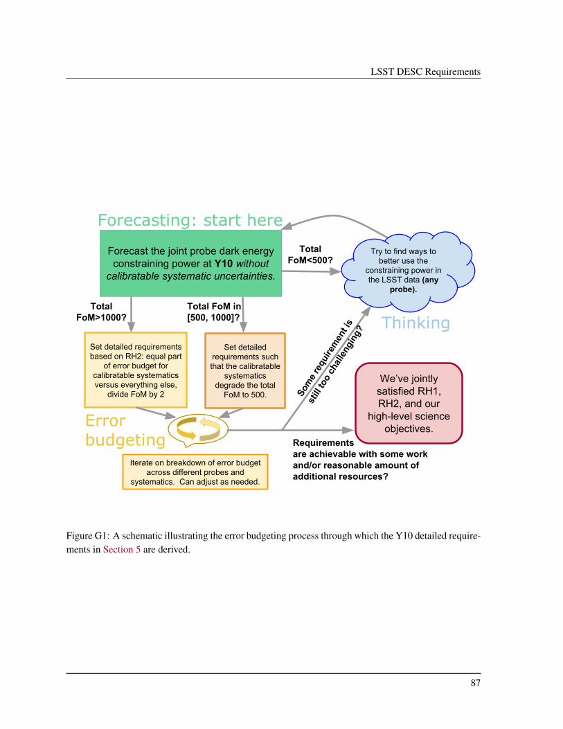
LSST DESC Requirements
TotalFoM<500?
Forecast the joint probe dark energy constraining power at Y10 without
calibratable systematic uncertainties.
TotalFoM>1000?
Total FoM in [500, 1000]?
Set detailed requirements based on RH2: equal part
of error budget for calibratable systematics versus everything else,
divide FoM by 2
Set detailed requirements such that the calibratable
systematics degrade the total
FoM to 500. Som
e req
uire
men
t is
still
too
chall
engi
ng?
Requirements are achievable with some work and/or reasonable amount of additional resources?
We’ve jointly satisfied RH1, RH2, and our
high-level science objectives.
Try to find ways to better use the
constraining power in the LSST data (any
probe).
Errorbudgeting
Forecasting: start here
Thinking
Iterate on breakdown of error budget across different probes and
systematics. Can adjust as needed.
Figure G1: A schematic illustrating the error budgeting process through which the Y10 detailed require-ments in Section 5 are derived.
87

LSST DESC Requirements
−0.4 0.
00.4
0.8
∆w0
−2
−1
0
1
2
∆wa
Clusters Y1SL Y1
Stage IIISN Y1
3x2pt Y1LSST all+Stage III
−0.4 0.
00.4
0.8
∆w0
−2
−1
0
1
2
∆wa
Clusters Y10SL Y10
Stage IIISN Y10
3x2pt Y10LSST all+Stage III
−0.2 0.
00.2
0.4
∆w0
−1.2
−0.6
0.0
0.6
1.2
∆wa
Clusters Y10SL Y10
Stage IIISN Y10
3x2pt Y10LSST all+Stage III
Figure G2: The forecast dark energy constraints at Y1 (top left) and Y10 (top right; bottom) fromeach probe individually and the joint forecast including Stage III priors. For consistency, the same axesare used on the Y1 and the top Y10 plot, while the bottom Y10 plot is zoomed in further. Note that thesupernova contours appear to be tilted clockwise with respect to typical forecasts shown in the literature,because most papers include a Stage III prior when generating the contour for SN. 68% confidenceintervals are shown in all cases; the plotted quantities ∆w0 and ∆wa are the difference between w0 andwa and their fiducial values of -1 and 0. The contours in this figure for individual probes do not includeStage III priors, so they should only be compared with the individual probe FoM values in Table 6.1 thathave no Stage III prior included.
88

LSST DESC Requirements
0.0 0.1 0.2 0.3 0.4 0.5 0.6 0.7 0.8
scaling of baseline systematic0.0
0.2
0.4
0.6
0.8
1.0
r=w
0,w
aC
1w
0,w
aw
0,w
a
r=0.34
Year 1 Systematics
HSTSALTMWEBV
0.0 0.2 0.4 0.6 0.8 1.0
scaling of baseline systematic0.0
0.2
0.4
0.6
0.8
1.0
1.2
r=w
0,w
aC
1w
0,w
aw
0,w
a
Year 10 Systematics
r=0.24
HSTSALTMWEBV
Figure G3: Figures illustrating how requirements are set for supernova, for Y1 (top) and Y10 (bottom),for the systematics that are given the tightest restrictions. The horizontal axis gives the scaling of thesystematic uncertainty with respect to the baseline value given in Table D8. The vertical axis showsthe bias in cosmological parameters with respect to the statistical plus self-calibrated systematic uncer-tainties, with the horizontal lines indicating the point at which a given individual source of calibratablesystematic uncertainty would take up its allocated fraction of that error budget (r = 0.24 for Y10 andr = 0.34 for Y1, where r is defined in Equation 2).
89