the low-frequency variability of the southern …klinck/reprints/pdf/giarollajclim2013.pdfthe...

The Low-Frequency Variability of the Southern Ocean Circulation

EMANUEL GIAROLLA

CPTEC/INPE, S~ao Jos�e dos Campos, Brazil

RICARDO P. MATANO

College of Earth, Ocean, and Atmospheric Sciences, Oregon State University, Corvallis, Oregon

(Manuscript received 17 May 2012, in final form 1 February 2013)

ABSTRACT

Long time series of sea surface height (SSH), sea surface temperature, and wind stress curl are used to

determine the main modes of low-frequency variability of the Southern Ocean (SO) circulation. The domi-

nant mode is a trend of increasing SSH at an average rate of 3.3mmyr21. Similar trends have been reported in

previous studies and the analysis indicates that the tendency of sea level increase over the SO has become

more spatially homogeneous during the last decade, with changes in the increasing rate in 2000 and 2006. The

other modes consist of stationary, basin-type modes, and an eastward-propagating wave. The stationary

modes are particularly dominant in the Indian and Atlantic Ocean basins, where their spatial structure ap-

pears to be shaped by the basin geometry and the bottom topography. The wavelike patterns travel eastward

with a period of approximately 10 years. Two waves were identified in the analysis: a complete cycle between

1997 and 2007 and a second cycle starting in 2000. Such waves have rarely been mentioned or identified in

studies using recent satellite-derived SSH products.

1. Introduction

Relatively little is known about the interannual vari-

ability of the Southern Ocean (SO) circulation. Even

its most widely investigated mode of low-frequency

variability—the Antarctic Circumpolar Wave (ACW;

first described by White and Peterson 1996 and Jacobs

andMitchell 1996)—is surrounded by controversy about

its generation, coherence, and even its very existence

(e.g., Park et al. 2004, and references therein). These

uncertainties are rooted in the fact that, because of lack

of alternative data sources, most studies of the SO var-

iability have been focused on the analysis of remotely

collected sea surface temperature (SST) observations,

which are not ideally suited to characterize ocean cir-

culation variability because they only represent the up-

permost layer of the ocean.However, during the last two

decades, remote altimeter sensors have collected reli-

able global information about sea surface height (SSH)

anomalies that is more appropriate to characterize

ocean circulation. Previous studies based on satellite-

derived SSH products with time length less than 15 yr,

such as Qiu and Chen (2006), were unable to identify an

ACW in their variability analysis, possibly because full

cycles of the wave were not completed. Jacobs and

Mitchell (1996) used a preliminary satellite-derived SSH

field from 1986 to 1996 (with some gaps of data) to help

their investigation of an ACW. They showed a good

agreement between the patterns of observed SSH and

those produced by a simplified model. In this study, the

SSH data from 1993 to 2010, together with SST and wind

stress curl fields, are used to identify the dominant

modes of the low-frequency variability in the SO.

2. Data and methods

The SSH data were obtained from Archiving, Vali-

dation and Interpretation of Satellite Oceanographic

data (AVISO) and Maps of Absolute Dynamic Topog-

raphy (MADT;website http://www.aviso.oceanobs.com),

which encompasses the period from 1993 to 2010 on

aweekly basis. The SSTdata, fromReynolds et al. (2002),

and the wind stress data, from the National Centers for

Environmental Prediction (NCEP)–National Center for

Atmospheric Research (NCAR) reanalysis project

Corresponding author address: Emanuel Giarolla, CPTEC/

INPE, Avenida dos Astronautas, 1758, S~ao Jos�e dos Campos, SP,

12227-010, Brazil.

E-mail: [email protected]

15 AUGUST 2013 G IAROLLA AND MATANO 6081

DOI: 10.1175/JCLI-D-12-00293.1

� 2013 American Meteorological Society

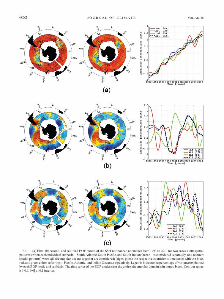
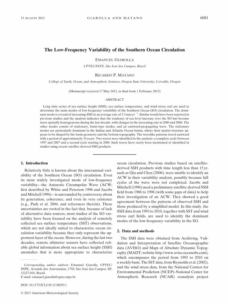
FIG. 1. (a) First, (b) second, and (c) third EOF modes of the SSH normalized anomalies from 1993 to 2010 for two cases: (left; spatial

patterns) when each individual subbasin—South Atlantic, South Pacific, and South Indian Ocean—is considered separately, and (center;

spatial patterns) when all circumpolar oceans together are considered; (right; plots) the respective coefficients time series with the blue,

red, and green colors referring to Pacific, Atlantic, and IndianOceans, respectively. Legends indicate the percentage of variance explained

by each EOFmode and subbasin. The time series of the EOF analysis for the entire circumpolar domain is in dotted black. Contour range

is [-0.6, 0.6] at 0.1 interval.

6082 JOURNAL OF CL IMATE VOLUME 26

(Kalnay et al. 1996), were downloaded from the Inter-

national Research Institute for Climate and Society

(IRI)–Lamont-Doherty Earth Observatory (LDEO)

Climate Data Library (http://iridl.ldeo.columbia.edu/).

To characterize the dominant modes of low-frequency

variability, we calculated the empirical orthogonal

functions (EOFs) of the SSH annual mean anomalies to

discard the seasonal cycles and the 1/48 weekly gridded

data were averaged onto a 18 grid to reduce the influenceof small-scale perturbations. The domain was restricted

to latitudes between 708 and 408S to minimize the in-

fluence of the tropical variability, which is not the scope

of thiswork. Twoapproacheswere used to calculate these

EOFs. The first was to calculate the EOFs of the entire

domain, and the second was to calculate EOFs for each

individual subbasin. There are advantages and disad-

vantages for each approach. The first approach clearly

identifies the dominant mode of variability but obscures

regional variations particularly when—as in this case—

there is a dominant mode of interbasin variability.

Herein, we show the spatial patterns of the entire do-

main and regional EOFs together with the time series of

both calculations. Differences between regional and

circumpolar calculations are discussed within the text.

3. Results

The first EOFmode of SSH variability, which accounts

for approximately 35% of the total variance for all ba-

sins, shows a trend of sea level rise (Fig. 1a). This overall

increasing sea level trend, also captured in the EOF

analysis of separated basins (Fig. 1a, left), has been well

documented in previous studies (e.g., Cabanes et al.

2001; Cazenave and Nerem 2004; Willis et al. 2004;

Lombard et al. 2005; Ishii et al. 2006; Qiu and Chen

2006). The leading causes are the steric expansion, due

to changes in the heat and salt content of the water

column, and the ocean mass redistribution produced by

changes in the ocean circulation (Morrow et al. 2008;

Lombard et al. 2005; Vivier et al. 2005; Roemmich et al.

2007; among others). A third contribution to the sea

level rise could be an increase of the overall mass of the

oceans (Cazenave et al. 2009). The relative contribution

of these effects is uncertain. Previous studies estimated

that steric expansion could explain approximately 50%–

60% of the total sea level rise (e.g., Guinehut et al. 2004;

Lombard et al. 2005). Part of the sea level increase in the

SO is presumably associated with changes of the oceanic

circulation driven by variations of the atmospheric

forcing. Roemmich et al. (2007), for example, posited

that the positive SSH trend over the Pacific is a response

of the oceanic circulation to a strengthening of the wind

stress linked to the southern annular mode (SAM).

The increasing sea level trend, shown in the first EOF

spatial pattern, is in qualitative agreement with the

earlier results reported by, for example, Morrow et al.

(2008) and Lombard et al. (2005), although our calcu-

lation shows a more widespread sea level increase. The

differences can be attributed to the fact thatMorrow et al.

(2008) and Lombard et al. (2005) circumscribed their

analysis to the period 1993–2003 (while we extended the

analysis until 2010) and to the different methodology

used to compute the trends. Tomake amore quantitative

comparison between both estimates, we represented in

Fig. 2a a computation of the SSH linear trend for their

original 1993–2003 period, and in Fig. 2b the time period

was extended until 2010. The comparison indicates that

during the last 7 years there has been an expansion of the

FIG. 2. Trends observed in altimetric SSH (mmyr21) for the

periods (a) 1993–2003 and (b) 1993–2010. The values were esti-

mated through linear regression of monthly anomalies at each 1/48longitude 3 1/48 latitude grid point.


regions with increasing tendencies. In fact, with the ex-

ception of relatively small patches to the southeast of

Africa and in the southern Pacific, most of the SO now

shows an overall sea level increase. The averaged linear

increasing trend, for the SouthernHemisphere oceans at

the latitudinal range considered in Figs. 2a and 2b (708–138S), is about 3.3mmyr21, significant at the 95% con-

fidence level by the Mann–Kendall test. According to

Cazenave et al. (2009), when not only the SO but global

oceans are considered, altimetry-based data indicated

a sea level rise rate of approximately 3.1mmyr21 during

1993–2003 and 2.5mmyr21 over 2003–08. Cazenave

et al. (2009) also report that after 2003 the contribution

of steric expansion has not been preponderant, and since

then the sea level rise of the global oceans has been

caused mainly by land ice contributions. The dominance

of the trend of sea level rise observed in the time series

of the first EOF was confirmed by an ancillary calcula-

tion using detrended data. In this case, all the EOFs

move a rank upward without significant changes in their

spatial or temporal structures. The overall SSH trend

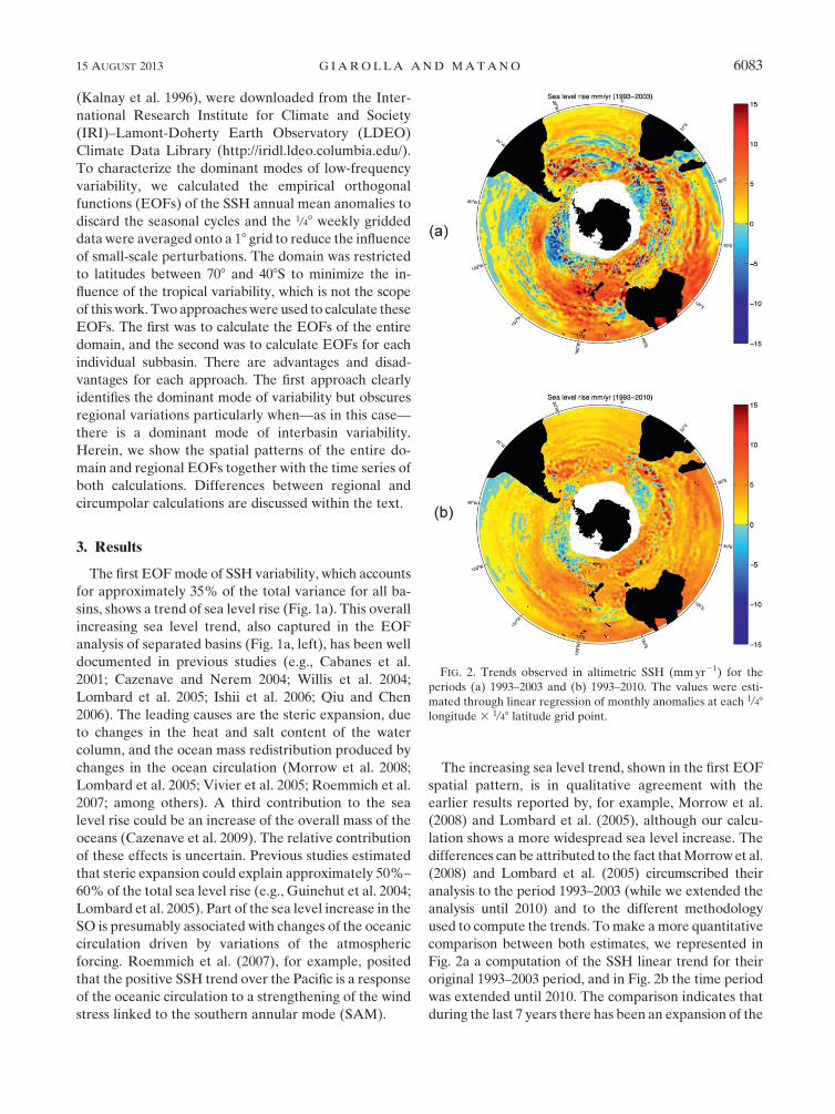
rate on the SO since 1993 has not been linear. Lee and

McPhaden (2008) detected a change of the decadal

tendencies in the SSH of the Indo-Pacific region at the

end of the twentieth century. In Fig. 3a of our study, the

time series of averaged SSH anomalies over the Pacific

region (708–408S, 1508E–708W) shows a trend with an

inflection around the year 2000, in agreement with the

Lee andMcPhaden (2008) study, and a new inflection in

2006, indicating a new change of tendency in the South

Pacific SSH anomalies in this last decade. Analogous

time series calculated for the Indian (278–1228E) and

Atlantic (708W–258E) Oceans, and for all oceans to-

gether (Figs. 3b–d), show comparable inflections of the

FIG. 3. The monthly SSH normalized anomalies with seasonal cycles and averaged between 708 and 408S for (a) Pacific (1508E–708W),

(b) Indian (278–1228E), (c) Atlantic (708W–258E), and (d) all oceans. The black thick curves represent the respective low-pass (3-yr)

filtered values.


trend in 2000 and 2006. Lee and McPhaden (2008) sug-

gest that these changes can be linked to variations in the

strength of subtropical and subpolar gyres. To check

whether similar changes are found in atmospheric fields,

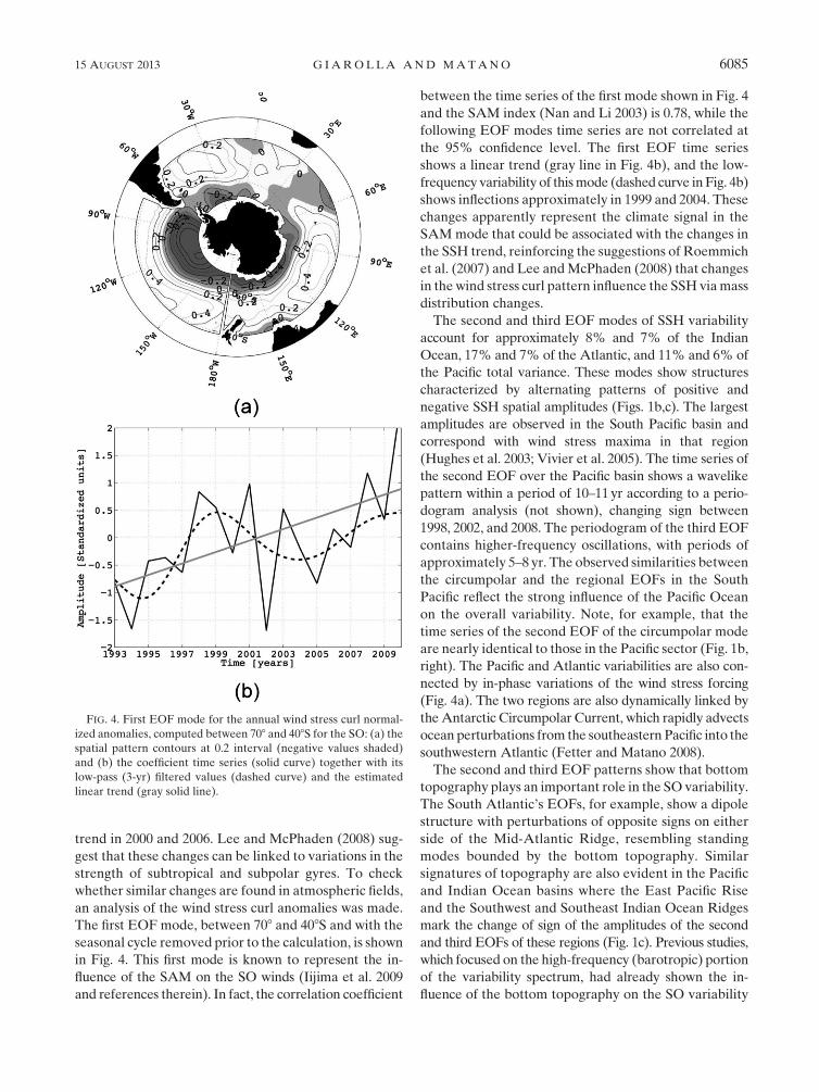
an analysis of the wind stress curl anomalies was made.

The first EOF mode, between 708 and 408S and with the

seasonal cycle removed prior to the calculation, is shown

in Fig. 4. This first mode is known to represent the in-

fluence of the SAM on the SO winds (Iijima et al. 2009

and references therein). In fact, the correlation coefficient

between the time series of the first mode shown in Fig. 4

and the SAM index (Nan and Li 2003) is 0.78, while the

following EOF modes time series are not correlated at

the 95% confidence level. The first EOF time series

shows a linear trend (gray line in Fig. 4b), and the low-

frequency variability of thismode (dashed curve in Fig. 4b)

shows inflections approximately in 1999 and 2004. These

changes apparently represent the climate signal in the

SAMmode that could be associated with the changes in

the SSH trend, reinforcing the suggestions of Roemmich

et al. (2007) and Lee andMcPhaden (2008) that changes

in the wind stress curl pattern influence the SSH viamass

distribution changes.

The second and third EOF modes of SSH variability

account for approximately 8% and 7% of the Indian

Ocean, 17% and 7% of the Atlantic, and 11% and 6% of

the Pacific total variance. These modes show structures

characterized by alternating patterns of positive and

negative SSH spatial amplitudes (Figs. 1b,c). The largest

amplitudes are observed in the South Pacific basin and

correspond with wind stress maxima in that region

(Hughes et al. 2003; Vivier et al. 2005). The time series of

the second EOF over the Pacific basin shows a wavelike

pattern within a period of 10–11yr according to a perio-

dogram analysis (not shown), changing sign between

1998, 2002, and 2008. The periodogram of the third EOF

contains higher-frequency oscillations, with periods of

approximately 5–8 yr. The observed similarities between

the circumpolar and the regional EOFs in the South

Pacific reflect the strong influence of the Pacific Ocean

on the overall variability. Note, for example, that the

time series of the second EOF of the circumpolar mode

are nearly identical to those in the Pacific sector (Fig. 1b,

right). The Pacific and Atlantic variabilities are also con-

nected by in-phase variations of the wind stress forcing

(Fig. 4a). The two regions are also dynamically linked by

theAntarctic Circumpolar Current, which rapidly advects

ocean perturbations from the southeastern Pacific into the

southwestern Atlantic (Fetter and Matano 2008).

The second and third EOF patterns show that bottom

topography plays an important role in the SO variability.

The South Atlantic’s EOFs, for example, show a dipole

structure with perturbations of opposite signs on either

side of the Mid-Atlantic Ridge, resembling standing

modes bounded by the bottom topography. Similar

signatures of topography are also evident in the Pacific

and Indian Ocean basins where the East Pacific Rise

and the Southwest and Southeast Indian Ocean Ridges

mark the change of sign of the amplitudes of the second

and third EOFs of these regions (Fig. 1c). Previous studies,

which focused on the high-frequency (barotropic) portion

of the variability spectrum, had already shown the in-

fluence of the bottom topography on the SO variability

FIG. 4. First EOF mode for the annual wind stress curl normal-

ized anomalies, computed between 708 and 408S for the SO: (a) the

spatial pattern contours at 0.2 interval (negative values shaded)

and (b) the coefficient time series (solid curve) together with its

low-pass (3-yr) filtered values (dashed curve) and the estimated

linear trend (gray solid line).


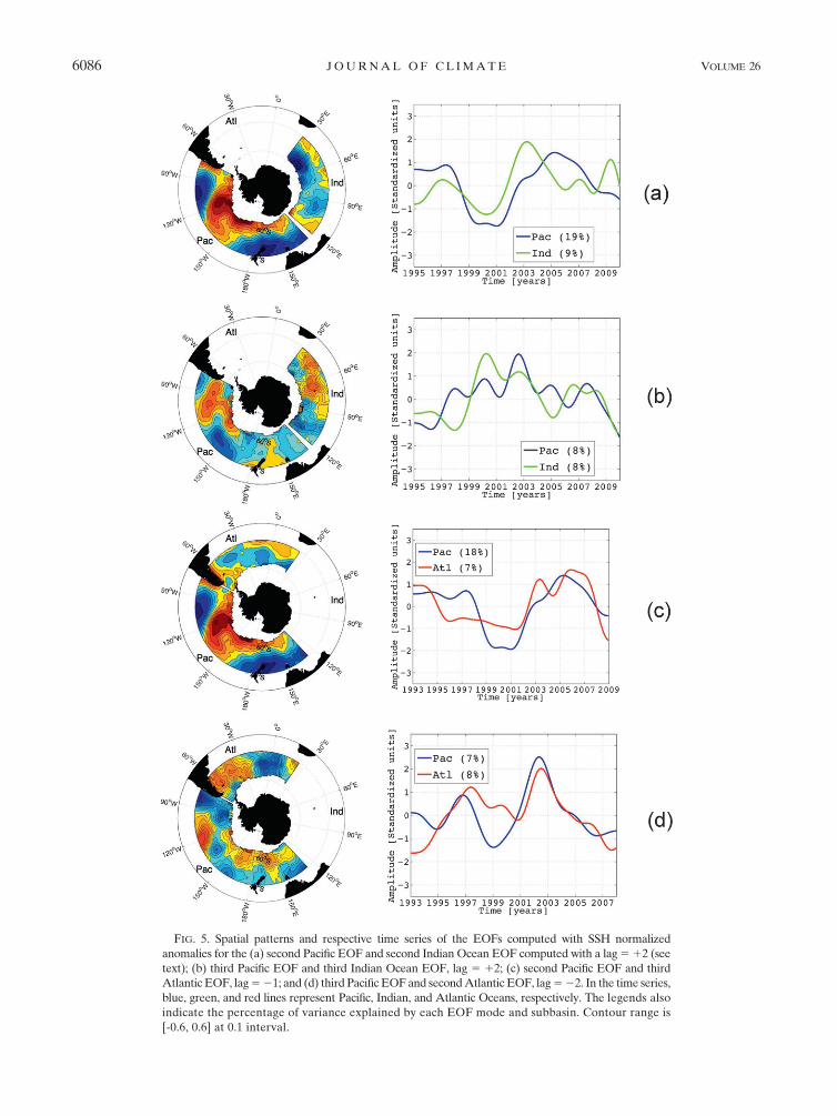
FIG. 5. Spatial patterns and respective time series of the EOFs computed with SSH normalized

anomalies for the (a) second Pacific EOF and second Indian Ocean EOF computed with a lag512 (see

text); (b) third Pacific EOF and third Indian Ocean EOF, lag 5 12; (c) second Pacific EOF and third

Atlantic EOF, lag521; and (d) third PacificEOF and secondAtlantic EOF, lag522. In the time series,

blue, green, and red lines represent Pacific, Indian, and Atlantic Oceans, respectively. The legends also

indicate the percentage of variance explained by each EOF mode and subbasin. Contour range is

[-0.6, 0.6] at 0.1 interval.


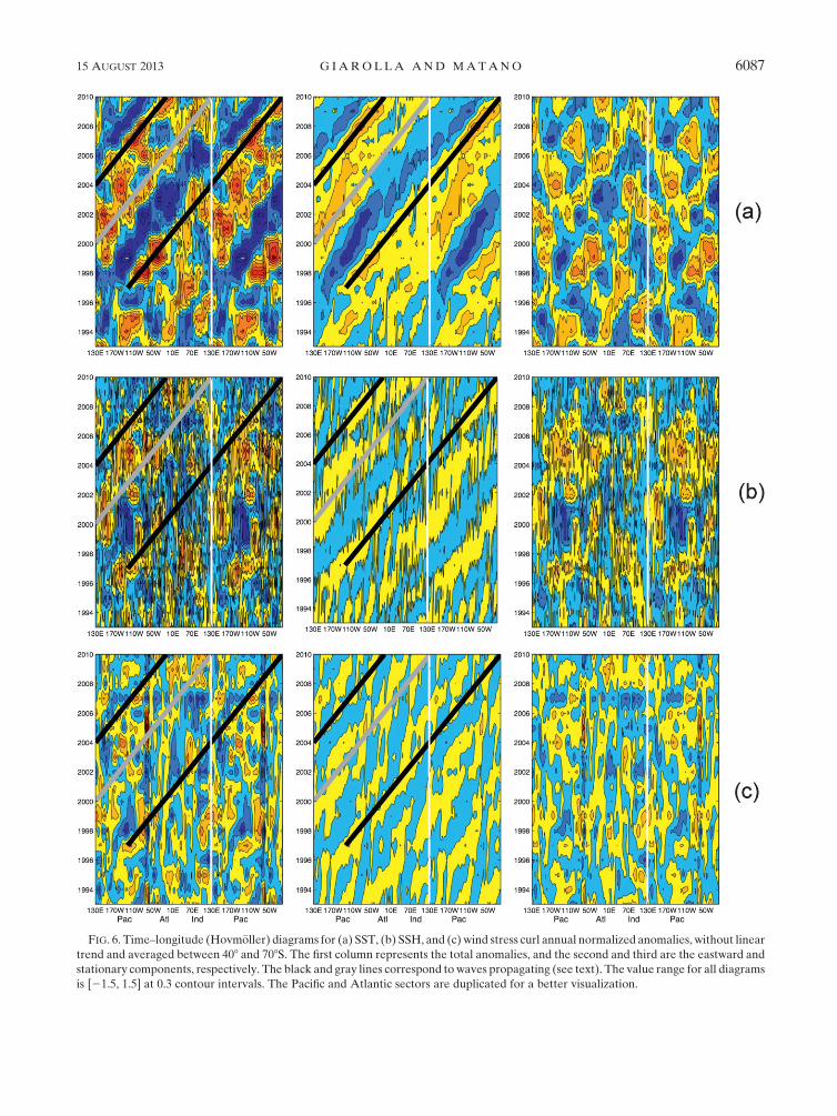
FIG. 6. Time–longitude (Hovm€oller) diagrams for (a) SST, (b) SSH, and (c) wind stress curl annual normalized anomalies, without linear

trend and averaged between 408 and 708S. The first column represents the total anomalies, and the second and third are the eastward and

stationary components, respectively. The black and gray lines correspond to waves propagating (see text). The value range for all diagrams

is [21.5, 1.5] at 0.3 contour intervals. The Pacific and Atlantic sectors are duplicated for a better visualization.


(Hughes et al. 2003; Weijer and Gille 2005). Our analysis

indicates that similar modes are also evident in the low-

frequency portion of the spectrum. We surmise that the

observed variations represent low-frequency modula-

tions of topographically trapped modes. Such modula-

tion has already been documented in the Argentinean

basin (Saraceno et al. 2004).

The variability patterns described above are charac-

terized by a circumpolar structure of highs and lows with

regional variations. The wavelike structure of this pat-

tern is emphasized by the near quadrature of the time

series of the second and third EOFs of the circumpolar

calculation, which is symptomatic of propagating phe-

nomena (Figs. 1b,c). The regional EOFs were also

computed with 1 or 2 years removed prior to calcula-

tions, at the beginning or the end of the data, to be in-

tercompared with lags in time. The lagged correlation of

the time series of the regional modes is further evidence

of a propagating phenomenon. For example, the corre-

lation between the second mode of the Indian Ocean

sector and the secondmode of the Pacific sector increases

from 0.0 to 0.48 with a time lag of 12 for the Indian

Ocean sector (i.e., events from the IndianOcean precede

by 2 years those in the Pacific Ocean; Fig. 5a). The cor-

relation between the third mode of the Indian Ocean and

the third mode of the Pacific increases from 0.21 to 0.61

(also with a time lag of12; Fig. 5b). The time series of the

Pacific and Atlantic are similarly correlated. The second

mode of the Pacific and the third mode of the Atlantic

have a correlation of 0.68 with a time lag of21, while the

third mode of the Pacific has a correlation of 0.62 with the

second mode of the Atlantic with a time lag of 22 (Figs.

5c,d). Thus, the significant correlations betweenmodes at

1–2-yr time lags indicate that these modes might represent

the same phenomenon, differing only by a phase shift.

To further investigate the propagating nature of the

patterns described above, we constructed Hovm€oller

diagrams of detrended SSH, SST, and wind stress curl

annual anomalies for the latitudinal band between 408and 708S (Fig. 6, first column). At least two circumpolar

waves can be identified in those diagrams, although it is

not straightforward to separate them because (as seen in

Fig. 6) anomalies of a propagating wave can possibly

merge with those of another new wave being generated.

Despite this, we defined one wave starting in the east

Pacific region, and propagating from 1997 to 2010 and

probably beyond (black thick lines, Fig. 6) and a second

wave from 2001 to 2010 (gray lines, Fig. 6). The first

wave completes a cycle around the globe in approxi-

mately 10 years. For the first wave, the anomalies are

most intense in the Pacific and Atlantic sectors (1108W–

108E). The propagating patterns are similar to those

ascribed to the ACW. The signal is more clearly defined

in the SST than in the SSH and the wind stress curl data.

To quantify the contribution of the eastward-propagating

signal to the variability of each of these variables we

separated the eastward-propagating component from

the stationary component using the method described

by Park et al. (2004), where longitude–time variations

of SST, SSH, and wind stress curl are represented as

a sum of Fourier harmonics composed of westward- and

eastward-propagating waves and standing waves are

defined as the sum of two waves of equal amplitude

propagating in opposite directions. These components

are shown in Fig. 6, second and third columns. The re-

sults show a clear eastward-propagating signal in the

SST, SSH, and wind stress curl fields, especially in the

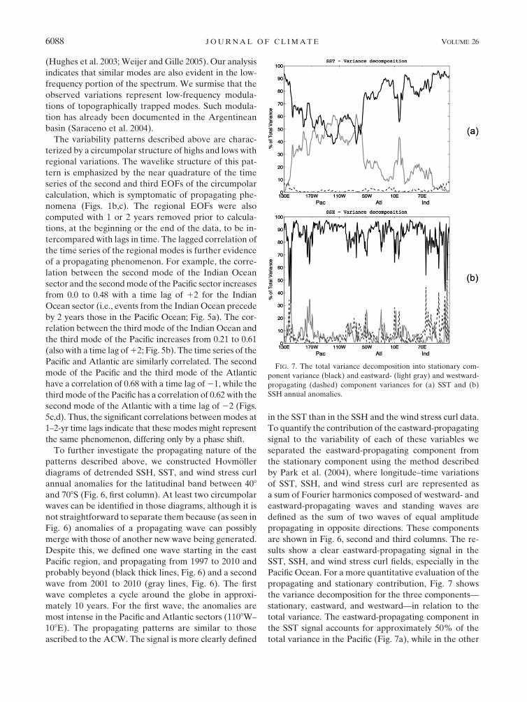
Pacific Ocean. For a more quantitative evaluation of the

propagating and stationary contribution, Fig. 7 shows

the variance decomposition for the three components—

stationary, eastward, and westward—in relation to the

total variance. The eastward-propagating component in

the SST signal accounts for approximately 50% of the

total variance in the Pacific (Fig. 7a), while in the other

FIG. 7. The total variance decomposition into stationary com-

ponent variance (black) and eastward- (light gray) and westward-

propagating (dashed) component variances for (a) SST and (b)

SSH annual anomalies.


basins the stationary component accounts for a higher

amount of the total variance. The eastward-propagating

component of the total variance of the SSH signal

(Fig. 7b), and of the wind stress curl signal (not shown),

are substantially smaller than their stationary compo-

nents for all the basins. The westward component of the

SST variance is negligible (e.g., Park et al. 2004), but the

westward component of the SSH, which represents

Rossby waves (e.g., Qiu and Chen 2006), is not negligi-

ble. The larger contribution of the eastward-propagating

component to the SST variability indicates that this signal

is largely confined to the upper layers of the ocean. The

SSH anomalies, which are more influenced than the SST

anomalies by variability in the deeper layers, do not show

such a dominant contribution. In addition, the relation

between SSH and SST is particularly difficult to esta-

blish in the ACW because it involves a coupled ocean–

atmosphere phenomenon (see, e.g., Venegas 2003 and

references therein). SSTs are essentially advected by the

geostrophic currents generated by the SSH gradients, but

SSTs are not a passive tracer since they influence the

overlying atmosphere and, hence, the wind stress distri-

bution that forces the SSHs.

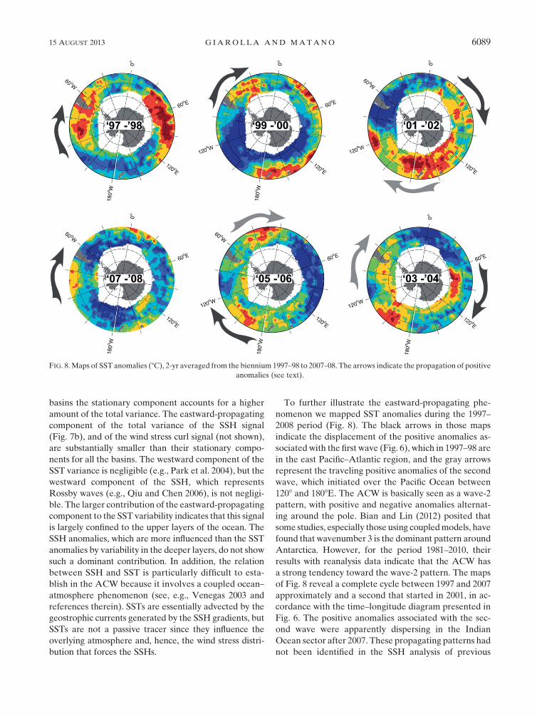
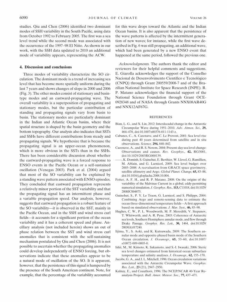
To further illustrate the eastward-propagating phe-

nomenon we mapped SST anomalies during the 1997–

2008 period (Fig. 8). The black arrows in those maps

indicate the displacement of the positive anomalies as-

sociated with the first wave (Fig. 6), which in 1997–98 are

in the east Pacific–Atlantic region, and the gray arrows

represent the traveling positive anomalies of the second

wave, which initiated over the Pacific Ocean between

1208 and 1808E. The ACW is basically seen as a wave-2

pattern, with positive and negative anomalies alternat-

ing around the pole. Bian and Lin (2012) posited that

some studies, especially those using coupledmodels, have

found that wavenumber 3 is the dominant pattern around

Antarctica. However, for the period 1981–2010, their

results with reanalysis data indicate that the ACW has

a strong tendency toward the wave-2 pattern. The maps

of Fig. 8 reveal a complete cycle between 1997 and 2007

approximately and a second that started in 2001, in ac-

cordance with the time–longitude diagram presented in

Fig. 6. The positive anomalies associated with the sec-

ond wave were apparently dispersing in the Indian

Ocean sector after 2007. These propagating patterns had

not been identified in the SSH analysis of previous

FIG. 8. Maps of SST anomalies (8C), 2-yr averaged from the biennium 1997–98 to 2007–08. The arrows indicate the propagation of positive

anomalies (see text).


studies. Qiu and Chen (2006) identified two dominant

modes of SSH variability in the South Pacific, using data

from October 1992 to February 2005. The first was a sea

level trend while the second mode was associated with

the occurrence of the 1997–98 El Ni~no. As shown in our

work, with the SSH data updated to 2010 an additional

mode of variability appears, representing the ACW.

4. Discussion and conclusions

Three modes of variability characterize the SO cir-

culation. The dominant mode is a trend of increasing sea

level that has become more spatially uniform during the

last 7 years and shows changes of slope in 2000 and 2006

(Fig. 3). The othermodes consist of stationary and basin-

type modes and an eastward-propagating wave. The

overall variability is a superposition of propagating and

stationary modes, but the particular contribution of

standing and propagating signals vary from basin to

basin. The stationary modes are particularly dominant

in the Indian and Atlantic Ocean basins, where their

spatial structure is shaped by the basin geometry and the

bottom topography. Our analysis also indicates that SSTs

and SSHs have different contributions from steady and

propagating signals. We hypothesize that is because the

propagating signal is an upper-ocean phenomenon,

which is more obvious in the SSTs than in the SSHs.

There has been considerable discussion about whether

the eastward-propagating wave is a forced response to

ENSO events in the Pacific Ocean or a self-sustained

oscillation (Venegas 2003). Park et al. (2004) argued

that most of the SO variability can be explained by

a standing wave pattern associated with ENSO episodes.

They concluded that eastward propagation represents

a relatively minor portion of the SST variability and that

the propagating signal has an intermittent phase and

a variable propagation speed. Our analysis, however,

suggests that eastward propagation is a robust feature of

the SO variability—it is observed in the SST, mainly in

the Pacific Ocean, and in the SSH and wind stress curl

fields—it accounts for a significant portion of the ocean

variability and it has a coherent speed and phase. An-

cillary analysis (not included herein) shows an out of

phase relation between the SST and wind stress curl

anomalies that is consistent with the self-sustaining

mechanism postulated by Qiu and Chen (2006). It is not

possible to ascertain whether the propagating anomalies

could develop independently of ENSO forcing, but ob-

servations indicate that these anomalies appear to be

a natural mode of oscillation of the SO. It is apparent,

however, that the persistence of this signal is hampered by

the presence of the South American continent. Note, for

example, that the percentage of the variability accounted

for this wave drops toward the Atlantic and the Indian

Ocean basins. It is also apparent that the persistence of

the wave patterns is affected by the intermittent genera-

tion of new waves; for instance, while the first wave de-

scribed in Fig. 6 was still propagating, an additional wave,

which had been generated by a new ENSO event that

happened at the same period, followed the previous one.

Acknowledgments. The authors thank the editor and

reviewers for their helpful comments and suggestions.

E. Giarolla acknowledges the support of the Conselho

Nacional de Desenvolvimento Cient�ıfico e Tecnol�ogico

(CNPQ) through Grant 200559/2008-7 and of the Bra-

zilian National Institute for Space Research (INPE). R.

P. Matano acknowledges the financial support of the

National Science Foundation through Grant OCE-

0928348 and of NASA through Grants NNX08AR40G

and NNX12AF67G.

REFERENCES

Bian, L. G., and X. Lin, 2012: Interdecadal change in the Antarctic

Circumpolar Wave during 1951–2010. Adv. Atmos. Sci., 29,

464–470, doi:10.1007/s00376-011-1143-z.

Cabanes, C., A. Cazenave, and C. Le Provost, 2001: Sea level rise

during past 40 years determined from satellite and in situ

observations. Science, 294, 840–842.

Cazenave, A., andR. S. Nerem, 2004: Present-day sea level change:

Observations and causes. Rev. Geophys., 42, RG3001,

doi:10.1029/2003RG000139.

——,K.Dominh, S.Guinehut, E. Berthier,W. Llovel, G. Ramillien,

M. Ablain, and G. Larnicol, 2009: Sea level budget over

2003–2008: A reevaluation from GRACE space gravimetry,

satellite altimetry and Argo.Global Planet. Change, 65, 83–88,

doi:10.1016/j.gloplacha.2008.10.004.

Fetter, A. F. H., and R. P. Matano, 2008: On the origins of the

variability of the Malvinas Current in a global, eddy-permitting

numerical simulation. J.Geophys. Res., 113,C11018, doi:10.1029/

2008JC004875.

Guinehut, S., P. Y. Le Traon, G. Larnicol, and S. Philipps, 2004:

Combining Argo and remote-sensing data to estimate the

ocean three-dimensional temperature fields—Afirst approach

based on simulated observations. J. Mar. Syst., 46, 85–98.Hughes, C. W., P. L. Woodworth, M. P. Meredith, V. Stepanov,

T. Whitworth, and A. R. Pyne, 2003: Coherence of Antarctic

sea levels, SouthernHemisphere annularmode, and flow through

Drake Passage. Geophys. Res. Lett., 30, 1464, doi:10.1029/

2003GL017240.

Iijima, Y., S. Aoki, and K. Kutsuwada, 2009: The Southern an-

nular mode and opposite-phased basin mode of the Southern

Ocean circulation. J. Oceanogr., 65, 53–60, doi:10.1007/

s10872-009-0005-0.

Ishii, M., M. Kimoto, K. Sakamoto, and S.-I. Iwasaki, 2006: Steric

sea level changes estimated from historical ocean subsurface

temperature and salinity analyses. J. Oceanogr., 62, 155–170.

Jacobs, G. A., and J. L.Mitchell, 1996: Ocean circulation variations

associated with the Antarctic Circumpolar Wave. Geophys.

Res. Lett., 23 (21), 2947–2950.

Kalnay, E., and Coauthors, 1996: The NCEP/NCAR 40-Year Re-

analysis Project. Bull. Amer. Meteor. Soc., 77, 437–471.


Lee, T., andM. J. McPhaden, 2008: Decadal phase change in large-

scale sea level and winds in the Indo-Pacific region at the end

of the 20th century.Geophys. Res. Lett., 35, L01605, doi:10.1029/

2007GL032419.

Lombard, A., A. Cazenave, P. Y. Le Traon, and M. Ishii, 2005:

Contribution of thermal expansion to present-day sea level

change revisited. Global Planet. Change, 47, 1–16.

Morrow, R., G. Valladeau, and J.-B. Sallee, 2008: Observed sub-

surface signature of Southern Ocean sea level rise. Prog.

Oceanogr., 77, 351–366.

Nan, S., and J. Li, 2003: The relationship between summer pre-

cipitation in the Yangtze River valley and the boreal spring

Southern Hemisphere annular mode. Geophys. Res. Lett., 30,

2266, doi:10.1029/2003GL018381.

Park, Y.-H., F. Roquet, and F. Vivier, 2004: Quasi-stationary ENSO

wave signals versus the Antarctic Circumpolar Wave scenario.

Geophys. Res. Lett., 31, L09315, doi:10.1029/2004GL019806.

Qiu, B., and S. Chen, 2006: Decadal variability in the large-scale

sea surface height field of the South Pacific Ocean: Observa-

tions and causes. J. Phys. Oceanogr., 36, 1751–1762.

Reynolds, R. W., N. A. Rayner, T. M. Smith, D. C. Stokes, and

W.Wang, 2002: An improved in situ and satellite SST analysis

for climate. J. Climate, 15, 1609–1625.

Roemmich, D., J. Gilson, R. Davis, P. Sutton, S. Wijffels, and

S. Riser, 2007: Decadal spinup of the South Pacific subtropical

gyre. J. Phys. Oceanogr., 37, 162–173.

Saraceno, M., C. Provost, A. R. Piola, J. Bava, and A. Gagliardini,

2004: Brazil Malvinas frontal system as seen from 9 years of

advanced very high resolution radiometer data. J. Geophys.

Res., 109, C05027, doi:10.1029/2003JC002127.

Venegas, S. A., 2003: The Antarctic Circumpolar Wave: A com-

bination of two signals? J. Climate, 16, 2509–2525.

Vivier, F., K. A. Kelly, and M. Harismendy, 2005: Causes of large-

scale sea level variations in the Southern Ocean: Analysis of

sea level and a barotropic model. J. Geophys. Res., 110,C09014, doi:10.1029/2004JC002773.

Weijer, W., and S. T. Gille, 2005: Adjustment of the Southern

Ocean to wind forcing on synoptic time scales. J. Phys. Oce-

anogr., 35, 2076–2089.

White, W. B., and R. G. Peterson, 1996: AnAntarctic Circumpolar

Wave in surface pressure, wind, temperature and sea-ice ex-

tent. Nature, 380, 699–702.Willis, J. K., D. Roemmich, and B. Cornuelle, 2004: Interannual

variability in upper ocean heat content, temperature, and

thermosteric expansion on global scales. J. Geophys. Res., 109,

C12036, doi:10.1029/2003JC002260.


the low-frequency variability of the southern …klinck/reprints/pdf/giarollajclim2013.pdfthe...

Documents