The Lightbulb Paradox: Using Behavioral Economics for Policy

Evaluation

Hunt Allcott and Dmitry Taubinsky�

July 16, 2013

Abstract

In an e¤ort to reduce energy use, governments in the United States and many other coun-

tries subsidize energy e¢ cient lightbulbs or ban traditional incandescent bulbs. We evaluate

one important rationale for these policies: that imperfect information or attentional biases

cause consumers to purchase more incandescents than they would in their private optima. We

formalize a model of consumer choice that allows for such biases and develop formulas that

allow optimal policy to be approximated using su¢ cient statistics from simple randomized con-

trol trials (RCTs). We then present results from two RCTs that provide information about and

draw attention to the energy costs of di¤erent lightbulbs. The treatment e¤ects could provide

support for subsidies on the order of those currently in place in parts of the U.S. However, there

is no evidence to suggest that a ban on traditional incandescent lightbulbs increases welfare.

JEL Codes: D03, D12, H21, H31, L94, Q41, Q48.Keywords: Behavioral public economics, energy e¢ ciency, �eld experiments, internality

taxes, lightbulbs, optimal policy, Time-Sharing Experiments for the Social Sciences.

� � � � � � � � � � � � � � � � � � � � � � � � � � � �

We are grateful to colleagues and seminar audiences for helpful feedback. We thank our

research sta¤ - Jeremiah Hair, Nina Yang, and Ti¤any Yee - as well as management at the

partner company, for their work on the in-store �eld experiment. Thanks to Stefan Subias,

Benjamin DiPaola, and Poom Nukulkij at GfK for their work on the TESS �eld experiment.

We are grateful to the National Science Foundation and the Sloan Foundation for �nancial

support.

�Allcott: New York University and NBER. Taubinsky: Harvard University.

1

1 Introduction

Compared to standard incandescents, compact �uorescent lightbulbs (CFLs) typically last eight

times longer and use four times less electricity. Although CFLs cost several dollars to purchase,

compared to a dollar or less for incandescents, using a CFL saves about $5 each year once the costs

of electricity and replacement bulbs are included. Despite this cost advantage, only 28 percent of

residential sockets that could hold CFLs in 2010 actually had them (DOE 2010). In that year,

using incandescents instead of CFLs cost US households $15 billion dollars.1

Lightbulbs are a canonical example of the Energy Paradox (Ja¤e and Stavins 1994): the low

adoption of energy e¢ cient technologies despite potentially large savings. This "Lightbulb Paradox"

has inspired policymakers to take action. Regulated and government-run electric utilities spent $252

million subsidizing and otherwise promoting CFLs in 2010 (DOE 2010). Furthermore, the Energy

Independence and Security Act of 2007 sets minimum e¢ ciency standards that ban traditional

incandescent lightbulbs between 2012 and 2014 and are likely to require e¢ ciency at least as

good as CFLs by 2020. The lighting e¢ ciency standards have generated vigorous debate, with

advocates pointing out that consumers will enjoy large energy cost savings (NRDC 2011) and

opponents suggesting that they are "an example of over-reaching government intrusion into our

lives" (Formisano 2008). Meanwhile, Argentina, Australia, Brazil, Canada, China, Cuba, the

European Union, Israel, Malaysia, Russia, and Switzerland have banned some or all incandescent

light bulbs.

Governments often subsidize or mandate goods and tax or ban bads. One economic reason for

such intervention is externalities. In the case of lightbulbs, one might argue that electricity prices are

below social cost due to unpriced externalities from carbon dioxide, and banning energy ine¢ cient

lightbulbs is a welfare-improving second best policy in the absence of a price on carbon emissions.

However, unless the marginal damages from carbon dioxide are much larger than the standard

U.S. Government estimates (Interagency Working Group 2013), the marginal cost of residential

electricity in most of the United States is above social cost because retailers typically include much

of �xed distribution costs in marginal prices.2 Furthermore, lightbulbs are more frequently used at

night, when real-time wholesale electricity prices are low relative to the time-invariant prices that

nearly all residential consumers pay. This suggests that if the primary distortion were mispriced

residential electricity, it might actually be optimal to subsidize incandescents.

A second potential reason for intervention is to protect consumers who may be imperfectly

informed or may not act in their own best interests, as is sometimes argued in cases like addictive

drugs, seat belts, and �nancial products like high-interest loans. In the case of lightbulbs, people

1Throughout the paper, we assume that incandescents and CFLs last an average of 1000 and 8000 hours, respec-tively. (To receive the Energy Star rating, a CFL must last a median of 8000 hours in tests.) The national averageelectricity price is $0.10 per kilowatt-hour. Our cost estimate of $15 billion is equal to 5.8 billion residential sockets(DOE 2012), times the 80 percent of sockets that can accommodate CFLs (DOE 2010) minus the actual "socketshare" of 28 percent (DOE 2010), times $5 per socket per year.

2See Davis and Muehlegger (2010) for a discussion of this for retail natural gas prices.

2

may not know how much electricity an incandescent uses, or they may be inattentive to this

additional cost, like consumers in Gabaix and Laibson (2006) or Chetty, Looney, and Kroft (2009).

Extending a term from Herrnstein et al. (1993), we call this the "internality rationale" for energy

e¢ ciency policy. This rationale has been suggested by energy e¢ ciency specialists (Nadel 2011),

government regulatory impact analyses (NHTSA 2010), and academic analyses (Parry, Evans, and

Oates 2010).3 If lightbulb buyers are well-informed utility maximizers, however, our "Lightbulb

Paradox" might not be much of a paradox: the market share of CFLs could be so low simply

because many consumers don�t like some of their attributes. In this case, one would need to point

to some third market failure to argue that subsidies for CFLs or bans on incandescents could

increase welfare.4

This paper tests one aspect of the internality rationale: whether informational or attentional

biases can justify lightbulb subsidies and bans. We begin by formalizing a theoretical framework

in which consumers make a discrete choice, which in the empirical application will be between an

incandescent and a CFL. Some consumers may misjudge the true di¤erence in utility they would

experience from each product, and we label the dollar value of this potential mistake the "inter-

nality." The internality is directly analogous to an externality: it is a wedge between willingness

to pay and social welfare, and it may be heterogeneous across consumers. Just the optimal exter-

nality tax equals the average marginal externality (Diamond 1973), the optimal internality tax (in

our example, a CFL subsidy) equals the average marginal internality. The welfare e¤ect of a ban

depends on the true utility experienced by the set of consumers who would buy incandescents in

the absence of the ban.

We then present the results of two randomized control trials (RCTs) designed to debias con-

sumers. The �rst is a "framed �eld experiment" (Levitt and List 2009) with a large home improve-

ment retailer. Our sta¤ intercepted shoppers, used an iPad to deliver information about energy

costs and bulb lifetimes to the treatment group, and then gave coupons with randomly assigned

CFL subsidies. While a 20 percent subsidy increased CFL market share by about 10 percentage

points, the informational intervention had statistically zero e¤ect.

The second RCT is an "artefactual �eld experiment" (Levitt and List 2009) using Time-Sharing

Experiments for the Social Sciences (TESS). TESS is a high-quality "nationally-representative" on-

line survey platform that has also been used by Allcott (2013), Fong and Luttmer (2009), Heiss,

McFadden, and Winter (2007), Newell and Siikamaki (2013), Rabin and Weizsacker (2009), and

many others. We gave consumers a shopping budget and asked them to make a series of choices

3Nadel (2011) argues that one market failure addressed by energy e¢ ciency standards is "rush purchases when anexisting appliance breaks down." The o¢ cial Regulatory Impact Analysis for the increase in the Corporate AverageFuel Economy standard for 2012 to 2016 (NHTSA 2010) argues that even without counting the externality reductions,the regulation would increase consumer welfare, perhaps because consumers have incorrect perceptions of the valueof fuel economy. Parry, Evans, and Oates (2010) analyze whether energy e¢ ciency standards are welfare improving.They study two market failures that could justify such regulation: externalities and what they call "misperceptionsmarket failures."

4Other market failures might include agency problems in real estate markets (colloquially called the "landlord-tenant" problem) or uninternalized R&D spillovers for developers of energy e¢ cient lighting technologies.

3

between CFLs and incandescents at di¤erent relative prices. The experiment was incentive com-

patible: one of the choices was randomly selected to be the consumer�s "o¢ cial purchase," and the

consumer received those lightbulbs and kept the remainder of his or her shopping budget. We then

gave the treatment group information about lightbulb energy costs and lifetimes. After this infor-

mational intervention, we again asked all consumers to choose between CFLs and incandescents.

The informational intervention increased average willingness to pay for CFLs by $1.12.

For each experiment, we extend the analysis by mapping empirical results into optimal poli-

cies. To do this, we make a key assumption: the treatment e¤ect of information identi�es the

magnitude of the bias. In other words, we assume that the informational interventions act only by

fully informing or debiasing consumers subject to imperfect information or inattention. In both

experiments, we will need to document the extent to which consumers internalized and understood

the information as well as consider external validity and potential experimenter demand e¤ects.

Although we took a series of steps to deal with these issues ex ante and to document them ex post,

such concerns are important. Furthermore, informational interventions do not provide evidence on

whether present bias or other biases could justify subsidies and bans.5

The in-store experiment was designed to identify the slope of demand and the e¤ect of the

bias on demand. We derive a formula that shows how these two quantities are su¢ cient statistics

for an approximation to the optimal subsidy. Intuitively, the formula shows that the average

marginal internality is the price change that would have the same e¤ect on demand as the debiasing

intervention. Given that the intervention had no statistical e¤ect, we cannot reject that the optimal

subsidy is zero. Our formula bounds the optimal subsidy for a 60-Watt equivalent CFL between

negative 30 cents and positive 35 cents per CFL with 90 percent con�dence.

The design of the TESS experiment allows us to go much further than with the in-store ex-

periment, because it identi�es the joint distribution of relative valuations of CFLs in consumers�

baseline (potentially biased) state and their unbiased state. Using the bias estimated at each point

on the demand curve, we maximize welfare over all possible values of the subsidy. The results

suggest that the optimal subsidy is between $1 and $2. For comparison, CFL subsidies o¤ered by

utilities are often in the range of $1 to $2 per bulb. We also observe a large set of consumers who

purchase incandescents at baseline and are still willing to pay substantially more for incandescents

after the informational intervention. This implies that given a choice set of incandescents and

CFLs, the welfare losses from banning incandescents would be large.6

Our major contribution is that we show how to use the tools of public economics in conjunction

with psychologically-motivated randomized experiments to evaluate an important public policy.

5 In the TESS experiment, however, we show that present bias revealed on hypothetical intertemporal choicequestions is not correlated with willingness to pay for CFLs, which we view as initial suggestive evidence that presentbias does not play a large role either.

6To be clear, the U.S. lighting e¢ ciency standards do not require CFLs. Although CFLs are currently themost commonly-sold lighting technology that meets the standard, advanced incandescents and light-emitting diodes(LEDs) also comply. This highlights that our analysis models a discrete choice between incandescents and CFLs,while technological change will change the choice set over time.

4

Although our �eld experiments focus on only one product, our framework connects to several

broader literatures at the intersection of behavioral and public economics. Related theoretical

papers include Bernheim and Rangel (2004), Gul and Pesendorfer (2007), and O�Donoghue and

Rabin (2006), who study taxes when consumers are present biased or otherwise make mistakes.

There are also several papers that study energy taxes, energy e¢ ciency standards, or subsidies

for energy e¢ cient goods in the presence of biased consumers, including Allcott, Mullainathan,

and Taubinsky (2013), Heutel (2011), and Parry Evans, and Oates (2010). Our paper stands out

relative to these theoretical analyses because we also use �eld experiments to calibrate policies and

welfare e¤ects. This idea that �eld experiments can identify the magnitude of biases is inspired by

Chetty, Looney, and Kroft (2009), who estimate the magnitude of inattention to sales taxes using the

treatment e¤ect of an intervention that posted tax-inclusive purchase prices. One important feature

of this approach is that it "respects choice" in the sense of Bernheim and Rangel (2009): instead of

imposing external assumptions on decisionmakers�true utility, we conduct welfare analysis using

their own choices in a "debiased" state.

Our experiments are also related to studies of the e¤ects of information disclosure on consumer

choice in various domains, including Choi, Laibson, and Madrian (2010) and Duarte and Hastings

(2012) on �nancial choices, Greenstone, Oyer, and Vissing-Jorgensen (2006) on securities, Bhargava

and Manoli (2013) on takeup of social programs, Jin and Sorensen (2006), Kling et al. (2012), and

Scanlon et al. (2002) on health insurance plans, Pope (2009) on hospitals, Bollinger, Leslie,and

Sorensen (2011) on nutrition, Figlio and Lucas (2004) and Hastings and Weinstein (2008) on school

choice, and many others. Houde (2012) is conceptually related: he uses quasi-experimental variation

with a structural demand model to estimate how the Energy Star label a¤ects consumer welfare.

To our knowledge, however, this is the �rst RCT used to study the e¤ects of energy use information

on durable good purchases, although papers such as Newell and Siikamaki (2013) and Ward, Clark,

Jensen, Yen, and Russell (2011) study e¤ects on stated preferences using hypothetical choices.

Section 2 lays out our theoretical framework and derives optimal policies and welfare e¤ects.

Sections 3 and 4 present the in-store and TESS experiments, respectively. Section 5 concludes.

2 Theoretical Framework

2.1 Consumers

We model consumers that make one of two choices, labeled E and I. In our empirical application,

E represents the purchase of an energy e¢ cient product (the CFL), while I is an energy ine¢ -

cient product (the incandescent). More generally, this model could capture any choice over which

consumers might misoptimize.

Products j 2 fE; Ig are sold at prices pj , and p = pE � pI is the relative price of E. Wede�ne vj as the consumer�s true utility from consuming product j, and we call v = vE � vI the

5

relative true utility from E. In our empirical application, v could be determined by any and all of

the di¤erences between CFLs and incandescents, such as electricity costs, longer lifetime, mercury

content, brightness, and "warm glow" utility from reduced environmental impact.

A fully optimizing consumer chooses E if and only if v > p. A misoptimizing consumer chooses

E if and only if v � b(p) > p, where b(p) is a bias that may depend on p and is continuously

di¤erentiable in p. To simplify notation, we will typically denote bias by b rather than b(p). The

pair (v; b), which we will refer to as a consumer�s "type," is jointly distributed according to a

distribution F . We denote the conditional distribution of v given b by Fvjb(�jb). We assume thatfor each b, the distribution Fvjb(�jb) has an atomless and continuous density function fvjb(�jb). Forsimplicity, we will also assume that b takes on �nitely many values, though the analysis easily

generalizes. We let q(b) denote the fraction of consumers with bias b.

We also call b the "internality," to highlight the analogy to externalities. While an externality

is a wedge between private willingness-to-pay (WTP) and social welfare, the internality is a wedge

between private WTP and true private welfare. This is a reduced form representation of many

biases that could cause consumers not to maximize experienced utility, including misperceptions

of any product attribute. It allows for dependencies between bias b, true valuation v, and price p,

as theories of endogenous inattention would imply. In our empirical application, we think of the

bias as arising from consumers�undervaluation of energy costs due to a set of informational and

attentional biases that we discuss later.

This model of discrete choice generates continuous demand curves for product E. Let DR(p) =

1 � F (p) denote the �unbiased� demand curve for E, let Db(p) = q(b)[1 � Fvjb(p + bjb)] denotethe demand curve of consumers with bias b, let DRb = q(b)[1� Fvjb(pjb)] denote what would be thedemand curve of consumers with bias b if they were �debiased,�and let D(p) =

PDb(p) denote the

total demand curve of all consumers. Our assumptions about b and F imply that all demand curves

are continuously di¤erentiable functions of p. All analysis that follows expresses results in terms of

these demand curves, so this framework can also be applied to continuous choice situations.

2.2 The Policymaker

The policymaker has two types of policies available: a subsidy of amount s for E and a ban on

either choice. The policymaker maintains a balanced budget through lump-sum taxes or transfers.

This implies that the subsidy has no distortionary e¤ects on other dimensions of consumption, and

thus its role is purely corrective. Because all consumers choose either E or I, the subsidy for E is

equivalent to a tax on I, and a ban on one choice is equivalent to a mandate for the other. Products

E and I are produced in a competitive economy at a constant marginal costs cj , with relative cost

c = cE � cI . Product E�s relative price after subsidy s is p = c� s.Let �(v; b; p) denote the choice choice of a type (v; b) consumer at price p, with � = 1 denoting

6

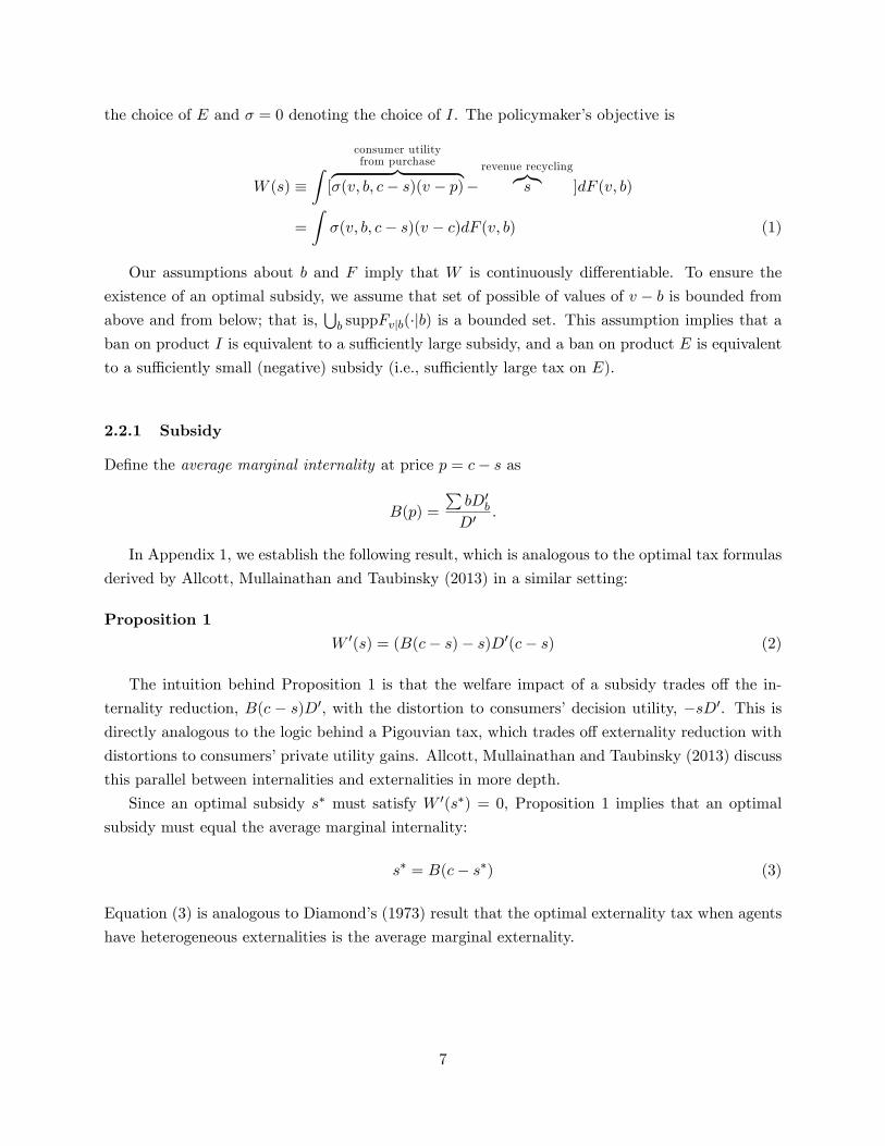
the choice of E and � = 0 denoting the choice of I. The policymaker�s objective is

W (s) �Z[

consumer utilityfrom purchasez }| {

�(v; b; c� s)(v � p)�revenue recyclingz}|{

s ]dF (v; b)

=

Z�(v; b; c� s)(v � c)dF (v; b) (1)

Our assumptions about b and F imply that W is continuously di¤erentiable. To ensure the

existence of an optimal subsidy, we assume that set of possible of values of v � b is bounded fromabove and from below; that is,

Sb suppFvjb(�jb) is a bounded set. This assumption implies that a

ban on product I is equivalent to a su¢ ciently large subsidy, and a ban on product E is equivalent

to a su¢ ciently small (negative) subsidy (i.e., su¢ ciently large tax on E).

2.2.1 Subsidy

De�ne the average marginal internality at price p = c� s as

B(p) =

PbD0bD0

:

In Appendix 1, we establish the following result, which is analogous to the optimal tax formulas

derived by Allcott, Mullainathan and Taubinsky (2013) in a similar setting:

Proposition 1W 0(s) = (B(c� s)� s)D0(c� s) (2)

The intuition behind Proposition 1 is that the welfare impact of a subsidy trades o¤ the in-

ternality reduction, B(c � s)D0, with the distortion to consumers�decision utility, �sD0. This isdirectly analogous to the logic behind a Pigouvian tax, which trades o¤ externality reduction with

distortions to consumers�private utility gains. Allcott, Mullainathan and Taubinsky (2013) discuss

this parallel between internalities and externalities in more depth.

Since an optimal subsidy s� must satisfy W 0(s�) = 0, Proposition 1 implies that an optimal

subsidy must equal the average marginal internality:

s� = B(c� s�) (3)

Equation (3) is analogous to Diamond�s (1973) result that the optimal externality tax when agents

have heterogeneous externalities is the average marginal externality.

7

2.2.2 Ban

In our framework, a ban on good I is equivalent to a su¢ ciently large subsidy for good E. Bans

are thus weakly worse than the optimal subsidy in our model. But when does a ban do better than

the no-intervention benchmark?

According to welfare equation (1), a ban on good I has the following e¤ect on welfare:

�W =

Z(v � c)dF (v; b)�

Z�(v; b; c)(v � c)dF (v; b)

=

Z(1� �(v; b; c))(v � c)dF (v; b)

=

Zf(v;b)j�(v;b;c)=0g

vdF (v; b)� c (4)

This equation simply states that the welfare e¤ects of a ban are the average relative true utility

v for consumers currently purchasing I, minus the relative cost c. An analogous equation would

hold for a ban on E.

2.3 Su¢ cient Statistics for Optimal Subsidies

When the policymaker can directly measure the distribution of consumer types (v; b), welfare can

be computed at each subsidy level to exactly compute the globally optimal subsidy. The TESS

experiment was speci�cally designed to do this. However, this joint distribution is di¢ cult to

estimate: there are only a few papers in any context that cleanly identify biases for even some

subset of consumers. We now detail one approach to approximating the marginal internality using

two reduced form su¢ cient statistics: the slope of demand and the e¤ect of the bias on market

shares. We will later implement this approach for policy analysis using the in-store experiment.

To a �rst order approximation, we have

DRb (p)�Db(p) = Db(p� b)�Db(p)

� bD0b(p)

and thus

DR(p)�D(p) =Xb

(Db(p� b)�Db(p)) �Xb

bD0b = D0(p)B(p)

from which it follows that

B(p) � DR(p)�D(p)D0(p)

: (5)

Alternatively, since (DRb )0(p) = D0b(p � b) � D0b(p) to a �rst-order approximation, we can also

8

approximate B by

B(p) � DR(p)�D(p)(DR)0(p)

: (6)

Figure 1 illustrates the intuition behind Equation (6) for linear demand curves. The length

of segment ab is given by DR(p) � D(p). This could be identi�ed through a randomized �eldexperiment that debiases consumers and measures the e¤ects on demand for E. The demand slope

(DR)0(p) could be identi�ed through an RCT that randomizes relative prices. The segment bd,

which corresponds to the average marginal internality, is given by DR(p)�D(p)(DR)0(p)

. Thus, the e¤ect

of the bias on market shares and the slope of demand are "su¢ cient statistics" for the optimal

subsidy, in the sense of Chetty (2009). Combining Equations (5) and (6) with Equation (3) yield

approximations to the optimal subsidy.

2.4 Measuring Bias with Informational Interventions

We implement interventions that provide information about and draw attention to energy costs,

as well as the longer lifetimes of CFLs. For policy analysis, it seems natural to assume that these

address informational and attentional biases such as:

1. Biased priors about energy costs or other product attributes, as tested by Allcott (2013),

Attari et al. (2010), Bollinger, Leslie, and Sorensen (2011), and others.

2. Exogenous inattention to energy as a shrouded add-on cost, as in Gabaix and Laibson (2006).

3. Costly or constrained cognition, as in Conlisk (1988), Chetty, Looney, and Kroft (2007),

Gabaix (2012), Gabaix et al. (2006), Reis (2006), Sallee (2012), Sims (2004), and others.

Because the interventions immediately provide information about energy costs and product

lifetimes, this addresses any ine¢ ciencies in models where consumers pay a cost to learn

information. Because energy costs are extremely large relative to purchase prices, this assures

that in any model where consumers pay attention to an incomplete or sparse set of product

attributes, they would consider energy costs.

4. "Bias toward concentration," as in Koszegi and Szeidl (2013). Because the interventions

aggregate a stream of future energy payments into one present discounted value, they address

biases in which consumers underweight series of small costs.

To the extent that the bias b is due to the informational and attentional biases above, we assume

that our interventions transform the biased demand curve D into the unbiased demand curve DR.

An important limitation of our interventions, however, is that they do not a¤ect present bias, as in

Laibson (1997), Strotz (1956), and others. This is a plausible bias that could a¤ect choices between

incandescents and CFLs: because energy costs are delayed, present bias would cause consumers

to discount the CFL�s reduced energy costs relative to their long-run preferences. Furthermore,

9

consumers could be imperfectly informed about or inattentive to other attributes not discussed in

our informational interventions. Appendix 1 generalizes the theoretical analysis to the case when

the intervention identi�es only part of the internality. Intuitively, the optimal subsidy is additive in

the di¤erent types of internality. If present bias reduces marginal consumers�demand for the CFL,

then the true optimal subsidy is larger than the subsidies we calculate based on the informational

interventions alone. Similarly, if present bias reduces inframarginal consumers�CFL demand, then

the true welfare e¤ects of a ban are less negative than we calculate.

Finally, note that if an informational intervention that fully debiases consumers were cost ef-

fective and feasible at large scale, it would likely be preferred to a subsidy or ban if the bias b is

heterogeneous. In contrast to a perfectly targeted informational intervention, a (uniform) subsidy

s is less e¢ cient: if it perfectly corrects the choice of consumers with bias b, it still leaves consumers

with bias b0 > b to underpurchase E, while leading consumers with bias b00 < b to overpurchase

E. This is the intuition for why "asymmetric paternalism" (Camerer et al. 2003) and "nudges"

(Sunstein and Thaler 2003) are better targeted corrective policies than a (uniform) subsidy s. How-

ever, our informational interventions are unlikely to be cost e¤ective at scale: even at relatively

high-volume locations, the in-store experiment required labor costs of several dollars per customer

intercept, and both interventions required several minutes of each consumer�s time.

3 In-Store Experiment

3.1 Experimental Design

We partnered with a large home improvement retailer to implement the in-store experiment. Be-

tween July and November 2011, three research assistants (RAs) worked in four stores, one in Boston,

two in New York, and one in Washington, D.C. The RAs approached customers in the stores�"gen-

eral purpose lighting" areas, which stock incandescents and CFLs that are substitutable for the

same uses.7 They told customers that they were from Harvard University and asked, "Are you

interested in answering some quick research questions in exchange for a discount on any lighting

you buy today?" Customers who consented were given a brief survey via iPad in which they were

asked, among other questions, the most important factors in their lightbulb purchase decision, the

number of bulbs they were buying, and the amount of time each day they expected these lightbulbs

to be turned on each day. The survey did not mention electricity costs or distinguish between

incandescents and CFLs.

The iPad randomized customers into treatment and control groups with equal probability. For

the treatment group, the iPad would display the annual energy costs for the bulbs the customer

was buying, given his or her estimated daily usage. It also displayed the total energy cost di¤erence

over the bulb lifetime and the total user cost, which included energy costs plus purchase prices.7This includes standard bulbs used for lamps and overhead room lights. Specialty bulbs like Christmas lights and

other decorative bulbs, outdoor �oodlights, and lights for vanity mirrors are sold in an adjacent aisle.

10

Appendix 2 presents the information treatment screen. The RAs would interpret and discuss the

information with the customer, but they were instructed not to advocate for a particular type of

bulb and to avoid discussing any other issues unrelated to energy costs, such as mercury content

or environmental bene�ts. The control group did not receive this informational intervention, and

the RAs did not discuss energy costs or compare CFLs and incandescents with these customers.

At the end of the survey and potential informational intervention, the RAs gave customers a

coupon in appreciation for their time. The iPad randomized respondents into either the Standard

Coupon group, which received a coupon for 10 percent o¤ all lightbulbs purchased, or the Rebate

Coupon group, which received the same 10 percent coupon plus a second coupon valid for 30 percent

o¤ all CFLs purchased. Thus, the Rebate Coupon group had an additional 20 percent discount on

all CFLs. For a consumer buying a typical package of 60 Watt bulbs at a cost of $3.16 per bulb,

this maps to an average rebate of $0.63 per bulb. The coupons had bar codes which were recorded

in the retailer�s transaction data as the customers submitted them at the register, allowing us to

match the iPad data to purchases.

After giving customers their coupons, the RAs would leave the immediate area in order to avoid

any potential external pressure on customers�decisions. The RAs would then record additional

demographic information on the customer, including approximate age, gender, and ethnicity. The

RA also recorded the total duration of the interaction. The di¤erence between treatment and

control, which had a mean of 3.17 minutes and a median of 3.0 minutes, re�ects the amount of time

spent discussing the energy cost information and the di¤erences between incandescents and CFLs.

3.2 Data and Empirical Strategy

Column 1 of Table 1 presents descriptive statistics for the set of customers who completed the iPad

survey. Columns 2 and 3 present di¤erences between the information treatment and control groups

and between the rebate and standard coupon groups. In one of the 18 t-tests, a characteristic

is statistically di¤erent with 95 percent con�dence: we have slightly fewer Asian people in the

information treatment group. F-tests fail to reject that the groups are balanced.

Our theoretical framework does not include an outside option: all consumers buy either the

incandescent or the CFL. To remain consistent with and to otherwise maintain simplicity, we restrict

our regression sample and welfare analysis to the set of consumers that purchase a "substitutable

lightbulb," by which we mean either a CFL or any incandescent or halogen that can be replaced with

a CFL. The bottom panel of Table 1 shows that 77 percent of interview respondents purchased

any lightbulb with a coupon, and 73 percent of survey respondents purchased a substitutable

lightbulb. While information or rebates theoretically could a¤ect whether or not customers purchase

a substitutable lightbulb, t-tests show that in practice the percentages are not signi�cantly di¤erent

between the groups.

In Section 2, we showed how the average marginal internality could be estimated using two

su¢ cient statistics: the demand response (DR)0(p) or D0(p) and the treatment e¤ect of information.

11

We denote Ti and Si as indicator variables for whether customer i is in the information treatment

and rebate groups, respectively. Xi is the vector of individual-level covariates. We estimate a linear

probability model with robust standard errors using the following equation:

1(Purchase CFL)i = �TTiSi + �C(1� Ti)Si + �Ti + �Xi + "i (7)

3.3 Results

Column 1 of Table 2 presents estimates of Equation (7). For customers who received the standard

coupon and were in the information control group, the CFL market share is 34 percent. The rebate

increases CFL market share by 8 percent in control and by 13 percent in treatment. Column 2 tests

whether these numbers are statistically di¤erent. Because this test fails to reject equality (p=0.41),

and because we have no strong prior about whether the slope of demand should di¤er between

treatment and control, column 3 assumes that the rebate e¤ect is the same in both groups. Theb� from this column implies that the rebate increases CFL market share by ten percentage points.

This implies a price elasticity of demand for CFLs of �Q=Q�P=P � 0:1=0:34�0:2 � �1:5. Column 4 shows

that the results in column 3 are robust to excluding individual level covariates Xi.

The informational intervention does not statistically a¤ect CFL market share. In column 3,

the 90 percent con�dence interval is [-0.050,0.058]. This means that we can reject with 90 percent

con�dence that the intervention had more than two-thirds the estimated e¤ect of the 20 percent

CFL rebate.

3.4 Policy Analysis

For policy analysis, we now make the key assumption that the informational intervention exactly

identi�es the magnitude of the bias, so b� = DR(p) � D(p). Based on the theoretical �rst-orderapproximation and the statistical failure to reject that D0 6= (DR)0, we also assume that b�=s =D0 = (DR)0. Plugging b� , s, and b� from column 3 of Table 2 into Equation (5), the optimal subsidy

per 60-Watt bulb is:

B(S = 0) � DR(p)�D(p)D0(p)

: =b�b�=s � 0:004

0:105=$0:63� $0:024 (8)

Using the Delta method and the estimated variance-covariance matrix, the 90 percent con�dence

interval on the optimal subsidy is (�$0:30; $0:35). The bounds of this con�dence interval increasewith bulb wattage, as higher-wattage bulbs cost more. For comparison, typical CFL rebates o¤ered

by electricity utilities are on the order of $1 to $2 per bulb, and they typically do not depend on

wattage.

Home improvement retailers are the most common place where households buy lightbulbs (DOE

2010), and our partner sells upwards of 50 million packages of lightbulbs each year. Internally valid

12

estimates for our experimental population are thus of great interest per se, and this is why we

chose this particular experimental environment. However, we question whether the results would

generalize to other types of retailers. One particular threat to external validity is that home

improvement stores tend to have relatively good information displayed about lightbulb energy

costs. Our control group might therefore be better informed and more attentive than consumers

at other types of retailers, which could make our treatment e¤ects smaller.

4 TESS Experiment

The in-store �eld experiment is useful because it demonstrates how a simple experimental design

can give su¢ cient statistics which can be used to approximate optimal subsidies. However, this

approach relies on linear approximations of the demand curves, becomes problematic with the

average marginal internality varies with the price. For example, it could be that the consumers

with the lowest willingness to pay have low WTP precisely because they are the most biased. To set

the optimal subsidy, we would ideally calculate welfare directly via Equation (1), using knowledge

of the joint distribution of b and v. Furthermore, we cannot use Equation (4) to analyze the welfare

e¤ects of banning traditional incandescent lightbulbs without knowing the true relative utility for

consumers who would purchase the incandescent in the absence of the ban. Intuitively, we would

like to have all consumers choose in their initial (potentially-biased) state, then debias consumers,

and then observe willingness to pay in the debiased state. To do this, we use what Levitt and

List (2009) call an "artefactual �eld experiment," which studies choices by people in the market of

interest (instead of college students or other typical laboratory experimental subjects), but in an

arti�cial (instead of in-store) environment.

4.1 Survey Platform

We implement the artefactual �eld experiment through Time-Sharing Experiments for the Social

Sciences (TESS). TESS, which is funded by the National Science Foundation, facilitates academic

access to KnowledgePanel, an online experimental platform managed by a company called GfK.

The platform has been used in a number of papers published in economics journals, including Fong

and Luttmer (2009), Heiss, McFadden, and Winter (2007), Newell and Siikamaki (2013), Rabin

and Weizsacker (2009), and our own previous work (Allcott 2013).

One reason why economists are use TESS is that the sample is as close as practical to being

nationally representative on unobservable characteristics. Potential KnowledgePanel participants

are randomly selected from the U.S. Postal Service Delivery Sequence File and recruited through

a series of mailings in English and Spanish, plus telephone-based follow-up when the address can

be matched to a phone number. About 10 percent of people who are invited actually consent

and complete the demographic pro�le to become KnowledgePanel participants, and there are now

13

approximately 50,000 active panel members. Unrecruited volunteers are not allowed to opt in.

Households without computers are given computers in order to complete the surveys.

KnowledgePanel participants take an average of two studies per month, and no more than

one per week. Of the KnowledgePanel participants invited to participate in our study, about 60

percent completed it. All results in the text, tables, and �gures weight observations to match the

US population aged 18 and older on gender, age, ethnicity, education, census region, urban or rural

location, and whether the household had internet access before recruitment.

Note that in this draft, we do not yet have the weights or �nal response rates. Thus, the numbers

will change (slightly) in future drafts.

4.2 Experimental Design

The study had four parts: baseline lightbulb choices, the informational intervention, endline light-

bulb choices, and a post-experiment survey. Appendix 3 contains screen shots from each part of

the experiment.

Consumers were �rst shown an introductory screen with the following text:

In appreciation for your participation in this study, we are giving you an $8 shopping budget.

With this money, we will o¤er you the chance to buy light bulbs. You must make a purchase with

this money. Whatever money you have left over after your purchase, you get to keep. This money

will be provided to you as cash-equivalent bonus points that will be awarded to your account.

In approximately four to six weeks, GfK will send you the light bulbs you have purchased. Light

bulbs are frequently shipped in the mail. There is not much risk of breakage, but if anything does

happen, GfK will just ship you a replacement. Even if you don�t need light bulbs right now, remember

that you can store them and use them in the future.

During the study, we will ask you to make 26 decisions between pairs of light bulbs. There will

be a �rst set of 13 decisions, then a break, and then a second set of 13 decisions. After you �nish

with all 26 decisions in the questionnaire, one of them will be randomly selected as your �o¢ cial

purchase.�GfK will ship you the light bulbs that you chose in that o¢ cial purchase. Since each of

your decisions has a chance of being your o¢ cial purchase, you should think about each decision

carefully.

4.2.1 Baseline Lightbulb Choices

After the introductory screen, consumers were then shown two lightbulb packages. One package

contained one Philips 60-Watt equivalent Compact Fluorescent Lightbulb. The other contained

four Philips 60-Watt incandescent lightbulbs. Each package typically retails online for about $4.

The two choices were chosen to be as comparable as possible, except for the CFL vs. incandescent

technology. Half of respondents were randomly assigned to see the incandescent on the left, labeled

as "Choice A," while the other half saw the incandescent on the right, labeled as "Choice B."

14

Consumers had the option to "click for detailed product information," and about 17 percent did

so. This opened a simple "Detailed Product Information" screen, which included the normal retail

price, light output in Lumens, color temperature, energy use in Watts, and the manufacturer�s

home country.

Lower down on this same screen, consumers were asked to make their baseline lightbulb choices:

13 decisions between the same two packages at di¤erent relative prices. To implement the di¤erent

prices, we told consumers that the price you pay for the bulb is the normal retail price, which is

$4, minus any instant rebate or plus any additional tax. Decision Number 1 o¤ered Choice A for

free (after $4 instant rebate) and Choice B for $8 (including $4 additional tax). The relative price

of Choice A increased monotonically until Decision Number 13, which o¤ered Choice A for $8

(including $4 additional tax) and Choice B for free (after $4 instant rebate). Consumers spent a

median of three minutes and 52 seconds to complete these 13 decisions.

We identify consumers�baseline relative willingness to pay (WTP) for the CFL, denoted v0i ,

using the relative prices at which they switch from preferring CFLs to incandescents. For example,

consumers who choose CFLs when both packages cost $4 but choose incandescents when incandes-

cents are one dollar cheaper are assumed to have v0i = $0:50. Nine percent of consumers did not

choose monotonically: they chose Choice A at a higher relative price than another decision at which

they chose Choice B. These consumers were prompted with the following message: The Decision

Numbers below are organized such that Choice A costs more and more relative to Choice B as you

read from top to bottom. Thus, most people will be more likely to purchase Choice A for decisions

at the top of the list, and Choice B for decisions at the bottom of the list. Feel free to review your

choices and make any changes. Then click NEXT. After this prompt, 7.4 percent of consumers

still chose non-monotonically, and we code their WTP as missing.

Some consumers had "top-coded" WTPs: they preferred either Choice A or Choice B at all

relative prices. These consumers were asked to self-report their WTP. For example, a participant

who always preferred Choice A was asked: Your decisions suggest that you prefer Choice A even

when Choice A costs a total of $8 and Choice B is free. If Choice B continued to be free, how much

would Choice A need to cost in order for you to switch to Choice B? (This is purely hypothetical -

your answer will not a¤ect any of the prices you are o¤ered.)

Four percent of consumers preferred the incandescents by more than $8, while 21 percent pre-

ferred the CFLs by more than $8. Among both of these "top-coded" groups, the median self-

reported relative WTP was $10. However, the distribution of self-reports is highly skewed, with

about four percent of top-coded consumers preferring one or the other choice by more than $100.

Because these are self-reports, we wish to be cautious about using them in the analysis, so we

instead assume a relative WTP of $10 for all top-coded consumers.

15

4.2.2 Informational Intervention

Respondents were randomized into three groups with equal probability: Balanced treatment, Pos-

itive treatment, and control. The information treatments were designed to give clear product

information while avoiding possible perceived bias.

The treatments were also designed to closely parallel each other, to minimize the chance that

idiosyncratic factors other than the information content could a¤ect purchases. Each treatment

had the following structure:

1. Belief elicitation. This elicited prior beliefs over the information to be presented in the two

Information Screens.

2. Introductory Screen

3. First Information Screen. This had text plus an illustratory graph, and the text was also

read verbatim via an audio recording. The audio recordings are available as part of the

Online Supplementary Materials. KnowledgePanel members were not allowed to participate

in the study unless they con�rmed that their computer audio worked. At the bottom of the

information screen, there was a "quiz" on a key fact.

4. Second Information Screen. This paralleled the �rst screen.

Each of the three groups had two particular Information Screens to be presented. The order of

these two screens was randomly assigned with equal probability.

We took two steps to make sure that all consumers understood the treatment. First, we used

multiple channels to convey information: text, graphical, and audio. This means that people who

process information in di¤erent ways had a higher chance of internalizing the information. Second,

the quiz forced respondents to internalize the information if they had not done so initially. This

quiz is also useful because it allows us to document the extent to which consumers eventually

understood the information.

Balanced Treatment The Balanced treatment Introductory Screen had the following text:

For this next part of the study, you will have the opportunity to learn more about light bulbs.

We will focus on the following two issues:

1. Total Costs

2. Disposal and Warm-Up Time

The discussion of each issue will be followed by a one-question quiz. Please pay close attention

to the discussion so that you can correctly answer the quiz question.

16

Consumers then advanced to the Total Cost Information Screen and the Disposal and the Warm-

Up Information Screen, in randomized order. The Total Cost Information Screen explained that

CFLs both last longer and use less electricity and translates these di¤erences into dollar amounts.

The bottom line was:

Thus, for eight years of light, the total costs to purchase bulbs and electricity would be:

� $56 for incandescents: $8 for the bulbs plus $48 for electricity.

� $16 for a CFL: $4 for the bulbs plus $12 for electricity.

The quiz question at the bottom of the screen was: For eight years of light, how much larger

are the total costs (for bulbs plus electricity) for 60-Watt incandescents as compared to their CFL

equivalents? The correct answer could be inferred from the information on the screen: $56 for

incandescents - $16 for CFLs = $40. Sixty-eight percent of consumers correctly put $40. Those

who did not were prompted: That is not the correct answer. Please try again. After this prompt,

79 percent of consumers had typed $40. The remaining consumers were prompted: The total costs

for eight years of light are $16 for CFLs and $56 for incandescents. Therefore, the incandescents

cost $40 more. You may type the number 40 into the answer box. By this point, 93 percent

of consumers had correctly typed $40. This documents that the vast majority of consumers did

indeed understand at least some part of the information. Consumers spent a median of two minutes

and 15 seconds to read the Total Cost Information Screen and complete the quiz question.

The Disposal and Warm-Up Information Screen was designed to present information about

ways in which CFLs may not be preferred to incandescents. It paralleled exactly the Total Cost

Information Screen, beginning with belief elicitation, and then continuing to an Information Screen

with text of similar length, a graph, and a quiz question at the bottom. The Disposal and Warm-Up

Information Screen explained that "because CFLs contain mercury, it is recommended that they be

properly recycled instead of disposed of in regular household trash." It also explained that "after

the light switch is turned on, CFLs take longer to warm up than incandescents." We included this

module to reduce the probability of experimenter demand e¤ects: that consumers would think that

the experimenter wanted them to purchase one or the other type of lightbulb, and that this would

a¤ect their purchases.

Control The control intervention was designed to exactly parallel the treatment interventions,

but with information that should not a¤ect relative WTP for CFLs vs. incandescents. One screen

presented the number of lightbulbs installed in residential, commercial, and industrial buildings in

the United States. The other screen detailed trends in total lightbulb sales between 2000 and 2009.

17

Positive Treatment The Positive treatment was designed to inform consumers about the ben-

e�ts of the CFL in terms of lifetime and lower energy costs, without presenting information about

ways that the incandescent might be preferred to the CFL. To implement this while keeping the

intervention the same length, we combined the Total Cost Information Screen with one module

randomly selected from the two control screens.

4.2.3 Endline Lightbulb Choices

The endline lightbulb choice screen was analogous to the baseline screen, except that consumers

who had the CFL as Choice A in the baseline choice screen now had it as Choice B, and vice versa.

We switched the order of the choices in order to help address any mechanical anchoring on past

choices or bias towards consistency with past choices. Consumers spent a median of one minute

and 37 seconds to complete these �nal 13 decisions.

We determine endline relative WTP v1i in the same way as above. Top coding of endline relative

WTP is especially important for our policy analysis, as we interpret the imputed top-coded value of

$10 as the consumer�s true v. The skewness of the WTP distribution could cause us to understate

the welfare costs of banning incandescents, because we would understate the strength of preferences

for incandescents at the tail of the WTP distribution. On the other hand, the informational

treatment caused a small share of inframarginal consumers who purchased incandescents at baseline

to decide that they prefer CFLs by more than $8. If these top-coded positive valuations are very

large, our results could overstate the welfare costs of the ban.

4.3 Data and Empirical Strategy

Column 1 of Table 3 presents descriptive statistics for the TESS experimental population. Like all

other results from the TESS experiment, these are weighted for national representativeness. Liberal

is self-reported political ideology, originally on a seven-point scale, normalized to mean zero and

standard deviation one, with larger numbers indicating more liberal. Similarly, Party is self-reported

political a¢ liation, also originally on a seven-point scale, normalized to mean zero and standard

deviation one, with larger numbers indicating more strongly Democratic. Environmentalist is the

consumer�s answer to the question, "Would you describe yourself as an environmentalist?" Conserve

Energy is an indicator for whether the consumer reports having taken steps to conserve energy in the

past twelve months. These questions were asked when the participant �rst entered KnowledgePanel,

not as a part of our experiment.

Column 2 presents the di¤erence in means between consumers in either of the two treatment

groups vs. control. Column 3 presents the di¤erence in means between the Positive and Balanced

treatment groups. All of the 16 t-tests fail to reject equality, as the joint F-test of all characteristics.

18

Denote Xi as participant i�s vector of characteristics from Table 3, and Ti as an indicator

for whether the household is in either of the two treatment groups. We estimate the e¤ects of the

informational interventions on endline willingness-to-pay v1i using OLS with robust standard errors:

v1i = �Ti + Xi + "i (9)

4.4 Empirical Results

Table 4 presents estimated e¤ects of the informational interventions. Column 1 tests whether the

e¤ects of the information treatments are statistically di¤erent, and the test fails to reject equality.

We therefore group all treated consumers together for the remainder of the analysis. Column 2 is

the exact speci�cation from Equation (9). The informational intervention caused consumers�WTP

for the CFL to increase by an average of $1.12. Column 3 omits all individual X characteristics

other than baseline WTP v0i , while column 4 also omits v0i . The sample sizes increase somewhat

because X characteristics are missing for a small number of consumers, but the e¤ects do not

change statistically.

The post-experiment survey asked consumers what they thought the intent of the study was.

Multiple responses were allowed. The top panel of Table 5 presents the share of each treatment

group that gave each response. None of the responses di¤er between the two treatment groups.

However, the treatment groups were more likely to respond that the intent of the study was to

understand why people buy incandescents vs. CFLs, persuade people to buy CFLs, or educate

people about lightbulbs. The treatment groups were less likely to respond that the intent was to

understand the e¤ects of rebates and taxes, test whether the number of bulbs in a package a¤ects

purchasing patterns, and predict the future popularity of incandescents vs. CFLs.

Only for consumers that responded that the intent of the study was to persuade people to

buy either incandescents or CFLs, we asked if this a¤ected their purchase decisions. The bottom

panel of Table 5 presents responses. Of the treatment group consumers who were asked this

question, about 40 percent responded that they had been more likely to purchase the CFL. We are

not certain how consumers interpreted this question. Some consumers may have meant that the

information in the treatment increased their WTP for the CFL, which would be consistent with

the interpretation of the treatment e¤ect as a measure of bias. Others may have meant that the

treatment acted as persuasive advertising in the sense of Becker and Murphy (1993), or that their

beliefs about the intent of the study directly caused them to change their purchase decisions. Such

persuasive advertising e¤ects or experimenter demand e¤ects would confound the interpretation of

the treatment e¤ect as a measure of internalities.

One way to quantify these e¤ects is to condition on perceived intent of the study when estimating

treatment e¤ects. If the treatment acts by a¤ecting consumers� perceived intent, and di¤erent

perceived intents cause consumers to make di¤erent choices, the estimated treatment e¤ects will

19

change. If the treatment e¤ects do not change, this suggests that the intervention does not act

through experimenter demand e¤ects. However, such regressions should be interpreted cautiously, as

they include endogenous regressors that are directly a¤ected by the treatment. Results are included

in Appendix 4, as Table A4-1. The coe¢ cients on the treatment variable remain statistically

signi�cant, and they are not statistically signi�cantly di¤erent from the main results. However, the

point estimates drop slightly toward zero. To the extent that these issues cause us to overstate

the extent of informational and attentional biases, this strengthens the qualitative conclusion that

such biases do not justify a ban on incandescent lightbulbs.

How much of the treatment e¤ect is from changing information sets vs. drawing attention?

The post-experiment survey elicits beliefs over how much less it costs to buy electricity for a CFL

vs. incandescents over the typical 8000-hour life of a CFL, at national average electricity prices.

The question is similar, but not identical to, the "quiz" question asked of the treatment group, and

the correct answer is $36 ($48 for the incandescent minus $12 for the CFL). Column 1 of Table

6 shows that the treatment increases median beliefs: they are $26 in control and $14 higher in

treatment. Column 2 of Table 6 shows that the treatment also substantially reduces the median

absolute error, i.e. the absolute value of the di¤erence between the reported belief and $36. We use

median regressions because reported beliefs have high variance, and median regressions are more

robust to extreme outliers than OLS. These results suggest that at least part of the treatment e¤ects

could be from changing information sets. In Appendix 4, Table A4-2 also shows that the treatment

increased the self-reported importance of energy use and bulb lifetime in purchase decisions.

Does present bias play a role in consumers� lightbulb choices? Consider a quasi-hyperbolic

(�; �) model as in Laibson (1997), where � is the long-run discount rate and � is the present bias

parameter. In the post-experiment survey, we estimate � and � through a menu of hypothetical

intertemporal choices at two di¤erent time horizons: $100 now vs. $m1i in one year, and $100 in

one year vs. $m2i in two years. Denoting bm1 and bm2 as the minimum values at which participant i

prefers money sooner, the long run discount factor is �i = 1=bm2, and the present bias parameter is

�i = bm2i =bm1

i . We dropped non-monotonic responses and top-coded bm1 and bm2 in a similar fashion

to how we constructed v0 and v1.

If there is a distribution of �, consumers with lower � (more present bias) should be more likely

to purchase incandescents. In regressions presented in Appendix 4, Table A4-3, there is some weak

evidence (p = 0:16 at best) that � is associated with baseline WTP v0i , suggesting that people who

are more patient are more likely to purchase CFLs. However, there is no statistically signi�cant

correlation between � and v0i (p = 0:52 at best), and we can rule out with 90 percent con�dence

that a one standard deviation increase in � is associated with more than a $0.54 increase in v0i .

Because these intertemporal choices were hypothetical, not incentive compatible, we view this only

as some initial suggestive evidence that present bias may not justify policies to promote energy

e¢ cient lighting, and certainly not a primary feature of this paper.

As discussed earlier, one bene�t of the TESS experimental design is that we can explicitly trace

20

out the joint distribution of b and v0, to test whether the marginal internality di¤ers at di¤erent

relative prices. Figure 2 presents the treatment e¤ects as a function of baseline WTP. (There are

only a small number of consumers with v0 of $-7 or $7, so the standard errors at these points are

large.) The treatment e¤ects appear to be fairly constant across the graph, and an F-test fails to

reject equality (p=0.86).

4.5 Policy Analysis

For policy analysis, we again assume that the treatment e¤ect of the informational intervention

identi�es that magnitude of the bias. Table 7 uses the TESS data to evaluate the welfare e¤ects of

di¤erent levels of subsidy for a 60-Watt CFL. Column 1 contains the subsidy amount. Column 2

presents the average baseline relative WTP v0 for consumers marginal to the increase in the subsidy

relative to the row above, assuming that demand is linear between the two price levels. Column

3 presents the average internality for this group of marginal consumers. Graphically, this is the

treatment e¤ect for each point on the left side of Figure 2. Column 4 presents the demand density:

the share of all consumers that are marginal at each relative price level. Column 5 presents the

welfare e¤ect of the increment to the subsidy, using Equation (1), while column 6 presents the total

welfare e¤ect of changing the subsidy from zero to the amount listed in that row. Columns 3-6 are

measured with sampling error, although we omit standard errors for simplicity. Again, this welfare

calculation assumes that subsidy funds are raised through non-distortionary taxes, informational

and attentional biases are the only distortion, and the TESS treatment e¤ects exactly measure this

distortion.

The table has units denominated in "packages," which refers to consumers�choice between either

one package of four incandescents or one package of one CFL. Increasing the subsidy from zero to

one dollar increases welfare by $0.074 per package. In 2009, there were 1.47 billion incandescent

bulbs and 310 million CFLs sold (DOE 2010), which translates to a total of 677 million "packages."

Thus, a nationwide CFL subsidy of $1 per bulb would have increased welfare by $50 million dollars

in that year.

As Equation (2) shows, a marginal increase in the subsidy increases welfare as long as the

marginal internality outweighs the distortion to decision utility. Table 7 shows that for subsidies

larger than one dollar, the point estimate of the marginal internality is always less than v0i . Thus,

an incremental increase in the subsidy to $2 or more will reduce welfare. Extending the analogy

to externalities, these higher subsidies are equivalent to setting a Pigouvian externality tax higher

than marginal external damages.

The bene�t of this "grid search" approach to calculating the optimal subsidy is that in theory,

the average marginal internality could be very di¤erent for di¤erent values of v0. Grid search

identi�es the global optimum even if the necessary condition for a local optimum in Equation (3)

is satis�ed at multiple places. Above, however, we found no statistical evidence B(p) varies with

21

p. If we assume that the average marginal internality at all p equals the average treatment e¤ectb� = $1:12, Equation (3) implies that the globally optimal subsidy is also s� = $1:12.An incandescent lightbulb ban is equivalent to a change in relative prices that is so large as to

induce all consumers to cease buying incandescents. In Table 7, given the bottom-coding of relative

WTP for the CFL at $-10, a $10 CFL subsidy is equivalent to a ban on incandescents. This reduces

welfare by $0.55 per package, or $371 million across all "packages" sold in 2009.

5 Conclusion

One potential reason to subsidize energy e¢ cient lightbulbs or ban traditional incandescents is that

imperfect information or attentional biases could cause consumers to overpurchase incandescents

relative to their private optima. In this paper, we formalize a model of optimal policy that allows

for such biases. We then present results from two �eld experiments designed to inform consumers

about the total costs of di¤erent lightbulb technologies. The treatment e¤ects could provide support

for moderate subsidies: no more than $0.35 cents per 60-Watt equivalent CFL from the in-store

experiment, and a point estimate of $1.12 in the TESS experiment. However, these experiments

provide no evidence to suggest that a ban on traditional incandescent lightbulbs would increase

welfare.

Because our analysis relates to a potentially controversial policy question, it is important to

re-emphasize the limitations of this analysis. Our interventions were designed to debias consumers

subject to informational and attentional biases, which we believe could be a leading potential

justi�cation for intervention. However, aside from some initial suggestive evidence that present bias

may not play a large role in lightbulb decisions, our analysis provides no evidence on other potential

justi�cations. Our model and �eld experiments assume away technological change, so we also

provide no evidence on how potential advances in light-emitting diodes or advanced incandescents

might change the welfare calculation.

Furthermore, in mapping experimental results to formal policy analysis, we assume that the

intervention fully debiases consumers, and has no other e¤ects. If the treatments also acted through

experimenter demand e¤ects or other forms of persuasion or social pressure, this would change our

interpretation - although if such e¤ects increase CFL market share in the treatment group, this

only strengthens the qualitative result that an incandescent lightbulb ban reduces welfare. Fur-

thermore, external validity is a potential concern when generalizing from these experimental results

to national-level policy. However, the in-store �eld experiment takes place in home improvement

stores, which are the modal place where households buy lightbulbs, while the TESS experiment

uses consumers from all 50 states and is as representative as practically possible for a sample survey.

Although we have focused our application on one particularly important and controversial

policy, the approach is quite general. Our theoretical framework generalizes immediately to any

binary or continuous choice, and the idea of using informational interventions in RCTs to quantify

22

internalities can be used in a wide variety of contexts. The approach to optimal policy could be

useful in other contexts where informational or attentional biases might be used to justify subsidies

or bans and where informational interventions can debias consumers in small RCTs, but would not

be cost-e¤ective to implement on a large scale. Such contexts might include regulation of �nancial

products like credit cards or mortgages, incentives for preventive health measures such as screening

tests, and health regulations like bans on trans fats or large soft drinks.

23

References

[1] Allcott, Hunt (2011). "Consumers�Perceptions and Misperceptions of Energy Costs." American Eco-nomic Review, Vol. 101, No. 3 (May), pages 98-104.

[2] Allcott, Hunt (2013). "The Welfare E¤ects of Misperceived Product Costs: Data and Calibrations fromthe Automobile Market." American Economic Journal: Economic Policy, forthcoming.

[3] Allcott, Hunt, and Michael Greenstone (2012). "Is there an Energy E¢ ciency Gap?" Journal of Eco-nomic Perspectives, Vol. 26, No. 1 (Winter), pages 3-28.

[4] Allcott, Hunt, Sendhil Mullainathan, and Dmitry Taubinsky (2013). "Energy Policy with Externalitiesand Internalities." NBER Working Paper 17977 (June).

[5] Allcott, Hunt, and Nathan Wozny (2013). "Gasoline Prices, Fuel Economy, and the Energy Paradox."Review of Economics and Statistics, forthcoming.

[6] Anderson, Soren, Ryan Kellogg, and James Sallee (2011). "What Do Consumers Believe about FutureGasoline Prices?" NBER Working Paper No. 16974 (April).

[7] Attari, Shahzeen, Michael DeKay, Cli¤ Davidson, and Wandi Bruine de Bruin (2010). "Public Percep-tions of Energy Consumption and Savings." Proceedings of the National Academy of Sciences, Vol. 107,No. 37 (September 14), pages 16054-16059.

[8] Baicker, Kate, Sendhil Mullainathan, and Joshua Schwartzstein (2012). "Choice Hazard in Health In-surance." Working Paper, Dartmouth College (October).

[9] Becker, Gary, and Kevin Murphy (1993). "A Simple Theory of Advertising as a Good or Bad." QuarterlyJournal of Economics, Vol. 108, No. 4 (November), pages 941-964.

[10] Bernheim, B. Douglas, and Antonio Rangel (2004). "Addiction and Cue-Triggered Decision Processes."American Economic Review, Vol. 90, No. 5 (December), pages 1558-1590.

[11] Bernheim, B. Douglas, and Antonio Rangel (2009). "Beyond Revealed Preference: Choice-TheoreticFoundations for Behavioral Welfare Economics." Quarterly Journal of Economics, Vol. 124, No. 1 (Feb-ruary), pages 51-104.

[12] Bhargava, Saurabh, and Dayanand Manoli (2013). "Why Are Bene�ts Left on the Table? Assessingthe Role of Information, Complexity, and Stigma on Take-up with an IRS Field Experiment." WorkingPaper, University of Texas at Austin.

[13] Bollinger, Brian, Phillip Leslie, and Alan Sorensen (2011). �Calorie Posting in Chain Restaurants.�American Economic Journal: Economic Policy, Vol. 3, No. 1 (February), pages 91-128.

[14] Camerer, Colin, Samuel Issacharo¤, George Loewenstein, Ted O�Donoghue, and Matthew Rabin (2003)."Regulation for Conservatives: Behavioral Economics and the Case for Asymmetric Paternalism." Uni-versity of Pennsylvania Law Review, Vol. 151, pages 1211-1254.

[15] Chetty, Raj (2009). "Su¢ cient Statistics for Welfare Analysis: A Bridge Between Structural andReduced-Form Methods." Annual Review of Economics, Vol. 1, pages 451-488.

[16] Chetty, Raj, Adam Looney, and Kory Kroft (2007). "Salience and Taxation: Theory and Evidence."NBER Working Paper 13330 (August).

[17] Chetty, Raj, Adam Looney, and Kory Kroft (2009). "Salience and Taxation: Theory and Evidence."American Economic Review, Vol. 99, No. 4 (September), pages 1145-1177.

[18] Choi, James, David Laibson, and Brigitte Madrian (2011). "$100 Bills on the Sidewalk: SuboptimalInvestment in 401(k) Plans." Review of Economics and Statistics, Vol. 93, No. 3 (August), pages 748-763.

[19] Kling, Je¤rey, Sendhil Mullainathan, Eldar Sha�r, Lee Vermeulen, and Marian Wrobel (2012). "Com-parison Friction: Experimental Evidence from Medicare Drug Plans." Quarterly Journal of Economics.Vol. 127, No. 1, pages 199-235.

24

[20] Conlisk, John (1988). "Optimization Cost." Journal of Economic Behavior and Organization, Vol. 9,No. 3, pages 213-228.

[21] Davis, Lucas, and Erich Muehlegger (2010). "Do Americans Consume too Little Natural Gas? AnEmpirical Test of Marginal Cost Pricing." RAND Journal of Economics, Vol. 41, No. 4 (Winter), pages791-810.

[22] Diamond, Peter (1973). "Consumption Externalities and Imperfect Corrective Pricing." Bell Journal ofEconomics and Management Science, Vol. 4, No. 2 (Autumn), pages 526-538.

[23] DOE (U.S. Department of Energy) 2010. "Energy Star CFL Market Pro�le: Data Trends and MarketInsights." http://www.energystar.gov/ia/products/downloads/CFL_Market_Pro�le_2010.pdf,

[24] DOE (U.S. Department of Energy) 2012. "2010 US Lighting Market Characterization."http://apps1.eere.energy.gov/buildings/publications/pdfs/ssl/2010-lmc-�nal-jan-2012.pdf

[25] Duarte, Fabian, and Justine Hastings (2012). "Fettered Consumers and Sophisticated Firms: Evidencefrom Mexico�s Privatized Social Security Market." NBER Working Paper 18582 (November).

[26] Du�o, Esther, and Emmanuel Saez (2003). "The Role of Information and Social Interactions in Retire-ment Plan Decisions: Evidence from a Randomized Experiment." Quarterly Journal of Economics, Vol.118, No. 3 (August), pages 815-842.

[27] Figlio, David, and Maurice E. Lucas (2004). "What�s in a Grade? School Report Cards and the HousingMarket." American Economic Review, Vol. 94, No. 3, pages 591�604.

[28] Formisano, Bob (2008). "2007 Energy Bill - Are They Phasing Out or Making Incandescent BulbsIllegal?" http://homerepair.about.com/od/electricalrepair/ss/2007_energybill.htm

[29] Gabaix, Xavier (2012). "A Sparsity-Based Model of Bounded Rationality." Working Paper, New YorkUniversity (September).

[30] Gabaix, Xavier, and David Laibson (2006). "Shrouded Attributes, Consumer Myopia, and InformationSuppression in Competitive Markets.�Quarterly Journal of Economics, Vol. 121, No. 2, pages 505-540.

[31] Greenstone, Michael, Paul Oyer, and Annette Vissing-Jorgensen (2006). �Mandated Disclosure, StockReturns, and the 1964 Securities Acts Amendments.�Quarterly Journal of Economics, Vol. 121, No. 2,pages 399�460.

[32] Gul, Faruk, and Wolfgang Pesendorfer (2007). "Harmful Addiction." Review of Economic Studies, Vol.74, No. 1 (January), pages 147-172.

[33] Hastings, Justine, and Je¤rey Weinstein (2008).�Information, School Choice, and Academic Achieve-ment: Evidence from Two Experiments.� Quarterly Journal of Economics, Vol. 123, No. 4, pages1373�1414.

[34] Heutel, Garth (2011). "Optimal Policy Instruments for Externality-Producing Durable Goods underTime Inconsistency." Working Paper, UNC Greensboro (May).

[35] Herrnstein, R. J., George Loewenstein, Drazel Prelec, and William Vaughan, Jr. (1993). "Utility Max-imization and Melioration: Internalities in Individual Choice." Journal of Behavioral Decision Making,Vol. 6, pages (149-185).

[36] Houde, Sebastien (2012). "How Consumers Respond to Certi�cation: A Welfare Analysis of the EnergyStar Program." Working Paper, Stanford University (October).

[37] Interagency Working Group on Social Cost of Carbon, United States Govern-ment (2013). "Technical Support Document: Technical Update of the SocialCost of Carbon for Regulatory Impact Analysis Under Executive Order 12866."http://www.whitehouse.gov/sites/default/�les/omb/inforeg/social_cost_of_carbon_for_ria_2013_update.pdf

25

[38] Jensen, Robert (2010). �The Perceived Returns to Education and the Demand for Schooling.�QuarterlyJournal of Economics, Vol. 125, No. 2 (May), pages 515-548.

[39] Jin, Ginger Zhe, and Alan Sorensen (2006). �Information and Consumer Choice: The Value of PublicizedHealth Plan Ratings.�Journal of Health Economics, Vol. 25, No. 2, pages 248�275.

[40] Koszegi, Botond, and Adam Szeidl (2013). "A Model of Focusing in Economic Choice." QuarterlyJournal of Economics, Vol. 128, No. 1, pages 53-107.

[41] Laibson, David (1997). "Golden Eggs and Hyperbolic Discounting." Quarterly Journal of Economics,Vol. 112, No. 2 (May), pages 443-477.

[42] Levitt, Steve, and John List (2009). "Field Experiments in Economics: The Past, the Present, and theFuture." European Economic Review, Vol. 53, pages 1-18.

[43] Mills, Bradford, and Joachim Schleich (2010). "Why Don�t Households See the Light? Explaining theDi¤usion of Compact Fluorescent Lamps." Resource and Energy Economics, Vol. 32, pages 363-378.

[44] NHTSA (National Highway Tra¢ c Safety Administration) (2010). "Final Regulatory Impact Analysis:Corporate Average Fuel Economy for MY 2012-MY 2016 Passenger Cars and Light Trucks." O¢ ce ofRegulatory Analysis and Evaluation, National Center for Statistics and Analysis (March).

[45] Newell, Richard, and Juha Siikamaki (2013). "Nudging Energy E¢ ciency Behavior: The Role of Infor-mation Labels." Resources for the Future Discussion Paper 13-17 (July).

[46] NRDC (Natural Resources Defense Council) 2011. "Better Light Bulbs Equal Consumer Savings inEvery State." www.nrdc.org/policy

[47] O�Donoghue, Edward, and Matthew Rabin (2006). "Optimal Sin Taxes." Journal of Public Economics,Vol. 90, pages 1825-1849.

[48] Parry, Ian, David Evans, and Wallace Oates (2010). "Are Energy E¢ ciency Standards Justi�ed? Re-sources for the Future Discussion Paper 10-59 (November).

[49] Pope, Devin (2009). "Reacting to Rankings: Evidence from �America�s Best Hospitals.�" Journal ofHealth Economics, Vol. 28, No. 6, pages 1154-1165.

[50] Rabin, Matthew, and Georg Weizsacker (2009). "Narrow Bracketing and Dominated Choices." AmericanEconomic Review, Vol. 99, No. 4 (September), pages 1508-1543.

[51] Reis, Ricardo (2006). "Inattentive Consumers." Journal of Monetary Economics, Vol. 53, No. 8, pages1761-1800.

[52] Sallee, James (2012). "Rational Inattention and Energy E¢ ciency." Working Paper, University ofChicago (September).

[53] Scanlon, Dennis, Michael Chernew, Catherine McLaughlin, and Gary Solon (2002). "The Impact ofHealth Plan Report Cards on Managed Care Enrollment." Journal of Health Economics, Vol. 21 No. 1,pages 19-41.

[54] Sims, Christopher (2003). "Implications of Rational Inattention." Journal of Monetary Economics, Vol.50, No. 3, pages 665-690.

[55] Strotz, Robert (1956). "Myopia and Inconsistency in Dynamic Utility Maximization." Review of Eco-nomic Studies, Vol. 23, pages 165-180.

[56] Sunstein, Cass and Richard Thaler (2003). "Libertarian Paternalism is not an Oxymoron." Universityof Chicago Law Review, Vol. 70, No. 4 (Fall), pages 1159-1202.

[57] Ward, David, Christopher Clark, Kimberly Jensen, Steven Yen, and Cli¤ord Russell (2011). �FactorsIn�uencing Willingness-to-Pay for the Energy Star Label.�Energy Policy, Vol. 39, No. 3 (March), page1450 �1458.

26

Tables

Table 1: Descriptive Statistics and Balance for In-Store Experiment

(1) (2) (3)Experimental Treatment - Control Rebate - Standard

Individual Characteristics Population Mean Di¤erence Coupon Di¤erenceEnergy an Important Factor 0.25 0.009 -0.024in Purchase Decision ( 0.43 ) ( 0.026 ) ( 0.026 )

Expected Usage (Minutes/Day) 333 12.8 2.7( 280 ) ( 17.0 ) ( 17.0 )

Age 43.8 0.7 -0.3( 11.4 ) ( 0.7 ) ( 0.7 )

Male 0.66 0.009 0.003( 0.47 ) ( 0.029 ) ( 0.029 )

African American 0.16 -0.001 -0.008( 0.37 ) ( 0.022 ) ( 0.022 )

Asian 0.06 -0.030 0.005( 0.24 ) ( 0.014 )�� ( 0.015 )

Caucasian 0.66 0.037 -0.005( 0.47 ) ( 0.029 ) ( 0.029 )

Hispanic 0.07 0.001 0.011( 0.25 ) ( 0.015 ) ( 0.015 )

Middle Eastern 0.01 0.002 0.007( 0.12 ) ( 0.013 ) ( 0.007 )

F-Test p-Value 0.742 0.896

Purchase DecisionsPurchased Any Lightbulb 0.77 0.011 0.027

( 0.42 ) ( 0.025 ) ( 0.025 )Purchased Substitutable Lightbulb 0.73 -0.008 0.011

( 0.44 ) ( 0.027 ) ( 0.027 )Notes: Column 1 presents means of individual characteristics in the in-store experiment population,

with standard deviations in parenthesis. Columns 2 presents di¤erences in means between treatment andcontrol groups, while column 3 presents di¤erences in means between the rebate and standard coupon groups.Columns 2 and 3 have robust standard errors in parenthesis. *, **, ***: Statistically signi�cant with 90, 95,and 99 percent con�dence, respectively.

27

Table 2: Empirical Results In-Store Experiment

(1) (2) (3) (4)

1(Rebate and Control) 0.078

(0.047)*

1(Rebate and Treatment) 0.132 0.054

(0.046)*** (0.066)

1(Treatment) -0.022 -0.022 0.004 -0.002

(0.045) (0.045) (0.033) (0.035)

1(Rebate) 0.078 0.105 0.094

(0.047)* (0.033)*** (0.035)***

N 793 793 793 794

Individual Characteristics Yes Yes Yes No

Notes: This table presents estimates of Equation (7), a linear probability model with outcome variable1(Purchased CFL). Robust standard errors in parenthesis. *, **, ***: Statistically signi�cant with 90, 95,and 99 percent con�dence, respectively.

28

Table 3: Descriptive Statistics and Balance for TESS Experiment

(1) (2) (3)Experimental Treatment - Control Positive - Balanced

Individual Characteristics Population Mean Di¤erence Treatment Di¤erenceInitial Relative Willingness-to-Pay 2.3 0.36 -0.13for CFL ($) ( 5.1 ) ( 0.32 ) ( 0.37 )

Household Income ($000s) 72.0 0.31 0.72( 52.3 ) ( 3.14 ) ( 3.63 )

Education (Years) 14.2 -0.14 -0.21( 2.5 ) ( 0.15 ) ( 0.17 )

Age 49.4 1.53 1.31( 16.5 ) ( 0.98 ) ( 1.16 )

Male 0.53 -0.023 0.007( 0.50 ) ( 0.030 ) ( 0.035 )

Liberal 0.00 -0.028 -0.050( 1.00 ) ( 0.061 ) ( 0.068 )

Party 0.00 -0.097 -0.015( 1.00 ) ( 0.060 ) ( 0.069 )

Environmentalist 0.33 -0.011 -0.026( 0.32 ) ( 0.020 ) ( 0.022 )

Conserve Energy 0.60 -0.010 0.017( 0.49 ) ( 0.029 ) ( 0.034 )

F-Test p-Value 0.395 0.532

Notes: Column 1 presents means of individual characteristics in the TESS experiment population, withstandard deviations in parenthesis. Column 2 presents di¤erences in means between the treatment groupsand control, while column 3 presents di¤erences in means between Positive and Balanced treatment groups.Columns 2 and 3 have robust standard errors in parenthesis. *, **, ***: Statistically signi�cant with 90, 95,and 99 percent con�dence, respectively. Observations are weighted for national representativeness.

Table 4: E¤ects of TESS Informational Interventions

(1) (2) (3) (4)

1(Treatment) 1.369 1.123 1.143 1.337

(0.407)*** (0.341)*** (0.341)*** (0.353)***

1(Positive Treatment) -0.491

(0.472)

Initial Willingness-to-Pay 0.389 0.390 0.396

(0.046)*** (0.046)*** (0.046)***

N 1,105 1,105 1,116 1,181

Other Individual Characteristics Yes Yes No No

Notes: This table presents estimates of Equation (9), with robust standard errors in parenthesis. *, **,***: Statistically signi�cant with 90, 95, and 99 percent con�dence, respectively. Observations are weightedfor national representativeness.

29

Table 5: Perceived Intent of Study

(1) (2) (3)Balanced Positive

Do you think that the intent of the study was to . . . Control Treatment TreatmentUnderstand the e¤ect of rebates and taxes on purchasing patterns 0.51 0.29 0.29Understand why people buy incandescents vs. CFLs 0.41 0.48 0.49Test whether the number of bulbs in a package a¤ects purchasing patterns 0.42 0.19 0.20Test di¤erent ways to educate people about light bulbs 0.29 0.54 0.56Persuade people to buy incandescents 0.08 0.05 0.07Persuade people to buy CFLs 0.16 0.58 0.62Predict the future popularity of incandescents vs. CFLs 0.41 0.33 0.32None of the above 0.07 0.03 0.03Number of Respondents 418 415 414

If you thought that the survey was trying to persuade you to buy anincandescent or CFL, did this a¤ect your purchase decisions?No. 0.75 0.55 0.57Yes. This made me more likely to purchase the incandescent. 0.09 0.04 0.03Yes. This made me more likely to purchase the CFL. 0.16 0.41 0.40Number of Respondents 114 264 286Notes: The top panel presents the share of consumers in each group who responded that the intent of the

study was as listed in column 1. The consumers who responded that the intent of the study was to persuadepeople to buy incandescents or CFLs were then asked the question in the bottom panel. Observations areweighted for national representativeness.

Table 6: E¤ects on Beliefs

(1) (2)Savings BeliefBelief Error

1(Treatment) 14.0 -18.0

(1.0)*** (2.1)***

Constant 26.0 34.0

(0.9)*** (1.7)***

N 1,227 1,227

Notes: In the post-experiment survey, consumers were asked their beliefs about the dollar value of elec-tricity cost savings from owning CFLs instead of incandescents. Columns 1 and 2 present median regressionsof the e¤ects of the informational interventions on these beliefs and the absolute value of the error in thesebeliefs, respectively. *, **, ***: Statistically signi�cant with 90, 95, and 99 percent con�dence, respectively.Observations are weighted for national representativeness.

30

Table 7: Welfare Analysis

(1) (2) (3) (4) (5) (6)Relative WTP (v0i ) Average Demand Marginal Cumulative

CFL of Marginal Marginal Density Welfare WelfareSubsidy Consumers Internality (Share of E¤ect E¤ect($/package) ($/package) ($/package) packages) ($/package) ($/package)1 0.5 1.20 0.106 0.074 0.0742 1.5 1.41 0.048 -0.004 0.0703 2.5 2.12 0.034 -0.013 0.0574 3.5 1.95 0.025 -0.038 0.0196 5 0.69 0.021 -0.089 -0.0718 7 5.83 0.006 -0.007 -0.07710 10 -1.55 0.041 -0.470 -0.547

Notes: This table calculates the welfare e¤ects at di¤erent levels of the CFL subsidy. See text for details.

31

Figures

Figure 1: Graphical Illustration of Theoretical Framework

Notes: This �gure illustrates the theoretical framework. D(p) is the market demand curve. DR(p) is thedemand curve if all consumers have no bias. The dashed horizontal line represents c, the relative cost of theCFL, while the dotted horizontal line is the after-subsidy relative price.

Figure 2: TESS Experiment Treatment E¤ects by Initial WTP

Note: This graph presents the average treatment e¤ects of the informational intervention for each levelof initial willingness-to-pay. Dotted lines are 90 percent con�dence intervals.

32

Online Appendix: Not For Publication

The Lightbulb Paradox: Using Behavioral Economics for Policy EvaluationHunt Allcott and Dmitry Taubinsky

33

Appendix 1: Appendix to Theoretical Framework

Proof of Proposition 1

Rewrite welfare as

W (s) =Xb

q(b)

�Z�(v; b; c� s)(v � c)dFvjb(vjb)

�=Xb

q(b)

�Zv�c�s+b

(v � c)dFvjb(vjb)�

(10)

Di¤erentiating (10) with respect to s yields

W 0(s) =Xb

q(b)��((c� s+ b)� c)fvjb(c� s+ bjb)

�=Xb

q(b)(s� b)fvjb(c� s+ bjb)

=Xb

(b� s)D0b(c� s)

= (B(c� s)� sD0) (c� s)

Generalizing the Analysis to Partial Internality Reduction

Suppose that consumer bias is given by b = bx + by, and set

Bx(p) =

PbxD

0b

D0 and By(p) =PbyD

0b

D0 :

Consider now a demand curve DYb (p) = 1� Fvjb(p+ byjb) corresponding to a partial debiasing; namely,

elimination of the bias component bx. Set DY =P

bDYb . The reasoning of section 2.3 goes through almost

verbatim to establish that

By(p) �DY (p)�D(p)

D0(p):

and

By(p) �DY (p)�D(p)(DY )0(p)

:

As shown in the paper, the optimal subsidy satis�es s� = Bx +By. It thus follows that if Bx > 0� as it

would if bx corresponds to present-biased undervaluations of the energy costs�thenDY (p)�D(p)(DY )0(p) constitutes an

approximate lower bound for the optimal subsidy. Similarly, if Bx < 0� as it would be if bx corresponds toundervaluations of positive attributes of the incandescent that are not debiased by our interventions� thenDY (p)�D(p)(DY )0(p) constitutes an approximate upper bound for the optimal subsidy.

34

Appendix 2: iPad Total Cost Comparison Screen

Notes: This is the information screen presented to treatment group consumers in the in-store experiment.Numbers in this screen shot represent a consumer buying one CFL at typical purchase prices and nationalaverage electricity prices.

35

Appendix 3: Details of TESS Experiment

Introductory Screen

36

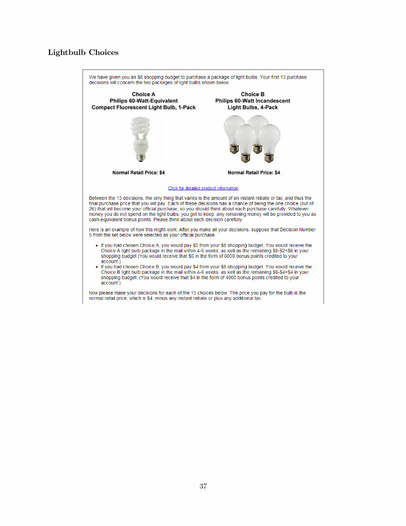
Lightbulb Choices

37

Detailed Product Information Screen

38

Baseline Lightbulb Choice Screen

Note: This does not show all of the 13 Decision Numbers.

39

Balanced Treatment Introductory Screen

40

Total Cost Information Screen

41

Disposal and Warm-Up Information Screen

42

Control Introductory Screen

43

Number of Bulbs by Sector Information Screen

44

Sales Trends Information Screen

45

Endline Choice Screen

Note: This does not show all of the 13 Decision Numbers.

46

Post-Experiment Survey Questions

Question 1. How important were the following factors in your purchase decision? [Rate from 1-10]

1. Energy use

2. Time required for the bulb to reach full brightness after it is turned on

3. Bulb lifetime

4. Mercury content and protocols for proper disposal

Question 2. Do you think that the intent of the study was to . . . [Multiple responses allowed]

1. Understand the e¤ect of rebates and taxes on purchasing patterns

2. Understand why people buy incandescents vs. CFLs

3. Test whether the number of bulbs in a package a¤ects purchasing patterns

4. Test di¤erent ways to educate people about light bulbs

5. Persuade people to buy incandescents

6. Persuade people to buy CFLs

7. Predict the future popularity of incandescents vs. CFLs

8. None of the above

[For consumers who selected "Persuade people to buy incandescents" or "Persuade people to buy CFLs"]If you thought that the survey was trying to persuade you to buy an incandescent or CFL, did this a¤ect yourpurchase decisions?

� No.

� Yes. This made me more likely to purchase the incandescent.

� Yes. This made me more likely to purchase the CFL.

Question 3. Part A: The typical CFL lasts 8000 hours, or about eight years at typical usage rates. Doyou think it costs more or less to buy electricity for that 8000 hours of light from compact �uorescent lightbulbs (CFLs) compared to incandescent light bulbs?

� More

� Less

Part B: At national average electricity prices, how much [more/less] does it cost to buy electricity forthat 8000 hours of light from compact �uorescent light bulbs (CFLs) compared to incandescent light bulbs?Just give your best guess.

47

Question 4. Some states and local areas have rebates, low-interest loans, or other incentives available forenergy e¢ ciency. These might include rebates for Energy Star appliances or energy e¢ cient light bulbs, low-interest loans for energy-saving home improvements, government-funded weatherization, and other programs.Are any such programs available in your area?

1. Yes

2. I think so, but I�m not sure

3. I�m not sure at all

4. I think not, but I�m not sure

5. No

48

Question 5. This question is about hypothetical choices and does not a¤ect your earnings in this study.Suppose that you could get the amount under �Option A�(i.e. $100), or the amount under �Option B�

a year later. Assume it�s no more work for you to receive the money under Option A than under Option B,and that you would receive the money for sure, regardless of when you choose to receive it. Which would youprefer?

Notes: This does not show all of the 18 choices. Participants were randomly assigned to receive eitherthis table or another table that was identical except that the bottom half and top half were switched, sothat the one year vs. two year tradeo¤s were presented �rst.

49

Appendix 4: Additional Results from the TESS Experiment

Table A4-1: Treatment E¤ects Conditional on Perceived Intent of Study

(1) (2) (3)Base

1(Treatment) 1.123 0.852 0.791

(0.341)*** (0.423)** (0.424)*

N 1,105 1,103 1,102

Other Individual Characteristics Yes Yes Yes

Perceived Intent Indicators No Yes Yes

Self-Reported Changed Purchase Indicators No No Yes

Notes: Column 1 replicates estimates of Equation (9) from column 2 of Table 4. Columns 2 and 3include indicator variables for each consumer�s perceived intent of the study, as summarized in the top panelof Table 5. Column 3 further adds indicators for whether the consumer reported that the experiment changedpurchasing decisions, as summarized in the bottom panel of Table 5. Robust standard errors in parenthesis.*, **, ***: Statistically signi�cant with 90, 95, and 99 percent con�dence, respectively. Observations areweighted for national representativeness.

Table A4-2: E¤ects on Important Factors in Purchase Decision

(1) (2) (3) (4)Energy Bulb Warm-Up Mercury andUse Lifetime Time Disposal

1(Balanced Treatment) 0.459 0.516 -1.033 -0.032

(0.181)** (0.167)*** (0.200)*** (0.211)

1(Positive Treatment) 0.619 0.595 -0.095 0.055

(0.176)*** (0.161)*** (0.197) (0.205)

Constant 7.237 7.516 5.282 5.916

(0.129)*** (0.117)*** (0.138)*** (0.144)***

N 1,214 1,236 1,233 1,242

Notes: This table reports treatment e¤ects on self-reported importance of di¤erent factors in purchasedecisions. Robust standard errors in parenthesis. *, **, ***: Statistically signi�cant with 90, 95, and 99percent con�dence, respectively. Observations are weighted for national representativeness.

50

Table A4-3: Association of Present Bias with CFL Demand

(1) (2) (3) (4)

� 0.081 0.255 0.235

(0.369) (0.396) (0.404)

� 0.584 0.531 0.459

(0.412) (0.401) (0.379)

1(� < 1) -0.007

(0.354)

N 1,105 1,105 1,095 1,095

Individual Characteristics No No Yes Yes

Notes: Left-hand-side variable is baseline relative WTP for the CFL v0. � and � re�ect parametersof the quasi-hyperbolic model from hypothetical intertemporal tradeo¤s, as described in the body of thepaper. Robust standard errors in parenthesis. *, **, ***: Statistically signi�cant with 90, 95, and 99 percentcon�dence, respectively. Observations are weighted for national representativeness.

51