the latent relation mapping engine: algorithm and experimentscogprints.org/6305/1/nrc-50738.pdf ·...

Journal of Artificial Intelligence Research 33 (2008) 615-655 Submitted 09/08; published 12/08

The Latent Relation Mapping Engine:Algorithm and Experiments

Peter D. Turney [email protected]

Institute for Information TechnologyNational Research Council CanadaOttawa, Ontario, Canada, K1A 0R6

Abstract

Many AI researchers and cognitive scientists have argued that analogy is the coreof cognition. The most influential work on computational modeling of analogy-making isStructure Mapping Theory (SMT) and its implementation in the Structure Mapping Engine(SME). A limitation of SME is the requirement for complex hand-coded representations.We introduce the Latent Relation Mapping Engine (LRME), which combines ideas fromSME and Latent Relational Analysis (LRA) in order to remove the requirement for hand-coded representations. LRME builds analogical mappings between lists of words, using alarge corpus of raw text to automatically discover the semantic relations among the words.We evaluate LRME on a set of twenty analogical mapping problems, ten based on scientificanalogies and ten based on common metaphors. LRME achieves human-level performanceon the twenty problems. We compare LRME with a variety of alternative approaches andfind that they are not able to reach the same level of performance.

1. Introduction

When we are faced with a problem, we try to recall similar problems that we have facedin the past, so that we can transfer our knowledge from past experience to the currentproblem. We make an analogy between the past situation and the current situation, and weuse the analogy to transfer knowledge (Gentner, 1983; Minsky, 1986; Holyoak & Thagard,1995; Hofstadter, 2001; Hawkins & Blakeslee, 2004).

In his survey of the computational modeling of analogy-making, French (2002) citesStructure Mapping Theory (SMT) (Gentner, 1983) and its implementation in the StructureMapping Engine (SME) (Falkenhainer, Forbus, & Gentner, 1989) as the most influentialwork on modeling of analogy-making. In SME, an analogical mapping M : A → B is froma source A to a target B. The source is more familiar, more known, or more concrete,whereas the target is relatively unfamiliar, unknown, or abstract. The analogical mappingis used to transfer knowledge from the source to the target.

Gentner (1983) argues that there are two kinds of similarity, attributional similarityand relational similarity. The distinction between attributes and relations may be under-stood in terms of predicate logic. An attribute is a predicate with one argument, such aslarge(X), meaning X is large. A relation is a predicate with two or more arguments, suchas collides with(X, Y ), meaning X collides with Y .

The Structure Mapping Engine prefers mappings based on relational similarity overmappings based on attributional similarity (Falkenhainer et al., 1989). For example, SMEis able to build a mapping from a representation of the solar system (the source) to a

c©2008 National Research Council Canada. Reprinted with permission.

Turney

representation of the Rutherford-Bohr model of the atom (the target). The sun is mappedto the nucleus, planets are mapped to electrons, and mass is mapped to charge. Note thatthis mapping emphasizes relational similarity. The sun and the nucleus are very differentin terms of their attributes: the sun is very large and the nucleus is very small. Likewise,planets and electrons have little attributional similarity. On the other hand, planets revolvearound the sun like electrons revolve around the nucleus. The mass of the sun attracts themass of the planets like the charge of the nucleus attracts the charge of the electrons.

Gentner (1991) provides evidence that children rely primarily on attributional similarityfor mapping, gradually switching over to relational similarity as they mature. She uses theterms mere appearance to refer to mapping based mostly on attributional similarity, analogyto refer to mapping based mostly on relational similarity, and literal similarity to refer to amixture of attributional and relational similarity. Since we use analogical mappings to solveproblems and make predictions, we should focus on structure, especially causal relations,and look beyond the surface attributes of things (Gentner, 1983). The analogy betweenthe solar system and the Rutherford-Bohr model of the atom illustrates the importance ofgoing beyond mere appearance, to the underlying structures.

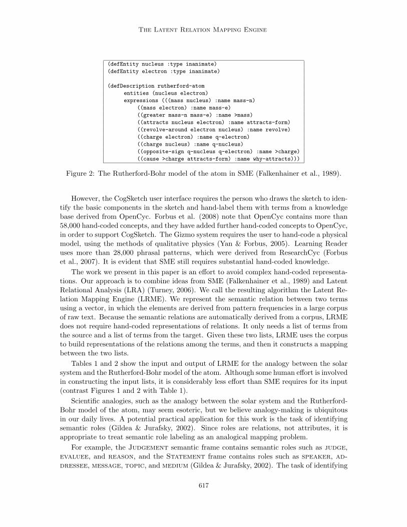
Figures 1 and 2 show the LISP representations used by SME as input for the analogybetween the solar system and the atom (Falkenhainer et al., 1989). Chalmers, French,and Hofstadter (1992) criticize SME’s requirement for complex hand-coded representations.They argue that most of the hard work is done by the human who creates these high-levelhand-coded representations, rather than by SME.

(defEntity sun :type inanimate)

(defEntity planet :type inanimate)

(defDescription solar-system

entities (sun planet)

expressions (((mass sun) :name mass-sun)

((mass planet) :name mass-planet)

((greater mass-sun mass-planet) :name >mass)

((attracts sun planet) :name attracts-form)

((revolve-around planet sun) :name revolve)

((and >mass attracts-form) :name and1)

((cause and1 revolve) :name cause-revolve)

((temperature sun) :name temp-sun)

((temperature planet) :name temp-planet)

((greater temp-sun temp-planet) :name >temp)

((gravity mass-sun mass-planet) :name force-gravity)

((cause force-gravity attracts-form) :name why-attracts)))

Figure 1: The representation of the solar system in SME (Falkenhainer et al., 1989).

Gentner, Forbus, and their colleagues have attempted to avoid hand-coding in theirrecent work with SME.1 The CogSketch system can generate LISP representations fromsimple sketches (Forbus, Usher, Lovett, Lockwood, & Wetzel, 2008). The Gizmo systemcan generate LISP representations from qualitative physics models (Yan & Forbus, 2005).The Learning Reader system can generate LISP representations from natural language text(Forbus et al., 2007). These systems do not require LISP input.

1. Dedre Gentner, personal communication, October 29, 2008.

616

The Latent Relation Mapping Engine

(defEntity nucleus :type inanimate)

(defEntity electron :type inanimate)

(defDescription rutherford-atom

entities (nucleus electron)

expressions (((mass nucleus) :name mass-n)

((mass electron) :name mass-e)

((greater mass-n mass-e) :name >mass)

((attracts nucleus electron) :name attracts-form)

((revolve-around electron nucleus) :name revolve)

((charge electron) :name q-electron)

((charge nucleus) :name q-nucleus)

((opposite-sign q-nucleus q-electron) :name >charge)

((cause >charge attracts-form) :name why-attracts)))

Figure 2: The Rutherford-Bohr model of the atom in SME (Falkenhainer et al., 1989).

However, the CogSketch user interface requires the person who draws the sketch to iden-tify the basic components in the sketch and hand-label them with terms from a knowledgebase derived from OpenCyc. Forbus et al. (2008) note that OpenCyc contains more than58,000 hand-coded concepts, and they have added further hand-coded concepts to OpenCyc,in order to support CogSketch. The Gizmo system requires the user to hand-code a physicalmodel, using the methods of qualitative physics (Yan & Forbus, 2005). Learning Readeruses more than 28,000 phrasal patterns, which were derived from ResearchCyc (Forbuset al., 2007). It is evident that SME still requires substantial hand-coded knowledge.

The work we present in this paper is an effort to avoid complex hand-coded representa-tions. Our approach is to combine ideas from SME (Falkenhainer et al., 1989) and LatentRelational Analysis (LRA) (Turney, 2006). We call the resulting algorithm the Latent Re-lation Mapping Engine (LRME). We represent the semantic relation between two termsusing a vector, in which the elements are derived from pattern frequencies in a large corpusof raw text. Because the semantic relations are automatically derived from a corpus, LRMEdoes not require hand-coded representations of relations. It only needs a list of terms fromthe source and a list of terms from the target. Given these two lists, LRME uses the corpusto build representations of the relations among the terms, and then it constructs a mappingbetween the two lists.

Tables 1 and 2 show the input and output of LRME for the analogy between the solarsystem and the Rutherford-Bohr model of the atom. Although some human effort is involvedin constructing the input lists, it is considerably less effort than SME requires for its input(contrast Figures 1 and 2 with Table 1).

Scientific analogies, such as the analogy between the solar system and the Rutherford-Bohr model of the atom, may seem esoteric, but we believe analogy-making is ubiquitousin our daily lives. A potential practical application for this work is the task of identifyingsemantic roles (Gildea & Jurafsky, 2002). Since roles are relations, not attributes, it isappropriate to treat semantic role labeling as an analogical mapping problem.

For example, the Judgement semantic frame contains semantic roles such as judge,evaluee, and reason, and the Statement frame contains roles such as speaker, ad-dressee, message, topic, and medium (Gildea & Jurafsky, 2002). The task of identifying

617

Turney

Source A

planetattractsrevolvessungravitysolar systemmass

Target B

revolvesatomattractselectromagnetismnucleuschargeelectron

Table 1: The representation of the input in LRME.

Source A Mapping M Target B

solar system → atomsun → nucleusplanet → electronmass → chargeattracts → attractsrevolves → revolvesgravity → electromagnetism

Table 2: The representation of the output in LRME.

semantic roles is to automatically label sentences with their roles, as in the following exam-ples (Gildea & Jurafsky, 2002):

• [Judge She] blames [Evaluee the Government] [Reason for failing to do enough tohelp].

• [Speaker We] talked [Topic about the proposal] [Medium over the phone].

If we have a training set of labeled sentences and a testing set of unlabeled sentences, thenwe may view the task of labeling the testing sentences as a problem of creating analogicalmappings between the training sentences (sources) and the testing sentences (targets). Ta-ble 3 shows how “She blames the Government for failing to do enough to help.” might bemapped to “They blame the company for polluting the environment.” Once a mapping hasbeen found, we can transfer knowledge, in the form of semantic role labels, from the sourceto the target.

Source A Mapping M Target B

she → theyblames → blamegovernment → companyfailing → pollutinghelp → environment

Table 3: Semantic role labeling as analogical mapping.

In Section 2, we briefly discuss the hypotheses behind the design of LRME. We thenprecisely define the task that is performed by LRME, a specific form of analogical mapping,

618


in Section 3. LRME builds on Latent Relational Analysis (LRA), hence we summarize LRAin Section 4. We discuss potential applications of LRME in Section 5.

To evaluate LRME, we created twenty analogical mapping problems, ten science anal-ogy problems (Holyoak & Thagard, 1995) and ten common metaphor problems (Lakoff &Johnson, 1980). Table 1 is one of the science analogy problems. Our intended solution isgiven in Table 2. To validate our intended solutions, we gave our colleagues the lists ofterms (as in Table 1) and asked them to generate mappings between the lists. Section 6presents the results of this experiment. Across the twenty problems, the average agreementwith our intended solutions (as in Table 2) was 87.6%.

The LRME algorithm is outlined in Section 7, along with its evaluation on the twentymapping problems. LRME achieves an accuracy of 91.5%. The difference between thisperformance and the human average of 87.6% is not statistically significant.

Section 8 examines a variety of alternative approaches to the analogy mapping task. Thebest approach achieves an accuracy of 76.8%, but this approach requires hand-coded part-of-speech tags. This performance is significantly below LRME and human performance.

In Section 9, we discuss some questions that are raised by the results in the precedingsections. Related work is described in Section 10, future work and limitations are consideredin Section 11, and we conclude in Section 12.

2. Guiding Hypotheses

In this section, we list some of the assumptions that have guided the design of LRME. Theresults we present in this paper do not necessarily require these assumptions, but it mightbe helpful to the reader, to understand the reasoning behind our approach.

1. Analogies and semantic relations: Analogies are based on semantic relations(Gentner, 1983). For example, the analogy between the solar system and the Ruther-ford-Bohr model of the atom is based on the similarity of the semantic relationsamong the concepts involved in our understanding of the solar system to the semanticrelations among the concepts involved in the Rutherford-Bohr model of the atom.

2. Co-occurrences and semantic relations: Two terms have an interesting, signif-icant semantic relation if and only if they they tend to co-occur within a relativelysmall window (e.g., five words) in a relatively large corpus (e.g., 1010 words). Havingan interesting semantic relation causes co-occurrence and co-occurrence is a reliableindicator of an interesting semantic relation (Firth, 1957).

3. Meanings and semantic relations: Meaning has more to do with relations amongwords than individual words. Individual words tend to be ambiguous and polysemous.By putting two words into a pair, we constrain their possible meanings. By puttingwords into a sentence, with multiple relations among the words in the sentence, weconstrain the possible meanings further. If we focus on word pairs (or tuples), insteadof individual words, word sense disambiguation is less problematic. Perhaps a wordhas no sense apart from its relations with other words (Kilgarriff, 1997).

4. Pattern distributions and semantic relations: There is a many-to-many map-ping between semantic relations and the patterns in which two terms co-occur. Forexample, the relation CauseEffect(X,Y ) may be expressed as “X causes Y ”, “Y

619

Turney

from X”, “Y due to X”, “Y because of X”, and so on. Likewise, the pattern“Y from X” may be an expression of CauseEffect(X, Y ) (“sick from bacteria”) orOriginEntity(X, Y ) (“oranges from Spain”). However, for a given X and Y , the sta-tistical distribution of patterns in which X and Y co-occur is a reliable signature ofthe semantic relations between X and Y (Turney, 2006).

To the extent that LRME works, we believe its success lends some support to these hy-potheses.

3. The Task

In this paper, we examine algorithms that generate analogical mappings. For simplicity, werestrict the task to generating bijective mappings; that is, mappings that are both injective(one-to-one; there is no instance in which two terms in the source map to the same termin the target) and surjective (onto; the source terms cover all of the target terms; there isno target term that is left out of the mapping). We assume that the entities that are to bemapped are given as input. Formally, the input I for the algorithms is two sets of terms, Aand B.

I = {〈A, B〉} (1)

Since the mappings are bijective, A and B must contain the same number of terms, m.

A = {a1, a2, . . . , am} (2)B = {b1, b2, . . . , bm} (3)

A term, ai or bj , may consist of a single word (planet) or a compound of two or more words(solar system). The words may be any part of speech (nouns, verbs, adjectives, or adverbs).The output O is a bijective mapping M from A to B.

O = {M : A → B} (4)M(ai) ∈ B (5)M(A) = {M(a1), M(a2), . . . ,M(am)} = B (6)

The algorithms that we consider here can accept a batch of multiple independent mappingproblems as input and generate a mapping for each one as output.

I = {〈A1, B1〉 , 〈A2, B2〉 , . . . , 〈An, Bn〉} (7)O = {M1 : A1 → B1, M2 : A2 → B2, . . . ,Mn : An → Bn} (8)

Suppose the terms in A are in some arbitrary order a.

a = 〈a1, a2, . . . , am〉 (9)

The mapping function M : A → B, given a, determines a unique ordering b of B.

620


b = 〈M(a1), M(a2), . . . ,M(am)〉 (10)

Likewise, an ordering b of B, given a, defines a unique mapping function M . Since thereare m! possible orderings of B, there are also m! possible mappings from A to B. The taskis to search through the m! mappings and find the best one. (Section 6 shows that there isa relatively high degree of consensus about which mappings are best.)

Let P (A, B) be the set of all m! bijective mappings from A to B. (P stands for permu-tation, since each mapping corresponds to a permutation.)

P (A, B) = {M1, M2, . . . ,Mm!} (11)m = |A| = |B| (12)m! = |P (A, B)| (13)

In the following experiments, m is 7 on average and 9 at most, so m! is usually around7! = 5, 040 and at most 9! = 362, 880. It is feasible for us to exhaustively search P (A, B).

We explore two basic kinds of algorithms for generating analogical mappings, algorithmsbased on attributional similarity and algorithms based on relational similarity (Turney,2006). The attributional similarity between two words, sima(a, b) ∈ <, depends on thedegree of correspondence between the properties of a and b. The more correspondencethere is, the greater their attributional similarity. The relational similarity between twopairs of words, simr(a : b, c : d) ∈ <, depends on the degree of correspondence between therelations of a : b and c : d. The more correspondence there is, the greater their relationalsimilarity. For example, dog and wolf have a relatively high degree of attributional similarity,whereas dog : bark and cat :meow have a relatively high degree of relational similarity.

Attributional mapping algorithms seek the mapping (or mappings) Ma that maximizesthe sum of the attributional similarities between the terms in A and the correspondingterms in B. (When there are multiple mappings that maximize the sum, we break the tieby randomly choosing one of them.)

Ma = arg maxM∈P (A,B)

m∑i=1

sima(ai, M(ai)) (14)

Relational mapping algorithms seek the mapping (or mappings) Mr that maximizes thesum of the relational similarities.

Mr = arg maxM∈P (A,B)

m∑i=1

m∑j=i+1

simr(ai :aj , M(ai) :M(aj)) (15)

In (15), we assume that simr is symmetrical. For example, the degree of relational similaritybetween dog : bark and cat :meow is the same as the degree of relational similarity betweenbark : dog and meow : cat.

simr(a :b, c :d) = simr(b :a, d :c) (16)

We also assume that simr(a :a, b :b) is not interesting; for example, it may be some constantvalue for all a and b. Therefore (15) is designed so that i is always less than j.

621

Turney

Let scorer(M) and scorea(M) be defined as follows.

scorer(M) =m∑

i=1

m∑j=i+1


scorea(M) =m∑

i=1


Now Mr and Ma may be defined in terms of scorer(M) and scorea(M).


scorer(M) (19)


scorea(M) (20)

Mr is the best mapping according to simr and Ma is the best mapping according to sima.Recall Gentner’s (1991) terms, discussed in Section 1, mere appearance (mostly attribu-

tional similarity), analogy (mostly relational similarity), and literal similarity (a mixture ofattributional and relational similarity). We take it that Mr is an abstract model of map-ping based on analogy and Ma is a model of mere appearance. For literal similarity, we cancombine Mr and Ma, but we should take care to normalize scorer(M) and scorea(M) beforewe combine them. (We experiment with combining them in Section 9.2.)

4. Latent Relational Analysis

LRME uses a simplified form of Latent Relational Analysis (LRA) (Turney, 2005, 2006)to calculate the relational similarity between pairs of words. We will briefly describe pastwork with LRA before we present LRME.

LRA takes as input I a set of word pairs and generates as output O the relationalsimilarity simr(ai :bi, aj :bj) between any two pairs in the input.

I = {a1 :b1, a2 :b2, . . . , an :bn} (21)O = {simr : I × I → <} (22)

LRA was designed to evaluate proportional analogies. Proportional analogies have the forma :b ::c :d, which means “a is to b as c is to d”. For example, mason : stone :: carpenter :woodmeans “mason is to stone as carpenter is to wood”. A mason is an artisan who works withstone and a carpenter is an artisan who works with wood.

We consider proportional analogies to be a special case of bijective analogical mapping,as defined in Section 3, in which |A| = |B| = m = 2. For example, a1 :a2 ::b1 :b2 is equivalentto M0 in (23).

A = {a1, a2} , B = {b1, b2} , M0(a1) = b1, M0(a2) = b2. (23)

From the definition of scorer(M) in (17), we have the following result for M0.

622


scorer(M0) = simr(a1 :a2, M0(a1) :M0(a2)) = simr(a1 :a2, b1 :b2) (24)

That is, the quality of the proportional analogy mason : stone :: carpenter :wood is given bysimr(mason :stone, carpenter :wood).

Proportional analogies may also be evaluated using attributional similarity. From thedefinition of scorea(M) in (18), we have the following result for M0.

scorea(M0) = sima(a1, M0(a1)) + sima(a2, M0(a2)) = sima(a1, b1) + sima(a2, b2) (25)

For attributional similarity, the quality of the proportional analogy mason : stone :: carpenter :wood is given by sima(mason, carpenter) + sima(stone, wood).

LRA only handles proportional analogies. The main contribution of LRME is to extendLRA beyond proportional analogies to bijective analogies for which m > 2.

Turney (2006) describes ten potential applications of LRA: recognizing proportionalanalogies, structure mapping theory, modeling metaphor, classifying semantic relations,word sense disambiguation, information extraction, question answering, automatic the-saurus generation, information retrieval, and identifying semantic roles. Two of theseapplications (evaluating proportional analogies and classifying semantic relations) are ex-perimentally evaluated, with state-of-the-art results.

Turney (2006) compares the performance of relational similarity (24) and attributionalsimilarity (25) on the task of solving 374 multiple-choice proportional analogy questions fromthe SAT college entrance test. LRA is used to measure relational similarity and a varietyof lexicon-based and corpus-based algorithms are used to measure attributional similarity.LRA achieves an accuracy of 56% on the 374 SAT questions, which is not significantlydifferent from the average human score of 57%. On the other hand, the best performanceby attributional similarity is 35%. The results show that attributional similarity is betterthan random guessing, but not as good as relational similarity. This result is consistentwith Gentner’s (1991) theory of the maturation of human similarity judgments.

Turney (2006) also applies LRA to the task of classifying semantic relations in noun-modifier expressions. A noun-modifier expression is a phrase, such as laser printer, in whichthe head noun (printer) is preceded by a modifier (laser). The task is to identify the semanticrelation between the noun and the modifier. In this case, the relation is instrument; thelaser is an instrument used by the printer. On a set of 600 hand-labeled noun-modifier pairswith five different classes of semantic relations, LRA attains 58% accuracy.

Turney (2008) employs a variation of LRA for solving four different language tests,achieving 52% accuracy on SAT analogy questions, 76% accuracy on TOEFL synonymquestions, 75% accuracy on the task of distinguishing synonyms from antonyms, and 77%accuracy on the task of distinguishing words that are similar, words that are associated,and words that are both similar and associated. The same core algorithm is used for allfour tests, with no tuning of the parameters to the particular test.

5. Applications for LRME

Since LRME is an extension of LRA, every potential application of LRA is also a potentialapplication of LRME. The advantage of LRME over LRA is the ability to handle bijective

623

Turney

analogies when m > 2 (where m = |A| = |B|). In this section, we consider the kinds ofapplications that might benefit from this ability.

In Section 7.2, we evaluate LRME on science analogies and common metaphors, whichsupports the claim that these two applications benefit from the ability to handle larger setsof terms. In Section 1, we saw that identifying semantic roles (Gildea & Jurafsky, 2002)also involves more than two terms, and we believe that LRME will be superior to LRA forsemantic role labeling.

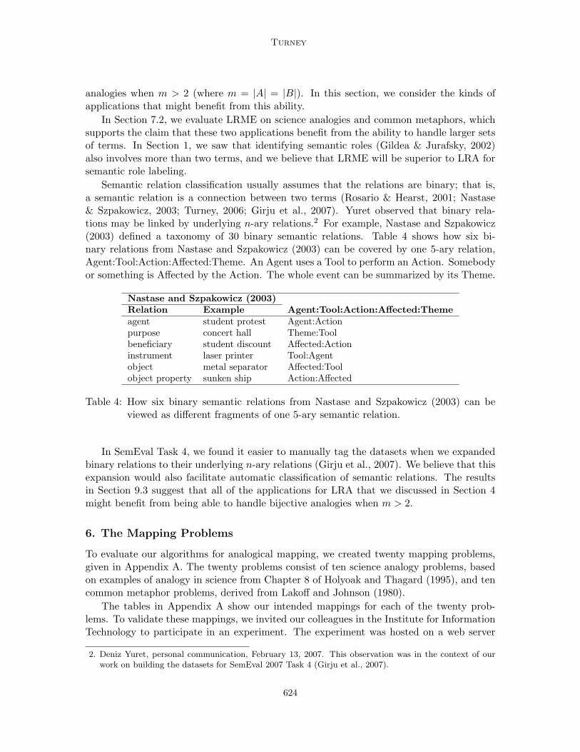
Semantic relation classification usually assumes that the relations are binary; that is,a semantic relation is a connection between two terms (Rosario & Hearst, 2001; Nastase& Szpakowicz, 2003; Turney, 2006; Girju et al., 2007). Yuret observed that binary rela-tions may be linked by underlying n-ary relations.2 For example, Nastase and Szpakowicz(2003) defined a taxonomy of 30 binary semantic relations. Table 4 shows how six bi-nary relations from Nastase and Szpakowicz (2003) can be covered by one 5-ary relation,Agent:Tool:Action:Affected:Theme. An Agent uses a Tool to perform an Action. Somebodyor something is Affected by the Action. The whole event can be summarized by its Theme.

Nastase and Szpakowicz (2003)Relation Example Agent:Tool:Action:Affected:Themeagent student protest Agent:Actionpurpose concert hall Theme:Toolbeneficiary student discount Affected:Actioninstrument laser printer Tool:Agentobject metal separator Affected:Toolobject property sunken ship Action:Affected

Table 4: How six binary semantic relations from Nastase and Szpakowicz (2003) can beviewed as different fragments of one 5-ary semantic relation.

In SemEval Task 4, we found it easier to manually tag the datasets when we expandedbinary relations to their underlying n-ary relations (Girju et al., 2007). We believe that thisexpansion would also facilitate automatic classification of semantic relations. The resultsin Section 9.3 suggest that all of the applications for LRA that we discussed in Section 4might benefit from being able to handle bijective analogies when m > 2.

6. The Mapping Problems

To evaluate our algorithms for analogical mapping, we created twenty mapping problems,given in Appendix A. The twenty problems consist of ten science analogy problems, basedon examples of analogy in science from Chapter 8 of Holyoak and Thagard (1995), and tencommon metaphor problems, derived from Lakoff and Johnson (1980).

The tables in Appendix A show our intended mappings for each of the twenty prob-lems. To validate these mappings, we invited our colleagues in the Institute for InformationTechnology to participate in an experiment. The experiment was hosted on a web server

2. Deniz Yuret, personal communication, February 13, 2007. This observation was in the context of ourwork on building the datasets for SemEval 2007 Task 4 (Girju et al., 2007).

624


(only accessible inside our institute) and people participated anonymously, using their webbrowsers in their offices. There were 39 volunteers who began the experiment and 22 whowent all the way to the end. In our analysis, we use only the data from the 22 participantswho completed all of the mapping problems.

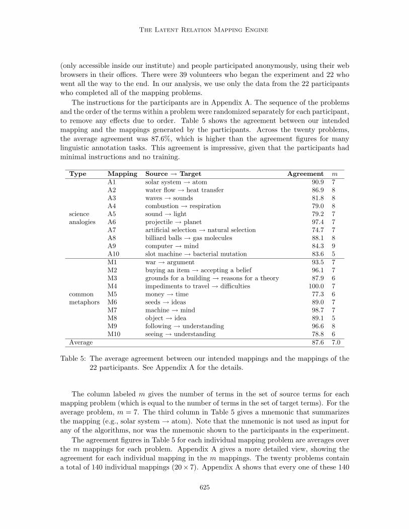
The instructions for the participants are in Appendix A. The sequence of the problemsand the order of the terms within a problem were randomized separately for each participant,to remove any effects due to order. Table 5 shows the agreement between our intendedmapping and the mappings generated by the participants. Across the twenty problems,the average agreement was 87.6%, which is higher than the agreement figures for manylinguistic annotation tasks. This agreement is impressive, given that the participants hadminimal instructions and no training.

Type Mapping Source → Target Agreement mA1 solar system → atom 90.9 7A2 water flow → heat transfer 86.9 8A3 waves → sounds 81.8 8A4 combustion → respiration 79.0 8

science A5 sound → light 79.2 7analogies A6 projectile → planet 97.4 7

A7 artificial selection → natural selection 74.7 7A8 billiard balls → gas molecules 88.1 8A9 computer → mind 84.3 9A10 slot machine → bacterial mutation 83.6 5M1 war → argument 93.5 7M2 buying an item → accepting a belief 96.1 7M3 grounds for a building → reasons for a theory 87.9 6M4 impediments to travel → difficulties 100.0 7

common M5 money → time 77.3 6metaphors M6 seeds → ideas 89.0 7

M7 machine → mind 98.7 7M8 object → idea 89.1 5M9 following → understanding 96.6 8M10 seeing → understanding 78.8 6

Average 87.6 7.0

Table 5: The average agreement between our intended mappings and the mappings of the22 participants. See Appendix A for the details.

The column labeled m gives the number of terms in the set of source terms for eachmapping problem (which is equal to the number of terms in the set of target terms). For theaverage problem, m = 7. The third column in Table 5 gives a mnemonic that summarizesthe mapping (e.g., solar system → atom). Note that the mnemonic is not used as input forany of the algorithms, nor was the mnemonic shown to the participants in the experiment.

The agreement figures in Table 5 for each individual mapping problem are averages overthe m mappings for each problem. Appendix A gives a more detailed view, showing theagreement for each individual mapping in the m mappings. The twenty problems containa total of 140 individual mappings (20× 7). Appendix A shows that every one of these 140

625

Turney

mappings has an agreement of 50% or higher. That is, in every case, the majority of theparticipants agreed with our intended mapping. (There are two cases where the agreementis exactly 50%. See problems A5 in Table 14 and M5 in Table 16 in Appendix A.)

If we select the mapping that is chosen by the majority of the 22 participants, then wewill get a perfect score on all twenty problems. More precisely, if we try all m! mappings foreach problem, and select the mapping that maximizes the sum of the number of participantswho agree with each individual mapping in the m mappings, then we will have a score of100% on all twenty problems. This is strong support for the intended mappings that aregiven in Appendix A.

In Section 3, we applied Genter’s (1991) categories – mere appearance (mostly attribu-tional similarity), analogy (mostly relational similarity), and literal similarity (a mixtureof attributional and relational similarity) – to the mappings Mr and Ma, where Mr is thebest mapping according to simr and Ma is the best mapping according to sima. The twentymapping problems were chosen as analogy problems; that is, the intended mappings inAppendix A are meant to be relational mappings, Mr; mappings that maximize relationalsimilarity, simr. We have tried to avoid mere appearance and literal similarity.

In Section 7 we use the twenty mapping problems to evaluate a relational mappingalgorithm (LRME), and in Section 8 we use them to evaluate several different attributionalmapping algorithms. Our hypothesis is that LRME will perform significantly better thanany of the attributional mapping algorithms on the twenty mapping problems, because theyare analogy problems (not mere appearance problems and not literal similarity problems).We expect relational and attributional mapping algorithms would perform approximatelyequally well on literal similarity problems, and we expect that mere appearance problemswould favour attributional algorithms over relational algorithms, but we do not test theselatter two hypotheses, because our primary interest in this paper is analogy-making.

Our goal is to test the hypothesis that there is a real, practical, effective, measurabledifference between the output of LRME and the output of the various attributional map-ping algorithms. A skeptic might claim that relational similarity simr(a : b, c : d) can bereduced to attributional similarity sima(a, c) + sima(b, d); therefore our relational mappingalgorithm is a complicated solution to an illusory problem. A slightly less skeptical claimis that relational similarity versus attributional similarity is a valid distinction in cognitivepsychology, but our relational mapping algorithm does not capture this distinction. To testour hypothesis and refute these skeptical claims, we have created twenty analogical mappingproblems, and we will show that LRME handles these problems significantly better thanthe various attributional mapping algorithms.

7. The Latent Relation Mapping Engine

The Latent Relation Mapping Engine (LRME) seeks the mapping Mr that maximizes thesum of the relational similarities.


m∑i=1

m∑j=i+1


We search for Mr by exhaustively evaluating all of the possibilities. Ties are broken ran-domly. We use a simplified form of LRA (Turney, 2006) to calculate simr.

626


7.1 Algorithm

Briefly, the idea of LRME is to build a pair-pattern matrix X, in which the rows correspondto pairs of terms and the columns correspond to patterns. For example, the row xi: mightcorrespond to the pair of terms sun : solar system and the column x:j might correspond tothe pattern “∗ X centered Y ∗”. In these patterns, “∗” is a wild card, which can matchany single word. The value of an element xij in X is based on the frequency of the patternfor x:j , when X and Y are instantiated by the terms in the pair for xi:. For example, if wetake the pattern “∗ X centered Y ∗” and instantiate X : Y with the pair sun : solar system,then we have the pattern “∗ sun centered solar system ∗”, and thus the value of the elementxij is based on the frequency of “∗ sun centered solar system ∗” in the corpus. The matrixX is smoothed with a truncated singular value decomposition (SVD) (Golub & Van Loan,1996) and the relational similarity simr between two pairs of terms is given by the cosine ofthe angle between the two corresponding row vectors in X.

In more detail, LRME takes as input I a set of mapping problems and generates asoutput O a corresponding set of mappings.

I = {〈A1, B1〉 , 〈A2, B2〉 , . . . , 〈An, Bn〉} (27)O = {M1 : A1 → B1, M2 : A2 → B2, . . . ,Mn : An → Bn} (28)

In the following experiments, all twenty mapping problems (Appendix A) are processed inone batch (n = 20).

The first step is to make a list R that contains all pairs of terms in the input I. Foreach mapping problem 〈A, B〉 in I, we add to R all pairs ai : aj , such that ai and aj aremembers of A, i 6= j, and all pairs bi : bj , such that bi and bj are members of B, i 6= j.If |A| = |B| = m, then there are m(m − 1) pairs from A and m(m − 1) pairs from B.3 Atypical pair in R would be sun : solar system. We do not allow duplicates in R; R is a listof pair types, not pair tokens. For our twenty mapping problems, R is a list of 1,694 pairs.

For each pair r in R, we make a list S(r) of the phrases in the corpus that contain thepair r. Let ai : aj be the terms in the pair r. We search in the corpus for all phrases of thefollowing form:

“[0 to 1 words] ai [0 to 3 words] aj [0 to 1 words]” (29)

If ai : aj is in R, then aj : ai is also in R, so we find phrases with the members of the pairsin both orders, S(ai : aj) and S(aj : ai). The search template (29) is the same as used byTurney (2008).

In the following experiments, we search in a corpus of 5×1010 English words (about 280GB of plain text), consisting of web pages gathered by a web crawler.4 To retrieve phrases

3. We have m(m − 1) here, not m(m − 1)/2, because we need the pairs in both orders. We only wantto calculate simr for one order of the pairs, because i is always less than j in (26); however, to ensurethat simr is symmetrical, as in (16), we need to make the matrix X symmetrical, by having rows in thematrix for both orders of every pair.

4. The corpus was collected by Charles Clarke at the University of Waterloo. We can provide copies of thecorpus on request.

627

Turney

from the corpus, we use Wumpus (Buttcher & Clarke, 2005), an efficient search engine forpassage retrieval from large corpora.5

With the 1,694 pairs in R, we find a total of 1,996,464 phrases in the corpus, an averageof about 1,180 phrases per pair. For the pair r = sun : solar system, a typical phrase s inS(r) would be “a sun centered solar system illustrates”.

Next we make a list C of patterns, based on the phrases we have found. For each pairr in R, where r = ai : aj , if we found a phrase s in S(r), then we replace ai in s with Xand we replace aj with Y . The remaining words may be either left as they are or replacedwith a wild card symbol “∗”. We then replace ai in s with Y and aj with X, and replacethe remaining words with wild cards or leave them as they are. If there are n remainingwords in s, after ai and aj are replaced, then we generate 2n+1 patterns from s, and we addthese patterns to C. We only add new patterns to C; that is, C is a list of pattern types,not pattern tokens; there are no duplicates in C.

For example, for the pair sun : solar system, we found the phrase “a sun centered solarsystem illustrates”. When we replace ai : aj with X : Y , we have “a X centered Yillustrates”. There are three remaining words, so we can generate eight patterns, such as“a X ∗ Y illustrates”, “a X centered Y ∗”, “∗ X ∗ Y illustrates”, and so on. Each of thesepatterns is added to C. Then we replace ai : aj with Y : X, yielding “a Y centered Xillustrates”. This gives us another eight patterns, such as “a Y centered X ∗”. Thus thephrase “a sun centered solar system illustrates” generates a total of sixteen patterns, whichwe add to C.

Now we revise R, to make a list of pairs that will correspond to rows in the frequencymatrix F. We remove any pairs from R for which no phrases were found in the corpus,when the terms were in either order. Let ai : aj be the terms in the pair r. We remover from R if both S(ai : aj) and S(aj : ai) are empty. We remove such rows because theywould correspond to zero vectors in the matrix F. This reduces R from 1,694 pairs to 1,662pairs. Let nr be the number of pairs in R.

Next we revise C, to make a list of patterns that will correspond to columns in thefrequency matrix F. In the following experiments, at this stage, C contains millions ofpatterns, too many for efficient processing with a standard desktop computer. We need toreduce C to a more manageable size. We select the patterns that are shared by the mostpairs. Let c be a pattern in C. Let r be a pair in R. If there is a phrase s in S(r), suchthat there is a pattern generated from s that is identical to c, then we say that r is one ofthe pairs that generated c. We sort the patterns in C in descending order of the numberof pairs in R that generated each pattern, and we select the top tnr patterns from thissorted list. Following Turney (2008), we set the parameter t to 20; hence C is reduced tothe top 33,240 patterns (tnr = 20 × 1,662 = 33,240). Let nc be the number of patterns inC (nc = tnr).

Now that the rows R and columns C are defined, we can build the frequency matrixF. Let ri be the i-th pair of terms in R (e.g., let ri be sun : solar system) and let cj bethe j-th pattern in C (e.g., let cj be “∗ X centered Y ∗”). We instantiate X and Y in thepattern cj with the terms in ri (“∗ sun centered solar system ∗”). The element fij in F isthe frequency of this instantiated pattern in the corpus.

5. Wumpus was developed by Stefan Buttcher and it is available at http://www.wumpus-search.org/.

628


Note that we do not need to search again in the corpus for the instantiated pattern forfij , in order to find its frequency. In the process of creating each pattern, we can keep trackof how many phrases generated the pattern, for each pair. We can get the frequency for fij

by checking our record of the patterns that were generated by ri.The next step is to transform the matrix F of raw frequencies into a form X that

enhances the similarity measurement. Turney (2006) used the log entropy transformation,as suggested by Landauer and Dumais (1997). This is a kind of tf-idf (term frequencytimes inverse document frequency) transformation, which gives more weight to elements inthe matrix that are statistically surprising. However, Bullinaria and Levy (2007) recentlyachieved good results with a new transformation, called PPMIC (Positive Pointwise MutualInformation with Cosine); therefore LRME uses PPMIC. The raw frequencies in F are usedto calculate probabilities, from which we can calculate the pointwise mutual information(PMI) of each element in the matrix. Any element with a negative PMI is then set to zero.

pij =fij∑nr

i=1

∑ncj=1 fij

(30)

pi∗ =

∑ncj=1 fij∑nr

i=1

∑ncj=1 fij

(31)

p∗j =∑nr

i=1 fij∑nri=1

∑ncj=1 fij

(32)

pmiij = log(

pij

pi∗p∗j

)(33)

xij ={

pmiij if pmiij > 00 otherwise

(34)

Let ri be the i-th pair of terms in R (e.g., let ri be sun : solar system) and let cj be thej-th pattern in C (e.g., let cj be “∗X centered Y ∗”). In (33), pij is the estimated probabilityof the of the pattern cj instantiated with the pair ri (“∗ sun centered solar system ∗”), pi∗is the estimated probability of ri, and p∗j is the estimated probability of cj . If ri and cj arestatistically independent, then pi∗p∗j = pij (by the definition of independence), and thuspmiij is zero (since log(1) = 0). If there is an interesting semantic relation between theterms in ri, and the pattern cj captures an aspect of that semantic relation, then we shouldexpect pij to be larger than it would be if ri and cj were indepedent; hence we should findthat pij > pi∗p∗j , and thus pmiij is positive. (See Hypothesis 2 in Section 2.) On the otherhand, terms from completely different domains may avoid each other, in which case weshould find that pmiij is negative. PPMIC is designed to give a high value to xij when thepattern cj captures an aspect of the semantic relation between the terms in ri; otherwise,xij should have a value of zero, indicating that the pattern cj tells us nothing about thesemantic relation between the terms in ri.

In our experiments, F has a density of 4.6% (the percentage of nonzero elements) andX has a density of 3.8%. The lower density of X is due to elements with a negative PMI,which are transformed to zero by PPMIC.

629

Turney

Now we smooth X by applying a truncated singular value decomposition (SVD) (Golub& Van Loan, 1996). We use SVDLIBC to calculate the SVD of X.6 SVDLIBC is designedfor sparse (low density) matrices. SVD decomposes X into the product of three matricesUΣVT, where U and V are in column orthonormal form (i.e., the columns are orthogonaland have unit length, UTU = VTV = I) and Σ is a diagonal matrix of singular values(Golub & Van Loan, 1996). If X is of rank r, then Σ is also of rank r. Let Σk, wherek < r, be the diagonal matrix formed from the top k singular values, and let Uk and Vk bethe matrices produced by selecting the corresponding columns from U and V. The matrixUkΣkVT

k is the matrix of rank k that best approximates the original matrix X, in the sensethat it minimizes the approximation errors. That is, X = UkΣkVT

k minimizes ‖X−X‖F

over all matrices X of rank k, where ‖ . . . ‖F denotes the Frobenius norm (Golub & VanLoan, 1996). We may think of this matrix UkΣkVT

k as a smoothed or compressed versionof the original matrix X. Following Turney (2006), we set the parameter k to 300.

The relational similarity simr between two pairs in R is the inner product of the twocorresponding rows in UkΣkVT

k , after the rows have been normalized to unit length. We cansimplify calculations by dropping Vk (Deerwester, Dumais, Landauer, Furnas, & Harshman,1990). We take the matrix UkΣk and normalize each row to unit length. Let W be theresulting matrix. Now let Z be WWT, a square matrix of size nr×nr. This matrix containsthe cosines of all combinations of two pairs in R.

For a mapping problem 〈A, B〉 in I, let a : a′ be a pair of terms from A and let b : b′ bea pair of terms from B. Suppose that ri = a : a′ and rj = b : b′, where ri and rj are thei-th and j-th pairs in R. Then simr(a : a′, b : b′) = zij , where zij is the element in the i-throw and j-th column of Z. If either a : a′ or b : b′ is not in R, because S(a : a′), S(a′ : a),S(b : b′), or S(b′ : b) is empty, then we set the similarity to zero. Finally, for each mappingproblem in I, we output the map Mr that maximizes the sum of the relational similarities.


m∑i=1

m∑j=i+1


The simplified form of LRA used here to calculate simr differs from LRA used by Turney(2006) in several ways. In LRME, there is no use of synonyms to generate alternate forms ofthe pairs of terms. In LRME, there is no morphological processing of the terms. LRME usesPPMIC (Bullinaria & Levy, 2007) to process the raw frequencies, instead of log entropy.Following Turney (2008), LRME uses a slightly different search template (29) and LRMEsets the number of columns nc to tnr, instead of using a constant. In Section 7.2, weevaluate the impact of two of these changes (PPMIC and nc), but we have not testedthe other changes, which were mainly motivated by a desire for increased efficiency andsimplicity.

7.2 Experiments

We implemented LRME in Perl, making external calls to Wumpus for searching the corpusand to SVDLIBC for calculating SVD. We used the Perl Net::Telnet package for interprocess

6. SVDLIBC is the work of Doug Rohde and it is available at http://tedlab.mit.edu/∼dr/svdlibc/.

630


communication with Wumpus, the PDL (Perl Data Language) package for matrix manipu-lations (e.g., calculating cosines), and the List::Permutor package to generate permutations(i.e., to loop through P (A, B)).

We ran the following experiments on a dual core AMD Opteron 64 computer, running64 bit Linux. Most of the running time is spent searching the corpus for phrases. It took16 hours and 27 minutes for Wumpus to fetch the 1,996,464 phrases. The remaining stepstook 52 minutes, of which SVD took 10 minutes. The running time could be cut in half byusing RAID 0 to speed up disk access.

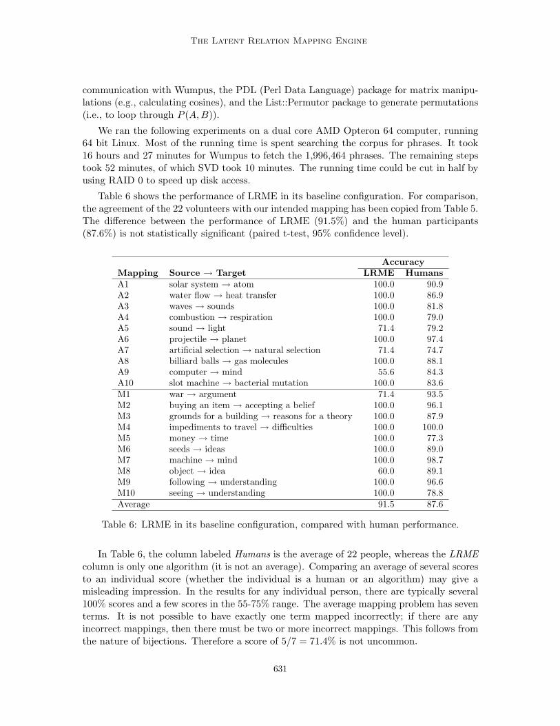
Table 6 shows the performance of LRME in its baseline configuration. For comparison,the agreement of the 22 volunteers with our intended mapping has been copied from Table 5.The difference between the performance of LRME (91.5%) and the human participants(87.6%) is not statistically significant (paired t-test, 95% confidence level).

AccuracyMapping Source → Target LRME HumansA1 solar system → atom 100.0 90.9A2 water flow → heat transfer 100.0 86.9A3 waves → sounds 100.0 81.8A4 combustion → respiration 100.0 79.0A5 sound → light 71.4 79.2A6 projectile → planet 100.0 97.4A7 artificial selection → natural selection 71.4 74.7A8 billiard balls → gas molecules 100.0 88.1A9 computer → mind 55.6 84.3A10 slot machine → bacterial mutation 100.0 83.6M1 war → argument 71.4 93.5M2 buying an item → accepting a belief 100.0 96.1M3 grounds for a building → reasons for a theory 100.0 87.9M4 impediments to travel → difficulties 100.0 100.0M5 money → time 100.0 77.3M6 seeds → ideas 100.0 89.0M7 machine → mind 100.0 98.7M8 object → idea 60.0 89.1M9 following → understanding 100.0 96.6M10 seeing → understanding 100.0 78.8Average 91.5 87.6

Table 6: LRME in its baseline configuration, compared with human performance.

In Table 6, the column labeled Humans is the average of 22 people, whereas the LRMEcolumn is only one algorithm (it is not an average). Comparing an average of several scoresto an individual score (whether the individual is a human or an algorithm) may give amisleading impression. In the results for any individual person, there are typically several100% scores and a few scores in the 55-75% range. The average mapping problem has seventerms. It is not possible to have exactly one term mapped incorrectly; if there are anyincorrect mappings, then there must be two or more incorrect mappings. This follows fromthe nature of bijections. Therefore a score of 5/7 = 71.4% is not uncommon.

631

Turney

Table 7 looks at the results from another perspective. The column labeled LRME wronggives the number of incorrect mappings made by LRME for each of the twenty problems.The five columns labeled Number of people with N wrong show, for various values of N ,how may of the 22 people made N incorrect mappings. For the average mapping problem,15 out of 22 participants had a perfect score (N = 0); of the remaining 7 participants, 5made only two mistakes (N = 2). Table 7 shows more clearly than Table 6 that LRME’sperformance is not significantly different from (individual) human performance. (For yetanother perspective, see Section 9.1).

LRME Number of people with N wrongMapping wrong N = 0 N = 1 N = 2 N = 3 N ≥ 4 mA1 0 16 0 4 2 0 7A2 0 14 0 5 0 3 8A3 0 9 0 9 2 2 8A4 0 9 0 9 0 4 8A5 2 10 0 7 2 3 7A6 0 20 0 2 0 0 7A7 2 8 0 6 6 2 7A8 0 13 0 8 0 1 8A9 4 11 0 7 2 2 9A10 0 13 0 9 0 0 5M1 2 17 0 5 0 0 7M2 0 19 0 3 0 0 7M3 0 14 0 8 0 0 6M4 0 22 0 0 0 0 7M5 0 9 0 11 0 2 6M6 0 15 0 4 3 0 7M7 0 21 0 1 0 0 7M8 2 18 0 2 1 1 5M9 0 19 0 3 0 0 8M10 0 13 0 3 3 3 6Average 1 15 0 5 1 1 7

Table 7: Another way of viewing LRME versus human performance.

In Table 8, we examine the sensitivity of LRME to the parameter settings. The first rowshows the accuracy of the baseline configuration, as in Table 6. The next eight rows showthe impact of varying k, the dimensionality of the truncated singular value decomposition,from 50 to 400. The eight rows after that show the effect of varying t, the column factor,from 5 to 40. The number of columns in the matrix (nc) is given by the number of rows (nr

= 1,662) multiplied by t. The second last row shows the effect of eliminating the singularvalue decomposition from LRME. This is equivalent to setting k to 1,662, the numberof rows in the matrix. The final row gives the result when PPMIC (Bullinaria & Levy,2007) is replaced with log entropy (Turney, 2006). LRME is not sensitive to any of thesemanipulations: None of the variations in Table 8 perform significantly differently from thebaseline configuration (paired t-test, 95% confidence level). (This does not necessarily meanthat the manipulations have no effect; rather, it suggests that a larger sample of problemswould be needed to show a significant effect.)

632


Experiment k t nc Accuracybaseline configuration 300 20 33,240 91.5

varying k

50 20 33,240 89.3100 20 33,240 92.8150 20 33,240 91.3200 20 33,240 92.6250 20 33,240 90.6300 20 33,240 91.5350 20 33,240 90.6400 20 33,240 90.6

varying t

300 5 8,310 86.9300 10 16,620 94.0300 15 24,930 94.0300 20 33,240 91.5300 25 41,550 90.1300 30 49,860 90.6300 35 58,170 89.5300 40 66,480 91.7

dropping SVD 1662 20 33,240 89.7log entropy 300 20 33,240 83.9

Table 8: Exploring the sensitivity of LRME to various parameter settings and modifications.

8. Attribute Mapping Approaches

In this section, we explore a variety of attribute mapping approaches for the twenty mappingproblems. All of these approaches seek the mapping Ma that maximizes the sum of theattributional similarities.


m∑i=1


We search for Ma by exhaustively evaluating all of the possibilities. Ties are broken ran-domly. We use a variety of different algorithms to calculate sima.

8.1 Algorithms

In the following experiments, we test five lexicon-based attributional similarity measuresthat use WordNet:7 HSO (Hirst & St-Onge, 1998), JC (Jiang & Conrath, 1997), LC (Lea-cock & Chodrow, 1998), LIN (Lin, 1998), and RES (Resnik, 1995). All five are implementedin the Perl package WordNet::Similarity,8 which builds on the WordNet::QueryData9 pack-age. The core idea behind them is to treat WordNet as a graph and measure the semanticdistance between two terms by the length of the shortest path between them in the graph.Similarity increases as distance decreases.

7. WordNet was developed by a team at Princeton and it is available at http://wordnet.princeton.edu/.8. Ted Pedersen’s WordNet::Similarity package is at http://www.d.umn.edu/∼tpederse/similarity.html.9. Jason Rennie’s WordNet::QueryData package is at http://people.csail.mit.edu/jrennie/WordNet/.

633

Turney

HSO works with nouns, verbs, adjectives, and adverbs, but JC, LC, LIN, and RES onlywork with nouns and verbs. We used WordNet::Similarity to try all possible parts of speechand all possible senses for each input word. Many adjectives, such as true and valuable,also have noun and verb senses in WordNet, so JC, LC, LIN, and RES are still able tocalculate similarity for them. When the raw form of a word is not found in WordNet,WordNet::Similarity searches for morphological variations of the word. When there aremultiple similarity scores, for multiple parts of speech and multiple senses, we select thehighest similarity score. When there is no similarity score, because a word is not in WordNet,or because JC, LC, LIN, or RES could not find an alternative noun or verb form for anadjective or adverb, we set the score to zero.

We also evaluate two corpus-based attributional similarity measures: PMI-IR (Turney,2001) and LSA (Landauer & Dumais, 1997). The core idea behind them is that “a wordis characterized by the company it keeps” (Firth, 1957). The similarity of two terms ismeasured by the similarity of their statistical distributions in a corpus. We used the corpusof Section 7 along with Wumpus to implement PMI-IR (Pointwise Mutual Informationwith Information Retrieval). For LSA (Latent Semantic Analysis), we used the onlinedemonstration.10 We selected the Matrix Comparison option with the General Reading upto 1st year college (300 factors) topic space and the term-to-term comparison type. PMI-IRand LSA work with all parts of speech.

Our eighth similarity measure is based on the observation that our intended mappingsmap terms that have the same part of speech (see Appendix A). Let POS(a) be the part-of-speech tag assigned to the term a. We use part-of-speech tags to define a measure ofattributional similarity, simPOS(a, b), as follows.

simPOS(a, b) =

100 if a = b10 if POS(a) = POS(b)0 otherwise

(37)

We hand-labeled the terms in the mapping problems with part-of-speech tags (Santorini,1990). Automatic taggers assume that the words that are to be tagged are embedded ina sentence, but the terms in our mapping problems are not in sentences, so their tags areambiguous. We used our knowledge of the intended mappings to manually disambiguatethe part-of-speech tags for the terms, thus guaranteeing that corresponding terms in theintended mapping always have the same tags.

For each of the first seven attributional similarity measures above, we created seven moresimilarity measures by combining them with simPOS(a, b). For example, let simHSO(a, b) bethe Hirst and St-Onge (1998) similarity measure. We combine simPOS(a, b) and simHSO(a, b)by simply adding them.

simHSO+POS(a, b) = simHSO(a, b) + simPOS(a, b) (38)

The values returned by simPOS(a, b) range from 0 to 100, whereas the values returned bysimHSO(a, b) are much smaller. We chose large values in (37) so that getting POS tags tomatch up has more weight than any of the other similarity measures. The manual POS tags

10. The online demonstration of LSA is the work of a team at the University of Colorado at Boulder. It isavailable at http://lsa.colorado.edu/.

634


and the high weight of simPOS(a, b) give an unfair advantage to the attributional mappingapproach, but the relational mapping approach can afford to be generous.

8.2 Experiments

Table 9 presents the accuracy of the various measures of attributional similarity. Thebest result without POS labels is 55.9% (HSO). The best result with POS labels is 76.8%(LIN+POS). The 91.5% accuracy of LRME (see Table 6) is significantly higher than the76.8% accuracy of LIN+POS (and thus, of course, significantly higher than everything elsein Table 9; paired t-test, 95% confidence level). The average human performance of 87.6%(see Table 5) is also significantly higher than the 76.8% accuracy of LIN+POS (paired t-test,95% confidence level). In summary, humans and LRME perform significantly better thanall of the variations of attributional mapping approaches that were tested.

Algorithm Reference AccuracyHSO Hirst and St-Onge (1998) 55.9JC Jiang and Conrath (1997) 54.7LC Leacock and Chodrow (1998) 48.5LIN Lin (1998) 48.2RES Resnik (1995) 43.8PMI-IR Turney (2001) 54.4LSA Landauer and Dumais (1997) 39.6POS (hand-labeled) Santorini (1990) 44.8HSO+POS Hirst and St-Onge (1998) 71.1JC+POS Jiang and Conrath (1997) 73.6LC+POS Leacock and Chodrow (1998) 69.5LIN+POS Lin (1998) 76.8RES+POS Resnik (1995) 71.6PMI-IR+POS Turney (2001) 72.8LSA+POS Landauer and Dumais (1997) 65.8

Table 9: The accuracy of attribute mapping approaches for a wide variety of measures ofattributional similarity.

9. Discussion

In this section, we examine three questions that are suggested by the preceding results.Is there a difference between the science analogy problems and the common metaphorproblems? Is there an advantage to combining the relational and attributional mapping ap-proaches? What is the advantage of the relational mapping approach over the attributionalmapping approach?

9.1 Science Analogies versus Common Metaphors

Table 5 suggests that science analogies may be more difficult than common metaphors. Thisis supported by Table 10, which shows how the agreement of the 22 participants with ourintended mapping (see Section 6) varies between the science problems and the metaphor

635

Turney

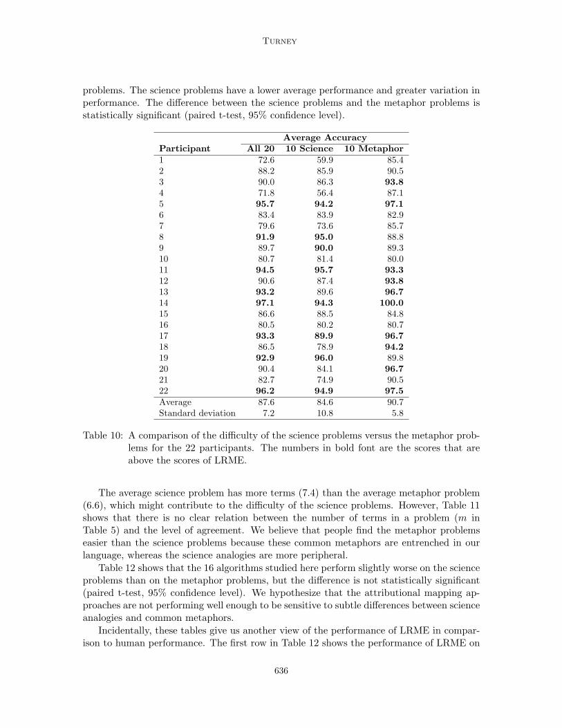
problems. The science problems have a lower average performance and greater variation inperformance. The difference between the science problems and the metaphor problems isstatistically significant (paired t-test, 95% confidence level).

Average AccuracyParticipant All 20 10 Science 10 Metaphor1 72.6 59.9 85.42 88.2 85.9 90.53 90.0 86.3 93.84 71.8 56.4 87.15 95.7 94.2 97.16 83.4 83.9 82.97 79.6 73.6 85.78 91.9 95.0 88.89 89.7 90.0 89.310 80.7 81.4 80.011 94.5 95.7 93.312 90.6 87.4 93.813 93.2 89.6 96.714 97.1 94.3 100.015 86.6 88.5 84.816 80.5 80.2 80.717 93.3 89.9 96.718 86.5 78.9 94.219 92.9 96.0 89.820 90.4 84.1 96.721 82.7 74.9 90.522 96.2 94.9 97.5Average 87.6 84.6 90.7Standard deviation 7.2 10.8 5.8

Table 10: A comparison of the difficulty of the science problems versus the metaphor prob-lems for the 22 participants. The numbers in bold font are the scores that areabove the scores of LRME.

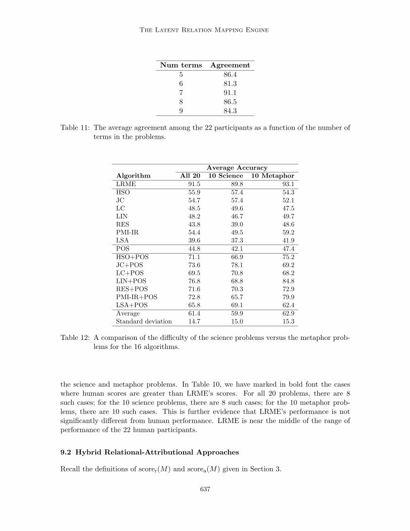
The average science problem has more terms (7.4) than the average metaphor problem(6.6), which might contribute to the difficulty of the science problems. However, Table 11shows that there is no clear relation between the number of terms in a problem (m inTable 5) and the level of agreement. We believe that people find the metaphor problemseasier than the science problems because these common metaphors are entrenched in ourlanguage, whereas the science analogies are more peripheral.

Table 12 shows that the 16 algorithms studied here perform slightly worse on the scienceproblems than on the metaphor problems, but the difference is not statistically significant(paired t-test, 95% confidence level). We hypothesize that the attributional mapping ap-proaches are not performing well enough to be sensitive to subtle differences between scienceanalogies and common metaphors.

Incidentally, these tables give us another view of the performance of LRME in compar-ison to human performance. The first row in Table 12 shows the performance of LRME on

636


Num terms Agreement5 86.46 81.37 91.18 86.59 84.3

Table 11: The average agreement among the 22 participants as a function of the number ofterms in the problems.

Average AccuracyAlgorithm All 20 10 Science 10 MetaphorLRME 91.5 89.8 93.1HSO 55.9 57.4 54.3JC 54.7 57.4 52.1LC 48.5 49.6 47.5LIN 48.2 46.7 49.7RES 43.8 39.0 48.6PMI-IR 54.4 49.5 59.2LSA 39.6 37.3 41.9POS 44.8 42.1 47.4HSO+POS 71.1 66.9 75.2JC+POS 73.6 78.1 69.2LC+POS 69.5 70.8 68.2LIN+POS 76.8 68.8 84.8RES+POS 71.6 70.3 72.9PMI-IR+POS 72.8 65.7 79.9LSA+POS 65.8 69.1 62.4Average 61.4 59.9 62.9Standard deviation 14.7 15.0 15.3

Table 12: A comparison of the difficulty of the science problems versus the metaphor prob-lems for the 16 algorithms.

the science and metaphor problems. In Table 10, we have marked in bold font the caseswhere human scores are greater than LRME’s scores. For all 20 problems, there are 8such cases; for the 10 science problems, there are 8 such cases; for the 10 metaphor prob-lems, there are 10 such cases. This is further evidence that LRME’s performance is notsignificantly different from human performance. LRME is near the middle of the range ofperformance of the 22 human participants.

9.2 Hybrid Relational-Attributional Approaches

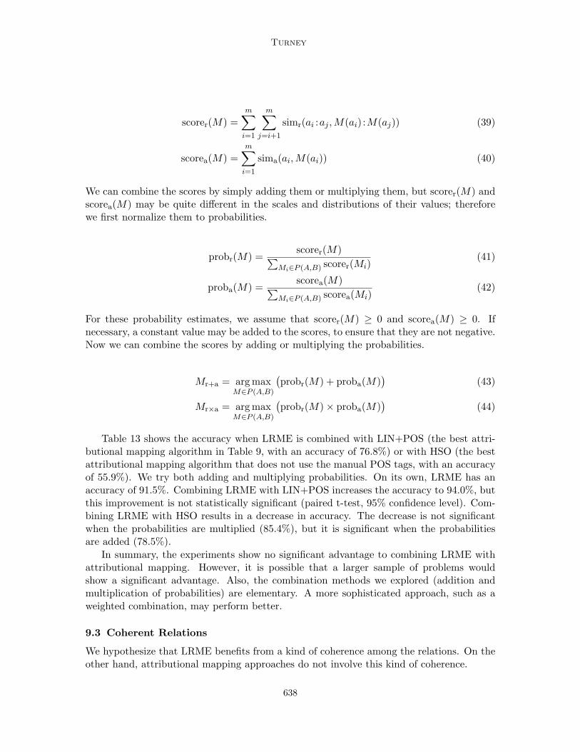
Recall the definitions of scorer(M) and scorea(M) given in Section 3.

637

Turney

scorer(M) =m∑

i=1

m∑j=i+1


scorea(M) =m∑

i=1


We can combine the scores by simply adding them or multiplying them, but scorer(M) andscorea(M) may be quite different in the scales and distributions of their values; thereforewe first normalize them to probabilities.

probr(M) =scorer(M)∑

Mi∈P (A,B) scorer(Mi)(41)

proba(M) =scorea(M)∑

Mi∈P (A,B) scorea(Mi)(42)

For these probability estimates, we assume that scorer(M) ≥ 0 and scorea(M) ≥ 0. Ifnecessary, a constant value may be added to the scores, to ensure that they are not negative.Now we can combine the scores by adding or multiplying the probabilities.

Mr+a = arg maxM∈P (A,B)

(probr(M) + proba(M)

)(43)

Mr×a = arg maxM∈P (A,B)

(probr(M)× proba(M)

)(44)

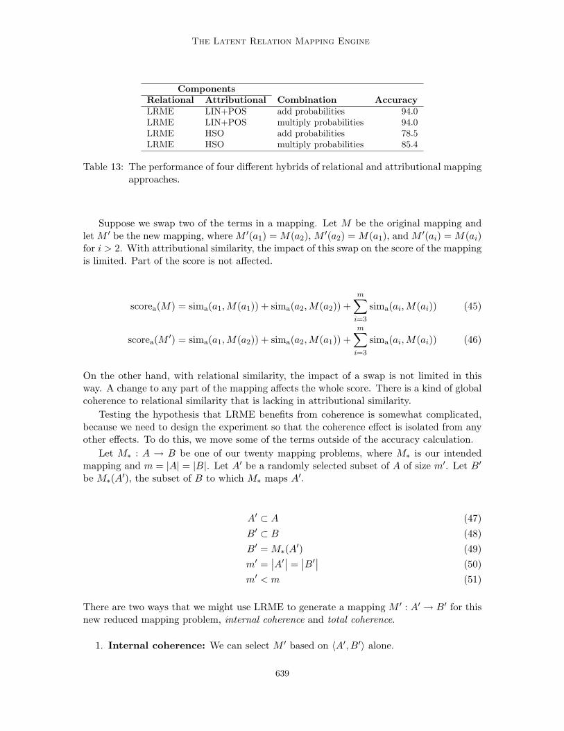
Table 13 shows the accuracy when LRME is combined with LIN+POS (the best attri-butional mapping algorithm in Table 9, with an accuracy of 76.8%) or with HSO (the bestattributional mapping algorithm that does not use the manual POS tags, with an accuracyof 55.9%). We try both adding and multiplying probabilities. On its own, LRME has anaccuracy of 91.5%. Combining LRME with LIN+POS increases the accuracy to 94.0%, butthis improvement is not statistically significant (paired t-test, 95% confidence level). Com-bining LRME with HSO results in a decrease in accuracy. The decrease is not significantwhen the probabilities are multiplied (85.4%), but it is significant when the probabilitiesare added (78.5%).

In summary, the experiments show no significant advantage to combining LRME withattributional mapping. However, it is possible that a larger sample of problems wouldshow a significant advantage. Also, the combination methods we explored (addition andmultiplication of probabilities) are elementary. A more sophisticated approach, such as aweighted combination, may perform better.

9.3 Coherent Relations

We hypothesize that LRME benefits from a kind of coherence among the relations. On theother hand, attributional mapping approaches do not involve this kind of coherence.

638


ComponentsRelational Attributional Combination AccuracyLRME LIN+POS add probabilities 94.0LRME LIN+POS multiply probabilities 94.0LRME HSO add probabilities 78.5LRME HSO multiply probabilities 85.4

Table 13: The performance of four different hybrids of relational and attributional mappingapproaches.

Suppose we swap two of the terms in a mapping. Let M be the original mapping andlet M ′ be the new mapping, where M ′(a1) = M(a2), M ′(a2) = M(a1), and M ′(ai) = M(ai)for i > 2. With attributional similarity, the impact of this swap on the score of the mappingis limited. Part of the score is not affected.

scorea(M) = sima(a1, M(a1)) + sima(a2, M(a2)) +m∑

i=3


scorea(M ′) = sima(a1, M(a2)) + sima(a2, M(a1)) +m∑

i=3


On the other hand, with relational similarity, the impact of a swap is not limited in thisway. A change to any part of the mapping affects the whole score. There is a kind of globalcoherence to relational similarity that is lacking in attributional similarity.

Testing the hypothesis that LRME benefits from coherence is somewhat complicated,because we need to design the experiment so that the coherence effect is isolated from anyother effects. To do this, we move some of the terms outside of the accuracy calculation.

Let M∗ : A → B be one of our twenty mapping problems, where M∗ is our intendedmapping and m = |A| = |B|. Let A′ be a randomly selected subset of A of size m′. Let B′

be M∗(A′), the subset of B to which M∗ maps A′.

A′ ⊂ A (47)B′ ⊂ B (48)B′ = M∗(A′) (49)m′ =

∣∣A′∣∣ =∣∣B′∣∣ (50)

m′ < m (51)

There are two ways that we might use LRME to generate a mapping M ′ : A′ → B′ for thisnew reduced mapping problem, internal coherence and total coherence.

1. Internal coherence: We can select M ′ based on 〈A′, B′〉 alone.

639

Turney

A′ = {a1, ..., am′} (52)B′ = {b1, ..., bm′} (53)

M ′ = arg maxM∈P (A′,B′)

m′∑i=1

m′∑j=i+1


In this case, M ′ is chosen based only on the relations that are internal to 〈A′, B′〉.2. Total coherence: We can select M ′ based on 〈A, B〉 and the knowledge that M ′

must satisfy the constraint that M ′(A′) = B′. (This knowledge is also embedded ininternal coherence.)

A = {a1, ..., am} (55)B = {b1, ..., bm} (56)

P ′(A, B) ={M | M ∈ P (A, B) and M(A′) = B′} (57)

M ′ = arg maxM∈P ′(A,B)

m∑i=1

m∑j=i+1


In this case, M ′ is chosen using both the relations that are internal to 〈A′, B′〉 andother relations in 〈A, B〉 that are external to 〈A′, B′〉.

Suppose that we calculate the accuracy of these two methods based only on the sub-problem 〈A′, B′〉. At first it might seem that there is no advantage to total coherence,because it must explore a larger space of possible mappings than internal coherence (since|P ′(A, B)| is larger than |P (A′, B′)|), but the additional terms that it explores are notinvolved in calculating the accuracy. However, we hypothesize that total coherence willhave a higher accuracy than internal coherence, because the additional external relationshelp to select the correct mapping.

To test this hypothesis, we set m′ to 3 and we randomly generated ten new reducedmapping problems for each of the twenty problems (i.e., a total of 200 new problems of size3). The average accuracy of internal coherence was 93.3%, whereas the average accuracyof total coherence was 97.3%. The difference is statistically significant (paired t-test, 95%confidence level).

On the other hand, the attributional mapping approaches cannot benefit from totalcoherence, because there is no connection between the attributes that are in 〈A′, B′〉 andthe attributes that are outside. We can decompose scorea(M) into two independent parts.

640


A′′ = A \A′ (59)A = A′ ∪A′′ (60)

P ′(A, B) ={M | M ∈ P (A, B) and M(A′) = B′} (61)

M ′ = arg maxM∈P ′(A,B)

∑ai∈A


= arg maxM∈P ′(A,B)

∑ai∈A′

sima(ai, M(ai)) +∑

ai∈A′′

sima(ai, M(ai))

(63)

These two parts can be optimized independently. Thus the terms that are external to〈A′, B′〉 have no influence on the part of M ′ that covers 〈A′, B′〉.

Relational mapping cannot be decomposed into independent parts in this way, becausethe relations connect the parts. This gives relational mapping approaches an inherentadvantage over attributional mapping approaches.

To confirm this analysis, we compared internal and total coherence using LIN+POSon the same 200 new problems of size 3. The average accuracy of internal coherence was88.0%, whereas the average accuracy of total coherence was 87.0%. The difference is notstatistically significant (paired t-test, 95% confidence level). (The only reason that there isany difference is that, when two mappings have the same score, we break the ties randomly.This causes random variation in the accuracy.)

The benefit from coherence suggests that we can make analogy mapping problems easierfor LRME by adding more terms. The difficulty is that the new terms cannot be randomlychosen; they must fit with the logic of the analogy and not overlap with the existing terms.

Of course, this is not the only important difference between the relational and attribu-tional mapping approaches. We believe that the most important difference is that relationsare more reliable and more general than attributes, when using past experiences to makepredictions about the future (Hofstadter, 2001; Gentner, 2003). Unfortunately, this hypoth-esis is more difficult to evaluate experimentally than our hypothesis about coherence.

10. Related Work

French (2002) gives a good survey of computational approaches to analogy-making, from theperspective of cognitive science (where the emphasis is on how well computational systemsmodel human performance, rather than how well the systems perform). We will sample afew systems from his survey and add a few more that were not mentioned.

French (2002) categorizes analogy-making systems as symbolic, connectionist, or symbolic-connectionist hybrids. Gardenfors (2004) proposes another category of representationalsystems for AI and cognitive science, which he calls conceptual spaces. These spatial or geo-metric systems are common in information retrieval and machine learning (Widdows, 2004;van Rijsbergen, 2004). An influential example is Latent Semantic Analysis (Landauer &Dumais, 1997). The first spatial approaches to analogy-making began to appear around thesame time as French’s (2002) survey. LRME takes a spatial approach to analogy-making.

641

Turney

10.1 Symbolic Approaches

Computational approaches to analogy-making date back to Analogy (Evans, 1964) andArgus (Reitman, 1965). Both of these systems were designed to solve proportional analogies(analogies in which |A| = |B| = 2; see Section 4). Analogy could solve proportionalanalogies with simple geometric figures and Argus could solve simple word analogies. Thesesystems used hand-coded rules and were only able to solve the limited range of problemsthat their designers had anticipated and coded in the rules.

French (2002) cites Structure Mapping Theory (SMT) (Gentner, 1983) and the StructureMapping Engine (SME) (Falkenhainer et al., 1989) as the prime examples of symbolicapproaches:

SMT is unquestionably the most influential work to date on the modeling ofanalogy-making and has been applied in a wide range of contexts ranging fromchild development to folk physics. SMT explicitly shifts the emphasis in analogy-making to the structural similarity between the source and target domains. Twomajor principles underlie SMT:

• the relation-matching principle: good analogies are determined by map-pings of relations and not attributes (originally only identical predicateswere mapped) and

• the systematicity principle: mappings of coherent systems of relations arepreferred over mappings of individual relations.

This structural approach was intended to produce a domain-independent map-ping process.

LRME follows both of these principles. LRME uses only relational similarity; no attribu-tional similarity is involved (see Section 7.1). Coherent systems of relations are preferredover mappings of individual relations (see Section 9.3). However, the spatial (statistical,corpus-based) approach of LRME is quite different from the symbolic (logical, hand-coded)approach of SME.

Martin (1992) uses a symbolic approach to handle conventional metaphors. Gentner,Bowdle, Wolff, and Boronat (2001) argue that novel metaphors are processed as analogies,but conventional metaphors are recalled from memory without special processing. However,the line between conventional and novel metaphor can be unclear.

Dolan (1995) describes an algorithm that can extract conventional metaphors from adictionary. A semantic parser is used to extract semantic relations from the LongmanDictionary of Contemporary English (LDOCE). A symbolic algorithm finds metaphoricalrelations between words, using the extracted relations.

Veale (2003, 2004) has developed a symbolic approach to analogy-making, using Word-Net as a lexical resource. Using a spreading activation algorithm, he achieved a score of43.0% on a set of 374 multiple-choice lexical proportional analogy questions from the SATcollege entrance test (Veale, 2004).

Lepage (1998) has demonstrated that a symbolic approach to proportional analogies canbe used for morphology processing. Lepage and Denoual (2005) apply a similar approachto machine translation.

642


10.2 Connectionist Approaches

Connectionist approaches to analogy-making include ACME (Holyoak & Thagard, 1989)and LISA (Hummel & Holyoak, 1997). Like symbolic approaches, these systems use hand-coded knowledge representations, but the search for mappings takes a connectionist ap-proach, in which there are nodes with weights that are incrementally updated over time,until the system reaches a stable state.

10.3 Symbolic-Connectionist Hybrid Approaches

The third family examined by French (2002) is hybrid approaches, containing elementsof both the symbolic and connectionist approaches. Examples include Copycat (Mitchell,1993) and Tabletop (French, 1995). Much of the work in the Fluid Analogies ResearchGroup (FARG) concerns symbolic-connectionist hybrids (Hofstadter & FARG, 1995).

10.4 Spatial Approaches

Marx, Dagan, Buhmann, and Shamir (2002) present the coupled clustering algorithm, whichuses a feature vector representation to find analogies in collections of text. For example,given documents on Buddhism and Christianity, it finds related terms, such as {school,Mahayana, Zen} for Buddhism and {tradition, Catholic, Protestant} for Christianity.

Mason (2004) describes the CorMet system for extracting conventional metaphors fromtext. CorMet is based on clustering feature vectors that represent the selectional preferencesof verbs. Given keywords for the source domain laboratory and the target domain finance,it is able to discover mappings such as liquid → income and container → institution.

Turney, Littman, Bigham, and Shnayder (2003) present a system for solving lexicalproportional analogy questions from the SAT college entrance test, which combines thirteendifferent modules. Twelve of the modules use either attributional similarity or a symbolicapproach to relational similarity, but one module uses a spatial (feature vector) approachto measuring relational similarity. This module worked much better than any of the othermodules; therefore, it was studied in more detail by Turney and Littman (2005). Therelation between a pair of words is represented by a vector, in which the elements are patternfrequencies. This is similar to LRME, but one important difference is that Turney andLittman (2005) used a fixed, hand-coded set of 128 patterns, whereas LRME automaticallygenerates a variable number of patterns from the given corpus (33,240 patterns in ourexperiments here).

Turney (2005) introduced Latent Relational Analysis (LRA), which was examined morethoroughly by Turney (2006). LRA achieves human-level performance on a set of 374multiple-choice proportional analogy questions from the SAT college entrance exam. LRMEuses a simplified form of LRA. A similar simplification of LRA is used by Turney (2008), ina system for processing analogies, synonyms, antonyms, and associations. The contributionof LRME is to go beyond proportional analogies, to larger systems of analogical mappings.

10.5 General Theories of Analogy and Metaphor

Many theories of analogy-making and metaphor either do not involve computation or theysuggest general principles and concepts that are not specific to any particular computational

643

Turney

approach. The design of LRME has been influenced by several theories of this type (Gentner,1983; Hofstadter & FARG, 1995; Holyoak & Thagard, 1995; Hofstadter, 2001; Gentner,2003).

Lakoff and Johnson (1980) provide extensive evidence that metaphor is ubiquitous inlanguage and thought. We believe that a system for analogy-making should be able tohandle metaphorical language, which is why ten of our analogy problems are derived fromLakoff and Johnson (1980). We agree with their claim that a metaphor does not merelyinvolve a superficial relation between a couple of words; rather, it involves a systematic setof mappings between two domains. Thus our analogy problems involve larger sets of words,beyond proportional analogies.

Holyoak and Thagard (1995) argue that analogy-making is central in our daily thought,and especially in finding creative solutions to new problems. Our ten scientific analogieswere derived from their examples of analogy-making in scientific creativity.

11. Limitations and Future Work

In Section 4, we mentioned ten applications for LRA, and in Section 5 we claimed that theresults of the experiments in Section 9.3 suggest that LRME may perform better than LRAon all ten of these applications, due to its ability to handle bijective analogies when m > 2.Our focus in future work will be testing this hypothesis. In particular, the task of semanticrole labeling, discussed in Section 1, seems to be a good candidate application for LRME.

The input to LRME is simpler than the input to SME (compare Figures 1 and 2 inSection 1 with Table 1), but there is still some human effort involved in creating the input.LRME is not immune to the criticism of Chalmers, French, and Hofstadter (1992), thatthe human who generates the input is doing more work than the computer that makes themappings, although it is not a trivial matter to find the right mapping out of 5,040 (7!)choices.

In future work, we would like to relax the requirement that 〈A, B〉 must be a bijection(see Section 3), by adding irrelevant words (distractors) and synonyms. The mappingalgorithm will be forced to decide what terms to include in the mapping and what termsto leave out.

We would also like to develop an algorithm that can take a proportional analogy (m = 2)as input (e.g., sun:planet::nucleus:electron) and automatically expand it to a larger analogy(m > 2, e.g., Table 2). That is, it would automatically search the corpus for new terms toadd to the analogy.

The next step would be to give the computer only the topic of the source domain (e.g.,solar system) and the topic of the target domain (e.g., atomic structure), and let it workout the rest on its own. This might be possible by combining ideas from LRME with ideasfrom coupled clustering (Marx et al., 2002) and CorMet (Mason, 2004).

It seems that analogy-making is triggered in people when we encounter a problem(Holyoak & Thagard, 1995). The problem defines the target for us, and we immediatelystart searching for a source. Analogical mapping enables us to transfer our knowledge ofthe source to the target, hopefully leading to a solution to the problem. This suggests thatthe input to the ideal analogical mapping algorithm would be simply a statement that there

644


is a problem (e.g., What is the structure of the atom?). Ultimately, the computer mightfind the problems on its own as well. The only input would be a large corpus.

The algorithms we have considered here all perform exhaustive search of the set ofpossible mappings P (A, B). This is acceptable when the sets are small, as they are here,but it will be problematic for larger problems. In future work, it will be necessary to useheuristic search algorithms instead of exhaustive search.

It takes almost 18 hours for LRME to process the twenty mapping problems (Section 7).With better hardware and some changes to the software, this time could be significantlyreduced. For even greater speed, the algorithm could run continuously, building a largedatabase of vector representations of term pairs, so that it is ready to create mappings assoon as a user requests them. This is similar to the vision of Banko and Etzioni (2007).

LRME, like LRA and LSA (Landauer & Dumais, 1997), uses a truncated singular valuedecomposition (SVD) to smooth the matrix. Many other algorithms have been proposedfor smoothing matrices. In our past work with LRA (Turney, 2006), we experimented withNonnegative Matrix Factorization (NMF) (Lee & Seung, 1999), Probabilistic Latent Se-mantic Analysis (PLSA) (Hofmann, 1999), Iterative Scaling (IS) (Ando, 2000), and KernelPrincipal Components Analysis (KPCA) (Scholkopf, Smola, & Muller, 1997). We had someinteresting results with small matrices (around 1000 × 2000), but none of the algorithmsseemed substantially better than truncated SVD, and none of them scaled up to the matrixsizes that we have here (1,662 × 33,240). However, we believe that SVD is not unique, andfuture work is likely to discover a smoothing algorithm that is more efficient and effectivethan SVD. The results in Section 7.2 do not show a significant benefit from SVD. Table 8hints that PPMIC (Bullinaria & Levy, 2007) is more important than SVD.

LRME extracts knowledge from many fragments of text. In Section 7.1, we notedthat we found an average of 1,180 phrases per pair. The information from these 1,180phrases is combined in a vector, to represent the semantic relation for a pair. This isquite different from relation extraction in (for example) the Automatic Content Extraction(ACE) Evaluation.11 The task in ACE is to identify and label a semantic relation in a singlesentence. Semantic role labeling also involves labeling a single sentence (Gildea & Jurafsky,2002).

The contrast between LRME and ACE is analogous to the distinction in cognitivepsychology between semantic and episodic memory. Episodic memory is memory of aspecific event in one’s personal past, whereas semantic memory is memory of basic facts andconcepts, unrelated to any specific event in the past. LRME extracts relational informationthat is independent of any specific sentence, like semantic memory. ACE is concerned withextracting the relation in a specific sentence, like episodic memory. In cognition, episodicmemory and semantic memory work together synergistically. When we experience an event,we use our semantic memory to interpret the event and form a new episodic memory,but semantic memory is itself constructed from our past experiences, our accumulatedepisodic memories. This suggests that there should be a synergy from combining LRME-likesemantic information extraction algorithms with ACE-like episodic information extractionalgorithms.

11. ACE is an annual event that began in 1999. Relation Detection and Characterization (RDC) wasintroduced to ACE in 2001. For more information, see http://www.nist.gov/speech/tests/ace/.

645

Turney

12. Conclusion

Analogy is the core of cognition. We understand the present by analogy to the past. Wepredict the future by analogy to the past and the present. We solve problems by searchingfor analogous situations (Holyoak & Thagard, 1995). Our daily language is saturated withmetaphor (Lakoff & Johnson, 1980), and metaphor is based on analogy (Gentner et al.,2001). To understand human language, to solve human problems, to work with humans,computers must be able to make analogical mappings.

Our best theory of analogy-making is Structure Mapping Theory (Gentner, 1983), butthe Structure Mapping Engine (Falkenhainer et al., 1989) puts too much of the burdenof analogy-making on its human users (Chalmers et al., 1992). LRME is an attempt toshift some of that burden onto the computer, while remaining consistent with the generalprinciples of SMT.

We have shown that LRME is able to solve bijective analogical mapping problems withhuman-level performance. Attributional mapping algorithms (at least, those we have triedso far) are not able to reach this level. This supports SMT, which claims that relations aremore important than attributes when making analogical mappings.

There is still much research to be done. LRME takes some of the load off the humanuser, but formulating the input to LRME is not easy. This paper is an incremental steptowards a future in which computers can make surprising and useful analogies with minimalhuman assistance.

Acknowledgments

Thanks to my colleagues at the Institute for Information Technology for participating inthe experiment in Section 6. Thanks to Charles Clarke and Egidio Terra for their corpus.Thanks to Stefan Buttcher for making Wumpus available and giving me advice on its use.Thanks to Doug Rohde for making SVDLIBC available. Thanks to the WordNet team atPrinceton University for WordNet, Ted Pedersen for the WordNet::Similarity Perl package,and Jason Rennie for the WordNet::QueryData Perl package. Thanks to the LSA teamat the University of Colorado at Boulder for the use of their online demonstration of LSA.Thanks to Deniz Yuret, Andre Vellino, Dedre Gentner, Vivi Nastase, Yves Lepage, DiarmuidO Seaghdha, Roxana Girju, Chris Drummond, Howard Johnson, Stan Szpakowicz, and theanonymous reviewers of JAIR for their helpful comments and suggestions.

Appendix A. Details of the Mapping Problems

In this appendix, we provide detailed information about the twenty mapping problems.Figure 3 shows the instructions that were given to the participants in the experiment inSection 6. These instructions were displayed in their web browsers. Tables 14, 15, 16,and 17 show the twenty mapping problems. The first column gives the problem number(e.g., A1) and a mnemonic that summarizes the mapping (e.g., solar system → atom). Thesecond column gives the source terms and the third column gives the target terms.

The mappings shown in these tables are our intended mappings. The fourth columnshows the percentage of participants who agreed with our intended mappings. For example,

646


Systematic Analogies and Metaphors

Instructions

You will be presented with twenty analogical mapping problems, ten based on scientificanalogies and ten based on common metaphors. A typical problem will look like this:

horse → ? ∇legs → ? ∇hay → ? ∇brain → ? ∇dung → ? ∇

You may click on the drop-down menus above, to see what options are available.

Your task is to construct an analogical mapping; that is, a one-to-one mapping between theitems on the left and the items on the right. For example:

horse → car ∇legs → wheels ∇hay → gasoline ∇brain → driver ∇dung → exhaust ∇

This mapping expresses an analogy between a horse and a car. The horse’s legs are like thecar’s wheels. The horse eats hay and the car consumes gasoline. The horse’s brain controlsthe movement of the horse like the car’s driver controls the movement of the car. The horsegenerates dung as a waste product like the car generates exhaust as a waste product.

You should have no duplicate items in your answers on the right-hand side. If there areany duplicates or missing items (question marks), you will get an error message when yousubmit your answer.

You are welcome to use a dictionary as you work on the problems, if you would find ithelpful.

If you find the above instructions unclear, then please do not continue with this exercise.Your answers to the twenty problems will be used as a standard for evaluating the outputof a computer algorithm; therefore, you should only proceed if you are confident that youunderstand this task.

Figure 3: The instructions for the participants in the experiment in Section 6.

647

Turney

Mapping Source → Target Agreement POSsolar system → atom 86.4 NN

A1 sun → nucleus 100.0 NNplanet → electron 95.5 NN

solar system mass → charge 86.4 NN→ atom attracts → attracts 90.9 VBZ

revolves → revolves 95.5 VBZgravity → electromagnetism 81.8 NNAverage agreement: 90.9water → heat 86.4 NN

A2 flows → transfers 95.5 VBZpressure → temperature 86.4 NN

water flow water tower → burner 72.7 NN→ heat transfer bucket → kettle 72.7 NN

filling → heating 95.5 VBGemptying → cooling 95.5 VBGhydrodynamics → thermodynamics 90.9 NNAverage agreement: 86.9waves → sounds 86.4 NNS

A3 shore → wall 77.3 NNreflects → echoes 95.5 VBZ

waves water → air 95.5 NN→ sounds breakwater → insulation 81.8 NN

rough → loud 63.6 JJcalm → quiet 100.0 JJcrashing → vibrating 54.5 VBGAverage agreement: 81.8combustion → respiration 72.7 NN

A4 fire → animal 95.5 NNfuel → food 90.9 NN

combustion burning → breathing 72.7 VBG→ respiration hot → living 59.1 JJ

intense → vigorous 77.3 JJoxygen → oxygen 77.3 NNcarbon dioxide → carbon dioxide 86.4 NNAverage agreement: 79.0sound → light 86.4 NN

A5 low → red 50.0 JJhigh → violet 54.5 JJ

sound echoes → reflects 100.0 VBZ→ light loud → bright 90.9 JJ

quiet → dim 77.3 JJhorn → lens 95.5 NNAverage agreement: 79.2

Table 14: Science analogy problems A1 to A5, derived from Chapter 8 of Holyoak andThagard (1995).

648


Mapping Source → Target Agreement POSprojectile → planet 100.0 NN

A6 trajectory → orbit 100.0 NNearth → sun 100.0 NN

projectile parabolic → elliptical 100.0 JJ→ planet air → space 100.0 NN

gravity → gravity 90.9 NNattracts → attracts 90.9 VBZAverage agreement: 97.4breeds → species 100.0 NNS

A7 selection → competition 59.1 NNconformance → adaptation 59.1 NN

artificial selection artificial → natural 77.3 JJ→ natural selection popularity → fitness 54.5 NN

breeding → mating 95.5 VBGdomesticated → wild 77.3 JJAverage agreement: 74.7balls → molecules 90.9 NNS

A8 billiards → gas 72.7 NNspeed → temperature 81.8 NN

billiard balls table → container 95.5 NN→ gas molecules bouncing → pressing 77.3 VBG

moving → moving 86.4 VBGslow → cold 100.0 JJfast → hot 100.0 JJAverage agreement: 88.1computer → mind 90.9 NN

A9 processing → thinking 95.5 VBGerasing → forgetting 100.0 VBG

computer write → memorize 72.7 VB→ mind read → remember 54.5 VB

memory → memory 81.8 NNoutputs → muscles 72.7 NNSinputs → senses 90.9 NNSbug → mistake 100.0 NNAverage agreement: 84.3slot machines → bacteria 68.2 NNS

A10 reels → genes 72.7 NNSspinning → mutating 86.4 VBG

slot machine winning → reproducing 90.9 VBG→ bacterial mutation losing → dying 100.0 VBG

Average agreement: 83.6

Table 15: Science analogy problems A6 to A10, derived from Chapter 8 of Holyoak andThagard (1995).

649

Turney

Mapping Source → Target Agreement POSwar → argument 90.9 NN

M1 soldier → debater 100.0 NNdestroy → refute 90.9 VB

war fighting → arguing 95.5 VBG→ argument defeat → acceptance 90.9 NN

attacks → criticizes 95.5 VBZweapon → logic 90.9 NNAverage agreement: 93.5buyer → believer 100.0 NN

M2 merchandise → belief 90.9 NNbuying → accepting 95.5 VBG

buying an item selling → advocating 100.0 VBG→ accepting a belief returning → rejecting 95.5 VBG

valuable → true 95.5 JJworthless → false 95.5 JJAverage agreement: 96.1foundations → reasons 72.7 NNS

M3 buildings → theories 77.3 NNSsupporting → confirming 95.5 VBG

grounds for a building solid → rational 90.9 JJ→ reasons for a theory weak → dubious 95.5 JJ

crack → flaw 95.5 NNAverage agreement: 87.9obstructions → difficulties 100.0 NNS

M4 destination → goal 100.0 NNroute → plan 100.0 NN

impediments to travel traveller → person 100.0 NN→ difficulties travelling → problem solving 100.0 VBG

companion → partner 100.0 NNarriving → succeeding 100.0 VBGAverage agreement: 100.0money → time 95.5 NN

M5 allocate → invest 86.4 VBbudget → schedule 86.4 NN

money effective → efficient 86.4 JJ→ time cheap → quick 50.0 JJ

expensive → slow 59.1 JJAverage agreement: 77.3

Table 16: Common metaphor problems M1 to M5, derived from Lakoff and Johnson (1980).

650


Mapping Source → Target Agreement POSseeds → ideas 90.9 NNS

M6 planted → inspired 95.5 VBDfruitful → productive 81.8 JJ

seeds fruit → product 95.5 NN→ ideas grow → develop 81.8 VB

wither → fail 100.0 VBblossom → succeed 77.3 VBAverage agreement: 89.0machine → mind 95.5 NN

M7 working → thinking 100.0 VBGturned on → awake 100.0 JJ

machine turned off → asleep 100.0 JJ→ mind broken → confused 100.0 JJ

power → intelligence 95.5 NNrepair → therapy 100.0 NNAverage agreement: 98.7object → idea 90.9 NN

M8 hold → understand 81.8 VBweigh → analyze 81.8 VB

object heavy → important 95.5 JJ→ idea light → trivial 95.5 JJ

Average agreement: 89.1follow → understand 100.0 VB

M9 leader → speaker 100.0 NNpath → argument 100.0 NN

following follower → listener 100.0 NN→ understanding lost → misunderstood 86.4 JJ

wanders → digresses 90.9 VBZtwisted → complicated 95.5 JJstraight → simple 100.0 JJAverage agreement: 96.6seeing → understanding 68.2 VBG

M10 light → knowledge 77.3 NNilluminating → explaining 86.4 VBG

seeing darkness → confusion 86.4 NN→ understanding view → interpretation 68.2 NN

hidden → secret 86.4 JJAverage agreement: 78.8

Table 17: Common metaphor problems M6 to M10, derived from Lakoff and Johnson(1980).

651

Turney

in problem A1, 81.8% of the participants (18 out of 22) mapped gravity to electromagnetism.The final column gives the part-of-speech (POS) tags for the source and target terms. Weused the Penn Treebank tags (Santorini, 1990). We assigned these tags manually. Ourintended mappings and our tags were chosen so that mapped terms have the same tags.For example, in A1, sun maps to nucleus, and both sun and nucleus are tagged NN. ThePOS tags are used in the experiments in Section 8. The POS tags are not used by LRMEand they were not shown to the participants in the experiment in Section 6.

References

Ando, R. K. (2000). Latent semantic space: Iterative scaling improves precision of inter-document similarity measurement. In Proceedings of the 23rd Annual ACM SIGIRConference on Research and Development in Information Retrieval (SIGIR-2000), pp.216–223.

Banko, M., & Etzioni, O. (2007). Strategies for lifelong knowledge extraction from the web.In Proceedings of the 4th International Conference on Knowledge Capture (K-CAP2007), pp. 95–102.

Bullinaria, J., & Levy, J. (2007). Extracting semantic representations from word co-occurrence statistics: A computational study. Behavior Research Methods, 39 (3),510–526.

Buttcher, S., & Clarke, C. (2005). Efficiency vs. effectiveness in terabyte-scale informa-tion retrieval. In Proceedings of the 14th Text REtrieval Conference (TREC 2005),Gaithersburg, MD.

Chalmers, D. J., French, R. M., & Hofstadter, D. R. (1992). High-level perception, repre-sentation, and analogy: A critique of artificial intelligence methodology. Journal ofExperimental & Theoretical Artificial Intelligence, 4 (3), 185–211.

Deerwester, S. C., Dumais, S. T., Landauer, T. K., Furnas, G. W., & Harshman, R. A.(1990). Indexing by latent semantic analysis. Journal of the American Society forInformation Science (JASIS), 41 (6), 391–407.

Dolan, W. B. (1995). Metaphor as an emergent property of machine-readable dictionar-ies. In Proceedings of the AAAI 1995 Spring Symposium Series: Representation andAcquisition of Lexical Knowledge: Polysemy, Ambiguity and Generativity, pp. 27–32.

Evans, T. (1964). A heuristic program to solve geometric-analogy problems. In Proceedingsof the Spring Joint Computer Conference, pp. 327–338.

Falkenhainer, B., Forbus, K. D., & Gentner, D. (1989). The structure-mapping engine:Algorithm and examples. Artificial Intelligence, 41 (1), 1–63.

Firth, J. R. (1957). A synopsis of linguistic theory 1930–1955. In Studies in LinguisticAnalysis, pp. 1–32. Blackwell, Oxford.

Forbus, K., Usher, J., Lovett, A., Lockwood, K., & Wetzel, J. (2008). Cogsketch: Open-domain sketch understanding for cognitive science research and for education. InProceedings of the Fifth Eurographics Workshop on Sketch-Based Interfaces and Mod-eling, Annecy, France.

652


Forbus, K. D., Riesbeck, C., Birnbaum, L., Livingston, K., Sharma, A., & Ureel, L. (2007). Aprototype system that learns by reading simplified texts. In AAAI Spring Symposiumon Machine Reading, Stanford University, California.

French, R. (1995). The Subtlety of Sameness: A Theory and Computer Model of Analogy-Making. MIT Press, Cambridge, MA.

French, R. M. (2002). The computational modeling of analogy-making. Trends in CognitiveSciences, 6 (5), 200–205.

Gardenfors, P. (2004). Conceptual Spaces: The Geometry of Thought. MIT Press.

Gentner, D. (1983). Structure-mapping: A theoretical framework for analogy. CognitiveScience, 7 (2), 155–170.

Gentner, D. (1991). Language and the career of similarity. In Gelman, S., & Byrnes, J.(Eds.), Perspectives on Thought and Language: Interrelations in Development, pp.225–277. Cambridge University Press.

Gentner, D. (2003). Why we’re so smart. In Gentner, D., & Goldin-Meadow, S. (Eds.),Language in Mind: Advances in the Study of Language and Thought, pp. 195–235.MIT Press.

Gentner, D., Bowdle, B. F., Wolff, P., & Boronat, C. (2001). Metaphor is like analogy. InGentner, D., Holyoak, K. J., & Kokinov, B. N. (Eds.), The analogical mind: Perspec-tives from Cognitive Science, pp. 199–253. MIT Press, Cambridge, MA.

Gildea, D., & Jurafsky, D. (2002). Automatic labeling of semantic roles. ComputationalLinguistics, 28 (3), 245–288.

Girju, R., Nakov, P., Nastase, V., Szpakowicz, S., Turney, P., & Yuret, D. (2007). Semeval-2007 task 04: Classification of semantic relations between nominals. In Proceedingsof the Fourth International Workshop on Semantic Evaluations (SemEval 2007), pp.13–18, Prague, Czech Republic.

Golub, G. H., & Van Loan, C. F. (1996). Matrix Computations (Third edition). JohnsHopkins University Press, Baltimore, MD.

Hawkins, J., & Blakeslee, S. (2004). On Intelligence. Henry Holt.

Hirst, G., & St-Onge, D. (1998). Lexical chains as representations of context for the detectionand correction of malapropisms. In Fellbaum, C. (Ed.), WordNet: An ElectronicLexical Database, pp. 305–332. MIT Press.

Hofmann, T. (1999). Probabilistic Latent Semantic Indexing. In Proceedings of the 22ndAnnual ACM Conference on Research and Development in Information Retrieval (SI-GIR ’99), pp. 50–57, Berkeley, California.

Hofstadter, D. (2001). Epilogue: Analogy as the core of cognition. In Gentner, D., Holyoak,K. J., & Kokinov, B. N. (Eds.), The Analogical Mind: Perspectives from CognitiveScience, pp. 499–538. MIT Press.

Hofstadter, D., & FARG (1995). Fluid Concepts and Creative Analogies: Computer Modelsof the Fundamental Mechanisms of Thought. Basic Books, New York, NY.

653

Turney

Holyoak, K., & Thagard, P. (1989). Analogical mapping by constraint satisfaction. CognitiveScience, 13, 295–355.

Holyoak, K., & Thagard, P. (1995). Mental Leaps. MIT Press.

Hummel, J., & Holyoak, K. (1997). Distributed representations of structure: A theory ofanalogical access and mapping. Psychological Review, 104, 427–466.

Jiang, J. J., & Conrath, D. W. (1997). Semantic similarity based on corpus statisticsand lexical taxonomy. In Proceedings of the International Conference on Research inComputational Linguistics (ROCLING X), pp. 19–33, Tapei, Taiwan.

Kilgarriff, A. (1997). I don’t believe in word senses. Computers and the Humanities, 31,91–113.

Lakoff, G., & Johnson, M. (1980). Metaphors We Live By. University Of Chicago Press.

Landauer, T. K., & Dumais, S. T. (1997). A solution to Plato’s problem: The latent se-mantic analysis theory of the acquisition, induction, and representation of knowledge.Psychological Review, 104 (2), 211–240.

Leacock, C., & Chodrow, M. (1998). Combining local context and WordNet similarity forword sense identification. In Fellbaum, C. (Ed.), WordNet: An Electronic LexicalDatabase. MIT Press.

Lee, D. D., & Seung, H. S. (1999). Learning the parts of objects by nonnegative matrixfactorization. Nature, 401, 788–791.

Lepage, Y. (1998). Solving analogies on words: An algorithm. In Proceedings of the 36thAnnual Conference of the Association for Computational Linguistics, pp. 728–735.

Lepage, Y., & Denoual, E. (2005). Purest ever example-based machine translation: Detailedpresentation and assessment. Machine Translation, 19 (3), 251–282.

Lin, D. (1998). An information-theoretic definition of similarity. In Proceedings of the 15thInternational Conference on Machine Learning (ICML-98).

Martin, J. H. (1992). Computer understanding of conventional metaphoric language. Cog-nitive Science, 16 (2), 233–270.

Marx, Z., Dagan, I., Buhmann, J., & Shamir, E. (2002). Coupled clustering: A methodfor detecting structural correspondence. Journal of Machine Learning Research, 3,747–780.

Mason, Z. (2004). CorMet: A computational, corpus-based conventional metaphor extrac-tion system. Computational Linguistics, 30 (1), 23–44.

Minsky, M. (1986). The Society of Mind. Simon & Schuster, New York, NY.

Mitchell, M. (1993). Analogy-Making as Perception: A Computer Model. MIT Press, Cam-bridge, MA.

Nastase, V., & Szpakowicz, S. (2003). Exploring noun-modifier semantic relations. InFifth International Workshop on Computational Semantics (IWCS-5), pp. 285–301,Tilburg, The Netherlands.

Reitman, W. R. (1965). Cognition and Thought: An Information Processing Approach. JohnWiley and Sons, New York, NY.

654


Resnik, P. (1995). Using information content to evaluate semantic similarity in a taxonomy.In Proceedings of the 14th International Joint Conference on Artificial Intelligence(IJCAI-95), pp. 448–453, San Mateo, CA. Morgan Kaufmann.

Rosario, B., & Hearst, M. (2001). Classifying the semantic relations in noun-compoundsvia a domain-specific lexical hierarchy. In Proceedings of the 2001 Conference onEmpirical Methods in Natural Language Processing (EMNLP-01), pp. 82–90.

Santorini, B. (1990). Part-of-speech tagging guidelines for the Penn Treebank Project. Tech.rep., Department of Computer and Information Science, University of Pennsylvania.(3rd revision, 2nd printing).

Scholkopf, B., Smola, A. J., & Muller, K.-R. (1997). Kernel principal component analysis. InProceedings of the International Conference on Artificial Neural Networks (ICANN-1997), pp. 583–588, Berlin.

Turney, P. D. (2001). Mining the Web for synonyms: PMI-IR versus LSA on TOEFL. InProceedings of the Twelfth European Conference on Machine Learning (ECML-01),pp. 491–502, Freiburg, Germany.

Turney, P. D. (2005). Measuring semantic similarity by latent relational analysis. In Pro-ceedings of the Nineteenth International Joint Conference on Artificial Intelligence(IJCAI-05), pp. 1136–1141, Edinburgh, Scotland.

Turney, P. D. (2006). Similarity of semantic relations. Computational Linguistics, 32 (3),379–416.

Turney, P. D. (2008). A uniform approach to analogies, synonyms, antonyms, and as-sociations. In Proceedings of the 22nd International Conference on ComputationalLinguistics (Coling 2008), pp. 905–912, Manchester, UK.

Turney, P. D., & Littman, M. L. (2005). Corpus-based learning of analogies and semanticrelations. Machine Learning, 60 (1–3), 251–278.

Turney, P. D., Littman, M. L., Bigham, J., & Shnayder, V. (2003). Combining independentmodules to solve multiple-choice synonym and analogy problems. In Proceedings ofthe International Conference on Recent Advances in Natural Language Processing(RANLP-03), pp. 482–489, Borovets, Bulgaria.

van Rijsbergen, C. J. (2004). The Geometry of Information Retrieval. Cambridge UniversityPress, Cambridge, UK.

Veale, T. (2003). The analogical thesaurus. In Proceedings of the 15th Innovative Ap-plications of Artificial Intelligence Conference (IAAI 2003), pp. 137–142, Acapulco,Mexico.

Veale, T. (2004). WordNet sits the SAT: A knowledge-based approach to lexical analogy. InProceedings of the 16th European Conference on Artificial Intelligence (ECAI 2004),pp. 606–612, Valencia, Spain.

Widdows, D. (2004). Geometry and Meaning. Center for the Study of Language andInformation, Stanford, CA.

Yan, J., & Forbus, K. D. (2005). Similarity-based qualitative simulation. In Proceedings ofthe 27th Annual Meeting of the Cognitive Science Society, Stresa, Italy.

655

the latent relation mapping engine: algorithm and experimentscogprints.org/6305/1/nrc-50738.pdf ·...

Documents