Applied Mathematics, 2016, 7, 927-938 Published Online May 2016 in SciRes. http://www.scirp.org/journal/am http://dx.doi.org/10.4236/am.2016.79083

How to cite this paper: Chen, P.Y.P. (2016) The Lanczos-Chebyshev Pseudospectral Method for Solution of Differential Eq-uations. Applied Mathematics, 7, 927-938. http://dx.doi.org/10.4236/am.2016.79083

The Lanczos-Chebyshev Pseudospectral Method for Solution of Differential Equations Peter Y. P. Chen School of Mechanical and Manufacturing Engineering, University of New South Wales, Sydney, Australia

Received 9 December 2015; accepted 24 May 2016; published 27 May 2016

Copyright © 2016 by author and Scientific Research Publishing Inc. This work is licensed under the Creative Commons Attribution International License (CC BY). http://creativecommons.org/licenses/by/4.0/

Abstract In this paper, we propose to replace the Chebyshev series used in pseudospectral methods with the equivalent Chebyshev economized power series that can be evaluated more rapidly. We keep the rest of the implementation the same as the spectral method so that there is no new mathemat-ical principle involved. We show by numerical examples that the new approach works well and there is indeed no significant loss of solution accuracy. The advantages of using power series also include simplicity in its formulation and implementation such that it could be used for complex systems. We investigate the important issue of collocation point selection. Our numerical results indicate that there is a clear accuracy advantage of using collocation points corresponding to roots of the Chebyshev polynomial.

Keywords Solution of Differential Equations, Chebyshev Economized Power Series, Collocation Point Selection, Lanczos-Chebyshev Pseudospectral Method

1. Introduction The basic idea of the spectral methods is to solve differential equations using truncated series expansions [1]. The basis functions chosen for this purpose—for example, Chebyshev polynomials—must be linearly indepen-dent and orthogonal. The methods are implemented in terms of the expansion coefficients [2]. When a differen-tial equation involves variable coefficients, it is more convenient to use the pseudospectral methods, employing collocation at selected points. Among them, the Chebyshev pseudospectral (CPS) methods are the most com-monly used [2] [3]. In general, the collocation approach does not require basis functions to be orthogonal. For

P. Y. P. Chen

928

example, splines [4], canonical polynomials [5], or even mesh-free formulations, based on specially constructed functions [6], had been proposed. So far, none of the non-orthogonal approaches could compete with the stan-dard pseudospectral methods in popularity because there is no clear and decisive advantage in those alternatives.

The idea of using simple power series to generate solution approximation is well known. It is also a well- known fact that pure monomial powers form a terribly ill-conditioned base for all but the very simplest problems. However, this restriction could be overcome. In a number of publications it has been reported that recursive formulations could be used to derive combinations of power functions given under the name canonical polyno-mials [5] [7] [8]. This approach could be considered as too laborious, as the procedures are complex and a set of different canonical polynomials has to be developed for each particular problem. It has also been reported that vast improvement could be achieved if an operational formulation is used [9]. In this alternative approach, there is no implicit use of any recursive relationships. Instead, a series of matrix operations are used, including diffe-rentiation, power multiplication etc. However, the formulation still directly involves linear differential operators of a given problem and the polynomial basis so found is applicable only for that specific problem.

In this paper we describe an efficient alternative based on the replacement of series expansion solutions using orthogonal polynomials such as Chebyshev polynomials with the equivalent Chebyshev economized power se-ries. We are taking full advantage of the collocation approach so that the basis of our approximation is just only the simple power functions that could be used universally for all problems. Just like the operational approach [9], a series of matrix operations are needed. However, the formulation and implementation are expected to be much simpler as the polynomial basis need not to be specifically developed. As Chebyshev economized series are used, best solution accuracy based on the number of terms used can be assured uniformly over the entire domain of interest. We could show numerically that there is no loss of accuracy, if the economized series is based on the collocation points chosen at roots of the Chebyshev polynomial, as originally proposed by Lanczos [10] [11]. We have called this method the Lanczos-Chebyshev Pseudospectral (LCPS) method. We should point out that the use of Chebyshev economized power series has been reported previously [12]. The implementation given is based on a recursive formulation. As a result, this particular reported approach lacks the simplicity that charac-terized the LCPS method.

There are, however, a number of issues that could affect the numerical performance of various methods. To retain the spectral accuracy, pseudospectral formulations employ orthogonal-polynomial series. In implementing those classical pseudospectral methods, the series expansions are often replaced by function values at the collo-cation points in the physical space [2] [13]. Thus, solutions are sought only at the collocation points. If global solutions are required, such as in some nonlinear problems, they can only be obtained from values at grid points by executing some more than trivial numerical routines. For the CPS methods, deriving derivatives from the Chebyshev series results in loss of accuracy [14] [15]. The operation is also expensive in computer execution time, needing O(N^2) operations where N is the number of grid points used. For FFT, the operations are O(NlogN), although in here N is a much larger number than that used in the CPS methods. In contrast, with the series formulation, we are able to restrict the number of operations required to evaluate a function or a derivative to O(2N). In a simulation requiring many evaluations such in an iterative procedure for nonlinear problems or in a long evolution history of a transient problem, a great deal of speed could be gained with no penalty in extra and complicated program development.

Nevertheless, there are good reasons for the pseudospectral methods to remain so popular among the numeri-cal analysts. The methods can be used to solve a wide range of problems, not just in 1D but also 2D and possibly 3D. In almost every case, to achieve the same degree of accuracy, far fewer grid points are required than in the case of other numerical methods. There is the freedom to divide a given domain into a number of sub-domains, gaining many numerical advantages [16] [17]. The formulations involved can be easily programmed to select grids and the number of terms used in the series expansion. The availability of an appropriate commercial pro-gram package [18] [19] is also an attraction. It should be mentioned that all these advantages are retained in the LCPS method with the commercial package as the only exception.

As the formulation based on the power series is simple to implement, it is expected that it would be easy to use LCPS method to solve complex mathematical models resulting from modern sophisticated applications. We have already used the LCPS method to solve wave propagation in a complex system involving special purpose designed metamaterials and photonic crystals [20]. In this present paper we deal only with problems involving one spatial dimension. We have already extended the LCPS method to solve stationary wave-propagation prob-lems in two-dimension [21]. This type of problems could not be readily solved by means of other available nu-merical methods.

P. Y. P. Chen

929

In this paper, we provide details of the formulation of the LCPS method in Section 2, including treatment of domain subdivision. In Section 3, we use several of examples that have either analytical or known numerical solutions, to show the efficiency of the LCPS method. Along with these examples, we test practical issues, such as the selection of collocation points, how one can overcome reduced accuracy in approximating derivatives, and how to achieve the best management of the collocation points. Conclusions are presented in Section 4.

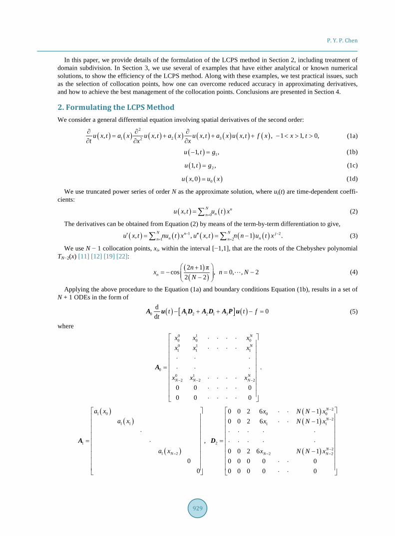
2. Formulating the LCPS Method We consider a general differential equation involving spatial derivatives of the second order:

( ) ( ) ( ) ( ) ( ) ( ) ( ) ( )2

1 2 32, , , , , 1 1, 0,u x t a x u x t a x u x t a x u x t f x x tt xx∂ ∂ ∂

= + + + − < > >∂ ∂∂

(1a)

( ) 11, ,u t g− = (1b)

( ) 2 ,1,u t g= (1c)

( ) ( )0, 0u x u x= (1d)

We use truncated power series of order N as the approximate solution, where ui(t) are time-dependent coeffi-cients:

( ) ( )0, N n

nnu x t u t x

== ∑ (2)

The derivatives can be obtained from Equation (2) by means of the term-by-term differentiation to give,

( ) ( ) ( ) ( ) ( )1 21 2

, , , 1 .N Nn jn nn n

u x t nu t x u x t n n u t x− −= =

′ ′′= = −∑ ∑ (3)

We use N − 1 collocation points, xi, within the interval [−1,1], that are the roots of the Chebyshev polynomial TN−2(x) [11] [12] [19] [22]:

( )( )

2 1 πcos , 0, , 2

2 2nn

x n NN

+= − = − −

(4)

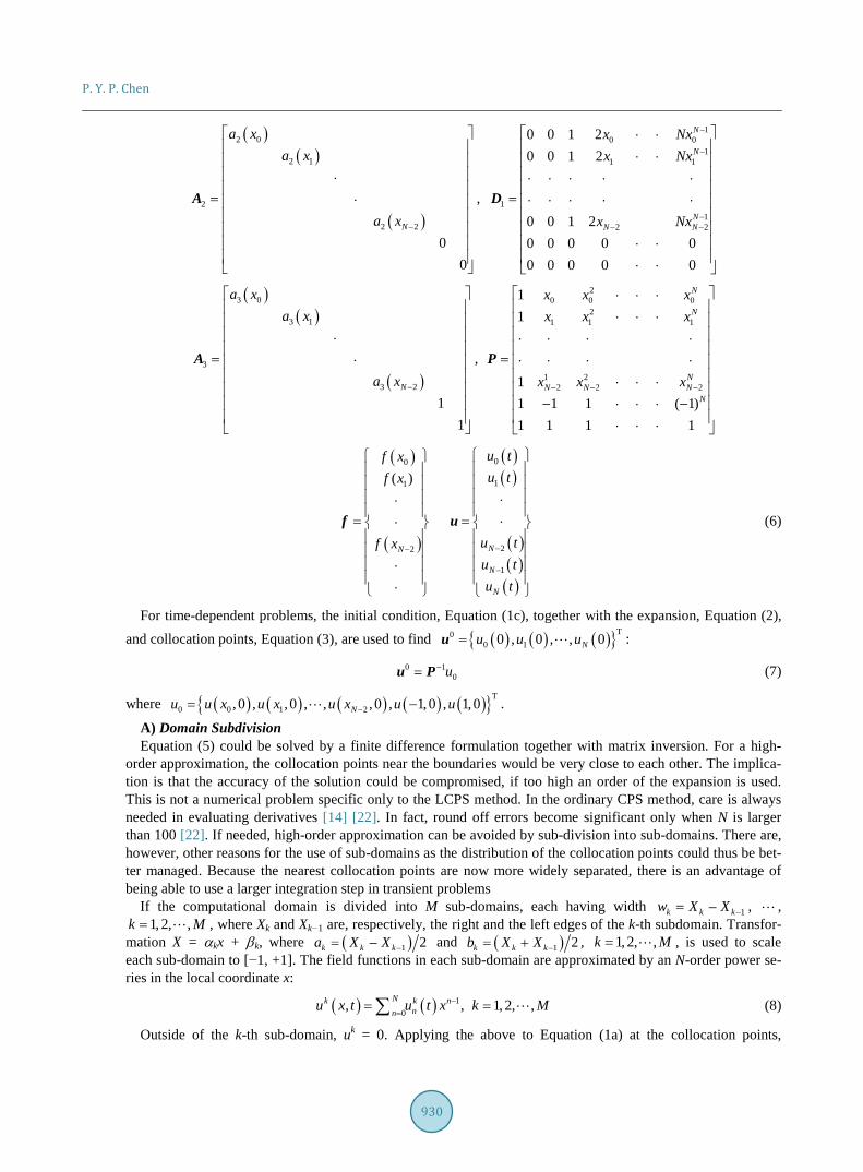
Applying the above procedure to the Equation (1a) and boundary conditions Equation (1b), results in a set of N + 1 ODEs in the form of

( ) [ ] ( )0 1 2 2 1 3d 0d

t t ft

− + + − =A u A D A D A P u (5)

where 0 10 0 00 11 1 1

00 1

2 2 2

0 0 00 0 0

N

N

NN N N

x x xx x x

x x x− − −

⋅ ⋅ ⋅ ⋅

⋅ ⋅ ⋅ ⋅ ⋅ ⋅ ⋅

= ⋅ ⋅ ⋅ ⋅ ⋅ ⋅ ⋅

⋅ ⋅ ⋅ ⋅ ⋅ ⋅ ⋅ ⋅

A .

( )( )

( )

1 0

1 1

1

1 2

00

N

a xa x

a x −

⋅

= ⋅

A ,

( )( )

( )

20

21

2

1

2

2

0

2

0 0 2 60 0 2 6

0 0 2 60 0 0 0 00 0 0

11

0 0

1

N

N

NN N

xx

x

N N xN N x

N N x

−

−

−− −

−

−

−

⋅ ⋅

⋅ ⋅ ⋅ ⋅ ⋅ ⋅ ⋅

= ⋅ ⋅ ⋅ ⋅ ⋅

⋅ ⋅ ⋅ ⋅

D

P. Y. P. Chen

930

( )( )

( )

2

2

2

2

0

1

2

00

N

a xa x

a x −

⋅

= ⋅

A ,

10

10

1

12 2

1

1

0 0 1 20 0 1 2

0 0 1 20 0 0 0 00 0 0 0 0

N

N

NN N

Nxx

xNx

Nxx

−

−

−− −

⋅ ⋅

⋅ ⋅ ⋅ ⋅ ⋅ ⋅ ⋅

= ⋅ ⋅ ⋅ ⋅ ⋅

⋅ ⋅ ⋅ ⋅

D

( )( )

( )

3

3

3

3

0

1

2

11

N

a xa x

a x −

⋅

= ⋅

A ,

20 0 0

21 1 1

1 22 2 2

11

1( 11 1 1

1 1 1 1)

N

N

NN N N

N

x x xx x x

x x x− − −

⋅ ⋅ ⋅

⋅ ⋅ ⋅ ⋅ ⋅ ⋅ ⋅

= ⋅ ⋅ ⋅ ⋅ ⋅ ⋅ ⋅

−

− ⋅ ⋅ ⋅ ⋅ ⋅ ⋅

P

( )

( )

( )( )

( )( )( )

00

11

22

1

( )

NN

N

N

u tf xu tf x

u tf xu tu t

−−

−

⋅⋅

= = ⋅⋅ ⋅ ⋅

f u (6)

For time-dependent problems, the initial condition, Equation (1c), together with the expansion, Equation (2), and collocation points, Equation (3), are used to find ( ) ( ) ( ){ }T0

0 10 , 0 , , 0Nu u u=u :

0 10u−=u P (7)

where ( ) ( ) ( ) ( ) ( ){ }T0 0 1 2, 0 , , 0 , , , 0 , 1,0 , 1,0Nu u x u x u x u u−= − .

A) Domain Subdivision Equation (5) could be solved by a finite difference formulation together with matrix inversion. For a high-

order approximation, the collocation points near the boundaries would be very close to each other. The implica-tion is that the accuracy of the solution could be compromised, if too high an order of the expansion is used. This is not a numerical problem specific only to the LCPS method. In the ordinary CPS method, care is always needed in evaluating derivatives [14] [22]. In fact, round off errors become significant only when N is larger than 100 [22]. If needed, high-order approximation can be avoided by sub-division into sub-domains. There are, however, other reasons for the use of sub-domains as the distribution of the collocation points could thus be bet-ter managed. Because the nearest collocation points are now more widely separated, there is an advantage of being able to use a larger integration step in transient problems

If the computational domain is divided into M sub-domains, each having width 1–k k kw X X −= , , 1, 2, ,k M= , where Xk and Xk−1 are, respectively, the right and the left edges of the k-th subdomain. Transfor-

mation X = αkx + βk, where ( )1– 2k k ka X X −= and ( )1 2k k kb X X −= + , 1, 2, ,k M= , is used to scale each sub-domain to [−1, +1]. The field functions in each sub-domain are approximated by an N-order power se-ries in the local coordinate x:

( ) ( ) 10

, , 1, 2, ,Nk k nnn

u x t u t x k M−=

= =∑ (8)

Outside of the k-th sub-domain, uk = 0. Applying the above to Equation (1a) at the collocation points,

P. Y. P. Chen

931

1, 2, , 1n N= − , in each sub-domain leads to the same set of equations as those for the single domain problem. The assembly of all sub-domains involves the series expansion coefficient as a vector of length ( )1N M+ × :

{ }1 1 1 2 2 20 1 0 1 0 1, , , , , , , , , , , ,M M M

N N Nu u u u u u u u u ′=u (9)

Between two adjacent sub-domains, the boundary conditions, Equation (1b), are replaced by continuity condi-tions:

1 1

1 1 1 11

d d;d d

k k k k

k kx xα α+ +

− −+

= =u u u u (10)

To implement these continuity conditions, the equations representing the boundary conditions in the matrix P in Equation (6) is changed to ones involving adjacent sub-domains as well. The matrix representing the boun-dary conditions for the k-th sub-domain are:

{ }, 1 , , 1k k k k k kS S S− + ⋅ ⋅ ⋅ ⋅ u (11)

where { }T1 1k k ku u u− += ⋅ ⋅ ⋅ ⋅u

and , 1

1 1 1 1,

0k k−

⋅ ⋅ ⋅ = ⋅ ⋅ ⋅ ⋅ ⋅ ⋅

S

( ) ( ) ( ) ( )( )

1 10

,

1 01 1 1 1 ,10 0 1 2 1

N N

k k

kN Nα

− − − ⋅ ⋅ ⋅ − − = ⋅ ⋅ −

S

( ) ( ) ( ), 1 2 1

1

2,3, , 11 0 0

,10 0 1 2 1 1 1.k k N N

kN N

k Mα

+ − −

+

⋅ ⋅ ⋅ ⋅ ⋅ ⋅ = − ⋅ ⋅ − − − =

−S

B) Selection of Collocation Points One well-discussed issue about pseudospectral methods is about collocation point selections. Other orthogon-

al polynomials, representing a set of different collocation points other than those based on the Chebyshev poly-nomials, are proposed mostly based on claims of a better accuracy. Within CPS methods, far more user are using not the roots, Equation (4) but the turning points of TN(x), known as the Gauss-Lobatto points [10] [11]. They are the roots of the polynomial ( ) ( )21 Nx T x′− , i.e.

πcos , 0jnx n NN

= − ≤ ≤

(12)

In implementation based on this selection, the first and the last of the N + 1 points are reserved for the boun-dary conditions while all other interior points are used for the collocation of the field equation. The reason for using Equation (12) is that in approximating a function, this set of collocation points will reproduced exactly the N-th order polynomial function. In general, the boundary conditions for differential equations are not always the specified functional value itself. The fact this set of collocation points could be freely used is based on the strength that spectral errors for approximating a function could easily be smaller than 10−15. For a single domain, the maximum errors will most likely be near the boundaries. With sub-domains, it is important that the selection will give the least error at cell boundaries as the inter-domain conditions include the continuity of derivatives.

3. Numerical Examples To validate the accuracy and computational efficiency of the LCPS method discussed in the previous sections, we have chosen the examples displayed below.

A) Accuracy of the Economized Chebyshev Power-Series Expansion and the Selection of Collocation Points

To test the differences between the two different choices of the collocation points, Equations (4) and (12), we use the following function:

P. Y. P. Chen

932

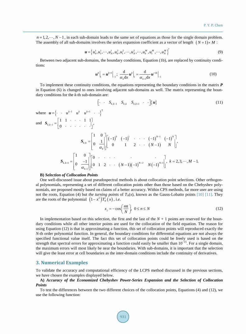
( ) ( )sech 2π 1 , 0 1f x x x= − ≤ ≤ (13)

It has been found that, at least, a 10th-order Chebyshev polynomial series is required for this function to be represented with sufficient accuracy [23]. We test the series expansion employing 9 interior collocation points, and two boundary points. We found the errors by comparing the exact functional value with those evaluated ac-cording to Equation (2), which yields exact approxe f f= − . Figure 1(a) shows that the errors at regular intervals over the complete range [0,1] are on the order of 10−3. At the exact collocation points, as shown in the plots, the errors are many orders of magnitude smaller, at 10−16. They are round-off errors, indicating that the matrix in-version is reliable. Figure 1(b) shows errors of the first derivative. From this plot, it can be seen that errors for the derivative have increased by 100-fold, as compared to the errors for the function itself. Minimum errors for the derivatives are no longer at collocation points. However, our investigation reveals that, just like in the case of the function itself, errors of the derivatives also decrease exponentially with the increasing number of the points used. Therefore, it is easy to control errors of the derivatives, although the actual number of needed points depends on the smoothness of the function and the expected accuracy, as well as the length over which the ap-proximation is made. In practice, we recommend that N ≤ 20 be used, so that the integration steps need not be very small. If more than 20 terms are required due to the necessary accuracy, the domain subdivision could be used. In this case, conditions at borders of cells include the continuity of both the function and its first derivative. We shall show in a later example that, for a multi-domain treatment, there is a clear advantage in using the set of zeros as collocation points.

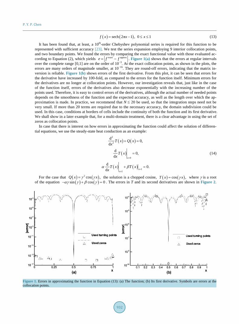
In case that there is interest on how errors in approximating the function could affect the solution of differen-tial equations, we use the steady-state heat conduction as an example:

( ) ( )2

2d 0,d

T x Q xx

+ =

( )0

d 0,d x

T xx =

= (14)

( ) ( )1

1

d 0.d x

x

T x T xx

α β=

=

+ =

For the case that ( ) ( )2 cos ,Q x xγ γ= the solution is a chopped cosine, ( ) ( )cos ,T x xγ= where γ is a root of the equation ( ) ( )sin cos 0αγ γ β γ− + = . The errors in T and its second derivatives are shown in Figure 2.

Figure 1. Errors in approximating the function in Equation (13): (a) The function; (b) Its first derivative. Symbols are errors at the collocation points.

P. Y. P. Chen

933

Figure 2. Errors in the temperature solutions obtained by the LCPS me-thod using N = 8.

It can be seen that errors in the derivatives near the boundaries are larger if the turning points are used in the collocation.

B) A Time-Independent Elliptic Equation with Material Variability In this test case the equation chosen was

( ) ( ) ( )d d , 0 1,d d

x u x f x xx xα − = < <

( ) ( )0 1 0,u u= =

( ) ( )( )sech π 2 1 ,x xα = − (15)

( ) ( )sin 2π .f x x=

This example had been used to show the flexibility and efficiency of the Chebyshev pseudospectral method [23] [25]. The analytical solution is:

( ) ( ) ( )( ) ( )( ) ( )( )21 sin 2π cosh π 1 2 1 cos 2π sinh π 1 2

8πu x x x x x = − + − − (16)

We solve this problem by rearranging Equation (15) into the same form as Equation (1), also re-scaling x into the range of [−1,1],

( ) ( ) ( ) ( )2

2d d4 , 1 1,

ddx x u x f x x

xxα α

′− + = − < <

( ) ( )1 1 0,u u− = =

( ) ( )sech π ,x xα = (17)

( ) ( )( )sin π 1 ,f x x= +

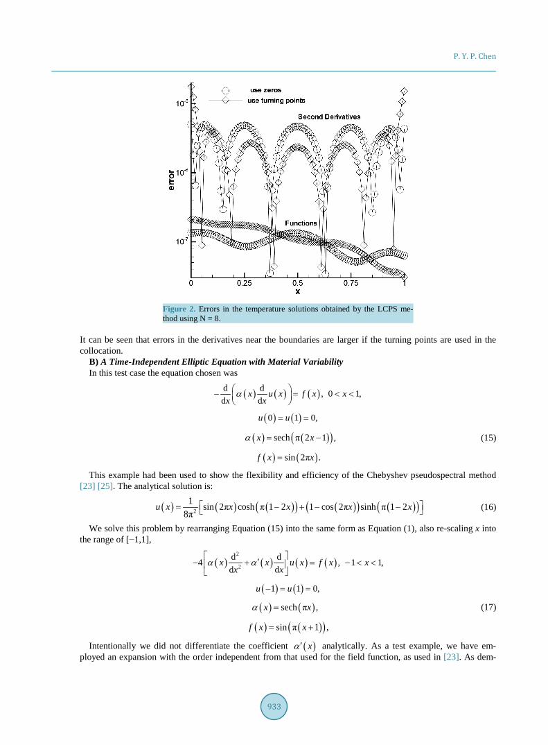
Intentionally we did not differentiate the coefficient ( )xα′ analytically. As a test example, we have em-ployed an expansion with the order independent from that used for the field function, as used in [23]. As dem-

P. Y. P. Chen

934

onstrated in Example A above, evaluating derivative α'(x) at any given point is easy with the LCPS method. There is also the freedom to choose the number of terms, so as to provide the required accuracy. Figure 3 shows our results, which are comparable in every aspect to Figure 2(a) in [11], where the CPS method was used.

C) Eigenvalues for Timoshenko beams Here we use an example that has been employed to validate the pseudospectral method for eigenvalue analy-

sis [24]. The equations for a beam with length L normalized to x∈[−1,1] are:

22

4 2 ,EI hG w hG ILL

θ α α θ ω ρ θ′′ ′+ − = −

22

22

2 2 ,

2 2 .

EI hG w hG IL L

hG hG w hwL L

θ α α θ ω ρ θ

α θ α ω ρ

′′ ′+ − = −

′ ′′− + = −

(18)

We use the particular case with clamped boundary conditions: 0, 0wθ = = (19)

For the above simultaneous equations, the LCPS method transformed them into a generalized eigenvalue problem involving matrices of size 2(N + 1) × 2(N + 1),

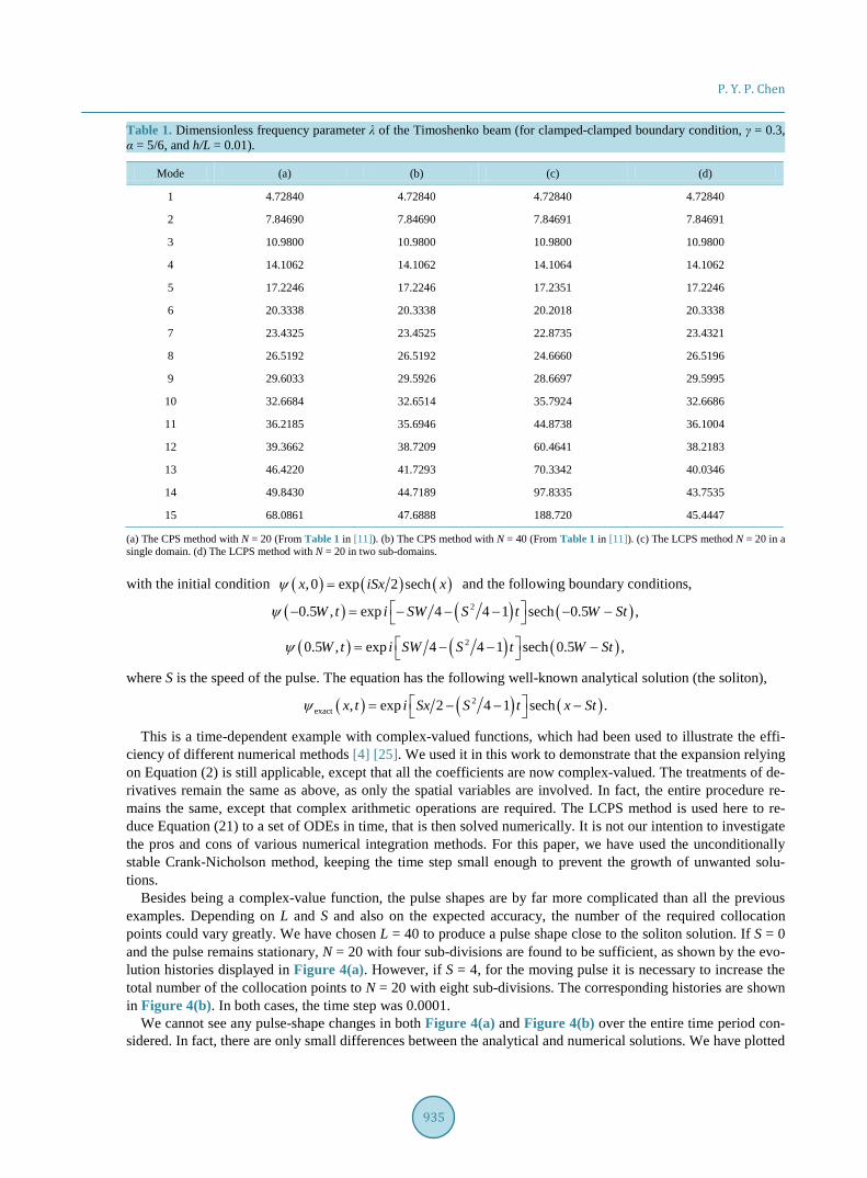
λ=Cu Du (20) where elements of the vector u are the series expansion coefficients for θ and w. We have used the general ma-trix eigenvalue solver in the IMSL package to solve Equation (20). In Table 1 we show the lowest and real di-mensionless eigenvalues found for different numbers of the collocation points, used together with results re-ported in [24]. It could be seen that all the small eigenvalues are found to be in good agreement.

D) Example of the nonlinear Schrödinger (NLS) Equation in one dimension (1D) We consider the NLS equation in 1D with a pulse width W,

[ ]22 , 0.5 ,0.5 , 0t xxi x W W tψ ψ ψ ψ= + ∈ − > (21)

Figure 3. The dependence of the solution accuracy on the number of terms used in the coefficient approximation: L is the series order of the coefficient, and N is the series order of the function.

P. Y. P. Chen

935

Table 1. Dimensionless frequency parameter λ of the Timoshenko beam (for clamped-clamped boundary condition, γ = 0.3, α = 5/6, and h/L = 0.01).

Mode (a) (b) (c) (d)

1 4.72840 4.72840 4.72840 4.72840

2 7.84690 7.84690 7.84691 7.84691

3 10.9800 10.9800 10.9800 10.9800

4 14.1062 14.1062 14.1064 14.1062

5 17.2246 17.2246 17.2351 17.2246

6 20.3338 20.3338 20.2018 20.3338

7 23.4325 23.4525 22.8735 23.4321

8 26.5192 26.5192 24.6660 26.5196

9 29.6033 29.5926 28.6697 29.5995

10 32.6684 32.6514 35.7924 32.6686

11 36.2185 35.6946 44.8738 36.1004

12 39.3662 38.7209 60.4641 38.2183

13 46.4220 41.7293 70.3342 40.0346

14 49.8430 44.7189 97.8335 43.7535

15 68.0861 47.6888 188.720 45.4447

(a) The CPS method with N = 20 (From Table 1 in [11]). (b) The CPS method with N = 40 (From Table 1 in [11]). (c) The LCPS method N = 20 in a single domain. (d) The LCPS method with N = 20 in two sub-domains. with the initial condition ( ) ( ) ( ), 0 exp 2 sechx iSx xψ = and the following boundary conditions,

( ) ( ) ( )20.5 , exp 4 4 1 sech 0.5 ,W t i SW S t W Stψ − = − − − − −

( ) ( ) ( )20.5 , exp 4 4 1 sech 0.5 ,W t i SW S t W Stψ = − − −

where S is the speed of the pulse. The equation has the following well-known analytical solution (the soliton),

( ) ( ) ( )2exact , exp 2 4 1 sech .x t i Sx S t x Stψ = − − −

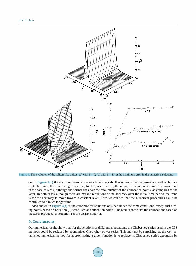
This is a time-dependent example with complex-valued functions, which had been used to illustrate the effi-ciency of different numerical methods [4] [25]. We used it in this work to demonstrate that the expansion relying on Equation (2) is still applicable, except that all the coefficients are now complex-valued. The treatments of de-rivatives remain the same as above, as only the spatial variables are involved. In fact, the entire procedure re-mains the same, except that complex arithmetic operations are required. The LCPS method is used here to re-duce Equation (21) to a set of ODEs in time, that is then solved numerically. It is not our intention to investigate the pros and cons of various numerical integration methods. For this paper, we have used the unconditionally stable Crank-Nicholson method, keeping the time step small enough to prevent the growth of unwanted solu-tions.

Besides being a complex-value function, the pulse shapes are by far more complicated than all the previous examples. Depending on L and S and also on the expected accuracy, the number of the required collocation points could vary greatly. We have chosen L = 40 to produce a pulse shape close to the soliton solution. If S = 0 and the pulse remains stationary, N = 20 with four sub-divisions are found to be sufficient, as shown by the evo-lution histories displayed in Figure 4(a). However, if S = 4, for the moving pulse it is necessary to increase the total number of the collocation points to N = 20 with eight sub-divisions. The corresponding histories are shown in Figure 4(b). In both cases, the time step was 0.0001.

We cannot see any pulse-shape changes in both Figure 4(a) and Figure 4(b) over the entire time period con-sidered. In fact, there are only small differences between the analytical and numerical solutions. We have plotted

P. Y. P. Chen

936

Figure 4. The evolution of the soliton-like pulses: (a) with S = 0; (b) with S = 4; (c) the maximum error in the numerical solutions.

out in Figure 4(c) the maximum error at various time intervals. It is obvious that the errors are well within ac-ceptable limits. It is interesting to see that, for the case of S = 0, the numerical solutions are more accurate than in the case of S = 4, although the former uses half the total number of the collocation points, as compared to the latter. In both cases, although there are marked reductions of the accuracy over the initial time period, the trend is for the accuracy to move toward a constant level. Thus we can see that the numerical procedures could be continued to a much longer time.

Also shown in Figure 4(c) is the error plot for solutions obtained under the same conditions, except that turn-ing points based on Equation (8) were used as collocation points. The results show that the collocations based on the zeros produced by Equation (4) are clearly superior.

4. Conclusions Our numerical results show that, for the solutions of differential equations, the Chebyshev series used in the CPS methods could be replaced by economized Chebyshev power series. This may not be surprising, as the well-es- tablished numerical method for approximating a given function is to replace its Chebyshev series expansion by

P. Y. P. Chen

937

its equivalent economized power-series expansion. For computational purposes, it is easier and speedier to eva-luate a power series.

Although our numerical results show that derivatives obtained from the power series are not as accurate as the function itself, this deficiency can be offset by a small increase in the order of the series used. The derivatives based on the Chebyshev economized power series retain the important property of the “spectral accuracy”. From our numerical examples, we cannot see that there are cases which could be solved by the CPS methods but can-not be solved by the LCPS method.

We have demonstrated that the formulation of the LCPS method is simpler than that for the CPS methods. It would be easier to apply the LCPS method to solve complex models. For nonlinear problems, the LCPS method will have the advantage of being able to evaluate globally and rapidly the function itself and its derivatives.

Finally, we have shown that the roots (zeros) of the Chebyshev orthogonal polynomials are better choices for the collocation points.

References [1] Canuto, C., Hussaini, M., Quarteroni, A. and Zang, T. (1988) Spectral Methods in Fluid Dynamics. Springer, Berlin.

http://dx.doi.org/10.1007/978-3-642-84108-8 [2] Gottlieb, D. and Orszag, S. (1977) Numerical Analysis of Spectral Methods: Theory and Applications. SIAM, Phila-

delphia. [3] Djidjell, K., Price, W.G., Temarel, P. and Twizell, E.H. (1998) A Linearized Implicit Pseudo-Spectral Method for Cer-

tain Non-Linear Water Wave Equations. Communications in Numerical Methods in Engineering, 14, 977-993. http://dx.doi.org/10.1002/(SICI)1099-0887(1998100)14:10<977::AID-CNM205>3.0.CO;2-T

[4] Gardner, L.R.T., Gardner, G.A., Zaki, S.I. and El Sahrawi, Z. (1993) B-Splint Finite Element Studies of the Non-Linear Schrödinger Equation. Computer Methods in Applied Mechanics and Engineering, 108, 303-318. http://dx.doi.org/10.1016/0045-7825(93)90007-K

[5] El-Daou, M.K. and Ortiz, E.L. (1994) A Recursive Formulation of Collocation in Terms of Canonical Polynomials. Computing, 52, 177-202. http://dx.doi.org/10.1007/BF02238075

[6] Liu, X. and Tai, K. (2006) Point Interpolation Collocation Method for the Solution of Partial Differential Equations. Engineering Analysis with Boundary Elements, 30, 598-609. http://dx.doi.org/10.1016/j.enganabound.2005.12.003

[7] El-Daou, M.K. and Ortiz, E.L. (1998) The Tau Method as an Analytic Tool in the Discussion of Equivalent Results across Numerical Methods. Computing, 60, 365-376. http://dx.doi.org/10.1007/BF02684381

[8] El-Daou, M.K., Ortiz, E.L. and Samara, H. (1993) A Unified Approach to the Tau Method and Chebyshev Expansion Techniques. Computers & Mathematics with Applications, 25, 73-82. http://dx.doi.org/10.1016/0898-1221(93)90145-L

[9] Ortiz, E.L. and Samara, H. (1981) An Operational Approach to the Tau Method for the Numerical Solution of Non- Linear Differential Equations. Computing, 27, 15-25. http://dx.doi.org/10.1007/BF02243435

[10] Fox, L., Ed. (1962) Numerical Solution of Ordinary and Partial Differential Equations. Pergamon, New York. [11] Lanczos, C. (1938) Trigonometric Interpolation of Empirical and Analytical Functions. Journal of Mathematical Phy-

sics, 17, 123-199. http://dx.doi.org/10.1002/sapm1938171123 [12] Luke, Y.L. (1955) Remarks on the τ-Method for the Solution of Linear Differential Equations with Rational Coeffi-

cient. Journal of the Society for Industrial and Applied Mathematics, 3, 179-191. http://dx.doi.org/10.1137/0103016 [13] Fornberg, B. (1996) A Practical Guide to Pseudo-Spectral Methods. Cambridge University Press, Cambridge.

http://dx.doi.org/10.1017/CBO9780511626357 [14] Don, W.S. and Solomonoff, A. (1995) Accuracy and Speed in Computing the Chebyshev Collocation Derivative.

SIAM Journal on Scientific Computing, 16, 1253-1268. http://dx.doi.org/10.1137/0916073 [15] Kosloff, D. and Tal-Ezer, H. (1993) A Modified Chebyshev Pseudospectral Method with an O(N-1) Time Step Re-

striction. Journal of Computational Physics, 104, 457-469. http://dx.doi.org/10.1006/jcph.1993.1044 [16] Fischer, P. and Gottlieb, D. (1997) On the Optimal Number of Subdomains for Hyperbolic Problems on Parallel Com-

puters. International Journal of High Performance Computing Applications, 11, 65-76. http://dx.doi.org/10.1177/109434209701100105

[17] Hesthaven, J.S. (1997) A Stable Penalty Method for Comressible Navier-Stokes Equations. II. One Dimensional Do-main Decomposition Schemes. SIAM Journal on Scientific Computing, 18, 658-685. http://dx.doi.org/10.1137/S1064827594276540

[18] Trefethen, L.N. (2000) Spectral Methods in Matlab. SIAM Philadelphia. http://dx.doi.org/10.1137/1.9780898719598 [19] Weideman, J.A.C. and Reddy, S.C. (2000) A MATLAB Differentiation Matrix Suite. ACM Transactions on Mathe-

P. Y. P. Chen

938

matical Software, 26, 465-519. http://dx.doi.org/10.1145/365723.365727 [20] Chen, P.Y.P. and Malomad, B.A. (2010) Single- and Multi-Peak Solitons in Two-Component Models of Metamaterials

and Photonic Crystals. Optics Communications, 283, 1598-1606. http://dx.doi.org/10.1016/j.optcom.2009.09.069 [21] Chen, P.Y.P. and Malomed, B.A. (2012) Lanczos-Chebyshev Pseudospectral Methods for Wave-Propagation Problems.

Mathematics and Computers in Simulation, 82, 1056-1068. http://dx.doi.org/10.1016/j.matcom.2011.05.013 [22] Breuer, K. and Everson, R.M. (1992) On the Error Incurred Calculating Derivatives Using Chebyshev Polynomials.

Journal of Computational Physics, 99, 56-67. http://dx.doi.org/10.1016/0021-9991(92)90274-3 [23] Seriani, D. (2004) Double-Grid Chebyshev Spectral Elements for Acoustic Wavemodeling, Wave Motion, 39, 2003.

http://dx.doi.org/10.1016/j.wavemoti.2003.12.008 [24] Lee, L. and Schult, W.W. (2004) Eigenvalue Analysis of Timoshenko Beams and Axisymmetric Mindlin Plates by the

Pseudospectral Method. Journal of Sound Vibration, 269, 609-621. http://dx.doi.org/10.1016/S0022-460X(03)00047-6 [25] Javidi, M. and Golbabai, A. (2007) Numerical Studies on Nonlinear Schrödinger Equations by Spectral Collocation

Method with Preconditioning. Journal of Mathematical Analysis and Applications, 333, 1119-1127. http://dx.doi.org/10.1016/j.jmaa.2006.12.018