the lambda cold dark matter model and cosmic...
TRANSCRIPT

The Lambda Cold Dark Matter Model and Cosmic Microwave
BackgroundKyle O’Connor
Grad Seminar 70110/28/16
1

What we will cover
• I am going to go through the LCDM model which employs the cosmological principle, uses the FLRW metric, and allows the inclusion of two free parameters in the energy densities dark energy and dark matter which are poorly understood but when included provide a good account of the evolution of the universe.
• Along the way, I will also introduce Hubble’s law and use type Ia Sn data from SDSS to calculate my own value for Hubble’s constant.
• Finally I will turn to focus on the background radiation and how it provides significant evidence that the LCDM big bang model to the universe is on the right track
2

The Big Bang
• Approximately 13.82 billion years ago the universe sprang into existence
• Expansion has been expanding ever since this moment known as the big bang
• This birth included not only that of the fabric of space‐time, but all of the matter‐energy content as well
• This matter‐energy content is broken down into ordinary (baryonic) matter, radiation, dark (non‐baryonic) matter, and dark energy
• Why do we think this?
3

A Cosmological TimelineAt the very beginning; 10 there was a period of rapid expansion to space‐time known as inflation
For the next 380,000 years the universe was so hot and dense that the radiation was constantly colliding with the electrons keeping the matter ionized as a plasma
At 380,000 years the universe had expanded enough that the universe had cooled allowing atoms to form and the photons decoupled thus forming the background radiation we see today
The first galaxies didn’t form until about 1 billion years
4

Lambda Cold Dark Matter Models ( CDM)
• This is a model of the evolution of the universe, which includes cold dark matter and dark energy
• It is often referred to as the standard model of cosmology• Two assumptions that go in to the LCDM models are that the universe, on large enough scales (~100 Mpc), is homogenous and isotropic
• Homogeneity meaning the distribution of matter is the same• Isotropy meaning that the universe looks the same in every direction • These assumptions are justified by observational data from various experiments including SDSS and WMAP (although should mention WMAP really showed that there are very tiny fluctuations in the homogeneity of the background radiation)
5

Homogenous vs Isotropic
6

Friedmann‐Lemaitre‐Robertson‐Walker Metric (FLRW metric)• This is the metric used in the LCDM model for the universe and it provides an analytic solution to Einstein’s field equations
• Each of these scientists worked out this metric and the resulting equations in the 1920’s and 1930’s independently
• This simplest model to space time geometry line element allows the spatial component to evolve with time
•Ω
• Ω sin• 1 → , k 1 → ,0 →
• is the scale factor gives the the spatial radius of curvature at some time, ,relative to the radius of curvature today, defined as 1
• is a comoving coordinate, ie a galaxy at some point is always at that same point
7
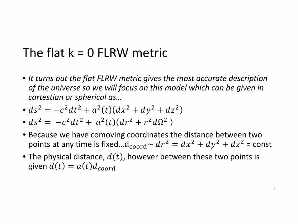
The flat k = 0 FLRW metric
• It turns out the flat FLRW metric gives the most accurate description of the universe so we will focus on this model which can be given in cartestian or spherical as…
•• Ω • Because we have comoving coordinates the distance between two points at any time is fixed…d ~ = const
• The physical distance, , however between these two points is given
8

Comoving CoordinatesNotice that the coordinate distance has not changed they are still 4
However, the physical distance between the two objects has obviously increased from 1 → 2 , such that 2 21 1
If you imagine t2 to be the present, t2 ~t0, then a(t2) ~ a(t0) = 1, then a previous time t1, at which the physical distance between two objects is half the physical distance of the present results in a(t1) = 1/2
a(t) gives the ratio of the physical distance between two objects at some time t to the physical distance at the present
9

Cosmological RedshiftThe cosmological redshift is the Doppler effect from expanding space rather than relative velocities of two objects
Any light in the universe is stretched as it travels such that the wavelength observed, , is different from the wavelength when
emitted, , and can be related to the scale factors at the time of emission, , and at observation, , by the relation
1 /
The term z here is given the name cosmological redshift
10

Hubble’s Law
• If you take the time derivative of the relation between proper distance and the scale factor we obtain Hubble’s Law
• ∴• This can be rewritten as
•• For nearby galaxies ≪ the redshift may be written using Hubble’s constant, the value of the hubble parameter at the present,
~ •
11

Sloan Digital Sky Survey (SDSS)Using a ground based telescope in New Mexico the redshifts of distant objects are measured
This experiment provides a map giving locations and redshifts to more than 1/3 of the sky
From this data it is determined that on average the distribution of galaxies is homogenous and isotropic on length scales ~ 100 Mpc
Using the type Ia Sn data from the SDSS I made a Hubble diagram which plots the redshift of nearby supernovae versus their distance to determine a value for Hubble’s constant, the current rate of expansion of the universe
12
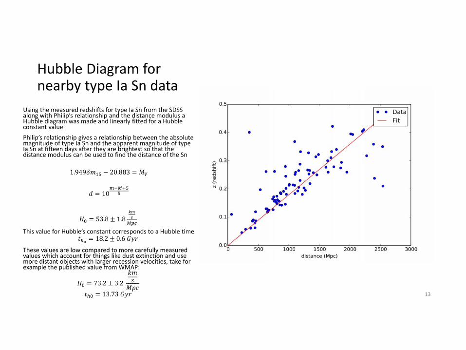
Hubble Diagram for nearby type Ia Sn data
Using the measured redshifts for type Ia Sn from the SDSS along with Philip’s relationship and the distance modulus a Hubble diagram was made and linearly fitted for a Hubble constant valuePhilip’s relationship gives a relationship between the absolute magnitude of type Ia Sn and the apparent magnitude of type Ia Sn at fifteen days after they are brightest so that the distance modulus can be used to find the distance of the Sn
1.949 20.883
10
53.8 1.8
This value for Hubble’s constant corresponds to a Hubble time18.2 0.6
These values are low compared to more carefully measured values which account for things like dust extinction and use more distant objects with larger recession velocities, take for example the published value from WMAP:
73.2 3.2 13.73 13

Energy densities
• Allow , , to represent the energy densities of matter, radiation, and the vacuum energy in our universe
• These energy densities can be shown to change with the scale factor using the first law of thermodynamics
• is the change in energy for a particular source of energy, is heat added to the system, is work done on the system
• For our homogenous isotropic universe, there can be no heat flow so 0 and we get
• The work done can be represented as • is the pressure on the walls of the system, it is negative because that energy would go into changing the volume of the system, is the change in volume of the universe
•
14

Energy Densities• Allow , , to represent the energy densities of matter, radiation,
and the vacuum energy in our universe
• These energy densities can be shown to change with the scale factor using the first law of thermodynamics
• is an infinitesimal change in energy for a particular source of energy, is the infinitesimal heat added to the system, d is the infinitesimal work done on the system from outside
• For our homogenous isotropic universe, there can be no heat flow so 0
• The infinitesimal change in energy is the same as the energy density at that time and the infinitesimal change in volume
• The infinitesimal work done is completely from the source, since there is nothing external from the universe, it is related to the pressure and the infinitesimal volume change
• is the pressure on the walls of the system, it is negative because that energy would go into changing the volume of the system,
is the change in volume of the universe
• In the last expression I pulled out the constant and divided by to find the time rate of change for the energy density in terms of
the pressure from that source and the scale factor
• d dW
• ; dW pd ;
•
15

• Since the matter in the universe is well approximated to be a pressure less gas, and we will assume mass is neither created or destroyed, the first law for the matter in the universe becomes:
• 0 ⇒ 0
• This is intuitive if you consider a simple case, the mass isn’t changing so the energy density at some time earlier say for example when the universe was half its current size the volume decreases by factor of eight such that the energy density of the matter at the earlier time increases by the same factor of eight
16

• To determine how the energy density of the background radiation changes with the scale factor, recall the effect the cosmological redshift has on lowering the frequency and thus energy of this radiation in expanding space
• Also use again the assumption that the amount of this radiation is not changing
• Lastly the temperature of this blackbody radiation can be related to the energy using the Stefan‐Boltzmann law ∝to find the temperature of empty space at earlier times in terms of the scale factor
• 0
• 0
• 0
• 0 7.1 ∗ 10 / ^3• 0 2.7
17

• The energy density of the vacuum i.e. dark energy is constant
• The universe is currently in a phase of vacuum energy domination
• If you plot these energy densities against the scale factor using the measured values of the current energy densities you can see when the universe transitions from one phase to the next
• 10
18

Phases of the universeThis plot was made using the current day values of the energy densities measured by WMAP in , and the relations of the energy densities to the scale factor
The intersection between the matter energy density curve and dark energy density curve occurs at a scale factor value corresponding to a time of approximately
after the big bang
The intersection between the radiation energy density curve and matter energy density curve occurs at a scale factor value
corresponding to a time of approximately after the big bang
19

The Universe’s Energy Density Content The fractional energy densities of the universe changes as the universe expands
The radiation has an energy inversely proportional to its wavelength / This wavelength gets stretched as the universe expands; thus the energy density of radiation drops
The matter energy content is constant since the amount of mass isn’t changing, however the matter energy density also drops since it is inversely proportional to the volume of the universe
The radiation energy density is dropping at a faster rate than the matter energy density
The moment they crossed and the universe entered into a matter‐dominated era was when the radiation decoupled as atoms began to form
We are currently in the dark energy dominated era (as of 9.4 gyr)
20

Einstein’s Field Equations
• Λ• is the Einstein tensor which consists of the Ricci curvature tensor,
, the metric tensor, , and the scalar curvature it basically describes how the spacetime is curved
• is the stress‐energy tensor describes the distribution of matter/energy it is like the source of the gravitational field
• Λis the cosmological constant or vacuum energy term which is causing expansion; originally omitted by Einstein
•• The metric tensor, , and the energy momentum tensor, , need to be determined and plugged in to obtain the set of equations from this tensor equation
21

The Friedmann Equations• When using the FLRW metric and perfect fluid stress energy tensor to solve the Einstein equations one obtains two non‐trivial equations
•
•• The solution to these equations give us the proportionalities of the scale factor with respect to time for the different phases of the universe
• In the early radiation dominated universe ∝• In the matter dominated universe ∝• In the vacuum dominated universe ∝• As you can see the rates of expansion for the different phases are different; they all expand, but taking the time derivatives you see that for the matter dominated and radiation dominated we have the rate of expansion slowing down while the vacuum dominated expansion would be accelerating
22

Critical Density and relative energy densities • The critical density is defined as the total present energy density in a flat FLRW model (while ignoring the cosmological constant term)
• If we evaluate the first FLRW equation at the present and divide by the current scale factor squared we get a connection to the critical density and Hubble’s constant
• 10• For our flat model we can get fractional values for the different energy densities relative to the critical density in our flat model the sum of which must be one
• Ω 1 Ω Ω Ω
23

WMAP’s Relative Energy Densities (Current)
• The relative energy densities today are:
• Ω 71.4%• Ω 24%• Ω 4.6%• The relative energy density of the background radiation is negligibly small today
• Also note the separation of baryonic matter and cold dark matter
24

Summary to the LCDMThe LCDM model makes several predictions that have been corroborated by experiment
The large scale structure of the CMB and galaxies (really were assumptions that went into the model) but this too has been verified by observation
The current accelerated expansion of the universe; this is verified by astronomers using type Ia Sn light curves
It also predicts the abundance of elements in the universe provided a value for the abundance of ordinary matter, by mass we have Hydrogen ~ 75%, Helium ~24% and heavier elements taking up 1%, The WMAP theoretical results using their observed abundance of ordinary matter agree in this model agree very well with the actual observed abundances of the elements
25

The background radiation • What I would like to talk about now is the background radiation, all that radiation leftover from the initial moment of the big bang
• It is referred to as the microwave background because that is the part of the spectrum in which it is most visible today with a wavelength of approximately 7.4 cm
• Although negligible in terms of its present contribution to the total energy density of the universe, its detection and study of its near but not perfect uniformity is perhaps the strongest support to the legitimacy of the big bang and LCDM model
• This background radiation separated from the early universe plasma at a time of about 380,000 years after the big bang
• At the moment of decoupling the radiation was at a temperature of about 3000 K and the universe went from opaque to transparent
• The reason for this decoupling was free electrons had finally cooled enough to join with protons to form Hydrogen atoms and the number of free electrons for the radiation to scatter from dropped significantly
• This increased the mean free path for the radiation and it was able to separate from the early universe plasma
26
The theoretical foundation and accidental discovery• The cosmic microwave background was first theorized by George Gamow a Ukrainian‐American Physicist in the 1940’s following the big bang theory; he estimated that it would be at a temperature of 50K
• In the following years others including Robert Dicke, Ralph Alpher, Robert Herman, all published papers with various predictions of this same background radiation with estimates of the temperature varying between 5K ‐> 50K
• In the 1960’s just when it was determined that this radiation would be detectable and plans were getting underway to set up experiments two workers Arno Penzias and Robert Wilson working at Bell Labs accidentally discovered the CMB
27

How de we know it is actually there?
The first direct evidence for the CMB comes from Arno Penzias and Robert Wilson who were working at a very sensitive antennae to detect radio waves at the Bell Labs in New Jersey in 1964 These radio waves they were detecting were supposed to be reflections of a signal reflected off an Echo satellite in orbit around EarthAfter carefully removing all known interference they noticed a constant noise with wavelength approximately 7 cmThis noise turned out to be the first direct evidence of the CMB and won them the Nobel Prize in 1978
28

Echo Program• The echo satellite which was used to bounce signals sent from N.A.S.A Jet Propulsion lab to the Bell Labs Receiver
• After exhausting methods to eliminate the noise at receiver, aside from what was expected to be received by balloon reflection, they found it to be constant and independent of direction and time of day and year
• They also were put in touch with Robert Dicke, one of the scientists working on observing this radiation at the time
• It was thus determined this noise was not from Earth the Sun or our galaxy; it was the CMB measured by them with temperature about T = 3.5 K
29

An opaque universe plasma
• The horizon distance is the maximum distance a particle could have traveled to an observer in the current age of the universe
• Today the horizon distance is 14.0 45.7• It is the radius from our spot, or any other spot, of the observable universe in all directions is 45.7 Gly
• The decoupling of the background radiation occurred when the horizon distance was equal to the mean free path of the photons
• The photons on average could travel this maximum distance without an interaction
30

Decoupling and the Rate of Compton Scattering• The universe was opaque while it was still a plasma since photons were constantly being scattered by the matter not being allowed to “escape” off on their own path away from the matter since they won’t be absorbed except at certain spectral wavelengths once atoms have formed and interactions become much less frequent with less free electrons
• The wavelength of the radiation was shorter than the mean free path between collisions with matter
• The universe became transparent once atoms formed because the photons then began to travel away from the matter and out across the entire universe; This is the earliest point we can possibly see back to before this moment light did not travel outside of the plasma
31

An AnalogyThe reason we can’t see earlier than the decoupling is that all of the light from before this moment is absorbed or scattered inside the plasma none is scattered away towards us similar to how light from the sun on a cloudy day we see the cloud and the rest of the sky behind it is blocked because the light was scattered last from the cloud towards us
32

COBE Spectrum Data The emission spectrum for the background shows that it is most intense around a wavelength of about 1mm this is in the microwave part of electromagnetic spectrum hence microwave background
The fit curve shows the spectrum that would be expected for an ideal black body in thermal equilibrium at T ~ 2.73 K
The black body spectrum is a nearly perfect fit to the data, more evidence to the homogeneity for the thermal equilibrium
Subsequent tests such as WMAP and Planck showed these same sort of agreements with much higher levels of precision though which do in fact show very small fluctuation and anisotropy
33

The background radiation fluctuationsThese maps show the fluctuations of the temperature of the background radiation
It takes the galaxy foreground, dipole anisotropy and average background temperature and subtracts it out from the measurements leaving just the residuals in the background temperature data
These fluctuations are very small at the part per million level
It is easily noticed that the precision increases with each experiment as the angular resolution is improved
34

The scale of the fluctuationsIn these temperature maps red is hot,blue is cold, green is average. The plane of the milky way is through the horizontal center of the ellipse If you look at the temperature maps for the data from COBE and WMAP using different temperature intervals between hot and cold you don’t notice any anisotropy until you have set the scale to very small deviations from average on the order of ~ 4 ∗ 10
Even at this scale however the anisotropy is a “false” anisotropy (it doesn’t arise from the deviation among the cmb fluctuations) termed as dipole anisotropy which due to the movement of the milky way relative to the observed background, where we move away it seems cooler where we moving towards it seems warmer The true deviations after subtracting this dipole anisotropy don’t show up until we are an order of magnitude smaller at ~ 1 ∗ 10
35

Importance of the small fluctuations
• If there were no fluctuations in the CMB that would mean that our assumption that the universe was completely homogenous and isotropic in the LCDM model was correct
• However this would also mean no large scale structures like galaxies or stars would ever have formed since the pull would be the same from gravity in each direction, matter would never have clumped together
• These small fluctuations in the distribution of matter arose during the period of inflation and the evidence we see of the small fluctuations in the background lends support to the theory of inflation
36

Conclusions/Take home points
• The vacuum energy a form of energy we have little to no understanding of consists of approximately 72% of todays current energy density
• Cold dark matter another form of energy we have little physical understanding of what it is besides modeling how it might be distributed and how it interacts gravitationally in solving questions such as the galaxy rotation problem takes up 23% of the current energy density
• Baryonic matter takes up only approximately 4.6% of the current energy density
• The LCDM model allowing these parameters to be included along with cosmological principle assumption makes predictions for the H:HE ratio which match current observational data, predicts existence and structure of CMB which is verified by various experiments, and predicts the current accelerated expansion which has also been verified
37
Questions?/Sources
• https://map.gsfc.nasa.gov/WMAP
• http://www.sdss.org/ SDSS• http://arxiv.org/abs/1103.2976Riess Paper for his H0
• Hartle, James, Intro to GR • Wikipedia
38