the labrador sea deep convection experiment -...

2033Bulletin of the American Meteorological Society

*The Lab Sea Group:J. Marshall, Massachusetts Institute of Technology, Cambridge,Massachusetts.F. Dobson, Bedford Institute of Oceanography, Dartmouth, NovaScotia, Canada.K. Moore, University of Toronto, Toronto, Canada.P. Rhines, University of Washington, Seattle, Washington.M. Visbeck, Lamont-Doherty Earth Observatory, Palisades, NewYork.E. d’Asaro, Department of Meteorology, University of Washing-ton, Seattle, Washington.K. Bumke, Department of Meteorology, Institut für Meereskunde,University of Kiel, Kiel, Germany.S. Chang, Naval Research Laboratory, Monterey, California.R. Davis, Scripps Institution of Oceanography, San Diego, Cali-fornia.K. Fischer, Environmental Research Institute of Michigan, AnnArbor, Michigan.R. Garwood, Naval Postgraduate School, Monterey, California.P. Guest, Naval Postgraduate School, Monterey, California.R. Harcourt, Naval Postgraduate School, Monterey, California.C. Herbaut, Massachusetts Institute of Technology, Cambridge,Massachusetts.

T. Holt, Naval Research Laboratory, Monterey, California.J. Lazier, Bedford Institute of Oceanography, Dartmouth, NovaScotia, Canada.S. Legg, Woods Hole Oceanographic Institution, Woods Hole,Massachusetts.J. McWilliams, University of California, Los Angeles, Los An-geles, California.R. Pickart, Woods Hole Oceanographic Institution, Woods Hole,Massachusetts.M. Prater, University of Rhode Island, Kingston, Rhode Island.I. Renfrew, University of Toronto, Toronto, Canada.F. Schott, Department of Meteorology, Institut für Meereskunde,University of Kiel, Kiel, Germany.U. Send, Department of Meteorology, Institut für Meereskunde,University of Kiel, Kiel, Germany.W. Smethie, Lamont-Doherty Earth Observatory, Palisades, NewYork.Corresponding author address: Dr. John Marshall, Bldg. 54-1256,Department of Earth, Atmosphere, and Planetary Studies, Mas-sachusetts Institute of Technology, Cambridge, MA 02139.E-mail: [email protected] final form 24 July 1998.©1998 American Meteorological Society

The Labrador Sea DeepConvection Experiment

The Lab Sea Group*

ABSTRACT

In the autumn of 1996 the field component of an experiment designed to observe water mass transformation beganin the Labrador Sea. Intense observations of ocean convection were taken in the following two winters. The purpose ofthe experiment was, by a combination of meteorological and oceanographic field observations, laboratory studies, theory,and modeling, to improve understanding of the convective process in the ocean and its representation in models. Thedataset that has been gathered far exceeds previous efforts to observe the convective process anywhere in the ocean,both in its scope and range of techniques deployed. Combined with a comprehensive set of meteorological and air–seaflux measurements, it is giving unprecedented insights into the dynamics and thermodynamics of a closely coupled,semienclosed system known to have direct influence on the processes that control global climate.

1. Introduction

a. Meteorology and oceanography of the LabradorSeaThe northwest corner of the Atlantic Ocean (the

Labrador Sea sketched in Fig. 1) is a region of power-ful physical forces, extremes of wind and cold, incur-

sions of icebergs and sea ice, great contrasts in buoy-ancy of air and seawater, and a region of great biologicalactivity. Intense air–sea interaction occurs here withstrong upward heat flux at the sea surface. The proxim-ity of the region to the principal North Atlantic stormtrack of the atmosphere results in a strong modulationof air–sea interaction by passing extratropical cyclones.

2034 Vol. 79, No. 10, October 1998

The response of the Labrador Sea involves a fun-damental fluid dynamical process: buoyancy-drivenconvection on a rapidly rotating planet. Heat loss fromthe ocean is induced by cyclonic atmospheric circula-tion over the North Atlantic in winter, which advectscold, dry arctic air over the relatively warm (~2°C)waters of the Labrador Sea. Peak heat losses in wintercan reach many hundreds of watts per square meter(G. Moore et al. 1998, manuscript submitted to J. Cli-mate, hereafter MAH; I. Renfrew and G. Moore 1998,manuscript submitted to Mon. Wea. Rev.) and the re-sultant buoyancy loss causes the surface waters of the

ocean to sink. But because the fluid isstiffened by the earth’s rotation, sinkingof the cooled water compresses “Taylorcolumns,” generating strong horizontalcirculation. The heat lost from the oceanis taken up by the atmosphere, which alsoresponds in a convective manner. But be-cause the timescale of response in the at-mosphere is so much shorter, here rotationis not an important constraint on the mo-tion. As a result, the convection that occursover the Labrador Sea has a very differ-ent manifestation from that which occursin it, often being organized in a quasi-lin-ear manner that results in roll clouds thatare a ubiquitous feature in satellite imagesof the region (e.g., see Fig. 2). However,atmospheric convection is tied to the to-pography of the basin and thus affects thepattern of surface buoyancy fluxes; it isvery much part of the coupled problem.

The important convection, climate,and circulation of the Labrador Sea, tobe described further below, encouragedus to follow the historic lead of earlierCanadian initiatives and develop a mul-ticomponent program of observationsand modeling. Prompted by simulationsof rotating convection on the computer(e.g., Jones and Marshall 1993) and inthe laboratory (e.g., Maxworthy andNarimousa 1994) and by the establish-ment of a National Oceanic and Atmo-spheric Association (NOAA)-fundedtime series mooring in the central Labra-dor Sea, the U.S. Office of Naval Re-search formed the Accelerated ResearchInitiative on Oceanic Deep Convection.

The deep convection experiment,whose field program began in the autumn of 1996, hasas its primary focus the oceanic convective process andits interaction with geostrophic and basin-scale eddiesand circulation. But its proximate goals have grownto be major efforts in themselves: the investigation ofthe atmospheric, synoptic, and mesoscale dynamicsthat result in intense air–sea interaction in the region;the coupled dynamics of the deep convection processin the atmosphere and ocean; the communication ofnewly convected waters of the Labrador Sea with theWorld Ocean; and the relation between convection anddecadal climate variability.

FIG. 1. Schematic showing the cyclonic circulation and preconditioning of theLabrador Sea. The typical depth of the σ = 27.6 isopycnal in the early winter is con-toured in meters. The warm circulation branches of the North Atlantic Current andIrminger sea water (ISW) and the near-surface, cold, and fresh East/WestGreenland and Labrador Currents are also indicated. (From Marshall and Shott 1998.)


The experiment took place,quite fortuitously, in the largercontext of the Frontal and Atlan-tic Storm-track Experiment(FASTEX) and the validationprogram for the National Aero-nautics and Space Administra-tion (NASA) scatterometer onthe Advanced Earth ObservingSatellite. The FASTEX goalswere to investigate, with a newrange of forecast models, the de-velopment and evolution of low-pressure systems over the NorthAtlantic Ocean (see Joly et al.1997). We also benefited by thelarge-scale oceanographic de-scription provided by interna-tional efforts organized by theWorld Ocean Circulation Ex-periment (WOCE) in the Atlan-tic Ocean. The context providedby these related experimentswill provide a much clearer andmore complete picture of thesynoptic meteorology and ambi-ent oceanographic conditionsthat occurred in the LabradorSea and its environs.

Advanced and newly con-ceived technologies abound inthe Labrador Sea experiment;beyond classic hydrographicsections and moorings measuring velocity, salinity,and temperature, we deployed drifting and profilingfloats; three-dimensional nearly Lagrangian driftersthat can follow the convective process vertically aswell as horizontally; acoustic tomography and verti-cal echo sounding aimed at long-baseline temperature,salinity, and currents; newly designed conductivity–temperature–depth profiler (CTD) moorings, andmoored and lowered acoustic Doppler currentprofilers; shipboard air–sea flux instrumentation; waveradar systems; airborne and satellite passive micro-wave and scatterometer systems; and synthetic aper-ture radars. In the second season of field work,1997–98, autonomous underwater vehicles were alsodeployed to map fine structure in the boundary layer.The datasets that have been and are being gathered farexceed previous efforts to observe the convective pro-cess anywhere in the ocean, both in the scope and range

of techniques deployed. We are now in a position totest new theoretical ideas, the fidelity of ocean gen-eral circulation models, parameterizations of convec-tive mixing, and to explore new and exciting scientificterritory.

Here we give an overview of the important scien-tific issues that are being addressed by the experimentand provide a preliminary description of results fromthe field work. The paper is set out as follows. After astatement of the major aims of the experiment, we dis-cuss the circulation and climatological context inwhich it is being carried out and some of the theoreti-cal and modeling issues that motivate it in section 2.The planning of the multifaceted experiment is dis-cussed in section 3 and some of our preliminary find-ings in section 4. Finally, conclusions and the futureoutlook are presented in section 5.

FIG. 2. Infrared advanced very high resolution radiometer image from the NOAA-14 po-lar orbiter at 1141 UTC on 7 February 1997 showing an extratropical cyclone over the NorthAtlantic. The location of the low pressure center is indicated by the L. The bright and there-fore high clouds to the north of the low pressure center are associated with the system’swarm sector. The less bright and therefore shallow clouds to the east of the low, organizedinto quasi-two-dimensional bands, are associated with the northwesterly flow that results inthe advection of cold and dry polar air over the Labrador Sea.

2036 Vol. 79, No. 10, October 1998

b. Aims of the experimentMany of the details of the water mass transforma-

tion process in the ocean remain largely unknown be-cause they are difficult to observe and model. Theoverarching goal of the Labrador Sea Convection Ex-periment (LSCE) is then to improve our understand-ing of the convective process in the ocean, and hencethe fidelity of its parametric representation in large-scale ocean models, through a combination of meteo-rological and oceanographic field observations,laboratory studies, theory, and modeling.

The water mass transformation process in theocean is inherently complicated, involving air–seainteraction and the interplay of a hierarchy of oceanicscales: convective plumes (on scales of order 1 km)that act to homogenize properties to form a “mixedpatch,” eddies that orchestrate “lateral exchange” be-tween the mixed patch and the ambient fluid throughadvective processes (on a scale of a few tens of kilo-meters), and the large-scale circulation itself (overhundreds of kilometers) involving the ocean gyre andboundary currents. The scales of the key phenomenonare represented schematically in Fig. 3.

Our modeling and observational strategies were de-signed to address each of the scales and its interactionin the context of the prevailing meteorological forc-ing that drives the whole process in the depths of win-ter. The key oceanographic and meteorologicalobjectives are outlined below.

1) OCEAN

The objectives at each of the oceanographic scalesare as follows.

• Plume scale (100 m–1 km): Determine the char-acteristic scales, properties, and integral fluxes ofa population of convective plumes and how theydepend on the atmospheric forcing and their localenvironment.

• Eddy scale (5 km–100 km): Understand how theconvective process is related to and organized byits large-scale environment and the relative impor-tance of balanced (geostrophic) versus unbalanced(nonhydrostatic) processes in the flux of heat andsalt both laterally and vertically.

• Gyre scale (50–1000 km): Determine the large-scale factors that control the volume and tempera-ture/salinity (T/S) properties of the convectivelycreated water masses and how they are subse-quently accommodated into the general circulationof the ocean; describe the mean and seasonal varia-

tion in the circulation of the Labrador sea.

2) ATMOSPHERE

The aims of the meteorological component of theexperiment are to

• understand the physics of the atmospheric pro-cesses in the Labrador Sea that force oceanic mix-ing and deep convection;

• collect a set of high quality in situ surface fluxesof heat, fresh water, radiation, and momentum inconditions representative of those in which deepconvection occurs;

• use the in situ measurements to “test” remotelysensed products; and

• use the in situ measurements to assess the abilityof atmospheric numerical models to correctly rep-resent the air–sea interaction that occurs in the re-gion and, where needed, improve the boundarylayer parameterization in these models so as to bet-ter represent the interaction.

2. Background

a. The Labrador SeaThe weak density stratification of the Labrador Sea

is broken down each wintertime, recently to depthsgreater than 2000 m, making it one of the most extremeocean convection sites in the World Ocean. A lens-shaped water mass (Labrador sea water, or LSW) of

FIG. 3. Scales of phenomena involved in deep convection: themixed patch on the preconditioned scale created by convectiveplumes and geostrophic eddies that orchestrate the exchange offluid and properties between the mixed patch and the stratifiedfluid associated with the peripheral boundary current.


dimension 500 km × 700 km × 2 km deep has devel-oped in response to this wintertime air–sea heat flux(Fig. 4). It is weakly stratified, with a temperature near2.8°C, a salinity of 34.83 ppt, and a potential densityof 27.78 kg m−3. Deep convective cooling to the atmo-sphere competes with the buoyant, low-salinity near-surface waters nearby and with the warmth of thesubtropical waters just beneath the surface. The neteffect on the oceanic general circulation is to transportsalt and heat poleward in the surface layers and low-salinity, cooled waters southward to the rest of theWorld Ocean at depths between 1 and 2 km, produc-ing fresh new deep water on a quasi-continuous ba-sis, with all the climate implications of such aproduction. The Labrador Sea is also an importantcomponent of the “thermohaline circulation,” the glo-bal meridional-overturning circulation that is respon-sible for roughly half of the poleward heat transportdemanded by the atmosphere–ocean system.

Figure 5 shows the average mean sea level pres-sure, 10-m wind, and total heat flux fields for all win-ter months during the period from 1968 to 1997, asdetermined by the National Centers for Environmen-tal Prediction–National Center for Atmospheric Re-search (NCEP–NCAR) Reanalysis Project (Kalnayet al. 1996). Note in this context a winter is definedas the months of December, January, February, andMarch. One can see that in winter the North Atlanticis under the influence of the Icelandic low and theAzores high. Thus one would expect cyclonic flowover the North Atlantic associated with the movementof synoptic-scale weather systems along a track fromthe eastern seaboard of North America to Iceland. This“mean” cyclonic circulation overthe North Atlantic results in the ad-vection of cold and dry arctic air overthe relatively warm waters (~2°C)of the Labrador Sea, resulting in alarge transfer of heat from the oceanto the atmosphere as shown in Fig. 5.In the center of the Labrador Sea, theaverage winter heat loss exceeds300 W m−2, a value that is of the sameorder of magnitude as that which oc-curs in the temperate Sargasso Sea tothe east of the Gulf Stream. Althoughaveraging tends to blur spatial gra-dients, the highest heat loss in theLabrador Sea occurs in an ellipticalregion some 150 km wide situatedalong the Labrador coast just off the

sea–ice edge where peak values can exceed1000 W m−2.

The surface waters of the Labrador Sea are suffi-ciently warm, except near the sea–ice margin, thattheir contraction under cooling can cause convectiveoverturning. The delicate balance of the cold and freshwater from continental runoff and sea–ice melt, andthe inflow of the warm and salty water of the IrmingerCurrent (see Fig. 1) maintains the temperature andsalinity of the surface waters at elevated values.

In addition to the large uncertainty that exists withregard to the spatial and temporal variability in the air–sea flux in the region, the equally important freshwa-ter cycle has received much less attention. Theprecipitation-induced supply of buoyancy to the sur-face waters of the Labrador Sea can have a direct im-

FIG. 4. Autumn hydrographic section of potential temperature(October 1996) along AR7 (marked in Fig. 1) showing the lens-shaped bolus of Labrador Sea water extending down to about2 km, formed by convection in previous winters (courtesy ofA. Clarke and J. Lazier).

FIG. 5. Average mean sea level pressure (contour, mb), 10-m wind (vector, m s−1),and total heat flux (color scale, W m−2) fields from the NCEP–NCAR Reanalysisover all winter months (December, January, February, March) during the period1968–97.

2038 Vol. 79, No. 10, October 1998

pact on the convective process in the ocean (MAH).Supply through river runoff, freshwater release in icemelt as well as advection by ocean currents are allimportant in the buoyancy budget. Direct measure-ments show significant (> 1 Sverdrup) inflow from theArctic through the Davis Strait, as well as input via theEast Greenland Current. The freshwater runoff fromCanada is also very great, evident for example in thehigh tritium concentration of surface waters (tritium thatis locked up in continental ground water and ice is rela-tively undiluted, compared with ocean-borne tritium).

THE CONVECTIVE PROCESS

Observations suggest that there are certain recur-ring features and conditions that predispose a regionto deep-reaching convection and that are common toall known sites of deep convection—the Mediterra-nean, Greenland, and Labrador seas (e.g., see Marshalland Schott 1998). First, there must be strong atmo-spheric forcing due to thermal and/or haline surfacefluxes. Thus open ocean regions adjacent to bound-aries are favored, where cold and dry winds from landor ice surfaces blow over water inducing large sensibleand latent heat and moisture fluxes. Second, thestratification beneath the surface mixed layer must beweak, made weak perhaps by previous convection.And third, the weakly stratified underlying watersmust be brought up toward the surface so that they canbe readily and directly exposed to intense surface forc-ing. This latter condition is favored by cyclonic cir-culation associated with density surfaces that “domeup” to the surface. All these conditions are readily sat-isfied in the Labrador Sea (see Fig. 1).

Since the classic MEDOC experiment in the Medi-terranean (MEDOC Group 1969) three phases ofocean convection have been identified (sketched sche-matically in Fig. 6) and provide a useful contextto consider the convective process in the Labrador Sea(see Clarke and Gascard 1983): “preconditioning”on the large scale (of order 100 km), “deep convec-tion” occurring in localized, intense plumes (on scalesof order 1 km), and lateral exchange between theconvection site and its surroundings. The last twophases are not necessarily sequential and often occurconcurrently.

During preconditioning (Fig. 6, panel I), the gyre-scale cyclonic circulation and buoyancy forcing typi-cal of the convection site predispose it to overturn.Subsequent cooling events may then initiate deep con-vection in which a substantial part of the fluid columnmay overturn in numerous plumes (Fig. 6, panel II)

that distribute the dense surface water in the vertical.The plumes are thought to have a horizontal scale ofthe order of their lateral scale, ~1 km, with vertical ve-locities of up to 10 cm s−1. They mix properties overthe preconditioned site, forming a homogeneous deepmixed patch ranging in scale from several tens to per-haps many hundreds of kilometers in diameter. Withthe cessation of strong forcing, the predominantly ver-tical heat transfer due to convection gives way to hori-zontal transfer associated with eddying on geostrophicscales. The mixed fluid disperses under the influenceof gravity and rotation, spreading out at its neutrallybuoyant level, leading, on a timescale of weeks, to thedisintegration of the mixed patch and reoccupation ofthe convection site by the stratified fluid of the periph-ery (Fig. 6, panel III).

The above conceptual idealization provides a use-ful ordering of our ideas when thinking about theconvective process in the Labrador Sea, albeit modi-fied by geographical detail and particularly the prox-imity of boundaries and boundary currents (see Fig. 3),which can provide an effective conduit for convectedfluid away from its formation region.

b. The climatic context1) THE NORTH ATLANTIC OSCILLATION

The northwest Atlantic is an important center ofaction for global climate, in part because of the hugeupward heat flux at the sea surface in winter and in partdue to the sympathetic arrangement of orography bothlocally (the Greenland Plateau) and globally (in par-ticular, the Rocky Mountains). The North Atlantic Os-cillation (NAO) measures the strength of the cycloniccirculation and climate variability over the region (vanLoon and Rogers 1978; Rogers 1990; Hurrell 1995).The positive phase of the NAO occurs when the Ice-landic low is anomalously deep and the Azores highis anomalously shallow. When the NAO is high thereis greater cyclonic activity and hence a stronger meancyclonic flow over the North Atlantic with an enhancedcirculation of cold air out of the Canadian Arctic. Theopposite occurs in the negative phase. Generally, then,one might expect higher oceanic heat loss from theLabrador Sea during the positive phase of the oscilla-tion and lower heat loss during the negative phase.

2) VARIABILITY IN DEEP CONVECTION

Orchestration of Labrador Sea and Greenland Seadeep convection by the NAO is described by Dicksonet al. (1996). The ocean has an immediate, shallowresponse to atmospheric variability but also has a


longer response through the advection ofshallow salinity anomalies (together witha response that can extend out to millen-nia in the deep ocean).

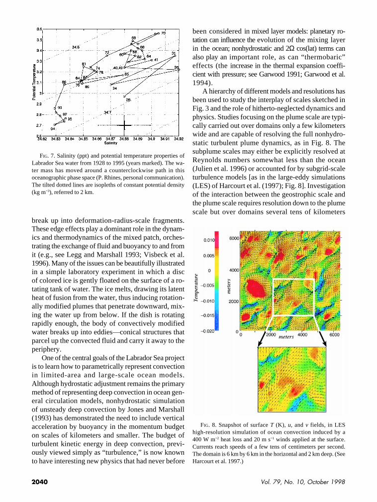
Observations of SST in hostile re-gions like the wintertime Labrador Seaare very sparse and are difficult to inter-pret because of the large (~6°C) annualcycle of SST. At about 100-m depth,however, the annual cycle is down to~1.5°C and decadal variability stands out(e.g., Levitus et al. 1994; Reverdin et al.1997). At 1000 m the annual cycle is0.2°C, decadal variability is muted, and10–100-yr variations dominate. Thegreat volume of LSW makes it a usefulstable reservoir for climate analysis.Over the past 100 yr, LSW has moved ina great counterclockwise loop in the po-tential-temperature/salinity diagram(Fig. 7). In the past decade or so the sys-tem has returned to a high 70-yr extremeNAO index, wonderfully deep convec-tion (to a depth of 2200 m in 1992), anda Labrador Sea resembling that in thefirst few decades of the century. Mean-while, as suggested by the seesaw be-tween the Greenland high and Icelandiclow, convection on the other side ofGreenland, in the Greenland Sea, hasbeen weak since the early 1980s.

c. Theory and modelingLaboratory and numerical studies of

oceanic convection have been central tothe planning of the field experiment and, particularlywhen used in concert with and scaled for comparisonwith the observations, have led to advances in ourunderstanding of the general problem of convectionin a rotating stratified fluid. Marshall and Schott(1998) review the key ideas and contributions in thecontext of the observations, models, and theory.

Two aspects make ocean convection interestingfrom a fundamental point of view. First, the timescalesof the convective process in the ocean are sufficientlylong that it may be modified by the earth’s rotation.Second, the convective and geostrophic scales are notvery disparate in the ocean and so the water masstransformation process involves a fascinating inter-play between convection and baroclinic instability(the interaction between phases II and III in Fig. 6).

This lack of a scale separation in the ocean should becontrasted with the atmosphere (e.g., see Fig. 2) wherethe convective scale (the “rolls” clearly evident in IRimage) have a much smaller scale than that of the syn-optic system in which they are embedded. This dif-ference in the parameter range of atmospheric andoceanographic convection can be usefully expressedin terms of the size of a “natural Rossby number” thatis small in the ocean but large in the atmosphere (seeJones and Marshall 1993; Maxworthy and Narimousa1994). Moreover, in the ocean large horizontal buoy-ancy gradients on the edge of the convection patchsupport strong horizontal currents in thermal-windbalance with them—the “rim current” (see Fig. 3). Ifthe patch has a lateral scale greater than the radius ofdeformation, then instability theory tells us that it must

FIG. 6. A schematic diagram of the three phases of open-ocean deep convec-tion: (I) preconditioning, (II) deep convection, and (III) lateral exchange andspreading. Buoyancy flux through the sea surface is represented by curly arrowsand the underlying stratification/outcrops by continuous lines. A boundary cur-rent runs around the periphery. Fluid overturned and mixed by convection isshaded. (From Marshall and Schott 1998.)

2040 Vol. 79, No. 10, October 1998

break up into deformation-radius-scale fragments.These edge effects play a dominant role in the dynam-ics and thermodynamics of the mixed patch, orches-trating the exchange of fluid and buoyancy to and fromit (e.g., see Legg and Marshall 1993; Visbeck et al.1996). Many of the issues can be beautifully illustratedin a simple laboratory experiment in which a discof colored ice is gently floated on the surface of a ro-tating tank of water. The ice melts, drawing its latentheat of fusion from the water, thus inducing rotation-ally modified plumes that penetrate downward, mix-ing the water up from below. If the dish is rotatingrapidly enough, the body of convectively modifiedwater breaks up into eddies—conical structures thatparcel up the convected fluid and carry it away to theperiphery.

One of the central goals of the Labrador Sea projectis to learn how to parametrically represent convectionin limited-area and large-scale ocean models.Although hydrostatic adjustment remains the primarymethod of representing deep convection in ocean gen-eral circulation models, nonhydrostatic simulationof unsteady deep convection by Jones and Marshall(1993) has demonstrated the need to include verticalacceleration by buoyancy in the momentum budgeton scales of kilometers and smaller. The budget ofturbulent kinetic energy in deep convection, previ-ously viewed simply as “turbulence,” is now knownto have interesting new physics that had never before

been considered in mixed layer models: planetary ro-tation can influence the evolution of the mixing layerin the ocean; nonhydrostatic and 2Ω cos(lat) terms canalso play an important role, as can “thermobaric”effects (the increase in the thermal expansion coeffi-cient with pressure; see Garwood 1991; Garwood et al.1994).

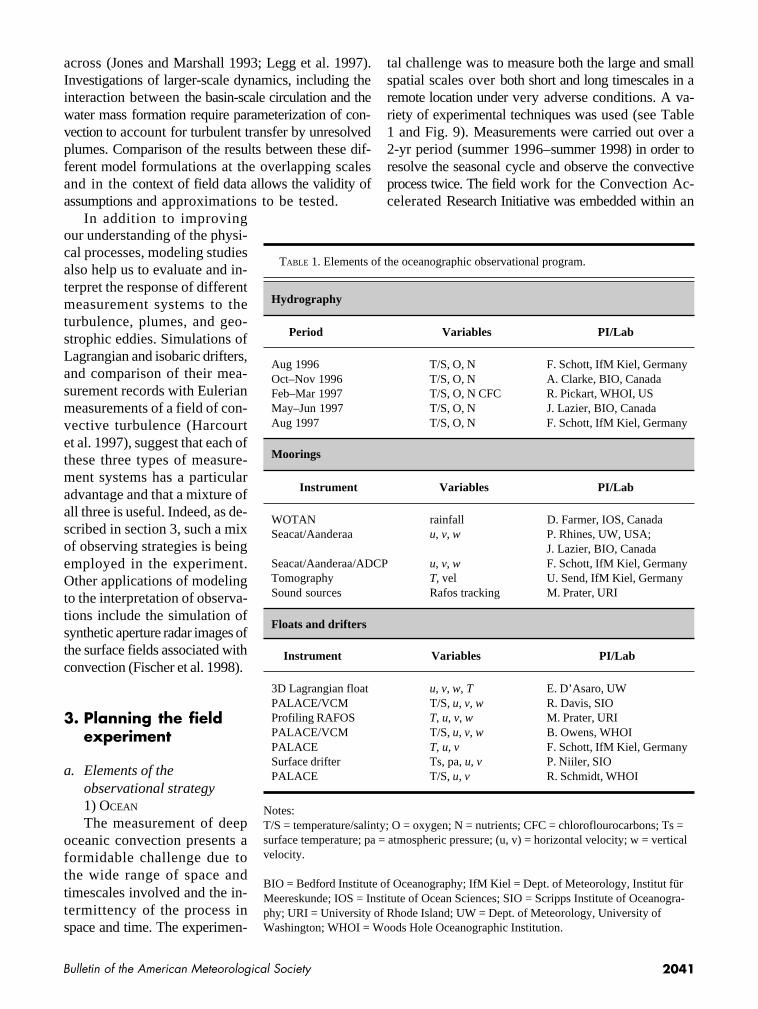
A hierarchy of different models and resolutions hasbeen used to study the interplay of scales sketched inFig. 3 and the role of hitherto-neglected dynamics andphysics. Studies focusing on the plume scale are typi-cally carried out over domains only a few kilometerswide and are capable of resolving the full nonhydro-static turbulent plume dynamics, as in Fig. 8. Thesubplume scales may either be explicitly resolved atReynolds numbers somewhat less than the ocean(Julien et al. 1996) or accounted for by subgrid-scaleturbulence models [as in the large-eddy simulations(LES) of Harcourt et al. (1997); Fig. 8]. Investigationof the interaction between the geostrophic scale andthe plume scale requires resolution down to the plumescale but over domains several tens of kilometers

FIG. 7. Salinity (ppt) and potential temperature properties ofLabrador Sea water from 1928 to 1995 (years marked). The wa-ter mass has moved around a counterclockwise path in thisoceanographic phase space (P. Rhines, personal communication).The tilted dotted lines are isopleths of constant potential density(kg m−3), referred to 2 km.

FIG. 8. Snapshot of surface T (K), u, and v fields, in LEShigh-resolution simulation of ocean convection induced by a400 W m−2 heat loss and 20 m s−1 winds applied at the surface.Currents reach speeds of a few tens of centimeters per second.The domain is 6 km by 6 km in the horizontal and 2 km deep. (SeeHarcourt et al. 1997.)


across (Jones and Marshall 1993; Legg et al. 1997).Investigations of larger-scale dynamics, including theinteraction between the basin-scale circulation and thewater mass formation require parameterization of con-vection to account for turbulent transfer by unresolvedplumes. Comparison of the results between these dif-ferent model formulations at the overlapping scalesand in the context of field data allows the validity ofassumptions and approximations to be tested.

In addition to improvingour understanding of the physi-cal processes, modeling studiesalso help us to evaluate and in-terpret the response of differentmeasurement systems to theturbulence, plumes, and geo-strophic eddies. Simulations ofLagrangian and isobaric drifters,and comparison of their mea-surement records with Eulerianmeasurements of a field of con-vective turbulence (Harcourtet al. 1997), suggest that each ofthese three types of measure-ment systems has a particularadvantage and that a mixture ofall three is useful. Indeed, as de-scribed in section 3, such a mixof observing strategies is beingemployed in the experiment.Other applications of modelingto the interpretation of observa-tions include the simulation ofsynthetic aperture radar images ofthe surface fields associated withconvection (Fischer et al. 1998).

3. Planning the fieldexperiment

a. Elements of theobservational strategy1) OCEAN

The measurement of deepoceanic convection presents aformidable challenge due tothe wide range of space andtimescales involved and the in-termittency of the process inspace and time. The experimen-

tal challenge was to measure both the large and smallspatial scales over both short and long timescales in aremote location under very adverse conditions. A va-riety of experimental techniques was used (see Table1 and Fig. 9). Measurements were carried out over a2-yr period (summer 1996–summer 1998) in order toresolve the seasonal cycle and observe the convectiveprocess twice. The field work for the Convection Ac-celerated Research Initiative was embedded within an

Aug 1996 T/S, O, N F. Schott, IfM Kiel, GermanyOct–Nov 1996 T/S, O, N A. Clarke, BIO, CanadaFeb–Mar 1997 T/S, O, N CFC R. Pickart, WHOI, USMay–Jun 1997 T/S, O, N J. Lazier, BIO, CanadaAug 1997 T/S, O, N F. Schott, IfM Kiel, Germany

TABLE 1. Elements of the oceanographic observational program.

Notes:T/S = temperature/salinty; O = oxygen; N = nutrients; CFC = chloroflourocarbons; Ts =surface temperature; pa = atmospheric pressure; (u, v) = horizontal velocity; w = verticalvelocity.

BIO = Bedford Institute of Oceanography; IfM Kiel = Dept. of Meteorology, Institut fürMeereskunde; IOS = Institute of Ocean Sciences; SIO = Scripps Institute of Oceanogra-phy; URI = University of Rhode Island; UW = Dept. of Meteorology, University ofWashington; WHOI = Woods Hole Oceanographic Institution.

Hydrography

Period Variables PI/Lab

3D Lagrangian float u, v, w, T E. D’Asaro, UWPALACE/VCM T/S, u, v, w R. Davis, SIOProfiling RAFOS T, u, v, w M. Prater, URIPALACE/VCM T/S, u, v, w B. Owens, WHOIPALACE T, u, v F. Schott, IfM Kiel, GermanySurface drifter Ts, pa, u, v P. Niiler, SIOPALACE T/S, u, v R. Schmidt, WHOI

Moorings

WOTAN rainfall D. Farmer, IOS, CanadaSeacat/Aanderaa u, v, w P. Rhines, UW, USA;

J. Lazier, BIO, CanadaSeacat/Aanderaa/ADCP u, v, w F. Schott, IfM Kiel, GermanyTomography T, vel U. Send, IfM Kiel, GermanySound sources Rafos tracking M. Prater, URI

Instrument Variables PI/Lab

Floats and drifters

Instrument Variables PI/Lab

2042 Vol. 79, No. 10, October 1998

array of autonomous floats deployed as part of theWOCE Atlantic Circulation and Climate Experiment,which mapped out the large-scale circulation.

The three-dimensional structure of the LabradorSea gyre was revealed by numerous hydrographic sec-tions across the basin during four cruises in 1996–97.These three-dimensional data were complemented byacoustic tomography, measuring average propertiesbetween several moored acoustic transceivers (seeSend et al. 1995). In addition, the WOCE AR-7 hy-drographic section (see Fig. 9) was heavily instru-mented with moorings measuring velocity, salinity,and temperature throughout the water column at hightemporal resolution.

Finally, freely drifting surfacedrifters and subsurface floats ofvarious designs provided an eco-nomical way to measure a widerange of space and timescales. Alarge number (> 150) of such de-vices have been deployed (seeFig. 9). All measure horizontal ve-locity and temperature at their lo-cation; some measured verticalvelocity, a clear signature of con-vection. Others periodically pro-filed the T/S structure of the watercolumn, moving up to the surfaceand relaying data back to base be-fore dropping down to their refer-ence level again. A broad range ofspatial scales was sampled by de-ploying the instruments in bothsmall- and gyre-scale arrays.

2) ATMOSPHERE

The fluxes of heat, moisture,and radiation across the air–sea in-terface are the primary agents re-sponsible for the densification ofthe surface waters that triggersconvection. The objective of themeteorological component of theexperiment was to document thesurface fluxes and to understandthe mechanisms responsible forthem. Our measurements benefitedfrom the larger-scale context pro-vided by the FASTEX experiment(Joly et al. 1997).

Historically, there have been nodirect measurements of the fluxes of heat, momentum,and moisture across the air–sea interface in the Labra-dor Sea—only bulk estimates. As a result, the confi-dence that one can have in model-derived estimatesof these fluxes is reduced. It was therefore decided tocollect in situ data during a winter oceanographiccruise of the R/V Knorr to test flux estimates of nu-merical models and observe the detailed evolution ofthe atmospheric boundary layer. Measurements of thefluxes of incoming solar radiation, momentum, sen-sible and latent heat, water vapor, and precipitationwere carried out by a consortium of groups. To im-prove our understanding of the structure and evolu-tion of weather systems over the region and to

FIG. 9. Map showing elements of the oceanographic field program. The hydrographicstations occupied by the Knorr during February and March 1997 are indicated, as arethe floats deployed from Knorr (colored symbols; see key). Also shown are the posi-tion of the moorings (open circles), the Central Float Deployment (CFD) region andthe tomographic array. Many other floats were deployed in cruises both before and afterthat of the Knorr. The Ks indicate the position of Kiel moorings, the Bs are boundarycurrent moorings, Ws are inverted echo sounders, and SSs are RAFOS sound sources.Investigators involved in the field program are indicated in Table 1.


facilitate model initialization and verification efforts,radiosonde launches were also made from the Knorr.Table 2 outlines the wide variety of activities associ-ated with the science program on the Knorr. In tan-dem with the ship program, several aircraft missionswere flown to document the synoptic-scale environ-ment over the region and to make measurements ofthe mesoscale structures that modulate air–sea inter-action in the region.

There was also a remote sensing component to theexperiment. Images were collected at prespecifiedtimes and locations from the Canadian Radar Satel-lite Synthetic Aperture Radar (SAR) and data werecollected on an ad hoc basis from the European Sat-ellite Agency European Remote-sensing Satellite-2(ERS-2) SAR, scatterometer, and radar altimeter. Twowell-equipped aircraft (a CV-580 from the CanadaCentre for Remote Sensing and a P3 from NASA/Goddard Space Flight Center) flew over the ship onseparate 4-day missions collecting sea surface andmean meteorological profile data using a wide vari-ety of instruments.

b. Anticipating where convection will happenDuring the planning stages of the convection ex-

periment we began to recognize that decadal climatevariability reviewed in section 2b and the vagaries ofthe NAO might interfere with our goal to observe deepconvection in the Labrador Sea. The winter of 1993had resulted in an extremely active convection seasonpenetrating down to more than 2200-m depth, but insubsequent winters convection never reached thosedepths again and in fact the winter of 1995–96 resultedin convection that was probably no deeper than1000 m.

With the drop in the NAO index during the win-ter of 1995–96 we feared a second weak winter. It wasclear that we had to make sure that the instrumentsdesigned to observe deep mixing were deployed in anoptimum way. Luckily we were in a position to de-ploy deep mixed layer floats during the early part ofthe Knorr winter survey, just a few weeks prior to theexpected deepest mixing. But where, precisely, shouldwe put them?

Starting in October 1996 we began predicting sev-eral convection scenarios using both a high-resolutionnumerical model (Marshall et al. 1997) and real-timedata coming in from some 30 profiling AutonomousLagrangian Circulation Explorer (PALACE) floats,whose position in February 1997 is indicated inFig. 10. The temperature and salinity profiles provided

by these floats were used to compute the stratificationand obtain estimates of how much buoyancy was heldin the water column. This buoyancy content was com-pared to the expected buoyancy loss between the timeof “forecasting” and the end of the winter season inlate March, enabling us to predict how deep convec-tion might reach assuming it to be a one-dimensional(1D) process. The expected depth to which the mixedlayer would reach in a moderate winter (defined as onein which there was only 80% of a typical wintertimebuoyancy loss) assuming nonpenetrative deepening,is indicated in Fig. 10. As reviewed in section 4a, earlyin the winter heat losses were relatively weak raisingsome concern, but our predictions suggested that wewould still have a reasonable chance of observingmixing down to a depth of 800–1000 m. Nevertheless,it was decided to withhold half of the floats to be ableto spread the risk over two convection seasons; theremainder were deployed in the second phase of thefield work, in January 1998. By early January 1997 itbecame clear that an interesting pattern of stratifica-tion was revealed by the PALACE floats (see Fig. 10):the sea was strongly stratified to the north and to thesouth, but a band of weak stratification existed inthe middle, some 3° in width centered at 56°N.Combining this information with the climatologicaldistribution of oceanic heat loss that shows a maxi-mum just eastward of the Labrador coast (see Fig. 4)we identified an area of weakest stratification andexpected maximum heat loss (the “yellow” region inFig. 10). This “prediction” also found support fromthe high-resolution numerical model of the LabradorSea developed by C. Herbaut and J. Marshall (1998,personal communication) (see Fig. 11).

Based on the above considerations, a few daysbefore the Knorr left Halifax, Nova Scotia, Canada,it was decided to deploy the floats in a central floatdeployment (CFD) area [the box marked in Fig. 9,roughly coinciding with the position of the convec-tion patch observed by Clarke and Gascard (1983);also see the shaded patch in Fig. 1]. During early Feb-ruary the float array was deployed. From October untilthe middle of February our predictions of mixed layerdepth, based on the assumption of a moderate winter,remained unchanged at 800–1000 m. However, to ourgreat delight and as described in section 4b, by the endof the Knorr cruise (12 March) the mixed layer hadreached a maximum depth of 1500 m in one spot50 km southward of our best-guess estimate. The cy-clonic circulation pattern over the North Atlantic hadintensified during February, resulting in heat losses

2044 Vol. 79, No. 10, October 1998

Rawinsonde, 6–12 day U,D,Td, Ta Guest/NPGS Guest/NPGS, IfM Kiel

Solar pyranometer SW + LW incoming Guest/NPGS Guest/NPGS, IfM Kiel

Laser ceilometer CeilingHt, CloudHt White/ETL Guest/NPGS

3 GHz precipitation radar VertVel Liq. H2O Costa/ETL Dobson/BIO

Ship rain gauge P Uhlig/Kiel Uhlig/Kiel

Disdrometer P, P′ Grossklaus/Kiel Uhlig/Kiel

Disdrometer P, P′ Hare/ETL Dobson/BIO

IR cloud temp Tcloudbot

Uhlig/Kiel Uhlig/Kiel

IR sea temp Ta Guest/NPGS Guest/NPGS

“Sea snake” Ta Hare/ETL Dobson/BIO

Intake temp Ta IMET/WHOI Pickart/WHOI

Pl. res. therm. Ta Hare/ETL Dobson/BIO

Thermistor Ta IMET/WHOI Pickart/WHOI

Fast thermometer Ta, Ta′ Bumke/Kiel Uhlig/Kiel

Thermistor Ta, Ta′ Anderson/BIO Anderson/BIO

Thermistor Ta, Ta′ Anderson/BIO Anderson/BIO

Hygrometer RH IMET/WHOI Pickart/WHOI

Dewflinger e′ Aktaturk/UW Anderson/BIO

Hygrometer h′, CO2′ Hare/ETL Anderson/BIO

Wind monitor U, D, u′, d′ Anderson/BIO Anderson/BIO

Gill sonic anem. U, D, Ta, u′, v′, w′, ta′ Anderson/BIO Anderson/BIO

Anemometer U, D, Ta, u′, v′, w′, ta′ Bumke/Kiel Bumke/Kiel

Motion package ai, Tilt

iUhlig/Kiel Uhlig/Kiel

Gyrocom-pass Ship’s course IMET/WHOI Pickart/WHOI

Gyrocom-pass Ship’s course Hare/ETL Dobson/BIO

Doppler log Ship’s speed IMET/WHOI Pickart/WHOI

GPS Ship’s position IMET/WHOI Pickart /WHOI

Marine radar Wave field Trizna/NRL Dobson/BIO

Wave height gauge Wave height Dobson/BIO Dobson/BIO

Directional buoy Wave dirn. spec Dobson/BIO Dobson/BIO

TABLE 2. Meteorological and air–sea flux measurements on R/V Knorr.

Instrument Variable(s) Owner/Lab PI

Caps = Mean quantities; primes = fluctuations about the means; U, u = wind speed; D, d = wind direction; v, w = wind componentscrosswinds, vertical; Ta = air temperature; Ts = sea surface temperature; h = absolute humidity; CO

2 = CO

2 content; a =

acceleration; P = precipitation; e = water vapor; IMET = improved meteorological measurement system; Pl. res. therm. = platinumresistance thermometer.ETL = Environmental Technology Laboratory, NOAA; NPGS = Naval Postgraduate School.


greatly exceeding climatological values (see section4a), which induced deeper-than-expected convection.

4. Preliminary results from the 1996–97experiment

a. The atmospheric forcing during the winter of19971) SYNOPTIC CONDITIONS DURING WINTER 1997The winter of 1997 provided an excellent oppor-

tunity to document the variability in the air–sea inter-action that exists within a given winter season. Figure12 shows the average mean sea level pressure, 10-mwind, and total heat flux fields for January 1997(Fig. 12a) and February 1997 (Fig. 12b) as determinedfrom the NCEP–NCAR Reanalysis project. A com-parison between the two months and the winterclimatology (Fig. 5) shows that a dramatictransition occurred in the flow regimeover the North Atlantic and that this re-sulted in a significant change in the mag-nitude of the surface cooling in theLabrador Sea region. January 1997 wasa month in which the circulation over theNorth Atlantic was significantly differ-ent from the winter climatology; thepresence of a blocking high overEurope and anomalously strong highpressure over Greenland resulted in asignificant westward shift in the centerof cyclonic activity. It is interesting tonote that even with this weakening of thecyclonic flow over the North Atlantic,the mean total heat loss in the center ofthe Labrador Sea was, at 260 W m−2,larger than the climatological wintermean. In contrast, February 1997 was amonth in which the circulation patternover the North Atlantic was significantlystronger than average. As one might ex-pect in such a flow configuration, themean heat loss in the center of the La-brador Sea, some 420 W m−2, was sig-nificantly above the climatologicalwinter mean (see Table 3). These ex-tremely high oceanic heat losses contrib-uted to making what might otherwisehave been a lackluster winter, from theperspective of forcing deep convection,into a “good” winter.

2) VARIABILITY IN HEAT AND MOISTURE FLUXES

DURING THE WINTER OF 1997Although a period of one month is a convenient

period of time over which to average, the influence andphasing of individual events tends to be lost by suchaveraging. Another and perhaps more illuminatingview of the variability of air–sea interaction in the La-brador Sea during the winter of 1997 is depicted inFig. 13. This figure shows the 6-hourly values of meansea level pressure at a location in the center of the cli-matological Icelandic Low (62°N, 30°W; Fig. 13a) andtotal heat flux at the Bravo site (56°N, 51°W; Fig. 13b)as determined from the NCEP–NCAR Reanalysis. Itis clear that the North Atlantic flow regime in Decem-ber 1996 and early January 1997 was significantlydifferent from that in the latter part of the winter. Thegenerally high sea level pressure and weak cyclonicactivity in the early part of the winter can be classi-

FIG. 10. Position of PALACE floats (black discs; courtesy of R. Davis) at thebeginning of February 1997. Based on the measured buoyancy content in the watercolumn at these positions, climatological estimates of the buoyancy loss from thesurface, estimates of the expected maximum depth of the mixed layer are indi-cated in meters (courtesy of M. Visbeck) assuming a moderate winter (defined as80% of the climatology), and a 1D, nonpenetrative process. The region of weak-est stratification is marked. Its overlap with the region of maximum buoyancy lossto the atmosphere led to our prediction of the position of deepest mixed layer depth(marked yellow). This, together with the numerical model results shown in Fig. 11,guided our choice of position of the CFD area.

2046 Vol. 79, No. 10, October 1998

fied, according to Vautard (1990), as being associatedwith either a “blocking” or “Greenland anticyclone”regime, while the low sea level pressure and strongcyclonic activity during the latter part of the winter

belongs to a more “zonal” flow regime. The first twoweeks of January were unusual in that the pressure nearIceland underwent a monotonic decrease. This changein flow regime had a dramatic impact on the surfacecooling that was taking place in the Labrador Sea.From December 1996 to 15 January 1997 the averagetotal heat flux at the Bravo site was only 150 W m−2.Indeed, the lowest heat fluxes occurred during the firsttwo weeks of January. Over the flowing six-week pe-riod ending on 28 February 1997, however, it was inexcess of 420 W m−2 with peak fluxes greater than1000 W m−2.1 There is significant high-frequencyvariability in the magnitude of the total heat flux, asignature of the passage of North Atlantic cyclones.This can be seen from the high degree of anticorrela-tion that exists between the two time series (seeFig. 13). Furthermore, the data explain why the sur-face cooling during January was above the climato-logical mean even though the monthly mean sea levelpressure field indicated a weaker than average cyclonicflow over the North Atlantic. The more vigorous cy-clonic circulation that developed after the middle ofthe month and the concomitant elevated heat fluxes ledto a large monthly mean heat flux for January.

With a few exceptions, the time series of precipi-tation is similar to that of the total heat flux. The high-est precipitation rates, in excess of 2 mm h−1, occurredin late January and February. A careful examinationof the phasing of the precipitation and total heat fluxmaxima in the Labrador Sea region indicates that theformer typically leads the latter by approximately oneday. This is a consequence of the structure of a typi-cal extratropical cyclone, such as the one shown inFig. 2, which results in a separation of the region ofhigh precipitation from that of high heat flux.

Table 3 presents monthly mean values of the totalheat flux from NCEP–NCAR, precipitation rate, andnet radiative flux at the historic location of the OceanWeather Station Bravo (56°N, 51°W) for the monthsof December 1996, and January, February, and March1997. December 1996 was a month in which thefluxes of heat and momentum were anomalously low,when compared to the 30-yr mean for the month ofDecember. In contrast, January and February 1997were months in which these fluxes exceeded the 30-yrmeans. When considered as a whole, the winter of

FIG. 11. Simulation of water mass transformation in a high-resolution model of the Labrador Sea developed by C. Herbautand J. Marshall (1998, personal communication): (a) hydrographicsection of temperature across the model’s AR-7 section, (b) cur-rents at a depth of 100 m showing the boundary current and ed-dies, and (c) mixed layer depth in March 1992 obtained by drivingthe model with NCEP winds and fluxes starting in summer 1991.The position of the region of deepest mixed layer is roughly co-incident with that indicated in Fig. 10.

1It is important to note that there is a clear discrepancy betweenanalyzed fluxes and the bulk estimates from the Knorr; com-pare Fig. 14 with Fig. 13, for example. Are they real or the resultof differences in sampling or of reporting?


1997 was one in which thefluxes of heat, moisture, and netradiation exceeded the 30-yrmeans by approximately onestandard deviation and so washighly conducive to convectiveactivity in the Labrador Searegion.

3) AIRCRAFT AND REMOTE

SENSING MISSIONS

The meteorological aircraftstudies consisted of three mis-sions over the Labrador Sea.Flight planning took into ac-count the position of the Knorrand meteorological conditionsreported from the ship, and onone occasion sampling tookplace in the vicinity of the ship.The flights were completed dur-ing February 1997 with researchaircraft from the 53d WeatherReconnaissance Squadron ofthe U. S. Air Force. The C-130aircraft used were equipped withdropsonde systems and wereable to record state parametersat flight level. To assist in flightplanning, as described inRenfrew et al. (1998), the NavalResearch Laboratory ran a spe-cial version of their CoupledOcean–Atmosphere MesoscalePrediction System (COAMPS) (see Hodur 1997) re-gional atmospheric forecast model over a domain thatincluded the Labrador Sea twice daily out to 36 h. Themodel data, including all important surface fields suchas the heat, radiative, and moisture fluxes, were madeavailable in real time to scientists in the field, greatlyhelping the planning process. These data were alsoused to generate daily synoptic weather summaries andforecasts for use by the Knorr in scheduling opera-tional and scientific ship activities.

Two remote sensing aircraft programs were car-ried out over the Knorr during the experiment. On22–24 February a Convair 580 from the Canada Cen-tre for Remote Sensing equipped with a C-band syn-thetic aperture radar flew a series of four missions,imaging the ship and the waters around her to deter-mine the effects of polarization on the ability of the

instrument to image the sea surface. On 3–9 March aP-3 aircraft from NASA flew four ocean wave imag-ing and passive microwave missions over the ship.Both missions carried out intensive surface meteoro-logical and wave measurements in concert with theshipboard measurement program. In addition, ERS-2SAR images of the ocean surface were obtained andattempts made to identify the surface signature of deepocean convection by using hydrodynamic models ofconvection and a sensor model for SAR (see Fischeret al. 1998). Identification of a convective surface sig-nature could allow unique information about the spa-tial characteristics of the convective process to bedetermined such as the extent of convecting region,the size of individual convective plumes and eddies,the ratio of converging to diverging area, and the sur-face current strain. Initial results, though speculative

FIG. 12. Average mean sea level pressure (contour, mb), 10-m wind (vector, m s−1) andtotal heat flux (shaded, W m−2) fields from the NCEP–NCAR Reanalysis for (a) the monthof January 1997 and (b) the month of February 1997.

2048 Vol. 79, No. 10, October 1998

in nature, showed several scenes that had an appear-ance that mimicked model results.

4) IN SITU MEASUREMENTS FROM THE KNORR

The R/V Knorr was in the Labrador Sea properfrom 7 February to 12 March 1997. During that pe-riod the atmospheric conditions were surprisingly con-sistent and in the “zonal regime”. Most of thelow-pressure systems that approached from the southand west tracked to the south of the ship, and for vir-tually the entire cruise the wind direction was west-erly to northerly. Upper-air winds were generally fromthe west. We were in a “cold air outbreak” regime (seeFigs. 2 and 12b).

At this early stage in the analysis what is reallyavailable to us, besides real-time uncalibrated esti-mates of the fluxes from our on-line logging systems,are bulk flux estimates and the evidence of our senses.They tell us that the entire period was dominated by aflow of cold dry air from the northwest, intense trans-fers of heat and water vapor to the atmosphere, ever-present precipitation in the form of snow squalls, andrapid deepening of the oceanic mixed layer. Table 4indicates the ranges and types of meteorological con-ditions encountered during the cruise.

Figure 14 is a plot of preliminary time series of air-sea fluxes as deduced from heat and momentum trans-fers encountered during the cruise of the Knorr. (Thebulk meteorological parameters on which they arebased have not been fully corrected, although the

Total heat flux (W m−2) 117 258 422 227 271(30-yr mean and (189 ± 64) (223 ± 91) (247 ± 98) (198 ± 88) (223 ± 59)standard deviation)

Precipitation rate (mm h−1) 0.114 0.247 0.175 0.192 0.182(30-yr mean and (0.167 ± 0.043) (0.162 ± 0.050) (0.137 ± 0.046) (0.114 ± 0.039) (0.147 ± 0.028)standard deviation)

Net radiative flux (W m−2) 53.2 50.8 44.8 −20 32(30-yr mean and (57 ± 7) (55 ± 10) (25 + 10) (−25 ± 7) (28 ± 5)standard deviation)

TABLE 3. Fluxes and precipitation from the NCEP–NCAR Reanalysis.

Dec Jan Feb Mar Winter of1996 1997 1997 1997 1997

Mean values of the total heat flux (W m−2), precipitation rate (mm hr−1) and net radiative flux (W m−2) at 56°N,51°W for the monthsof December 1996 and Jan–Mar 1997 as diagnosed from the NCEP–NCAR Reanalysis. Also shown are the means for the winterof 1997 (1 Dec–31 Mar 1996 inclusive). The 30-yr means for the various time periods as well as the standard deviation from themeans are also shown.

FIG. 13. (a) Six-hourly valves of mean sea level pressure (mb)at 62°N, 30°W and (b) total heat flux (W m−2) at 56°N, 51°W forthe period 1 December 1996–1 April 1997 as determined fromthe NCEP–NCAR Reanalysis.


winds have been transformed from rela-tive to the ship into absolute.) We havemade no attempt to separate the data intoperiods when the ship was still or mov-ing, so the time series is a mix of time andspace. The large heat fluxes to the atmo-sphere are a reflection of the environmentthe ship was working in, but note thatthey are somewhat smaller than those im-plied by the models (see Fig. 13). Theyare largest in magnitude at times whenthe ship approached the ice pack on theLabrador coast.

It is interesting to use the averageof the total heat flux to compute thecooling effect of the fluxes themselves.Assuming that a layer of ocean 1000 mdeep was cooled over the course of theKnorr’s stay in the Labrador Sea, theaverage flux of 360 W m−2 would havecooled that water by about 0.24°C. Thisis a representative calculation only, be-ing a combination of the fluxes at differ-ent locations in the Labrador Sea atdifferent times. Nevertheless, the heat loss as mea-sured by the CTD was very close to what would beexpected based on the ship measurements.

Estimates of mean evaporation E and precipitationP for the period are incomplete at time of writingand hence inaccurate. Based on the bulk latent heatflux from Table 4, E is about 5 mm day−1; basedon visual estimates of snow accumulation rates ondeck, P is 5–15 mm day−1, in both cases of liquidwater. We intend to improve both, using eddy corre-lation latent heat fluxes for E and disdrometer mea-surements for P.

Heat was lost over the entire sea, but by differentmechanisms in different parts of the area. Near thewestern boundary, the precipitation was at a minimumbut the measured upward fluxes of heat and water va-por were the largest. The snow squalls occupied moreof the total surface area as we progressed eastward, sothat from one-third of the way from the west to the eastside it snowed more or less continuously. Whereas thenet moisture transfer was upward on the western side,it was downward over most of the remainder of thearea. This downward flux of moisture as precipitationwas necessarily accompanied by an upward transferof heat, since the water that received the snow had togive up the latent heat of fusion as well as some sen-sible heat. Thus there was upward transfer of heat over

the entire sea, but the flux of buoyancy was upwardon the western side and downward to the east. Usinga bulk surface heat flux method (Smith 1988), the av-erage sensible heat flux during the time the ship wasin the Labrador Sea proper was about 160 W m−2. Theaverage latent heat flux was about 150 W m−2.

The spatial distribution of observed heat and mois-ture transfer suggests that at least during cold air out-breaks (northwesterly winds), the Labrador Sea forcesa strong coupled response in the atmosphere and thatthe air–sea transfers ensure that the entire atmosphere–ocean system can be treated (and modeled) as a singlecoupled process. However, when the wind is from thesouth (a rare occurrence over the duration of the cruise)there is a ready supply of warm advective moisture forprecipitation.

In addition to surface atmospheric measurements,many upper-air rawinsonde profiles were performedfrom the Knorr, the only rawinsonde measurementsever undertaken in the central part of the Labrador Sea.The upper-air profiles demonstrated that deep convec-tion existed in the atmosphere as well as in the ocean.Figure 15 shows three examples: the deepest atmo-sphere boundary layer (ABL) observed during thecruise (0500 UTC 9 February), a more typical bound-ary layer in the same location a few hours later(1400 UTC 9 February), and a relatively shallow ABL

FIG. 14. Time series of surface fluxes and wind stress as deduced from con-tinuous shipboard measurements on the Knorr as it moved around the LabradorSea taking hydrographic sections and deploying floats (courtesy of F. Dobson andP. Guest). Investigators involved in the meteorological measurements taken fromthe Knorr are indicated in Table 2.

2050 Vol. 79, No. 10, October 1998

just downwind of the ice edge (22 February). In gen-eral, the ABL tended to be shallowest just off the up-wind ice edge (as in the 22 February case) and itdeepened rapidly offshore. However, considerabletemporal variability (e.g., see the two 9 February pro-files plotted in Fig. 15) prevented a detailed assess-ment of spatial variations in ABL characteristics fromthe ship data alone. One of the significant effects ofthe deep ABLs was that the temperatures and humidi-ties required considerable time to adjust to the seasurface conditions due to the large quantity of air thathad to be modified. Evidently, in cold air outbreaksover the Labrador Sea, the temperatures and humidi-ties remain low and large turbulent sensible and la-tent heat fluxes extend all the way across the LabradorSea.

b. The response of the ocean1) WINTER CRUISE: 7 FEB–12

MARCH 1997(i) HydrographyThe planned cruise track was de-

signed to cover a broad area of the La-brador basin, with emphasis on thewestern sector (see Fig. 9). After repeat-ing the along-basin section of the fallcruise (October–November 1996) itwas evident that the developing regionof deepest convection was of limitedlateral extent. Cross-basin sections werethus placed more closely together, and“dog-legs” devised in order to achievea broad coverage (Fig. 9). We ensuredthat detailed boundary crossings weremade on both sides of the basin (on theLabrador side these were limited by theice pack) so that the role of the warm–salty Irminger water on both the con-vection and restratification processcould be addressed. The central cross-basin section, where the deepest mixedlayers were observed, was repeated asecond time in order to shed light on therelative influence of vertical versushorizontal advection. Finally, we per-formed two detailed fine resolutionCTD surveys, the second of which cap-tured the deepest convection of the ex-periment (1500 m).

There were numerous surprises thatwill require further analysis using thecombined resources of the convection

experiment. The rapidity at which the oceanic mixedlayer deepened during the cruise was impressive. Oneof the CTD stations on the central cross-basin sectionwas repeated three times during the 5-week period. Asimple 1D mixed layer model (Pickart and Smethie1998) required a sustained forcing of 1000 W m−2 toproduce the observed mixed layer depths of the sec-ond and third occupations. This buoyancy loss is sig-nificantly greater than that observed, suggesting thatthe mixed fluid must have been advected from else-where to the point at which it was observed. Anothersurprise was how close convection occurred to thewestern boundary. In fact, the deepest observed mixedlayers were near the 3100 m isobath, close to the coreof the deep western boundary current with importantramifications for the spreading process. One view is

Air pressure (mb) 973.1 1017.3 994.9 10.3

Wind speed (m s−1) 0.4 24.7 11.7 3.9

Wind direction 291

Air temp (°C) −17.11 4.15 −7.84 3.80

Sea sfce temp (°C) −1.47 5.72 2.89 5.72

Relative humidity (%) 42.0 95.8 68.7 9.0

Wind stress (Pa) 0.0009 1.274 0.274 0.180

Sens heat flux −15.6 374.2 163.5 79.9

Latent heat flux −1.8 305.1 147.1 54.8

Net SW rad flux −524.3 0.0 −33.1 61.7

Net LW rad flux 11.0 174.0 84.3 24.7

Net rad flux −422.1 165.7 51.1 62.9

Total heat flux −255.3 732.7 361.7 160.8

TABLE 4. Range of meteorological conditions encountered during Knorr cruise.

Min Max Mean Std dev

Notes:1. These statistics are based on 5-min averages of the 15-s samples of the Knorr’sIMET system (sensor height 23 m) and samples from the U.S. Naval PostgraduateSchool’s radiation measurement system. They cover only the period from 0000UTC on 8 Feb 1997 until 24 UTC on Mar 13, when the Knorr was actually in theexperimental area.2. All heat fluxes are in W m−2, and positive upward (out of the ocean).


that convection occurs in the center ofthe western cyclonic gyre (e.g.,Clarke and Gascard 1983), thenslowly spreads outward, predomi-nantly by the action of baroclinic in-stability (Legg and Marshall 1993;Visbeck et al. 1996). Instead our ob-servations suggest that some of theconvected water may directly pen-etrate the western boundary current,thereby providing a swift escape routeto southern latitudes. The increasedsurface salinity near the boundary, in-fluenced by the Irminger water, mayalso play a role in the deep mixed lay-ers observed there.

Throughout, the convection wasobserved to be accompanied by defor-mation-scale (~10 km) geostrophiceddies and baroclinic instability.Toward the end of the cruise, particu-larly during the repeat of the centralcross-basin section (see Fig. 9), wesurmise that measurements wereconducted during or shortly afteractive convection. The spatial vari-ability in the CTD casts was remark-able. Intrusions were prevalent, andoften the downcast trace would differsignificantly from that of the upcast.Our second CTD tow-yo survey cap-tured the capping-over of a convectivepatch, complete with numerous suchintrusions. Some of this rich structuremay be due to the proximity of con-vection to the boundary, where strongcontrasts exist between resident watermasses. Finally, we found that the re-gion of deep convection was ratherconfined laterally, as revealed by thedistribution of observed mixed layerdepth (Fig. 16). This map is aliasedin time with, for example, a ridge ofshallow mixed layer depth corre-sponding to the along-basin section,which was occupied early in thecruise. Eventually this map will be ad-justed for synopticity using all theavailable time series information. Therelative importance of atmosphericforcing versus oceanic precondition-

FIG. 16. Mixed layer depth deduced from the Knorr hydrography, an average overthe period 7 February–12 March 1997. The deepest convection is localized to thewest, where a mixed layer of depth 1100 m is observed (courtesy of R. Pickart).

FIG. 15. Potential temperature vs height from the 1997 Knorr Labrador Sea cruisebased on rawinsonde (weather balloon) profiles. Regions of near-constancy of po-tential temperature with height are indicative of convection in the atmospheric bound-ary layers. The potential temperature of 0500 UTC 9 February increases slightlybetween 1200 and 4500 m (following a “pseudo-adiabat”) due to latent heat releasewithin a cloud, but is indicative of a well-mixed layer of depth ~4 km forming theABL. The ABL depths on 1400 UTC 9 Feb and 2300 UTC 22 Feb are 1250 and 980 m,respectively (courtesy of P. Guest).

2052 Vol. 79, No. 10, October 1998

ing in setting the relatively confined scale of themixed patch needs to be addressed.

(ii) TracersThe chlorofluorocarbons (CFCs) CFC-11,

CFC-12, and CFC-113 were measured at 44 of thehydrographic stations and provide a vivid record of

convective activity. CFCs enter the ocean at the sur-face and become incorporated in LSW during the deepconvective process. In Fig. 17 the basin-scale distri-bution of CFCs is shown along the AR7 section (seeFig. 9 for position). The highest surface water CFCconcentrations, close to equilibrium with the atmo-sphere, were observed at the margins of the LabradorSea where convection was not occurring. In the cen-tral Labrador Sea, surface water concentrations werelower and well below equilibrium with the atmosphereas a result of deep convection transporting CFCsdownward faster than they entered the surface waterby gas exchange. LSW is readily identifiable in theCFC distribution as two distinct homogeneous layers,an upper layer extending from the surface to 500–1000-m depth and a deeper layer extending from thebase of the upper layer to a depth of about 2200 m.The upper layer is LSW that has just formed, deeperon the western side of the section. The deeper layerwas formed during a previous winter when convec-tion reached to ~2 km, probably in February andMarch 1992, as discussed in section 2b.

2) FLOATS

(i) Profiling floats (PALACE) andvertical current meters (VCM)

These floats periodically dive todepths near 1600 m collecting profilesof temperature and salinity. By adjust-ing buoyancy, the float then moves toa preprogrammed depth of either 1500or 600 m where it follows currents forperiods of 10 or 20 days. It then risesto the surface for 24 h during whichtime profile data is relayed to Argossatellites, which also locate the float.After this surface period, the onlytime when float position is known, theinstrument descends to collect anotherprofile and velocity observation.

Figure 18 shows as colored vec-tors the trajectories of 36 WOCEfloats deployed between November1996 and January 1997 and 8 similarNOAA floats deployed in 1994 and1995. These floats map out some ex-pected and unexpected aspects of thecirculation and should be comparedwith the schematic shown in Fig. 1.They show the Greenland Currentas a strong boundary current off the

FIG. 18. The trajectories PALACE floats in the Labrador Sea. Colored vectorsindicate submerged displacements over 10–20 days of floats drifting between 600and 1500 m deployed between 1994 and 1997. Black vectors indicate the submergeddisplacement of VCM floats deployed near 400 m as part of the Convection ARI.These are 4-day displacements (courtesy of R. Davis).

FIG. 17. Vertical distribution of CFC-11 (pmol kg−1) along-line AR7 of the Knorr winter Labrador Sea cruise. The dataare preliminary, based on shipboard calculations (courtesy ofW. Smethie).


Greenland coast; sustained flows up to 25 cm s−1 areobserved off the southwest coast. This flow generallyfollows the bathymetry across the northern LabradorSea, forming the intermediate depth portion of thesouthwestward flowing Labrador Current that even-tually makes its way past the Grand Banks of New-foundland. These boundary currents surround thecentral Labrador Sea, where organized flows are weakcompared to the substantial synoptic-scale variabil-ity. In most places there is no apparent pattern.

A signature of convection in the Labrador Sea isthe mixing of relatively fresh surface waters to in-creasing depth as surface fluxes extract buoyancyfrom the upper-water column. Figure 19 shows a timeseries of potential temperature and salinity profilesfrom a float deployed near 60.5°N, 57°W that movedsoutheastward roughly paralleling isobaths (it ismarked purple in Fig. 18). As time progresses, coolupper-layer temperatures erode the thermocline tem-perature maximum until it disappears; simulta-neously, freshwater is mixed to progressively greaterdepths. This sequence suggests convection reachedabout 1200 m by the end of March. Unfortunately,temporal and spatial variability within the water col-umn make it difficult to determine precisely how deepthe convective stirring reached.

In late January 1997, 31 profiling vertical currentmeter (VCM) floats were deployed inthe CFD area marked in Fig. 9 wheredeep convection was expected to bemost vigorous. Individual displace-ments from 16 of these floats areshown as black vectors in Fig. 18.These instruments recorded vigorousvertical velocities associated withconvection. Figure 20 shows a set ofthree temperature profiles describinga mixed layer that deepens by about100 m over 10 days. The figure alsoshows vertical velocity time seriesfrom the two intervals between theseprofiles. Vertical flows of 5 cm s−1 arefrequent and there is one exampleof a plume with peak velocities of10 cm s−1 and a duration of 6–8 h. Thegeneral magnitude of vertical veloc-ity is comparable to that observed bySchott et al. (1996) from mooredacoustic Doppler current profilers(ADCPs) during convective events inthe northern Mediterranean. The

event duration is much longer than was seen in themoored results, consistent with the idea that plumeswith widths of order 500 m were advected past themoorings while the VCM approximately follows theplume’s horizontal motion.

(ii) Three-dimensional Lagrangian floatsThe three-dimensional trajectories of water parcels

in deep convection were measured using a new typeof subsurface float, the “deep Lagrangian float”. Thesecombine high drag, a compressibility that is very closeto that of seawater, and nearly neutral buoyancy toclosely match the physical properties of seawater andthus follow its motion in three dimensions. They aretracked acoustically (RAFOS)2 in the horizontal andby pressure in the vertical and measure the tempera-ture of the water with submillidegree resolution. A to-tal of 13 deep Lagrangian floats were deployed in theLabrador Sea in February 1997 in the CFD area; 10more will be deployed in January 1998.

Figure 21 shows some preliminary data. The floatis deployed, sinks to 1000 m below the layer of ac-tive convection, and begins a 7-day autoballasting se-quence. It then lightens itself slightly and rises into

FIG. 19. Time sequence of potential temperature and salinity profiles from a pro-filing float. There is a profile every 10 days from 2 December 1996 to 25 April 1997following the color sequence in the temperature plot from top to bottom. The strongsalinity-stabilized temperature inversions are typical. It appears that convection hadreached 1200 m by late March (courtesy of R. Davis).

2RAFOS (not an acronym) is a float that receives sound signals.

2054 Vol. 79, No. 10, October 1998

the convecting layer. For the next 25 days, the floatscycle between the surface and 500–800 m, with ver-tical velocities often exceeding 10 cm s−1. Two excur-sions to 1000 m can be seen. The rms vertical velocity,2.3 cm s−1, is approximately that expected for convec-tion with a surface heat flux of 400 W m−2. The wateris cooler when going down than when coming up, asexpected for convection. Overall, the data indicate thepresence of a nearly continuously convecting layer,deepening with time.

(iii) RAFOS floatsA total of 33 RAFOS floats were deployed from

October 1996 to May 1997 from three cruises of theCSS Hudson (twice) and the R/V Knorr (see Fig. 9).The nominal pressure surfaces were set to one of thefollowing: 150, 350, or 600 dbars. The mission lengthsextended from 1 to 10 months. The early floats clearlydemonstrated the cooling of the surface mixed layerduring October and November (Fig. 22) and imply asurface heat flux estimate of 160 W m−2. Floats de-ployed later measured the effects of convective events,particularly strong downward velocities, and the as-sociated turbulent heat fluxes. In addition, floats havebeen deployed off Greenland to capture the eddy-driven transport of Irminger water into the LabradorSea, and the resulting capping and advective-drivenrestratification of the basin interior. As more data be-come available, we anticipate mapping the spatial andtemporal distributions of convective activity in thecontext of the geostrophic eddy and basin circulationfields.

3) MOORINGS AND TOMOGRAPHY

In May 1994 a long-term site mooring was es-tablished at 56.75°N, 52.5°W near the location of formerweather station Bravo (Lilly et al. 1998). The moor-ing, together with the repeated hydrographic samplingon CSS Hudson, had provided an extended record ofwintertime convection as a lead-in to and motivationfor the intensive experiment during 1996–98. It has15 instruments and measures temperature, salinity,three-component velocity, as well as passive noise.The velocity field revealed by the mooring involvesstrong synoptic-scale and mesoscale eddies withnearly barotropic vertical structure, in which are em-bedded finescale convective plumes. Both scales ofeddy are energized at the time of deep convection.

An array of moorings was deployed along the AR7hydrographic line over the winter of 1996–97 (seeTable 1 and Fig. 9). It was designed to measure hori-zontal currents by rotor current meters and ADCPs torecord variability in convection by temperature andconductivity measurements, as well as vertical currentsfrom ADCPs and to determine the integral effects ofdeep convection by acoustic tomography.

The Bravo mooring gives an Eulerian picture of thedeep convection process, sampling a 100-km diameterregion of ocean as eddies sweep fluid past it. It thuscomplements the wider range of scales sampled by thedrifting floats. The potential temperature field forOctober 1996–May 1997 (Fig. 23) shows the build up

FIG. 20. Upper panel shows a sequence of three temperatureprofiles at 5-day intervals from a VCM float. Lower panels are4-day time series of vertical velocity from the intervals betweenthe profiles taken near 380-m depth. Thick lines indicate directlymeasured velocities and thin lines are a confirming measurementfrom a simple model balancing vertical drag and float buoyancy.Deepening of the quasi-mixed surface layer and vigorous verti-cal motion indicate this was a period of active convection (cour-tesy of R. Davis).


of warm, saline, buoyant fluid about January, whenconvective deepening arrives at the top instrument (96-m depth). The buoyancy barrier of the upper few hun-dred meters is slowly eroded, and as theair–sea heat flux intensifies, the weakerdeep stratification is rapidly brokenthrough. The weak winter of 1995–96left a large amount of heat and freshwaterin the upper ocean, but the much stron-ger winter cooling of 1996–97 was ableto reach great depth. Convection reached1500 m in waters passing the mooring,though the average depth of the mixedlayer is closer to 1000 m.

The water column at the mooringwas homogeneous down to 1000 m foronly about two weeks in late March 1997,suggesting that convection is indeed in-homogeneous. Direct measurement ofconvective plumes by the ADCP showedvertical velocities exceeding 10 cm s−1.The short duration of the strong down-welling (~2–4 h) suggests that the widthof the features advecting past is between200 and 800 m. Restratification of thewater column occurs deeply and quicklyafter winter, the freshwater invading nearthe surface and saline, warm water atall depths below; it reflects the inhomo-

geneity of the convection, though thescale of that inhomogeneity is not yetcertain.

Vertical velocities were also recordedon other moorings. For example, the K1ADCP (see Fig. 9) over the depth range440–700 m shows plumes of 3–6 cm s−1

during 12–22 February and again during3–9 March. While during the first period,significant temperature fluctuations inthe water column remained above theADCP, homogeneity was fairly com-plete during the second period. Duringthe Meteor cruise in summer 1997, thearray was redeployed, this time movingthe tomography transceiver from K3 toK2, in order to concentrate on the areathat had shown the most convective ac-tivity during the 1996–97 winter Knorrcruise. Some of the lines covered with to-mography were also designed to coin-cide with the inverted echo sounder

sections, with the hope of combining transport esti-mated from the latter with tomography heat content.

FIG. 21. Data from Lagrangian floats deployed in the Labrador Sea over a pe-riod of ~1 month starting in mid-February 1997. Continuous convection to 800 mwith deeper convection to 1000 m is evident (courtesy of E. d’Asaro).

FIG. 22. Temperature profiles as measured by a RAFOS float. The first sixprofiles were made at 3-day intervals, the last two profiles were at 5-day inter-vals. The dots are individual temperature–pressure measurements while the thickline is from a CTD cast taken 3 days prior to the first profile. The steady coolingand gradual deepening of the mixed layer can be clearly seen (courtesy of M.Prater).

2056 Vol. 79, No. 10, October 1998

5. Summary and future plans

The dataset that has been gathered in the LabradorSea far exceeds previous efforts to observe the con-vective process anywhere in the World Ocean, bothin the scope and range of techniques employed and be-cause of the presence of the contemporaneous meteo-rological component. It is giving us unprecedentedinsights into the meteorology and oceanography of theLabrador Sea, a region known to have direct influenceon the processes that control global climate. The me-teorology and oceanography are interesting in theirown right, but perhaps the most exciting aspect of theexperiment is the glimpse it is giving us of the inter-play and interaction between the two fluids.

Our experiment was the first in which direct mea-surements of the fluxes of heat, momentum, and mois-ture were taken across the air–sea interface in theLabrador Sea. Preliminary results suggest that model-derived estimates of these fluxes are significantlyhigher than our direct measurements.

The pronounced observed spatial pattern in theprecipitation (virtually none near the ice edge and in-creasing with downwind distance from the edge) isequivalent to salt being injected in to the ocean nearthe edge and removed downwind. How importantis this pattern of salinity flux on deep ocean convec-

tion? Based on atmospheric data fromthe ship and typical upper-ocean condi-tions, we found that the direct effect ofheat fluxes on the ocean buoyancy wasabout five times the salinity effects ofevaporation. Precipitation had a similarbut opposite (stabilizing) effect. Both thepattern of heat fluxes (maximum near theice edge) and the salinity fluxes (maxi-mum evaporation near ice edge, maxi-mum precipitation downwind of iceedge) would concentrate the destabiliz-ing forcing of the ocean on the upwind(here the western) side of the LabradorSea, as indicated schematically in Fig.10. In addition, a potentially importantmechanism in the overall surface buoy-ancy in the area, but one that we are un-able to quantify or model, must besurface meltwater from the Labrador icepack. We observed ice close to the packmelting rapidly in the 3–4°C sea surfacetemperatures.

Much is being revealed about the re-sponse of the ocean by our combination of Eulerianand Lagrangian measurements. Many questions arebeing raised by the data. Are the geostrophic scales asimportant in the vertical transfer of heat—balancinga significant fraction of its loss from the surface—asinitial estimates from float data suggest? How do theobserved vertical velocity and temperature fluctuationsvary in space and time? Existing models of dynamicson the plume scale predict how such properties are re-lated to surface forcing and the general stratification.A knowledge of these fields over the observationalarea will allow both qualitative and quantitative testsof these theories. Do theories explain the origin of theobserved intrusive T/S variability? This would seema critical indicator of the process by which convectivestirring eventually leads to mixing. Do theories pre-dict the substantial difference in the timescale of ver-tical velocity and temperature fluctuations? Sincefloats are neither Eulerian nor truly Lagrangian, thiswill likely require tracking model floats through thedensity and velocity fields of plume-scale dynamicalmodels, as in Harcourt et al. (1997), in order to gener-ate time series that can be compared to those observed.

The experiment has profound implications for therepresentation of convection in large-scale models.Parameterizations of convection widely used in large-scale ocean models remain stubbornly one-dimen-

FIG. 23. The potential temperature (°C) field for October 1996–May 1997 atthe Bravo mooring (see Fig. 9) showing the build up of warm (and saline) buoy-ant fluid until January, the subsequent deepening in excess of 1500 m, and thenrestratification in May (courtesy of P. Rhines).


sional and bear little relation to the phenomenologywe are observing in the field and in our process mod-els of convection (both laboratory and numerical). Thedetailed description of the water mass transformationprocess that is emerging emphasizes the pervasivenessof the quasi-horizontal stirring processes that preex-ist in the ocean and are rapidly energized as convec-tion proceeds. These lateral stirring processes may bethe ones that ultimately lead to mixing.

The second phase of the field experiment, duringJanuary 1998, repeated a subset of the observationsdescribed here and observed the mixed layer deepen-ing down to 600 m or so. Moreover, new technologyin the form of self-propelled autonomous underwatervehicles carried out fine-resolution surveys of theconvecting mixed layer akin to atmospheric bound-ary layer aircraft flights. These, together with moreconventional observations, may give us a clearer viewof the structure of the convective elements themselves.

Acknowledgments. The LSCE was supported by ONR,NOAA, and NSF in the United States, by DFG and BMBF inGermany, and by DFO and the Panel for Energy R&D in Canada.Access to the NCEP–NCAR Reanalysis products was providedby the Climate Diagnostics Center of NOAA. ECMWF also madeavailable their analysis products to us and helped us ensure thatour in situ measurements got onto the GTS. We should like toacknowledge, in particular, the unstinting support of Dr. ManuelFiadeiro of ONR, whose interest and enthusiasm for this projectmade it possible.

References

Clarke, R. A., and J.-C. Gascard, 1983: The formation of Labra-dor Sea water. Part 1: Large-scale processes. J. Phys.Oceanogr., 13, 1764–1788.

Dickson, R., J. Lazier, J. Meinke, P. Rhines, and J. Swift, 1996:Long-term coordinated changes in convective activity of theNorth Atlantic. Progress in Oceanography, Vol. 38, PergamonPress, 241–295.

Fischer, K. W., S. Legg, W. H. Munk, R. A. Shuchman, R. W.Garwood, and J. P. Palshook, 1998: Modeled Radar SurfaceSignature of Deep Ocean Convection. IEEE Trans. Geosci.Remote Sens., in press.

Garwood, R. W., Jr., 1991: Enhancements to deep turbulent en-trainment. Deep Convection and Deep Water Formation in theOceans, P. C. Chu and J. C. Gascard, Eds., Elsevier Science,197–213.

——, S. Isakari, and P. Gallacher, 1994: Thermobaric convection.The Polar Oceans and Their Role in Shaping the Global En-vironment, Geophys. Monogr., No. 85, Amer. Geophys. Union,199–209.

Harcourt, R., L. Jiang, and R. Garwood, 1997: Numerical simula-tion of drifter response to Labrador Sea convection. ONRNaval Postgraduate Rep., 110 pp.

Hodur, R. M., 1997: The Naval Research Laboratory’s CoupledOcean–Atmosphere Mesoscale Prediction System (COAMPS).Mon. Wea. Rev., 125, 1414–1430.

Hurrell, J. W., 1995: Decadal trends in the North Atlantic oscilla-tion regional temperatures and precipitation. Science, 269,676–679.

Joly, A., and Coauthors, 1997: The Fronts and Atlantic StormTrack Experiment (FASTEX): Scientific objectives andexperimental design. Bull. Amer. Meteor. Soc., 78, 1917–1940.

Jones, H., and J. Marshall, 1993: Convection with rotation in aneutral ocean: A study of open-ocean deep convection. J. Phys.Oceanogr., 23, 1009–1039.

Julien, K., S. Legg, J. McWilliams, and J. Werne, 1996: Penetra-tive convection in rapidly rotating flows: Preliminary resultsfrom numerical simulation. Dyn. Atmos. Oceans, 24, 237–249.

Kalnay, E., and Coauthors, 1996: The NCEP/NCAR 40-YearReanalysis Project. Bull. Amer. Meteor. Soc., 77, 437–471.

Legg, S., and J. Marshall, 1993: A heton model of the spreadingphase of open-ocean deep convection. J. Phys. Oceanogr., 23,1040–1056.

——, J. McWilliams, and J. Gao, 1998: Localization of deep oceanconvection by a mesoscale eddy. J. Phys. Oceanogr., 28, 944–970.

Levitus, S., J. I. Antonov, and T. P. Boyer, 1994: Interannual vari-ability of temperature at a depth of 125 meters in the NorthAtlantic Ocean. Science, 266, 96–99.

Lilly, J., P. B. Rhines, M. Visbeck, R. Davis, J. R. N. Lazier, F.Schott, and D. Farmer, 1998: Observing deep convection inthe Labrador Sea during winter 1994–95. J. Phys. Oceanogr.,in press.

Marshall, J., and F. Schott, 1998: Open ocean deep convection:Observations, theory and models. Rev. Geophys., in press.

——, C. Hill, L. Perelman, and A. Adcroft, 1997: Hydrostatic,quasi-hydrostatic, and nonhydrostatic ocean modeling. J.Geophys. Res., 102 (C3), 5733–5752.

Maxworthy, T., and S. Narimousa, 1994: Unsteady, turbulent. con-vection into a homogeneous, rotating fluid, with oceanographicapplications. J. Phys. Oceanogr., 24, 865–887.

MEDOC Group, 1969: Observations of deep-water formation inthe northwestern Mediterranean Sea. Nature, 227, 1037–1040.

Pickart, R. S., and W. M. Smethie Jr., 1998: Temporal evolutionof the Deep Western Boundary Current where it enters thesubtropical domain. Deep-Sea Res., in press.

Renfrew, I. A., G. W. K. Moore, T. Holt, and S. Chang, 1998:Mesoscale forecasting during a field program: Meteorologi-cal support of the Labrador Sea Deep Convection Experiment.Bull. Amer. Meteor. Soc., in press.

Reverdin, G., D. Cayan, and Y. Kushnir, 1997: Decadal variabil-ity of hydrography in the upper North Atlantic 1948–1990. J.Geophys. Res., 102, 8505–8531.

Rogers, J. C., 1990: Patterns of low-frequency monthly sea levelpressure variability (1899–1986) and associated wave cyclonefrequencies. J. Climate, 3, 1364–1379.

Schott, F., M. Visbeck, U. Send, J. Fischer, L. Stramma, andY. Desaubies, 1996: Observations of deep convection in theGulf of Lions, northern Mediterranean, during the winter of1991/92. J. Phys. Oceanogr., 26, 505–524.

2058 Vol. 79, No. 10, October 1998

Send, U., F. Schott, F. Gaillard, and Y. Desaubies, 1995: Observa-tion of a deep convection regime with acoustic tomography.J. Geophys. Res., 100 (C4), 6927–6941.

Smith, S. D., 1988: Coefficients for sea surface wind stress, heatflux and wind profiles as a function of wind speed and tem-perature. J. Geophys. Res., 93 (C12), 15 467–15 472.

van Loon, H., and J. C. Rogers, 1978: The seesaw in winter tem-peratures between Greenland and Northern Europe. Part 1.Mon. Wea. Rev., 106, 296–310.

Vautard, R., 1990: Multiple weather regimes over the North At-lantic: Analysis of precursors and successors. Mon. Wea. Rev.,118, 2056–2081.

Visbeck, M., J. Marshall, and H. Jones, 1996: Dynamics of iso-lated convective regions in the ocean. J. Phys. Oceanogr., 26,1721–1734.

the labrador sea deep convection experiment -...

Documents