THE KP THEORY REVISITED.

III. THE BIHAMILTONIAN ACTION

AND GEL’FAND–DICKEY EQUATIONS

Paolo Casati1, Gregorio Falqui2,

Franco Magri1, and Marco Pedroni3

1 Dipartimento di Matematica, Universita di MilanoVia C. Saldini 50, I-20133 Milano, Italy

E–mail: casati@vmimat.mat.unimi.it, magri@vmimat.mat.unimi.it2 SISSA/ISAS, Via Beirut 2/4, I-34014 Trieste, Italy

E–mail: falqui@neumann.sissa.it3 Dipartimento di Matematica, Universita di Genova

Via Dodecaneso 35, I-16146 Genova, ItalyE–mail: pedroni@dima.unige.it

Abstract. In this paper we accomplish the study of the geometry of Gel’fand–

Dickey manifolds. They are a special class of infinite–dimensional bihamiltonianmanifolds of relevance in the theory of soliton equations. We introduce the notion ofgeneralized Casimir functions, and we prove that they are in involution. We compute

these functions for the Gel’fand–Dickey manifolds by the method of dressing transfor-

mations. We show that the corresponding canonical equations are (a new formulationof) the celebrated Gel’fand–Dickey equations. Finally, we use Noether theorem to

study their conservation laws. We identify two sets of conjugated conserved quanti-ties, and we prove that they obey the reduced KP and dual KP equations. By thisresult we throw the bridge between the GD and the KP theories.

RUNNING TITLE: The KP theory revisited. III. Gel’fand–Dickey equations.

1. Purposes and main results

This is the third of four papers presenting a new formulation of the KP theory[SS] from the point of view of Hamiltonian mechanics. It differs from the currentlyaccepted presentation in many respects. Its aim is to deduce the whole KP theoryfrom the study of the geometry of a special class of infinite–dimensional Poissonmanifolds, called Gel’fand–Dickey manifolds. They have been presented in thesecond paper of this series. The purpose of this paper is to accomplish the studyof the geometry of these manifolds, and to throw the bridge with the KP theory.

This work has been supported by the Italian M.U.R.S.T. and by the G.N.F.M. of the Italian

C.N.R

Typeset by AMS-TEX

1

We recall [CFMP2] that the GD manifolds are defined as quotient spaces of asymplectic manifold with respect to a suitable equivalence relation. The symplecticmanifold is the affine hyperplane S of the matrices

S =

p0 1 . . . . . . 0p1 0 1 . . . 0. . . . . . . . . . . . . . .pn−1 . . . . . . . . . 1q0 . . . . . . qn−1 −p0

, (1.1)

whose entries are scalar–valued functions defined on S1. This affine hyperplane isendowed with the canonical Poisson bracket

{F,G}S =n−1∑

a=0

∫

S1

(

δF

δqa

δG

δpa

−δF

δpa

δG

δqa

)

dx. (1.2)

The equivalence relation is motivated by the theory of Poisson reduction of Marsdenand Ratiu [MR]. It can be defined as follows. Starting from

〈g(0)| := 〈1, 0, . . . , 0|, (1.3)

let us iteratively construct a sequence of row vectors 〈g(k)| in Cn+1 according to

the recursion relation

〈g(k+1)| = 〈g(k)|x + 〈g(k)|(S + λA), (1.4)

where

A =

0 0 . . . 0. . . . . . . . . . . .. . . . . . . . . . . .0 0 . . . 01 0 . . . 0

(1.5)

and λ is a real parameter. It is possible to show that the first (n+1) vectors of thissequence form a basis of C

n+1, called the Frobenius basis associated with the pointS. By expanding the next vector 〈g(n+1)| on this basis, we obtain an equation ofthe form

〈g(n+1)| =n−1∑

j=0

uj(S)〈g(j)|+ λ〈g(0)|, (1.6)

called the characteristic equation at the point S. Then we agree that two points Sand S′ of the symplectic manifold S are equivalent if they have the same charac-teristic equation, or, otherwise, if

uj(S) = uj(S′) j = 0, . . . , n− 1. (1.7)

The quotient space N of S with respect to this equivalence relation is the Gel’fand–Dickey manifold associated to the Lie algebra sl(n + 1). It is parametrized by nperiodic functions uj(x), and is endowed with a pair of compatible Poisson brack-ets. They are the Adler–Gel’fand–Dickey brackets described in [CFMP2]. For thisreason N is called a bihamiltonian manifold.

2

According to the main result presented in this paper, on any GD manifold thereexists an infinite family of functions which are in involution with respect to bothAGD brackets. They may be computed algebraically by solving a generalized Ric-cati equation. This equation is constructed by introducing the Faa di Bruno poly-nomials h(k) iteratively defined by

h(k+1) = h(k)x + hh(k), (1.8)

starting from h(0) = 1. Each Faa di Bruno polynomial h(k) is a differential polyno-mial of order (k − 1) in the given periodic function h(x). The generalized Riccatiequation

h(n+1) =n−1∑

j=0

ujh(j) + zn+1 (1.9)

is obtained by replacing the row vector 〈g(k)| by the corresponding Faa di Brunopolynomial h(k) in the characteristic equation (1.6), and by setting λ = zn+1. Itadmits a unique solution in the form of a monic Laurent series

h(z) = z +∑

j≥1

hjz−j , (1.10)

and the coefficients hj(x) can be computed algebraically by recurrence. They arethe local densities of the GD Hamiltonians

Hj(ua) := (n+ 1)

∫

S1

hj+n+1(u, ux, . . . ) dx. (1.11)

Our aim is to prove the following result.

Proposition 1.1. The GD Hamiltonians verify the Lenard recursion relations

{·, Hj}N1 = {·, Hn+1+j}

N0 , j ≥ −n, (1.12)

with respect to the pair of AGD brackets defined on the GD manifold N .The first(n + 1) Hamiltonians (H−n, . . . , H0) are Casimir functions of the first Poissonbracket:

{·, Hq}N0 = 0 q = −n, . . . , 0. (1.13)

Therefore the GD Hamiltonians are in involution with respect to both Poisson brack-ets. The corresponding bihamiltonian equations

ua = {ua, Hj}N1 = {ua, Hn+1+j}

N0 (1.14)

are the GD equations on N .

Our strategy to prove this result is “anti–reductionist”. We renounce to attackthe problem directly on the quotient manifold N , due to the great complication ofthe AGD brackets, and we go back to the symplectic leaf S, which generates theGD manifold. This approach requires some preparatory work, aiming to clarify therelation existing between the Lenard recursion relations on S and the ones definedon the quotient space N . However, in our opinion it has two main advantages:it provides a clear explanation of the appearence of the generalized Riccati equa-tion, and it leads to discover a remarkable new form of the GD equations. As anintermediate step, we prove the following result.

3

Proposition 1.2. The functions

HSj (qa, pa) := Hj(ua(S)) (1.15)

on the symplectic manifold S are in involution with respect to the canonical Poissonbracket on S. The corresponding Hamilton equations

∂qa∂tj

=δHS

j

δpa

,∂pa

∂tj= −

δHSj

δqa, (1.16)

are the “extended GD equations” on the symplectic manifold S. Their projectionson N are the usual GD equations.

Henceforth we consistently study this new, albeit classical, form of the equations.We recall that the symplectic manifold S is embedded into a bihamiltonian manifoldM, and we study the GD equations from the point of view of this immersion. Wedenote by Sj the vector field defined by Eq.s (1.16) on S, and we prove that thesevector fields are the generators of a bihamiltonian action of an abelian symmetryalgebra on S. To construct this action by the method of “dressing transformations”we consider the special point B on S corresponding to qa(x) = pa(x) = 0, and wedenote by Λ the matrix B + λA. Then we associate a basis {|ψa〉} in C

n+1 (the“eigenvectors basis”) with any point S of the symplectic manifold S. We call {|la〉}the basis at the point B, and we introduce the “dressing matrix” K connecting thebasis at the point B to the basis at S:

|ψa〉 = K|la〉. (1.17)

We note that K admits an expansion in powers of λ−1. We use K to introduce thematrices

V j = KΛjK−1. (1.18)

We denote by Vj = resλ Vj the residue of V j , and by (V j)+ the positive part of its

expansion in powers of λ. We remark that the residues Vj are exact 1–forms on S,and that their potentials are the GD Hamiltonians (1.15):

〈Vj , S〉 =d

dtHS

j . (1.19)

As a final result, we prove

Proposition 1.3. The GD equations (1.16) coincide with the generators

Sj = [A, resλ Vj ] = (V j)+x + [(V j)+, S + λA] (1.20)

of a bihamiltonian action on S of the abelian algebra spanned by the matrices Λj.

This is the basic characterization of the GD equations suggested in this paper. Itis used to investigate their conservation laws according to Noether theorem. Fromthe conservation laws of the GD Hamiltonians we deduce that the monic Laurentseries h obeys continuity equations of the form

∂

∂tjh = ∂xH

(j), (1.21)

and we compute the conserved currents H(j) in term of (V j)+:

H(j) = 〈g(0)|(V j)+|ψ0〉. (1.22)

This allows to identify Eq.s (1.21) with a reduction of the KP equations studied inthe fourth paper of this series, setting a bridge with the KP theory.

4

2. The generalized Casimir functions

Since the ideas to be developped in this Section are indipendent of the specificfeature of the GD example, we believe useful to adopt a purely geometric point ofview, and to formulate the theory of “generalized Casimir functions” for a bihamil-tonian manifold obtained by a MR reduction.

We recall that a bihamiltonian manifold is a manifoldM endowed with a pair ofcompatible Poisson brackets {·, ·}0 and {·, ·}1. Two Poisson brackets are compatibleif the linear combinations

{f, g}λ := {f, g}1 − λ{f, g}0 (2.1)

verify the Jacobi identity for any value of the real parameter λ. The bracket {·, ·}λis called the Poisson pencil defined on M. A formal Casimir of the Poisson pencilis a formal series f(λ) =

∑

j≥0 fjλ−j satisfying the equation

{·, f(λ)}λ = 0. (2.2)

Therefore the first coefficient f0 is a Casimir function of the first Poisson bracket

{·, f0}0 = 0, (2.3)

and the other coefficients verify the Lenard recursion relations

{·, fj}1 = {·, fj+1}0. (2.4)

These coefficients are generalized Casimir functions in the sense of [CFMP1]. Asystematic study of these functions requires to go deeply into the study of the geom-etry of a bihamiltonian manifold. In particular, one has to disentangle an intricatecombination of nested distributions sitting on any bihamiltonian manifold, usuallyreferred to as the Veronese web of the manifold [GZ]. A partial view of this plothas been shown in part I, dealing with the simplest example of GD manifold. For-tunately, we can dispense from studying in general the existence of these functions,since we shall give a direct proof of their existence for the GD manifolds. So, inthis Section, we can restrict ourselves to display three simple properties of the gen-eralized Casimir functions which are used henceforth. The first property explainswhy we are interested in such functions.

Proposition 2.1. Let f(λ) and g(λ) be any pair of formal Casimirs of the Poissonpencil. Then the generalized Casimir functions {fj}j∈N and {gk}k∈N commute inpairs with respect to both Poisson brackets on M:

{fj , gk}0 = {fj , gk}1 = 0 (2.5)

Proof. By using repeatedly the Lenard recursion relations (2.4) we find

{fj , gk}0 = {fj , gk−1}1 = {fj+1, gk−1}0 = · · · = {fj+k, g0}0 = 0 (2.6)

since g0 is a Casimir function of {·, ·}0. �

5

The second property concerns the generalized Casimir functions defined on anexact bihamiltonian manifold. We recall that such a manifold is a bihamiltonianmanifold endowed with a vector field X such that

{f, g}0 = {X(f), g}λ + {f,X(g)}λ −X({f, g}λ). (2.7)

This vector field is called the characteristic vector field ofM. If we set

f∗(λ) = X(f(λ)), (2.8)

we get{f(λ), ·}0 = {f∗(λ), ·}λ (2.9)

by using the assumption that f(λ) is a formal Casimir of the Poisson pencil. Thisproperty tells us that, if we use the formal Casimirs of the Poisson pencil as Hamil-tonians for the first Poisson bracket {·, ·}0, we get vector fields which are bihamil-tonian, the second Hamiltonian being simply the derivative of f(λ) along the char-acteristic vector field X.

The third property concerns the reduced bihamiltonian manifolds obtained by aMarsden–Ratiu reduction process. We recall that this process considers a symplec-tic leaf S of the first Poisson bracket {·, ·}0 and a foliation E of S. The foliation Eis defined by the intersections of S with the integral leaves of the distribution

D = 〈P1df : f Casimir function of P0〉 (2.10)

spanned by the vector fields which are Hamiltonian with respect to the secondbracket {·, ·}1, and whose Hamiltonians are the Casimir functions of the first bracket{·, ·}0. We have denoted by P0 and P1 the Poisson tensors associated with the givenPoisson brackets, to be considered as linear skew–symmetric maps from T ∗M toTM. The reduction theorem claims that the quotient space N = S/E is still abihamiltonian manifold. For any function f on N , we denote by fS the functionon S defined by fS = f ◦ π, where π : S → N is the canonical projection of S ontoN . Furthermore, we denote by XS

f the Hamiltonian vector field on S associated to

fS with respect to the symplectic form on S. Finally, we denote by Vf any 1–formonM, which need not to be defined outside S, such that

〈Vf , S〉 =dfS

dt(2.11)

〈Vf , D〉 = 0 (2.12)

for any vector field S tangent to S. This 1–form, which is not unique, is said to bea “lifting” of f intoM.

Let now {fk}k∈N be the coefficients of a formal Casimir of the reduced Poissonpencil on N , and let {Vk}k∈N be any lifting of {fk}k∈N intoM. The third propertywe are concerned claims that the 1–forms Vk may be chosen in such a way thatthere exists an additional 1–form V−1 such that the following result holds.

Proposition 2.2. For any formal Casimir {fk}k∈N on the quotient space N , thereexists a Lenard sequence of 1–forms {Vp}p≥−1 on T ∗

SM such that

1. V−1 belongs to the kernel of P0;6

2. {Vk}k∈N are liftings of the functions {fk}k∈N;3. they obey the Lenard recurrence relations

P1Vk = P0Vk+1, k ≥ −1. (2.13)

4. they are orthogonal with respect to both P0 and P1:

〈Vk, P0Vj〉 = 〈Vk, P1Vj〉 = 0. (2.14)

Proof. Let PN0 and PN

1 be the reduced Poisson tensors on N ; hence we have that

PN0 df0 = 0

PN1 dfk = PN

0 dfk+1.

By the Marsden–Ratiu reduction process, there exist liftings {Wk}k≥0 of {fk}k≥0

such that PNi dfk = dπ PiWk for i = 0, 1. Therefore P1Wk−P0Wk+1 belongs to the

kernel of dπ, that is, P1Wk − P0Wk+1 = P1W′k with W ′

k ∈ KerP0. Setting Vk =Wk−W

′k we get the Lenard recurrence relations (2.13) for k ≥ 0. Moreover, we note

that dπ P0V0 = PN0 df0 = 0, so that there exists V−1 ∈ KerP0 such that P1V−1 =

P0V0. Finally, Eq.(2.14) is proved by the same argument used in Proposition 2.1. �

Conversely, a sequence {Vp}p≥−1 with the properties described in Proposition2.2 can be projected on the quotient manifold N , as stated in

Proposition 2.3. Let {Vk}k≥−1 be a sequence of covectors in T ∗SM, S ∈ S, such

that

1. There exist functions Fk on S such that dFk = Vk|TS ;2. V−1 belongs to the kernel of P0;3. P1Vk = P0Vk+1 for k ≥ −1.

Then:

a) The functions Fk are constant along the leaves of the distribution E, andtherefore they define functions fk on N ;

b) The functions fk are generalized Casimirs for the reduced pencil.

Proof. It suffices to show a), since b) easily follows from the reduction theorem.We note that Vk annihilates the distribution D, since

〈Vk, P1 KerP0〉 = −〈KerP0, P1Vk〉 = −〈KerP0, P0Vk+1〉 = 0.

Therefore 〈dFk, E〉 = 0, and the proof is complete. �

3. The method of dressing transformations

We return to the study of GD manifolds. Our purpose is to apply the method ofLenard sequences of 1–forms V (λ) to find the generalized Casimir functions of theAGD brackets. We recall that the GD manifolds are reduced exact bihamiltonianmanifolds. The manifold M, the symplectic leaf S, and the foliation E pertinentto the GD theory have been studied in detail in [CFMP2]. We recall thatM is theloop–algebra of C∞–functions from the S1 to sl(n+ 1). The Poisson tensors are

(P0)SV = [A, V ] (3.1)

(P1)SV = Vx + [V, S], (3.2)7

where Vx denotes the derivative of the loop V with respect to the coordinate x onS1. The Poisson pencil Pλ is

(Pλ)SV = Vx + [V, S + λA]. (3.3)

The characteristic vector field is the constant field

S = X(S) = A. (3.4)

The matrix A, the symplectic leaf S, and the foliation E have been already describedin Section 1. Our problem is to find formal series of 1–forms V (λ) =

∑

k≥−1 Vkλ−k

which solve the equationVx + [V, S + λA] = 0 (3.5)

at the point of the canonical symplectic leaf (1.1), and which are exact when re-stricted to S. This problem is solved by a geometrical version of the method of“dressing transformations” [ZS].

3.1. The spectral analysis of V (λ).

The basic strategy to solve Eq.(3.5) is to look at the eigenvalues and eigenvectorsof the matrix V . The eigenvalues of V may be chosen arbitrarily, provided thatthey are independent of x. The eigenvectors must solve an auxiliary linear problem.The argument rests on the remark that, by Eq.(3.5), the matrix V has to commutewith the first–order matrix differential operator −∂x +(S+λA). Suppose that thisdifferential operator has a set of “eigenvectors” |ψa〉, obeying the equation

−|ψa〉x + (S + λA)|ψa〉 = ha|ψa〉 (3.6)

for some suitable functions ha, and suppose that these eigenvectors form a basis inC

n+1. Then any matrix V having constant eigenvalues and eigenvectors |ψa〉,

V |ψa〉 = ca|ψa〉, (3.7)

solves Eq.(3.5).

3.2. The auxiliary eigenvalue problem.

The idea is thus to study the auxiliary linear problem

−|ψ〉x + (S + λA)|ψ〉 = h|ψ〉 (3.8)

to characterize the eigenvectors of V . We project this equation on the Frobeniusbasis 〈g(k)| at the point S, to find

−〈g(k)|ψx〉+ 〈g(k)|S + λA|ψ〉 = h〈g(k)|ψ〉.

After an integration by parts, we find

〈g(k+1)|ψ〉 = 〈g(k)|ψ〉x + h〈g(k)|ψ〉.

Then, by imposing the normalization condition

〈g(0)|ψ〉 = 1 (3.9)8

we finally get

〈g(k)|ψ〉 = h(k), (3.10)

where h(k) is the Faa di Bruno polynomial of order k of the eigenvalue h. Thisequation completely characterizes the normalized eigenvector associated with theeigenvalue h. To find h, we recall that the Frobenius basis verifies the characteristicequation

〈g(n+1)| −n−1∑

j=0

uj〈g(j)| = λ〈g(0)|.

By projecting on |ψ〉, we get

〈g(n+1)|ψ〉 −n−1∑

j=0

uj〈g(j)|ψ〉 = λ〈g(0)|ψ〉

or

h(n+1) −n−1∑

j=0

ujh(j) = λ. (3.11)

This is the generalized Riccati equation for the eigenvalues of the auxiliary linearproblem.

Lemma 3.1. Set λ = zn+1. The characteristic equation (3.11) admits a uniquesolution of the form

h(z) = z +∑

j≥1

hjz−j . (3.12)

Its coefficients can be computed algebraically by recurrence from the equation.

Proof. We write

h(n+1) − zn+1 =

n−1∑

j=0

ujh(j).

But the very definition of the Faa di Bruno polynomials tells us that h(k) = (h)k +

Pk, Pk being a differential polynomial in h of degree ≤ k − 1. Then the equation(3.11) yields

(h)n+1 − zn+1 = Diff. pol. in h of degree ≤ n

which proves that the solutions to our problem can be computed algebraically byrecurrence and have the desired form. �

3.3. Eigenvalues and eigenvectors.

Other solutions are easily obtained from h(z) by the change of variable

ha(z) = h(ωaz),

where a = 0, 1, . . . , n and ω is the (n+ 1)–th root of unit

ω = exp(2πi

n+ 1). (3.13)

9

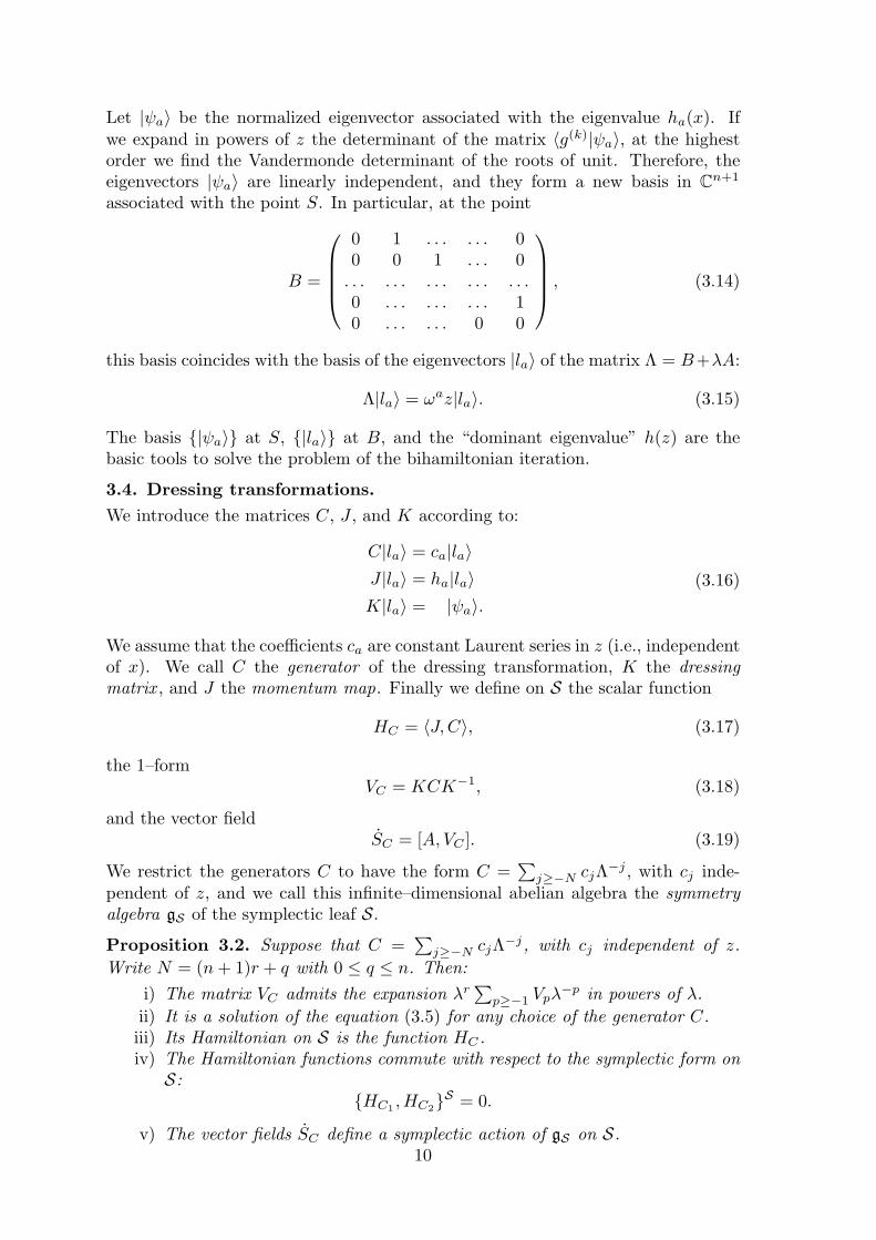
Let |ψa〉 be the normalized eigenvector associated with the eigenvalue ha(x). Ifwe expand in powers of z the determinant of the matrix 〈g(k)|ψa〉, at the highestorder we find the Vandermonde determinant of the roots of unit. Therefore, theeigenvectors |ψa〉 are linearly independent, and they form a new basis in C

n+1

associated with the point S. In particular, at the point

B =

0 1 . . . . . . 00 0 1 . . . 0. . . . . . . . . . . . . . .0 . . . . . . . . . 10 . . . . . . 0 0

, (3.14)

this basis coincides with the basis of the eigenvectors |la〉 of the matrix Λ = B+λA:

Λ|la〉 = ωaz|la〉. (3.15)

The basis {|ψa〉} at S, {|la〉} at B, and the “dominant eigenvalue” h(z) are thebasic tools to solve the problem of the bihamiltonian iteration.

3.4. Dressing transformations.

We introduce the matrices C, J , and K according to:

C|la〉 = ca|la〉

J |la〉 = ha|la〉

K|la〉 = |ψa〉.

(3.16)

We assume that the coefficients ca are constant Laurent series in z (i.e., independentof x). We call C the generator of the dressing transformation, K the dressingmatrix , and J the momentum map. Finally we define on S the scalar function

HC = 〈J,C〉, (3.17)

the 1–formVC = KCK−1, (3.18)

and the vector fieldSC = [A, VC ]. (3.19)

We restrict the generators C to have the form C =∑

j≥−N cjΛ−j , with cj inde-

pendent of z, and we call this infinite–dimensional abelian algebra the symmetryalgebra gS of the symplectic leaf S.

Proposition 3.2. Suppose that C =∑

j≥−N cjΛ−j, with cj independent of z.

Write N = (n+ 1)r + q with 0 ≤ q ≤ n. Then:

i) The matrix VC admits the expansion λr∑

p≥−1 Vpλ−p in powers of λ.

ii) It is a solution of the equation (3.5) for any choice of the generator C.iii) Its Hamiltonian on S is the function HC .iv) The Hamiltonian functions commute with respect to the symplectic form onS:

{HC1 , HC2}S = 0.

v) The vector fields SC define a symplectic action of gS on S.10

Proof.i) We remark that a Laurent series L in z contains only the coefficients of z(n+1)p

if and only if L(ωz) = L(z) for all z, where ω = e2πi

n+1 . Then from the definitionof K and from the fact that |la(ωz)〉 = |la+1(z)〉 and |ψa(ωz)〉 = |ψa+1(z)〉, wededuce that K(ωz) = K(z), so that K depends only on λ. Now we prove that

K = K0 + K1λ−1 + . . . . Indeed if K = Kmλ

m + . . . with m ≥ 1, then h(k)a =

〈gk|K|la〉 = λm〈gk|Km|la〉+ . . . . But a comparison of the degrees in z shows that〈gk|Km|la〉 = 0 for all k, a, and this implies that Km = 0. From the developmentK = K0 + K1λ

−1 + . . . it follows that K−1 = K−10 + K1λ

−1 + . . . . Finally we

have that VC = KCK−1 = cNK0ΛNK−1

0 + · · · = λ(r+1)cNK0AqK−10 + . . . , where

Λq = λAq +Bq.ii) The matrix VC has constant eigenvalues and the same eigenvectors of the oper-ator −∂ + (S + λA). Hence the two operators commute.iii) We note that J and K satisfy the equation

J = K−1(S + λA)K −K−1Kx, (3.20)

as easily checked by evaluating it on the vectors |la〉. Let S be any tangent vectorto S. Taking into account that J depends on S ∈ S both explicitly and throughK, we get:

d

dtHC =

⟨

J , C⟩

=

∫

S1

(

K−1SK + [J,K−1K], C)

dx,

where we have set K = ddtK(S + tS)|t=0. Since J commutes with C, we get

dHC

dt=

∫

S1

(

K−1SK,C)

dx =

∫

S1

(

S,KΛK−1)

dx = 〈VC , S〉.

iv) By definition of the Poisson bracket on S,

{HC1 , HC2}S = 〈VC1 , [A, VC2 ]〉 = 〈A, [VC2 , VC1 ]〉 = 0,

since the matrices VC1 and VC2 commute.v) Let ω be the symplectic form on S. The result follows from:

ω(SC , S) = ω([A, VC ], S) = 〈VC , S〉 =d

dtHC .

�

3.5. The second Hamiltonian.

Since the GD manifold is exact, we expect that the previous action is bihamiltonian,and that the function

H∗C = 〈VC , A〉 (3.21)

is the second Hamiltonian of SC . To show this result, we recall that the entries ofVC are differential polynomials of the coordinates (qa(x), pa(x)), and we introducethe matrix

V ∗C =

∂VC

∂q0(3.22)

whose entries are the partial derivatives of the entries of VC with respect to thecoordinate q0.

11

Lemma 3.4.

(1) The 1–form V ∗C , restricted to S, is exact and H∗

C is its Hamiltonian on S:

dH∗C

dt= 〈V ∗

C , S〉. (3.23)

(2) The generator SC is a bihamiltonian vector field on S, and the conjugatedfunctions HC and H∗

C are its Hamiltonians with respect to P0 and Pλ re-spectively:

SC = [A, VC ] = V ∗Cx + [V ∗

C , S + λA]. (3.24)

Proof. By deriving the equation VCx + [VC , S + λA] = 0 with respect to q0, andrecalling that

∂S

∂q0= A,

we immediately getV ∗

Cx + [V ∗C , S + λA] + [VC , A] = 0,

proving Eq.(3.24). Then we note that V ∗C can be written in the form

V ∗C =

∂VC

∂q0= [

∂K

∂q0K−1, VC ].

Finally, we compute the derivative of H∗C along S:

dH∗C

dt= 〈VC , A〉 = 〈[KK−1, VC ], A〉

= −〈[A, VC ], KK−1〉

= −〈V ∗Cx + [V ∗

C , S + λA], KK−1〉

= −〈V ∗C , (KK

−1)x + [KK−1, S + λA]〉

= 〈V ∗C , S〉 − 〈V

∗C ,KJK

−1〉

= 〈V ∗C , S〉 − 〈[

∂K

∂q0K−1, VC ],K−1JK〉

= 〈V ∗C , S〉,

since from (3.20) it is easily seen that

S = (KK−1)x + [KK−1, S + λA] +KJK−1,

and the matrices VC and K−1JK commute. �

Thus the method of dressing transformations provides a way of constructing abihamiltonian action of the symmetry algebra gS on the symplectic leaf S. Theformulas

HC = 〈J,C〉

H∗C = 〈VC , A〉

(3.25)

define the associated momentum mappings. They will be the basic objects of theabstract KP theory dealt with in the fourth paper [CFMP4].

12

4. The GD Hamiltonians and the GD equations

We complete the analysis of the previous Section by computing explicitly thecoefficients of the expansion of HC and VC in powers of λ. We fix

C = Λj (4.1)

and we denote by Hj and V j the corresponding series. We write j in the formj = (n+ 1)r + q with 0 ≤ q ≤ n. For further convenience, we formally extend thedefinition (1.11) of the GD Hamiltonians to negative integers:

Hj := (n+ 1)

∫

S1

hn+1+j dx, j ∈ Z, (4.2)

by setting h0 = 0, h−1 = 1, and h−j = 0 for j ≥ 2. Furthermore, we recall that wehave denoted by Vj the residue of the matrix V j .

Proposition 4.1. The series Hj and V j have the following expansions in λ:

Hj = λr∑

p≥2

1

λp+1H(n+1)p+q (4.3)

V j = λr∑

p≥2

1

λp+1V(n+1)p+q. (4.4)

Their coefficients Hj and Vj are related by

∂Hj

∂t= 〈Vj , S〉. (4.5)

Therefore, the restrictions to TS of the residues Vj are the differentials of the GDHamiltonians Hj.

Proof. By using the definitions of HC , J , Λ, the properties of the roots of unity,and the identity Λn+1 = λI, we get

Hj = 〈J,Λj〉

= λr〈J,Λq〉

= λr

∫

S1

n∑

a=0

ha(z)(ωaz)q dx

= λr

∫

S1

n∑

a=0

h(ωaz)(ωaz)q dx

= λr∑

l≥−1

zq−l

n∑

a=0

(ωa)q−l

∫

S1

hl dx

= λr∑

p≥−1

z−(n+1)p

∫

S1

h(n+1)p+q dx,

since∑n

a=0(ωa)q−l does not vanish if and only if l = q + p(n+ 1). The limitation

on p follows from l ≥ −1.13

Eq.(4.4) follows from the identity:

resλ(λp−rV j) = resλK(λpΛq)K−1 = resλKΛ(n+1)p+qK−1 = resλ V(n+1)p+q.

Finally, Eq.(4.5) is proved by

〈Vj , S〉 = resλ〈Vj , S〉 =

d

dtresλ〈J,Λ

j〉

=d

dtresλ (λp〈J,Λq〉)

=d

dtresλ (λpHq)

=d

dtHj .

�

By the previous results we can easily prove all the statements made in Section 1.We note that these residues form an infinite sequence bounded from below, sinceVj = 0 for j < −(2n+ 1), according to Eq.(4.4). Since the series V j obey Eq.(3.5),we conclude that the first n+1 residues V−(2n+1), . . . , V−(n+2) belong to the kernelof the first Poisson tensor P0:

[A, V−(2n+1)+q] = 0 q = 0, 1, . . . , n. (4.6)

The others verify the Lenard recursion relations

[A, Vn+1+j ] = Vj x + [Vj , S]. (4.7)

Therefore, they also verify the orthogonality relations

〈[A, Vj ], Vk〉 = 〈A, [Vj , Vk]〉 = 0 (4.8)

according to Proposition 2.2. This means that the functions Hj are in involutionwith respect to the symplectic 2–form on S, proving Proposition 1.2. Proposition1.1 easily follows from the recurrence relations (4.7) according to the Marsden–Ratiu reduction scheme.

To prove Proposition 1.3 we pass to the study of GD equations. We define theseequations as the canonical equations (1.16) on the symplectic leaf S. Let Sj denotethe corresponding vector fields on S. According to Eq.(4.5), we can write

Sj = [A, Vj ]. (4.9)

Then, if we remark that

((V j)+)x + [(V j)+, S + λA] = −((V j)−)x − [(V j)−, S + λA] (4.10)

since V j is a solution of the stationary equation (3.5), we can conclude that

[A, Vj ] =(

(V j)+)

x+ [(V j)+, S + λA], (4.11)

14

since only the coefficient of λ0 can be not zero in both sides of Eq.(4.10), and fromthe right hand side one sees that it is [A, resλ V

j ]. Therefore, we have proved that

the GD vector fields Sj admit the bihamiltonian representation

Sj = [A, Vj ] =(

(V j)+)

x+ [(V j)+, S + λA]. (4.12)

For sake of brevity, we omit to detail the study of the Hamiltonian functions asso-ciated on S to the positive parts (V j)+.

If we combine the results on the residues Vj , we arrive at the final picture of theGD hierarchy shown in Fig. 1. In this picture we have divided the infinite sequenceof residues Vj into classes of n contiguous elements. (Since V(n+1)p = δ−1

p I thesequence {V(n+1)p} is not considered.) To each residue Vj we have associated the

corresponding Hamiltonian density hn+1+j and the vector field Sj . Two consecutiven–tuples are related by the Poisson tensors P0 and P1 as shown in Fig. 1, whereր denotes the action of P0, while ց represents the action of P1. Finally, thehorizontal arrows stemming from the rightmost column represent the action of thePoisson pencil Pλ.

15

Fig. 1

00...0

ր

V−(2n+1)

V−2n

...V−(n+2)

ց

S−n

S−n+1

...S−1

←

(V −n)+(V −n+1)+...

(V −1)+

ր

h1

h2...hn

←

V−n

V−n+1

...V−1

ց

S1

S2...Sn

←

(V 1)+(V 2)+...

(V n)+

ր

hn+2

hn+3

...h2n+1

←

V1

V2...Vn

ց...

16

5. Noether theorem

We now investigate the conservation laws associated to the GD equations. Sincethese equations are Hamiltonian and their Hamiltonian functions are in involution,we expect that the latter are conserved along the flows of the GD hierarchy. Forconvenience, we collect all the Hamiltonians Hj into the single Laurent series

HGD =∑

j≥−(n+2)

Hj

zj+1, (5.1)

which we call the first GD Hamiltonian, and we write all the conservation laws inthe concise form

∂HGD

∂tj= 0. (5.2)

Since

HGD = (n+ 1)zn

∫

S1

h(z) dx, (5.3)

we expect that the dominant solution h(z) of the generalized Riccati equation

h(n+1) −n−1∑

j=0

ujh(j) = zn+1 (5.4)

verify local conservation laws of the form

∂h

∂tj= ∂xH

(j). (5.5)

We now compute the current densities H(j).

Proposition 5.1. The dominant solution h(z) of the generalized Riccati equationevolves according to the local conservation laws (5.5) defined by current densities

H(j) = 〈g(0)|(V j)+|ψ0〉. (5.6)

Proof. Let us set V = (V j)+, t = tj , and H = 〈g(0)|(V j)+|ψ0〉 for simplicity ofnotations. Then we have the relations

− |ψ0〉x + (S + λA)|ψ0〉 = h|ψ0〉

[−∂x + (S + λA),−∂t + V ] = 0.

They entail that(−∂x + (S + λA)) |φ〉 = h|φ〉 − ht|ψ0〉, (5.7)

where|φ〉 = (−∂t + V )|ψ0〉. (5.8)

Now we develop |φ〉 on the basis {|ψa〉} of eigenvectors of −∂x + (S + λA), to get|φ〉 =

∑n

a=0 ca|ψa〉, where the ca are Laurent series in z. Then (5.7) implies

n∑

a=0

(−cax|ψa〉+ caha|ψa〉) =

n∑

a=0

hca|ψa〉 − ht|ψ0〉, (5.9)

17

where h0 = h, and therefore −cax + caha = cah for all a = 1, . . . , n. Then theLaurent series ca, for a 6= 0, must fulfill the condition cax = ca(ha − h), and, sinceha − h has degree 1 in z, this implies that ca = 0. Hence |φ〉 = c0|ψ0〉, and c0 = Hfor (5.8). Therefore we have the relation |φ〉 = H|ψ0〉, that, plugged in (5.7), impliesht = Hx. �

We now elaborate on the properties of the currents H(j), to show how they canbe computed directly from the dominant solution h(z), avoiding the constructionof the matrix (V j)+. The idea is to compare the expansions of the current densitiesH(j) on the fixed basis {zj} and on the Faa di Bruno basis {h(j)}. We denote by

H+ = 〈h(0), h(1), h(2), . . . 〉 (5.10)

the module over C∞(S1) spanned by the Faa di Bruno polynomials associated withthe series h(z).

Proposition 5.2. The current densities H(j) vanish for j ≤ −1. For j ≥ 0, thecurrent density H(j) has a Laurent expansion of the form

H(j) = zj +∑

l≥1

Hjl z

−l (5.11)

and a truncated Faa di Bruno expansion

H(j) = h(j) +

j−1∑

a=0

cjah(a), (5.12)

where the coefficients cja are independent of z. Therefore the currents H(j) are theprojections

H(j) = π+(zj) (5.13)

of zj onto H+, along the splitting of the space of Laurent series in the direct sumof H+ and of the subspace of strictly negative Laurent series.

Proof. By definition, H(j) = 〈g(0)|(V j)+|ψ0〉 = 〈g(0)|V j |ψ0〉 − 〈g(0)|(V j)−|ψ0〉 =

zj − 〈g(0)|(V j)−|ψ0〉, since V 1|ψ0〉 = z|ψ0〉. Moreover, we note that (V j)− =

V j1 λ

−1 + . . . ; this implies that

−〈g(0)|(V j)−|ψ0〉 =Hj

1

z+ . . . (5.14)

since 〈g(k)|ψ0〉 = h(k) and λ = zn+1. Hence H(j) has the form (5.11).

If we put 〈g(0)|(V j)+ =∑n

i=0 aji 〈g

(i)|, then we obtain

H(j) =

n∑

i=0

ajih

(i), (5.15)

where the aji are polynomials in λ. Now we observe that for all k, i ≥ 0, λkh(i) ∈ H+,

as a consequence of the characteristic equation

λ = h(n+1) −n−1∑

j=0

ujh(j). (5.16)

18

Indeed, acting on Eq.(5.16) by the operator ∂x + h, we get

λh = h(n+2) −n

∑

j=0

u1jh

(j). (5.17)

This shows that λh ∈ H+, and so on. Therefore from Eq.(5.15) it is easily seenthat H(j) ∈ H+, proving Eq.s (5.12) and (5.13).The assertion concerning H(j), for j ≤ −1, is a consequence of the previous result.

Indeed, suppose that j < 0; then, since H(j) ∈ H+, we have H(j) =∑M

i=1 aih(mi),

with mi ≥ 0. But from (5.11) we see that H(j) has no term in zk with k ≥ 0, andtherefore ai = 0 ∀i = 1, . . . ,m. �

To see how these properties actually determine the currents H(j), let us try tocompute, for example, H(2). We start from the expansion

H(2) = h(2) + ah(1) + bh(0) (5.18)

and we compute

h(2) + ah(1) + bh(0) = (z2 + 2h1) + az + b+O(z−1) (5.19)

by using the definition of the Faa di Bruno polynomials. Therefore we have to set

a = 0, b = −2h1 (5.20)

so thatH(2) = h(2) − 2h1h

(2).

To give the general form of the currents H(j), we introduce the infinite matrix

H =

h(0) h(1) h(2) . . .

res h(0)

zres h(1)

zres h(2)

z. . .

0 res h(1)

z2 res h(2)

z2 . . .

0 res h(2)

z3 . . .

0 . . .

. . . . . . . . . . . .

(5.21)

Lemma 5.3. The currents H(j) are (up to a sign) the principal minors of thematrix H.

Proof. It is enough to develop the principal minors along the elements of the firstrow, and to remark that resH(j)z−k = 0 for k = 1, 2, . . . , j. �

This formula coincides with Eq.(5.6) when h(z) is a solution of the generalizedRiccati equation (5.4). However, it defines the current densities H(j) as differential

19

polynomials in h(z), independently of the assumption that h(z) is a solution or notof the Riccati equation. This means that henceforth we can drop this assumption,and consider the equations

∂h

∂tj= ∂xH

(j) (5.21)

for a general monic Laurent series h(z). Within this generic situation the equa-tions (5.21) will be called the full set of KP equations.The will be extensivelystudied in the fourth paper [CFMP4].

6. The second GD Hamiltonian

Now we introduce a second GD Hamiltonian H∗ according to the results on thepairing of the Hamiltonians HC and H∗

C discussed in Section 3. We consider theLaurent series

VGD =∑

j≥−(2n+1)

1

zj+1resλ V

j , (6.1)

we note that∂HGD

∂t= 〈VGD, S〉, (6.2)

and therefore we define

H∗GD = 〈VGD, A〉. (6.3)

We easily get

H∗GD =

∫

S1

h∗ dx, (6.4)

with

h∗ =∑

j≥−(2n+1)

1

zj+1(resλ V

j , A). (6.5)

Just like h(z), the function h∗(z) verifies a system of conservation laws called thereduced dual KP equations. The following remark, showing how to compute h∗

directly from h rather than from Eq.(6.5), is basic.

Lemma 6.1. The dual density h∗(z) admits the expansion

h∗(z) = 1−∑

j≥1

resH(j)

zj+1. (6.6)

Proof. From the definition of H(j) it follows immediately that

resz H(j) = resz〈g

(0)|(V j)+|ψ0〉; (6.7)

moreover, recall that H(j) = 0 for j < 0. Hence we have to prove that

(Vj , A) =

{

− resz〈g(0)|(V j)+|ψ0〉 for j 6= −1

1 for j = −120

In order to do this let us calculate

〈g(0)|(V j)+|ψ0〉 = 〈g(0)|V j |ψ0〉 − 〈g(0)|(V j)−|ψ0〉 =

= zj − 〈g(0)|(V j)−|ψ0〉. (6.8)

Therefore if j 6= −1 we have

− resz〈g(0)|(V j)+|ψ0〉 = resz〈g

(0)|(V j)−|ψ0〉 = resz〈g(0)|λ−1 resλ(V j)|ψ0〉 =

= resz〈g(0)|λ−1Vj |ψ0〉.

If we take into account that |ψ0〉 = |en〉zn + . . . , we conclude that

resz〈g(0)|λ−1Vj |ψ0〉 = 〈g(0)|Vj |en〉 = (Vj , A) j 6= −1,

since A = |en〉〈g(0)|. We are left with the case j = −1. Eq.(6.8) implies that

resz H(−1) = resz〈g

(0)|(V −1)+|ψ0〉 = resz(z−1 − 〈g(0)|(V −1)−|ψ0〉) = 1− (V1, A).

But since H(−1) = 0 we obtain that (V1, A) = 1. �

We note once again that the new expression (6.6) of h∗(z) is formally independenton any constraint on h(z), and therefore it defines the dual density h∗(z) for anymonic Laurent series h(z). The corresponding local conservation laws are calleddual KP equations. They will be studied in [CFMP4].

7. Conclusions

In this paper we have defined the GD equations as canonical equations

dqadtj

=δHj

δpa

,dpa

dtj= −

δHj

δqa(7.1)

on the symplectic manifold (1.1). Their Hamiltonians

Hj = (n+ 1)

∫

S1

hn+1+j dx (7.2)

are defined by the dominant solution

h(z) = z +∑

j≥1

hjz−j (7.3)

of the generalized Riccati equation

h(n+1) −n−1∑

j=0

uj(pa, qa)h(j) = zn+1. (7.4)

The coefficients uj(pa, qa) of this equation are computed according to the Marsden–Ratiu reduction scheme explained in Section 1. We have then remarked that theGD equations define a bihamiltonian action of the abelian algebra spanned by the

21

powers Λj on the symplectic manifold (1.1). We have accordingly written the GDequations in the bihamiltonian form

Sj = [A, Vj ] =(

(V j)+)

x+ [(V j)+, S + λA]. (7.5)

Finally, we have used this form to study the conservation laws of the GD equationsaccording to Noether theorem. We have shown that the dominant solution h(z) ofthe Riccati equation satisfies the conservation laws

∂h

∂tj= ∂xH

(j) (7.6)

and that the current densities are given by

H(j) = 〈g(0)|(V j)+|ψ0〉. (7.7)

We have also shown that these current densities can be computed directly as dif-ferential polynomials in h(z), according to the formula

H(j) = π+(zj), (7.8)

independently of the assumption that h(z) is a solution of the Riccati equation(7.4). This remark provides a natural bridge with the abstract KP theory dealtwith in the next paper [CFMP4]. Finally, we have considered the dual Hamiltoniandensity

h∗ =∑

j≥−(2n+1)

1

zj+1(resλ V

j , A). (7.9)

We have shown that it can be computed as a differential polynomial in h(z),

h∗ = 1−∑

j≥1

1

zj+1resz H

(j), (7.10)

and we have argued that it verifies a set of conjugated local conservation laws

∂h∗

∂tj= ∂xH

∗(j). (7.11)

The associated dual current densities H∗(j) will be computed in the fourth paper of

this series.

References

[CFMP1] P. Casati, G. Falqui, F. Magri, M. Pedroni, The KP theory revisited. I. A new approach

based on the principles of Hamiltonian mechanics, submitted to Comm. Math. Phys.

(1995).[CFMP2] P. Casati, G. Falqui, F. Magri, M. Pedroni, The KP theory revisited. II. The reduction

theory and Adler–Gel’fand–Dickey brackets, submitted to Comm. Math. Phys. (1995).

[CFMP4] P. Casati, G. Falqui, F. Magri, M. Pedroni, The KP theory revisited. IV. KP equations,

dual KP equations, Baker–Akhiezer and τ functions, submitted to Comm. Math. Phys.(1995).

22

[D] L. A. Dickey, Soliton Equations and Hamiltonian Systems, Adv. Series in Math. Phys,

vol. 12, World Scientific, Singapore, 1991.[GD] I. M. Gelfand, L. A. Dickey, Fractional Powers of Operators and Hamiltonian Systems,

Funct. Anal. Appl. 10 (1976), 259–273.

[GZ] I. M. Gelfand, I. Zakharevitch, Webs, Veronese curves and bihamiltonian systems,Funct. Anal. Appl. 99 (1991), 150–178.

[MR] J. E. Marsden, T. Ratiu, Reduction of Poisson Manifolds, Lett. Math. Phys. 11 (1986),

161–169.[SS] M. Sato, Y. Sato, Soliton equations as dynamical systems on infinite–dimensional

Grassmann manifold, Nonlinear PDEs in Applied Sciences (US-Japan Seminar, Tokyo)(P. Lax and H. Fujita, eds.), North-Holland, Amsterdam, 1982, pp. 259–271.

[ZS] V. E. Zakharov, A. B. Shabat, A scheme for integrating the nonlinear equations of

mathematical physics by the method of the inverse scattering problem, Funct. Anal.Appl. 8 (1974), 226–235.

23