1

THE JOINT HEDGING

AND LEVERAGE DECISION

John Gould∗

Working Paper, August 2007, v2 University of Western Australia

ABSTRACT

The validating roles of hedging and leverage as value-adding corporate strategies arise

from their beneficial manipulation of deadweight market impositions such as taxes and

financial distress costs. These roles may even be symbiotic in their value-adding effects,

but they are antithetic in their effects on company risk. To investigate both the value and

risk impacts of a joint hedging and leverage decision, this study utilises a multi-period

model for a company subject to respectively hedgeable and unhedgeable production output

price and quantity risk variables, endogenously derived deadweight costs, and the tandem

availability of risky leverage and flexible hedging control variables. While hedging and

leverage are clearly found to interact for net benefit to company value, there is no

straightforward generalisation for the relative financial riskiness of an optimal joint

hedging and leverage decision in comparison to an unhedged optimal leverage decision, an

unlevered optimal hedge decision, or an unhedged and unlevered decision; the observed

relative riskiness depends on the price level for production output, the company’s

remaining production life, and the available hedging instruments.

∗ I am grateful for the guidance and patience of my dissertation supervisors, Philip Brown and Alex

Szimayer. For advice and comments at various stages, many thanks to Bruce Grundy, Ning Gong, Kim

Sawyer, Tom Smith, Robert Webb, participants of the University of Melbourne’s Department of Finance

seminar series, Ken Clements, Robert Durand and Ross Maller. Thanks also to UWA and FIRN for

scholarship assistance during my doctoral study.

2

1. INTRODUCTION

The seemingly patent roles of corporate hedging and leverage are respectively to provide

finance and reduce financial risk. However, in getting beyond a Modigliani and Miller

(1958) irrelevance argument, their validating roles as value-adding corporate strategies

arise from their beneficial manipulation of deadweight market impositions such as taxes

and financial distress costs. Expositions in this regard include trade-off theory with respect

to leverage, and the work of Smith and Stulz (1985) with respect to hedging.

Ross (1996) took the further step of considering the interrelation of the hedging and capital

structure decisions and proposed that hedging facilitates higher optimal leverage and

thereby allows firms to access greater tax shield benefits. While hedging and leverage are

potentially symbiotic in their value-adding effects, they are antithetic in their effects on

company risk: hedging reduces a company’s financial risk ceteris paribus, but it is

indeterminate whether the optimal joint hedging and leverage decision should be

associated with increased, decreased, or unchanged financial risk compared to that when

the company is optimally unhedged and levered, or hedged and unlevered, or unhedged

and unlevered. This motivates the following research aims:

1. To provide further verification or otherwise that the value-maximising joint hedging

and leverage decision (compared to the unhedged leverage decision) is associated with

higher leverage.

2. To provide further verification or otherwise of the value-adding benefit of the joint

hedging and leverage decision (compared variously to the unhedged leverage decision,

the unlevered hedging decision, and the unhedged and unlevered decision).

3. To provide evidence as to whether the value-maximising joint hedging and leverage

decision (compared variously to the unhedged leverage decision, the unlevered hedging

decision, and the unhedged and unlevered decision) is associated with higher, lower or

generally unchanged financial risk. Five measures are used to assess financial risk: the

value of equity’s comprehensive limited liability option, equity’s value-at-risk, equity’s

beta with respect to the underlying production output’s price, and conditional and

unconditional probability of bankruptcy.

The research method utilises a multi-period model for a company subject to respectively

hedgeable and unhedgeable production output price and quantity risk variables,

3

endogenously derived deadweight costs, and the tandem availability of risky leverage and

flexible hedging control variables. With due concern for the realism of exogenous

parameter values, the model is applied as a theoretical tool to investigate both the value

and risk impacts of a joint hedging and leverage decision in the presence of deadweight

impositions in the forms of taxation, agency costs of free cash-flow, and costs of financial

distress and bankruptcy. The model’s representation of hedging and leverage control and

motivation offers favourable innovation compared with previous modelling approaches

concerned with the hedging decision in the presence of leverage (e.g. Leland (1998), Mello

and Parsons (2000) and Fehle and Tsyplakov (2005)).

It is found that an optimal (value-maximising) joint hedging and leverage strategy can

increase company value by about 3.4% compared to an unhedged optimal leverage

strategy, by about 2.2% compared to an unlevered optimal hedge strategy, and by about

3.6% compared to the company being unlevered and unhedged. Also found is that optimal

leverage is usually much higher in conjunction with optimal hedging than with no hedging,

but the relationship is observed to not purely be a matter of higher hedging facilitating

higher leverage.

At outset a jointly optimal hedging and leverage strategy markedly boosts the levels of

both hedging and leverage, compared to optimal hedging without leverage, and optimal

leverage without hedging respectively. Then as long as the price for production output is at

least rising modestly, the hedging level is largely maintained, while leverage tends to fall

due to maturing-hedge losses substituting for debt as a tax shield. For conversely weak

output price outcomes close to the unit cost of production, the ongoing operational value of

the company is low, particularly if the company is at a late stage of its production life, but

the hedge portfolio is deep in-the-money and facilitative of increased leverage driven by

pecking order roll-over of hedging-boosted debt plus tax-shielding of maturing-hedge

profit. For the hedging decision, low ongoing operational value imposes a net cost/benefit

asymmetry with respect to output price outcome, because an output price fall (below unit

production cost) will lead to abandonment/bankruptcy regardless of hedge portfolio value,1

but an output price rise will warrant continued operation and production. Given a weak

price outcome and attendant deep in-the-money hedge portfolio, high leverage and low

1 Abandonment allows the in-the-money hedge portfolio to be cashed-in instead of used to subsidise

uneconomic production.

4

ongoing operational value, the operational benefit of a subsequent output price rise is

vulnerable to the financial risk posed by the high leverage and the fact that the hedge

portfolio would lose value; that is, an output price rise actually entails adversely high risk

of bankruptcy and consequential foregone profitable production. To counter such

circumstance, reduced hedging or even a switch of the hedging decision to a speculatively

long stance increases the likelihood that the company will avoid bankruptcy in event of an

output price rise and thereby benefit from ongoing profitable production. The value-

maximising optimality of this risk-seeking behaviour arises in conjunction with fair

compensation to debt-holders and other non-equity stakeholders for limited liability risk.

The financial risk measures consequently demonstrate that, for weak output price outcomes

close to the unit cost of production, an optimal joint hedging and leverage strategy is often

more risky than any of an unhedged optimal leverage strategy, an unlevered optimal hedge

strategy, or an unhedged and unlevered strategy; but the opposite is often evident at higher

price levels. Nevertheless, overall distinction of the relative financial riskiness of optimal

joint hedging and leverage versus alternative strategies is not easily generalised and shows

dependence not only on the output price level, but also on the company’s remaining

production life and the available hedging instruments.

A generally qualitative overview of the model company’s design features and application

set-up is presented in the following Section 2 for consideration with reference to the

exacting design details provided in Appendix A. Sections 3 and 4 present and analyse the

results of application of the model, and Section 5 concludes the paper.

2. MODELLING APPROACH

I construct a multi-period model of a company, ostensibly a resource producer, subject to

hedgeable price risk and unhedgeable quantity risk for its production output. The company

has to contend with income tax, agency costs of free cash-flow, and costs of financial

distress and bankruptcy, and can manipulate its exposure to these deadweight costs via

hedging and leverage control decisions. The model is detailed in Appendix A.

The intention in the model design is to define the company’s equity and non-equity stakes

as complex, interdependent, controlled contingent claims (effectively American-style

options) on the underlying production output price and quantity random variables (tp and

5

tq respectively). Thereby an option-pricing approach can be used to value equity and non-

equity and to assess the effects of hedging and leverage control decisions.

The model company’s non-equity stakeholders are debt finance providers, hedge contract

providers, providers of production labour and equipment, and providers of direct

bankruptcy services. All non-equity stakeholders provide valuable service without

certainty of full compensation in event of bankruptcy, thereby providing equity with its

limited liability option. A prominent and important feature of the model design is that at

the beginning of every production period, equity purchases from non-equity a fairly priced

comprehensive limited liability option exercisable for the ensuing period. The periodic

upfront expense for the limited liability option will vary depending on the financial risk

being faced by non-equity each period; this expense effectively grosses together the risk

premiums that would be charged by individual non-equity stakeholders. The overall non-

equity stake is then defined to be a combination of the risk-free value of the company’s

debt plus the short value of the comprehensive limited liability option (which acts to

deduct debt’s risk premium as well as the risk premiums of all other non-equity

stakeholders from the risk-free debt valuation); the non-equity value is therefore a broader

measure than risky debt value.

Risk variables

The model company faces two sources of uncertainty: at time t , being the end of a discrete

production period of duration t∆ years, the production output for the period is an uncertain

quantity of tq units, and the price obtainable for the production output is an uncertain

amount of tp dollars per unit. The bivariate price and quantity process is assumed to be

lognormal Markovian. Hedging can only be contracted with respect to price uncertainty,

hence the price risk is hedgeable and the quantity risk is not.

The company is assumed to have uniform production periods, and periodic expected

production quantity is assumed to be independent of previous unexpected production

quantity deviations. This allows the company to be specified as blind to the history of the

stochastic component of production quantities, which advantageously allows equity and

non-equity, conditional on price and control variables, to have generalisable analytic

valuation solutions with respect to quantity uncertainty.

6

While the market price for production output (tp ) is defined as a lognormal random

variable, for the sake of model implementation it is approximated by a binomial process.

Within production periods, tp evolves by an n -step recombining binomial tree. However,

at the end of each production period the price-tree is specified as non-recombining so that

path-dependent hedging and leverage control behaviour is achievable (i.e. there are ( 1)n +

price-nodes at the end of the first production period, 2( 1)n + after period two, and so on up

to ( 1)Nn + after period N ). Correlation between production output price and quantity (ρ )

is used to represent the preference and ability of the company to adjust expected

production quantity concurrently with the trend of the market price for its output.

Control variables

The model company is specified to have N production periods for which control decisions

can be made, each of duration t∆ years. Time (t ) is denominated accordingly:

{ }0, ,2 ,...,t t t N t∈ ∆ ∆ ∆ . The company has available to it a flexible set of hedging and

leverage control variables. The periodic leverage decision allows the issue of risky zero-

coupon bonds with different maturities and individually specifiable face-values. Similarly

the periodic hedging decision allows individually specifiable hedge quantities for different

maturities. The available hedge contracts are short forwards, long put options or a ratio

combination of the two (however a negative hedge quantity would imply an ‘anti’-hedge

consisting of long forwards and/or short put options).

The computational complexity of optimising for all the possible hedging and leverage

choices available to the model company compels some limits on control behaviour. The

number of controlled production periods is limited to three ( 3N = ). The number of

possible output price outcomes for each period is limited to five (i.e. the price evolves by a

four-step binomial tree within each period). Hence there are 35 125= non-recombining

price paths for the three controlled production periods. Also the periodic leverage decision

is simplified by restricting the allowable debt maturities to a single production period.

Reiterating from Appendix A, define , 0t t ty +∆ ≥ to be the total face-value of zero-coupon

bonds issued at time t and maturing after a single production period; ,t t tx κ+ ∆ to be the

hedge quantity contracted at time t and maturing after κ production periods;

7

,0 1t t tw κ+ ∆≤ ≤ to be the ratio choice anywhere between an all-put hedge ( , 0t t tw κ+ ∆ = ) and

an all-short forward hedge (, 1t t tw κ+ ∆ = ); and , 0t t tz κ+ ∆ > to be the strike price of the put

options. The complete set of control variables is: at 0t = , one specification of

{ 0, 0,2 0,3( , , )t t tw w w∆ ∆ ∆ ; 0, 0,2 0,3( , , )t t tx x x∆ ∆ ∆ ; 0, ty ∆ ; 0, 0,2 0,3( , , )t t tz z z∆ ∆ ∆ }; at t t= ∆ , five path-

dependent specifications of { ,2 ,3( , )t t t tw w∆ ∆ ∆ ∆ ; ,2 ,3( , )t t t tx x∆ ∆ ∆ ∆ ; ,2t ty∆ ∆ ; ,2 ,3( , )t t t tz z∆ ∆ ∆ ∆ }; and,

at 2t t= ∆ , 25 path-dependent specifications of {2 ,3t tw ∆ ∆ ; 2 ,3t tx ∆ ∆ ; 2 ,3t ty ∆ ∆ ; 2 ,3t tz ∆ ∆ }.

Noteworthy is that, each period, the maturities of new hedge positions (with positive or

negative hedge quantities) may overlap with previously established hedge positions so as

to increase or decrease the overall hedge position for any particular maturity.

Although the company does not have an explicit option to abandon, it does have the ability

to force bankruptcy (and hence abandonment) via an ‘extreme’ hedging or leverage control

decision which radically increases financial risk and thereby triggers immediate

bankruptcy. Such voluntary bankruptcy will not necessarily result in loss for non-equity

stakeholders and may be desirable when the output price drops so low as to make ongoing

production economically unviable.

2.1. Leverage and hedging imperatives

The modelling approach developed for this study is attractive for its inclusion of a range of

features that allow the model company to be controlled in respect of several theoretical

imperatives. Modigliani and Miller’s (1958) demonstration of the irrelevance of capital

structure under the condition of a ‘perfect market’ dictates that acceptance of capital

structure relevance must presume deviation(s) from the perfect market condition. Likewise

must be the presumption for acceptance of corporate hedging relevance. To this effect, the

model company is established as subject to: deadweight costs (taxation) of income

attributable to equity; deadweight costs of financial distress; deadweight costs of

bankruptcy; and deadweight costs of free cash-flow.

The assumption of asymmetric corporate taxation, entailing tax deductibility of interest

payments to lenders but (some degree of) non-deductibility of income attributable to

equity, potentially allows firms to add value by using debt finance to reduce their corporate

tax burdens. The actual value benefit to any firm of debt finance as a tax shield depends on

the corporate tax rate and system (generally classical versus imputation systems), and the

8

personal tax rates for debt and equity income for a ‘marginal’ investor indifferent between

debt and equity income.2 The ‘effective’ rate of tax shielded by an additional unit of

corporate debt derives from the additional post-tax value of attributing a dollar of pre-tax

corporate income to the marginal investor as an interest payment for debt finance as

opposed to a dividend plus capital gain return for equity finance. Under a classical tax

system this marginal tax advantage of debt finance over equity finance is:

(1 ) (1 )(1 )PD C PEA τ τ τ= − − − −

where Cτ is the marginal expected corporate tax rate, and PDτ and PEτ are respectively the

personal tax rates on debt and equity income for the marginal investor. How equity income

is split between dividends and capital gains and the investor’s preferences for realising

capital gains add complexity to the determination of PEτ .

For a dividend imputation tax system, corporate taxation can be claimed by (some)

investors as a credit for personal taxation on grossed-up dividend income.3 As such the

combined corporate and personal tax burden for equity finance depends on the firm’s

dividend payout ratio (θ ), the imputation credit ratio (ω ), and the ability of investors to

access the face-value of dividend imputation credits; defining ν as the marginal investor’s

valuation ratio for imputation credits, the marginal tax advantage of debt finance is:

( ) [ ]( ){ }( ) ( )(1 ) (1 )(1 ) 1 1 (1 ) 1imputation PD C PE capital gains C PE dividendsA τ θ τ τ θ ων τ τ= − − − − − + − − − .

Miller (1977) argued that firms, desirous of debt finance over equity finance, will act

competitively and increase the interest rates they offer to attract more lenders until the

marginal investor offers no tax benefit for debt over equity (i.e. for whom

,( ) 0C beforedebt financeA τ ≤ for all firms). Consequently lenders capture all of the corporate tax

shield benefit of debt and, although an equilibrium aggregate level of debt across all firms

obtains, individual firms receive no benefit from their capital structure choices.

2 Although firms and investment intermediaries can take debt and equity stakes in each other, the marginal

investor is an individual amongst all of the individuals that are the ultimate suppliers of all debt and equity

finance (n.b. government can arguably be considered to also be amongst these individuals).

3 Grossed-up dividend value equals the cash dividend amount plus the associated imputation credit.

9

DeAngelo and Masulis (1980) counter-argued Miller (1977) by considering the availability

of non-debt tax shields combined with the potential for excessive tax shields to go

unutilised. Non-debt tax shields like depreciation expenses and carry-forward losses will

arise in conjunction with the normal operations of firms and will therefore tend to be

available to reduce taxable income ahead of the discretionary issue of debt for tax shield

purposes. Furthermore, as a generalisation, tax law restricts the realisation of the nominal

value of tax shields when taxable income is negative (possibly in association with

bankruptcy). Thus, for individual firms, after firstly allowing for non-debt tax shields to be

claimed against income, the marginal expected benefit of debt as a tax shield may decline

rapidly as debt level increases; since higher debt makes an earnings loss (negative taxable

income) more probable and tax shields less valuable at the margin. Such considerations

will cause individual firms to limit their demand for debt finance such that the aggregate

may potentially be satisfied by lenders up to a marginal investor who does offer a tax

benefit for debt over equity (i.e. for whom ,( ) 0C beforedebt financeA τ > for at least some firms).

The critical issue is whether the supply of investors that satisfy ,( ) 0C beforedebt financeA τ > for at

least some firms is sufficient for all firms to reach their individual leverage equilibriums

before Miller’s (1977) aggregate equilibrium is reached.

The actual process by which any tax benefit of debt financing is capitalised into the value

of a firm has two opposing elements: the cash expected to be saved from corporate tax (i.e.

higher expected post-corporate tax, pre-financing cash-flows); and a market cost for debt

finance that has been grossed-up to reflect the marginal investor’s personal tax penalty for

debt income relative to equity income (assuming PD PEτ τ> ).4 To establish whether there is

any tax benefit to be had from debt financing, it is problematic that the marginal investor’s

characteristics are not specifically ascertainable. Additionally confounding is that the

relevant corporate tax rate is the marginal expected rate after consideration of all in-place

and expected tax shields. An individual firm’s marginal expected corporate tax rate will be

an idiosyncratic function of the convolutions of tax law, such as carry-forward and carry-

back tax shield provisions for earnings losses, applied to past and expected future earnings.

4 As a generalisation of tax law, relatively favourable personal tax conditions for capital gains mean that the

overall personal tax rate for equity income can be expected to be lower than for debt income.

10

Under the taxation regime established for the model company, so long as the company is

not bankrupt, positive earnings before tax is subject to the full corporate tax rate (α ),

while negative earnings before tax is subject to a partial corporate tax rate (λα , where

0 1λ≤ ≤ represents the claimability of a tax refund in event of an earnings loss). That is,

instead of allowing carry-forward or carry-back of earnings losses as tax shields, the

model’s taxation regime gives the company a partial but immediate tax benefit (refund) for

an earnings loss. The tax shields that are available each production period are simply the

period-specific expenses used to calculate earnings. The resulting model set-up is such that

the company’s marginal expected corporate tax rate arises and adjusts endogenously

through time in respect of the risk variables and in response to control decisions.

The model company’s primary non-debt tax shield is total production costs. The company

can be considered to lease (for operation) rather than own the necessary physical assets for

production, hence depreciation tax shields are implicitly included in total production costs.

Hedging outcomes net of transaction costs are also included in taxable earnings. Otherwise

the company’s debt tax shield is incorporated as part of a broader expense calculated each

period and symbolised by (,t t t ty Y+∆ − ) at time t , where: ,t t ty +∆ is the face-value of newly

issued debt (with maturity of a single production period); and tY , termed the risky measure

of new debt proceeds, equals the short value of equity’s comprehensive limited liability

option ( 0tO + ≤ ) plus the risk-free value of the newly issued debt with personal tax penalty

adjustment. Effectively the interest expense for debt is calculated and tax deducted

immediately upon issue in combination with the expense for the limited liability option

each period.

The effective marginal debt tax shield rate (A ) for a firm with high demand for tax shields

(i.e. for which the marginal expected corporate tax rate equals the full corporate tax rate,

Cτ α= ) indicates the upper limit for that part of the full corporate tax rate that effectively

gets shielded by debt finance relative to equity finance after lenders are compensated for

their personal tax penalty. Defining ( )CA Aα τ α= = , the part of the full corporate tax rate

that is converse to Aα (i.e. ( )Aαα − ) is that part of the full corporate tax rate shield that

gets passed on to lenders as a higher rate of return in compensation for their personal tax

penalty. Dictating the model company to be valued on a pre-personal tax on equity basis,

11

the company’s proceeds from issuing debt are adjusted for debt’s personal tax penalty via

the risk-free debt valuation component of the risky measure of new debt proceeds:5

[ ], 1 ( )

( )t t t

t t r t

y AY O

e Aα

α

αα

+∆+ ∆

− −= +

− −

where r is termed the risk-free interest rate but is more correctly described as the pre-

personal tax risk-free rate of return for equity.

As a result of the model’s overall taxation set-up, no direct assumption is made about

whether there will be any net tax benefit from any level of debt finance at any stage of the

company’s operations. The net tax benefit to be had from each incremental dollar of debt

finance, whether positive, zero or negative, arises endogenously, but is, however, affected

by the exogenous choices for the λ , α and Aα parameters. A higher value for the

claimability of a tax refund for a loss (λ ) increases the marginal expected corporate tax

rate and makes debt finance more attractive (as a result of the tax rate for a loss being

higher, meaning a higher tax refund in event of a loss and lower potential financial penalty

from being highly levered); similarly a higher value for the full corporate tax rate (α )

makes debt finance more attractive (for its tax shield effect); whereas a higher value for the

personal tax penalty against debt’s corporate tax shield rate ( Aαα − ) increases the cost of

debt finance and makes it less attractive.

Due to the tangle of details routinely associated with tax law, an empirically appropriate

value for α may be less than perfectly manifest. For example, under the US classical tax

system the federal corporate tax rate varies across rising earnings bands to become a flat

rate of 35% for earnings above a relatively modest threshold of about $18 million;

additionally more irksome is the raft of different state corporate tax rates that can apply

(but which are deductible at the federal level). Under an imputation tax system, additional

empirical ambiguity arises because it is appropriate to adjust α according to dividend

payout ratio (θ ), the imputation credit ratio (ω ), and the marginal investor’s imputation

credit valuation ratio (ν ):

5 The risk-free debt valuation component of risky new debt proceeds (t t

Y O +− ) is adjusted for debt’s personal

tax penalty by solving the risk-free valuation inclusive of a tax penalty charge against the income earned by

the lender: [ ]{ }, ,( ) ( ) ( ) r t

t t t t t t t t t tY O y y Y O A eαα − ∆

+ +∆ +∆ +− = − − − − .

12

(1 ) (1 )imputationα θ α θ ων α= − + − .

There is also considerable empirical ambiguity about what are appropriate values for λ

and Aα . The intention for λ is to reflect, on average, corporate tax law provisions for the

carry-forward and carry-back of earnings losses for tax shield purposes. Under the US tax

system an earnings loss can be carried backward for up to three years and forward for up to

15 years. Hence a US company that is generally profitable suffers relatively little

opportunity cost for excess tax shields in event of an earnings loss, which tends to support

a relatively high value for λ ; but in turn this may encourage more aggressive use of tax

shields (i.e. leverage), making earnings losses more likely and increasing the expected

opportunity cost of excess tax shields, thereby lowering the appropriate value for λ .

Evidence on historic values for A for the US tax system was obtained by Graham (1999)

using a simulation procedure and meticulous application of historic tax laws to estimate

marginal expected corporate tax rates for individual firms on the COMPUSTAT database

for each year from 1980 to 1994. This was done with careful consideration of non-debt tax

shields for both a before and after debt financing basis. Each year’s median value for the

marginal expected corporate tax rate after non-debt tax shields but before debt financing

was consistently at or very close to the top corporate tax rate (i.e. ,C beforedebt financeτ α≈ ).

With further careful assumptions about the marginal investor’s personal tax rates, Graham

also estimated the yearly marginal tax advantage of debt finance for individual firms

before any debt finance ( ,( )C beforedebt financeA τ ) and after actual historic debt finance

( ,( )C after debt financeA τ ). The median value of ,( )C beforedebt financeA τ ranged between 0.075 and

0.102 for the years 1982 to 1994, but was considerably lower, though still positive, for

1980 and 1981; this indicates a generally consistent and substantial tax advantage for debt

finance. Furthermore, the median value of ,( )C after debt financeA τ ranged between -0.002 and

0.018 for the years 1986 to 1994, and was 0.012 for 1980 and 1981, but was notably higher

for 1982 to 1985; this is generally consistent with a trade-off theory explanation being that

firms take on debt finance up to the point where the marginal tax benefit is zero or, due to

offsetting marginal disbenefits, slightly positive.6

6 That the trade-off equilibrium for leverage should occur when the marginal tax benefit of debt is zero or

slightly positive is consistent with Miller’s (1977) suspicion that the expected bankruptcy cost disbenefit of

13

Trade-off theory suggests that firms will individually take on debt finance up until the

marginal expected benefit equals marginal expected disbenefits. The most prominently

espoused disbenefit to firms of higher debt levels is higher likelihood of suffering costs of

financial distress and bankruptcy.7 Andrade and Kaplan (1998) investigated a sample of

firms that became financially distressed after undertaking highly leveraged transactions

(HLTs, i.e. capital restructuring that greatly increased leverage) during the 1980s. To

isolate financial distress from economic distress, Andrade and Kaplan limited their sample

to firms that maintained positive operating margins while financially distressed. They

estimated the costs of financial distress to be about 10% to 20% of pre-distress firm value.

For comparison’s sake, in contrast to the broad costs of financial distress, the direct costs

of bankruptcy were estimated by Weiss (1990) to be 3.1% of firm value on average. While

these cost estimates clearly represent a considerable ex-post encumbrance, the probability

of a typical firm experiencing financial distress or bankruptcy is small, and thus so are the

expected costs of financial distress and bankruptcy.

For the model company, occurrence of financial distress or bankruptcy, as distinct from a

state of solvency, is signalled by the value of periodic free cash-flow ( tF ), being the

overall net cash-flow from operations, hedging, debt and taxation resulting ultimately from

control decisions and the outcomes for tp and tq . Positive or zero free cash-flow is a state

of solvency, in which case the free cash-flow is paid out as a dividend to equity (i.e. it is

assumed that the company does not retain any earnings or any capital from the issue of

debt). Negative free cash-flow signals financial distress and necessitates new equity

finance (i.e. a negative dividend, which can be conceptualised as a rights issue).

Bankruptcy (and consequential liquidation) occurs when the free cash-flow shortfall is so

debt is a minor concern. Specifically Miller described the capital structure trade-off between tax gains and

bankruptcy costs as looking like “the recipe for the fabled horse-and-rabbit stew - one horse and one rabbit”!

7 Financial distress entails difficulty or inability to satisfy financial obligations in a timely manner. There can

be several mechanisms by which financial distress reduces the value of a firm: trade creditors, customers and

employees who have a stake in the firm as a going concern and fear bankruptcy may behave more

restrictively towards the firm; managerial time and resources will be diverted to the financial predicament;

some debt covenants may be broken leading to financial or operational penalties; profitable investment

opportunities may have to be foregone since new finance will be more difficult to obtain; and valuable assets

may have to be sold at depressed prices. These deadweight costs of financial distress will also generally

apply once an official state of external administration or bankruptcy is declared. There will also be additional

explicit (direct) legal and administrative costs associated with bankruptcy.

14

large that the required amount of new equity finance cannot be justified by the ongoing

equity value ( tE + ). By this method the states of financial distress and bankruptcy are

determined endogenously.

In event of negative free cash-flow ( 0tF < ), for the model company to be able to access

future earnings potential it must finance the free cash-flow shortfall ( tF− ); in such case the

trade-off optimum for new debt finance takes into account the costliness of resorting to

new equity finance. Note that free cash-flow includes cash-flow from new debt finance but

excludes cash-flow from new equity finance. The model is set up to appeal to Myers’

(1984) pecking order theory to the extent that endogenous resorting to new equity finance

is defined to signify financial distress, and accordingly a financial distress cost is applied

with such occurrence. This pushes the leverage trade-off optimum more in favour of debt

finance to cover a free cash-flow shortfall and makes new equity finance more of a last

resort. The financial distress cost is applied as a factor ( 0γ ≥ ) of the free cash-flow

shortfall so that equity-holders must invest (1 )tF γ− + to finance a free cash-flow shortfall

of tF− so as to access an ongoing equity value worth tE + . The financial distress cost

( tFγ− ) is a penalty to equity that represents, for instance, the direct transaction costs of the

new equity issue and the operational difficulties that may arise when stakeholders fear

imminent bankruptcy; or, more characteristic of pecking order theory, it can represent the

costs of assuaging principal-agent information asymmetry.

The endogenous occurrence of bankruptcy for the model company represents equity

exercising its limited liability option to refuse new equity finance and liquidate the

company. This will occur when the required amount of new equity finance inclusive of

financial distress costs ( (1 )tF γ− + given 0tF < ) is greater than the company’s ongoing

equity value (i.e. when /(1 )t tF E γ+< − + ). In this case the company is liquidated for the

current period’s operating profit and net payoff of maturing hedge contracts, plus the net

market value of any non-maturing hedge contracts, minus the face-value of outstanding

debt factored up by a bankruptcy cost rate (b ). A positive liquidation cash-flow is a

remainder after the claims of all non-equity stakeholders have been satisfied in full;

positive liquidation cash-flow is taxed and then paid as a liquidating dividend to equity. A

negative liquidation cash-flow indicates a combined loss suffered by non-equity

stakeholders due to their claims being partly or wholly unpaid.

15

It is assumed that only debt-holders are willing to pay anything for bankruptcy

proceedings, hence the model’s bankruptcy cost is applied as a factor (b ) of the face-value

of outstanding debt. Consequently if there is no outstanding debt, there will be no

bankruptcy cost. And because the conditions of financial distress and bankruptcy cannot

occur concurrently for a production period, there is no financial distress cost applied with

the occurrence of bankruptcy. Thus it may be desirable to set the bankruptcy cost rate to a

level that incorporates some degree of financial distress cost associated with bankruptcy.

Nevertheless, because the financial distress cost rate lowers the level of free cash-flow

shortfall at which bankruptcy occurs, there is an effective financial distress opportunity

cost associated with bankruptcy (i.e. the company gets liquidated ‘too early’ at a free cash-

flow shortfall of /(1 )tE γ+ + instead of tE + ).

Deadweight financial distress and bankruptcy costs cause an asymmetry in the possible

financial outcomes for a firm such that bad future financial states of the world will be more

significantly value-destroying than good future states will be value-enhancing. Hedging, in

essence, reduces the variability of future aggregate cash-flows and thereby reduces the

likelihood of both good and bad future financial states (i.e. reduces financial risk). This

reduces the firm’s exposure to financial outcome asymmetry and provides a net increase in

value equal to the reduction in expected financial distress and bankruptcy costs. This

source of added-value from hedging was proposed by Smith and Stulz (1985). Hedging’s

effect on financial risk means that it can also be used to ramp-up leverage’s trade-off

equilibrium. Ross (1996) proposed that hedging facilitates higher optimal leverage and

thereby allows firms to access greater tax shield benefits. Ross explained that hedging

“enables the firm to substitute tax-benefitted risk, in the form of leverage, for non-tax-

benefitted risk”. Graham and Rogers (2002) were the first to empirically investigate the

hedging and leverage decisions jointly and, in favour of Ross’s proposition, they found that

firms do hedge to increase debt capacity and that this behaviour is tax motivated.

Additionally their evidence indicated that firms also hedge in response to large expected

financial distress costs. Graham and Rogers concluded that “a complete modelling of

corporate debt policy should control for the influence of hedging decisions”.

In addition to its role as a tax shield, another avenue by which debt can add value is as a

shield against agency costs. This potential benefit arises out of Jensen’s (1986) free cash-

flow theory which posits that the cash-flow discipline required to sustain high leverage

means that there is less free cash-flow available for self-interested managers to squander.

Myers (2001) suggested that, with hindsight, it seems clear that the 1980s spate of

16

leveraged buyouts was a manifestation of Jensen’s free cash-flow problem. In reflection of

this, the model company is subject to a deadweight agency cost applied as a factor

( 0 1a≤ ≤ ) of positive free cash-flow; hence under condition of solvency (i.e. positive or

zero free cash-flow, 0tF ≥ ), management misappropriates an amount equal to taF , and the

dividend paid out to equity equals (1 ) ta F− .

In summary, the model company serves as a framework by which several prominent

corporate finance theories can interact and counteract. Fundamentally it allows playing-out

of the trade-off theory of leverage with deference to pecking order theory in regard to

dependence on new equity finance. Very importantly the trade-off set-up is augmented to

allow playing-out of the effects of hedging: directly on expected financial distress and

bankruptcy costs as per Smith and Stulz (1985); and in feedback to trade-off leverage

capacity as per Ross (1996). Additionally the trade-off set-up is subject to a deadweight

cost of positive free cash-flow as per Jensen’s (1986) free cash-flow theory. Under sway of

these theoretical influences, the model company’s available control behaviour appeals to

realism via multi-period incorporation of risky leverage and flexible hedging control

variables subject to hedgeable and unhedgeable risk factors.

2.2. Valuation method

Assuming a complete market for the output price and perfectly diversifiable production

quantity risk, risk-neutral valuation is used to obtain market values for equity and for non-

equity’s combined debt plus short limited liability option position. The valuation process

works backwards through the binomial price-tree with the production quantity risk

incorporated analytically into the valuations at each price-node.

Further to assuming that the model company will operate (while not bankrupt) for three

consecutive controlled production periods, it is assumed that the company has presently

completed an uncontrolled (i.e. without hedging or leverage) production period, and will

operate (if not previously bankrupted) for a fourth and final production period

uncontrolled. The presently (time 0t = ) completed production period provides the

company with current income which motivates an immediate tax-reducing capital

restructure (because the interest expense for leverage is specified within the model as tax

deductible in advance). The fourth production period provides an output ‘bank’ from

17

which production can be brought forward or to which production can be delayed;8

consequently it is necessary to specify a total output resource (R ). The binomial price-tree

process applied for the three controlled production periods is assumed to continue for the

fourth period.

The valuation process requires predetermined valuations at the terminal price-nodes. To

this end it is assumed that the output resource remaining to be produced in the final

uncontrolled production period is deterministic on the price-path-specific expected

production quantities for the prior three controlled production periods. The binomial price-

tree is four-step recombining within production periods and non-recombining between

production periods. Hence there are 125 path-specific price-nodes at the end of the third

controlled production period. An ongoing equity value for each of these 125 price-nodes at

end-of-period three (start-of-period four) is calculated according to an assumed all-equity

payoff exposure for period four:

[ ] ( )4

3

3 ( 1) 3 41

ˆ ˆmax 0, E | E ( ) 1 (1 ) It

r tt i t i t i t t t p c

i

E e R q p p c αλ α λ∆

− ∆∆ + − ∆ ∆ ∆ ∆ ∆ >

=

= − − − − − ∑

where: E [ ]t ⋅ is the risk-neutral expectation operator; the indicator function, Ilogical statement ,

equals one if the logical statement is true and zero otherwise; R is the total output resource

for the three controlled and final uncontrolled production periods; r is the annual,

continuously compounding risk-free interest rate; c is the total production cost per unit of

expected production quantity; α is the corporate tax rate; and λ is the claimability of a

tax refund in event of negative earnings.

For model set-up it has been assumed that deviation in production quantity from

expectation (conditional on price outcome) for a production period does not impact on

future production quantity expectations. For the context of a resource producer with a

limited resource, the quantity risk does not represent variability of production capacity or

efficiency, but rather represents variability of resource quality (e.g. ore concentration)

during a production period, albeit with no implication for expectations of resource quality

for future production periods. Hence the output resource remaining for fourth period

8 Specification of the correlation between production quantity and output price (ρ ) determines how the

company shifts production through time.

18

production is calculated by subtracting from the initial total output resource (R ) the (price-

path conditional) expected rather than actual production quantities for the preceding three

controlled production periods ( [ ]3

( 1)1E |i t i t i ti

q p− ∆ ∆ ∆=∑ ).

Having calculated the 125 path-specific end-of-period three ongoing equity values (3 tE ∆ + ),

and given the 25 path-specific sets of control variables applicable to period three

{ 0,3 ,3 2 ,3( , , )t t t t tw w w∆ ∆ ∆ ∆ ∆ ; 0,3 ,3 2 ,3( , , )t t t t tx x x∆ ∆ ∆ ∆ ∆ ; 2 ,3t ty ∆ ∆ ; 0,3 ,3 2 ,3( , , )t t t t tz z z∆ ∆ ∆ ∆ ∆ }, 9 it is

possible to calculate 125 corresponding price-conditional expected equity and non-equity

valuations for the instant immediately prior to end-of-period three. These expected

valuations, 2 3 3ˆ [ | ]t t tE p∆ ∆ − ∆Ε and 2 3 3 3

ˆ [ | ]t t t tD O p∆ ∆ − ∆ − ∆Ε + , are respectively obtained using

equations (A.1) and (A.2) in Appendix A, where: 3 tE ∆ − is the total equity value

immediately prior to any dividend payment or new equity finance; 3 2 ,3t t tD y∆ − ∆ ∆= is the

risk-free debt value immediately before settlement of the maturing debt; and 3 tO ∆ − is the

short payoff value of the expiring comprehensive limited liability option. The price-

conditional expectations are obtained analytically with respect to production quantity

uncertainty and take into account the condition of the company as variously solvent,

financially distressed or bankrupt across the spectrum of possible quantity production

outcomes. The discounted unconditional expectations then give the 25 path-specific end-

of-period two ongoing equity and non-equity values. These valuations, 2 tE ∆ + and

2 2t tD O∆ + ∆ ++ , are respectively obtained using equations (A.3) and (A.4) in Appendix A,

where: 2 tE ∆ + is the ongoing equity value immediately after any dividend payment or new

equity finance and implicitly conditional on bankruptcy having not occurred;

2 2 ,3r t

t t tD y e− ∆∆ + ∆ ∆= is the risk-free value of newly issued debt; and 2 tO ∆ + is the short initial

value of the newly contracted comprehensive limited liability option.10

9 There are 25 path-specific price-nodes at end-of-period two, for each of which unique control decisions can

be made entering into period three.

10 Recall that each production period’s leverage control decision has been restricted to the use of debt with a

maturity of only a single period, and that, by model design, equity’s comprehensive limited liability option

must be newly contracted each period with a maturity of only a single period.

19

Now with the 25 path-specific values for 2 tE ∆ + and 2 2t tD O∆ + ∆ ++ , and given the five path-

specific sets of control variables applicable to period two { 0,2 0,3 ,2 ,3( , , , )t t t t t tw w w w∆ ∆ ∆ ∆ ∆ ∆ ;

0,2 0,3 ,2 ,3( , , , )t t t t t tx x x x∆ ∆ ∆ ∆ ∆ ∆ ; ,2t ty∆ ∆ ; 0,2 0,3 ,2 ,3( , , , )t t t t t tz z z z∆ ∆ ∆ ∆ ∆ ∆ }, the 25 path-specific values

for 2 2ˆ [ | ]t t tE p∆ ∆ − ∆Ε and 2 2 2

ˆ [ | ]t t t tD O p∆ ∆ − ∆ − ∆Ε + can be calculated (using again equations

(A.1) and (A.2) in Appendix A), and thence the five path-specific values for tE∆ + and

t tD O∆ + ∆ ++ obtain (using again equations (A.3) and (A.4) in Appendix A). Note that the

maturing hedge control variables {0,2 ,2( , )t t tw w∆ ∆ ∆ ; 0,2 ,2( , )t t tx x∆ ∆ ∆ ; 0,2 ,2( , )t t tz z∆ ∆ ∆ } are

relevant to the valuation process for period two, as are the non-maturing hedge control

variables { 0,3 ,3( , )t t tw w∆ ∆ ∆ ; 0,3 ,3( , )t t tx x∆ ∆ ∆ ; 0,3 ,3( , )t t tz z∆ ∆ ∆ } via their effect on the liquidation

cash-flow in event of bankruptcy at end-of-period two.

Continuing in the same vein, 0E + and 0 0D O+ ++ obtain. With the further assumption of an

uncontrolled production period having just been completed at time 0t = with unresolved

production quantity uncertainty, the values 0 0ˆ [ | ]t E p−∆ −Ε and 0 0 0

ˆ [ | ]t D O p−∆ − −Ε + obtain

with 0 0D − = due to the production period being uncontrolled. The combined value of

0 0 0ˆ [ | ]t E O p−∆ − −Ε + is then used to represent an all-equity valuation that encompasses the

impacts of each price-path-dependent control decision going forward.

2.3. Model application

To determine the valuation and financial risk differentiations for the model company

between a joint hedging and leverage decision, an unhedged leverage decision, an

unlevered hedging decision, and an unhedged and unlevered state, six strategies for control

behaviour are specified. Each strategy has the common aim of maximising the value of the

company (signified by 0 0 0ˆ [ | ]t E O p−∆ − −Ε + ), but with different limitations on the available

control variables. The control decision to abandon (voluntarily liquidate) the company is

made available to all control strategies by always allowing an extreme hedge choice of

short forward 10 million units at the start of each production period (irrespective of

whether an individual control strategy specifies availability of hedging control). The six

control strategies are:

20

1. Unlevered, unhedged strategy, which requires optimisation of the abandonment

decision, with the absence of leverage or hedging.

2. Levered, unhedged strategy, which requires joint optimisation of the abandonment

decision, and the 31 price-path-specific leverage control variables ( ,t t ty +∆ ), with the

absence of hedging.

3. Unlevered, forward-only hedge strategy, which requires joint optimisation of the

abandonment decision, and the 38 price-path-specific hedge quantity control variables

( ,t t tx κ+ ∆ ) with the short forward versus put option ratio choice set to all-forward

( , 1t t tw κ+ ∆ = ), with the absence of leverage.

4. Unlevered, put-only hedge strategy, which requires joint optimisation of the

abandonment decision, and the 76 price-path-specific hedge quantity and put option

strike price control variables (38 each of ,t t tx κ+ ∆ and ,t t tz κ+ ∆ ) with the short forward

versus put option ratio choice set to all-put option ( , 0t t tw κ+ ∆ = ), with the absence of

leverage.

5. Levered, forward-only hedge strategy, which requires joint optimisation of the

abandonment decision, the 31 price-path-specific leverage control variables (,t t ty +∆ ),

and the 38 price-path-specific hedge quantity control variables ( ,t t tx κ+ ∆ ) with the short

forward versus put option ratio choice set to all-forward ( , 1t t tw κ+ ∆ = ).

6. Levered, forward+put hedge strategy, which requires joint optimisation of the

abandonment decision, and all 145 price-path-specific leverage and hedging control

variables (31 of ,t t ty +∆ , and 38 each of ,t t tx κ+ ∆ , ,t t tw κ+ ∆ and ,t t tz κ+ ∆ ).

Measures of leverage, hedging and financial risk

For different exogenous parameter scenarios, the six control strategies are assessed for

differences in optimised leverage and hedging levels, financial risk, and valuation for the

model company. Appendix B details the formulations of the leverage, hedging and

financial risk measures.

21

The leverage measure (t+l ) is the risk-free valuation of newly issued bonds

( ,r t

t t t tD y e− ∆+ +∆= ) divided by ongoing equity value (tE + ). Recall that although the model

accommodates risky debt, debt’s risk premium is indistinctly incorporated into the

comprehensive limited liability option purchased by equity from all non-equity

stakeholders. For this reason t+l is calculated using risk-free debt valuation and will

therefore tend to be a high measure in comparison to empirical leverage observations based

on market or book values of debt.

Naive measures of the extent of hedging consider only the contracted price and quantity of

individual hedge positions in a firm’s overall hedge portfolio. An alternative approach is to

calculate the delta of the hedge portfolio (i.e. the sensitivity of the hedge portfolio value

with respect to the underlying asset price) which intrinsically takes into account any non-

linearity of the individual hedge positions. The extent of hedging is then indicated by the

ratio of the hedge portfolio delta to the quantity of underlying asset to which the firm has

financial exposure. This measure is here termed the hedge-delta ratio (th + ) and is

effectively equivalent to the delta-percentage measure defined by Tufano (1996). Because

the model company has available to it the use of non-linear hedge contracts (specifically

put options), the hedge-delta ratio is considered an appropriate hedging measure. The

model company’s hedge portfolio delta is calculated as a discrete measure in accordance

with the assumed binomial price process; the formulation for the discrete binomial process

delta of individual hedge positions ( , : , /t t t tx X pτ τ κ τ τ κ+ ∆ + ∆∆ ∆ ) is given in Appendix B.

Summing the individual hedge position deltas to give the hedge portfolio delta, the hedge-

delta ratios ( th + ) for each of the company’s three controlled production periods are thus

specified to be:

0, 0:0, 0,2 0:0,2 0,3 0:0,30 0 0

0

t t t t t tx X x X x Xp p p

hR

∆ ∆ ∆ ∆ ∆ ∆

+

∆ ∆ ∆− + + ∆ ∆ ∆ = ,

[ ]0,2 :0,2 0,3 :0,3 ,2 : ,2 ,3 : ,3

0E |

t t t t t t t t t t t t t t t tt t t t

t

t t

x X x X x X x Xp p p p

hR q p

∆ ∆ ∆ ∆ ∆ ∆ ∆ ∆ ∆ ∆ ∆ ∆ ∆ ∆ ∆ ∆∆ ∆ ∆ ∆

∆ +∆ ∆

∆ ∆ ∆ ∆− + + + ∆ ∆ ∆ ∆ =−

,

22

[ ] [ ]0,3 2 :0,3 ,3 2 : ,3 2 ,3 2 :2 ,3

2 2 22

0 2 2ˆ ˆE | E |

t t t t t t t t t t t t tt t t

t

t t t t t

x X x X x Xp p p

hR q p q p

∆ ∆ ∆ ∆ ∆ ∆ ∆ ∆ ∆ ∆ ∆ ∆ ∆∆ ∆ ∆

∆ +∆ ∆ ∆ ∆ ∆

∆ ∆ ∆− + + ∆ ∆ ∆ =− −

.

The denominator of the hedge-delta ratio is specified to be the remaining resource

expected to be produced for all future production periods (i.e. the total remaining

underlying asset). An alternative approach would be to specify that the denominator equal

the expected production quantity for only the remaining controlled (hedgeable) production

periods (i.e. excluding the uncontrolled fourth production period), which would match the

production time-frame of the denominator with the maximum hedge maturity time-frame

of the numerator. However, the delta measure indicates immediate hedge portfolio

sensitivity to underlying price irrespective of specific hedge contract maturities or the time-

frame for the underlying price exposure.11 Thus it is reasonable and preferable that the total

remaining production resource be incorporated in the hedge-delta ratio so as to indicate the

extent of hedging for the entire spot position.12

Five measures of financial risk are considered, the first being a limited liability risk

measure equal to the value of equity’s comprehensive limited liability option divided by

ongoing equity value ( /t tO E+ +− ). The value of the comprehensive limited liability option

is a particularly meaningful indicator of financial risk as it combines consideration of both

magnitude and probability of shortfall in satisfying due liabilities across all possible price

and quantity outcomes for production output; dividing the option’s value by ongoing

equity value provides a relative measure.

The second financial risk measure is equity’s relative value-at-risk from an extreme drop in

output price for a production period (tυ + ):

( )2 / 2 2

( )E |1

p pr t t

t t t t t t

tt

E p p e

E

δ σ σ

υ

− − ∆ − ∆+∆ − +∆

++

= = −

11 The discrete binomial process delta measure does not indicate instantaneous hedge portfolio sensitivity to

underlying price, but instead indicates sensitivity for the next time-step of the binomial process.

12 Given equivalence of the price risk underlying the hedge and spot positions, a hedge-delta ratio of one

would indicate an instantaneously full hedge.

23

where: ( )t tE +∆ − is the total equity value (dividend plus ongoing equity value) at the end of

the ensuing period; and, given the assumption of a four-step binomial price process within

production periods, ( )2 / 2 2p pr t t

tp eδ σ σ− − ∆ − ∆

is the minimum possible output price at the end of

the ensuing period.

As further measures of financial risk, two probability of bankruptcy (Pr tB − , Pr tB + )

calculations and an output price beta (tβ + ) calculation are considered. Pr tB − is the

probability of bankruptcy over the preceding production period due to production quantity

risk. Pr tB + and tβ + are risk-neutral measures of financial risk. Pr tB + is the probability of

bankruptcy for the ensuing production period. tβ + is the sensitivity of equity’s rate of

return to the underlying output price rate of return for the ensuing production period (i.e.

equity’s output price beta). 1tβ + > ( 1< ) implies that the return to equity is expected to be

more (less) than one-for-one with the return to the underlying output price.

Exogenous parameters

To undertake a numerical analysis, the parameter values shown in Table 1 are chosen to

represent the model company. Having already specified there to be three controlled

production periods ( 3N = ), the time-span of each production period (t∆ ) is set to four

years. The initial median periodic production quantity ( 0q ) is standardised to 100 units,

and commensurately the total output resource (R ) for the three controlled production

periods plus the uncontrolled fourth production period is assumed to be 400 units. Base-

case (‘mid’) total production costs (c ) are standardised to one dollar per unit of expected

production quantity. For the purpose of sensitivity analysis, ‘low’ and ‘top’ values for c

respectively equal to 0.5 and 1.5 dollars per unit of expected production quantity are also

considered. The initial output price (0p ) is set to 1.5 dollars per unit; this represents an

initial price margin of 50% over the base-case expected unit production cost.

Output price volatility ( pσ ) is set to 0.2 per year. For empirical comparison, Slade and

Thille’s (2006) mean daily spot price volatility summary statistics translate into annualised

price volatilities ranging between 16% and 27% for six metals traded on the London Metal

Exchange during the 1990s (assuming 250 trading days a year). Production quantity

24

uncertainty ( qσ ) is set to 0.1 per year. To provide further empirical perspective, data

presented in Appendix C suggests that a typical gold mine is subject to annual production

quantity uncertainty (i.e. standard deviation of the log difference between realised and

forecast production quantity) of up to 17%; but diversification benefit applies to aggregate

production quantity uncertainty for firms with more than one mine.13

Table 1 – Exogenous parameter values

‘Low’, ‘mid’ (base-case) and ‘top’ parameter values chosen to represent the model company.

Exogenous parameter ‘Low’ value Base-case

‘mid’ value ‘Top’ value

Number of controlled production periods N - 3 -

Production period time-span t∆ - 4 years -

Total output resource R - 400 units -

Initial output price 0p - $1.5 /unit -

Initial median periodic production 0q - 100 units -

Output price volatility pσ - 0.2 /year -

Production quantity uncertainty qσ - 0.1 /year -

Output price and production quantity correlation ρ 0 0.1 0.3

Output convenience yield δ - 0.02 /year -

Total production costs per unit of expected production quantity

c $0.5 /unit $1 /unit $1.5 /unit

Risk-free interest rate r - 0.04 /year -

Corporate tax rate α - 0.35 -

Personal tax penalty on debt’s corporate tax shield rate

Aαα − 0 0.25 0.35

Claimability of a tax refund for a loss λ - 0.5 -

Financial distress cost rate γ - 0.3 2

Bankruptcy cost rate b - 0.4 -

Free cash-flow misappropriation rate a 0 0.005 0.02

Hedge transaction cost rate ε 0 0.005 -

13 Note that the empirical production quantity uncertainty calculated in Appendix C includes any variability

of production capacity/efficiency. As already discussed however, by model set-up, the production quantity

uncertainty parameter notionally represents variability of resource quality/concentration only.

25

With consideration of the recent history of US three-month Treasury bill rates, the risk-free

interest rate (r ) is set to 0.04 per year. The output convenience yield (δ ) is set to 0.02 per

year. For empirical comparison, Casassus and Collin-Dufresne (2005) estimated long-term

average annual convenience yields for silver, gold, copper and crude oil of about 0%, 1%,

6% and 11% respectively for the period 1990 to 2003.14

The correlation between the output price and production quantity (ρ ) is specified to have a

base-case ‘mid’ value of 0.1, and also ‘low’ and ‘top’ values of zero and 0.3 respectively

for the purpose of sensitivity analysis. It is intended that ρ be representative of an

endogenous operational strategy rather than an exogenous condition of the market for the

company’s production output. That is, the company is assumed to be a price-taker, and ρ

parameterises a fixed strategy of shifting (expected) production quantity across time

dependent on the output price level; presuming that production rate response to price

change can occur concurrently with price change each production period. A strategy of

high production when market price for output is high and vice versa (i.e. positive ρ ) can

be appropriate if there exists information asymmetry between managers and investors

about the quality of the company. When investors are uncertain of the company’s total

resource quantity or production costs, the actual act of resource extraction will give proof

to management claims about the company. The valuation benefit of such demonstration of

credibility is traded-off against the time-value (opportunity) cost of early exercise of the

real option to extract each unit of resource. If the credibility benefit increases with the rate

of extraction, and given that the time-value cost of exercising the real option to extract a

unit of resource decreases with the in-the-money price of the resource output, then the

optimal extraction rate will be positively related to the output price (above the real option

exercise price, which is the minimum price for economically viable extraction).15

Nevertheless there will be physical constraints that limit the achievable extraction rate. The

model set-up also entails a limit: so that the output resource remaining for fourth period

14 An asset’s convenience yield indicates the relative degree to which physical possession of the asset is not

substitutable with a contract entitling future possession. Hence it is their nature that store-of-value resources

have low or negligible convenience yields, and consumption resources have comparatively high convenience

yields.

15 This is an extension of reasoning demonstrated by Grundy and Raaballe (2005).

26

production can never be less than zero, the maximum allowable value for ρ is 0.33 (when

other relevant parameters are as already specified).

The corporate tax rate (α ) is set to the top earnings level US federal rate of 0.35 (state

taxes are ignored). The claimability of a tax refund in event of negative earnings (λ ) is set

to 0.5 (to represent an ‘average’ tax shield benefit from carry-forward and carry-back

provisions for losses). The personal tax penalty against debt’s role as a corporate tax shield

is the corporate tax rate less the effective rate of combined personal and corporate tax

being shielded by debt finance ( Aαα − ). Based on the results of Graham (1999), the base-

case value of Aα is set to 0.1. The extremes of no personal tax penalty and full personal tax

penalty are also considered. Hence the ‘low’, ‘mid’ (base-case) and ‘top’ values for

( Aαα − ) are set to zero, 0.25 and 0.35 respectively.

The financial distress cost rate (γ ) is assigned a base-case ‘mid’ value of 0.3. That is,

base-case financial distress cost equals 30% of any shortfall in free cash-flow (0.3 tF−

given 0tF < ), up to the free cash-flow shortfall limit at which financial distress becomes

bankruptcy, which entails a maximum for base-case financial distress cost equal to 23% of

ongoing (post-distress) equity value (0.3 0.3 /(1 0.3)t tF E +− ≤ + ). This base-case maximum

financial distress cost level is broadly congruent with the empirical evidence of Andrade

and Kaplan (1998), who estimated the cost of financial distress to be of the order of 10% to

20% of pre-distress total company value (note, however, the difference in measurement

basis). For sensitivity analysis, γ is also assigned a ‘top’ value of two.

The bankruptcy cost rate (b ) applies as a factor of debt face-value. By model set-up, with

occurrence of bankruptcy, all due liabilities are honoured (if possible) with pre-tax

liquidation cash-flow. Thus to avoid instance of abandonment/bankruptcy being favourably

used to return capital to debt-holders from pre-tax cash-flow, b is set to a value greater

than the corporate tax rate (α ). Furthermore, the financial distress cost rate does not get

applied with the occurrence of bankruptcy (although it does have an opportunity cost effect

via the free cash-flow shortfall limit at which bankruptcy is instigated). Hence b is set to a

value that is considered to reflect financial distress costs, not just direct bankruptcy costs.

Considering again the order of magnitude of Andrade and Kaplan’s (1998) financial

distress cost estimation relative to pre-distress total company value, b is set to a value

of 0.4.

27

The rate of management misappropriation of positive free cash-flow (a ) is arbitrarily

assigned ‘low’, ‘mid’ (base-case) and ‘top’ values of zero, 0.005 and 0.02 respectively.

The hedge transaction cost rate (ε ) is assigned ‘low’ and ‘mid’ values of zero and 0.005

respectively.

3. BASE-CASE RESULTS

Figures 1a to 1h present the various optimal leverage, optimal hedge, total value and

financial risk results for the model company at the start of each controlled production

period, for each possible output price-path, and for each of the six control strategies, with

the exogenous parameters set to the base-case ‘mid’ values provided in Table 1. In brief

overview, the results indicate that optimal (value-maximising) joint hedging and leverage

is generally associated with higher leverage than an unhedged strategy alternative and is

more valuable than either unhedged or unlevered strategy alternatives; but distinction with

respect to financial risk varies depending on output price level, the company’s remaining

production life, and the available hedging instruments.

Figures 1a to 1h display the results at each controlled price-node of the non-recombining

price-tree. At the end of the first controlled production period (at time t t= ∆ ), there are

five possible output price outcomes (tp∆ ∈{0.67, 1.01, 1.50, 2.24, 3.34}). These five

possible values for tp∆ each branch out to five possible price outcomes at the end of the

second controlled production period (2 tp ∆ ). Thus there are five sets of five possible

outcomes for 2 tp ∆ conditional on tp∆ . The sets of 2 tp ∆ conditional on tp∆ are overlapping

so that there are nine possible unconditional outcomes for 2 tp ∆ ( 2 tp ∆ ∈{0.30, 0.45, 0.67,

1.01, 1.50, 2.24, 3.34, 4.98, 7.43}). For the base-case the model company is optimally

abandoned/bankrupt for price outcome 0.67tp∆ = at end-of-period one, consequently

Figures 1a to 1h omit display of the redundant set of five possible 2 tp ∆ outcomes

conditional on 0.67tp∆ = (i.e. Figures 1a to 1h display only four of the five sets of five

possible outcomes for 2 tp ∆ conditional on tp∆ ). At each price-node (0p , tp∆ and 2 tp ∆

conditional on tp∆ ) the results for the six control strategies are displayed as a bar graph

and also given numerically.

28

To facilitate discussion of results, the five possible output price outcomes for the first

controlled production period (at time t t= ∆ ) are described as: ‘large-up’ (symbolised as

uup ), ‘up’ ( up ), ‘middle’ ( mp ), ‘down’ ( dp ) and ‘large-down’ ( ddp ). The 25 possible

path-specific price outcomes for the second controlled production period (at time 2t t= ∆ )

are described in similar manner as: ‘large-up, large-up’ ( ,uu uup ), ‘large-up, up’ ( ,uu up ),

‘large-up, middle’ ( ,uu mp ), ‘large-up, down’ ( ,uu dp ), ‘large-up, large-down’ ( ,uu ddp ); ‘up,

large-up’ ( ,u uup ), ‘up, up’ ( ,u up ), ‘up, middle’ ( ,u mp ), ‘up, down’ ( ,u dp ), ‘up, large-down’

( ,u ddp ); etcetera.

In reviewing the results, be aware that at each price-node there exists the risk of

bankruptcy due to production quantity uncertainty for the preceding production period. For

each time t , being the instant when a production period finishes and another begins, define

time t + to occur instantaneously after time t . Given the control variables and knowing the

output price ( tp ) at a price-node, it is the production quantity outcome ( tq ) that finally

determines at time t whether a condition of solvency, financial distress or bankruptcy is in

effect and the consequential cash-flows to be distributed to stakeholders. Thus at time t +

the company will be ongoing only if bankruptcy has not occurred at time t (or at an earlier

instance). The probability of such an ‘ex-post’ bankruptcy (i.e. the probability of

bankruptcy due to quantity risk for the period preceding the price-node) is given by the

calculation of Pr tB − , for which the base-case results presented in Figure 1g show only a

few instances when quantity risk is relatively so large as to cause notable uncertainty about

whether the company will be ongoing at a price-node. Furthermore, result measures given

the subscript t + imply ongoing values, meaning that they are conditional on bankruptcy

having not occurred at time t (or earlier).

3.1. Base-case leverage, hedging and company valuation

The base-case optimal leverage results shown in Figure 1a indicate that optimal joint

hedging and leverage almost always entails higher leverage than optimal leverage without

hedging. Only in event of a very bullish price outcome ( , 7.43uu uup = , , 4.98uu up = or

, 4.98u uup = ) does the levered, unhedged strategy entail higher leverage than either of the

two levered hedging strategies. Nevertheless, from comparison with the optimal hedge

29

results shown in Figure 1b, it is evident that the relationship between hedging and leverage

cannot always be straightforwardly described as facilitative (from hedging to leverage).

The valuation benefit of joint hedging and leverage is observable in the differences

between the values of ˆ [ ( ) | ]t t t t t tE D O p−∆ − − −Ε + + at time 0t = for each of the six control

strategies as shown in Figure 1c. The 0 0 0ˆ [ | ]t E O p−∆ − −Ε + measure (n.b. 0 0D − = by model

set-up) is the all-equity value of the company prior to any control decisions being

instigated, which provides a uniform valuation basis for comparison of all six control

strategies. That is, 0 0 0ˆ [ | ]t E O p−∆ − −Ε + is the present value of expected cash-flows to the

initial all-equity owners of the company, and differences in 0 0 0ˆ [ | ]t E O p−∆ − −Ε + arise

purely due to the cash-flow effects of differences in control strategy going forward in time.

Figure 1c (at time 0t = ) shows that both of the levered hedging strategies are more

valuable than any of the unlevered or unhedged strategy alternatives. Also the availability

of put options in addition to forward contracts makes the levered hedging decision more

valuable. Specifically, the levered, forward+put hedge strategy offers valuation premiums

of 3.6%, 3.4% and 2.2% respectively relative to the unlevered, unhedged strategy, the

levered, unhedged strategy and the unlevered, forward-only hedge strategy. Following

discussion considers the separate and joint hedging and leverage strategies and their

valuation implications with comparison to the positive and normative results of previous

studies.

The leverage decision, without hedging

Continuing on from the work of Graham (1999), Graham (2000) cumulated the simulated

expected tax benefit of each incremental dollar of debt finance held by each firm each year

in his COMPUSTAT sample. With adjustment for personal taxes he found that the tax

shield benefit of debt finance added about 4% on average to the value of the firms. He

further estimated that a typical firm could have doubled this increase in value by levering

up to the point where the marginal tax benefit became declining. Graham did not cumulate

value-offsetting incremental disbenefits of debt, though he did argue that even extreme

estimates of financial distress costs could not justify the observed conservative debt

30

levels.16 Nor was Graham satisfied that the debt conservatism could be justified by the risk

of rare but disastrous events or by pecking order theory. Graham’s evidence of “money left

on the table” stemmed from his finding of a median after debt financing, after personal tax

penalty marginal corporate tax rate equal to 7.5% (as opposed to a value close to zero) for

his entire sample of observations from 1980 to 1994. However this result is far less striking

when broken down to annual values as was done for the earlier study of Graham (1999),

which found that the median after debt financing, after personal tax penalty marginal

corporate tax rate was generally close to zero each year from 1986 to 1994 (and also for

1980 and 1981, though it was considerably higher from 1982 to 1985). This suggests that,

in the latter majority of years of the sample, debt conservatism was not clearly prominent.

Nevertheless it was still Graham’s (2000) determination that typical mid-1990s firms were

foregoing a value benefit of about 4% due to debt conservatism.

In contrast to Graham’s (2000) evidence about the tax shield benefit of debt, this study

finds the value benefit of the levered, unhedged strategy relative to the unlevered,

unhedged strategy to be a very modest gain of 0.2%. As well as the tax shield benefit of

debt (adjusted for personal taxes), this result incorporates the benefit of debt as a shield

against the agency costs of free cash-flow, and value-offsetting disbenefits of debt in the

form of higher expected financial distress and bankruptcy costs. The model company’s

small value gain from leverage (without hedging) concurs with the results of Fama and

French (1998), who concluded that leverage conveys adverse information about

profitability that obscures any tax shield benefit. Fama and French regressed a company

valuation measure against a raft of financial variables intended to capture all information

about expected net cash-flows for their COMPUSTAT sample of firms each year from

1965 to 1992. It was anticipated that the debt variable would isolate the tax shield effect of

debt if the other independent variables were sufficient to capture any non-tax shield

implications for profitability engendered in leverage. In fact the coefficient of the debt

variable was almost always found to be negative. Rather than claim this finding as

evidence of there being no tax shield benefit of debt, Fama and French preferred to

interpret it as being consistent with the managers versus investors information asymmetry

arguments of Myers (1984) and others, entailing the contention that financing decisions are

fundamentally associated with pre-tax cash-flow expectations.

16 Echoes of Miller’s (1977) horse-and-rabbit stew description.

31

This study’s model company is set up to incorporate both trade-off and pecking order

motivations for its optimal leverage decision. At the end of each production period the

company depends on some combination of current-period revenue (facility to retain

earnings is not specified), new debt finance and new equity finance to pay due liabilities.17

Financial distress is incorporated as a deadweight cost that applies in event of the company

resorting to new equity finance; this is readily conceivable as a cost of assuaging

manager/equity-investor information asymmetry. Consequently the optimal trade-off

leverage decision each period must give balance to the risk and cost of having to seek new

equity finance in the future. Thus there can be trade-off value in maintaining pecking order

borrowing capacity. Titman and Tsyplakov (2004) intuited benefit in having “an option to

issue debt in the future”. It may even sometimes be optimal to break pecking order and

defer new debt finance for new equity finance, despite the deadweight cost, so as to avoid a

more severe dependence on new equity finance in the future. Myers (1984) noted that

“financial slack (liquid assets or reserve borrowing power) is valuable, and the firm may

rationally issue stock to acquire it”. Fama and French (2002) attributed this as forward-

looking, “complex” pecking order behaviour entailing “soft”, one-sided leverage targeting

(i.e. the financial slack argument will never advocate an increase in leverage).

The model company’s leverage behaviour for the levered, unhedged strategy (the joint

hedging and leverage strategies will be discussed later) indicates consistency variously

with both trade-off and pecking order theories (see Figure 1a and Table 2). Without

hedging, the company is initially unlevered, implying pecking order debt conservatism. At

time t t= ∆ , the leverage decision remains relatively conservative but demonstrates an

overall positive relationship with output price outcome, implying trade-off behaviour. At

time 2t t= ∆ , price-path dependency comes into effect. If output price is generally rising

over time 0t = to t t= ∆ to 2t t= ∆ , leverage generally rises seemingly to a trade-off plan.

But leverage also rises if output price falls over time t t= ∆ to 2t t= ∆ , seemingly to a

pecking order plan. It is revealing to compare the financing decisions at a given price

outcome for different price-paths. For example, for 1.50tp = : the company is initially

17 The borrowing decision is exogenously controlled. If current revenue (internal finance) plus new debt

finance is insufficient to pay all due liabilities, new equity endogenously finances the shortfall (if the

company is a financially viable going concern). If current revenue plus new debt finance exceeds due

liabilities, the excess is paid as a dividend to equity.

32

unlevered at 0p , and remains unlevered for the flat price outcome at mp ; after a price fall

at time 2t t= ∆ , leverage rises markedly at both ,uu ddp and ,u dp , although the absolute debt

amount ( tD + ) is paid down; leverage also rises markedly (but to a lower level) after a flat

price outcome or a price rise at ,m mp and ,d up respectively.

Note that the output price level also indicates the model company’s unit price to expected

unit cost ratio. At ‘healthy’ price levels ( 2.24tp ≥ ), the leverage decision tends to be a

function of price level rather than price-path. However at 1.01tp = the company is

operating at marginal profitability and the financing decision is especially critical. Recall

also that the company has a maximum operating life of four production periods (three

controlled and one uncontrolled). Early in the company’s life at price outcome

1.01t dp p∆ = = , the company is expected to break pecking order and obtain new equity

finance for sake of financial slack as alluded to by Myers (1984); this is indicated by a

negative value for the expected dividend (0E [ | 1.01] 10t tG p∆ ∆ = = − as shown in Table 2;

n.b. the actual dividend amount, negative or positive, depends on the production quantity

outcome, which is left as an unobserved variable). In contrast to the low risk financing

decision at dp , after a large price fall at ,u ddp the company sticks to pecking order and

drastically increases leverage, although the absolute debt amount is paid down with

internal finance. At outcomes ,m dp and ,d mp , both of which stem from unlevered states,

the financing decision is a conservative mix of a small amount of debt and a small amount

of expected new equity finance.

The model company’s apparent trade-off leverage behaviour at healthy output price levels

disagrees with the empirical evidence of Fama and French (2002), who found, indicative of

pecking order, a negative relationship between the profitability and leverage of firms. The

modelling approach of Titman and Tsyplakov (2004) indicated pecking order behaviour to

be driven in large part by the financing preferences of equity-holders as distinct from debt-

holders. When Titman and Tsyplakov’s model firm was operated to maximise the value of

equity, to avoid necessity for new equity finance and consequential wealth transfer to debt-

holders, the firm maintained a conservative debt position consistent with pecking order;

but when operated to maximise total value, the firm exhibited weaker pecking order

behaviour and tended to make financing choices that moved it towards a (moving) debt

target.

33

Table 2 – Leverage, debt and dividend for base-case levered, unhedged strategy

Leverage ( /t t tD E+ + +=l ), absolute debt ( tD + ) and expected dividend (E [ | ]t t t tG p−∆ )* for

the model company’s levered, unhedged control strategy, at the start of each controlled production period, and for each possible price-path, with exogenous parameters set to ‘mid’ (base-case) values provided in Table 1.

t +l (in bold),

tD + (in italics), and E [ | ]

t t t tG p−∆ at each control decision price-node

t

p 0t = t t= ∆ 2t t= ∆ &

3.34t

p∆ =

2t t= ∆ &

2.24t

p∆ =

2t t= ∆ &

1.50t

p∆ =

2t t= ∆ &

1.01t

p∆ =

2t t= ∆ &

0.67t

p∆ =

0.28 153 7.43 560

0.22 0.22 79 79 4.98 303 321

0.13 0.14 0.13 0.13 48 32 32 32 3.34 210 137 153 193

0.17 0.15 0.14 0.13 0.13 34 20 18 18 18 2.24 116 46 61 100 101

0.00 0.00 0.57 0.46 0.28 0.28 0 0 28 24 16 16 1.50 31 31 -6 9 44 44

abandoned

0.00 1.68 0.09 0.09 0 24 2 2 1.01 -10 0 -2 -2

abandoned

0.67 abandoned abandoned abandoned abandoned

0.45 abandoned abandoned

0.30 abandoned

* The actual dividend amount will depend on the production quantity outcome.

The issue of equity-holder versus debt-holder financing preference conflict does not apply

to this study’s model company. The model company fairly compensates debt finance

providers for default risk each control period concurrently with any financing adjustment

or hedging decision. Thus equity-holder versus debt-holder wealth transfer is not subject to

the company’s control decisions, and maximisation of equity value is congruent with

maximisation of total value. On this basis it is consistent that the company’s financing

behaviour for the levered, unhedged strategy is somewhat similar to that of Titman and

34

Tsyplakov’s (2004) model firm when operated to maximise total value. Titman and

Tsyplakov’s results do, however, attest to much higher levels of optimal leverage than

obtained here, although this may be attributable to the fact that they did not incorporate a

personal tax penalty in their application of debt as a tax shield.

Tempering their pecking order evidence of a negative relationship between the profitability

and leverage of firms, Fama and French (2002) also found leverage to be mean-reverting

over time. But they considered the mean reversion suspiciously slow and readily subject to

explanations other than trade-off leverage targeting. Nevertheless trade-off behaviour is

substantiated by other recent studies. For example, Flannery and Rangan (2006) and

Kayhan and Titman (2007) found that, despite pecking order indications in the short-run,

firms do tend to adjust towards trade-off leverage targets, although the two studies disagree

on the rate of adjustment.

To provide a scale perspective to the leverage choices of this study’s model company,

Table 3 reports the mean and median leverage values for the empirical samples of several

studies. With respect to the levered, unhedged strategy, the model company’s leverage

varies for each control decision price-node from a minimum of zero to a maximum of 1.68,

with a mean of 0.25 and a median of 0.14 (see Table 2, ignoring price-nodes at which the

company has been abandoned). Thus the model company’s leverage choices for the

levered, unhedged strategy are of order similar to empirical observations, and furthermore

the leverage dynamics are generally consistent with empirical evidence pertaining to trade-

off and pecking order behaviour.

The hedging decision, with and without leverage

In their survey of research on the issue of whether or not financial risk management adds

value to firms, Smithson and Simkins (2005) cited seven studies that found a positive

empirical relationship between firm value and the use of derivatives; however, cautioning

any inference of significant causality, they also noted Guay and Kothari’s (2003) evidence

indicating that firms’ derivatives positions generally entail only small economic effect

relative to entity-level risk exposures. Smithson and Simkins cited another three studies

that specifically investigated commodity producers (two studies of gold producers and one

of oil and gas producers) and found hedging of the commodity price risk to not be

beneficial to firm value or share price performance; and a footnote acknowledgement was

35

given to the contrary evidence of Adam and Fernando (2005), who found that gold miners

accrue economically significant cash-flow gains from their derivative transactions.

Smithson and Simkins’ summary seems suggestive of a dichotomy between commodity

producers in particular and firms in general with respect to the value-adding benefits of

hedging. Further suggestive of such dichotomy are the results of subsequent studies by Jin

and Jorion (2007), who investigated gold miners, Bartram, Brown and Conrad (2007), who

investigated non-financial firms in general, and MacKay and Moeller (2007), who

investigated oil refiners (not producers). Nevertheless, the evidence specific to commodity

producers is drawn from few studies, nearly all of which pertain to producers of gold, an

arguably far from representative commodity. Overall evidence is generally supportive of

hedging being valuable.

This study’s model company gains value from hedging, both with and without leverage.

Relative to the levered, unhedged strategy, the value benefit of the two unlevered hedging

strategies is up to 1.1%, and the value benefit of the two levered hedging strategies is up to

3.4% (see Figure 1c at time 0t = ). This is similar to the results of Leland’s (1998)

modelling approach, which combined leverage optimisation with a very simple ‘hedging’

decision entailing a choice between high or low risk for the firm’s unlevered asset value.

For various hedging risk levels, Leland’s jointly value-maximising hedging and leverage

strategy (which he termed ‘ex-ante optimal’) provided a value benefit of between 2.1% and

5.6% relative to a strategy of value-maximising leverage with no hedging.18

Specific to the interaction of hedging and leverage, the empirical evidence of Graham and

Rogers (2002) indicated that firms are motivated to hedge to increase debt capacity and

thereby access tax savings worth an estimated 1.1% of firm value on average. They also

estimated hedging to be accountable for a 3% increase in debt-to-assets leverage on

18 Leland (1998) also assessed an ‘ex-post optimal’ strategy entailing value-maximising leverage constrained

by subsequential equity value-maximising hedging. He thus demonstrated that firms that cannot or do not

commit to hedging in tandem with taking on leverage (i.e. given to an ex-post optimal strategy), as compared

to firms that can and do commit (i.e. given to an ex-ante optimal strategy), face a considerably higher cost of

debt but will only be moderately discouraged from borrowing and will still choose to hedge (albeit for a

reduced range of future states) even though it benefits debt-holders. Indicated by the value difference

between the ex-ante optimal and ex-post optimal strategies, the agency cost of debt due to the risk that a firm

may renege on a commitment to hedge (equivalent to an asset substitution strategy as described by Jensen

and Meckling (1976)) was estimated by Leland to be about 1% of total firm value.

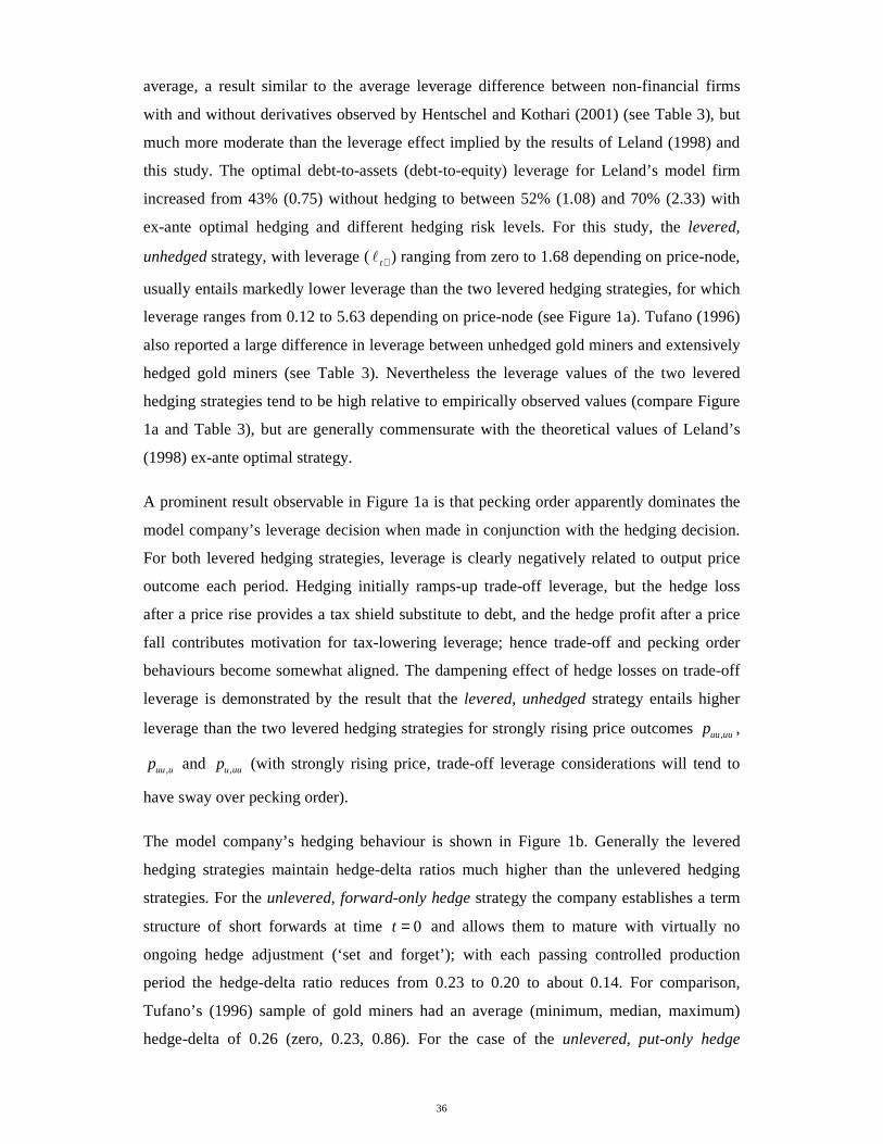
36

average, a result similar to the average leverage difference between non-financial firms

with and without derivatives observed by Hentschel and Kothari (2001) (see Table 3), but

much more moderate than the leverage effect implied by the results of Leland (1998) and

this study. The optimal debt-to-assets (debt-to-equity) leverage for Leland’s model firm

increased from 43% (0.75) without hedging to between 52% (1.08) and 70% (2.33) with

ex-ante optimal hedging and different hedging risk levels. For this study, the levered,

unhedged strategy, with leverage (t+l ) ranging from zero to 1.68 depending on price-node,

usually entails markedly lower leverage than the two levered hedging strategies, for which

leverage ranges from 0.12 to 5.63 depending on price-node (see Figure 1a). Tufano (1996)

also reported a large difference in leverage between unhedged gold miners and extensively

hedged gold miners (see Table 3). Nevertheless the leverage values of the two levered

hedging strategies tend to be high relative to empirically observed values (compare Figure

1a and Table 3), but are generally commensurate with the theoretical values of Leland’s

(1998) ex-ante optimal strategy.

A prominent result observable in Figure 1a is that pecking order apparently dominates the

model company’s leverage decision when made in conjunction with the hedging decision.

For both levered hedging strategies, leverage is clearly negatively related to output price

outcome each period. Hedging initially ramps-up trade-off leverage, but the hedge loss

after a price rise provides a tax shield substitute to debt, and the hedge profit after a price

fall contributes motivation for tax-lowering leverage; hence trade-off and pecking order

behaviours become somewhat aligned. The dampening effect of hedge losses on trade-off

leverage is demonstrated by the result that the levered, unhedged strategy entails higher

leverage than the two levered hedging strategies for strongly rising price outcomes ,uu uup ,

,uu up and ,u uup (with strongly rising price, trade-off leverage considerations will tend to

have sway over pecking order).

The model company’s hedging behaviour is shown in Figure 1b. Generally the levered

hedging strategies maintain hedge-delta ratios much higher than the unlevered hedging

strategies. For the unlevered, forward-only hedge strategy the company establishes a term

structure of short forwards at time 0t = and allows them to mature with virtually no

ongoing hedge adjustment (‘set and forget’); with each passing controlled production

period the hedge-delta ratio reduces from 0.23 to 0.20 to about 0.14. For comparison,

Tufano’s (1996) sample of gold miners had an average (minimum, median, maximum)

hedge-delta of 0.26 (zero, 0.23, 0.86). For the case of the unlevered, put-only hedge

37

strategy, an initial (time 0t = ) term structure of put options is occasionally followed up

with new put options; this and put option payoff non-linearity means that the hedge-delta

ratio is negatively related to price outcome each control period. For this strategy the hedge-

delta ratio varies between zero and 0.20 depending on price-node.

Table 3 – Empirical mean and median leverage values

Mean and median leverage values obtained by a variety of empirical studies.

Leverage (debt-to-equity basis)

Study Sample description Leverage measure Mean Median

Tufano (1996)

32 yearly observations from 1991 to 1993 of North Amer-ican gold mining firms with no net gold price hedging.

Tufano reported the ratio of {book value of debt} to {market value of equity plus book value of preferred stock and debt}.*

0.15

0.13

1 0.13=

−

0.05

0.05

1 0.05=

−

’’ 28 yearly observations from 1991 to 1993 of North Amer-ican gold mining firms with extensive net gold price hedg-ing.

’’ 0.22

0.18

1 0.18=

−

0.16

0.14

1 0.14=

−

Graham (1999)

65,429 yearly observations of COMPUSTAT firms from 1980 to 1994.

Graham reported the ratio of {long-term and current debt} to {book value of total assets minus book value of equity plus market value of equity}.*

0.27

0.213

1 0.213=

−

0.22

0.177

1 0.177=

−

Haushalter (2000)

295 yearly observations from 1992 to 1994 of oil and gas producing firms.

Haushalter reported the ratio of {long-term and current debt} to {market value of total assets}.*

0.29

0.226

1 0.226=

−

0.26

0.209

1 0.209=

−

Hentschel & Kothari (2001)

296 yearly observations from 1990 to 1993 of large US non-financial firms without deriv-ative positions.

Ratio of {book value of liabilities} to {market value of equity}.

1.68 1.08

’’ 394 yearly observations from 1990 to 1993 of large US non-financial firms with derivative positions.

’’ 1.75 1.09

Adam (2002)

595 yearly observations from 1989 to 1999 of North Amer-ican gold mining firms.

Ratio of {book value of long-term debt and preferred stock} to {book value of common equity}.

0.23 0.16

Flannery & Rangan (2006)

111,106 yearly observations of industrial COMPUSTAT firms from 1965 to 2001.

Flannery and Rangan reported the ratio of {book value of debt} to {book value of debt plus market value of common shares}.*

0.39

0.278

1 0.278=

−

0.29

0.225

1 0.225=

−

* The reported mean and median leverage values of these studies are here converted to a debt-to-equity ratio basis by dividing each value by its own complement relative to one.

38

For the cases of both levered hedging strategies, the model company establishes a term

structure of short forwards at time 0t = , but in response to a ‘weak’ output price outcome

( 1.01tp∆ = , 2 1.50tp ∆ ≤ ) the company actively reverses its overall hedge position in part or

in whole. This corresponds with evidence from Graham and Rogers (2002) who found that

firms reduce hedging in response to accumulated operating losses. In fact, if output price

falls to near the expected unit production cost at commencement of the third controlled

production period ( 2 1.01tp ∆ = ), the hedge position is switched to a speculatively long

stance. As such the hedge-delta ratios of the two levered hedging strategies vary from a

minimum of -0.11 up to 0.54 depending on price-node.

By model set-up, together with every control decision, debt-holders and other non-equity

stakeholders are fairly compensated for their limited liability risk. Hence the apparent asset

substitution decision to reduce hedging or switch to speculation does not manifest wealth

transfer from non-equity to equity. Instead it must be driven by cost/benefit asymmetry

between upside and downside output price outcomes. At outset (time 0t = ) the model

company’s jointly optimal hedging and leverage decision boosts the levels of both hedging

and leverage (compared to the company being optimally hedged and unlevered, and

optimally levered and unhedged respectively). Then as long as output price is generally

rising (from 0 1.50p = to 1.50tp∆ ≥ and 2 2.24tp ∆ ≥ ), the hedging level is largely

maintained, while leverage generally falls due to maturing-hedge losses substituting for

debt as a tax shield. For conversely weak price outcomes ( 1.01tp∆ = , 2 1.50tp ∆ ≤ ), the

company’s ongoing operational value is low, but the hedge portfolio is deep in-the-money

and facilitative of increased leverage driven by pecking order roll-over of hedging-boosted

debt plus tax-shielding of maturing-hedge profit. For the hedging decision, low ongoing

operational value imposes a net cost/benefit asymmetry with respect to output price

outcome, because an output price fall to below unit production cost will lead to

abandonment/bankruptcy regardless of hedge portfolio value, but an output price rise will

warrant continued operation and production.

Given a weak output price outcome and attendant deep in-the-money hedge portfolio, high

leverage and low ongoing operational value, the operational benefit of a subsequent output

price rise is vulnerable to the financial risk posed by the high leverage and the fact that the

hedge portfolio would lose value; that is, an output price rise actually entails adversely

high risk of bankruptcy and consequential foregone profitable production. To counter such

circumstance, reduced hedging or even a switch of the hedging decision to a speculatively

39

long stance increases the likelihood that the company will avoid bankruptcy in event of an

output price rise and thereby benefit from ongoing profitable production. Consequently the

facilitative relationship from hedging to leverage gets completely undone.

3.2. Base-case financial risk

At outset the two levered hedging strategies have, by all risk measures considered, equal or

lower risk than the other four control strategies (see Figures 1d to 1h at time 0t = ). But

this changes depending on output price behaviour and risk measure. The relative limited

liability risk measure ( /t tO E+ +− , see Figure 1d) indicates the proportion of equity value

( tE + ) attributable to the value of equity’s comprehensive limited liability option ( tO +− ).

The hedge reducing behaviour associated with the levered hedging strategies at weak price

outcomes ( 1.01tp∆ = , 2 1.50tp ∆ ≤ ), more strongly evident for the levered, forward+put

hedge strategy, exacerbates limited liability risk; sometimes this entails a value of

/t tO E+ +− greater than one, meaning that the limited liability option is in-the-money (i.e.

unlimited liability equity would have negative value). As long as output price is generally

rising (from 0 1.50p = to 1.50tp∆ ≥ and 2 2.24tp ∆ ≥ ), limited liability risk is very low or

zero for all control strategies.

Equity’s relative value-at-risk measure (tυ + , see Figure 1e) indicates the fraction of equity

value that will be lost with a ‘large-down’ price move (for which the risk-neutral

probability of occurrence is 0.0623). While output price is generally rising (from 0 1.50p =

to 1.50tp∆ ≥ to 2 2.24tp ∆ ≥ ), the levered hedging strategies have low or moderate value-

at-risk in comparison to the other control strategies. But for weak price outcomes

( 1.01tp∆ = , 2 1.50tp ∆ ≤ ) the levered, forward+put hedge strategy exhibits comparatively

high value-at-risk. However the levered, forward-only hedge strategy tends to keep value-

at-risk comparatively low or moderate even for weak price outcomes (especially at time

t t= ∆ ). The levered, unhedged strategy consistently has the highest or equal highest value-

at-risk.

Equity’s output price beta (tβ + , see Figure 1f) varies between 1.11 and 4.26 across all

output price outcomes and control strategies, and is clearly negatively related to output

price outcome. Nearly always the levered, unhedged strategy has the highest beta.

40

Generally the two levered hedging strategies have beta values lower than or similar to the

two unlevered hedging strategies, except when price is very weak ( 2 1.01tp ∆ = ); this is

associated with the fact that the levered hedging strategies generally have much higher

hedge-delta ratios than the unlevered hedging strategies, except when price is very weak.

These results are consistent with the empirical evidence of Tufano (1998), whose sample

of gold miners had a mean (first quartile, median, third quartile) three-monthly gold price

beta equal to 2.21 (1.13, 2.09, 3.13). Tufano found the miners’ gold price betas to be

negatively related to their extent of hedging, positively related to their financial leverage,

and negatively related to the gold price level.

The ex-post probability of bankruptcy measure (Pr tB − , see Figure 1g) indicates the

probability of bankruptcy at a price-node due to production quantity risk for the preceding

production period. For the first two controlled production periods, production quantity risk

predominantly poses negligible bankruptcy threat, though distinct exception applies for the

unlevered, unhedged and levered, unhedged strategies at low price outcome 1.01tp = .

Figure 1h shows that the risk-neutral ongoing (unconditional) probability of bankruptcy

( Pr tB + ) for the levered hedging strategies only becomes large in comparison to the other

control strategies for weak price outcomes commencing the third controlled production

period ( 2 1.50tp ∆ ≤ ). That is, although the levered hedging strategies demonstrate hedge

reduction for a weak price outcome commencing the second controlled production period

( 1.01tp∆ = ), the likelihood of the model company surviving into the third production

period is not disadvantaged relative to the other control strategies. This is particularly

notable for the levered, forward+put hedge strategy: at price-node dp , the levered,

forward+put hedge strategy markedly reduces total hedging leading to a large increase in

limited liability risk and value-at-risk, yet probability of bankruptcy for the ensuing period

stays subdued and on a par with the unlevered hedging strategies. For the case of the

levered, forward-only hedge strategy, total hedging is moderately reduced at price-node

dp , yet all risk measures remain comparatively low. These results for the levered hedging

strategies arise from the fact that, in response to a weak price outcome at time t t= ∆ , the

company uses its hedging term structure to both promote survival (since the company is

early in its production life), and to pre-empt a reduced hedging position if price weakness

persists at time 2t t= ∆ leading into the third and penultimate production period.

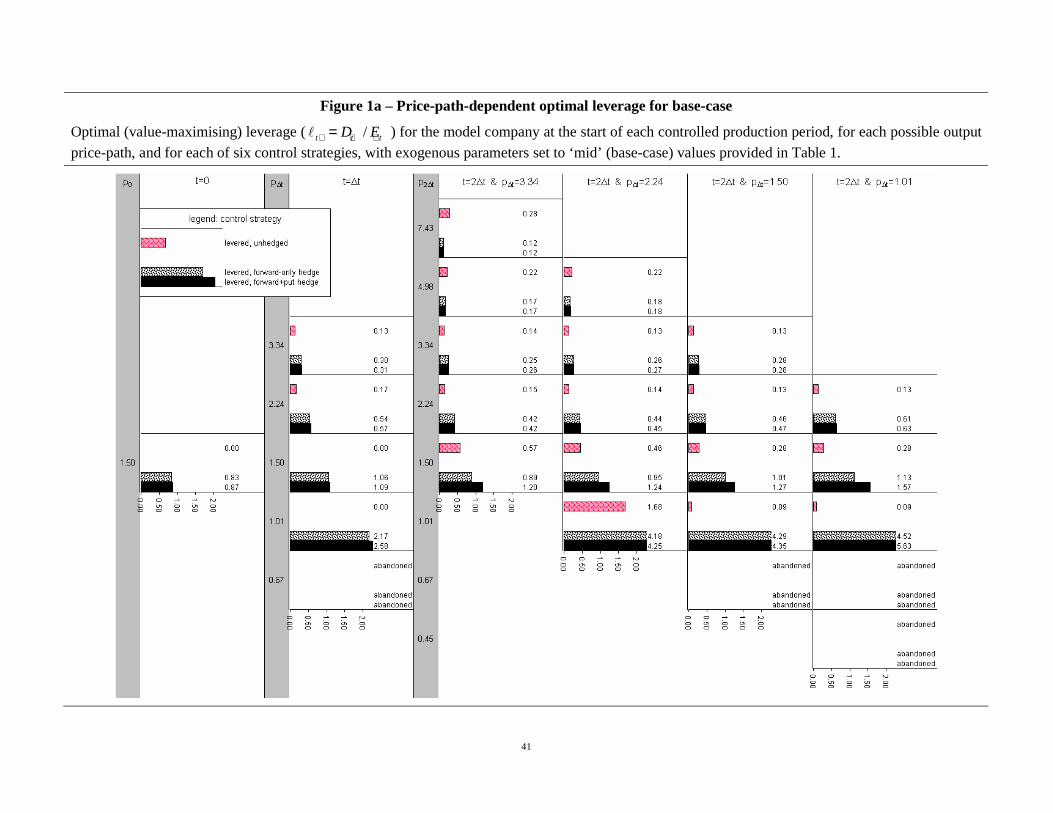
41

Figure 1a – Price-path-dependent optimal leverage for base-case

Optimal (value-maximising) leverage ( /t t tD E+ + +=l ) for the model company at the start of each controlled production period, for each possible output price-path, and for each of six control strategies, with exogenous parameters set to ‘mid’ (base-case) values provided in Table 1.

42

Figure 1b – Price-path-dependent optimal hedge-delta ratio for base-case

Optimal (value-maximising) hedge-delta ratio (th + ) for the model company at the start of each controlled production period, for each possible output price-path, and for each of six control strategies, with exogenous parameters set to ‘mid’ (base-case) values provided in Table 1.

43

Figure 1c – Price-path-dependent total company value (pre-control decisions) for base-case

Total value of the model company at the start of each controlled production period instantaneously before new control decisions are instigated

( ˆ [ ( ) | ]t t t t t tE D O p−∆ − − −Ε + + ), for each possible output price-path, and for each of six control strategies, with exogenous parameters set to ‘mid’ (base-case) values provided in Table 1.

44

Figure 1d – Price-path-dependent limited liability risk for base-case

Relative limited liability risk ( /t tO E+ +− ) for the value-maximised model company at the start of each controlled production period, for each possible output price-path, and for each of six control strategies, with exogenous parameters set to ‘mid’ (base-case) values provided in Table 1.

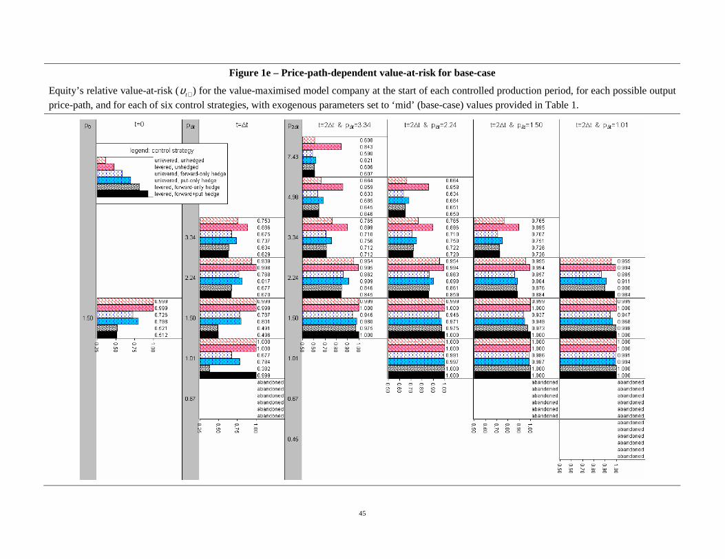
45

Figure 1e – Price-path-dependent value-at-risk for base-case

Equity’s relative value-at-risk (tυ + ) for the value-maximised model company at the start of each controlled production period, for each possible output price-path, and for each of six control strategies, with exogenous parameters set to ‘mid’ (base-case) values provided in Table 1.

46

Figure 1f – Price-path-dependent beta for base-case

Equity’s output price beta (tβ + ) for the value-maximised model company at the start of each controlled production period, for each possible output price-path, and for each of six control strategies, with exogenous parameters set to ‘mid’ (base-case) values provided in Table 1.

47

Figure 1g – Price-path-dependent ex-post probability of bankruptcy for base-case

Probability of bankruptcy for the preceding production period due to production quantity risk (Pr tB − ) for the value-maximised model company at the start of each controlled production period, for each possible output price-path, and for each of six control strategies, with exogenous parameters set to ‘mid’ (base-case) values provided in Table 1.

48

Figure 1h – Price-path-dependent ongoing probability of bankruptcy for base-case

Probability of bankruptcy for the ensuing production period (Pr tB + ) for the value-maximised model company at the start of each controlled production

period, for each possible output price-path, and for each of six control strategies, with exogenous parameters set to ‘mid’ (base-case) values provided in Table 1.

49

4. SENSITIVITY ANALYSIS

In progress. The aim is to determine whether the generalised/qualitative base-case results

persist when exogenous parameters are set ‘low’ or ‘top’ values.

5. CONCLUSION

To investigate both the value and risk impacts of a joint hedging and leverage decision, this

study utilises a multi-period model for a company subject to respectively hedgeable and

unhedgeable production output price and quantity risk variables, endogenously derived

deadweight costs, and the tandem availability of risky leverage and flexible hedging

control variables. It is found that an optimal (value-maximising) joint hedging and leverage

strategy can increase company value by about 3.4% compared to an unhedged optimal

leverage strategy, by about 2.2% compared to an unlevered optimal hedge strategy, and by

about 3.6% compared to the company being unlevered and unhedged. Also found is that

optimal leverage is usually much higher in conjunction with optimal hedging than with no

hedging, but the relationship is observed to not purely be a matter of higher hedging

facilitating higher leverage.

At outset a jointly optimal hedging and leverage strategy markedly boosts the levels of

both hedging and leverage, compared to optimal hedging without leverage, and optimal

leverage without hedging respectively. Then as long as the price for production output is at

least rising modestly, the hedging level is largely maintained, while leverage tends to fall

due to maturing-hedge losses substituting for debt as a tax shield. For conversely weak

output price outcomes close to the unit cost of production, the ongoing operational value of

the company is low, particularly if the company is at a late stage of its production life, but

the hedge portfolio is deep in-the-money and facilitative of increased leverage driven by

pecking order roll-over of hedging-boosted debt plus tax-shielding of maturing-hedge

profit. For the hedging decision, low ongoing operational value imposes a net cost/benefit

asymmetry with respect to output price outcome, because an output price fall (below unit

production cost) will lead to abandonment/bankruptcy regardless of hedge portfolio value,

but an output price rise will warrant continued operation and production. Given a weak

price outcome and attendant deep in-the-money hedge portfolio, high leverage and low

ongoing operational value, the operational benefit of a subsequent output price rise is

50

vulnerable to the financial risk posed by the high leverage and the fact that the hedge

portfolio would lose value; that is, an output price rise actually entails adversely high risk

of bankruptcy and consequential foregone profitable production. To counter such

circumstance, reduced hedging or even a switch of the hedging decision to a speculatively

long stance increases the likelihood that the company will avoid bankruptcy in event of an

output price rise and thereby benefit from ongoing profitable production. The value-

maximising optimality of this risk-seeking behaviour arises in conjunction with fair

compensation to debt-holders and other non-equity stakeholders for limited liability risk.

Measures of financial risk consequently demonstrate that, for weak output price outcomes

close to the unit cost of production, an optimal joint hedging and leverage strategy is often

more risky than any of an unhedged optimal leverage strategy, an unlevered optimal hedge

strategy, or an unhedged and unlevered strategy; but the opposite is often evident at higher

price levels. Nevertheless, overall distinction of the relative financial riskiness of optimal

joint hedging and leverage versus alternative strategies is not easily generalised and shows

dependence not only on the output price level, but also on the company’s remaining

production life and the available hedging instruments.

51

APPENDIX A. THE MODEL

The intention is to define the model company’s equity and non-equity19 stakes as complex,

interdependent, American-style options on production and hedging cash-flows. Thereby an

option-pricing approach can be used to value equity and non-equity and to also assess the

effects of hedging and leverage control decisions. The model company faces two sources

of uncertainty: at time t , being the end of a discrete production period of duration t∆

years, the production output for the period is an uncertain quantity of tq units, and the

price obtainable for the production output is an uncertain amount of tp dollars per unit.

The bivariate price and quantity process is assumed to be Markovian. Hedging can only be

contracted with respect to price uncertainty (i.e. the price risk is hedgeable and the quantity

risk is unhedgeable). The company is assumed to have uniform production periods, and

periodic expected production quantity is assumed to be independent of previous

unexpected production quantity deviations. This allows the company to be specified as

blind to the history of the stochastic component of production quantities, which

advantageously allows equity and non-equity, conditional on price and control variables, to

have generalisable valuation solutions with respect to quantity uncertainty.

Price and quantity random variable specification

Assume that the production output price and quantity are lognormal random variables such

that their risk-neutral processes are:

2

( )

( )2

00

ln2ln

lnln ln ( )

2

pt t p

p tt

qt q tq pt t

p

p r ttp

q tpq r t t

p

σδ

σ ψ

σ ψσ σρ δ

σ

−∆

−∆

+ − − ∆ ∆

= + ∆ + − − − − ∆

,

( )

( )

0 1~ N ,

0 1

pt

qt

ρψρψ

19 The non-equity stake refers to the combined position of debt plus the short comprehensive limited liability

option provided to equity by all non-equity stakeholders in the company.

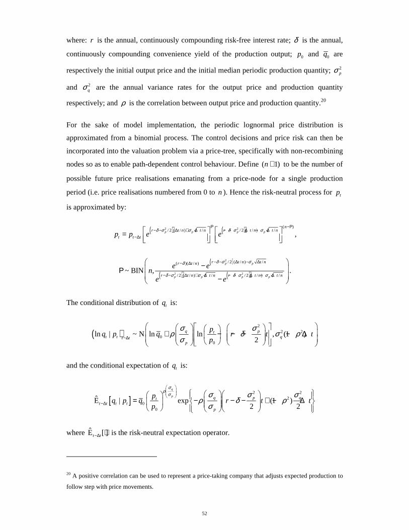
52

where: r is the annual, continuously compounding risk-free interest rate; δ is the annual,

continuously compounding convenience yield of the production output; 0p and 0q are

respectively the initial output price and the initial median periodic production quantity; 2pσ

and 2qσ are the annual variance rates for the output price and production quantity

respectively; and ρ is the correlation between output price and production quantity.20

For the sake of model implementation, the periodic lognormal price distribution is

approximated from a binomial process. The control decisions and price risk can then be

incorporated into the valuation problem via a price-tree, specifically with non-recombining

nodes so as to enable path-dependent control behaviour. Define ( 1)n + to be the number of

possible future price realisations emanating from a price-node for a single production

period (i.e. price realisations numbered from 0 to n ). Hence the risk-neutral process for tp

is approximated by:

( ) ( )2 2 ( )/ 2 ( / ) / / 2 ( / ) /p p p p

nr t n t n r t n t n

t t tp p e eδ σ σ δ σ σ

Ρ −Ρ− − ∆ + ∆ − − ∆ − ∆

−∆ =

,

( )

( ) ( )

2

2 2

/ 2 ( / ) /( )( / )

/ 2 ( / ) / / 2 ( / ) /~ BIN ,

p p

p p p p

r t n t nr t n

r t n t n r t n t n

e en

e e

δ σ σδ

δ σ σ δ σ σ

− − ∆ − ∆− ∆

− − ∆ + ∆ − − ∆ − ∆

− Ρ −

.

The conditional distribution of tq is:

( )2

2 20

0

ln | ~ N ln ln , (1 )2

q ptt t qt t

p

pq p q r t t

p

σ σρ δ σ ρ

σ−∆

+ − − − − ∆

and the conditional expectation of tq is:

[ ]2 2

20

0

E | exp (1 )2 2

q

p q p qtt t t t

p

pq p q r t t

p

σρ

σ σ σ σρ δ ρ

σ

−∆

= − − − + − ∆

where E [ ]t t−∆ ⋅ is the risk-neutral expectation operator.

20 A positive correlation can be used to represent a price-taking company that adjusts expected production to

follow step with price movements.

53

Furthermore, for later reference, the risk-neutral conditional expected payoffs for a vanilla

put option, an asset-or-nothing digital put option and a cash-or-nothing digital put option

contracted on tq with strike χ (respectively designated as VPtq χ< , ADP

tq χ< and CDPtq χ< )

are:

[ ]( )

[ ] [ ] ( )( )

2 2

2 2

ˆVP E ( ) I |

ˆˆ ln E ln | 1ln E ln |E | ,

1 1

t tq t t t q t

t t t t qt t t tt t t t

q q

q p

q p tq pq p

t t

χ χχ

χ σ ρχχ

σ ρ σ ρ

< −∆ <

−∆−∆−∆

= −

− − − ∆− = Φ − Φ − ∆ − ∆

[ ] [ ] ( )( )

2 2

2

ˆln E ln | 1ˆ ˆADP E I | E | ,

1t t

t t t t q

q t t t q t t t t t

q

q p tq p q p

tχ χ

χ σ ρ

σ ρ−∆

< −∆ < −∆

− − − ∆ = = Φ − ∆

[ ]( )2

ˆln E ln |ˆCDP E I |1

t t

t t t tq t t q t

q

q pp

tχ χ

χ

σ ρ−∆

< −∆ <

− = = Φ − ∆

where: the indicator function, I logical statement , equals one if the logical statement is true and

zero otherwise; and {}Φ ⋅ is the standard normal cumulative distribution function.

Control variables

Define positive integer N to be the number of production periods for which control

decisions will be made: N may cover the company’s total production life or, if an estimate

can be made for ongoing company value at some intermediate stage of its total life, N

may then be the number of production periods up to this intermediate stage. Time is

denominated by the discrete production periods { }( )0, ,2 ,...,t t t N t∈ ∆ ∆ ∆ . Given the

positive integer approximation of ( 1)n + possible price realisations for a production

period, the total number of non-recombining price-paths is therefore equal to ( 1)Nn + .

Define { }1,2,..., ( 1)Nnη ∈ + to signify a specific price-path.

The company has control over hedging and leverage. The hedging control decision at each

start-of-period entails application of a hedging term structure comprising a series of hedge

quantities ( ,t t tx κ+ ∆ production units) for hedge contracts with initial terms to maturity ( tκ∆ )

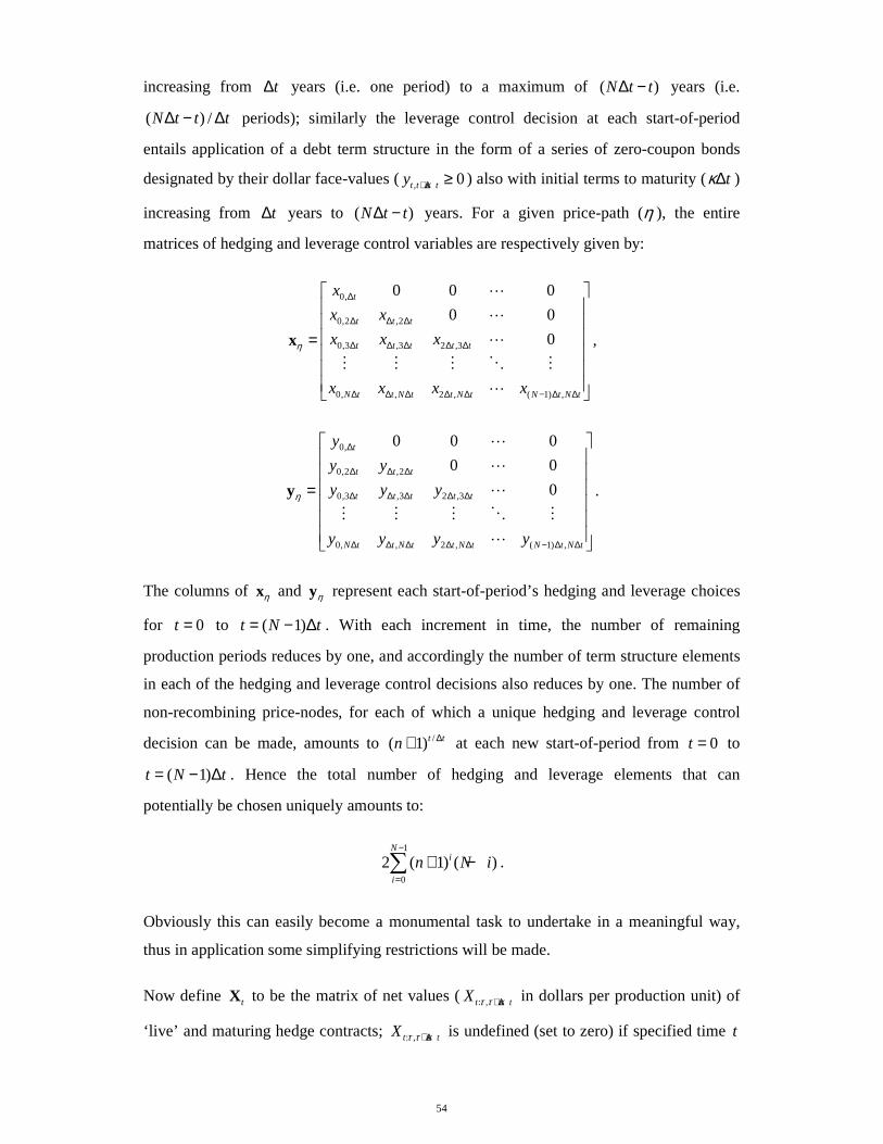
54

increasing from t∆ years (i.e. one period) to a maximum of ( )N t t∆ − years (i.e.

( ) /N t t t∆ − ∆ periods); similarly the leverage control decision at each start-of-period

entails application of a debt term structure in the form of a series of zero-coupon bonds

designated by their dollar face-values (, 0t t ty κ+ ∆ ≥ ) also with initial terms to maturity ( tκ∆ )

increasing from t∆ years to ( )N t t∆ − years. For a given price-path (η ), the entire

matrices of hedging and leverage control variables are respectively given by:

0,

0,2 ,2

0,3 ,3 2 ,3

0, , 2 , ( 1) ,

0 0 0

0 0

0

t

t t t

t t t t t

N t t N t t N t N t N t

x

x x

x x x

x x x x

η

∆

∆ ∆ ∆

∆ ∆ ∆ ∆ ∆

∆ ∆ ∆ ∆ ∆ − ∆ ∆

=

x

L

L

L

M M M O M

L

,

0,

0,2 ,2

0,3 ,3 2 ,3

0, , 2 , ( 1) ,

0 0 0

0 0

0

t

t t t

t t t t t

N t t N t t N t N t N t

y

y y

y y y

y y y y

η

∆

∆ ∆ ∆

∆ ∆ ∆ ∆ ∆

∆ ∆ ∆ ∆ ∆ − ∆ ∆

=

y

L

L

L

M M M O M

L

.

The columns of ηx and ηy represent each start-of-period’s hedging and leverage choices

for 0t = to ( 1)t N t= − ∆ . With each increment in time, the number of remaining

production periods reduces by one, and accordingly the number of term structure elements

in each of the hedging and leverage control decisions also reduces by one. The number of

non-recombining price-nodes, for each of which a unique hedging and leverage control

decision can be made, amounts to /( 1)t tn ∆+ at each new start-of-period from 0t = to

( 1)t N t= − ∆ . Hence the total number of hedging and leverage elements that can

potentially be chosen uniquely amounts to:

1

0

2 ( 1) ( )N

i

i

n N i−

=+ −∑ .

Obviously this can easily become a monumental task to undertake in a meaningful way,

thus in application some simplifying restrictions will be made.

Now define tX to be the matrix of net values (: ,t tX τ τ κ+ ∆ in dollars per production unit) of

‘live’ and maturing hedge contracts; : ,t tX τ τ κ+ ∆ is undefined (set to zero) if specified time t

55

is earlier than hedge contract initiation at time τ or later than hedge contract maturity at

time ( )tτ κ+ ∆ (i.e. : , 0t tX τ τ κ+ ∆ = if t τ< or ( )t tτ κ> + ∆ ):

:0,

:0,2 : ,2

:0,3 : ,3 :2 ,3

:0, : , :2 , :( 1) ,

0 0 0

0 0

0

t t

t t t t t

t t t t t t t tt

t N t t t N t t t N t t N t N t

X

X X

X X X

X X X X

∆

∆ ∆ ∆

∆ ∆ ∆ ∆ ∆

∆ ∆ ∆ ∆ ∆ − ∆ ∆

=

X

L

L

L

M M M O M

L

.

The hedge contracts are assumed to have zero upfront cost (i.e. the applicable upfront

hedge contract premium, if any, is compounded forward at the risk-free interest rate and

included as a negative amount in the net hedge payoff calculation at contract maturity).

Hence the net value of each hedge contract at initiation ( : ,t t t tX κ+ ∆ ) is set to zero. If the

hedge contracts mature in favour of the company (: , 0t t t tX κ− ∆ > ), they contribute to end-of-

period revenue. If the hedge contracts mature out of the company’s favour ( : , 0t t t tX κ− ∆ < ),

they become an end-of-period liability.

Hedge specification

The model company is assumed able to combine a short forward hedge with a put option

hedge. In addition to control of hedge quantity (described by matrix ηx ), at each start-of-

period the company can also choose a term structure for: the fraction of total hedge

quantity committed to short forwards as opposed to put options ( ,0 1t t tw κ+ ∆≤ ≤ , i.e.

, ,t t t t t tw xκ κ+ ∆ + ∆ production units are hedged with short forwards and , ,(1 )t t t t t tw xκ κ+ ∆ + ∆− units

are hedged with put options); and the strike price of the put options ( , 0t t tz κ+ ∆ > ). The entire

matrices of these additional hedging control variables are:

0,

0,2 ,2

0,3 ,3 2 ,3

0, , 2 , ( 1) ,

0 0 0

0 0

0

t

t t t

t t t t t

N t t N t t N t N t N t

w

w w

w w w

w w w w

η

∆

∆ ∆ ∆

∆ ∆ ∆ ∆ ∆

∆ ∆ ∆ ∆ ∆ − ∆ ∆

=

w

L

L

L

M M M O M

L

,

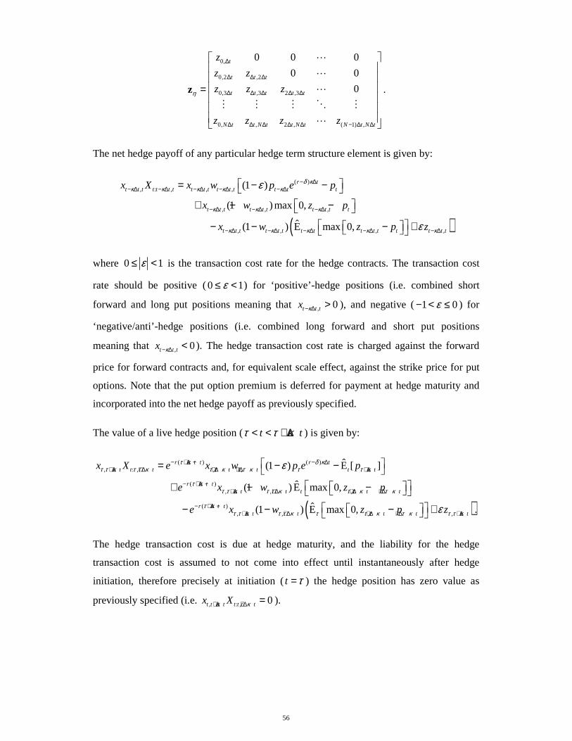
56

0,

0,2 ,2

0,3 ,3 2 ,3

0, , 2 , ( 1) ,

0 0 0

0 0

0

t

t t t

t t t t t

N t t N t t N t N t N t

z

z z

z z z

z z z z

η

∆

∆ ∆ ∆

∆ ∆ ∆ ∆ ∆

∆ ∆ ∆ ∆ ∆ − ∆ ∆

=

z

L

L

L

M M M O M

L

.

The net hedge payoff of any particular hedge term structure element is given by:

( )

( ), : , , ,

, , ,

, , , ,

(1 )

(1 )max 0,

ˆ(1 ) E max 0,

r tt t t t t t t t t t t t t t t t

t t t t t t t t t t

t t t t t t t t t t t t t t t

x X x w p e p

x w z p

x w z p z

δ κκ κ κ κ κ

κ κ κ

κ κ κ κ κ

ε

ε

− ∆− ∆ − ∆ − ∆ − ∆ − ∆

− ∆ − ∆ − ∆

− ∆ − ∆ − ∆ − ∆ − ∆

= − −

+ − −

− − − +

where 0 1ε≤ < is the transaction cost rate for the hedge contracts. The transaction cost

rate should be positive (0 1ε≤ < ) for ‘positive’-hedge positions (i.e. combined short

forward and long put positions meaning that , 0t t tx κ− ∆ > ), and negative (1 0ε− < ≤ ) for

‘negative/anti’-hedge positions (i.e. combined long forward and short put positions

meaning that , 0t t tx κ− ∆ < ). The hedge transaction cost rate is charged against the forward

price for forward contracts and, for equivalent scale effect, against the strike price for put

options. Note that the put option premium is deferred for payment at hedge maturity and

incorporated into the net hedge payoff as previously specified.

The value of a live hedge position ( t tτ τ κ< < + ∆ ) is given by:

( ) ( ), : , , ,

( ), , ,

( ), , ,

ˆ(1 ) E [ ]

ˆ(1 )E max 0,

ˆ(1 ) E max 0,

r t t r tt t t t t t t

r t tt t t t t

r t tt t t t

x X e x w p e p

e x w z p

e x w z p

τ κ δ κτ τ κ τ τ κ τ τ κ τ τ κ τ τ κ

τ κτ τ κ τ τ κ τ τ κ τ κ

τ κτ τ κ τ τ κ τ τ τ κ τ κ

ε− + ∆ − − ∆+ ∆ + ∆ + ∆ + ∆ + ∆

− + ∆ −+ ∆ + ∆ + ∆ + ∆

− + ∆ −+ ∆ + ∆ + ∆ + ∆

= − −

+ − −

− − −( ), .tzτ τ κε + ∆ +

The hedge transaction cost is due at hedge maturity, and the liability for the hedge

transaction cost is assumed to not come into effect until instantaneously after hedge

initiation, therefore precisely at initiation (t τ= ) the hedge position has zero value as

previously specified (i.e. , : , 0t t t t t t tx Xκ κ+ ∆ + ∆ = ).

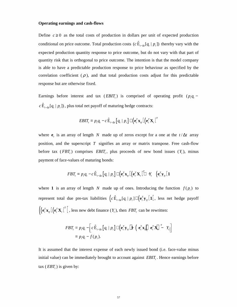
57

Operating earnings and cash-flows

Define 0c ≥ as the total costs of production in dollars per unit of expected production

conditional on price outcome. Total production costs ˆ( E [ | ])t t t tc q p−∆ thereby vary with the

expected production quantity response to price outcome, but do not vary with that part of

quantity risk that is orthogonal to price outcome. The intention is that the model company

is able to have a predictable production response to price behaviour as specified by the

correlation coefficient (ρ ), and that total production costs adjust for this predictable

response but are otherwise fixed.

Earnings before interest and tax ( tEBIT ) is comprised of operating profit ( t tp q −

E [ | ])t t t tc q p−∆ , plus total net payoff of maturing hedge contracts:

[ ] ( )( )E |TT T

t t t t t t t t t tEBIT p q c q p η−∆= − + e x e X

where te is an array of length N made up of zeros except for a one at the /t t∆ array

position, and the superscript T signifies an array or matrix transpose. Free cash-flow

before tax ( tFBT ) comprises tEBIT , plus proceeds of new bond issues (tY ), minus

payment of face-values of maturing bonds:

[ ] ( )( ) ( )E |TT T T

t t t t t t t t t t t tFBT p q c q p Yη η−∆= − + + −e x e X e y 1

where 1 is an array of length N made up of ones. Introducing the function ( )tf p to

represent total due pre-tax liabilities ( )( )E [ | ] Tt t t t tc q p η−∆ + e y 1 , less net hedge payoff

( )( )( )TT Tt t tηe x e X , less new debt finance (tY ), then tFBT can be rewritten:

[ ] ( ) ( )( )E |

( ).

TT T Tt t t t t t t t t t t t

t t t

FBT p q c q p Y

p q f p

η η−∆ = − + − −

= −

e y 1 e x e X

It is assumed that the interest expense of each newly issued bond (i.e. face-value minus

initial value) can be immediately brought to account against tEBIT . Hence earnings before

tax ( tEBT ) is given by:

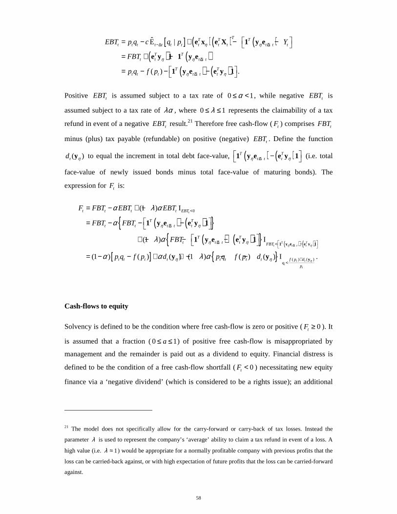
58

[ ] ( )( ) ( )( ) ( )

( ) ( )

E |

( ) .

TT T Tt t t t t t t t t t t t t

T Tt t t t

T Tt t t t t t

EBT p q c q p Y

FBT

p q f p

η η

η η

η η

−∆ +∆

+∆

+∆

= − + − −

= + −

= − − −

e x e X 1 y e

e y 1 1 y e

1 y e e y 1

Positive tEBT is assumed subject to a tax rate of 0 1α≤ < , while negative tEBT is

assumed subject to a tax rate of λα , where 0 1λ≤ ≤ represents the claimability of a tax

refund in event of a negative tEBT result.21 Therefore free cash-flow (tF ) comprises tFBT

minus (plus) tax payable (refundable) on positive (negative) tEBT . Define the function

( )td ηy to equal the increment in total debt face-value, ( ) ( )T Tt t tη η+∆

− 1 y e e y 1 (i.e. total

face-value of newly issued bonds minus total face-value of maturing bonds). The

expression for tF is:

( ) ( ){ }( ) ( ){ } ( ) ( )

[ ] { }

0

( ) ( )

(1 ) I

(1 ) I

(1 ) ( ) ( ) (1 ) ( ) ( ) I .

t

T Tt t t t

t tt

t

t t t t EBT

T Tt t t t t

T Tt t t t FBT

t t t t t t t t f p dq

p

F FBT EBT EBT

FBT FBT

FBT

p q f p d p q f p d

η η

η

η η

η η

η η

α λ α

α

λ α

α α λ α+∆

<

+∆

+∆ < −

+<

= − + −

= − − −

+ − − −

= − − + + − − −

1 y e e y 1

y

1 y e e y 1

1 y e e y 1

y y

Cash-flows to equity

Solvency is defined to be the condition where free cash-flow is zero or positive ( 0tF ≥ ). It

is assumed that a fraction (0 1a≤ ≤ ) of positive free cash-flow is misappropriated by

management and the remainder is paid out as a dividend to equity. Financial distress is

defined to be the condition of a free cash-flow shortfall ( 0tF < ) necessitating new equity

finance via a ‘negative dividend’ (which is considered to be a rights issue); an additional

21 The model does not specifically allow for the carry-forward or carry-back of tax losses. Instead the

parameter λ is used to represent the company’s ‘average’ ability to claim a tax refund in event of a loss. A

high value (i.e. 1λ ≈ ) would be appropriate for a normally profitable company with previous profits that the

loss can be carried-back against, or with high expectation of future profits that the loss can be carried-forward

against.

59

fraction ( 0γ ≥ ) of the free cash-flow shortfall is required from equity finance providers to

cover financial distress costs and the transaction costs of the equity issue. Bankruptcy is

defined to occur under condition of negative free cash-flow such that the required equity-

raising ( (1 ) tFγ− + ) is larger than the ongoing equity value (being the present value of

future cash-flows to equity given that bankruptcy has not occurred). Using 0tE + ≥ to

signify the ongoing equity value, the dividend payment ( tG ) is determined as follows:

0

(1 )

(1 ) , 0

(1 ) , /(1 ) 0

0 , /(1 )

(1 ) ( ) I (1 ) I .t t

t

t t

t t t t

t t

t t F t EF

a F F

G F E F

F E

a F a F Fγ

γ γγ

γ γ+

+

+

< −<+

− ≥ = + − + ≤ < < − +

= − + + − +

Noting, for some value J , that:

(1 ) ( ) ( )

(1 )

(1 ) ( ) ( ) ( ) ( ) (1 ) ( ) ( ) ( ) ( )min , min ,

(1 ) (1 )

I I

I I .

t t tt

t

t t t t t t t tt t

t t t t

F J f p J dq

p

f p J d f p d f p J d f p dq q

p p p p

η

η η η η

α αα

α α αλ αλα αλ

< − + −<

−

− + − + − + − + < < − −

=

− +

y

y y y y

Then substituting for tF in the expression for tG gives:

[ ]

( ) ( )

(1 ) ( ) ( )

(1 )

(1 )(1 ) ( ) (1 ) ( )

( ) ( )(1 )(1 ) I

(1 ) ( ) ( )( )(1 ) I

(1 )

(1 ) ( ) ( )(1 )(1 )

(1

t tt

t

t tt

t

t t t t t

t tt t f p d

qt p

t tt t f p d

qt p

t tt

G a p q f p a d

f p da p q

p

f p da p q

p

f p dp

η

η

η

η

ηα α

α

η

α α

λ α

α αγ α

α

α αγ α

+<

− −<

−

= − − − + −

+ − − − −

− − − + − − −

− −+ + −

y

y

y

y

y

y(1 )(1 ) ( ) (1 ) ( )

(1 )(1 )

(1 ) ( ) ( ) ( ) ( )min ,

(1 )

I)

(1 ) ( ) ( )( )(1 ) I

(1 )

(1 ) ( ) ( )(1 )(1 )

(1 )

t t tt

t

t t t tt

t t

t f p E dq

t p

t tt t f p d f p d

qt p p

t tt

t

qp

f p da p q

p

f p dp

p

η

η η

γ α α γγ α

ηα α

α

η

α

α αγ α

α

α αγ α

α

++ − − − +<

+ −

− − + < −

− −

− − + + − − −

− −− + −

−

y

y y

y

y(1 )(1 ) ( ) (1 ) ( ) ( ) ( )

min ,(1 )(1 )

(1 ) ( ) ( ) ( ) ( )min ,

(1 )

I

(1 ) ( ) ( )( )(1 ) I

(1 )

(1 )(1 )

t t t t tt

t t

t t t tt

t t

t f p E d f p dq

p p

t tt t f p d f p d

qt p p

q

f p da p q

p

η η

η η

γ α α γγ α

ηαλ αλ

αλ

αλ αλγ αλ

αλ

γ αλ

++ − − − + + < + −

− − + < −

−

−

− − − + − − −

+ +

y y

y y

y

(1 )(1 ) ( ) (1 ) ( ) ( ) ( )min ,

(1 )(1 )

(1 ) ( ) ( )I

(1 ) t t t t tt

t t

t tt t f p E d f p d

qt p p

f p dp q

p η η

ηγ αλ αλ γ

γ αλ

αλ αλαλ +− − −+ + +

< + −

− −−

−

y y

y

60

Note that ( )tf p , ( )td ηy and tE + are dependent on tp but not tq (although tq does have a

role in determining whether bankruptcy occurs and thus whether tE + is accessed or not).

This means that at each period the expected dividend payment can be solved conditional on

tp . To do so it can be seen that the dividend payment comprises a series of put option

payoffs dependent on tq : two standard/vanilla put options; five asset-or-nothing digital put

options; and five cash-or-nothing digital put options. Recall that VPtq χ< , ADP

tq χ< and

CDPtq χ< signify the risk-neutral conditional expected payoffs respectively for a vanilla put

option, an asset-or-nothing digital put option and a cash-or-nothing digital put option

contracted on tq with strike χ . To simplify notation, define 1χ , 2χ , 3χ , 4χ and 5χ :

1

( ) ( )t t

t

f p d

pηχ

+=

y, 2

(1 ) ( ) ( )

(1 )t t

t

f p d

pηα α

χα

− −=

−y

,

3

(1 )(1 ) ( ) ( | ) (1 ) ( )

(1 )(1 )t t t t

t

f p E p d

pηγ α α γ

χγ α

++ − − − +=

+ −y

, 4

(1 ) ( ) ( )

(1 )t t

t

f p d

pηαλ αλ

χαλ

− −=

−y

,

5

(1 )(1 ) ( ) ( | ) (1 ) ( )

(1 )(1 )t t t t

t

f p E p d

pηγ αλ αλ γ

χγ αλ

++ − − − +=

+ −y

.

Hence:

[ ] [ ]{ }[ ] [ ]{ }

1 2 2 1 2 1

4 1 4 1

2 min , min ,

4 min , min ,

2

ˆ ˆE [ | ] (1 )(1 ) E [ | ] ( ) (1 ) ( )

(1 )(1 ) VP ( )(1 ) VP CDP ADP

( )(1 ) CDP ADP

(1 )(1 ) CDP

t t t t

t t

t

t t t t t t t t t t t

t q t q q q

t q q

t q

G p a p q p f p a d

a p a p

a p

p

η

χ χ χ χ χ χ

χ χ χ χ

α α

λ α γ α χ

γ αλ χ

γ α χ

−∆ −∆

< < < <

< <

= − − − + −

− − − − + − − +

− + − −

+ + −

y

[ ] [ ]{ }[ ] [ ]{ }

3 3 3 1 3 1

5 1 5 1

2 min , min ,

4 min , min ,

ADP CDP ADP

(1 )(1 ) CDP ADP .

t t t

t t

q q q

t q qp

χ χ χ χ χ χ

χ χ χ χ

χ

γ αλ χ

< < < <

< <

− − +

+ + − −

In the event of bankruptcy ( /(1 )t tF E γ+< − + ), the company is liquidated for a cash-flow

( tL ) equal to tEBIT plus the market value of the company’s live (non-maturing) hedge

contracts, minus the total face-value of outstanding debt (excluding new debt, which would

not be issued in event of bankruptcy) increased by a bankruptcy cost factor (b ):

[ ] ( ) ( )/

E | tr (1 )N

T Tt t t t t t t t i t t

i t t

L p q c q p bη η−∆ ∆= ∆

= − + − + ∑x X e y k

61

where tk is an array of length N made up of ones for the first array position through to

the /t t∆ array position and zeros otherwise. Introducing the function ( )tg p to represent

the company’s liquidation liability for production costs ( )E [ | ]t t t tc q p−∆ and for debt

( )( )/(1 )

N Ti t ti t t

b η∆= ∆+ ∑ e y k , less both the net hedge payoff of maturing contracts and the

market value of live hedge contracts ( )( )tr Ttηx X , then the liquidation cash-flow term can

be rewritten:

[ ] ( ) ( )/

E | (1 ) tr

( ).

NT T

t t t t t t t i t t ti t t

t t t

L p q c q p b

p q g p

η η−∆ ∆= ∆

= − + + −

= −

∑ e y k x X

The distribution of tL to non-equity stakeholders is capped at the total face-value of

outstanding debt. Any remainder is paid to equity as a taxable liquidating dividend ( tGL ):

{ } ( )

(1 )

(1 ) , 0 /(1 )(1 ) ( ) 1 I I .

0 , t tt t

t

t t t tt t t t g p E

q Fp

L L F EGL p q g p

otherwise γ

α γα

+

+−

< <+

− ≥ < − + = = − − −

I

Therefore:

[ ] [ ]{ }[ ] [ ]{ }

3 3 1 5 1

3 3 1 5 1

3 3 1 5 1

min , min ,

min , min ,

( ) ( ) ( )min , min , , min , ,

E [ | ] (1 ) ADP ADP ADP

(1 ) ( ) CDP CDP CDP

(1 ) ADP ADP ADP

t t t

t t t

t t tt t t

t t t

t t t t t q q q

t q q q

t g p g p g pq q q

p p p

GL p p

g p

p

χ χ χ χ χ

χ χ χ χ χ

χ χ χ χ χ

α

α

α

−∆ < < <

< < <

< < <

= − − +

− − − +

− − − +

3 3 1 5 1( ) ( ) ( )

min , min , , min , ,(1 ) ( ) CDP CDP CDP .

t t tt t t

t t t

t g p g p g pq q q

p p p

g pχ χ χ χ χ

α

< < <

+ − − +

The total value attributable to equity immediately prior to any dividend payment at time t

( tE − ) is given by:

(1 )

1 It

tt t t t E

FE G GL E

γ+− + −

<+

= + + −

.

Therefore:

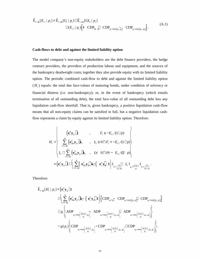
62

[ ] [ ]{ }3 3 1 5 1min , min ,

ˆ ˆ ˆE [ | ] E [ | ] E [ | ]

( | ) 1 CDP CDP CDP .t t t

t t t t t t t t t t t t

t t q q q

E p G p GL p

E p χ χ χ χ χ

−∆ − −∆ −∆

+ < < <

= +

+ − + − (A.1)

Cash-flows to debt and against the limited liability option

The model company’s non-equity stakeholders are the debt finance providers, the hedge

contract providers, the providers of production labour and equipment, and the sources of

the bankruptcy deadweight costs; together they also provide equity with its limited liability

option. The periodic combined cash-flow to debt and against the limited liability option

( tH ) equals: the total due face-values of maturing bonds, under condition of solvency or

financial distress (i.e. non-bankruptcy); or, in the event of bankruptcy (which entails

termination of all outstanding debt), the total face-value of all outstanding debt less any

liquidation cash-flow shortfall. That is, given bankruptcy, a positive liquidation cash-flow

means that all non-equity claims can be satisfied in full, but a negative liquidation cash-

flow represents a claim by equity against its limited liability option. Therefore:

( )( )

( )

( ) ( ) ( )

/

/

( )/ (1 ) (1 )

, /(1 )

, 0 /(1 )

, 0 /(1 )

I I I .t t t

t t tt

Tt t t

NT

t i t t t t ti t t

NT

t i t t t t ti t t

NT T Tt i t t t E t g p E

F q Fi t t p

F E

H L F E

L L F E

L

η

η

η

η η ηγ γ

γ

γ

γ

+ +

+

∆ += ∆

∆ += ∆

∆ − −< < <= ∆ + +

≥ − + = ≥ < − +

+ < < − +

= + − +

∑

∑

∑

e y 1

e y k

e y k

e y 1 e y k e y 1

I

I

Therefore:

( )( ) ( ) [ ] [ ]{ }3 3 1 5 1

3 3 1 5 1

min , min ,/

( ) ( ) ( )min , min , , min , ,

min

E [ | ]

CDP CDP CDP

ADP ADP ADP

( ) CDP

t t t

t t tt t t

t t t

t

Tt t t t t

NT Ti t t t q q q

i t t

t g p g p g pq q q

p p p

tq

H p

p

g p

η

η η χ χ χ χ χ

χ χ χ χ χ

−∆

∆ < < <= ∆

< < <

<

=

+ − − +

+ − +

−

∑

e y 1

e y k e y 1

3 3 1 5 1( ) ( ) ( )

, min , , min , ,CDP CDP .

t t tt t

t t t

g p g p g pq q

p p pχ χ χ χ χ

< <

− +

63

Consider that risky debt is a combination of risk-free debt plus a short position in a limited

liability option that has some individualised exercise priority amongst all the various

limited liability options provided by non-equity stakeholders to equity. This model is not

concerned with separating out the specific limited liability exposure of debt from other

non-equity stakes. Instead the value of equity’s comprehensive limited liability option

underwritten by all of the non-equity stakes is of interest. To obtain this value it is

necessary to separate out the risk-free debt valuation from the total value of debt and the

short limited liability option. Thus define tD − , tD and tD + to each be the risk-free value of

all outstanding bonds at time t but respectively at the immediate instances: before

settlement of maturing bonds and before issue of any new bonds; after settlement of

maturing bonds and before issue of any new bonds; and after settlement of maturing bonds

and after issue of any new bonds. Therefore:

( )

0, , ,0, , ,

0, 2 , 2 , 2 0, , ,

2 ( )

( / )/

......

... ......

,

t t t t t t t t tt t t t t t t r t

t t t t t t t t t N t t N t t t N t

r t N t t r

TNi t t

i t t r ti t t

y y yD y y y

ey y y y y y

e e

eη

+∆ ∆ +∆ −∆ +∆− ∆ −∆ ∆

+ ∆ ∆ + ∆ −∆ + ∆ ∆ ∆ ∆ −∆ ∆∆ ∆ −

∆− ∆ ∆

= ∆

+ + += + + + +

+ + + + + ++ + +

= ∑e y k

( )

0, , ,

0, 2 , 2 , 2 0, , ,

2 ( )

( / )( ) /

...

... ......

,

t t t t t t t t tt r t

t t t t t t t t t N t t N t t t N t

r t N t t r

TNi t t

i t t r ti t t t

y y yD

ey y y y y y

e e

eη

+∆ ∆ +∆ −∆ +∆∆

+ ∆ ∆ + ∆ −∆ + ∆ ∆ ∆ ∆ −∆ ∆∆ ∆ −

∆− ∆ ∆

= +∆ ∆

+ + +=

+ + + + + ++ + +

= ∑e y k

( )

0, , , ,

0, 2 , 2 , 2 , 2 0, , , ,

2 ( )

( / )( ) /

...

... ......

.

t t t t t t t t t t t tt r t

t t t t t t t t t t t t N t t N t t t N t t N t

r t N t t r

TNi t t t

i t t r ti t t t

y y y yD

ey y y y y y y y

e e

eη

+∆ ∆ +∆ −∆ +∆ +∆+ ∆

+ ∆ ∆ + ∆ −∆ + ∆ + ∆ ∆ ∆ ∆ −∆ ∆ ∆∆ ∆ −

∆ +∆− ∆ ∆

= +∆ ∆

+ + + +=

+ + + + + + + ++ + +

= ∑e y k

It is assumed that equity must ‘purchase’ a new comprehensive limited liability option

each period: 0tO − ≤ symbolises the short payoff value of the limited liability option

expiring at time t ; and 0tO + ≤ symbolises the short initial value of the limited liability

option newly contracted at time t for the ensuing period. Equity’s periodic expense for the

64

limited liability option is incorporated in the model as an offset against the risk-free

valuation of new debt proceeds. A personal tax penalty for debt income relative to equity

income is also incorporated into the risk-free valuation of new debt proceeds. Hence the

risky measure of new debt proceeds (tY ) is:

[ ] [ ] [ ]

( ) [ ]

, , 2 ,

2 ( )

( / )( ) /

1 ( ) 1 ( ) 1 ( )...

( ) ( ) ( )

1 ( )

( )

t t t t t t t N tt t r t r t N t t r

TNi t t t

t i t t r ti t t t

y A y A y AY O

e A e A e A

AO

e A

α α α

α α α

η α

α

α α αα α α

αα

+∆ + ∆ ∆+ ∆ ∆ ∆ −

∆ +∆+ − ∆ ∆

= +∆ ∆

− − − − − −= + + + +

− − − − − −

− −= +

− −∑e y e

where ( )Aαα − is the personal tax penalty acting against the corporate tax shield benefit of

debt (i.e. α is the corporate tax rate and Aα is the marginal investor’s effective rate of

combined personal and corporate tax being shielded by debt finance).

Normally the cost of the limited liability option associated with risky zero-coupon bonds is

deducted from the upfront financing proceeds. For this model set-up the cost of the debt-

specific limited liability option is paid in variable instalments at the start of each period of

the debt’s life (which for the case of single-period bonds is equivalent to a single upfront

deduction from financing proceeds). Additionally the company must pay upfront each

period for the limited liability exposure of other non-equity stakeholders. This payment

will vary from period to period and can be conceptualised as a ‘sign-on’ expense for

labour, equipment and service suppliers plus a risk-premium transaction cost for hedge

contracts.22 The cost of the comprehensive limited liability option for any period may be

such that the risky new debt proceeds measure is zero or negative; this will naturally be the

case if no new debt is actually being issued ( )( )0Tt tη +∆ =1 y e . Nevertheless the effect is

that the comprehensive limited liability option is incorporated into the model company as a

periodic and variable tax deductible expense.

The total value attributable to debt and non-equity’s expiring short limited liability option

at time t immediately prior to any payment to non-equity and before any issue of new debt

or contracting of a new limited liability option ( )t tD O− −+ is given by:

22 The hedge contract providers are assumed to not pose any default risk to the company.

65

(1 )

1 It

tt t t t E

FD O H D

γ+− − −

<+

+ = + −

.

Therefore:

[ ] [ ]{ }3 3 1 5 1min , min ,

ˆ ˆE [ | ] E [ | ]

( | ) 1 CDP CDP CDP .t t t

t t t t t t t t t

t t q q q

D O p H p

D p χ χ χ χ χ

−∆ − − −∆

< < <

+ =

+ − + − (A.2)

Valuation method

Assume that at time t N t= ∆ the company either ceases operations or becomes an all-

equity company. Then the ongoing debt value and short comprehensive limited liability

option value are zero and no new debt is issued ( ( ) 0TN t N t N t N t tD O Y η∆ + ∆ + ∆ ∆ +∆= = = =1 y e ).

The ongoing equity value (N tE ∆ + ) is zero if the company ceases operations or otherwise

can be set equal to some estimate (e.g. from a basic present value analysis). It is then

possible to solve for ( 1)E [ | ]N t N t N tE p− ∆ ∆ − ∆ and ( 1)E [ | ]N t N t N t N tD O p− ∆ ∆ − ∆ − ∆+ for all possible

N tp ∆ . Solutions obtain for equity and for debt plus short comprehensive limited liability

option values at each price-node by continuing backwards through the price-tree with risk-

neutral valuation such that:

( ) E [ ]r tt t t t tE e E− ∆−∆ + −∆ −= , (A.3)

( ) ( ) E [ ]r tt t t t t t t tD O e D O− ∆−∆ + −∆ + −∆ − −+ = + . (A.4)

Summarising cash-flows to equity and to debt plus short limited liability option

Table A1 provides a summary of the various cash-flows to equity and to debt plus the short

comprehensive limited liability option and the conditions under which they apply. Of

primary significance are the values of earnings before tax ( tEBT ), free cash-flow ( tF ) and

liquidation cash-flow ( tL ). The sign of tEBT determines whether tax is payable or

refundable, which impacts on the value of tF . If tF is positive (the condition of solvency),

it is paid out as a dividend to equity. If tF is negative (the condition of financial distress),

66

new equity finance is necessary (via a negative dividend, i.e. a rights issue). If the required

amount of new equity finance exceeds the ongoing value of equity (after adjusting for

deadweight costs associated with new equity finance), bankruptcy is instead instigated.

Under condition of bankruptcy, tL determines whether all liabilities are covered and

whether there will be a liquidating dividend for equity. In total there are eight critical

conditions: solvency and financial distress each with either positive or negative tEBT ; and

bankruptcy with combinations of either positive or negative tEBT and either tL able to or

not able to cover all liabilities. These different critical conditions have been defined via

various combinations of indicator functions such that: 1tq χ< implies tEBT is negative;

2tq χ< implies tF after tax payable is negative; 4tq χ< implies tF after tax refundable is

negative; 3tq χ< implies tF after tax payable is too negative for a successful rights issue;

5tq χ< implies tF after tax refundable is too negative for a successful rights issue; and

( ) /t t tq g p p< implies tL is too low to cover total outstanding liabilities.

67

Table A1 – Summary of conditional cash-flows to equity and to debt plus short limited liability option

Cash-flows to equity ( tG and tGL ) and to debt plus short limited liability option (tH ), and the conditions for which the cash-flows occur defined in terms of indicator functions (‘1’ implies condition applies, ‘0’ implies condition does not apply) for the eight critical combinations of earnings before tax ( tEBT ), free cash-flow ( tF ) and liquidation cash-flow (tL ).

# tG ; tGL ; tH Defining condition

(1) [ ]{ }(1 ) (1 ) ( ) ( ) 0

t t t ta p q f p d ηα α− − − + ≥y ;

0; ( )T

t ηe y 1 [ ]1 2 2 1( ) ( ) (1 ) ( ) ( ) min ,

(1 )

I I 1 I I It t t t t t t

t tt t

f p d f p d q q qq q

p pη ηα α χ χ χ χ

α+ − − < < <

≥ ≥−

= − − +y y

(2) [ ]{ }(1 ) (1 ) ( ) ( ) 0

t t t ta p q f p d ηαλ αλ− − − + ≥y ;

0; ( )T

t ηe y 1 [ ]1 4 1( ) ( ) (1 ) ( ) ( ) min ,

(1 )

I I I It t t t t t

t tt t

f p d f p d q qq q

p pη ηαλ αλ χ χ χ

αλ+ − − < <

< ≥−

= −y y

(3) [ ]{ }(1 ) (1 ) ( ) ( ) 0

t t t tp q f p d ηγ α α+ − − + <y ;

0; ( )T

t ηe y 1 [ ] [ ]2 32 1 3 1( ) ( ) (1 )(1 ) ( ) (1 ) ( ) (1 ) ( ) ( ) min , min ,

(1 )(1 ) (1 )

I I I I I I It t t t t t t t tt t

t t tt t t

f p d f p E d f p d q qq qq q q

p p pη η ηγ α α γ α α χ χχ χ χ χ

γ α α++ + − − − + − − < << <

≥ ≥ <+ − −

= − − +y y y

(4) [ ]{ }(1 ) (1 ) ( ) ( ) 0

t t t tp q f p d ηγ αλ αλ+ − − + <y ;

0; ( )T

t ηe y 1 [ ] [ ]4 1 5 1( ) ( ) (1 )(1 ) ( ) (1 ) ( ) (1 ) ( ) ( ) min , min ,

(1 )(1 ) (1 )

I I I I It t t t t t t t t

t t tt t t

f p d f p E d f p d q qq q q

p p pη η ηγ αλ αλ γ αλ αλ χ χ χ χ

γ αλ αλ++ + − − − + − − < <

< ≥ <+ − −

= −y y y

(5) 0; ( )(1 ) ( ) 0t t t

p q g pα− − ≥ ; ( )/

N T

i t ti t t η∆= ∆∑ e y k [ ]3 3 13 3 1

( ) ( ) (1 )(1 ) ( ) (1 ) ( ) ( ) min , ( ) ( )min , min , ,

(1 )(1 )

I I I I I I It t t t t t t t t t

tt t t ttt t t t

f p d f p E d g p q q g p g pqq q q qpp p p p

η ηγ α α γ χ χ χχ χ χ

γ α++ + − − − + < < ≥≥ < < < + −

= − − +y y

(6) 0; 0; ( )/

( )N T

t t t i t ti t tp q g p η∆= ∆

− +∑ e y k 3 3 1

( ) ( ) (1 )(1 ) ( ) (1 ) ( ) ( ) ( ) ( )min , min , ,

(1 )(1 )

I I I I It t t t t t t t

tt t t ttt t t t

f p d f p E d g p g p g pqq q q qpp p p p

η ηγ α α γχ χ χ

γ α++ + − − − + <≥ < < < + −

= −y y

(7) 0; ( )(1 ) ( ) 0t t t

p q g pα− − ≥ ; ( )/

N T

i t ti t t η∆= ∆∑ e y k [ ]5 15 1

( ) ( ) (1 )(1 ) ( ) (1 ) ( ) ( ) min , ( )min , ,

(1 )(1 )

I I I I It t t t t t t t

tt t ttt t t

f p d f p E d g p q g pqq q qpp p p

η ηγ αλ αλ γ χ χχ χ

γ αλ++ + − − − + < ≥< < < + −

= −y y

(8) 0; 0; ( )/

( )N T

t t t i t ti t tp q g p η∆= ∆

− +∑ e y k 5 1

( ) ( ) (1 )(1 ) ( ) (1 ) ( ) ( ) ( )min , ,

(1 )(1 )

I I I It t t t t t t

tt t ttt t t

f p d f p E d g p g pqq q qpp p p

η ηγ αλ αλ γχ χ

γ αλ++ + − − − + << < < + −

=y y

68

Table A1 (continued) – Summary of conditional cash-flows to equity and to debt plus short limited liability option

# Description of condition

(1) Positive tEBT and positive (after tax payable) tF . 0tEBT ≥ ; 0tF ≥

(2) Negative tEBT and positive (after tax refundable) tF . 0tEBT < ; 0tF ≥

(3) Positive tEBT and negative (after tax payable) tF ; tE + is sufficient for successful rights issue to finance free cash-flow shortfall.

0tEBT ≥ ; /(1 ) 0t tE Fγ+− + ≤ <

(4) Negative tEBT and negative (after tax refundable) tF ; tE + is sufficient for successful rights issue to finance free cash-flow shortfall.

0tEBT < ; /(1 ) 0t tE Fγ+− + ≤ <

(5) tL is sufficient to cover all liabilities. 0tEBT ≥ ; /(1 )t tF E γ+< − + ; 0tL ≥

(6)

Positive tEBT and negative (after tax payable) tF ; tE + is too

low for successful rights issue resulting in bankruptcy; tL is insufficient to cover all liabilities. 0tEBT ≥ ; /(1 )t tF E γ+< − + ; 0tL <

(7) tL is sufficient to cover all liabilities. 0tEBT < ; /(1 )t tF E γ+< − + ; 0tL ≥

(8)

Negative tEBT and negative (after tax refundable) tF ; tE + is too low for successful rights issue resulting in bankruptcy;

tL is insufficient to cover all liabilities. 0tEBT < ; /(1 )t tF E γ+< − + ; 0tL <

tG is the cash-flow to equity under condition of non-bankruptcy; tGL is the liquidating dividend to equity under condition of bankruptcy; tH is the cash-flow to debt and

against the short limited liability option of non-equity stakeholders; t tp q is cash revenue from output price and quantity; ( )tf p is pre-tax net due liabilities; ( )td ηy is debt

refinancing change in total outstanding debt face-value; ( ) ( )t t t t tEBT p q f p d η= − − y ; 0 1α≤ < is the corporate tax rate; 0 1λ≤ ≤ is the tax refund claimability rate;

[ ](1 ) ( ) ( )t t t tp q f p d ηα α− − + y is tF after tax; [ ](1 ) ( ) ( )t t t tp q f p d ηαλ αλ− − + y is tF after tax adjusted for the tax refund claimability rate; 0 1a≤ ≤ is the free

cash-flow misappropriation rate; 0γ ≥ is the free cash-flow shortfall relative deadweight cost; ( )Tt ηe y 1 is total due debt face-value; ( )/

N Ti t ti t t η∆= ∆∑ e y k is total outstanding

debt face-value; ( )tg p is net liquidation liabilities; ( )t t t tL p q g p= − ; tE + is ongoing equity value.

1 ( ) ( ) /t t tf p d pηχ = + y ; 2 (1 ) ( ) ( ) /(1 )t t tf p d pηχ α α α = − − − y ; 3 (1 )(1 ) ( ) (1 ) ( ) /(1 )(1 )t t t tf p E d pηχ γ α α γ γ α+ = + − − − + + − y ;

4 (1 ) ( ) ( ) /(1 )t t tf p d pηχ αλ αλ αλ = − − − y ; 5 (1 )(1 ) ( ) (1 ) ( ) /(1 )(1 )t t t tf p E d pηχ γ αλ αλ γ γ αλ+ = + − − − + + − y ; 1tq χ< implies tEBT is negative;

2tq χ< implies tF after tax payable is negative; 4tq χ< implies tF after tax refundable is negative; 3tq χ< implies tF after tax payable is too negative for a successful

rights issue; 5tq χ< implies tF after tax refundable is too negative for a successful rights issue; ( ) /t t tq g p p< implies tL is too low to cover total outstanding liabilities;

3 2χ χ≤ ; 5 4χ χ≤ .

69

APPENDIX B. LEVERAGE, HEDGING AND FINANCIAL

RISK MEASURES

The chosen measure of leverage (t+l ) for the model company is the risk-free valuation of

newly issued bonds (tD + ) divided by ongoing equity value (tE + ):

/t t tD E+ + +=l .

The chosen measure of hedging is based on Tufano’s (1996) delta-percentage technique.

The value at time t of an individual hedge position entered at time tτ ≤ and maturing at

time ( )t tτ κ+ ∆ > is , : ,t t tx Xτ τ κ τ τ κ+ ∆ + ∆ (see Appendix A for the formulation). Assuming

geometric Brownian motion for the underlying price process, the delta of the individual

hedge position (i.e. the sensitivity of the value of the hedge position with respect to the

underlying price) is:

, : ,

2

,( ), , ,

ln ( )2

(1 )

t t tt

pt

tt tt t t

p

x Xp

pr t t

ze x w w

t t

τ τ κ τ τ κ

τ τ κδ τ κτ τ κ τ τ κ τ τ κ

σδ τ κ

σ τ κ

+ ∆ + ∆

+ ∆− + ∆ −+ ∆ + ∆ + ∆

∂∂

− − − + + ∆ − = − + − Φ + ∆ −

where: tp is the unit price of the underlying production output being hedged; 2pσ is the

annual variance rate for the output price; r is the annual, continuously compounding risk-

free interest rate; δ is the annual, continuously compounding convenience yield of the

production output; , txτ τ κ+ ∆ is the units of hedge quantity; ,0 1twτ τ κ+ ∆≤ ≤ is the ratio choice

for hedge quantity committed to short forwards as opposed to put options; , tzτ τ κ+ ∆ is the

strike price of the put options; and {}Φ ⋅ is the standard normal cumulative distribution

function.

Given that a binomial price process is assumed for model implementation, the

corresponding discrete delta measure for the individual hedge position is:

70

( )( )

( ) ( )2

2

, : ,

( ), ,

( / 1)2 / 2, ( / 1 )

/ 20

, , / 2 ( )

,

, ,

/ 1max 0, (1 )

(1 )

max 0,

(1 )

p

p

p p p

t T t t Tt

Tt T t T

Tj Tt T j T j

r Tj

tt T t T T

t T

r

tt T t T

x Xp

e x w

Tze m m

jp ex w

e e e

z

p ex w

τ τ

δ ιτ τ

ιι σ ιτ ι

δ σ

τ τ δ σ ι σ ι σ ι

τδ σ

τ τ

ι

+ +

− −+ +

−− ++ − −

− −=

+ + + − −

+− −

+ +

∆∆

= −

− − − + −

−

− −

∑

( )( )

( ) ( )2

2

( / 1)2 / ( / 1 )

/ 20

/ 2 ( )

/ 1(1 )p

p

p p p

Tj T j T j

Tj

T

Te m m

j

e e e

ιι σ ι ι

δ σ ι σ ι σ ι

ι−− − −

=

+ − −

− − −

−

∑

where: ( )T t tτ κ= + ∆ − is the time remaining until hedge contract maturity such that

, , {0, ,2 ,..., }t t t t N tτ τ κ+ ∆ ∈ ∆ ∆ ∆ , t tτ τ κ≤ < + ∆ , and positive integer N is the number of

controlled production periods; /t nι = ∆ is the discrete time-step of the binomial process

being as that a single production period has duration t∆ years and n binomial time-steps;

and 2 / 2( ) /( )p p p pm e e e e

ισ σ ι σ ι σ ι− −= − − .

The hedging measure (th + ) is named the hedge-delta ratio and is defined to be the negative

of, the ratio of, the delta of the total portfolio of new and live hedge positions, to the total

expected quantity of future production output:

0, 0:0,1 0

0

N

j t j tj

x Xp

hR

∆ ∆=

+

∆−∆

=∑

,

/

, : ,0 / 1

/

( 1)1

E [ | ]

t t N

i t j t t i t j ti j t t t

t t t

j t j t j tj

x Xp

hR q p

∆

∆ ∆ ∆ ∆= = ∆ +

+ ∆

− ∆ ∆ ∆=

∆−∆

=−

∑ ∑

∑

for { ,2 ,..., ( 1) }t t t N t∈ ∆ ∆ − ∆ , and where R is the initial total expected quantity of future

production output.

Five measures of financial risk are defined. The value of equity’s comprehensive limited

liability option relative to ongoing equity value ( /t tO E+ +− ) is used as the first measure of

the model company’s financial risk. The second measure is equity’s relative value-at-risk

from an extreme drop in output price for a production period ( tυ + ):

( )2 / 2

( )E |1

p pr t n t

t t t t t t

tt

E p p e

E

δ σ σ

υ

− − ∆ − ∆+∆ − +∆

++

= = −

71

where: E [ ]t ⋅ is the risk-neutral expectation operator; and ( )t tE +∆ − is the total equity value

(dividend plus ongoing equity value) at the end of the ensuing period.

As further measures of financial risk, two probability of bankruptcy (Pr tB − , Pr tB + )

calculations and an output price beta (tβ + ) calculation are defined. Pr tB − is the probability

of bankruptcy over the preceding production period due to production quantity risk:

(1 )

ˆPr E I |t

t

t t t tEF

B pγ+

− −∆ −<+

=

where: the indicator function, I logical statement , equals one if the logical statement is true and

zero otherwise; and /(1 )t tF E γ+< − + is the free cash-flow condition for instigation of

bankruptcy.

Pr tB + is the risk-neutral probability of bankruptcy for the ensuing production period:

( )

(1 )

ˆ ˆPr E It t

t t

t t EF

Bγ

+∆ ++∆

+ −<

+

=

.

tβ + is the risk-neutral sensitivity of equity’s rate of return to the underlying output price

rate of return for the ensuing production period (i.e. equity’s output price beta):

( ) ( )

2 2

ˆ ˆE [ | ] E [ | ]ˆ ˆ ˆE 1 1 E 1 E 1

ˆ

ˆ ˆE 1 E 1

t t t t t t t t t tt t t tt t tt t

t t t t

t

t t t tt tt t

t t

E p E pp p

p e E p e E

p p

p e p e

δ δ

δ δ

β

+∆ − +∆ +∆ − +∆+∆ +∆− ∆ − ∆

+ +

+

+∆ +∆− ∆ − ∆

− − − − − =

− − −

.

72

APPENDIX C. REPRESENTATIVE MINE PRODUCTION

DATA

For the purpose of obtaining a representative value for production quantity uncertainty

( qσ ) for a resource producer, three gold mining companies headquartered in Western

Australia were chosen for investigation: Resolute Mining Limited, Equigold NL and Sons

of Gwalia Ltd.23 From these companies’ annual reports, gold production data for various

years from 2000 to 2005 was obtained for each company for eight specific mines/mining

regions variously located in Africa (Resolute’s Golden Pride and Obotan mines),

Queensland (Resolute’s Ravenswood mine and Equigold’s Mount Rawdon mine) and

Western Australia (Equigold’s Kirkalocka mine, and Sons of Gwalia’s Marvel Loch mine

and Leonora and Southern Cross mining regions).

Table C1 indicates an average/median annual mine production of about 140,000 ounces of

gold. The standard deviation of the relative difference (i.e. log difference) between forecast

and realised annual production quantity ( 0ln( / )Tq q ) is used to provide a representative

measure of production quantity uncertainty (qσ ) for a resource producer. For the entire

sample of mines/mining regions the annual production quantity uncertainty is 17%, but it is

notable that most of this uncertainty is attributable to Resolute’s operations. When the

highest and lowest production quantity deviations from forecast are excluded from the

sample, annual production quantity uncertainty is calculated to be 11%. Also, while the

entire sample indicates very little forecast bias for production quantity, this is not

uniformly the case for the operations of each separate company.

23 Pertaining to this study, it is interesting to note that in Sons of Gwalia’s 2002/03 annual report it was stated

that “hedging has been, and remains a cornerstone of profitability for the Company”. Nevertheless, Sons of

Gwalia went into administration in August 2004 largely as a result of a hedging program that was

subsequently reported to have been severely mismanaged for several years (Australian Financial Review, 18

August 2005).

73

Table C1 – Representative mine production data

Gold mine production data for various years from 2000 to 2005 for eight gold mines/mining regions operated by three Western Australian companies.

Company Mine/mining region Year ended

Start-of-year production

quantity forecast,

0q (ounces)

Realised production quantity,

Tq (ounces)

0ln( / )Tq q

Golden Pride 30-Jun-01 180,000 216,567 0.18 Golden Pride 30-Jun-02 180,000 148,702 -0.19 Golden Pride 30-Jun-03 170,000 150,997 -0.12 Golden Pride 30-Jun-04 155,000 169,151 0.09 Golden Pride 30-Jun-05 140,000 149,866 0.07 Obotan 30-Jun-01 120,000 127,670 0.06 Obotan 30-Jun-02 80,000 97,761 0.20 Obotan* 30-Jun-03 30,000 49,149 0.49

Re

solu

te M

inin

g L

imite

d

Ravenswood 30-Jun-05 200,000 165,522 -0.19

Mt Rawdon 30-Jun-02 73,000 72,945 0.00 Mt Rawdon 30-Jun-03 79,000 81,381 0.03 Mt Rawdon 30-Jun-04 97,500 89,102 -0.09 Mt Rawdon 30-Jun-05 95,000 94,394 -0.01 Kirkalocka 30-Jun-04 67,500 67,454 0.00 E

quig

old

NL

Kirkalocka 30-Jun-05 66,000 59,367 -0.11

Leonora region 30-Jun-00 175,000 132,046 -0.28 Leonora region 30-Jun-01 190,000 195,875 0.03 Leonora region 30-Jun-03 230,000 237,036 0.03 Marvel Loch 30-Jun-00 142,500 142,528 0.00 S

ons

of

Gw

alia

Ltd

Southern Cross region 30-Jun-03 225,000 217,019 -0.04

Mean 134,775 133,227 0.01 Median 141,250 137,287 0.00 Standard deviation 58,629 56,119 0.17

* Mining operations at Obotan finished in December 2002 due to the completion of processing of all known economic mineable reserves.

74

REFERENCES

Adam, T., 2002, “Do firms use derivatives to reduce their dependence on external capital markets?”, European Finance Review, 6, 163-187

Adam, T. and C. Fernando, 2005, “Hedging, speculation and shareholder value”, EFA 2003 annual conference paper

Andrade, G. and S. Kaplan, 1998, “How costly is financial (not economic) distress? Evidence from highly leveraged transactions that became distressed”, Journal of Finance, October, 53:5, 1443-1493

Bartram, S, G. Brown and J. Conrad, 2007, “The effects of derivatives on firm risk and value”, Working paper, Lancaster University and University of North Carolina at Chapel Hill

Casassus, J. and P. Collin-Dufresne, 2005, “Stochastic convenience yield implied from commodity futures and interest rates”, Journal of Finance, October, 60:5, 2283-2331

DeAngelo, H. and R. Masulis, 1980, “Optimal capital structure under corporate and personal taxation”, Journal of Financial Economics, 8, 3-29

Fama, E. and K. French, 1998, “Taxes, financing decisions, and firm value”, Journal of Finance, June, 53:3, 819-843

Fama, E. and K. French, 2002, “Testing trade-off and pecking order predictions about dividends and debt”, Review of Financial Studies, Spring, 15:1, 1-33

Fehle, F. and S. Tsyplakov, 2005, “Dynamic risk management: theory and evidence”, Journal of Financial Economics, 78, 3-47

Flannery, M. and K. Rangan, 2006, “Partial adjustment toward target capital structures”, Journal of Financial Economics, 79, 469-506

Graham, J., 1999, “Do personal taxes affect corporate financing decisions?”, Journal of Public Economics, 73:2, 147-185

Graham, J., 2000, “How big are the tax benefits of debt?”, Journal of Finance, October, 55:5, 1901-1941

Graham, J. and D. Rogers, 2002, “Do firms hedge in response to tax incentives?”, Journal of Finance, April, 57:2, 815-839

Grundy, B. and J. Raaballe, 2005, “Gold-mining”, EFA 2005 Moscow meetings paper

Guay, W. and S. Kothari, 2003, “How much do firms hedge with derivatives?”, Journal of Financial Economics, 70, 423-461

Haushalter, G., 2000, “Financing policy, basis risk, and corporate hedging: evidence from oil and gas producers”, Journal of Finance, February, 55:1, 107-152

75

Hentschel, L. and S. Kothari, 2001, “Are corporations reducing or taking risks with derivatives?”, Journal of Financial and Quantitative Analysis, March, 36:1, 93-118

Jensen, M., 1986, “Agency costs of free cash flow, corporate finance, and takeovers”, American Economic Review, May, 76:2, 323-329

Jensen, M. and W. Meckling, 1976, “Theory of the firm: managerial behavior, agency costs and ownership structure”, Journal of Financial Economics, October, 3:4, 305-360

Jin, Y. and P. Jorion, 2007, “Does hedging increase firm value? Evidence from the gold mining industry”, Working paper, California State University, Northridge and University of California at Irvine

Kayhan, A. and S. Titman, 2007, “Firms’ histories and their capital structures”, Journal of Financial Economics, 83, 1-32

Leland, H., 1998, “Agency costs, risk management, and capital structure”, Journal of Finance, August, 53:4, 1213-1243

MacKay, P. and S. Moeller, 2007, “The value of corporate risk management”, Working paper, Hong Kong University of Science and Technology and Wake Forest University

Mello, A. and J. Parsons, 2000, “Hedging and liquidity”, Review of Financial Studies, Spring, 13:1, 127-153

Miller, M., 1977, “Debt and taxes”, Journal of Finance, May, 32:2, 261-275

Modigliani, F. and M. Miller, 1958, “The cost of capital, corporation finance and the theory of investment”, American Economic Review, June, 48:4, 261-297

Myers, S., 1984, “The capital structure puzzle”, Journal of Finance, July, 39:3, 575-592

Myers, S., 2001, “Capital structure”, Journal of Economic Perspectives, Spring, 15:2, 81-102

Ross, M., 1996, “Corporate hedging: what, why and how?”, Working paper, University of California, Berkeley

Slade, M. and H. Thille, 2006, “Commodity spot prices: an exploratory assessment of market structure and forward trading effects”, Economica, May, 73:2, 229-256

Smith, C. and R. Stulz, 1985, “The determinants of firms’ hedging policies”, Journal of Financial and Quantitative Analysis, December, 20:4, 391-405

Smithson, C. and B. Simkins, 2005, “Does risk management add value? A survey of the evidence”, Journal of Applied Corporate Finance, 17:3, 8-17

Titman, S. and S. Tsyplakov, 2004, “A dynamic model of optimal capital structure”, Working Paper, University of Texas at Austin and University of South Carolina

Tufano, P., 1996, “Who manages risk? An empirical examination of risk management practices in the gold mining industry”, Journal of Finance, September, 51:4, 1097-1137

76

Tufano, P., 1998, “The determinants of stock price exposure: financial engineering and the gold mining industry”, Journal of Finance, June, 53:3, 1015-1052

Weiss, L., 1990, “Bankruptcy resolution: direct costs and violation of priority of claims”, Journal of Financial Economics, October, 27:2, 285-314