the inverse scattering method approach to the quantum

Communications inCommun. Math. Phys. 79, 303-316 (1981) Mathematical

Physics© Springer-Verlag 1981

The Inverse Scattering Method Approach to the QuantumShabat-Mikhailov Model

A. G. Izergin and V. E. KorepinLeningrad Department of V. A. Steklov Mathematical Institute,Fontanka 27, Leningrad 191011, USSR

Abstract. The Shabat-Mikhailov model is treated in the framework of thequantum inverse scattering method. The Baxter's .R-matrix for the model iscalculated.

1. Introduction

In this paper we consider the Shabat-Mikhailov model. This model was introdu-ced in [1]. This model was investigated in detail for the first time in [2]. The solu-tion of the equation of motion by means of the inverse scattering method was givenin [3]. The ^-matrix approach to the quantum version of the model was appliedin [4], where the scattering matrix for the physical particles was calculated.

Here we consider the quantum version of the model, our approach being basedon the quantum inverse scattering method [5], This method is a generalizationto the quantum case of the classical inverse scattering method proposed in [6].

The quantum inverse scattering method was successfully applied to the sine-Gordon model [7] which is somewhat similar to the model under consideration.The Hamiltonian structure of the model is of special interest for us. The angle-action variables in the framework of the classical inverse scattering method canbe given in terms of scattering data [8]. One can easily express the scattering databy the monodromy matrix elements, the Poisson brackets of these elements beingreadily calculated by means of the classical r-matrix [9]. In Section 2 we list themain properties of the classical model and calculate the r-matrix.

In the quantum inverse scattering method, the Baxter's "quantum" .R-matrixdetermining the commutation relations of the quantum monodromy matrixelements is important. The knowledge of these relations allows in principle theconstruction of all eigenfunctions of the Hamiltonian operator [5]. We proposea method of calculation of the K-matrix for the integrable field theory modelsbased on the Yang-Baxter relations [10-14], the explicit form of the classicalr-matrix, and the symmetry group of the models. For the classical version of themodel considered, the corresponding symmetry group was introduced in [3].

0010-3616/81/0079/0303/$02.80

304 A. G. Izergin and V. E. Korepin

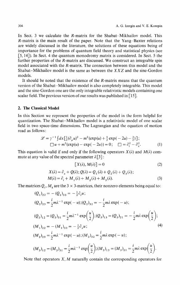
In Sect. 3 we calculate the ^-matrix for the Shabat-Mikhailov model. Thisi^-matrix is the main result of the paper. Note that the Yang-Baxter relationsare widely discussed in the literature, the solutions of these equations being ofimportance for the problems of quantum field theory and statistical physics (see[5,14]). In Sect. 4 the quantum monodromy matrix is considered. In Sect. 5 thefurther properties of the ^-matrix are discussed. We construct an integrable spinmodel associated with the K-matrix. The connection between this model and theShabat-Mikhailov model is the same as between the XX Z and the sine-Gordonmodels.

It should be noted that the existence of the i^-matrix means that the quantumversion of the Shabat-Mikhailov model is also completely integrable. This modeland the sine-Gordon one are the only integrable relativistic models containing onescalar field. The previous version of our results was published in [15].

2. The Classical Model

In this Section we represent the properties of the model in the form helpful forquantization. The Shabat-Mikhailov model is a relativistic model of one scalarfield in two space-time dimensions. The Lagrangian and the equation of motionread as follows:

• u + m2(exp(w) — exp( — 2u)) = 0; D = df — d^. (1)

This equation is valid if and only if the following operators X(λ) and M(λ) com-mute at any value of the spectral parameter λ [3] :

[X(λ),M(λ)] = 0 (2)

X(λ) = dχ + Q(λ); Q(λ) = Q, (λ) + Q2 (λ) + β 3 (λ)

M(λ) = dt + M, (λ) + M 2 (A) + M 3 (λ). (3)

The matrices β., Mk are the 3 x 3-matrices, their nonzero elements being equal to:

(Q 2 ) 2 3 =-mλ~ι exp( — w);(Q2)32 = —-mAexp( — M);

(δ3)i2 = ( β 3 ) 3 i = i m A " 1 1

( M 2 ) 2 3 = l-mλ~x exp( - u); ( M 2 ) 3 2 = -mλ exp( - M);

Note that operators X, M naturally contain the corresponding operators for

Quantum Shabat-Mikhailov Model 305

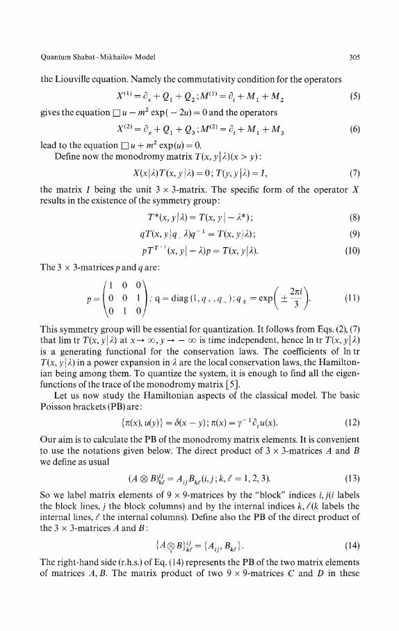
the Liouville equation. Namely the commutativity condition for the operators

χ ί 2 dt + M1+M2 (5)

gives the equation \Z\u — m2 exp( — 2u) = 0 and the operators

X(2) = dχ + Qi+Q3 ; M(2) = Qt + ^ + M s ( 6 )

lead to the equation C\u + rn2 exp(w) = 0.Define now the monodromy matrix T(x, y \ λ)(x > y):

X(x\λ)T(x9y\λ) = O;T{y9y\λ) = I9 (7)

the matrix I being the unit 3 x 3-matrix. The specific form of the operator Xresults in the existence of the symmetry group:

T*{x9y\λ)=T(x9y\-λ*); (8)

qT(x9y\q_λ)q'1 = T(x9y\λ); (9)

pTτ-\x9y\-λ)p=T{x9y\λ). (10)

The 3 x 3-matrices p and q are:

/I 0 0\ / 2 Λp = 0 0 1 ) ; q = diag( l ,^ + ,^_) ;^ + =exp( ± - ^ Y (11)

\0 1 0/ V 7

This symmetry group will be essential for quantization. It follows from Eqs. (2), (7)that lim tr T(x, y \ λ) at x -> oo, y -» — oo is time independent, hence In tr T(x, 3; | λ)is a generating functional for the conservation laws. The coefficients of In trT(x, y I λ) in a power expansion in /I are the local conservation laws, the Hamilton-ian being among them. To quantize the system, it is enough to find all the eigen-functions of the trace of the monodromy matrix [5].

Let us now study the Hamiltonian aspects of the classical model. The basicPoisson brackets (PB) are:

{π(x\ u(y)} = δ(x - y) π(x) = y~%u{x). (12)

Our aim is to calculate the PB of the monodromy matrix elements. It is convenientto use the notations given below. The direct product of 3 x 3-matrices A and Bwe define as usual

(A ® B)% = A^BJίJ K^=1,2, 3). (13)

So we label matrix elements of 9 x 9-matrices by the "block" indices i,j(i labelsthe block lines, j the block columns) and by the internal indices /c, *f(fc labels theinternal lines, *f the internal columns). Define also the PB of the direct product ofthe 3 x 3-matrices A and B:

{Λ®B}%={AipBj. (14)

The right-hand side (r.h.s.) of Eq. (14) represents the PB of the two matrix elementsof matrices A, B. The matrix product of two 9 x 9-matrices C and D in these


notations can be written as:

(ΓD)ij — CίmDmj (\5)

The summing up by the repeated indices is implied here.To calculate the required PB we use the trick based on the classical r-matrix.

If one succeeds in representing the PB of the matrix elements of Q (Eq. (3)) asfollows:

{Q(x\λ)ΘQ(y\μ)} = yδ(x-y)[r(λ,μlQ(x\λ)®I + I®Q(x\μ)'] (16)

then the PB of the monodromy matrix elements can be written as:

{T(x9y\λ)®T(x9y\μ)} = -y[]ίλ9μ)9T(x9y\λ)®T(x9y\μ)l (17)

We give a particularly simple derivation of this formula in Appendix I. The squarebrackets at the r.h.s. of (16), (17) denote the commutator of two 9 x 9-matrices;r is a numerical 9 x 9-matrix with elements depending on λ and μ. The existenceof the r-matrix in (16) is not a priori evident. The direct calculation by means of(3), (4), (12) confirms, however, the validity of (16). We put the matrix r into theform:

3

r= Σ r*meik®e€m.i,k,J,m=l

The 3 x 3-matrices eik form the standard basis, their matrix elements being equalto:

(eik)ab = δiaδkh (18)

The matrix r depends on λ/μ = exp(β) only: r(λ,μ) = r(β). The non-zero matrixelements are:

r\\ = (2 - exp(3/?) - exp( - 3β))g(β);

Λϊ = rϊϊ = Λ\ = Λ\ = ~*•" = rl32 = ~ 2(exp(3

r\\ = r3i = 2(exp(2/?) + exp( - β))g(β);

r\\ = r\\ = 2(exp(2^) - exp( - β))g(β); (19)

r\\ = r\\ = 2(exp(^) + exp( - 2β))g(β);

r\\ = r\\ = 2(exp( - 2β) - exp(/ί))#(/?);

r\\ = 4 cxp(2β)g(β);r3

2

2

3 = 4 exp( - 2β)g(β)

exp( - 3β))g(β);

The classical r-matrix is defined up to the addition of the arbitrary matrixproportional to the unit 9 x 9-matrix E (see Eq. (16)).

The expression for the PB of the monodromy matrix elements is the mainresult of this Section. These formulae also determine the PB of the scattering data.

3. The Quantum /?-Matrix

In this Section we consider the quantum version of the Shabat-Mikhailov model


in the framework of the quantum inverse scattering method. The quantum modelis given by the Lagrangian in (1) and the following commutation relations (CR)of the operators u(x) and π(x) = y~ί dtu(x):

[π(x),u(y)-]=-iδ(x-y). (20)

We will pay attention to the CR of the elements of the quantum monodromymatrix t(x9y\λ)9 this matrix being of importance also in the quantum inversescattering method. For completely integrable quantum systems the followingrelation is valid [11,5]:

R(λ, μ)(f(x9 y\λ) (x) f(χ, y \μ)) = (f(x,y\μ) ® t(x9 y\λ))R(λ, μ). (21)

This relation is similar to (17) for the classical model. The elements of the 3 x 3 -matrix t are quantum operators and R(λ, μ) is a numerical 9 x 9-matrix, dependingalso on y.

Our purpose in this Section is to calculate the quantum K-matrix for the model.Note that (21) results in the following system of equations for R{λ,μ) (seeAppendix 2):

(/ <g> R(λ9 μ)){R(λ9 v) ® /)(/ <g> Λ(μ, v))

® R(λ9 v))(K(λ, μ) ® I). (22)

The 27 x 27-matrix (/ (x) R) is a direct product of the 3 x 3-unit matrix / and 9 x 9 -matrix R. Hence the l.h.s. and r.h.s. of Eq. (22) contain the ordinary matrix productof three 27 x 27-matrices. Eq. (22) can be written in the explicit form as follows:

RZI& »)*'£& v)KtzMv) = RZ'M »)«S:^ WclllV* /*)• (23)These equations are the famous Yang-Baxter relations. Equations (22) and (23)are the basic ones for the calculation of the jR-matrix.

A number of additional restrictions should be imposed on the .R-matrix. Therelativistic invariance implies that

R(λ9μ) = R(λ/μ). (24)

The quasiclassical limit of .R is determined by the classical r-matrix. Comparing(17) and (21) one can obtain:

R(λ/μ)~Rc(λ/μ);

c = P(E-ίyr(λ/μ)). (25)

The 9 x 9 permutation matrix P is defined by

and has the following properties

Here C, D are the numerical 3 x 3-matrices. Notice that the symmetries (Eqs. (8),(9), (10)) of the matrix T result in the existence of the symmetry properties of thematrix jR . We require these symmetries to be the same for the exact quantum


matrix JR :

(q-1 ® q-1)R(λ/μ)(q®q) = R(λ/μ); (27)

(/ ® q~ 1 )R(λ/μ)(q ® J) = R(q_λ/μ) (28)

PR*{λ/μ)P = R(μ*/λ*); (29)

PR(λ/μ)P = (p ® p)KΓ(i/μ)(/7 ® p). (30)

This requirement means that the classical symmetries survive after quantization.It is shown in Sect. 4 that the symmetries of T(x, y \ λ) agree with Eqs. (27)-(30).Eq. (21) shows that the jR-matrix is determined up to a scalar factor f(λ, μ). Wechoose this function/implying the conditions:

22 1. (31)

Now we have written down all the equations which determine matrix R.We succeeded in finding the ̂ -matrix satisfying all these equations [15]. This

matrix can be represented as the product of five 9 x 9-matrices:

R(λ/μ;φ) = (I ® fl(λ/μ))LΓ' (φ) D(λ/μ φ)U{φ){a-\λ/μ) ® /)

φ^yβ (32)

We use the following notations. The elements of the diagonal matrix D is equal to

D\\ = cosh((3β/2) + 3ί»/cosh((3β/2) - 3iφ);n i l _ D 2 2 _ r)33

33 — 11 — 22

= - sinh((3j3/2) + 2iφ)/sinh((3iS/2) - 2iφ) ( 3 3 )

D» = D\\ = D\\ = D\\ = D\\ = \ λ/μ = exp(^).

The nonzero elements of the matrix U(φ) are:

= - U[l = - Ul\ = - υ\\ = U\l = exp ( - iφ) (34)= Qxp{2ίφ); U\\ = exp( —

U\\ =

The diagonal 3 x 3-matrix a{x) is:

a(x) = diag(l, x, X" ̂ αμ/μ) = flix)|x=^. (35)

The nonzero matrix elements of the matrix R are situated at the same places asthe nonzero matrix elements of the matrix U.

The explicit expression for the matrix R is our principal result.Let us make now some remarks. It follows from the explicit expression of the

.R-matrix that it also possesses the following additional symmetries:

RT = R; (36)

(a(x)®a(x))R(λ/μ; φ) = R(λ/μ; φ)(a(x) ® a(x)); xeC. (37)


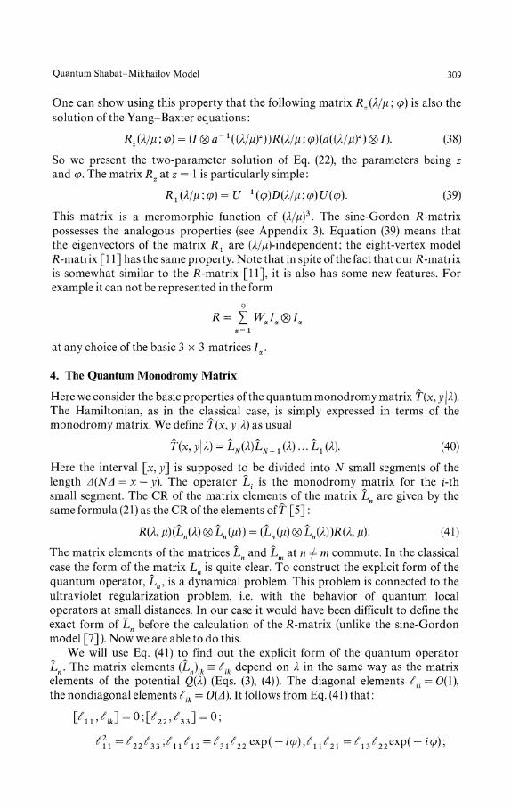
One can show using this property that the following matrix Rz(λ/μ; φ) is also the

solution of the Yang-Baxter equations:

Rz(λ/μ ;φ) = (I®a- '((λ/'μ)z))R(λ/'μ φ)(a((λ/μ)z) ® I). (38)

So we present the two-parameter solution of Eq. (22), the parameters being zand φ. The matrix Rz at z = 1 is particularly simple:

R1(λ/μ;φ)=U-1(φ)D(λ/μ;φ)U(φ). (39)

This matrix is a meromorphic function of (λ/μ)3. The sine-Gordon JR-matrixpossesses the analogous properties (see Appendix 3). Equation (39) means thatthe eigenvectors of the matrix Rι are (/l/μ)-independent; the eight-vertex modelK-matrix [11] has the same property. Note that in spite of the fact that our jR-matrixis somewhat similar to the K-matrix [11], it is also has some new features. Forexample it can not be represented in the form

at any choice of the basic 3 x 3-matrices Jα.

4. The Quantum Monodromy Matrix

Here we consider the basic properties of the quantum monodromy matrix f(x, y\λ).The Hamiltonian, as in the classical case, is simply expressed in terms of themonodromy matrix. We define T(x, y | λ) as usual

T(x, y\λ) = LN(λ)LN_ χ (λ)... Lγ (A). (40)

Here the interval [x, y\ is supposed to be divided into N small segments of thelength Δ(NΔ = x — y). The operator L. is the monodromy matrix for the z-thsmall segment. The CR of the matrix elements of the matrix Ln are given by thesame formula (21) as the CR of the elements of f [5] :

R(λ, μ)(Ln(λ) (x) Ln(μ)) = ( L » ® Ln{λ))R(λ, μ). (41)

The matrix elements of the matrices Ln and Lm2Ltnφm commute. In the classicalcase the form of the matrix Ln is quite clear. To construct the explicit form of thequantum operator, Ln, is a dynamical problem. This problem is connected to theultraviolet regularization problem, i.e. with the behavior of quantum localoperators at small distances. In our case it would have been difficult to define theexact form of Ln before the calculation of the JR-matrix (unlike the sine-Gordonmodel [7]). Now we are able to do this.

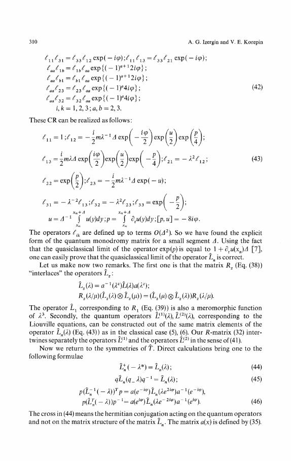
We will use Eq. (41) to find out the explicit form of the quantum operatorLn. The matrix elements (Ln)ik = ^ίk depend on λ in the same way as the matrixelements of the potential Q(λ) (Eqs. (3), (4)). The diagonal elements £{i = 0(1),the nondiagonal elements ίik = 0{A). It follows from Eq. (41) that:


(42)

ί,/c=l,2,3;α,b = 2,3.

These CR can be realized as follows:

ϋexp(J jexpί |

U\3=-mλΔ exp -£ exp - exp -"- V/21 = - λ V 1 2 ; (43)

t?22 = expl-J'/23=-^mλ ^Qxpi-u);

xn + A xn + A

u = A~1 j u(y)dy;p= \ dtu(y)dy [p, u] =- Sίφ.xn xn

The operators £ik are defined up to terms 0(A2). So we have found the explicitform of the quantum monodromy matrix for a small segment A. Using the factthat the quasiclassical limit of the operator exp(p) is equal to 1 + dtu{xn)A [7],one can easily prove that the quasiclassical limit of the operator Ln is correct.

Let us make now two remarks. The first one is that the matrix Rz (Eq. (38))"interlaces" the operators L :

Rz(λ/μ)(Lz(λ)®Lz(μ)) = {Lz(μ)®Lz{λ))Rz{λ/μ).

The operator L1 corresponding to R1 (Eq. (39)) is also a meromorphic functionof λ3. Secondly, the quantum operators La)(λ\ L{2\λ\ corresponding to theLiouville equations, can be constructed out of the same matrix elements of theoperator Ln(λ) (Eq. (43)) as in the classical case (5), (6). Our H-matrix (32) inter-twines separately the operators L(1) and the operators L(2) in the sense of (41).

Now we return to the symmetries of T. Direct calculations bring one to thefollowing formulae

L+

n(-λ*) = Ln(λ); (44)

qLn(q_λ)q-ι = Ln(λ); (45)

p{L-\- λ))τp = aie-'nhiλe^a-He-*),

p(Ll( - λ))p~ ι= aie^L^λe-^ηa-1^). (46)

The cross in (44) means the hermitian conjugation acting on the quantum operatorsand not on the matrix structure of the matrix Ln. The matrix a(x) is defined by (35).


It follows from Eq. (40) that the monodromy matrix f possesses literally the sameinvolutions as the matrix Ln. The action of the symmetry group (44), (45), (46)turns into the classical one (8), (9), (10) in the quasiclassical limit φ -> 0. The sym-metry properties of the ^-matrix (Eqs. (27)-(30)) and of the matrix T (Eqs. (44)-(46)) agree with the Eq. (21) due to Eqs. (37), (24).

In this paper we will not discuss the properties of the quantum .monodromymatrix in more detail, expecting to return in another paper to the constructionof Bethe Ansatz, the physical vaccum and mass spectrum for the model.

5. The Properties of the /WVίatrix

In this Section we describe the lattice model associated with the .R-matrix definedby (32) and construct the Zamolodchikov-Cherednik operators Λa(λ) for thismatrix.

First of all we describe the completely integrable lattice model, the constructionof this model being similar to the construction of Baxter's eight-vertex model[11,14]. For this purpose we rewrite the "trilinear" relation (22) in the "bilinear"form similar to (41). Let us introduce nine 3 x 3-matrices Lb

a (the indices α, b =1, 2, 3 enumerate the matrices as a whole). We shall regard each individual matrixLb

a as the "quantum operator". The matrices Lb

a are defined as follows:

(L"a(λ)i = R%(λ). (47)

Here i,k= 1,2,3 are matrix (quantum) indices of the matrix Lb

a. Using thesenotations one can put Eq. (22) into the form similar to (41):

% % £ #j(λ/μ). (48)

Equation (48) shows that the operators Lb

a form in a natural way the 3 x 3-matrix Lwhich is similar to the matrix Ln from (40), (43). It should be noted that it wasconvenient for us to prove the validity of Eq. (22) in the form (48).

Equation (48) shows that the following model on the square N x M periodictwo-dimensional lattice is integrable; the transfer-matrix τ of the model is definedas

τ(λ)= Σ (^WC^^-iWζ:;-^!^))^- (49)ai...aN

The main property of this transfer-matrix is

The partition function Z is expressed as usual:

Z = Sp τ M

(our notation for the transfer matrix differs from the notation in [14]). τ is anoperator in the "quantum" space, in other words τ is the 3N x

This lattice model generates in a standard way [16] the integrable spin modelon the one-dimensional periodic lattice with N sites. The Hamiltonian of the


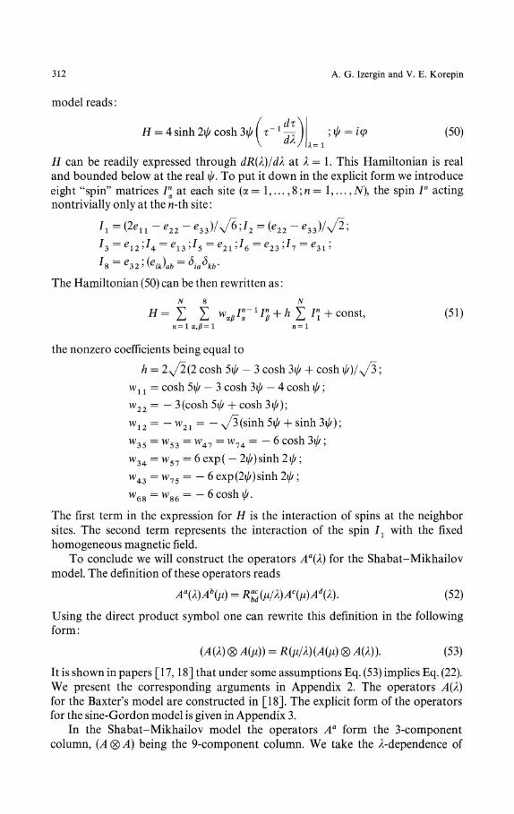
model reads:

H = 4 sinh 2ψ cosh 3φ ( τ 1 -jτUA

(50)λ=l

H can be readily expressed through dR{λ)/dλ at λ = 1. This Hamiltonian is realand bounded below at the real φ. To put it down in the explicit form we introduceeight "spin" matrices /" at each site (α = 1,..., 8 n = 1,..., N), the spin Γ actingnontrivially only at the n-th site:

h =

The Hamiltonian (50) can be then rewritten as:

#= Σ Σ V Γ 1 ^ * ! 7" + c o n s t 'n=lα,/?=l «=1

the nonzero coefficients being equal to

h = 2^/2(2 cosh 5φ — 3 cosh 3^ + cosh φ) 1-^/3

wx t = cosh 5φ — 3 cosh 3φ — 4 cosh i/f

w 2 2 = — 3 (cosh 5i/f + cosh 3^);

w 1 2 = — w2 1 = — ̂ /3(sinh 5^ + sinh3ι//);

w 3 4 = w 5 7 = 6exp( —

w 4 3 = w7 5 = — 6 exp(2ι^)sinh

The first term in the expression for H is the interaction of spins at the neighborsites. The second term represents the interaction of the spin / 1 with the fixedhomogeneous magnetic field.

To conclude we will construct the operators Λa(λ) for the Shabat-Mikhailovmodel. The definition of these operators reads

Aa{λ)A\μ) = Ra

b

c

d(μ/λ)Ac(μ)Ad(λ). (52)

Using the direct product symbol one can rewrite this definition in the followingform:

(A(λ) (x) A(μ)) = R(μ/λ)(A(μ) ® A(λ)). (53)

It is shown in papers [17,18] that under some assumptions Eq. (53) implies Eq. (22).We present the corresponding arguments in Appendix 2. The operators A(λ)for the Baxter's model are constructed in [18]. The explicit form of the operatorsfor the sine-Gordon model is given in Appendix 3.

In the Shabat-Mikhailov model the operators Aa form the 3-componentcolumn, (A ® A) being the 9-component column. We take the /l-dependence of


A(λ) in the following form:

A1(λ) = A1;

Equation (53) is then reduced to the following relations:

Aγa = aA

x exp(2iφ); A

χb = bA

1 exp( — 2ίφ);

Aγc = cA

ί Qxp(-2iφ); be = cbexp(4ίφ);

ac = ca exp( — 4iφ); ab = ba;

Al = (exp(3iφ) + exp(iφ))αc.

These relations can be realized by means of operators acting on the scalar functionsof one variable,/(x):

AJ(x) = m exp(zx x)f(x + a1);

A2f(x) = λ Qxp(z2x)f(x + a2) + ρλ~2 exp( - z2x)f(x -a2); (54)

AJ{χ) = λ'1 exp(z3x)/(x + α 3);

m2 = (exp(3ι» + exp(ί»)exp(α2z3 — a1z1).

Here p is an arbitrary constant and the parameters α., z. satisfy the followingequations:

2aί = a2 + a3; 2z1 = z2 + z3; z2a3 — a2z3 = 4iφ.

The formula (54) gives the explicit realization of the operators Aa.

Appendix 1

The monodromy matrix T(x9y\λ) depends on dynamical variables u{x\ π(x)through the potential Q(x|λ) only. So one can express the Poisson brackets ofthe monodromy matrix elements as follows:

{Ttμ\ Tk({μ)} = μzJd^^μ

•(δTk,(x,y\μ)/δQJzy

μ\μ)){QJzλ\λ),QJzμ\μ)}. (Al)

One can calculate the variational derivative of T(λ) with respect to Q(λ) by meansof the perturbation theory:

δT(x,y\λ)=-]τ(x9z\λ)δQ(z\λ)T(z9y\λ)dz. (A2)y

Now it is possible to rewrite (Al) by means of (A2) and (13), (14), (15) in the elegantform:

•{Q(z>\λ)®Q{zlι\μ)}{T{zvy\λ)®T(zlι,y\μ)). (A3)


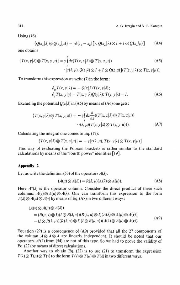
Using (16)

{Q(zλ\λ)<$Q{zμ\μ)} = yδ(zλ - zμ)\τ9 Q(zλ\λ)®I + / ® β ( z » ] (A4)

one obtains

{T(x9y\λ)<$T(x9y\μ)} = y]dz(T(x9z\λ)®T(x9z\μ)) (AS)

To transform this expression we write (7) in the form:

dxT(x9y\λ)=-Q(x\λ)T(x9y\λ);

dyT(x, y\y) = T(x9 y\λ)Q(y\λ); T(y9y\λ) = L (A6)

Excluding the potential Q(z\λ) in (A5) by means of (A6) one gets:

{T(x9y\λ)®T(x9y\μ)} = -γ]dz^((T(x9z\λ)®T(x9z\μ))

-r(λ9μ)(T(z9y\λ)®T(z9y\μ))). (A7)

Calculating the integral one comes to Eq. (17):

{T{x9y\λ)<$T(x9y\μ)}=-γlr(λ9μ)9T(x9y\λ)®T(x9y\μ)-]

This way of evaluating the Poisson brackets is rather similar to the standardcalculations by means of the "fourth power" identities [19].

Appendix 2

Let us write the definition (53) of the operators A(λ):

(A(μ) ® A(λ)) = R(λ, μ)(A (λ) (x) A(μ)). (A8)

Here Aa(λ) is the operator column. Consider the direct product of three suchcolumns: A(v)(x)A(μ)(x)A(λ). One can transform this expression to the formA(λ) (x) A(μ) (x) ̂ 4(v) by means of Eq. (A8) in two different ways:

{A(v)®A{μ)®A(λ))

= (R(μ, v) ® /)(/ ® R(λ, v))(R{λ9 )

= (/ ® R(λ9 μ))(R(λ, v) ® /)(/ ® R(μ, v))(A{λ) ® A(μ) ® ̂ (v)). ( }

Equation (22) is a consequence of (A9) provided that all the 27 components ofthe column ^4®^1®^4 are linearly independent. It should be noted that ouroperators Aa(λ) from (54) are not of this type. So we had to prove the validity ofEq. (22) by means of direct calculations.

Another way to obtain Eq. (22) is to use (21) to transform the expressionT(λ) ® T(μ) ® T(v) to the form T(v) ® T(μ) ® T(λ) in two different ways.


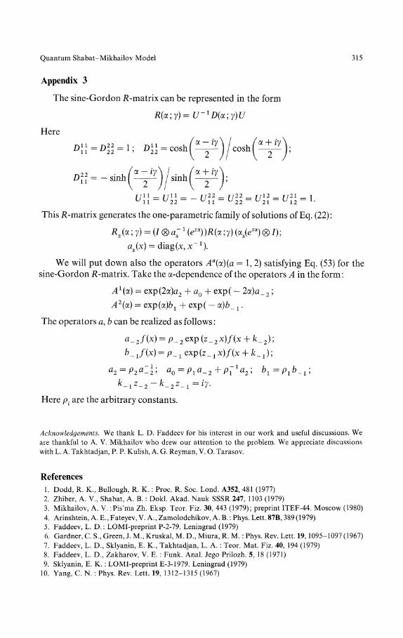
Appendix 3

The sine-Gordon K-matrix can be represented in the form

R(x;γ)=U-1D(z;γ)U

Here

iγ

This K-matrix generates the one-parametric family of solutions of Eq. (22):

a;ι (

We will put down also the operators Aa(a)(a =1,2) satisfying Eq. (53) for thesine-Gordon β-matrix. Take the α-dependence of the operators A in the form:

A1 (a) = exp(2α)α2 + a0 + exp( - 2oc)a_2

^42(α) = Qxp(oc)bί + exp( — α)fc_ 1.

The operators α, b can be realized as follows:

α_2/(x)-p_2exp(z_2x)/(x + fe_2);

b-i/W = P-! exp(z_ 1 x)/(χ + fc_ Jβ

2

= P 2 α - 2 ' ao = p1a_2 + p;1a2; b1=ρίb_i;

k_1z_2-k_2z_1 =iγ.

Here pt are the arbitrary constants.

Acknowledgements. We thank L. D. Faddeev for his interest in our work and useful discussions. We

are thankful to A. V. Mikhailov who drew our attention to the problem. We appreciate discussions

with L. A. Takhtadjan, P. P. Kulish, A. G. Reyman, V. O. Tarasov.

References1. Dodd, R. K., Bullough, R. K.: Proc. R. Soc. Lond. A352, 481 (1977)

2. Zhiber, A. V., Shabat, A. B.: Dokl. Akad. Nauk SSSR 247, 1103 (1979)

3. Mikhailov, A. V. Pis'ma Zh. Eksp. Teor. Fiz. 30, 443 (1979); preprint ITEF-44. Moscow (1980)

4. Arinshtein, A. E., Fateyev, V. A., Zamolodchikov, A. B.: Phys. Lett. 87B, 389 (1979)

5. Faddeev, L. D.: LOMI-preprint P-2-79. Leningrad (1979)

6. Gardner, C. S., Green, J. M., Kruskal, M. D., Miura, R. M. : Phys. Rev. Lett. 19,1095-1097 (1967)

7. Faddeev, L. D., Sklyanin, E. K., Takhtadjan, L. A. : Teor. Mat. Fiz. 40, 194 (1979)

8. Faddeev, L. D., Zakharov, V. E.: Funk. Anal. Jego Prilozh. 5, 18 (1971)

9. Sklyanin, E. K. : LOMI-preprint E-3-1979. Leningrad (1979)

10. Yang, C. N. : Phys. Rev. Lett, 19, 1312-1315 (1967)


11. Baxter, R. J. : Ann. Phys. (NY). 70, 193-228 (1972); 70, 323-327 (1972); 76, 25-47 (1973); 76,48-71 (1973)

12. Zamolodchikov, A. B.: Commun. Math. Phys. 55, 183 (1977)13. Karowski, M.,Thun, H. J.,Truong,T. T., Weisz, P. H.: Phys. Lett. 67B, 321-322(1977)14. Faddeev, L. D., Takhtadjan, L. A.: Usp. Mat. Nauk. 34, 13-63 (1979)15. Izergin, A. G., Korepin, V. E.: LOMI-preprint E-3-80. Leningrad (1980)16. Sutherland, B.: J. Math. Phys. (NY), 11, 3183-3186 (1970)17. Zamolodchikov, A. B.: Pis'ma Zh. Exp. Teor. Fiz. 25, 499-502 (1977)18. Cherednik, I. V. Dokl. Akad. Nauk SSSR 249, 1095 (1979)19. Zakharov, V. E., Manakov, S. V., Novikov, S. P., Pitajevsky, L. P. :The theory of solitons.

Moscow: Nauk 1980

Communicated by Ya. G. Sinai

Received July 14, 1980

the inverse scattering method approach to the quantum

Documents