the inﬂuence of watershed characteristics on …. steinberg_etal_2011... · the inﬂuence of...

The influence of watershed characteristics on nitrogenexport to and marine fate in Hood Canal, Washington, USA

Peter D. Steinberg • Michael T. Brett •

J. Scott Bechtold • Jeffrey E. Richey •

Lauren M. Porensky • Suzanne N. Smith

Received: 15 April 2009 / Accepted: 23 August 2010 / Published online: 21 October 2010

� Springer Science+Business Media B.V. 2010

Abstract Hood Canal, Washington, USA, is a poorly

ventilated fjord-like sub-basin of Puget Sound that

commonly experiences hypoxia. This study examined

the influence of watershed soils, vegetation, physical

features, and population density on nitrogen (N) export

to Hood Canal from 43 tributaries. We also linked our

watershed study to the estuary using a salinity mass

balance model that calculated the relative magnitude of

N loading to Hood Canal from watershed, direct

precipitation, and marine sources. The overall flow-

weighted total dissolved N (TDN) and particulate N

input concentrations to Hood Canal were 152 and

49 lg l-1, respectively. Nitrate and dissolved organic

N comprised 64 and 29% of TDN, respectively.

The optimal regression models for TDN concentration

and areal yield included a land cover term suggesting an

effect of N-fixing red alder (Alnus rubra) and a human

population density term (suggesting onsite septic

system (OSS) discharges). There was pronounced

seasonality in stream water TDN concentrations,

particularly for catchments with a high prevalence of

red alder, with the lowest concentrations occurring in

the summer and the highest occurring in November–

December. Due to strong seasonality in TDN concen-

trations and in particular stream flow, over 60% of the

TDN export from this watershed occurred during the

3 month period of November–January. Entrainment of

marine water into the surface layer of Hood Canal

accounted for &98% of N loading to the euphotic zone

of this estuary, and in a worst case scenario OSS N

inputs contribute &0.5% of total N loading. Domestic

wastewater discharges and red alders appear to be a

very important N source for many streams, but a minor

nutrient source for the estuary as a whole.

Keywords Hood Canal � Puget Sound �Stream chemistry � Nitrogen � Red alder �Onsite septic systems � Eutrophication � Hypoxia

Introduction

Since the Industrial Revolution, human activities

have doubled the loading of mineralized nitrogen (N)

to terrestrial ecosystems (Vitousek et al. 1997;

P. D. Steinberg � M. T. Brett (&) � S. N. Smith

Department of Civil Engineering,

University of Washington, Box 352700,

Seattle, WA 98195-2700, USA

e-mail: [email protected]

J. S. Bechtold

School of Aquatic and Fishery Sciences,

University of Washington, Box 355020,

Seattle, WA 98195-5020, USA

J. E. Richey � L. M. Porensky

School of Oceanography, University of Washington,

Box 355351, Seattle, WA 98195-7940, USA

P. D. Steinberg (&)

GoldSim Technology Group, 300 NE Gilman Blvd,

Suite 100, Issaquah, WA 98027-2941, USA

e-mail: [email protected]

123

Biogeochemistry (2011) 106:415–433

DOI 10.1007/s10533-010-9521-7

Green et al. 2004). On a global scale the most

significant anthropogenic inputs to the reactive N

cycle include fertilizers, wastewater discharges, urban/

suburban runoff, and NOx and NH3 loading to the

atmospheric from fossil fuel combustion and agricul-

ture (Vitousek et al. 1997; Paerl et al. 2002; Galloway

et al. 2004). Excessive terrestrial N loading can lead to

soil N saturation, decreased tree productivity,

enhanced N leaching into surface and groundwaters

(Fenn et al. 1998), and in some cases dramatically

increased loading to receiving lakes, rivers and estu-

aries (Howarth et al. 1996; Boyer et al. 2006).

Intact conifer-dominated watersheds are usually N

limited (Sollins et al. 1980; Triska et al. 1984; Hedin

et al. 1995), discharge proportionally more dissolved

organic than inorganic N (Perakis and Hedin 2002),

and have low areal N yields (Perakis and Hedin 2002;

Cairns and Lajtha 2005). Areas subjected to timber

harvest and other disturbances are often re-colonized

by early successional nitrogen-fixing species such as

alder (Alnus spp.). Red alder (Alnus rubra), a prevalent

deciduous tree in the Pacific northwest region of North

America, can fix 100–200 kg N ha-1 year-1 (Binkley

et al. 1994). Since alders often grow in riparian areas

adjacent to surface and subsurface flow paths, high soil

and litterfall N concentrations can lead to increased

stream water N concentrations (Hurd et al. 2001;

Compton et al. 2003; Hurd and Raynal 2004).

Increased stream water N yields due to alders have

been noted in the coastal range of Oregon (Compton

et al. 2003), the Olympic Peninsula in Washington

(Bechtold et al. 2003), the Adirondack Mountains in

New York (Hurd et al. 2001; Hurd and Raynal 2004),

forests of Wisconsin (Younger and Kapustka 1983),

and fens in Germany (Busse and Gunkel 2002).

Our study was initiated as part of a broader effort

to understand hypoxic events and associated fish-kills

in Hood Canal. Hood Canal is an N-limited, deep,

stratified fjord-like sub-basin of the Puget Sound

estuary with a shallow sill blocking deep-water tidal

exchange at its marine boundary (Newton et al.

1995). Dissolved oxygen (DO) concentrations in

the deep waters of Hood Canal decline during the

summer due to strong density stratification and

the settling/decomposition of phytoplankton from

the euphotic zone, and low summer/fall DO concen-

trations have been observed since the 1950s (Collias

et al. 1974). Nearly all of the lower reaches of the

Hood Canal watershed have been logged or cleared at

least once, and are dominated by red alders. Further-

more, while population density in the Hood Canal

watershed is quite low, i.e., \20 individuals km-2,

much of the population is concentrated along the

shorelines, and all domestic wastewater discharges

within the watershed are treated by on-site septic

(OSS) systems.

The overall objectives of our study were to

determine the loading of dissolved nitrogen by source

into Hood Canal, and to assess that loading relative to

marine sources. We examined the extent to which

watershed characteristics (e.g., soils, land cover,

physical features and population density) predict

stream water N concentrations and nutrient export to

Hood Canal from its tributaries. We then linked the

watershed to the Canal, using a salinity mass balance

to estimate marine upwelling flows, and assessed the

magnitudes of watershed N export to the surface

mixed layer of Hood Canal relative to marine sources

(i.e., estuarine circulation).

Study area

The Hood Canal (Fig. 1) watershed has a surface area

of *3,050 km2, of which Hood Canal itself comprises

12%. The watershed can be separated into three zones:

(1) the large snowmelt dominated catchments of the

Olympic Mountains, (2) the Skokomish River, and (3)

the many smaller rain dominated catchments of the

Kitsap Peninsula and Hood Canal lowlands. Dominant

land uses/covers in the lowland catchments are

re-growth conifer, deciduous mixed forests, and sub-

urban and semi-rural development (Table 1). Areas

mapped as deciduous mixed forest usually have a

closed upper canopy that is composed of ca. 50% red

alder (L. Porensky, unpubl. data). The upper elevations

are within the Olympic National Park and are nearly

pristine conifer forests. The middle elevations are part

of Olympic National Forest, 76% of which has been

logged (Peterson et al. 1997).

The lowland catchments have more disturbance

from forest clearing, wetland draining and suburban

development. In this watershed, over 60% of precip-

itation occurs between November and January and less

than 10% occurs between June and August. Freshwater

inputs to Hood Canal averaged 170 m3 s-1 during the

water years 1990 to 2006. The first study year (i.e.,

2005) was somewhat drier than average, whereas 2005

416 Biogeochemistry (2011) 106:415–433

123

Fig. 1 Map showing the

location of the 43 sampled

tributaries in the Hood

Canal watershed,

Washington

Table 1 Physical characteristics, and land cover and soil types for the five regions of the Hood Canal watershed

Skokomish

RiveraDiversion from

North Fork

Skokomish

Other Olympic

Mountain

catchments

Sampled

Kitsap/lowland

catchments

Unsampled

Kitsap/lowland

catchments

Physical characteristics

Catchment area (km2) 375 254 985 578 618

Mean elevation (m) 428 808 543 186 118

Average slope (%) 40.2 52.9 44.0 14.8 17.1

Average discharge (1990–2006) (m3 s-1) 37.6 21.9 69.5 19.6 20.7

Average runoff (1990–2006) (m year-1) 3.2 2.7 2.2 1.1 1.1

Population density (people km-2) 3.6 3.8 3.8 20 45

Land cover

Mature coniferous forest (%) 46.4 58.3 49.9 41.3 23.7

Deciduous mixed forest (%) 8.8 3.8 7.3 16.9 29.3

Grass/shrubs/crops/early regrowth (%) 8.6 5.3 7.6 8.1 9.4

Young coniferous forest (%) 9.7 3.6 7.9 13.3 15.1

Low and high density urban (%) 1.4 0.9 1.3 2.2 4.6

Soil types

Entisols (weakly developed soils)

not derived from till

41.3 64.5 45.3 38.3 51.0

Soils influenced by ash (andic soils

and andisols)

56.2 45.4 53.0 6.5 15.1

Soils derived from glacial till 13.8 12.5 13.4 49.5 29.7

Rock outcrops 6.4 14.4 8.8 0.1 0.0

a Skokomish River does not include that area of the North Fork Skokomish River upstream of upstream of Cushman Dam

Biogeochemistry (2011) 106:415–433 417

123

was the wettest year in the last 50. Average annual

runoff ranges from 3.2 m year-1 in the Skokomish

River catchment to 1.1 m year-1 in the lowlands

(Table 1). The mountainous areas of the watershed are

sparsely populated (i.e., &4 people km-2), and the

lowlands have moderate population densities

(&20 people km-2) with areas of higher population

density along the shoreline especially within Lynch

Cove (Table 1).

Methods

Basin attributes

A USGS 30 m resolution digital elevation model

(DEM) was used to create the stream network,

delineate catchment boundaries, and calculate

watershed areas, mean elevation and slope. Soils

data (SSURGO 2006) were used to construct a soil

matrix of chemical and physical characteristics and

taxonomic information for each soil type. Land

cover was classified, via a supervised classification

of a 30 m resolution Landsat Enhanced Thematic

Mapper Plus (ETM?) image from July 30, 2000

(NASA Landsat Program 2001), with at least 10

ground-truth reference sites used for each the land

cover type. Urban areas were masked based on their

location in the PRISM 2002 landcover map (Alberti

et al. 2004), and subalpine forests were masked

based on their proximity to snow-covered areas. To

estimate this land cover classification’s accuracy,

100 randomly located test points were referenced

against aerial photographs from 2003, which sug-

gested that the final product had a classification

accuracy of [90%.

Population estimates for each catchment were

generated by disaggregating 2000 US Census block

data using normalized difference vegetation index

(NDVI) scores (sensu Imhoff et al. 2000; Koh et al.

2006), derived from the previously mentioned Land-

sat image. The PRISM 2002 land cover classification

was used to subdivide the original NDVI raster into

three component rasters, including areas expected to

have zero population (e.g., steep slopes), suburban

areas (with 90% of the population) and rural areas

(with 10% of the population). Within the suburban

and rural rasters, the population for each census block

was divided among individual pixels based on the

difference between each pixel’s NDVI value and the

mean NDVI value of the census block.

Field and laboratory procedures

Forty-three streams, accounting for 88% of the overall

watershed’s hydrologic yield, were sampled monthly

from January 2005 to December 2006. The unsampled

areas of the watershed (which accounted for 22% of the

surface area and 12% of the hydrologic yield) consisted

of small, undifferentiated shoreline catchments. Grab

samples were collected in 0.1 M HCl acid-washed

bottles pre-rinsed with streamwater. Dissolved nutrient

samples (NO3-, NH4

?) were filtered through What-

man� cellulose acetate filters (0.45 lm pore size), and

analyzed on an Alpkem RFA/2 autoanalyzer. TDN was

measured on a Shimadzu DOC analyzer after filtering

through pre-combusted Whatman� GF/F glass fiber

filters (0.7 lm). For particulates, 100–600 ml of

stream water, depending on turbidity, was filtered

through GF/F filters. Particulates captured on the filters

were dried at 55�C for 24 h, acid-fumigated for 24 h,

re-dried at 55�C, and packed in tin capsules. The

samples were analyzed for N and C concentration at the

UC-Davis Stable Isotope Facility using a PDZEuropa

ANCA-GSL elemental analyzer.

Streamflow estimation

Fourteen of the 43 streams, which accounted for 68%

of the total watershed area, including all large Olympic

Mountain rivers, had daily mean flow records. The

ungaged areas were narrow shoreline catchments and

small to medium size tributaries entirely within the

lowlands. Streamflows for the ungaged catchments

were estimated by classifying each drainage by hydro-

climatic region and then applying the mean of the areal

daily runoff rates for a particular region.

Loading rates

Monthly freshwater dissolved nutrient loads to Hood

Canal were estimated by multiplying the monthly

mean streamflows by the actual monthly grab sample

concentrations for the 39 sampling sites that were

direct discharges (i.e., not upstream of other sample

locations) to Hood Canal accordingly: Loading =P

monthly conc. 9 mean monthly flow 9 30.4.

The flow-weighted mean concentrations were used


123

as the response variable in regression models, these

were calculated accordingly; flow-weighted concen-

tration =P

monthly conc. 9 mean monthly flow/P

mean monthly flow.

To fill-in missing data we used the three streams

which had the most similar monthly patterns com-

pared to the stream with the missing data to generate

regression based estimates for the missing value and

we then took the average of these estimates to

represent the missing data. Before the fill-in process,

the 24-month by 43-stream dissolved constituent

concentration matrices were 78% complete. The

monthly arithmetic mean of concentrations measured

in the four most populated Kitsap watersheds (Big

Beef, Seabeck, Tahuya, and Union) were used to

estimate each month’s concentration for the unsam-

pled portions of the Hood Canal watershed. These

streams had average population densities (49 peo-

ple km-2) and deciduous mixed forest (21%), which

were similar to those of the unsampled region

(46 people km-2 and 29%, respectively) (Table 1).

Principal component analyses

Since the number of potential regression model

predictor variables (n = 33) was quite high compared

to the number of sites sampled (n = 43) and some of

the predictor variables were collinear, we used

principal component analysis (PCA) to first select

the most important variables for model development.

The three main types of data (physical properties,

land cover, soils) were treated separately in three

independent PCAs, and all principal components

were rotated using the Varimax algorithm with Kaiser

normalization using SPSS� version 16.0.

Multiple regression models

Multiple regression models were developed using the

key variables identified by the PCAs (Jassby 1999) and

population density as predictor variables and the

annual flow-weighted concentrations as response

variables. A MatLab (v 7.1) script was developed to

test the significance of all possible regression models

for each response variable. The most probable models

were selected from all significant (a values \0.05)

models using the Akaike information criterion (Akaike

1970; Burnham and Anderson 2002).

Monte Carlo simulations were used to partition the

N load from the watershed to Hood Canal from the

various sources identified as being important in our

most probable TDN concentration models. Each

repetition of these simulations drew from the coef-

ficient random normal distributions based on the

mean ± SD obtained from the regression models.

These coefficients were then multiplied by the

corresponding catchment characteristics (e.g., vege-

tation type) for each tributary and divided by the sum

to generate partial contributions from the prospective

sources. These partial contributions to stream TDN

concentrations were then multiplied by the observed

catchment annual loading. The total TDN load

associated with each term in the original regression

models was then summed across the entire watershed.

This process was repeated 10,000 times.

Salinity box model of N inputs to hood canal

We used water and salinity mass balance equations to

partition the N load to the surface mixed layer of

Hood Canal from marine, watershed and atmospheric

sources. Our salinity box model was similar to other

box models for the entire Puget Sound basin (Mackas

and Harrison 1997; Babson et al. 2006). The equa-

tions were applied separately to Lynch Cove east of

Sister’s Point (shown in Fig. 1) and to the mainstem

Hood Canal (from Sister’s Point to Admiralty Inlet).

The Lynch Cove portion of Hood Canal suffers the

most severe oxygen stress, and the watershed drain-

ing to Lynch Cove has a much higher population

density and N concentrations (see ‘‘Results’’ below)

than the overall watershed. The salinity mass balance

for Lynch Cove was calculated as follows:

QSF ¼ QUP þ QFW; and

QSF � SSF ¼ QUP � SUP þ QFW � SFW;

where Q represents flow, S represents salinity, and the

subscripts SF, UP and FW represent the surface layer,

upwelling water and freshwater inputs, respectively.

Using field data for SUP, SFW and QFW, we solved these

equations for the upwelling flow (QUP) accordingly:

QUP ¼QFW

SUP

SSF� 1

� �:

The mainstem Hood Canal equations are similar

except there is an additional input of water and salt:


123

the seaward outflow from the surface mixed layer of

Lynch Cove. After calculating the upwelling flow

into the surface box, the upwelling DIN load was

calculated as a product of the upwelling flow and the

DIN concentration at depth. The total load to the

euphotic zone was the sum of the N loads from

upwelling, watershed discharges, and rain and dry

DIN fallout onto the estuary’s surface.

Marine salinities and DIN concentrations used in

the box models were obtained from the Hood Canal

Dissolved Oxygen Program (http://www.hoodcanal.

washington.edu), hereafter referred to as HCDOP

(2008). Salinities for the Hood Canal mainstem

and Lynch Cove box models were obtained from

four Oceanic Remote Chemical-optical Analyzers

(HCDOP 2008). Marine DIN concentrations were

based on an average of 2005–2006 monthly discrete

samples from the HCDOP citizen-monitoring net-

work (HCDOP 2008). The rainwater DIN concen-

tration was estimated as a distance weighted average

from four regional National Atmospheric Deposition

Program sites (NADP 2008). Dry DIN fallout was

estimated as a distance weighted average from three

regional Clean Air Status and Trends Network sites

(CASTNET 2008).

Results

Seasonal and regional trends in concentrations

and export

The seasonal patterns for the dominant nitrogen

fractions in the lowland streams and Olympic

Mountain tributaries are shown in Fig. 2. The flow-

weighted TDN concentration for the entire watershed

was 152 lg l-1 for the 2-year sampling period

(Table 2). Annual TDN export was 700 metric tons

(MT) in 2005 and 698 metric tons in 2006, despite the

fact that total flow was 29% higher in 2006. The

North Fork of the Skokomish River had similar areal

N loading compared to other Olympic Mountain

catchments (1.7 and 1.9 kg ha-1 year-1, respec-

tively), and the mainstem Skokomish had the highest

yield (4.2 kg N ha-1 year-1). The estimated N yields

for the sampled and unsampled lowland areas were

2.1 and 3.2 kg ha-1 year-1, respectively.

Most of the TDN load was in the form of NO3-,

particularly during the wet months. Watershed flow-

weighted TDN and NO3- concentrations were pos-

itively correlated with monthly mean flow (r = 0.49

and 0.57, respectively). From November to February,

NO3- constituted &70% of the monthly TDN load,

whereas during the summer NO3- comprised 53% of

TDN. Dissolved organic nitrogen comprised 34% of

the TDN load during the summer, but declined to

21% of TDN during November–February. Ammo-

nium and nitrite constituted a minor fraction of TDN

(6 and 1%, respectively). Particulate nitrogen (PN)

constituted 24% of the TN load (Table 2), and peaked

during the wet season when sediment transport was

the highest. However, as a proportion of TN, PN was

greatest in the summer.

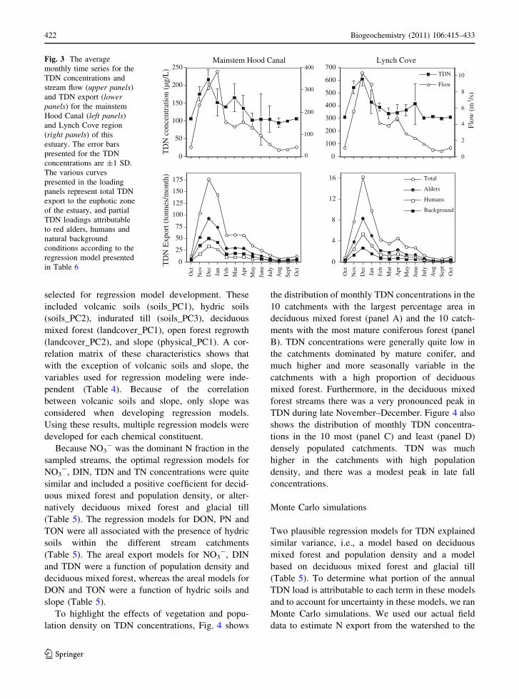
Due to the combined effect of two-fold higher

TDN concentrations which peaked in December, and

eight-fold higher flows which peaked in January,

greater than 60% of TDN export from this watershed

to the mainstem Hood Canal and Lynch Cove

occured during the 3 months of November–January

(Fig. 3). Conversely, only 15% of TDN export from

the watershed occurred during the 5 month period

from June to October. The annual TDN time series

0

100

200

300

400

500

Nitr

ogen

con

c. (

µg/L

)

2 4 6 8

10

Oly. Mtns

tcObeF AugJuneApr

0

100

200

300

400

500

Nitr

ogen

con

c. (

µg/L

)

018642

Lowlands

Particulate N

DON

Ammonium

Nitrate

(A) Lowland Tributaries

(B) Olympic Mtn. Tributaries

Fig. 2 Two-year average concentrations of PN, NH4?, DON,

and NO2- ? NO3

- observed in a lowland streams (32

streams), and b Olympic Mountain watersheds (Big Quilcene,

Dosewallips, Duckabush, Hamma Hamma, Little Quilcene)


123

http://www.hoodcanal.washington.edu

http://www.hoodcanal.washington.edu

shows concentrations increased dramatically during

November and December as flow increased, but that

TDN concentrations dropped off markedly in January

even as flow continued to increase (Fig. 3). A similar

pattern was observed in Lynch Cove, although in that

region flow peaked in December.

Statistical models of watershed effects

on nutrients

The normalized coefficient loadings for the three

separate principal component analyses (i.e., soils,

vegetation type, and watershed physical characteris-

tics) are shown in Table 3. The soils data matrix was

reduced to three principal components that together

explained 79% of the soils variance (Table 3). The

soil variables most strongly correlated with soils_PC1

were volcanic and spodosol soils, and rock outcrops.

The soil types highly correlated with soils_PC2 were

hydric, histic/histosol and wetland soils, as well as soil

water capacity. Soils_PC3 was highly positively

correlated with weakly developed soils not derived

from glacial till (e.g., entisols and inceptisols), and

highly negatively correlated with glacially indurated

(till) soils. Two land cover principal components

explained 50 and 31%, respectively, of the total land

cover variance. Landcover_PC1 was highly positively

correlated with deciduous mixed forest and negatively

correlated with mature coniferous forest. Landcov-

er_PC2 was strongly correlated with open forest/

regrowth, which comprised 9% of the watershed. The

watershed physical characteristics matrix was reduced

to a single principal component that explained 85% of

the total variance (Table 3). The four physical char-

acteristics were highly collinear and had similar

strong coefficient loadings on physical_PC1.

Based on these PCA results, six watershed char-

acteristics, as well as population density, were

Table 2 Regional flow-weighted mean nitrogen concentrations, annual loading rates, and area-normalized loading rates based on the

2005–2006 monthly grab samples

NO3 NH4 NO2 DON PN DIN TDN TON TN

Flow-weighted mean concentrations (lg l-1)

N Fork Skokomish diversion 22 10.0 0.4 38 36 33 72 75 108

Skokomish River 71 9.5 2.9 22 81 83 106 103 186

Other Olympic Mountain rivers 61 7.6 0.4 38 34 69 108 72 142

Kitsap/lowland watersheds 198 12.7 0.9 72 37 212 283 108 319

Unsampled Kitsap/lowland watershedsa 325 12.7 1.0 114 43 339 452 157 495

Overall flow-weighted concentration 97 9.5 1.2 44 49 108 152 93 201

Loads (MT year-1)

N Fork Skokomish diversion 14 6.2 0.23 24 22 20 44 46 67

Skokomish River 95 12.8 3.95 30 109 111 141 139 250

Other Olympic Mountain rivers 109 13.5 0.63 68 60 124 192 128 252

Kitsap/lowland watersheds 86 5.5 0.37 31 16 92 122 47 138

Unsampled Kitsap/lowland watershedsa 144 5.6 0.42 50 19 150 199 69 218

Total annual load 447 44 5.6 202 226 496 699 429 925

Percentage of total load (%) 48 5 1 22 24

Loading rates (kg year-1 ha-1)

N Fork Skokomish diversion 0.5 0.24 0.01 0.9 0.9 0.8 1.7 1.8 2.6

Skokomish River 2.8 0.38 0.12 0.9 3.2 3.3 4.2 4.1 7.5

Other Olympic Mountain rivers 1.1 0.14 0.01 0.7 0.6 1.3 1.9 1.3 2.6

Kitsap/lowland watersheds 1.5 0.10 0.01 0.5 0.3 1.6 2.1 0.8 2.4

Unsampled Kitsap/lowland watershedsa 2.3 0.09 0.01 0.8 0.3 2.4 3.2 1.1 3.5

Whole watershed loading rates 1.8 0.15 0.02 0.7 0.8 2.0 2.7 1.5 3.3

a Concentrations shown for Unsampled Kitsap/lowland watersheds are based on monthly averages of those from the four most

populated catchments in the region (Big Beef, Seabeck, Tahuya, Union)


123

selected for regression model development. These

included volcanic soils (soils_PC1), hydric soils

(soils_PC2), indurated till (soils_PC3), deciduous

mixed forest (landcover_PC1), open forest regrowth

(landcover_PC2), and slope (physical_PC1). A cor-

relation matrix of these characteristics shows that

with the exception of volcanic soils and slope, the

variables used for regression modeling were inde-

pendent (Table 4). Because of the correlation

between volcanic soils and slope, only slope was

considered when developing regression models.

Using these results, multiple regression models were

developed for each chemical constituent.

Because NO3- was the dominant N fraction in the

sampled streams, the optimal regression models for

NO3-, DIN, TDN and TN concentrations were quite

similar and included a positive coefficient for decid-

uous mixed forest and population density, or alter-

natively deciduous mixed forest and glacial till

(Table 5). The regression models for DON, PN and

TON were all associated with the presence of hydric

soils within the different stream catchments

(Table 5). The areal export models for NO3-, DIN

and TDN were a function of population density and

deciduous mixed forest, whereas the areal models for

DON and TON were a function of hydric soils and

slope (Table 5).

To highlight the effects of vegetation and popu-

lation density on TDN concentrations, Fig. 4 shows

the distribution of monthly TDN concentrations in the

10 catchments with the largest percentage area in

deciduous mixed forest (panel A) and the 10 catch-

ments with the most mature coniferous forest (panel

B). TDN concentrations were generally quite low in

the catchments dominated by mature conifer, and

much higher and more seasonally variable in the

catchments with a high proportion of deciduous

mixed forest. Furthermore, in the deciduous mixed

forest streams there was a very pronounced peak in

TDN during late November–December. Figure 4 also

shows the distribution of monthly TDN concentra-

tions in the 10 most (panel C) and least (panel D)

densely populated catchments. TDN was much

higher in the catchments with high population

density, and there was a modest peak in late fall

concentrations.

Monte Carlo simulations

Two plausible regression models for TDN explained

similar variance, i.e., a model based on deciduous

mixed forest and population density and a model

based on deciduous mixed forest and glacial till

(Table 5). To determine what portion of the annual

TDN load is attributable to each term in these models

and to account for uncertainty in these models, we ran

Monte Carlo simulations. We used our actual field

data to estimate N export from the watershed to the

0

100

200

300

400

0

50

100

150

200

250

TD

N c

once

ntra

tion

(µg/

L)

Oct

Nov D

ec

Jan

Feb

Mar

Apr

May

June

July

Aug

Sep

t

Oct

Mainstem Hood Canal

0

25

50

75

100

125

150

175

TD

N E

xpor

t (to

nnes

/mon

th)

Oct

Nov

Dec

Jan

Feb

Mar

Apr

May

June

July

Aug

Sept

Oct

0

2

4

6

8

10

Flow

(m

3 /s)

0

100

200

300

400

500

600

700

Oct

Nov D

ec

Jan

Feb

Mar

Apr

May

June

July

Aug

Sep

t

Oct

Lynch Cove

Flow

TDN

0

4

8

12

16

Oct

Nov

Dec

Jan

Feb

Mar

Apr

May

June

July

Aug

Sept

Oct

Background

Humans

Alders

Total

Fig. 3 The average

monthly time series for the

TDN concentrations and

stream flow (upper panels)

and TDN export (lowerpanels) for the mainstem

Hood Canal (left panels)

and Lynch Cove region

(right panels) of this

estuary. The error bars

presented for the TDN

concentrations are ±1 SD.

The various curves

presented in the loading

panels represent total TDN

export to the euphotic zone

of the estuary, and partial

TDN loadings attributable

to red alders, humans and

natural background

conditions according to the

regression model presented

in Table 6


123

Table 3 The partial coefficient loadings (as r values) for the soils, land cover, and physical characteristics principal component

analyses

Soil types and characteristics PCA % Hood Canal

watershed in each

soil type

Soils_PC1 Soils_PC2 Soils_PC3

Percent of variation explained within PCA 34.3 28.7 15.6

Percent area with weakly developed soils (entisols excluding till) 41 -0.26 -0.09 0.89

Log(percent catchment area with volcanic soils) 33 0.95 -0.03 0.19

Percent catchment area with till soil 18 -0.43 0.06 -0.85

Log(percent catchment area in rock outcrops) 12 0.91 -0.17 -0.03

Log(percent catchment area in riverwash/water) 4.9 0.37 0.60 0.06

Log(percent catchment area with hydric soils) 2.8 -0.02 0.93 -0.17

Log(percent catchment area in spodosol soils) 2.5 0.78 -0.26 -0.14

Log(percent catchment area with wetland mineral soils) 2.3 0.01 0.88 -0.21

Log(percent catchment area with histosols/histic soils) 0.6 -0.03 0.88 0.22

Depth-integrated soil organic matter – 0.53 0.55 0.37

Depth-integrated soil cation exchange capacity – -0.73 -0.26 0.48

Depth-integrated soil water capacity – -0.13 0.81 -0.10

Soil bulk density (36–60 inches below surface) – -0.91 -0.28 0.02

Depth averaged percent clay (mean) – 0.66 0.19 0.34

Land cover types PCA Watershed in each

land cover type (%)

LC_PC1 LC_PC2

Percent of variation explained within PCA 50.1 30.5

Mature coniferous forest 49 -0.80 -0.59

Deciduous/mixed forest 10 0.96 -0.08

Grass/shrubs/crops/early regrowth 7.9 0.42 0.38

Young coniferous forest 7.9 0.42 0.21

Sub-alpine forest 5.9 -0.34 -0.14

Open forest/regrowth 5.2 0.09 -0.92

Marsh/wetland/shoreline/shallow water 5.1 -0.11 0.10

Snow/ice 2.8 -0.32 -0.14

Bare ground/clearcut 2.7 -0.08 -0.04

Water 1.8 -0.09 0.00

Low density urban 1.0 0.22 0.22

Cloud 0.7 -0.05 -0.26

High density urban 0.2 0.08 0.26

Cloud shadow 0.1 0.34 -0.20

Physical characteristics PCA Physical_PC1

Percent of variation explained within PCA 84.9

Log(watershed area) 0.82

Log(elevation) 0.86

Mean slope (%) 0.81

Log(mean annual flow 2005–2006) 0.90

The soils, land cover and physical characteristics most strongly associated with a particular PC are indicated in bold


123

Hood Canal estuary, and the Monte Carlo simulations

based on our regression models to apportion this

loading between the putative sources identified in our

statistical analyses. For example, our most probable

TDN model is TDN concentration (lg l-1) in any

stream = DMF 9 9.3 ? pop density 9 3.5 ? 61

(Table 5). For a hypothetical stream with average

attributes for all streams (i.e., 16 people km2 and

14% DMF) and an overall observed TDN export of

20 MT, our regression model would predict

61 lg TDN l-1 is naturally occurring (3.5 9

16 =) 56 lg l-1 is associated with humans, and

Table 4 Correlation matrix on the variables originally selected for multiple regression

Volcanic

soils

Log(hydric

soils)

Till Deciduous

mixed forest

Open forest

regrowth

Slope

Log(hydric soils) -0.12

Till -0.52 0.18

Deciduous mixed forest -0.28 0.56 0.28

Open forest regrowth -0.32 -0.03 0.11 0.11

Slope 0.90 -0.32 -0.43 -0.45 -0.27

Population density -0.43 0.17 0.47 0.18 0.00 -0.41

Volcanic soils were removed from the regression independent variable matrix after finding this term was highly correlated with slope

Table 5 The significant

multiple regression

equations for the various

nitrogen species with AIC

weight [10%

Terms with the lowest

p values are listed first

Hydric soils and deciduous

mixed forest were

expressed as watershed area

percentages (numbers

between zero and 100).

Population density was

expressed as people km-2,

and slope was

dimensionless

AIC

weight

R2

Concentration (lg l-1)

NO3 = 7.46 9 (deciduous mixed forest) ? 3.37 9 (pop density) ? 23.8 0.49 0.42

NO3 = 1.95 9 (till) ? 6.90 9 (deciduous mixed forest) ? 0.608 0.47 0.42

DIN = 7.25 9 (deciduous mixed forest) ? 3.46 9 (pop density) ? 42.6 0.63 0.40

DIN = 1.83 9 (till) ? 6.81 9 (deciduous mixed forest) ? 24.1 0.31 0.38

TDN = 9.34 9 (deciduous mixed forest) ? 3.47 9 (pop density) ? 60.9 0.48 0.46

TDN = 2.01 9 (till) ? 8.77 9 (deciduous mixed forest) ? 37.2 0.46 0.45

DON = 33.4 9 log(hydric soils) ? 22.1 0.94 0.35

PN = 11.6 9 log(hydric soils) ? 28.3 0.98 0.30

TON = 35.2 9 log(hydric soils) ? 1.30 9 (deciduous mixed forest) ? 38.0 0.77 0.53

TON = 45.0 9 log(hydric soils) ? 50.4 0.23 0.48

TN = 9.94 9 (deciduous mixed forest) ? 3.57 9 (pop density) ? 88.6 0.51 0.47

TN = 2.02 9 (till) ? 9.38 9 (deciduous mixed forest) ? 65.4 0.42 0.46

Areal loading (kg ha-1 year-1)

NO3 = 0.0265 9 (deciduous mixed forest) ? 0.0235 9 (pop

density) ? 0.728

0.71 0.27

NO3 = 0.0267 9 (pop density) ? 1.12 0.21 0.19

DIN = 0.0260 9 (pop density) ? 1.28 0.87 0.17

DIN = 0.0289 9 (deciduous mixed forest) ? 1.20 0.13 0.09

TDN = 0.0251 9 (pop density) ? 1.75 0.75 0.15

TDN = 0.0313 9 (deciduous mixed forest) ? 1.62 0.25 0.10

DON = 0.179 9 log(hydric soils) ? 0.0110 9 (slope) ? 0.0414 0.99 0.41

PN = 0.0104 9 (slope) ? 0.191 1.00 0.14

TON = 0.320 9 log(hydric soils) ? 0.0239 9 (slope) ? 0.0452 0.99 0.42


123

(9.3 9 14 =) 102 lg l-1 is associated with DMF. In

relative terms, these values equate to 28, 26 and 47%

of the TDN coming from natural sources, humans and

deciduous vegetation, respectively. When adjusted

for the observed load, this suggests 5.6, 5.1 and

9.5 MT, respectively, of TDN in this hypothetical

stream originated from the three sources indicated

above. When also taking into account uncertainty

associated with the coefficients of the multiple

regression model, the Monte Carlo simulations for

both models predicted deciduous mixed forest was

associated with 51 ± 15% of the annual TDN load to

Hood Canal (Table 6), or 354 ± 202 MT year-1.

The same simulations suggested 13.6 ± 6.5% of the

annual TDN load was associated with population

density (Table 6), or 95 ± 45 MT year-1. These

Monte Carlo simulations were also run for just Lynch

Cove, and for this region 56 ± 11% of the TDN load

could be attributed to deciduous mixed forest, and

31 ± 10% was associated with population density

(Table 6).

Box model of N inputs to Hood Canal and Lynch

Cove

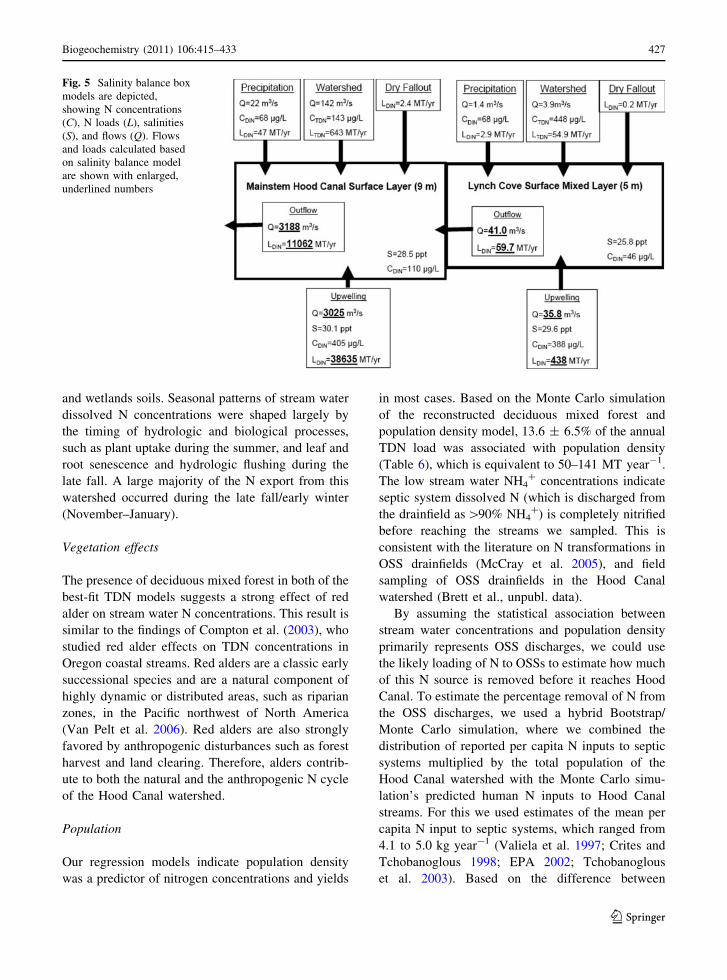
The surface mixed layer salinities were only slightly

lower than salinities at depth, so in both Hood Canal

and Lynch Cove, the calculated the upwelling flows

were much larger than freshwater inflows to the

euphotic zone (Fig. 5). Similarly, upwelling was the

major N source to the surface mixed layer, where it

constituted 88% and 98% of the N load to the

euphotic zone of Lynch Cove and the mainstem Hood

Canal, respectively. Upwelling was a larger propor-

tion of the N load to the surface layer of the mainstem

Hood Canal because the relative difference between

salinities at the surface and at depth is smaller in the

mainstem Hood Canal, and the watershed N concen-

tration is lower for the mainstem Hood Canal

(143 lg TDN l-1) than for the Lynch Cove tributar-

ies (448 lg TN l-1). In both Lynch Cove and the

mainstem Hood Canal, the N concentration of

upwelling water was high (388 and 405 lg TDN l-1,

0

200

400

600

800

1000

TD

N c

once

ntra

tion

(µg/

L)

Jan

Feb

Mar

Apr

May Jun

July

Aug

Sep

t

Oct

Nov

DecJan

Feb

Mar

Apr

May Jun

July

Aug

Sep

t

Oct

Nov

Dec

0

200

400

600

800

1000

TD

N c

once

ntra

tion

(µg/

L)

(A) (B)

(C) (D)

Fig. 4 a Average monthly

TDN concentrations in the

ten catchments with the

highest proportion

deciduous mixed forest

(using the site codes

provided in Fig. 1, these

streams are 1, 2, 3, 22, 31,

32, 37, 41, 42 and 43).

b TDN concentrations in

the ten catchments with the

most mature coniferous

forest (i.e., 4, 7, 8, 10, 11,

12, 13, 27, 28 and 36).

c Average TDN

concentrations in the 10

most densely populated

catchments (i.e., 24, 25, 28,

32, 33, 34, 35, 41, 42 and

43). d TDN concentrations

in the 10 least densely

populated catchments (i.e.,

1, 5, 6, 7, 8, 9, 12, 13, 19

and 20)


123

respectively). A sensitivity analysis showed estimates

of the upwelling flow and the related marine N

loading calculations depended to some extent on the

choice of the surface depth assumed in the Hood

Canal box model. Reducing the assumed pycnocline

depth from 9 to 7 m decreased the estimated

upwelling flow by 1%, whereas increasing the

assumed pycnocline to 11 m increased the estimated

upwelling flow by 24%. The direct rainwater N load

to the surface of Hood Canal was relatively small

because the watershed area is much larger than the

estuary’s surface, and the rainwater DIN concentra-

tion was low (68 DIN lg l-1) (Fig. 5). However,

across the entire watershed rainwater DIN was more

than sufficient to account for the baseline stream-

water DIN concentrations (i.e., &70 lg l-1).

Discussion

Terrestrial controls on stream N export

Watershed nitrogen export to Hood Canal was

strongly correlated with deciduous mixed forest and

population density. High dissolved N concentrations

were to a lesser extent statistically associated with the

presence of glacial till, while organic N export was

higher in catchments with a high prevalence of hydric

Table 6 Models for TDN concentration reconstructed from original variables and analyzed in a Monte Carlo simulation

Reconstructed models (with coefficient standard deviations)

TDN (lg l-1) = 2.0 (±0.8) 9 Till ? 8.8 (±2.1) 9 Mixed deciduous forest ? 37.2 (±48.6)

TDN (lg l-1) = 3.5 (±1.4) 9 Population density ? 9.4 (±2.0) 9 Mixed deciduous forest ? 60.9 (±44.7)

Percentage (±1 SD)

of TDN load attributed

to each term

Monte Carlo simulation results for Hood Canala

Mixed deciduous forest/till model

Mixed deciduous forest 51.0 (±14.5)

Till 25.1 (±10.3)

Intercept (background) 23.8 (±18.0)

Mixed deciduous forest/population density model

Mixed deciduous forest 50 9 (±14 8)

Population density 13.6 (±6.5)


Monte Carlo simulation results for Lynch Covea

Mixed deciduous forest/till model


Till 27.1 (±9.7)


Mixed deciduous forest/population density model


Population density 30.9 (±10.2)


a A total of four Monte Carlo simulations were run by applying each of the two models to the 43 sampled catchments and to the

unsampled area of Hood Canal and then by applying each model to the 12 catchments and unsampled area draining to Lynch Cove. Based

on the intercepts and coefficients and their standard deviations, a random normal distribution (n = 50,000) was created term in each

model. These distributions were applied to the observed catchment characteristics (i.e. vegetation, population density, and soil type) to

predict the expected contribution of each model component to TDN concentrations in each catchment. All terms were constrained to be

positive so that negative predicted concentrations could be avoided. These values were then multiplied by the observed average annual

flow from each catchment and summed for the entire Hood Canal watershed (or Lynch Cove watershed) to derive 50,000 estimates of the

partial contributions of vegetation, population density, and glacial till to terrestrial TDN export to the Hood Canal


123

and wetlands soils. Seasonal patterns of stream water

dissolved N concentrations were shaped largely by

the timing of hydrologic and biological processes,

such as plant uptake during the summer, and leaf and

root senescence and hydrologic flushing during the

late fall. A large majority of the N export from this

watershed occurred during the late fall/early winter

(November–January).

Vegetation effects

The presence of deciduous mixed forest in both of the

best-fit TDN models suggests a strong effect of red

alder on stream water N concentrations. This result is

similar to the findings of Compton et al. (2003), who

studied red alder effects on TDN concentrations in

Oregon coastal streams. Red alders are a classic early

successional species and are a natural component of

highly dynamic or distributed areas, such as riparian

zones, in the Pacific northwest of North America

(Van Pelt et al. 2006). Red alders are also strongly

favored by anthropogenic disturbances such as forest

harvest and land clearing. Therefore, alders contrib-

ute to both the natural and the anthropogenic N cycle

of the Hood Canal watershed.

Population

Our regression models indicate population density

was a predictor of nitrogen concentrations and yields

in most cases. Based on the Monte Carlo simulation

of the reconstructed deciduous mixed forest and

population density model, 13.6 ± 6.5% of the annual

TDN load was associated with population density

(Table 6), which is equivalent to 50–141 MT year-1.

The low stream water NH4? concentrations indicate

septic system dissolved N (which is discharged from

the drainfield as [90% NH4?) is completely nitrified

before reaching the streams we sampled. This is

consistent with the literature on N transformations in

OSS drainfields (McCray et al. 2005), and field

sampling of OSS drainfields in the Hood Canal

watershed (Brett et al., unpubl. data).

By assuming the statistical association between

stream water concentrations and population density

primarily represents OSS discharges, we could use

the likely loading of N to OSSs to estimate how much

of this N source is removed before it reaches Hood

Canal. To estimate the percentage removal of N from

the OSS discharges, we used a hybrid Bootstrap/

Monte Carlo simulation, where we combined the

distribution of reported per capita N inputs to septic

systems multiplied by the total population of the

Hood Canal watershed with the Monte Carlo simu-

lation’s predicted human N inputs to Hood Canal

streams. For this we used estimates of the mean per

capita N input to septic systems, which ranged from

4.1 to 5.0 kg year-1 (Valiela et al. 1997; Crites and

Tchobanoglous 1998; EPA 2002; Tchobanoglous

et al. 2003). Based on the difference between

Fig. 5 Salinity balance box

models are depicted,

showing N concentrations

(C), N loads (L), salinities

(S), and flows (Q). Flows

and loads calculated based

on salinity balance model

are shown with enlarged,

underlined numbers


123

probable N input to septic systems and the N output

to streams from this source suggested by our models,

we calculated 56 ± 20% of the N loaded to OSSs

was removed by denitrification in subsurface flows

prior to reaching the Hood Canal. However, N

removal from OSS effluents in areas we have not

sampled may be lower than in areas we have sampled

because much of the population lives in very close

proximity (i.e., \50 m) to the marine shoreline and

subsurface flow distances to surface water in these

areas are much shorter than in the sampled catch-

ments. Thus, the assumption that the unsampled

areas’ N concentrations and yields are similar to

those of the most populated sampled catchments

should be supported by further field sampling.

Soils

Shallow water tables maximize the exposure of

groundwater to soil C, and are often associated with

enhanced denitrification (Hedin et al. 1998; Hill

1996). However, in this study the presence of a

compacted glacial till layer was positively correlated

with stream water TDN concentrations. Although the

reasons for this correlation cannot be determined

from the current study, we speculate the cause may be

shallow routing through soils which could short-

circuit the groundwater removal processes where

most denitrification probably occurs in the coarse-

textured soils of this watershed.

Hydric, histic and wetland soils occurred in the

best-fit DON and TON models. Higher dissolved

organic matter concentrations due to riparian wet-

lands have been found in several other studies (e.g.,

Wetzel 1992; Gergel et al. 1999). The effect of

wetland soils on organic N is most obvious in the

catchment with the largest percentage of its area in

wetland/organic soils. In this catchment (Skabob

Creek) TON was 92% of TN, while in the other

catchments TON averaged 46% of TN. These rela-

tionships are similar to those observed in a survey of

TON yields in 850 streams across the conterminous

US (Scott et al. 2007).

Biological versus physical drivers

Co-occurrence of seasonal senescence of deciduous

vegetation and the onset of autumn rains makes it

difficult to distinguish between biological and

physical drivers of N flushing (Bechtold et al.

2003). Biological influences on N concentration can

be inferred from large differences between the

seasonal cycles of TDN concentrations in catchments

with high and low proportions of deciduous mixed

forest (Fig. 4). In catchments with high population

density, average concentrations were high but sea-

sonal cycles were more muted (Fig. 4). In order to

better differentiate influences on the seasonal

responses for these two stream types, we separated

our entire dataset into streams with above and below

median proportions of deciduous mixed forest and

population density. This isolated six catchments with

high population density/low deciduous mixed forest,

and five streams with low population density/high

deciduous mixed forest. These two sets of streams

had nearly identical average annual TDN concentra-

tions (i.e., &420

lg l-1), but the high deciduous mixed forest streams

had substantially more variation between annual

minimum and maximum values (i.e., 252–859

lg l-1, respectively) than did the high population

density streams (i.e., 375 and 561 lg l-1, respec-

tively). This suggests OSS discharges impart a higher

baseline TDN concentration, but less seasonal vari-

ation than does N export associated with red alders.

The importance of hydrology is suggested by the

positive correlation between TDN concentrations and

monthly mean flow (r = 0.49). In both years, the

highest TDN concentrations were in the early part of

the wet season (November and December), indicating

that by the second half of the wet season (January to

February) soil labile N had been largely flushed out

of the soils. Our findings parallel those of other

studies from Ontario and Washington State’s Olym-

pic Peninsula, which showed the importance of

hydrologic flushing as a control on N discharge

(Creed et al. 1996; Bechtold et al. 2003).

At global (e.g., Caraco and Cole 1999) and

continental (e.g., Scott et al. 2007) scales, runoff is

a good predictor of terrestrial N yield, leading some

to conclude that high discharges lead to less process-

ing and removal of anthropogenic and atmospheric N

loads and therefore greater streamwater N yields

(Jaworski et al. 1992). In general we have not found

this to be the case in the Hood Canal watershed.

Among the 43 catchments’ 2 year mean TDN yields,

areal runoff was not correlated with areal TDN yield

(r = 0.19, p = 0.23). One exception is the


123

Skokomish River, which had the highest runoff rate

and a high N yield despite low N concentrations

(Table 2). Several studies have found inter-annual

variations in N load are of the same scale (Salvia-

Castellvi et al. 2005) or greater than (Riggan et al.

1985; Jaworski et al. 1992) inter-annual variations in

discharge. In contrast, we found that total TDN

export to the Hood Canal estuary was almost

identical between dry and wet years when stream-

flows differed by 29%. These results suggest that

there was a steady amount of dissolved N available to

be leached on an annual basis, and greater precipi-

tation did not increase watershed TDN yield.

A box model of watershed TDN contributions to Hood

Canal

Terrestrial N loading to the surface layer (i.e., the

euphotic zone) was more important in Lynch Cove,

where it accounted for 11.1% of total N load, than in the

mainstem Hood Canal, where it only accounted for

1.6% of the N load (Fig. 5). Part of this difference can

be attributed to higher TDN concentrations in

watershed inputs to Lynch Cove (448 lg l-1) than

the mainstem Hood Canal (143 lg l-1). Further, the

surface salinity of Lynch Cove (25.7 ppt) was

substantially lower than that of the mainstem Hood

Canal (28.5 ppt), which indicates Lynch Cove received

proportionally more riverine and groundwater inputs.

To estimate what portion of the load to Lynch Cove

was due to anthropogenic sources, we repeated the

deciduous mixed forest and population density Monte

Carlo simulation while only using tributaries and

groundwater inputs to Lynch Cove (Table 6). This

showed 52 ± 11% of the terrestrial N export was

associated with deciduous mixed forest and 31 ± 10%

of the watershed load was associated with population

density. Combining this model with the salinity

balance showed 5.8 ± 1.2 and 3.4 ± 1.1%, respec-

tively, of the overall N load to the Lynch Cove surface

mixed layer can be statistically associated with indirect

(i.e., red alder) and direct (OSS discharges) anthropo-

genic inputs. In both Lynch Cove and the mainstem

Hood Canal, direct DIN inputs to the surface of the

estuary via rainwater and dry fallout were very minor

sources. However, because NADP data for the western

Washington State region indicate rainwater DIN

concentrations were &70 lg l-1 (NADP 2008), and

the overall watershed average TDN concentration was

152 lg l-1, atmospheric loading cannot be dismissed

as an insignificant N source to the actual watershed. It is

also noteworthy that these rainwater DIN concentra-

tions were a factor &20 less than what is commonly

encountered in the eastern seaboard of the United

States where rainwater DIN concentrations range

between 500 and 2,500 lg l-1 (Whitall et al. 2003;

Kelly et al. 2009). Low rainwater DIN concentrations

may also be one of the reasons why streams and rivers

draining to Hood Canal have much lower DIN

concentrations (213 ± 208 lg l-1) than do streams

draining to Lake Washington (875 ± 324 lg l-1) in

the metropolitan Seattle area only 40–70 km to the

west (Brett et al. 2005).

The salinity mass balance model also allowed us to

estimate the mean hydraulic residence time (HRT) of

the surface mixed layer. For the mainstem Hood Canal

the estimated steady state HRT was 12 days. This short

HRT indicates much of the wet season watershed TDN

load should be advected out of the estuary before the

peak phytoplankton growing season in late spring and

summer (HCDOP 2008). However, it is notable that

during the uncommonly dry February weather in both

2005 and 2006, phytoplankton N uptake reduced DIN

in the surface mixed layer to\10 lg l-1. This suggests

that although the most important watershed N loads for

promoting phytoplankton productivity are those that

occur during the peak phytoplankton months in the

spring and summer, watershed N export during

November–January could be important during sunny

(i.e., high algal productivity) periods during the winter.

During the spring and summer peak phytoplankton

growth, the TDN load associated with humans may be

especially important, since population density and

OSS effluents are associated with a higher baseline N

concentration and less seasonal variability. Thus,

during low flow months, population density may

contribute a higher proportion of the N load to Lynch

Cove than indicated by the 3.4% estimate above.

In this study we have placed the greatest emphasis

on TDN loading to Hood Canal because TDN is

representative of the N which stimulates phytoplank-

ton production, and it is this phytoplankton produc-

tion which exerts an oxygen demand in the bottom

waters of the estuary as senescent cells or zooplank-

ton fecal pellets settle to the sediments. Field research

on Hood Canal has shown that during the peak

phytoplankton growth period of April to October,

DIN concentrations in the surface layer are drawn


123

down to very low levels (i.e., \10 lg l-1) (HCDOP

2008). This indicates that nearly all of the N loaded to

the euphotic zone during this time of year is taken up

by phytoplankton and used to generate new growth.

Due to the Redfield ratio of marine phytoplankton

(i.e., C:N molar ratio &7) and the stoichiometry of

nitrification, the complete oxidation of 1 mol of

phytoplankton biomass requires approximately 9 mol

of oxygen (O2). Thus during peak phytoplankton

growth periods each mole of TDN loaded from

watershed sources to the euphotic zone of Hood

Canal will consume approximately 21 times its mass

in dissolved oxygen when it decomposes.

Based on the salinity mass balance values pre-

sented above, it is unlikely that watershed TDN

export (and in particular that TDN associated with

anthropogenic activities) will result in a substantial

additional oxygen debt in the mainstem Hood Canal

because the watershed only contributed 2% of the N

loading to the surface layer of overall estuary. Our

salinity mass balance calculations indicate the load-

ing of marine derived TDN to the surface layer of the

mainstem Hood Canal is 39,000 MT year-1 (Fig. 5).

As previously noted, this estimate is high (relative to

terrestrial loading) because the salinity data indicate

the surface layer of this estuary is 95% marine and

the marine water entrained into the surface layer has

nearly three times the nitrogen content of freshwater

inputs (Fig. 5). Our 39,000 MT year-1 marine con-

tribution estimate agrees moderately well with Paul-

son et al.’s (2006) 10,100–34,000 MT year-1

estimate. Paulson et al.’s estimate assumed similar

marine upwelling TDN concentrations, but calculated

the flux of marine water into Hood Canal based on

the net flow of currents into this estuary. If we assume

a population of 45,300 individuals (Table 1) each

contributing 4.5 ± 0.5 kg N year-1 to the estuary

with zero N removal, we can consider a worst case

scenario for N inputs to this estuary. In this

hypothetical case, the flux of OSS N would be

equivalent to 29 ± 4% of watershed export to Hood

Canal, but only 0.5 ± 0.1% of marine loading.

In the Lynch Cove sub-basin inferring the magni-

tude of anthropogenic N inputs is complicated by the

fact that our stream monitoring program does not

capture the immediate shoreline areas were most

water flows directly to the estuary via subsurface flow

paths, and where many people reside. We have

accounted for these ‘‘unsampled inputs’’ in our

watershed nitrogen budget by applying the same

areal hydrologic yields and runoff TDN concentra-

tions as observed in several densely populated

catchments that were sampled (see Tables 1, 2).

Our statistical approach estimates total watershed

export contributes 11% of nitrogen loading to the

euphotic zone of Lynch Cove, and most of this

nitrogen was statistically associated with indirect (red

alder) and direct (OSS) anthropogenic N sources, i.e.,

5.8 ± 1.2 and 3.5 ± 1.1% of total loading, respec-

tively. If we consider a worst-case-scenario for OSS

N inputs to Lynch Cove from the unsampled

shoreline areas, i.e., 4,500–5,000 people (HCDOP,

unpublished data) times 4–5 kg N year-1, then it is

conceivable that an additional 21 ± 3 MT year-1

could come from this source which would amount to

an additional 4 ± 1% of total loading.

While estuarine hypoxia can have natural causes,

it is often the result of anthropogenic nutrient sources

(Diaz and Rosenberg 2008). Several classic case

studies of eastern North American estuaries have

concluded human wastewaters and agricultural runoff

played major or even the main role in worsening

hypoxia, e.g., Waquoit Bay in Massachusetts (Valiela

et al. 1997), Narragansett Bay in Rhode Island (Nixon

1997), Chesapeake Bay in Maryland/Virginia (Kemp

et al. 2005) and the Neuse River Estuary in North

Carolina (Paerl 2006). Hood Canal differs from these

better known systems in that its watershed is much

less densely populated and its estuarine circulation is

very dominated by marine inflows with quite high

DIN concentrations (Mackas and Harrison 1997)

compared to the low marine DIN concentrations of

the mid-Atlantic shelf (Dafner et al. 2007). Further-

more, the DO dynamics of Hood Canal may have

been influenced by recent strong incursions of low

DO water onto the continental shelf off of the Pacific

Northwest of North America (Chan et al. 2008;

Connolly et al. 2010).

Conclusions

We present two multiple regression models to predict

TDN concentration in streams of the Hood Canal

watershed (R2 & 0.50). Both models show strong

effects of deciduous mixed forest (ca. 50%, red alder)

and suggest 51 ± 15% of the annual TDN load from

the watershed can be attributed to deciduous mixed


123

forest. One model includes population density as a

factor and suggests direct anthropogenic N inputs

(septic system effluents) contribute between 7.1 and

20.1% of the annual watershed TDN load to Hood

Canal. In the Lynch Cove area our data indicate

humans directly contributed 21 to 41% of the

terrestrial N export. A salinity balance model indi-

cated &98% of N loading to the surface layer of the

mainstem Hood Canal is from marine upwelling.

However, our calculations suggest watershed export

accounts for 11% of the total N load to Lynch Cove’s

surface mixed layer. Overall our results suggest OSS

N discharges are not an important contributor to

hypoxia in the mainstem Hood Canal, but this source

may contribute to oxygen depletion with the Lynch

Cove sub-basin.

Acknowledgments Funding was provided by the Hood

Canal Dissolved Oxygen Program through a Naval Sea

Systems Command Contract #N00024-02-D-6602 Task 50.

This study was also supported by funding from the Puget

Sound Regional Synthesis Model. Special thanks go to the

many persons and groups who collected field samples and

maintained stream flow gages for this project including:

EnviroVision, the Hood Canal Salmon Enhancement Group,

Jefferson Conservation District, Kitsap County Health District,

Mason Department of Environmental Health, and Skokomish

Tribe Natural Resources. We appreciate the constructive

comments by Mitsuhiro Kawase and Al Devol to earlier

drafts of this manuscript. We also thank Kathy Krogslund of

the Marine Chemistry Laboratory for processing the stream

chemistry samples, Amir Sheikh of PRISM for generating our

watershed figure, and Corinne Bassin of the Applied Physics

Laboratory for summarizing salinity data for Hood Canal.

References

Akaike H (1970) Statistical predictor identification. Ann Inst

Stat Math 22:203–217

Alberti M, Weeks R, Coe S (2004) Urban land cover change

analysis for the central Puget Sound: 1991–1999. J Pho-

togramm Eng Remote Sensing 70:1043–1052

Babson AL, Kawase A, MacCready P (2006) Seasonal and

interannual variability in the circulation of Puget Sound,

Washington: a box model study. Atmos Ocean 44:29–45

Bechtold JS, Edwards RT, Naiman RJ (2003) Biotic versus

hydrologic control over seasonal nitrate leaching in a

flood plain forest. Biogeochemistry 63:53–71

Binkley D, Cromack K, Baker DD (1994) Nitrogen fixation by

red alder: biology, rates and controls. In: Hibbs DE, De-

bell DS, Tarrant RF (eds) The biology and management of

red alder. Oregon State University Press, Corvallis,

pp 57–72

Boyer EW, Howarth RW, Galloway JN, Dentener FJ, Green

PA, Vorosmarty CJ (2006) Riverine nitrogen export from

the continents to the coasts. Glob Biogeochem Cycles

20:GB1S91

Brett MT, Arhonditsis GB, Mueller SE, Hartley DM, Frodge

JD, Funke DE (2005) Non-point source nutrient impacts

on stream nutrient and sediment concentrations along a

forest to urban gradient. Environ Manage 35:330–342

Burnham KP, Anderson DR (2002) Model selection and mul-

timodel inference: a practical information-theoretic

approach, 2nd edn. Springer-Verlag, New York

Busse LB, Gunkel G (2002) Riparian alder fens—source or

sink for nutrients and dissolved organic carbon? 2. Major

sources and sinks. Limnologica 32:44–53

Cairns MA, Lajtha K (2005) Effects of succession on nitrogen

export in the west-central Cascades, Oregon. Ecosystems

8:583–601

Caraco NF, Cole JJ (1999) Human impact on nitrate export: an

analysis using major world rivers. Ambio 28:167–170

Chan F, Barth JA, Lubchenco J, Kirincich A, Weeks H, Pet-

erson WT, Menge BA (2008) Novel emergence of anoxia

in the California Current System. Science 319:920

Clean Air Status and Trends Network (CASTNET) (2008) US

EPA air quality and deposition database. http://www.epa.

gov/castnet/. Cited 1 Feb 2008

Collias CE, McGary N, Barnes CA (1974) Atlas of physical

and chemical properties of Puget Sound and its approa-

ches. University of Washington Sea Grant Publication

WSG 74-1

Compton JE, Church MR, Larned ST, Hogsett WE (2003)

Nitrogen export from forested watersheds in the Oregon

Coast Range: the role of N2-fixing red alder. Ecosystems

6:773–785

Connolly TP, Hickey BM, Geier SL, Cochlan WP (2010)

Processes influencing seasonal hypoxia in the northern

California Current System. J Geophys Res 115:C03021

Creed IF, Band LE, Foster NW, Morrison IK, Nicolson JA,

Semkin RS, Jeffries DS (1996) Regulation of nitrate-N

release from temperate forests: a test of the N flushing

hypothesis. Water Resour Res 32:3337–3354

Crites R, Tchobanoglous G (1998) Small and decentralized

wastewater management systems. McGraw Hill Publish-

ing Company, Boston

Dafner EV, Mallin MA, Souza JJ, Wells HA, Parsons DC

(2007) Nitrogen and phosphorus species in the coastal and

shelf waters of Southeastern North Carolina, Mid-Atlantic

US coast. Mar Chem 103:289–303

Diaz RJ, Rosenberg R (2008) Spreading dead zones and con-

sequences for marine ecosystems. Science 321:926–929

Environmental Protection Agency (EPA) (2002) Onsite

wastewater treatment systems manual, EPA/625/R-00/

008. Environmental Protection Agency, Office of Water,

Office of Research and Development

Fenn ME, Poth MA, Aber JD, Baron JS, Bormann BT, Johnson

DW, Lemly AD, McNulty SG, Ryan DF, Stottlemyer R

(1998) Nitrogen excess in North American ecosystems:

predisposing factors, ecosystem responses, and manage-

ment strategies. Ecol Appl 8:706–733

Galloway JN, Dentener FJ, Capone DG, Boyer EW, Howarth

RW, Seitzinger SP, Asner GP, Cleveland CC, Green PA,

Holland EA, Karl DM, Michaels AF, Porter JH, Town-

send AR, Vorosmarty CJ (2004) Nitrogen cycles: past,

present, and future. Biogeochemistry 70:153–226


123

http://www.epa.gov/castnet/

http://www.epa.gov/castnet/

Gergel SE, Turner MG, Kratz TK (1999) Dissolved organic

carbon as an indicator of the scale of watershed influence

on lakes and rivers. Ecol Appl 9:1377–1390

Green PA, Vorosmarty CJ, Meybeck M, Galloway JN, Peter-

son BJ, Boyer EW (2004) Pre-industrial and contempo-

rary fluxes of nitrogen through rivers: a global assessment

based on typology. Biogeochemistry 68:71–105

Hedin LO, Armesto JJ, Johnson AH (1995) Patterns of nutrient

loss from unpolluted, old-growth temperate forests: eval-

uation of biogeochemical theory. Ecology 76:493–509

Hedin LO, von Fischer JC, Ostrom NE, Kennedy BP, Brown

MG, Robertson GP (1998) Thermodynamic constraints on

nitrogen transformations and other biogeochemical pro-

cesses at soil-stream interfaces. Ecology 79:684–703

Hill AR (1996) Nitrate removal in stream riparian zones.

J Environ Qual 25:743–755

Hood Canal Dissolved Oxygen Program (HCDOP) (2008)

Hood Canal water chemistry database. http://www.hood

canal.washington.edu/. Cited 1 Feb 2008

Howarth RW, Billen G, Swaney D, Townsend A, Jaworski N,

Lajtha K, Downing JA, Elmgren R, Caraco N, Jordan T,

Berendse F, Freney J, Kudeyarov V, Murdoch P, Zhu ZL

(1996) Regional nitrogen budgets and riverine N and P

fluxes for the drainages to the North Atlantic Ocean:

natural and human influences. Biogeochemistry 35:

75–139

Hurd TM, Raynal DJ (2004) Comparison of nitrogen solute

concentrations within alder (Alnus incana ssp. rugosa)

and non-alder dominated wetlands. Hydrol Process

18:2681–2697

Hurd TM, Raynal DJ, Schwintzer CR (2001) Symbiotic N2

fixation of Alnus incana ssp. rugosa in shrub wetlands of

the Adirondack Mountains, New York, USA. Oecologia

126:94–103

Imhoff ML, Tucker CJ, Lawrence WT, Stutzer DC (2000) The

use of multisource satellite and geospatial data to study the

effect of urbanization on primary productivity in the United

States. IEEE Trans Geosci Remote Sens 38:2549–2556

Jassby AD (1999) Uncovering mechanisms of interannual

variability from short ecological time series. In: Scow

KM, Fogg GE, Hinton DE, Johnson ML (eds) Integrated

assessment of ecosystem health. Lewis, Boca Raton,

pp 285–306

Jaworski NA, Groffman PM, Keller AA, Prager JC (1992) A

watershed nitrogen and phosphorus balance: the upper

Potomac River basin. Estuaries 15:83–95

Kelly VR, Weathers KC, Lovett GM, Likens GE (2009) Effect

of climate change between 1984 and 2007 on precipitation

chemistry at a site in northeastern USA. Environ Sci

Technol 43:3461–3466

Kemp WM, Boynton WR, Adolf JE, Boesch DF, Boicourt WC,

Brush G, Cornwell JC, Fisher TR, Glibert PM, Hagy JD,

Harding LW, Houde ED, Kimmel DG, Miller WD, Ne-

well RIE, Roman MR, Smith EM, Stevenson JC (2005)

Eutrophication of Chesapeake Bay: historical trends and

ecological interactions. Mar Ecol Prog Ser 303:1–29

Koh CN, Lee PF, Lin RS (2006) Bird species richness patterns

of northern Taiwan: primary productivity, human popu-

lation density, and habitat heterogeneity. Divers Distrib

12:546–554

Mackas DL, Harrison PJ (1997) Nitrogenous nutrient sources

and sinks in the Juan de Fuca Straight/Straight of Georgia/

Puget Sound estuarine system: assessing the potential for

eutrophication. Estuar Coast Shelf Sci 44:1–21

McCray JE, Kirkland SL, Siegrist RL, Thyne GD (2005)

Model parameters for simulating fate and transport of on-

site wastewater nutrients. Ground Water 43:628–639

NASA Landsat Program (2001) Landsat ETM? scene LE704

70272000212EDC00, Precision Geocorrection. USGS,

Sioux Falls, 07/30/2000

National Atmospheric Deposition Program (NADP) (2008)

Illinois State Water Survey. http://nadp.sws.uiuc.edu/.

Cited 1 Feb 2008

Newton JA, Thomson AL, Eisner LB, Hannach GA, Albertson

SL (1995) Dissolved oxygen concentrations in Hood

Canal: are conditions different than forty years ago? In:

Puget Sound research ‘95 proceedings, Puget Sound water

quality authority, Olympia

Nixon SW (1997) Prehistoric nutrient inputs and productivity

in Narragansett Bay. Estuaries 20:253–261

Paerl HW (2006) Assessing and managing nutrient-enhanced

eutrophication in estuarine and coastal waters: interactive

effects of human and climatic perturbations. Ecol Eng

26:40–54

Paerl HW, Dennis RL, Whitall DR (2002) Atmospheric

deposition of nitrogen: Implications for nutrient over-

enrichment of coastal waters. Estuaries 4B:677–693

Paulson AJ, Konrad CP, Frans LM, Noble MA, Kendall C,

Josberger EG, Huffman RL, Olsen TD (2006) Freshwater

and saline loads of dissolved inorganic nitrogen to Hood

Canal and Lynch Cove, western Washington. U.S. Geo-

logical Survey scientific investigations report 2006-5106,

91 pp

Perakis SS, Hedin LO (2002) Nitrogen loss from unpolluted

South American forests mainly via dissolved organic

compounds. Nature 418:416–419

Peterson DL, Schreiner EG, Buckingham NM (1997) Gradi-

ents, vegetation and climate: spatial and temporal

dynamics in the Olympic Mountains, USA. Glob Ecol

Biogeogr 6:7–17

Riggan PJ, Lockwood RN, Lopez EN (1985) Deposition and

processing of airborne nitrogen pollutants in Mediterra-

nean-type ecosystems of southern California. Environ Sci

Technol 19:781–789

Salvia-Castellvi M, Iffly JF, Borght PV, Hoffman L (2005)

Dissolved and particulate nutrient export from rural

catchments: a case study from Luxembourg. Sci Total

Environ 344:51–65

Scott D, Harvey J, Alexander R, Schwarz G (2007) Dominance

of organic nitrogen from headwater streams to large rivers

across the conterminous United States. Global Biogeo-

chem Cycles 21:GB1003

Soil Survey Geographic (SSURGO) Database (2006) Natural

Resources Conservation Service, United States Depart-

ment of Agriculture. http://soildatamart.nrcs.usda.gov.

Cited 15 Jun 2006

Sollins P, Grier CC, McCorison FM, Cromack K, Fogel R

(1980) The internal element cycles of an old growth

Douglas-fir ecosystem in western Oregon. Ecol Monogr

50:261–285


123

http://www.hoodcanal.washington.edu/

http://www.hoodcanal.washington.edu/

http://nadp.sws.uiuc.edu/

http://soildatamart.nrcs.usda.gov

Tchobanoglous G, Burton FL, Stensel HD (2003) Wastewater

engineering treatment and reuse. McGraw-Hill, Boston

Triska FJ, Sedell JR, Cromack K, Gregory SV, McCorison FM

(1984) Nitrogen budget for a small coniferous stream.

Ecol Monogr 54:119–140

Valiela I, Collins G, Kremer J, Lajtha K, Geist M, Seely B,

Brawley J, Sham CH (1997) Nitrogen loading from

coastal watersheds to receiving estuaries: new method and

application. Ecol Appl 7:358–380

Van Pelt R, O’Keefe TC, Latterell JJ, Naiman RJ (2006)

Riparian forest stand development along the Queets River

in Olympic National Park, Washington. Ecol Monogr

76:277–298

Vitousek PM, Aber JD, Howarth RW, Likens GE, Matson PA,

Schindler DW, Shlesinger WH, Tilman DG (1997)

Human alteration of the global nitrogen cycle: sources and

consequences. Ecol Appl 7:737–750

Wetzel RG (1992) Gradient-dominated ecosystems—sources

and regulatory functions of dissolved organic matter in

freshwater ecosystems. Hydrobiologia 229:181–198

Whitall D, Hendrickson B, Paerl H (2003) Importance of

atmospherically deposited nitrogen to the annual nitrogen

budget of the Neuse River estuary, North Carolina.

Environ Int 29:393–399

Younger PD, Kapustka LA (1983) N2(C2H2)ase activity by

Alnus incana ssp. rugosa (Betulaceae) in the northern

hardwood forest. Am J Bot 70:30–39


123

the inﬂuence of watershed characteristics on …. steinberg_etal_2011... · the inﬂuence of...

Documents