the interaction of labor markets and inflation: analysis...
TRANSCRIPT

1
The Interaction of Labor Markets and Inflation: Analysis of Micro Data from the International Wage
Flexibility Project
William T. Dickens, Lorenz Goette, Erica L. Groshen, Steinar Holden, Julian Messina, Mark E. Schweitzer, Jarkko Turunen, and Melanie Ward1
1 William Dickens is a Senior Fellow in Economic Studies at The Brookings Institution ([email protected]), Lorenz Goette is a an Assistant Professor at the University of Zurich ([email protected]), Erica Groshen is Assistant Vice President in the Research and Statistics Group of the Federal Reserve Bank of New York, ([email protected]), Steinar Holden is a Professor of Economics in the Department of Economics, University of Oslo and a Research Fellow of CESifo ([email protected]), Julian Messina is an economist with the European Central Bank (DG-Research), and a Research Fellow with the IZA ([email protected]), Mark Schweitzer is Assistant Vice President and Economist in the Research Department of the Federal Reserve Bank of Cleveland ([email protected]), Jarkko Turunen is an Economist with the European Central Bank ([email protected]), and Melanie Ward is Senior Economist at the European Central Bank and Research fellow at IZA ([email protected]).This paper reports the results of the International Wage Flexibility Project. The International Wage Flexibility Project country team members are Cedric Audenis, Richard Barwell, Thomas Bauer, Petri Bockerman, Holger Bonin, Pierre Biscourp, Ana Rute Cardoso, Francesco Devicienti, Orrietta Dessy, John Ekberg, Tor Eriksson, Bruce Fallick, Ernst Fehr, Nathalie Fourcade, Seppo Laaksonen, Michael Lettau, Pedro Portugal, Jimmy Royer, Mickael Salabasis, Kjell Salvanes, Paolo Sestito, Alfred Stiglbauer, Uwe Sunde, Jari Vainiomaki , Marc van Audenrude, William Wascher, Rudolf Winter-Ebmer, Niels Westergaard-Nielson, and Josef Zuckerstaetter. We are grateful to the European Central Bank, IZA, Federal Reserve Bank of New York and the Volkswagen Foundation for their generous support. Philippe Moutot, and Francesco Mongelli provided helpful guidance as our contacts at the ECB. The discussants and participants at the IWFP conference held in Frankfurt in June 2004 provided useful input that helped shape the project. Finally, Daniel Egel and Rebecca Vichniac wrote most of the programs used by the country teams and consulted extensively with them on the implementation of the IWFP protocol. Their contribution to the project goes well beyond what is normally acknowledged as excellent research assistance. The views expressed in this article are those of the authors and do not reflect the views of the Federal Reserve System, The European Central Bank or any other organization with which authors or team members are affiliated.
2
The adoption of explicit or implicit inflation targets by many central banks, and
the low stable rates of inflation that have ensued, raise the question of how inflation
affects market efficiency. The goal of the International Wage Flexibility Project (IWFP)
—a consortium of over forty researchers with access to micro level earnings data for 16
countries—is to provide microeconomic evidence on the costs and benefits of inflation in
the labor market. We study three market imperfections that cause the rate of inflation to
affect labor market efficiency. They are:
• The presence of substantial resistance to nominal wage cuts in a low inflation environment can slow the adjustment of relative wages to labor market shocks and thus result in a misallocation of resources (Keynes 1936; Slichter and Luedicke 1957; Tobin 1972; Akerlof, Dickens and Perry 1996). This distortion would not occur in a higher inflation environment.
• Alternatively, to the extent that the downward rigidity prevents real wage cuts, rather than nominal wage cuts, inflation will not improve efficiency. In this case only increases in real wages resulting from productivity growth can reduce the misallocation of resources caused by a real wage floor.
• Higher inflation is associated with more frequent wage and price changes, higher search costs for goods or jobs, and greater uncertainty about the future path of wages and prices (Sheshinski and Weiss 1977; Friedman 1977; Vining and Elwertowski 1976). These effects can lead to errors and adjustment lags in wage setting and diminish the information value of observed wages (Groshen and Schweitzer 1999, 2000). Thus, increased inflation may also cause a misallocation of resources.
In short, inflation can “grease” the wheels of economic adjustment in the labor
market by relieving the constraint imposed by downward nominal wage rigidity, but not
if there is also substantial downward real wage rigidity. At the same time, inflation can
throw “sand” in the wheels of economic adjustment by degrading the value of price
signals. Knowledge of which of these imperfections dominates at different levels of
inflation, and under different institutional regimes can be valuable for choosing an
3
inflation target and for learning more about the economic environment in which monetary
policy is conducted.
To investigate these imperfections, the IWFP convened thirteen country teams
plus a central analysis team that devised a common protocol and analyzed the results
jointly. Country teams have access to European or U.S. data with large samples of
longitudinal data on individuals’ wage or earnings for at least eight years. The countries
include most of Europe (large and small, north and south, euro and non-euro areas).
The paper proceeds as follows. First, we briefly review the empirical literature in
order to motivate the method we use to distinguish these three labor market imperfections.
Next, we describe our data and empirical approach—which applies a common protocol to
31 distinct panels of workers’ wage changes. Then we establish that wage changes show
substantial dispersion that rises with the rate of wage inflation, as predicted by grease and
sand effects. To identify the three imperfections under consideration, we examine
histograms of wage changes (that are corrected for measurement errors) for the particular
asymmetries and spikes that are characteristic of downward real and nominal wage
rigidity. This process yields estimates of the prevalence of real and nominal wage
rigidity for each data set and year that we then analyze for insight into the causes and
consequences of wage rigidities. Finally, we examine the linkage between estimates of
true wage change dispersion and inflation for evidence of sand effects.
4
I. Previous studies and the IWFP approach
The IWFP unites and advances three largely distinct strands of research that relate
labor market imperfections to inflation and economic efficiency. Of these, only
downward nominal wage rigidity has been extensively studied before.
a. Downward nominal wage rigidity, or grease effects
Taken at face value, the many studies of U.S. and Canadian wages show
conflicting evidence of the extent of downward nominal wage rigidity (see reviews in
Camba-Mendez, García and Rodríquez Palenzuela 2003 and Holden 2004). Yet, on
closer examination, the subset of studies (including Altonji and Devereux 2000; Akerlof,
Dickens and Perry 1996 and Gottschalk forthcoming) that focus on the base wage2 and
take proper account of reporting errors are much more consistent. Reporting error is
likely to bias micro data measures of rigidity because it causes spurious variability in
wage changes and false wage "cuts".3 Similarly, studies based on administrative data sets
often include fluctuations in other parts of compensation (for example, overtime work
paid at bonus rates) that can disguise the rigidity of the base wage. The papers that
correct for these influences find a clear pattern of substantial resistance to nominal wage
2 Some have argued that the more comprehensive measures of compensation are appropriate for studying rigidity. We believe a focus on base wages is appropriate because if base wages are very rigid (in either real and nominal terms),then circumventing those effects by varying other types of compensation is likely to be costly. Furthermore, many changes in other aspects of compensation are not voluntary, such as when a hike in insurance premiums raises employer costs for the same package of benefits. Such changes may occur, but they may not mean that employers have the ability to make such changes to what employees receive. Finally, Lebow et al.’s (2003) study of the U.S. Employment Cost Index, finds no evidence that firms circumvent rigidity in base wages by changing other types of compensation.
3 A validation study of the Current Population Survey, which uses questions very similar to those in the surveys analyzed for the IWFP, find that only about 55% of people correctly report their wages or earnings (Bound and Krueger, 1991).

5
cuts in the U.S.4 Specifically, they find a large number of people receiving no wage
change in any particular year and very few wage cuts.
International comparisons offer a key route for investigation of the relative
importance and causes and consequences of rigidity. However, differences in data and
methods among independent micro studies can confound attempts to compare rigidities
among countries. Three studies using high quality British data show considerably less
resistance to nominal wage cuts in the U.K. than in the U.S. or Canada (Barwell and
Schweitzer 2005, Nickel and Quintini 2003 and Smith 2000), while Fehr and Goette
(2005) use error correction techniques on administrative and survey data, along with
personnel data, and find considerable downward nominal wage rigidity in Switzerland.
Two studies of cross-country variation during the mid 1990s using the European
Community Household Panel (Dessy 2005; and Knoppik and Beissinger 2005) find that
nominal rigidity varies considerably across countries. Using industry level data for 19
OECD countries, Holden and Wulfsberg (2005) also find significant downward nominal
wage rigidity that is more prevalent when unemployment is low, union density is high,
and employment protection is strict.
In a study using U.S. data, Akerlof, Dickens and Perry (1996) assess the impact of
downward nominal wage rigidity on unemployment by estimating Phillips curves that
include a term representing the wage effects of rigidity. The inclusion of the term reveals
evidence of a long run trade-off between inflation and unemployment at very low rates of
inflation (less than 3%). They find that only during the Great Depression was inflation
4 Other consistent support is found in studies that use interviews of market participants (see Kaufman 1984; Blinder and Choi 1990; and Bewley 1999) or analyze personnel files (see Altonji and Deveraux 2000 and Wilson 1999).
6
sufficiently low in the U.S. for downward nominal wage rigidity to increase
unemployment by more than a percentage point. By contrast, Fortin (1996), Djoudad and
Sargent (1997), and Dickens (2001) find large effects in Canada in the 1990s when
inflation was low for an extended period. However, application of this method to several
European countries (Dickens 2001) does not provide consistent evidence of a long-run
trade-off between inflation and unemployment as would be expected if downward
nominal rigidity was important in wage setting. One explanation for this result could be
the presence of real rigidity in these countries.
b. Downward real wage rigidity
There has been much less study of downward real wage rigidity. Helping to fill
this void, several recent micro data studies that use a methodology developed for an
earlier phase of the IWFP find varying degrees of downward real rigidity in the U.K.,
Finland, Italy and other European countries.5
In addition, there have been several attempts to use macro data to assess the extent
to which real and nominal wage changes are insensitive to economic circumstances (for
example, see Alogoskoufis and Manning (1988) and Layard, Nickell, and Jackman
(1991)). These studies, which measure concepts of rigidity different from ours, are less
relevant to the question of what level of inflation to target.
5 See Barwell and Schweitzer (2004), Bauer, Bonin, and Sunde (2003), Böckerman, Laaksonen and Vainiomäki (2003), Dessy (2005), and Devicienti, Maida and Sestito (2005). The methodology used in these studies is not used here because some identifying assumptions proved invalid in some of the countries.

7
c. Sand effects
Few studies have examined the degree to which increased inflation distorts price
signals in labor markets and leads to a misallocation of resources. Instead, studies have
emphasized such problems in product markets. In the only exception that we know of,
Groshen and Schweitzer (1999 and 2000) note that both sand and grease effects imply
that the dispersion of wage changes should increase with inflation. Increasing inflation
should reduce the concentration of wage changes at zero that is caused by downward
nominal wage rigidity, while more errors in wage setting will raise the dispersion of wage
changes regardless of the effects of rigidity. Groshen and Schweitzer find increasing
variance of wage changes with increased inflation and implement a method for
disentangling the roles of grease and sand effects in explaining that relationship.
d. The IWFP approach
In an early phase of the IWFP we attempted to replicate the Groshen and
Schweitzer method across countries, but found that the identifying assumptions the
authors used were not appropriate for European wage setting institutions. Thus, we
develop a new approach that is based on the different ways that these three labor market
imperfections are expected to affect the dispersion and symmetry of wage changes and
takes careful account of the biases introduced by measurement error.
The features we test for are summarized Table 1. Each row lists a market
imperfection, describes how it interacts with inflation, and lists how the presence of the
imperfection is expected to affect the distribution of wage changes. The first key
prediction (column 3) is that grease and sand effects both imply that the dispersion of
wage changes rises with inflation (under the grease effect, firms are less constrained;

8
under the sand effect, they make more mistakes or have lagged adjustments). By contrast,
if real wages are rigid downwards, higher inflation simply raises the mean wage change
without affecting the dispersion of wages. Second, with regard to symmetry and spikes
(column 4 of Table 1), both real and nominal downward rigidity should lead to high
concentrations of workers with real or nominal wage freezes (that is, with wage changes
equal to the rate of inflation or to zero, respectively) and correspondingly fewer workers
with increases below those rates. By contrast, sand effects cause errors or lags in wage
setting that will increase the variance of the observed wage change distribution, but there
is no reason to believe that the errors or lags will affect the distribution’s symmetry.
II. Empirical approach and data
a. Empirical approach
The empirical approach used by the IWFP (called “distributed micro analysis”)
has country teams apply common analytical protocols to data sets for their country using
their expertise with the relevant data, history and institutions, while observing the
confidentiality restrictions under which they are granted access to the information.
Statistics generated by the protocols for each data set are used by country teams as the
basis of their analysis, and also collected into a data set for combined analysis.
This strategy has several virtues. First, heterogeneous country environments
provide important variation for analysis of the impact of policy and institutions. Second,
the application of common, flexible protocols allows for better comparison among
countries than is typically available for meta-analysis of micro results. Finally, the use of
9
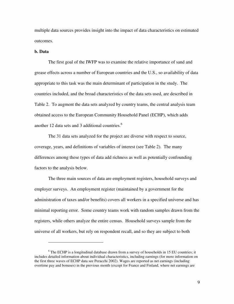
multiple data sources provides insight into the impact of data characteristics on estimated
outcomes.
b. Data
The first goal of the IWFP was to examine the relative importance of sand and
grease effects across a number of European countries and the U.S., so availability of data
appropriate to this task was the main determinant of participation in the study. The
countries included, and the broad characteristics of the data sets used, are described in
Table 2. To augment the data sets analyzed by country teams, the central analysis team
obtained access to the European Community Household Panel (ECHP), which adds
another 12 data sets and 3 additional countries.6
The 31 data sets analyzed for the project are diverse with respect to source,
coverage, years, and definitions of variables of interest (see Table 2). The many
differences among these types of data add richness as well as potentially confounding
factors to the analysis below.
The three main sources of data are employment registers, household surveys and
employer surveys. An employment register (maintained by a government for the
administration of taxes and/or benefits) covers all workers in a specified universe and has
minimal reporting error. Some country teams work with random samples drawn from the
registers, while others analyze the entire census. Household surveys sample from the
universe of all workers, but rely on respondent recall, and so they are subject to both
6 The ECHP is a longitudinal database drawn from a survey of households in 15 EU countries; it includes detailed information about individual characteristics, including earnings (for more information on the first three waves of ECHP data see Peracchi 2002). Wages are reported as net earnings (including overtime pay and bonuses) in the previous month (except for France and Finland, where net earnings are

10
sampling and reporting error. By contrast, employer salary surveys typically cover all
workers in the occupations and firms in their purview and draw their data from payroll
records, but vary considerably in how many occupations or firms they cover. The
employer surveys in the IWFP are particularly comprehensive because they are
conducted by national employer associations and are used extensively for policy and
managerial purposes.
Data sets also vary in terms of the compensation measure available. Some data
sets have base wages. However, most wage information in the IWFP is based on
monthly or annual labor earnings (that is, including base wage, overtime pay, and
bonuses). In those cases, we use a proxy for base wage: earnings divided by the best
available measure of hours worked. Hours worked information is available for most of
the data sources.
Samples are restricted to job stayers in order to concentrate on rigidity for
ongoing employment relationships. In addition, large outliers in wage changes7 are
excluded as they likely reflect wage reporting errors or unidentified job changes.
The time periods covered by the different data sets vary, with some starting in the
early 1970s and others running through the beginnings of the 2000s. In total, there are
360 data set-year observations, including observations from multiple data sets for Austria,
Belgium, Denmark, Finland, France, Germany, Italy, Norway, Portugal, Sweden,
Switzerland, and the U.K.
derived from reported gross data using a net/gross ratio). We exclude the series for Spain, Luxembourg and Sweden due to data limitations.

11
III. The dispersion of wage changes
This section examines the dispersion of wage changes in the IWFP data sets for
features consistent with the three interactions with inflation. Figure 1a shows a scatter
plot of the standard deviation of log (percentage) wage changes against the rate of wage
inflation for each year for each data set in our study. Both the magnitude of these
standard deviations and the range are remarkable. To some extent, the magnitude and
range are artifacts of a high average level of measurement error and of variation across
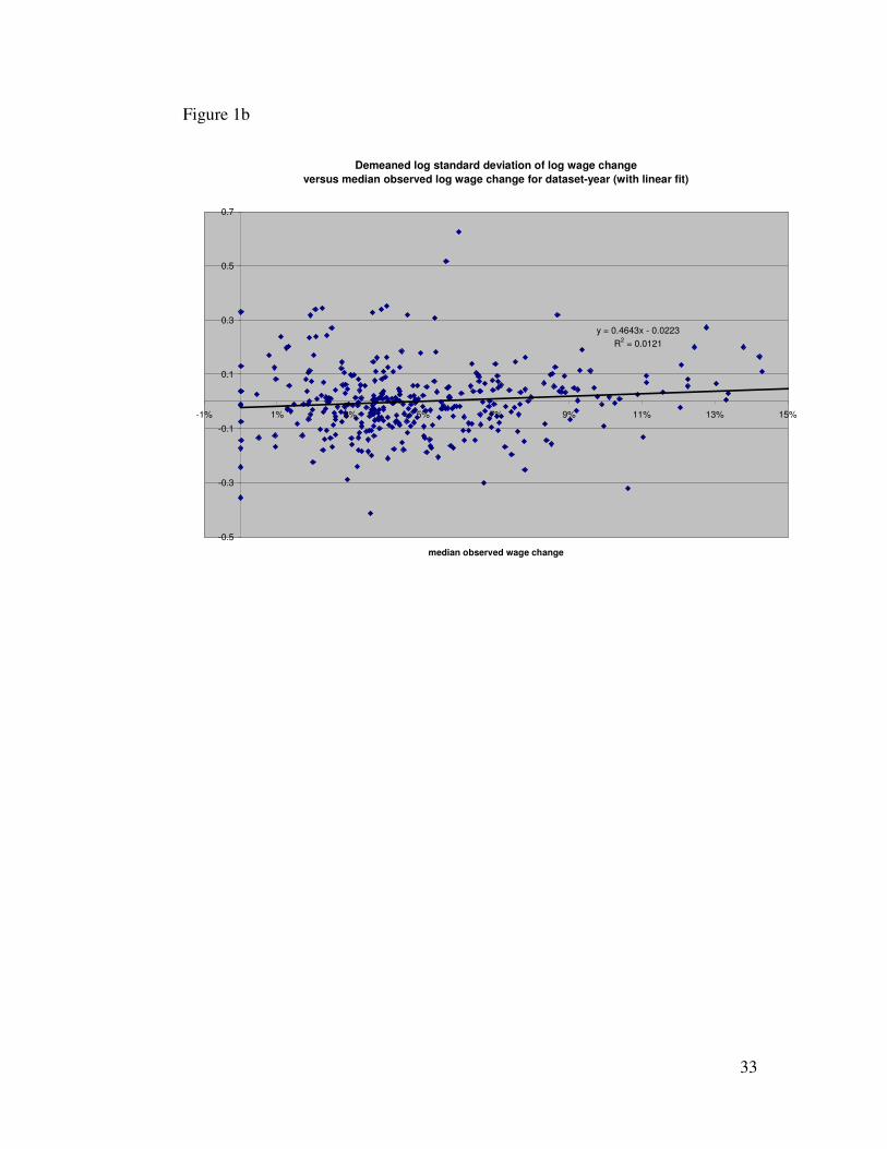
data sets in the extent of error. But as Figure 1b shows, even when the data set mean is
subtracted from the standard deviations (which should remove persistent differences due
to data set measurement error characteristics), there is still substantial variation.
Further, the linear relationships plotted in the two graphs suggest that inflation
plays a role in determining the extent of variation, as we would expect if either grease or
sand effects were present. The magnitude of inflation’s impact on wage change
dispersion is modest. A two standard deviation rise in inflation (+5.7 percentage points)
raises the dispersion of wage changes by about half of a standard deviation (or 2.1
percentage points). If grease or sand plays a role in the dispersion of wage changes, how
can we assess their roles in labor market performance?
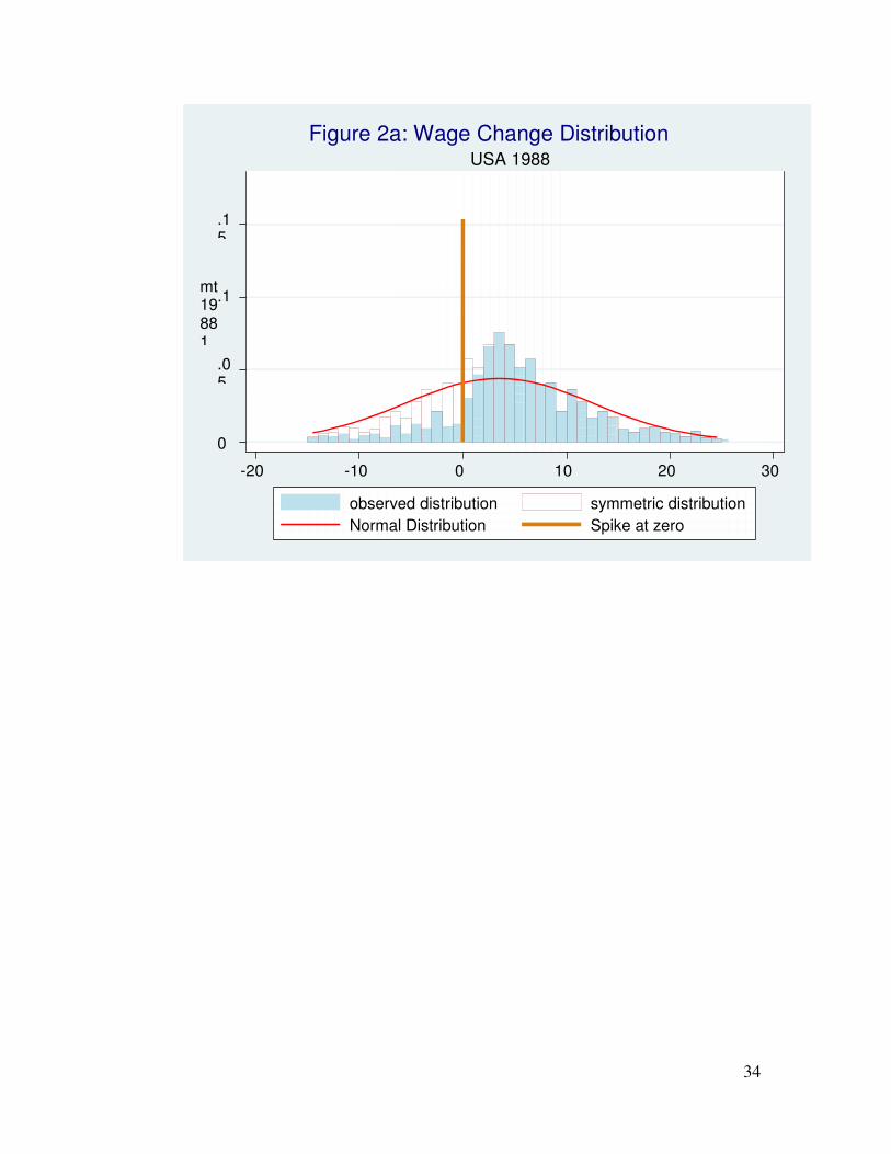
Histograms of wage changes offer a way to identify these effects more directly.
For example, Figure 2a presents the histogram of percentage wage changes for the U.S.
in 1988. It has four remarkable features:
• The histogram illustrates the substantial variation in wage changes among individuals that was shown to be common across all countries and years in Figure 1.
7 Increases of more than 60% in wage data or 100% in annual income data and cuts of more than 35% in wage data or 85% in income data were eliminated.
12
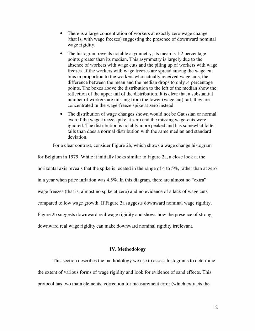
• There is a large concentration of workers at exactly zero wage change (that is, with wage freezes) suggesting the presence of downward nominal wage rigidity.
• The histogram reveals notable asymmetry; its mean is 1.2 percentage points greater than its median. This asymmetry is largely due to the absence of workers with wage cuts and the piling up of workers with wage freezes. If the workers with wage freezes are spread among the wage cut bins in proportion to the workers who actually received wage cuts, the difference between the mean and the median drops to only .4 percentage points. The boxes above the distribution to the left of the median show the reflection of the upper tail of the distribution. It is clear that a substantial number of workers are missing from the lower (wage cut) tail; they are concentrated in the wage-freeze spike at zero instead.
• The distribution of wage changes shown would not be Gaussian or normal even if the wage-freeze spike at zero and the missing wage-cuts were ignored. The distribution is notably more peaked and has somewhat fatter tails than does a normal distribution with the same median and standard deviation.
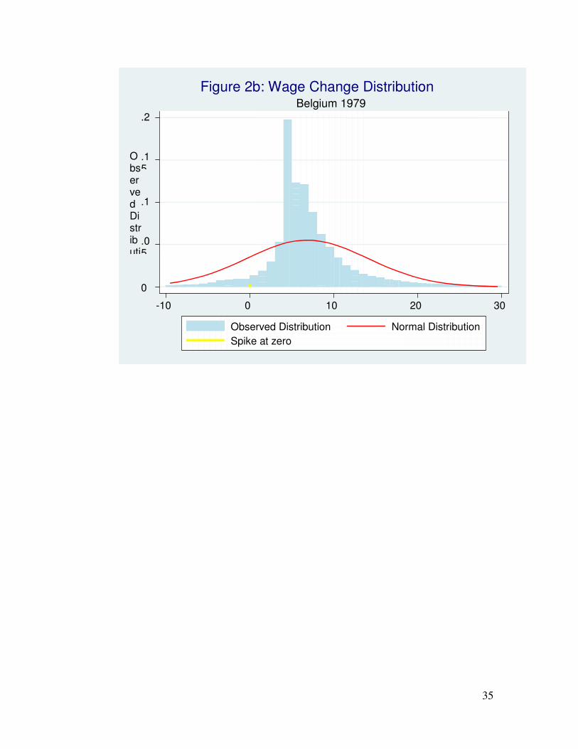
For a clear contrast, consider Figure 2b, which shows a wage change histogram
for Belgium in 1979. While it initially looks similar to Figure 2a, a close look at the
horizontal axis reveals that the spike is located in the range of 4 to 5%, rather than at zero
in a year when price inflation was 4.5%. In this diagram, there are almost no “extra”
wage freezes (that is, almost no spike at zero) and no evidence of a lack of wage cuts
compared to low wage growth. If Figure 2a suggests downward nominal wage rigidity,
Figure 2b suggests downward real wage rigidity and shows how the presence of strong
downward real wage rigidity can make downward nominal rigidity irrelevant.
IV. Methodology
This section describes the methodology we use to assess histograms to determine
the extent of various forms of wage rigidity and look for evidence of sand effects. This
protocol has two main elements: correction for measurement error (which extracts the
13
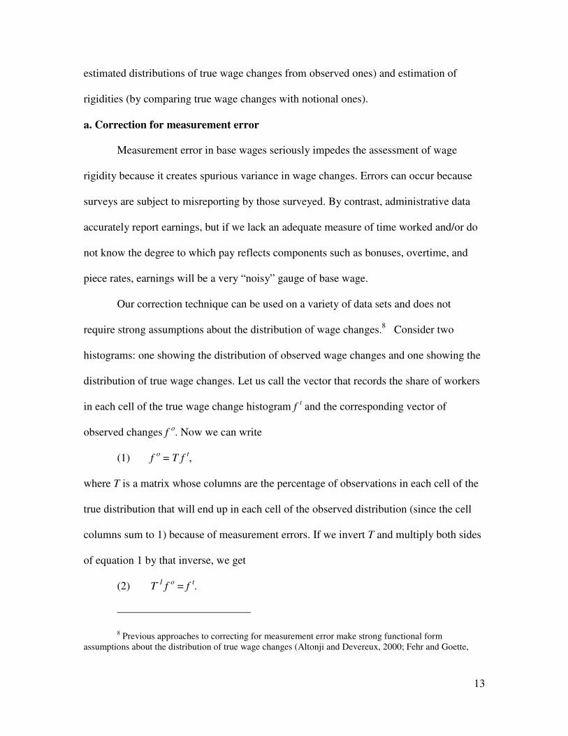
estimated distributions of true wage changes from observed ones) and estimation of
rigidities (by comparing true wage changes with notional ones).
a. Correction for measurement error
Measurement error in base wages seriously impedes the assessment of wage
rigidity because it creates spurious variance in wage changes. Errors can occur because
surveys are subject to misreporting by those surveyed. By contrast, administrative data
accurately report earnings, but if we lack an adequate measure of time worked and/or do
not know the degree to which pay reflects components such as bonuses, overtime, and
piece rates, earnings will be a very “noisy” gauge of base wage.
Our correction technique can be used on a variety of data sets and does not
require strong assumptions about the distribution of wage changes.8 Consider two
histograms: one showing the distribution of observed wage changes and one showing the
distribution of true wage changes. Let us call the vector that records the share of workers
in each cell of the true wage change histogram f t and the corresponding vector of
observed changes f o. Now we can write
(1) f o = T f t,
where T is a matrix whose columns are the percentage of observations in each cell of the
true distribution that will end up in each cell of the observed distribution (since the cell
columns sum to 1) because of measurement errors. If we invert T and multiply both sides
of equation 1 by that inverse, we get
(2) T-1 f o = f t.
8 Previous approaches to correcting for measurement error make strong functional form assumptions about the distribution of true wage changes (Altonji and Devereux, 2000; Fehr and Goette,

14
Thus, if we know T we can recover the true distribution from the observed
distribution. To construct T we assume that errors, when made, have a two-sided Weibull
distribution.9 We use method-of-moments to estimate the parameters of the error
distribution, the fraction of the population that is prone to errors, and the fraction of those
who are prone to errors that make errors in that period. We assume that the errors are
independent and that for the error-prone the probability of making an error is independent.
Most important, we assume that the true wage change is not auto-correlated so that we
can estimate the variance of the error from the negative auto-correlation of observed
wage changes.10
Dickens and Goette (2005) discuss the method and its assumptions in detail. Here,
we first note that Gottschalk’s (forthcoming) method for estimating true wage changes
also yields an error and a true wage series for each individual in his data set. We tested all
of our assumptions on those two series and could not reject any of them.
Further, application of this approach to IWFP data sets provides convincing
examples that the process works as intended. For example, the U.S. Panel Study of
Income Dynamics (PSID) and the ECHP are survey data sets where wages are reported
2005), or require high-frequency data on wage changes (Gottschalk, 2005) that are not available in most of the countries we study.
9 A two sided Weibull distribution is defined by the following cumulative density function:
��
��
�
−
≤=���
���
−
���
���
−
α
α
βµ
βµ
µx
x
eotherwise
exforxF5.1
5.)( .
The three parameters allow variation in the mean (µ), the dispersion (β), and the peakedness (α) of the distribution. The functional form provides a good fit to the empirical error distribution generated by Gottschalk’s (2005) method applied to U.S. Survey of Income Program Participation data.
10 In fact, there is evidence that wage changes over long periods of time are positively auto-correlated (Baker, Gibbs and Holmstrom 1994[0]). However this positive correlation is dwarfed by the
15
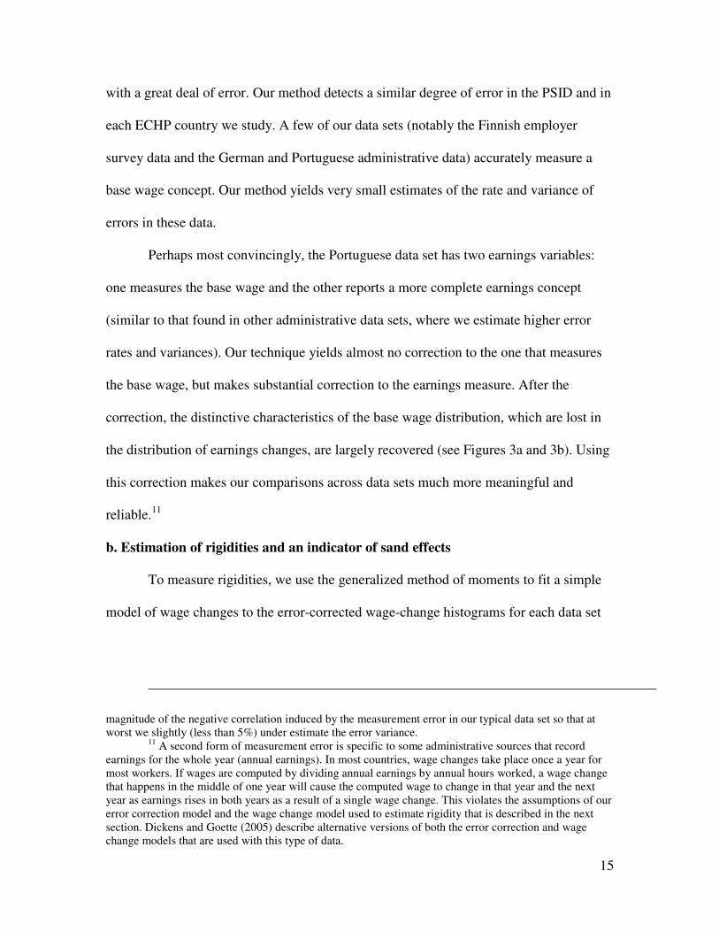
with a great deal of error. Our method detects a similar degree of error in the PSID and in
each ECHP country we study. A few of our data sets (notably the Finnish employer
survey data and the German and Portuguese administrative data) accurately measure a
base wage concept. Our method yields very small estimates of the rate and variance of
errors in these data.
Perhaps most convincingly, the Portuguese data set has two earnings variables:
one measures the base wage and the other reports a more complete earnings concept
(similar to that found in other administrative data sets, where we estimate higher error
rates and variances). Our technique yields almost no correction to the one that measures
the base wage, but makes substantial correction to the earnings measure. After the
correction, the distinctive characteristics of the base wage distribution, which are lost in
the distribution of earnings changes, are largely recovered (see Figures 3a and 3b). Using
this correction makes our comparisons across data sets much more meaningful and
reliable.11
b. Estimation of rigidities and an indicator of sand effects
To measure rigidities, we use the generalized method of moments to fit a simple
model of wage changes to the error-corrected wage-change histograms for each data set
magnitude of the negative correlation induced by the measurement error in our typical data set so that at worst we slightly (less than 5%) under estimate the error variance.
11 A second form of measurement error is specific to some administrative sources that record earnings for the whole year (annual earnings). In most countries, wage changes take place once a year for most workers. If wages are computed by dividing annual earnings by annual hours worked, a wage change that happens in the middle of one year will cause the computed wage to change in that year and the next year as earnings rises in both years as a result of a single wage change. This violates the assumptions of our error correction model and the wage change model used to estimate rigidity that is described in the next section. Dickens and Goette (2005) describe alternative versions of both the error correction and wage change models that are used with this type of data.
16
year.12 We assume that, in the absence of rigidity, log wage changes have a symmetric
two-sided Weibull distribution, referred to as the “notional” wage change distribution.
We estimate all three parameters of the notional distribution in each year.
We also assume that a fraction of the population is potentially subject to
downward real wage rigidity. If their notional wage change is below their (or their firm’s)
expected rate of inflation, they will receive a wage change equal to that expected rate of
inflation rather than equal to their notional wage change. The mean and standard
deviation of the expected rate of inflation for each country in each year are also
parameters of the model and are estimated separately for each year.
We next assume that a fraction of the population is potentially subject to
downward nominal wage rigidity. Such workers who have a notional wage change of less
than zero, and who are not subject to downward real wage rigidity, receive a wage freeze
instead of a wage cut.
Finally, since there is often a paucity of observations just above zero as well as
just below it (see Figure 2a), we allow that some people are subject to symmetric nominal
wage rigidity. This can be the result of the costs of revising pay schedules or a tendency
to round off wage changes. If such people have a notional wage change close to zero and
are not affected by downward real wage rigidity, they will receive a wage freeze rather
than a small positive or negative change. We control for this possibility to avoid
overestimating the role of downward nominal wage rigidity. However, because we doubt
12 The IWFP has experimented with a number of other methods for identifying differing degrees of rigidity (Dickens and Goette 2004) requiring less restrictive assumptions. The other methods were judged inferior in that deviations from this more restrictive method seemed to result from shortcomings of the alternative methods rather than from failures of the distributional assumptions critical to the method used here.
17
that this symmetric nominal rigidity is economically important, we do not address it in
the analysis that follows.
This process yields estimates of the extent of downward nominal wage rigidity (n)
and of downward real wage rigidity (r). These measures vary between 0 and 1, where 0
indicates perfect flexibility (no one is constrained) and 1 indicates full rigidity (all
workers are potentially constrained). The protocol also yields estimates of the dispersion
of notional wage changes that we can examine for evidence of sand effects.
V. Rigidity estimates
When we apply the method, described in the previous section, to estimating
rigidity for each data set for each year, we find a great deal of variation across time and
data sets. Before proceeding with further analysis, we examine the validity of this
variation.
Focusing first on cross-country evidence, we find considerable variation across
countries in the extent of both real and nominal rigidity when we average across all data
sets and time for each country (see Figure 4).Estimates of the fraction of workers
potentially affected by downward nominal wage rigidity range from 9% to 66%, while
the comparable range for real rigidity is 3% to 52%. Countries with higher nominal
rigidity tend to show less real rigidity, although the correlation of country averages is
only a statistically insignificant -0.24. Regressions (not reported here) of our annual
estimates of downward nominal wage rigidity and downward real wage rigidity on
country effects show them to be jointly significant even after controlling for a full set of
18
data set characteristics.13 In addition, the data set characteristics explain a minor part (less
than 5 percent) of the variation in these regressions. This suggests that the error
correction procedure does a good job of removing the influence of data set characteristics
on our rigidity measures.
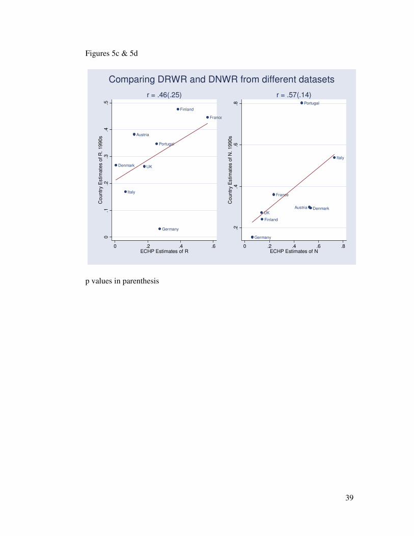
Figures 5a, b, c and d compare these measures to those from other studies and
between different data sets in our study. We find that n (our measure of the fraction of
workers who might be affected by nominal rigidity) is strongly positively correlated with
similar measures from two other cross-national studies that use different methodologies
to estimate the extent of downward nominal wage rigidity (Figures 5a and b).14
Furthermore, in countries where we have r and n estimates from the ECHP and another
data set the two are strongly positively correlated (0.54 for r and 0.60 for n) (Figures 5c
and d). Since the paired estimates in all four figures cover different time periods, and in
some cases different types of workers, we do not expect a perfect correlation. Overall, we
consider these results to be very supportive of the reliability of our country average
estimates.
Validation of the variation of our country estimates over time is difficult;
nevertheless, they do receive support in a number of cases. Our ability to validate
systematically is limited because we have no comparable alternative cross-country
studies and because there is little or no overlap between the time periods covered by the
different data sets for the same countries in our study.
13 The data set characteristic include indicator variables for the following: census vs. sample, survey vs. administrative records, earnings vs. wage data, whether the country team ran the annual earnings protocol vs. the wage protocol, whether the data was drawn from the ECHP, and whether hours worked were available.
19
However, some of the notable changes that we observe in smoothed measures of
rigidity happen at the same time that important institutional changes in the country occur.
For example, our estimate of the fraction of workers affected by real wage rigidity in the
U.S. declines from nearly 20% in the 1970s to zero in the mid-1980s and 1990s. This
decline corresponds to the decline in the role of unions and pattern bargaining in U.S.
wage setting (Blanchflower and Freeman, 1992). Declines in the importance of real
rigidity in Germany and Italy also coincide with significant changes in the wage setting
institutions in those countries (declining union power in Germany and the elimination of
indexation in Italy--see Bauer et al. 2003 and Devicienti et al. 2005, respectively).
On the other hand, for several countries our rigidity measures show volatility over
short periods of time that seems implausible. Examination of these cases suggests two
causes that may be correctible in future research. First, our measure of symmetric
nominal rigidity depends on the number of observations in the cells just around zero.
This effect becomes difficult to disentangle from downward real rigidity when inflation
rates are very low with consequences for the measurement of downward nominal rigidity
as well.
Second, our concept of downward real wage rigidity may be difficult to
distinguish empirically from another common feature of wage determination. Some
important centralized wage bargains set a floor for wage changes while allowing
decentralized changes above the floor (sometimes called “wage drift”). In those cases,
the histogram for wage changes resembles that for downward real wage rigidity, although
14 We drop Holden and Wolfsburg’s implausible estimate for the U.S. where they estimate the fraction subject to nominal rigidity to be negative. If we include it and set it to the lower bound of zero the correlation with our measure drops from .66 to .43.
20
the spike will reflect not only the expected rate of inflation, but also the negotiated
minimum real wage change. Our protocol restricts the expected rate of inflation to fall
within what we consider reasonable bounds for such an expectation. For countries with
this sort of wage drift, we can estimate considerable real wage rigidity in years when the
floor falls within a preset range for expected inflation, but not in years when the floor is
above that range. This inconsistency will also have spillover effects on our estimates of
nominal rigidity.
VI. Correlates of rigidity
We now explore whether our measures of wage rigidity are associated with labor
market institutions that are suspected sources of wage rigidity. We consider the
following six labor market institutions: strictness of employment protection legislation
(EPL), union density, collective bargaining coverage, whether minimum wage or wage
indexation legislation is in place, and the degree of corporatism (an index of bargaining
coordination and centralization). Our most robust results are for measures of unionism.
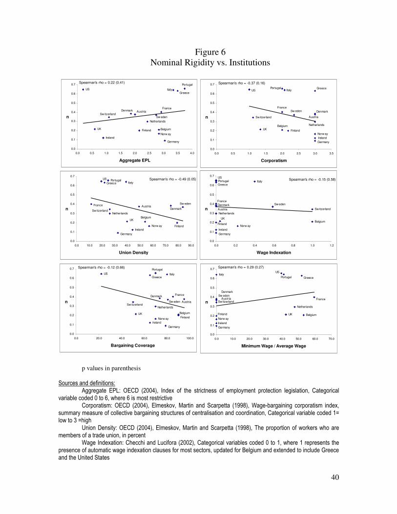
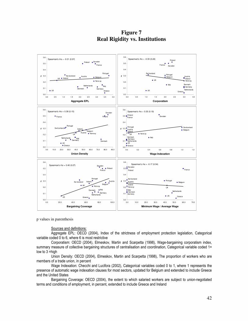
Figures 6 and 7 show scatter plots of country averages of n and r against six
measures of labor market institutions. We see that the index of EPL has a weak,
statistically insignificant positive correlation with both our measures of wage rigidity.
The corporatism index—which is a summary measure of centralization and coordination
bargaining structures—has a statistically insignificant negatively correlated with both
nominal and real rigidity, suggesting only weak support for the hypothesis that more
centralized and coordinated unions exert less wage pressure. Our measure of indexation
is weakly negatively correlated with nominal rigidity and positively correlated with real
rigidity though neither relationship is statistically significant. The signs and relative

21
magnitudes are what we would expect and the weakness of the result not surprising since
all indexation regimes in our sample provide only partial coverage of the economy. Also,
some countries such as Finland and France experience relatively high real rigidity
without ever having had wage indexation clauses in place.
The figures also show that countries with higher ratios of minimum wages to
average wages have modestly higher levels of nominal rigidity and lower levels of real
rigidity. However, this result seems to be driven by the contrast between countries with
substantial collective bargaining but no minimum wages, and those with substantial
minimum wages. This suggests that the relationship is only a reflection of the much
stronger and more robust correlation between union power and rigidity.
The strongest results are for union coverage and union density, though even with
these variables the correlations are only statistically significant at the 10% level in a one-
tailed test. We speculate that union representation raises worker awareness of what is
happening to their real wages and gives them the bargaining power to protect their real
wages. Accordingly, workers become less concerned with nominal wage changes.
Alternatively, unions may achieve only partial real rigidity for some workers; that is, they
may cause some wage freezes to become nominal wage increases, albeit real wage cuts.
Under these circumstances we would estimate a lower rate of nominal rigidity.
VII. Does wage rigidity cause unemployment?
We now consider the consequences of wage rigidity. If nominal rigidity causes
some unemployment at very low rates of inflation, small increases in inflation can reduce
this joblessness, creating the grease effect. However, in cases where it is real rigidity that
22
reduces employment, and many workers are potentially affected, the grease effect of
inflation can be mitigated. To examine the relationship between wage rigidity and
unemployment we turn to the general equilibrium model of Akerlof, Dickens and Perry
(1996) that motivates a Phillips curve relation of the form
(3) �t = �te + c - a Ut + b St + xt.
In their model, �t is the rate of price inflation at time t, �te is the expected rate of
price inflation, c is a constant, Ut is the unemployment rate, St represents the wage effects
of rigidity, and xt is the effects of supply shocks. This relationship implies that
(4) Ut = St b/a + [c +xt - (�t - �te)]/a.
The constant b is equal to 1 plus the average mark-up of prices over labor costs. Typical
estimates of the coefficient a place it between 0.2 and 1.0, so we would expect the impact
of St on unemployment to be greater than 1.0.
The wage rigidity variable (St) is the amount by which nominal wages of those
constrained by downward rigidity are higher as a result of wage rigidity, multiplied by
their share of the wage bill. For each data set for each year, we approximate St by
estimating the extent to which wage rigidity raised average wage changes, as compared to
the notional wage change distribution for that data-set-year.15
15 To be explicit, we compute a numerical estimate of the average notional log wage change conditional on the wage change being negative. We also compute the average log wage change conditional on it being less than our estimate of the average expected rate of inflation. The latter average wage change is multiplied by a smoothed estimate of the fraction of the workforce potentially subject to downward real wage rigidity (r). Similarly, the former average wage change is multiplied by a smoothed estimate of the fraction of the workforce potentially affected by downward nominal rigidity times one minus the fraction potentially subject to real rigidity ([1-r]n). These are summed to obtain to obtain an approximation of St. This is only an approximation because, as Akerlof, Dickens and Perry show, the effects of rigidity can
23
We estimate both equation (3) and equation (4). In estimating equation 3 we
assume that the expected rate of inflation is equal to the previous period’s inflation and
that the effect of supply shocks can be captured by indicator variables for specific events
(oil shocks) or for all years. In estimating equation 4, we implicitly assume that
expectation errors are orthogonal to St by excluding inflation or expectations from the
regression.
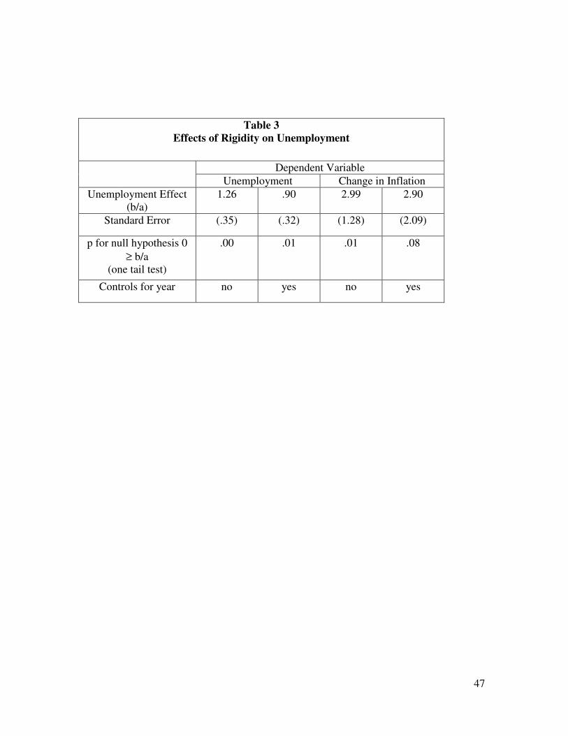
We run two specifications for each equation. All specifications include data-set-
specific intercepts and the second specification also includes year-specific intercepts to
control for common supply shocks. Table 3 presents the results.
In all but one case, the estimate of the unemployment impact (b/a) is greater than
1 and in all cases is statistically significantly greater than zero at least at the 0.1 level.
When we separately estimate the effects of real and nominal rigidity (regressions not
reported), some of the estimates are not statistically significantly greater than zero, but
we can never reject the hypothesis that the unemployment effect of a rigidity measure is
greater than 1, nor can we reject the hypothesis that the coefficients on the two measures
of the wage impact of rigidity are equal. Also, when we estimate b independent of a in
equation 3 (regressions not reported), it is always less than the predicted minimum of 1,
but we can never reject the hypothesis that it is greater than 1. Taken together, these
results provide moderately strong evidence that inflation can lower unemployment in the
presence of downward nominal wage rigidity (that is, of grease effects) as well as the
inability of inflation to lower unemployment in the presence of downward real wage
accumulate over time if a large fraction of the workforce is affected by the rigidity. This normally is not important, but it can be during extended periods of low inflation or deflation such as the Great Depression in the U.S.

24
rigidity. The size of the grease effects is in the range predicted by the Akerlof, Dickens
and Perry model.
VIII. Sand estimates
We turn now to the sand effects of inflation and productivity growth. It is difficult
to create a direct estimate of the sand that would focus on unintended variation in wage
changes that could be applied to all of the IWFP datasets. Thus, we examine our
measures of notional wage change variability (from which the impact of wage rigidities
and reporting errors have been removed) for any remaining correlation with expected or
unexpected inflation. We find weak evidence that high and variable inflation, in
particular, distorts price signals in labor markets.
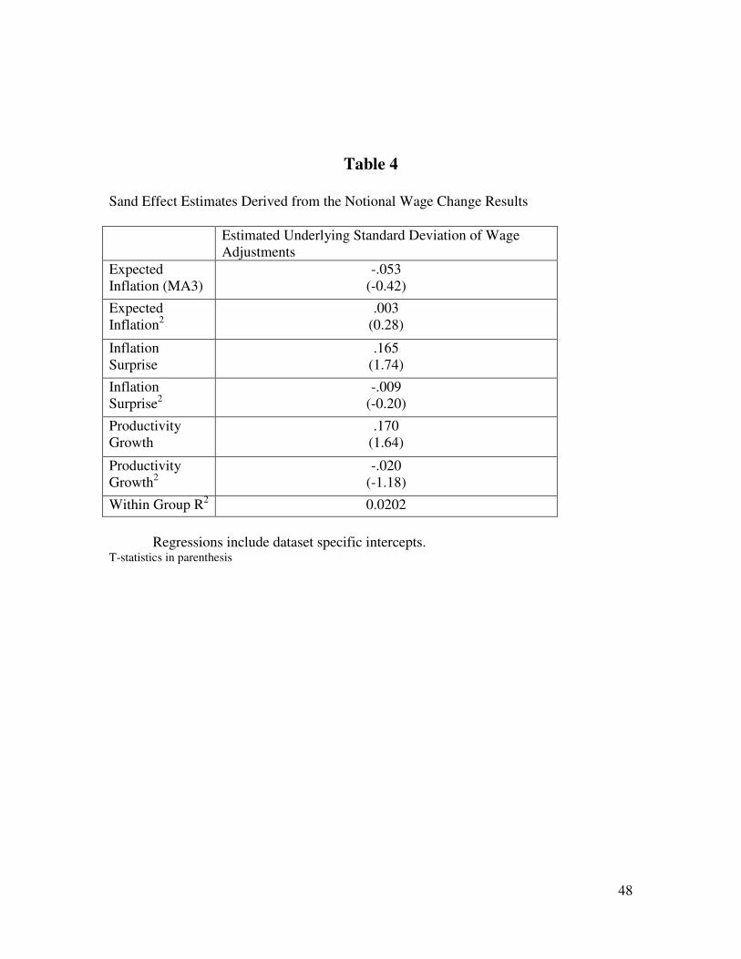
The first column of Table 4 reports the relationship between the standard
deviation of changes in the log of notional wages and inflation expectations, inflation
surprises, and productivity growth.16 Only the inflation surprise proxy is statistically
significant at the 5 percent level (one-tail test), and there is little evidence that these
effects taper off as the second order term is not statistically significant. The effects of
expected inflation on the standard deviation of the notional wage are minimal; while
productivity growth, which is difficult to predict, yields similar coefficients to inflation’s
surprises. This is consistent with the proposition that higher unexpected inflation distorts
price signals.
16 We measure expected inflation as a three year moving average of realized inflation rates. Several other expectations measures produced similar coefficient estimates, but the standard errors were larger

25
To gauge the size of misallocation effects of inflation on the labor market, we
estimate regressions similar to those reported in Table 3, including the standard deviation
of notional wage change on the right hand side both with and without the measures of
rigidity effects. Coefficients were small and statistically insignificant in nearly all
specifications, and in the few cases where they were significant they have the wrong
sign.17 Of course, the costs and misallocation effects of inflation need not show up as
unemployment, and it is difficult to assess the magnitude of the effects without a detailed
structural model of firm wage setting.
IX. Conclusion
The International Wage Flexibility Project has investigated three ways in which
labor market imperfections can interact with inflation. First, moderate inflation in the
presence of resistance to nominal wage cuts can “grease” the wheels of relative wage
adjustment to ongoing shocks and thus improve economic efficiency. Second, widespread
resistance to real wage cuts can also raise unemployment rates, but in this case inflation
provides no relief. Third, inflation can cause distortions in relative wages that lead to
costly resource misallocations, thus throwing “sand” in the wheels of economic
adjustment. While the first effect has been studied extensively, especially in the U.S., the
other two have not.
The IWFP investigates these three effects simultaneously using 31 panel data sets
covering individual workers in 16 European countries and the U.S., relying on the
expertise, data access, and analysis contributed by 13 country teams. We find
17 The coefficients on the rigidity effects variables are virtually unaffected by the inclusion of this
26
considerable variation in wage changes among workers in the same country and year. The
variation increases with inflation, as we would expect if either downward nominal
rigidity or sand effects were important.
Applying a new estimator for the prevalence of these three effects, we also find
evidence of both types of rigidity in nearly every country. Estimates of the fraction of
workers potentially affected by downward nominal wage rigidity range from 9% to 66%,
while the comparable range for real rigidity is 3% to 52%. Furthermore, there is some
evidence that countries with higher nominal rigidity tend to show less real rigidity.
Our technique and wealth of data sets enable us to explore the impact of data
features on empirical estimates of wage rigidity and compare our results with those of
previous studies. Our method for correcting wage change histograms should make results
comparable across different data sets. Indeed, the contribution of data set characteristics
to explaining the variation in our rigidity measures across countries and across time is
minimal, and results derived from the European Community Household Panel and those
from country-specific data sets are strongly correlated. In addition, our measures of
downward nominal rigidity are strongly correlated with other recent measures derived
from industry or individual data.
Our examination of the causes of downward nominal and real wage rigidity
suggests an important role for the extent of unionization and collective bargaining
coverage. Both show a consistently positive relationship with the extent of downward
real wage rigidity and a negative association with downward nominal wage rigidity. This
finding suggests that collective bargaining focuses workers’ attention on real wages and
variable and no substantive conclusions are altered.
27
gives them some ability to resist real wage cuts. Other institutional variables that we
examined had weaker relationships with our measures of rigidity.
These differences in rigidity across countries may translate into differences in
unemployment. Measures of the “wage impact” of downward nominal and real wage
rigidity (that is, the extent to which workers’ wages are affected in a particular year) are
positively related to unemployment with statistically significant coefficients of about the
size predicted by theory.
Finally, we find only suggestive evidence of potential sand effects in notional wage
change distributions. The dispersion of these notional adjustments is positively correlated
with unexpected inflation, consistent with the view that the increased dispersion reflects
more, or more serious, errors in firm wage setting. In addition, we find no evidence of
unemployment effects from degradation of price signals, so any costs imposed may be on
productivity rather than on jobs.
28
References
Akerlof, George A., William T. Dickens, and George L. Perry (1996). “The Macroeconomics of Low Inflation.” Brookings Papers on Economic Activity 1, 1-75.
Alogoskoufis, George S. and Alan Manning (1988). “On the Persistence of
Unemployment,” Economic Policy, 7, 428-469. Altonji, Joseph G., and Paul J. Devereux (2000). “The Extent and Consequences of
Downward Nominal Wage Rigidity.” In S. Polachek (ed.). Worker Well-Being, # 7236, Elsevier.
Baker, George., Michael Gibbs and Bengt Holmstrom (1994). “The Wage Policy of a
Firm,” Quarterly Journal of Economics 109, 921-955. Barwell, Richard and Mark E. Schweitzer (2005). “The Incidence of Nominal and Real
Wage Rigidity in Great Britain: 1978–1998.” Federal Reserve Bank of Cleveland Working Paper 05-08.
Bauer, Thomas, Holger Bonin, and Uwe Sunde (2003): “Real and Nominal Wage
Rigidities and the Rate of Inflation: Evidence from West German Micro Data”, IZA working paper 959.
Bewley, Truman F., (1999). Why Do Wages Not Fall During a Recession? Harvard
University Press. Blanchflower, David and Freeman, Richard (1992). “Unionism in the U.S. and in Other
Advanced OECD Countries”, Industrial Relations 31, pages 56-79 Blinder, Alan S. and Don H. Choi (1990). “A Shred of Evidence on Theories of Wage
Stickiness,” Quarterly Journal of Economics, vol. 105, no. 4 (November ), pp. 1003-1015.
Bound, John and Alan B. Krueger (1991). “The Extent of Measurement Error in
Longitudinal Earnings Data: Do Two Wrongs Make a Right?” Journal of Labor Economics (9)1: 1-24.
Bullard, James, and John W. Keating (1995). “The Long-run Relationship between
Inflation and Output in Postwar Economies.” Journal of Monetary Economics 36, 477-496.
Böckerman, Petri, Seppo Laaksonen and Jari Vainiomäki (2003). “Who Bears the Burden
of Wage Cuts? Evidence from Finland During the 1990s.” working paper, University of Tampere.

29
Camba-Mendez, Gonzalo, Juan García, and Diego Rodríguez Palenzuela (2003). “Relevant Economic Issues Concerning the Optimal Rate of Inflation.” Background Studies for the ECB’s Evaluation of its Monetary Policy Strategy, European Central Bank.
Dessy, Orietta (2005). “Nominal Wage Rigidity in Europe: Estimates, Causes and
Consequences.” Mimeo, University of Milan. Devicienti, Francesco, Agata Maida, and Paolo Sestito (2005). “Nominal and Real
Rigidity: Micro Based Measures and Implications,” Mimeo, University of Torino. Dickens, William T. (2001). “Comment on Charles Wyplosz, Do We Know How Low
Inflation Should Be?” in Alicia G. Herrero, Vitor Gaspar, Lex Hoogduin, Julian Morgan, and Bernhard Winkler eds. Why Price Stability? Proceedings of the Frist ECB Central Banking Conference, November 2000, Frankfurt Germany ECB: Frankfurt.
Dickens, William T. and Lorenz Goette (2004). “Notes on Estimating Wage Rigidity,”
Brookings mimeo. Dickens, William T. and Lorenz Goette (2005). “Estimating Wage Rigidity for the
International Wage Flexibility Project,” Brookings mimeo. Djoudad, R., and Thomas C. Sargent (1997). “Does the ADP Story Provide a Better
Phillips Curve for Canada?” Working Paper, Economic Studies and Policy Analysis Division, Department of Finance, Ottawa, October.
EIRO (2005) – The European industrial relations observatory online -
http://www.eiro.eurofound.eu Elmeskov, Jorgen, John P. Martin and Stefano Scarpetta (1998). "Key Lessons for
Labour Market Reforms: Evidence from OCED Countries' Experiences", Swedish Economic Policy Review, 5, 205-252
Elsby, Michael (2004). “Evaluating the Economic Significance of Downward Nominal
Wage Rigidity.” Mimeo, London School of Economics. Fehr, Ernst and Lorenz Goette (2005). Robustness and Real Consequences of Nominal
Wage Rigidity. Journal of Monetary Economics 52, 779-804. Fortin, Pierre (1996). “The Great Canadian Slump,” Canadian Journal of Economics 29,
November, 761-87. Friedman, Milton (1977). “Nobel Lecture: Inflation and Unemployment,” Journal of
Political Economy, vol. 85, no. 3, pp. 451-472.

30
Gottschalk, Peter (forthcoming). "Downward Nominal Wage Flexibility: Real or Measurement Error?" Review of Economics and Statistics.
Groshen, Erica and Mark Schweitzer (1999). “Identifying Inflation’s Grease and Sand
Effects in the Labour Market in Martin Feldstein, ed. The Costs and Benefits of Price Stability, (Chicago: Univ. of Chicago Press).
Groshen, Erica L. and Mark E. Schweitzer (2000). “The Effects of Inflation on Wage
Adjustments in Firm-Level Data: Grease or Sand?” Federal Reserve Bank of New York Staff Report No. 9, January 1996 (Revised version: June 2000).
Holden, Steinar (2004). "Wage Formation Under Low Inflation". In Collective
Bargaining and Wage Formation - Challenges for an European Labour Market, H. Piekkola and K. Snellman (eds.), Springer-Verlag, pp 39-58.
Holden, Steinar and Fredrik Wulfsberg (2005). Downward Nominal Wage Rigidity in the
OECD. Mimeo, available at http://folk.uio.no/sholden/#wp Kaufman, Roger T. (1984). “On Wage Stickiness in Britain’s Competitive Sector.”
British Journal of Industrial Relations 22, 101-112. Keynes, John Maynard (1936). The General Theory of Employment, Interest and Money. Knoppik, Christoph and Thomas Beissinger (2005). “Downward Nominal Wage Rigidity
in Europe: An analysis of European Micro Data from the ECHP 1994-2001.” IZA DP # 1492.
Layard, Richard, Stephen Nickell, and Richard Jackman (1991). Unemployment:
Macroeconomic Performance and the Labour Market. Oxford University Press. Lebow, David E., Raven E. Saks, Beth A. Wilson (2003). “Downward Nominal Wage
Rigidity. Evidence from the Employment Cost Iindex.” Advances in Macroeconomics vol. 3, Issue 1, article 2.
Nickell, Stephen J. and Glenda Quintini (2003). “Nominal Wage Rigidity and the Rate of
Inflation.” The Economic Journal 113, 762-781. OCED (2004). "Wage Setting Institutions and Outcomes" Chapter 3 in the OECD
Employment Outlook. Peracchi, F. (2002). “The European Community Household Panel: A Review”, Empirical
Economics 27, pp. 63-70. Reinsdorf, Marshall (1994). “New Evidence on the Relation between Inflation and Price
Dispersion,” American Economic Review, vol. 84, no. 3, pp. 720-731.

31
Sheshinski, Eytan and Yoram Weiss (1977). “Inflation and Costs of Price Adjustment,” Review of Economic Studies, vol. 44, no. 2 pp. 287-303.
Slichter, Sumner and Heinz Luedicke (1957). “Creeping Inflation—Cause or Cure?”
Journal of Commerce, pp. 1-32. Smith, J.C. (2000). “Nominal Wage Rigidity in the United Kingdom,” Economic Journal
110(462): C176-C195. Stigler, George J. and James K. Kindahl (1970). The Behavior of Industrial Prices,
National Bureau of Economic Research General Series No. 90 (New York: Columbia University Press).
Tobin, James (1972). “Inflation and Unemployment,” American Economic Review, vol.
62, no. 1, pp. 1-18. Vining, Daniel R. and Thomas C. Elwertowski (1976). “The Relationship between
Relative Prices and the General Price Level,” American Economic Review, vol. 66, no. 4, pp. 699-708.
Wilson, Beth Anne, (1999). “Wage Rigidity: A Look Inside the Firm,” April 16, FEDS
Working Paper No. 99-22 http://ssrn.com/abstract=165588

32
Figure 1a
Demeaned log standard deviation of log wage change versus median observed log wage change for dataset-year (with linear fit)
y = 0.4643x - 0.0223R2 = 0.0121
-0.5
-0.3
-0.1
0.1
0.3
0.5
0.7
-1% 1% 3% 5% 7% 9% 11% 13% 15%
median observed wage change
33
Figure 1b
Demeaned log standard deviation of log wage change versus median observed log wage change for dataset-year (with linear fit)
y = 0.4643x - 0.0223R2 = 0.0121
-0.5
-0.3
-0.1
0.1
0.3
0.5
0.7
-1% 1% 3% 5% 7% 9% 11% 13% 15%
median observed wage change
34
0
.05
.1
.15
mt19881
-20 -10 0 10 20 30
observed distribution symmetric distributionNormal Distribution Spike at zero
USA 1988Figure 2a: Wage Change Distribution
35
0
.05
.1
.15
.2
ObservedDistributi
-10 0 10 20 30
Observed Distribution Normal DistributionSpike at zero
Belgium 1979Figure 2b: Wage Change Distribution

36
Bas e W a ges
- 0.0 2
0
0.0 2
0.0 4
0.0 6
0.0 8
0. 1
0.1 2
-25 -2 3 -2 1 -1 9 - 17 - 15 -1 3 -11 - 9 -7 -5 -3 -1 1 3 5 7 9 1 1 13 15 1 7 1 9 2 1 23 25 27 29 3 1 33 35 37 39 4 1 4 3 45 47 49
Figure 3aPortuguese Wa ge Cha nge H is togra ms 1994
T o ta l E a r ni n gs
-0 . 02
0
0 . 02
0 . 04
0 . 06
0 . 08
0 .1
0 . 12
-2 5 -2 3 - 21 -1 9 -1 7 - 15 -1 3 - 11 -9 - 7 -5 -3 - 1 1 3 5 7 9 11 1 3 1 5 17 1 9 2 1 23 2 5 2 7 29 3 1 33 3 5 3 7 39 4 1 4 3 45 4 7 4 9
T o t a l E a r n i n g s
-0 . 0 1
0 . 0 1
0 . 0 3
0 . 0 5
0 . 0 7
0 . 0 9
0 . 1 1
0 . 1 3
0 . 1 5
- 2 5 - 2 3 -2 1 -1 9 -1 7 -1 5 -1 3 -1 1 - 9 - 7 -5 -3 -1 1 3 5 7 9 1 1 1 3 1 5 1 7 1 9 2 1 2 3 2 5 2 7 2 9 3 1 3 3 3 5 3 7 3 9 4 1 4 3 4 5 4 7 4 9
B a s e W a g e s
- 0 .0 1
0 .0 1
0 .0 3
0 .0 5
0 .0 7
0 .0 9
0 .1 1
0 .1 3
0 .1 5
-2 5 - 2 2 - 1 9 -1 6 - 1 3 - 1 0 - 7 - 4 - 1 2 5 8 1 1 1 4 1 7 2 0 2 3 2 6 2 9 3 2 3 5 3 8 4 1 4 4 4 7 5 0
Figure 3bPortuguese Wa ge Cha nge H is togra ms 1992
Blue bars are Observed Frequenc ies and red bars are the Correc ted Frequenc ies.

37
Figure 4
0.2
.4.6
.8
Greec
e US
Nether
lands
German
y
Denmar
kIta
ly
Norway UK
Irelan
d
Austria
Belgium
Portug
al
Switzer
land
Franc
e
Finlan
d
Sweden
Real and Nomial Ridigity by Country
Read Rigidity Nominal Rigidity

38
Figure 5a & b
AustriaBelgium
Denmark
Finland
FranceGermany
Greece
Ireland
Italy
Portugal
UK
0.2
.4.6
.81
KB
DN
WR
0 .2 .4 .6 .8IWFP N
Knoppik and Beissinger r=.56(.07)
Austria
Belgium
DenmarkFinland
France
Germany
Greece
Ireland
Italy
Netherlands
Norway
Portugal
Sweden
UK0
.2.4
.6.8
1H
W D
NW
R
0 .2 .4 .6 .8IWFP N
Holden and Wulfsberg r= .66(.01)
Source: HW (2005) FWCP from Table B1, page 38; KB (2005) Table 4, page 29 and IWFP.
p values in parenthesis
39
Figures 5c & 5d
Austria
Denmark
Finland
France
Germany
Italy
Portugal
UK
0.1
.2.3
.4.5
Cou
ntry
Est
imat
es o
f R. 1
990s
0 .2 .4 .6ECHP Estimates of R
r = .46(.25)
Austria Denmark
Finland
France
Germany
Italy
Portugal
UK
.2.4
.6.8
Cou
ntry
Est
imat
es o
f N. 1
990s
0 .2 .4 .6 .8ECHP Estimates of N
r = .57(.14)
Comparing DRWR and DNWR from different datasets
p values in parenthesis
40
Figure 6 Nominal Rigidity vs. Institutions
p values in parenthesis
������������� � ����� � � ��� ��� � � � �� � � � � � �� � � � ��� ���� � ��� � �� ��� ������ ��� �! " #�$ ! ��� " ������ �� #�� �#� ��� � ��� �� �#�
% � & #��������� ����' ��( ����' � ��! ��������� �� % ���� ��" ��� �! �� � � � � � �� � � � ��� � #! ��) �% �� * �� � �� ���" ���� �+ , , - ��� . � �/& �� � � ���" ��� �! � ��� ��
��! ! �$ �! �����������##��� % ��& �� � �������������������# �� ��������� � ���� ��� �� �#�% � & #��������+ 0 �#�( ����1 �0 � ��
2 �� � �� �$ �� � � � � � �� � � � ��� � #! ��) �% �� * �� ������" ���� �+ , , - ��� 3 �� " ��" ��� ����� ( ��) ���� ( �����! �! & �������������� ��� �" ������
. � ������ � ���� ��� ���� �� ������ � � � ��� � ��� �� �#�% � & #���������� � ���+ �� ( ����+ ���" �������� ��" �������������! � ��( � �� ��� � ���#���������! ��������������" ���������4 �#� �! ����� ��������� �#����5 ��������� ��2 ����������
UK
Sw eden
Portugal
Norw ay
Italy
IrelandGermany
USGreece
France
Finland
Sw itzerlandDenmark
Belgium
Austria
Netherlands
Spearman's rho = 0.22 (0.41)
0.0
0.1
0.2
0.3
0.4
0.5
0.6
0.7
0.0 0.5 1.0 1.5 2.0 2.5 3.0 3.5 4.0
Aggregate EPL
n
UK
Sw eden
Portugal
Norw ay
Italy
IrelandGermany
USGreece
France
Finland
Sw itzerland
Denmark
Belgium
Austria
Netherlands
Spearman's rho = -0.37 (0.16)
0.0
0.1
0.2
0.3
0.4
0.5
0.6
0.7
0.0 0.5 1.0 1.5 2.0 2.5 3.0 3.5
Corporatism
n
UK
Sw eden
Portugal
Norw ay
Italy
IrelandGermany
USGreece
France
Finland
Sw itzerlandDenmark
Belgium
Austria
Netherlands
Spearman's rho = -0.49 (0.05)
0.0
0.1
0.2
0.3
0.4
0.5
0.6
0.7
0.0 10.0 20.0 30.0 40.0 50.0 60.0 70.0 80.0 90.0
Union Density
nNetherlands
Austria
Belgium
DenmarkSw itzerland
Finland
France
Greece
US
GermanyIreland
Italy
Norw ay
Portugal
Sw eden
UK
Spearman's rho = -0.15 (0.58)
0.0
0.1
0.2
0.3
0.4
0.5
0.6
0.7
0.0 0.2 0.4 0.6 0.8 1.0 1.2
Wage Indexation
n
Netherlands
Austria
Belgium
Denmark
Sw itzerland
Finland
France
GreeceUS
GermanyIreland
Italy
Norw ay
Portugal
Sw eden
UK
Spearman's rho = -0.12 (0.66)
0.0
0.1
0.2
0.3
0.4
0.5
0.6
0.7
0.0 20.0 40.0 60.0 80.0 100.0
Bargaining Coverage
n
UK
Sw eden
Portugal
Norw ay
Italy
IrelandGermany
US
Greece
France
Finland
Sw itzerland
Denmark
Belgium
Austria
Netherlands
Spearman's rho = 0.29 (0.27)
0.0
0.1
0.2
0.3
0.4
0.5
0.6
0.7
0.0 10.0 20.0 30.0 40.0 50.0 60.0 70.0
Minimum Wage / Average Wage
n

41
4 �� � � � �% ��� ��� � � � � � �� � � � ��� � �� �� ���� ��� ( � � �#� ��� ( ��) ���� ��� ��& 6���� ��� � �/�� �� �������! ������� � �������! " #�$ ! ���� �" ��������� ��������� �#����5 �����������#��
* ! �! � . � �7� % ��� �� . � ��� � � � � � �� � � � ��� � #! ��) �% �� * �� � �� ���" ���� �+ , , - ��� 8 � �� ��� � ������������$ �! ! �! �( � ����#� % �����% ��� ��( � �9���" " #�! �����& $ �� ��: �; �! ������ �� ��� ���� �� ������ � � � ������5 �������� ����� #���� ��2 �9������< �#����� ���������� ���( � ����! ! �! �( � ��#�� �#� ��
42
Figure 7 Real Rigidity vs. Institutions
UK
Sw eden
Portugal
Norw ay
Italy
Ireland
GermanyUS Greece
France
Finland
Sw itzerland
Denmark
BelgiumAustria
Netherlands
Spearman's rho = -0.01 (0.97)
0.0
0.1
0.2
0.3
0.4
0.5
0.6
0.0 0.5 1.0 1.5 2.0 2.5 3.0 3.5 4.0
Aggregate EPL
rUK
Sw eden
Portugal
Norw ay
Italy
Ireland
Germany
USGreece
France
Finland
Sw itzerland
Denmark
Belgium Austria
Netherlands
Spearman's rho = -0.33 (0.22)
0.0
0.1
0.2
0.3
0.4
0.5
0.6
0.0 0.5 1.0 1.5 2.0 2.5 3.0 3.5
Corporatism
r
Netherlands
AustriaBelgium
Denmark
Sw itzerland
FinlandFrance
GreeceUS
Germany
Ireland
Italy
Norw ay
Portugal
Sw eden
UK
Spearman's rho = 0.38 (0.15)
0.0
0.1
0.2
0.3
0.4
0.5
0.6
0.0 10.0 20.0 30.0 40.0 50.0 60.0 70.0 80.0 90.0
Union Density
r
Netherlands
Austria Belgium
Denmark
Sw itzerland
FinlandFrance
Greece
US
Germany
Ireland
Italy
Norw ay
Portugal
Sw eden
UK
Spearman's rho = 0.35 (0.19)
0.0
0.1
0.2
0.3
0.4
0.5
0.6
0.0 0.2 0.4 0.6 0.8 1.0 1.2
Wage Indexation
r
Netherlands
Austria
Belgium
Denmark
Sw itzerland
FinlandFrance
GreeceUS
Germany
Ireland
Italy
Norw ay
Portugal
Sw eden
UK
Spearman's rho = 0.46 (0.07)
0.0
0.1
0.2
0.3
0.4
0.5
0.6
0.0 20.0 40.0 60.0 80.0 100.0
Bargaining Coverage
r
Netherlands
Austria Belgium
Denmark
Sw itzerland
Finland France
GreeceUSGermany
Ireland
Italy
Norw ay
Portugal
Sw eden
UK
Spearman's rho = -0.17 (0.54)
0.0
0.1
0.2
0.3
0.4
0.5
0.6
0.0 10.0 20.0 30.0 40.0 50.0 60.0 70.0
Minimum Wage / Average Wage
r
p values in parenthesis
������������� � ����� � � ��� ��� � � � �� � � � � � �� � � � ��� ���� � ��� � �� ��� ������ ��� �! " #�$ ! ��� " ������ �� #�� �#� ��� � ��� �� �#�
% � & #��������� ����' ��( ����' � ��! ��������� �� % ���� ��" ��� �! �� � � � � � �� � � � ��� � #! ��) �% �� * �� � �� ���" ���� �+ , , - ��� . � �/& �� � � ���" ��� �! � ��� ��
��! ! �$ �! �����������##��� % ��& �� � �������������������# �� ��������� � ���� ��� �� �#�% � & #��������+ 0 �#�( ����1 �0 � ��
2 �� � �� �$ �� � � � � � �� � � � ��� � #! ��) �% �� * �� ������" ���� �+ , , - ��� 3 �� " ��" ��� ����� ( ��) ���� ( �����! �! & �������������� ��� �" ������
. � ������ � ���� ��� ���� �� ������ � � � ��� � ��� �� �#�% � & #���������� � ���+ �� ( ����+ ���" �������� ��" �������������! � ��( � �� ��� � ���#���������! ��������������" ���������4 �#� �! ����� ��������� �#����5 ��������� ��2 ����������
4 �� � � � �% ��� ��� � � � � � �� � � � ��� � �� �� ���� ��� ( � � �#� ��� ( ��) ���� ��� ��& 6���� ��� � �/�� �� �������! ������� � �������! " #�$ ! ���� �" ��������� ��������� �#����5 �����������#��

43
* ! �! � . � �7� % ��� �� . � ��� � � � � � �� � � � ��� � #! ��) �% �� * �� � �� ���" ���� �+ , , - ��� 8 � �� ��� � ������������$ �! ! �! �( � ����#� % �����% ��� ��( � �9���" " #�! �����& $ �� ��: �; �! ������ �� ��� ���� �� ������ � � � ������5 �������� ����� #���� ��2 �9������< �#����� ���������� ���( � ����! ! �! �( � ��#�� �#� ��

44
Table 1
The Three Labor Market Interactions with Inflation Examined by the IWFP
Predicted impact on the distribution of wage changes* Interaction
Underlying market imperfection
Dispersion rises with inflation?
Asymmetry and spikes?
Grease Downward nominal wage rigidity
Yes: more inflation reduces the number of wage freezes and allows more wage changes below the mean wage change
Yes: skewed right, nominal wage freezes cause spike at zero wage change
Real wage inflexibility
Downward real wage rigidity
No: the entire distribution shifts with the inflation rate
Yes: skewed right, real wage freezes cause spike of wage changes around the inflation rate
Sand Adjustment lags and errors
Yes: inflation adds more errors and lags to the variation in firms’ wage changes
No: errors and lags are assumed to be symmetric
*These effects contrast with a fully flexible wage-setting regime that is assumed
to produce wage changes that are symmetrical and unaffected by the rate of inflation.

45
Table 2
IWFP Data set characteristics
Country
Data set
Years
Source
Census or sample
Earnings or
wages
Hours
Firm identifiers
? 1. Austria Social Security 1972-1998 Register Random
sample Earnings No Yes
2. Belgium Social Security 1978-1985 Register Census Earnings No Yes
3. Denmark Statistics Denmark 1981-1999 Register Census Wages No Yes
Finnish Service Sector Employers
1990-2001 Employer survey
Census Wages Yes Yes
The Confederation of Finnish Industry and Employers (Manual)
1985-2000 Employer survey
Census Wages Yes Yes
4. Finland
The Confederation of Finnish Industry and Employers (Non-manual)
1985-2000 Employer survey
Census Wages Yes Yes
La Déclaration Automatisé des Salaires (DADS)
1976-1980, 1984-1989, 1991-2000
Register Random sample
Earnings Yes No 5. France
French Labor Survey
1994-2000 Household survey
Random sample
Earnings Yes No
6. Germany Institut für Arbeitsmarkt und Berufsforschung (IAB)
1975-1996 Register Random sample
Earnings*
No No
7. Italy Istituto Nazionale per la Previdenza Sociale (INPS)
1985-1996 Register Random sample
Earnings No Yes
Norwegian Confederation of Business and Industry (Blue Collar)
1987-1998 Employer survey
Random sample
Wages Yes No 8. Norway
Norwegian Confederation of Business and Industry (White Collar)
1981-1997 Employer survey
Census Wages Yes No
9. Portugal Quadros de Pessoal
1991-2000 Employer survey
Census Wages Yes Yes
Swedish Enterprises (Blue Collar)
1979-1990, 1995-2003
Employer survey
Census Wages Yes Yes 10. Sweden
Swedish Enterprises (White Collar)
1995-2003 Employer survey
Census Wages Yes Yes
Social Insurance Files (SIF)
1988-1999 Register Random sample
Earnings No No 11. Switzerland
Swiss Labor Force Survey
1992-1999 Household survey
Random sample
Wages No No

46
12. U.K. National Employment Survey
1976-2000 Employer survey
Random sample
Earnings Yes No
Employment Cost Index*
1981-2003
Employer survey
Random sample
Earnings
Yes Yes 13. U.S.
Panel Study of Income Dynamics
1970-1997
Household survey
Random sample
Wages Yes No
14. Various** European Community Household Panel
1993-2001
Household survey
Random sample
Earnings
Yes No
Notes: *Not individual data. Not used in analysis of wage rigidity. **Suitable ECHP data for the sand and grease analysis are available for Austria, Belgium, Denmark, Finland, France, Germany, Greece, Ireland, Italy, Netherlands, Portugal, and the United Kingdom, available years vary somewhat by country. For Germany data wage data refer to earnings for most of the time period but to wages before 1984.
47
Table 3 Effects of Rigidity on Unemployment
Dependent Variable Unemployment Change in Inflation
Unemployment Effect (b/a)
1.26 .90 2.99 2.90
Standard Error (.35) (.32) (1.28) (2.09)
p for null hypothesis 0 ≥ b/a
(one tail test)
.00 .01 .01 .08
Controls for year no yes no yes
48
Table 4
Sand Effect Estimates Derived from the Notional Wage Change Results Estimated Underlying Standard Deviation of Wage
Adjustments Expected Inflation (MA3)
-.053 (-0.42)
Expected Inflation2
.003 (0.28)
Inflation Surprise
.165 (1.74)
Inflation Surprise2
-.009 (-0.20)
Productivity Growth
.170 (1.64)
Productivity Growth2
-.020 (-1.18)
Within Group R2 0.0202
Regressions include dataset specific intercepts. T-statistics in parenthesis