The Influence of Positive Feedback Trading on Return

Autocorrelation: Evidence for the German Stock Market

Abstract:

In this paper we provide empirical findings on the significance of positive feedback

trading for the return behavior in the German stock market. Relying on the Shiller-

Sentana-Wadhwani model, we use the link between index return auto-correlation and

volatility to obtain a better understanding into the return characteristics generated by

traders adhering to positive feedback trading strategies. Our empirical evidence shows

that in the German stock market a significant proportion of investors are positive

feedback traders and that this positive feedback trading seems to be responsible for the

observed negative return autocorrelation during periods of high volatility.

JEL Classification: G14, C22

Keywords: Return Autocorrelation, Positive and Negative Feedback Trading, German

Stock Market

2

1. Introduction

There can be no doubt that some investors try to discover trends in past stock

prices and base their portfolio decisions on the expectation that these trends will

persist. In the behavioral finance literature this type of investors is usually called a

feedback trader. Positive feedback traders buy stocks in a rising market and sell stocks

in a falling market, while negative feedback traders adhere to a “buy low, sell high”

investment strategy. One of the consequences of the existence of a sufficiently large

number of feedback traders in the stock market is the autocorrelation of returns and,

hence, the partial predictability of aggregate stock returns. On the one hand, the

behavioral finance literature provides a fair amount of theoretical models of feedback

trading, and the experimental findings, as well as, the survey evidence overwhelmingly

support the existence of positive feedback traders.1 On the other hand, the empirical

evidence is mixed with respect to the presence of feedback traders in stock markets

and the resulting consequences for return behavior.

For example, Shefrin and Statman (1985) and Odean (1998) provide evidence in

favor of the disposition effect, i. e. investors are reluctant to realize losses and they sell

winners too early, which contradicts the positive feedback hypothesis. Lakonishok,

Shleifer, and Vishny (1992) investigate positive feedback strategies taken by

institutional investors and find, with the exception of small stocks, no evidence of

1 Theoretical models on feedback trading can be found in Shiller (1984), DeLong,

Shleifer, Summers, and Waldmann (1990), Cutler, Poterba, and Summers (1990),

Kirman (1993), Campbell and Kyle (1993), and Shleifer (2000). Kroll, Levy, and

Rapoport (1988), Shiller (1988), De Bondt (1993), and Bange (2000) among others

provide experimental and survey evidence.

3

positive feedback trading in pension funds. Whereas, the time series evidence

contained in Sentana and Wadhwani (1992), Campbell and Kyle (1993), Koutmos

(1997), and Koutmos and Said (2001) supports to a large extent the notion of positive

feedback trading in developed, as well as, emerging stock markets.

The aspects outlined above shows that empirical studies analyzing feedback

trading provide inconclusive evidence and that there are only a few empirical studies

in the existing literature. Lack of data, as well as, the difficulty to discriminate

empirically between feedback trading and other theoretical explanations for return

autocorrelation – most prominently non-synchronous trading (Lo and MacKinlay,

1990), time-varying expected returns (Conrad and Kaul, 1988, 1989) and transaction

costs (Mech, 1993) – are responsible for the gap in the literature to find sufficient

evidence on the contribution of feedback trading for autocorrelated returns.

In this paper we use the link between return autocorrelation and volatility to better

understand the significance of positive feedback trading in Germany’s stock market by

analyzing daily data of the C-Dax, the Dax, and the Nemax50 index over the 1998 –

2001 period. The small number of empirical studies on the impact of feedback trading

on return autocorrelation and the concentration in the empirical finance literature on

the US stock market motivates our selection of the German stock market. Providing

empirical evidence for German stock price indices reduces the data snooping bias and

allows to compare our findings with the previous literature.

The theoretical point of departure is the feedback trader model put forward by

Shiller (1984) and Sentana and Wadhwani (1992). Nelson’s (1991) exponential

GARCH model and an event study focusing on the September 11, 2001, crash provide

the methodological basis. There has been no empirical study on the presence of

4

feedback trading as one of the possible forces determining the properties of returns in

Germany’s stock market. We are interested in the question of whether positive

feedback traders are present in Germany’s stock market and, if so, what it implies for

return behavior.

The rest of the paper is organized as follows: Section 2 outlines the feedback

trader model. The discussion of the testing strategies and the empirical findings are

presented in Section 3. Section 4 provides the conclusion.

2. Feedback Trading and Autocorrelated Returns

The Shiller-Sentana-Wadhwani model (Shiller, 1984; Sentana and Wadhwani,

1992) captures the behavior of two distinct types of investors in the stock market.

Feedback traders or trend chasers as a group do not base their asset decisions on

fundamental value and instead react to price changes. Their demand for stocks is based

on the history of past returns rather than expected fundamentals. The second group,

smart money investors, responds rationally to expected returns subject to their wealth

limitation. The presence of both groups in the stock market and their specific behavior

provides the theoretical rational for serially correlated stock returns and the importance

of volatility for the return autocorrelation characteristics.

The relative demand for stocks by feedback traders, tF , is modelled as:

1−= tt RF γ , (1)

where 1−tR denotes the return in the previous period. The value of the parameter γ

permits the differentation between the two types of feedback traders. 0>γ refers to

the case of positive feedback traders, who buy stocks after a price rise and sell stocks

5

after a price fall. Buying in a rising market and selling in a falling market can result

from extrapolating expectations about stock prices or trend chasing. Furthermore,

portfolio insurance is an example of a positive feedback trading strategy. This strategy

implies that in a rising market a higher proportion of wealth is investigated in stocks,

which generates stock price increases. In a falling market, a lower proportion of wealth

is investigated in stocks by the portfolio insurance strategy, which results in stock sales

and stock price decreases. Another form of positive feedback trading is the use of stop

loss orders, which prescribe selling after a certain level of losses regardless of future

prospects. Moreover, the effects of the liquidation of investors’ positions who are

unable to meet margin calls are comparable to the impacts of a positive feedback

trading strategy.

0<γ indicates the case of negative feedback trading. Unlike a positive feedback

trader, the negative feedback trader exhibits a “buy low, sell high” strategy, i. e. selling

stocks after price increases and buying stocks after price declines. Negative feedback

trading can result from profit taking as markets rise or from investment strategies that

target a constant share of wealth in different assets.

The proportionate demand for stocks by smart money traders, tS , is determined by

a mean-variance model:

tttt RES µα /)( 1 −= − , (2)

where 1−tE denotes the expectation operator and α the return on a risk free asset. In

this model smart money traders hold a higher proportion of stocks, the higher the

expected excess return, α−− tt RE 1 , and the smaller the riskiness of stocks, tµ . The

risk measure is modelled as a positive function of the conditional variance, 2tσ , of

6

stock prices )( 2tt σµµ = , where the first derivation is positive reflecting risk averse

investing behavior.

Equilibrium in the stock market requires that all stocks are held:

1=+ tt FS . (3)

If all investors are smart money traders, 0=tF , then market equilibrium, 1=tS ,

yields Merton’s (1973) capital asset pricing model:

)( 21 ttt RE σµα =−− . (4)

Allowing the existence of both groups in the stock market and substituting (1) and (2)

in (3) yields, after rearranging and under the assumption of rational expectations,

tttt RER ε+= −1 :

ttttt RR εσγµσµα +−+= −122 )()( . (5)

As can be seen from equation (5) in a market with smart money investors, as well as,

feedback traders, the resulting return equation contains the additional term 1−tR so that

stock returns exhibit autocorrelation. The pattern of autocorrelation in returns depends

on the type of feedback trader captured by the parameter γ , where positive (negative)

feedback trading, 0>γ )0( <γ , implies negatively (positively) autocorrelated returns.

Furthermore, the extent to which returns exhibit autocorrelation varies with the

level of return volatility, )( 2tσµ . For example, if there is an increase in volatility,

smart money readers reduce the demand for stocks (see equation (2)), which allows

feedback traders to have a greater impact on the stock price. Consequently, a larger

discrepancy between the current stock price and its fundamental value results. This is

7

due to the larger proportion of stocks demanded by feedback traders so that stock

returns exhibit stronger autocorrelation.

The pattern of autocorrelation is determined by the type of feedback trader and the

extent of volatility, which becomes obvious when relying on a linear form for )( 2tσµ

in equation (5):

ttttt RR εσγγσµα ++−+= −12

102 )()( . (6)

Equation (6) is crucial for our empirical investigation. First of all, at a constant risk

level, 2tσ , the direct impact of feedback traders is given by the sign of the parameter

0γ , where negative (positive) feedback trading, 00 <γ )0( 0 >γ , results in positively

(negatively) autocorrelated returns. Suppose 0γ is negative and 1γ is positive. At low

volatility levels Sentana and Wadhwani hypothesize that negative feedback trading

dominates, which induces positive serial correlation in returns due to the relative

strength of 0γ compared to 21 tσγ . As risk increases, the larger influence of 2

1 tσγ

compared to 0γ induces negatively autocorrelated stock returns due to the dominance

of positive feedback traders.

Negative feedback trading is only one hypothesis that explains positive

autocorrelation in daily stock returns. Other potential explanations often proposed in

the finance literature are non-synchronous trading, time-varying expected returns, and

transaction costs. The first, and most prominent, explanation states that index return

autocorrelation results due to non-synchronous trade price observations of the stocks

in an index. Stock prices are computed at fixed points in time, for example, at the close

of each trading day. Generally, the last price observed for each share prior to point t is

used to compile the index at time t. Since trading occurs at discrete points in time for

8

some stocks the last trade may have occurred at an earlier point in time, while for other

stocks the last trade may have occurred just prior to time t. Consequently, the value of

the index reflects a mixture of stale, as well as, contemporaneous trade prices. The

positive autocorrelation in index returns is induced because traded and non-traded

shares are grouped into an index and, hence, some of the returns for the interval t – 1

to t reflect information arriving in the previous interval t – 2 to t – 1 (Lo and

MacKinlay, 1990).

The second explanation postulates that the expected returns on stocks share a

common, positively autocorrelated process. Autocorrelation in expected returns is

driven by serially correlated risk premiums that in turn induces autocorrelation in raw

returns of the individual and index returns. Time-varying risk premiums can be

explained by intertemporal asset pricing models, such as conditional versions of the

arbitrage pricing theory or the consumption based asset pricing model. Variation in

risk factors induce variation in short-horizon risk premiums (Conrad and Kaul, 1988,

1989). According to the third explanation investors do not trade on new information if

gains due trading are lower than information and transaction costs. Costs of processing

information and direct trading costs may inhibit trading and therefore, delay the

transmission of new information into stock prices. If the index contains stocks that

immediately reflect new information, as well as, stocks that do not, then index returns

exhibit positive autocorrelation (Mech, 1993).

Available empirical evidence demonstrates that the degree of daily aggregate

return autocorrelation is too large to be explainable by the arguments mentioned

above. For example, Mech (1993), Ogden (1997), McQueen, Pinegar, and Thorley

(1996) provide little empirical support that returns are serially correlated due to time-

9

varying risk premiums. Similarly, Mech’s (1993) transaction costs argument and Lo

and MacKinlay’s (1990) non-synchronous trading hypothesis cannot completely

account for the observed autocorrelations (see also, Boudoukh, Richardson, and

Whitelaw, 1994).

Nevertheless, we cannot entirely ignore these hypotheses as empirically valid

theoretical explanations for positively autocorrelated index returns although none of

these approaches explicitly relies on the relationship between return autocorrelation

and volatility. Our proposed method to answer the question of whether positive

feedback traders act in Germany’s stock market is to identify periods of high volatility

and investigate the specific return characteristics for these periods. Are there enough

positive feedback traders during periods of high volatility to generate negative return

autocorrelation and to overcompensate the positive autocorrelation in returns due to

negative feedback trading and/or due to the other possible explanations? We answer

this question in the next section.

3. Data, Methodology, and Empirical Findings

The time series used for our empirical investigation consist of daily data of the C-

Dax, the Dax, and the Nemax50 index for the period from January 1, 1998 to

November 1, 2001, which amounts to about 1000 observations. The C-Dax covers

approximately 675 shares and is therefore a very broad index. The Dax contains 30

German blue chips and reflects stock price development in the market segment

belonging to the more traditional firms. The Nemax50 contains the largest high-tech

companies in the Neuer Markt. The utilization of these indices enables us to provide a

broad picture of the question under scrutiny and the unique sample length allows a

10

direct comparison of the empirical findings. From the daily close prices, we calculate

the index return as the percentage of the logarithmic difference, i. e.

100)ln(ln 1 ⋅−= −ttt PPR , where tP is the index at time t .

To provide preliminary evidence on the link between volatility and autocorrelation

of index returns, we undertake the following experiment. Few economists would

disagree that stock market volatility dramatically increased during the days after the

terrorist acts in the U.S. on September 11, 2001. This stock market crash enables us to

assess the effects of volatility on the autocorrelation properties of stock returns without

having to model a measure of volatility. Therefore, we estimate the following

autoregression:

tttt RCrashR εγγα +++= −110 )( , (7)

where the dummy variable tCrash is equal to one during the crash week (September

11 to 14), during the five trading days after the crash (September 11 to 18), during the

September 19 to 25 period, and equal to zero otherwise. According to the theoretical

discussion in Section 2, we expect a statistically significant negative parameter 1γ at

least for the two periods directly after the September 11 crash due to positive feedback

trading strategies. With a reduction in volatility the negative autocorrelation in stock

returns possibly vanishes during the third period resulting in no, or positive

autocorrelated returns.

Table 1 about here

11

Table 1 contains the results of our experiment. With only one exception, the

estimated parameters of the crash dummies are for the first two periods (September 11

to 14 and September 11 to 18) statistically significant negative (at least) at the 5 %

level. In contrast, all estimated parameters 1γ for the September 19 to 25 period are

statistically insignificant from zero. These results suggest that there are enough

positive feedback traders in the German stock market generating negative serially

correlated returns during periods of high volatility. During the period of lower

volatility, after most of the impact of the terrorist attacks vanished, C-Dax, Dax, and

Nemax50 returns do not show statistically significant negative first order return

autocorrelation.

Clearly, the simple dummy analysis cannot be fully convincing. The reported

negative autocorrelation is based only on a few observations, the selection of the

dummy periods is arbitrary, and there is no explicit measure of volatility. These three

arguments indicate a more rigorous analysis. Table 2 provides an overview of the time

series characteristics of the C-Dax, Dax, and Nemax50 indices by reporting mean,

variance, skewness, and kurtosis for the daily returns. The times series of all index

returns are driftless and the unconditional variance for the Nemax50 index returns is

significantly higher than the variances for the C-Dax and the Dax. Like almost all high

frequency financial data, normality of the return distribution is rejected by the

measures of skewness and kurtosis. An inspection of Table 2 suggests that the C-Dax,

Dax, and Nemax50 returns have to be modelled as heteroskedastic and/or fat-tailed.

Table 2 about here

12

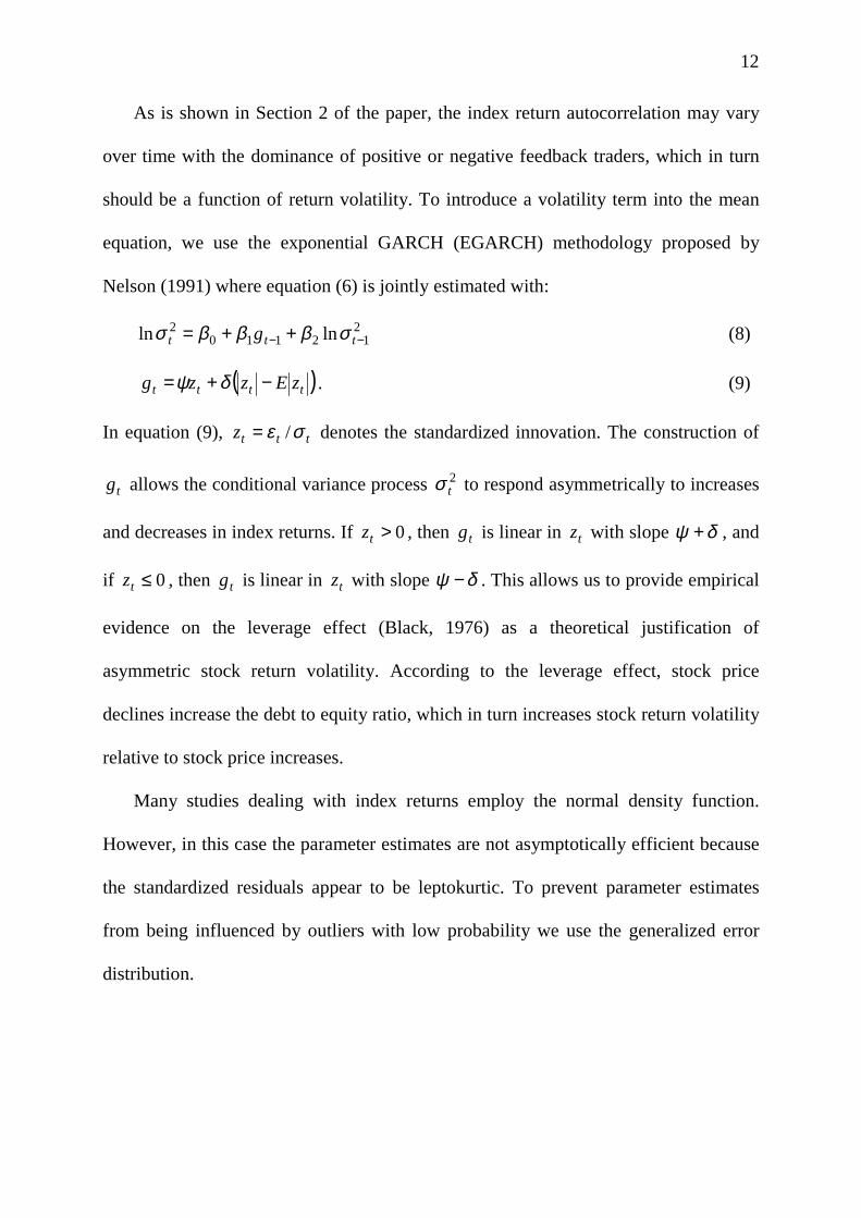
As is shown in Section 2 of the paper, the index return autocorrelation may vary

over time with the dominance of positive or negative feedback traders, which in turn

should be a function of return volatility. To introduce a volatility term into the mean

equation, we use the exponential GARCH (EGARCH) methodology proposed by

Nelson (1991) where equation (6) is jointly estimated with:

212110

2 lnln −− ++= ttt g σβββσ (8)

( )tttt zEzzg −+= δψ . (9)

In equation (9), tttz σε /= denotes the standardized innovation. The construction of

tg allows the conditional variance process 2tσ to respond asymmetrically to increases

and decreases in index returns. If 0>tz , then tg is linear in tz with slope δψ + , and

if 0≤tz , then tg is linear in tz with slope δψ − . This allows us to provide empirical

evidence on the leverage effect (Black, 1976) as a theoretical justification of

asymmetric stock return volatility. According to the leverage effect, stock price

declines increase the debt to equity ratio, which in turn increases stock return volatility

relative to stock price increases.

Many studies dealing with index returns employ the normal density function.

However, in this case the parameter estimates are not asymptotically efficient because

the standardized residuals appear to be leptokurtic. To prevent parameter estimates

from being influenced by outliers with low probability we use the generalized error

distribution.

13

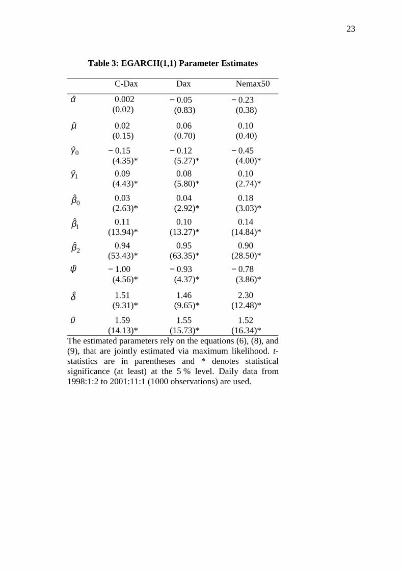
The estimation results are summarized in Table 3. The coefficients describing the

conditional variance process are statistically significant in all cases.2 When looking at

the estimates for ψ and δ there is evidence of asymmetry in the dependence of the

volatility from negative and positive innovations. The impact of negative innovations

is at least twice as large as the impact of positive innovations. This implies that in the

index returns under consideration the volatility is higher in periods of market decline

than in market upturns, which can be theoretically justified by the leverage effect. The

estimates of the 2β coefficients reveal a high degree of shock persistence in volatility.

Furthermore, the estimated model generates thick tails with both a randomly changing

conditional variance and a thick tailed conditional distribution for the standardized

errors. According to the values of υ̂ the distribution of the tε̂ is significantly thicker-

tailed than the normal distribution.

Table 3 about here

We now turn to the crucial findings of the parameter estimates 0γ̂ and 1γ̂ to

answer the question about the existence of positive feedback traders in the three

German stock market segments. The results are consistent with our theoretical

suggestions because all 0γ̂ coefficients are statistically significant negative and the 1γ̂

2 In addition to the EGARCH(1, 1) specification, we experimented with processes of

higher order. The coefficients of higher order processes are statistically insignificant

(results are not shown but available on request), which justifies the use of the

parsimonious EGARCH(1, 1) model.

14

parameters are significant positive. During periods of high volatility there is enough

positive feedback trading in the German stock market to produce negative first order

autocorrelated returns, even though other factors tend to generate positive

autocorrelation. These findings are broadly consistent with the empirical evidence in

Sentana and Wadhwani (1992), Koutmos (1997), and Koutmos and Said (2001) for

other developed, as well as, emerging stock markets.

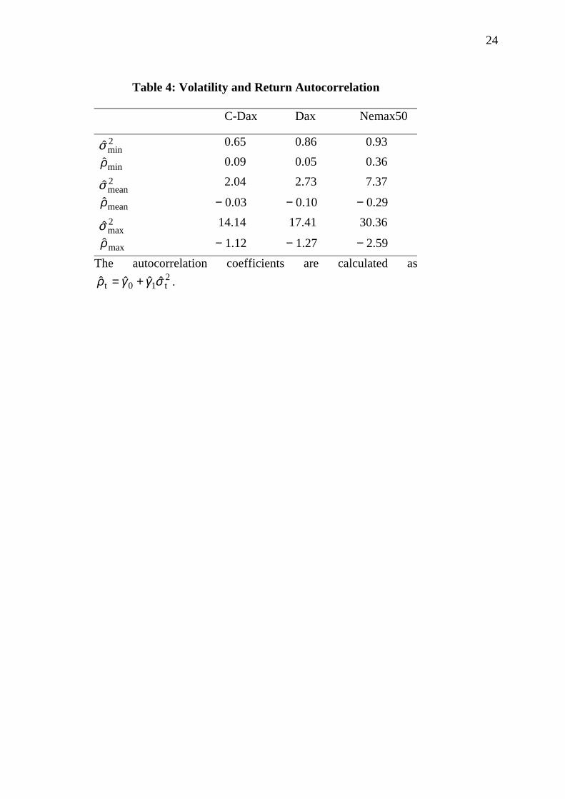
So far, the empirical results meet the necessary condition that the estimates for 0γ

and 1γ have the expected signs. But according to equation (6), stock index returns

only exhibit negative autocorrelation if the magnitude of a negative 1γ is sufficiently

high to compensate for a positive 0γ , given conditional return volatilities. Therefore,

we assess the empirical relevance of positive feedback trading by calculating the

autocorrelation coefficient, 2t10t ˆˆˆˆ σγγρ += , for the estimated minimum, mean, and

maximum conditional volatility. The results are reported in Table 4.

Table 4 about here

The calculated values minρ̂ , meanρ̂ , and maxρ̂ indicate that positive feedback trading

is not a phenomenon of a few trading days with peaking volatility, but can be found at

(fairly low) mean volatility levels. With increasing volatility positive feedback traders

have an even greater influence on the index returns inducing negative return

autocorrelation which confirms the theory suggested above.

15

4. Conclusion

In this paper we provide empirical evidence on the importance of positive

feedback trading for the return behavior in different German stock market segments.

Relying on the theoretical models put forward by Shiller (1984) and Sentana and

Wadhwani (1992) we use the link between index return autocorrelation and volatility

to better understand the return characteristics generated by traders adhering to positive

feedback trading strategies. Germany’s C-Dax, Dax, and Nemax50 indices for the

period from January 1, 1998 to November 1, 2001, represent different stock market

segments, thereby providing an interesting and broad platform for an analysis of

feedback trading strategies.

First, we provide empirical evidence relying on the stock market crash due to the

terrorist acts in the U.S. on September 11, 2001. Few economists will disagree that

volatility had enormously increased in the days after the stock price crash, which lead

directly to the question of the autocorrelation properties in returns during this turbulent

period. Our simple dummy variable approach exhibits empirical results that are

consistent with the theory regarding the relationship between volatility and

autocorrelation in index returns. Whereas index returns show shortly after the crash

strong negative autocorrelation indicating the existence of positive feedback traders,

the negative serial correlation in returns vanishes the week after the crash when

volatility has decreased.

The application of Nelson’s (1991) exponential GARCH model as a more

sophisticated approach relies on an explicit volatility measure and allows the

conditional variance to respond asymmetrically to positive and negative innovations.

Our findings provide strong support for the existence of a leverage effect. This implies

16

that in Germany’s C-Dax, Dax, and Nemax50 index volatility is higher in bearish

periods compared to bullish periods. More importantly and consistent with the

empirical results of the event study of the September 11 crash, our empirical evidence

shows that positive feedback traders are present in these stock market segments and

generate negative return autocorrelation even at mean levels of return volatility.

17

References

Bange, M. M. (2000), „Do the Portfolios of Small Investors Reflect Positive Feedback

Trading?”, Journal of Financial and Quantitative Analysis 35, 239 – 55.

Black, F. (1976), „Studies of Stock Volatility Changes”, Proceedings of the American

Statistical Association, Business and Economic Statistics Section, 177 – 81.

Boudoukh, J., Richardson, M. P. and M. P. Whitelaw (1994), „A Tale of Three

Schools: Insights on Autocorrelations of Short-Horizon Stock Returns, Review of

Financial Studies 7, 539 – 73.

Campbell, J. Y. and A. Kyle (1993), „Smart Money, Noise Trading, and Stock Price

Behavior“, Review of Economic Studies 60, 1 – 34.

Conrad, J. and G. Kaul (1988), „Time-Variation in Expected Returns“, Journal of

Business 61, 409 – 25.

Cutler, D. M, J. M. Poterba and L. H. Summers (1990), “Speculative Dynamics and

the Role of Feedback Traders”, American Economic Review, Papers and Proceedings

80, 63 – 8.

DeBondt, W. E. M. (1993), „Betting on Trends: Intuitive Forecasts of Financial Risk

and Return”, International Journal of Forecasting 9, 355 – 71.

18

DeLong, B. J., A. Shleifer, L. H. Summers and R. J. Waldmann (1990), „Noise Trader

Risk in Financial Markets“, Journal of Political Economy 98, 703 – 38.

Kirman, A. P. (1993), „Ants, Rationality, and Recruitment“, Quarterly Journal of

Economics 108, 137 – 56.

Koutmos, G. (1997), „Feedback Trading and the Autocorrelation Pattern in Stock

Returns: Further Empirical Evidence“, Journal of International Money and Finance

16, 625 – 36.

Koutmos, G. and R. Said (2001), „Positive Feedback Trading in Emerging Capital

Markets“, Applied Financial Economics 11, 291 – 97.

Kroll, Y., H. Levy and A. Rapoport (1888), „Empirical Tests of the Mean-Variance

Model for Portfolio Selection, Organizational Behavior and Human Decision

Processes 42, 388 – 410.

Lakonishok, J., A. Shleifer and R. W. Vishny (1992), „The Impact of Institutional

Trading on Stock Prices”, Journal of Financial Economics 32, 23 – 43.

Lo, A. and A. C. MacKinlay (1990), „An Econometric Analysis of Non-Synchronous

Trading,“ Journal of Econometrics 45, 181 – 212.

19

McQueen, G., M. Pinegar and S. Thorley (1996), „Delayed Reaction to Good News

and the Cross-Autocorelation of Portfolio Returns“, Journal of Finance 51, 889 – 919.

Mech, T. (1993), „Portfolio Return Autocorrelation“, Journal of Financial Economics

34, 307 – 44.

Merton, R. (1973), „An Intertemporal Capital Asset Pricing Model“, Econometrica 41,

867 – 88.

Nelson, D. (1991), „Conditional Heteroskedasticity in Stock Returns: A New

Approach”, Econometrica 59, 347 – 70.

Odean, T. (1998), „Are Investors Reluctant to Realize Their Losses?”, Journal of

Finance 53, 1775 – 98.

Ogden, J. P. (1997), „Empirical Analyses of Three Explanantions for the

Autocorrelation of Short-Horizon Stock Index Returns“, Review of Quantitative

Finance and Accounting 9, 203 – 17.

Sentana, E. and S. Wadhwani (1992), „Feedback Traders and Stock Return

Autocorrelations: Evidence from a Century of Daily Data“, The Economic Journal

102, 415 – 25.

20

Shefrin, H. and M. Statman (1985), „The Disposition to Sell Winners Too Early and

Ride Losers Too Long: Theory and Evidence”, Journal of Finance 40, 777 – 90.

Shiller, R. J. (1988), „Portfolio Insurance and Other Investor Fashions as Factors in the

1987 Stock Market Crash”, NBER Macroeconomic Annual, 287 – 96.

Shiller, R. J. (1984), „Stock Prices and Social Dynamics“, Brooking Papers on

Economic Activity 2, 457 – 98.

Shleifer, A. (2000), Inefficient Markets. An Introduction to Behavioral Finance,

Oxford University Press, Oxford.

21

Table 1: September 11 Crash and Autocorrelation in Stock Returns

Index Dummy Period α̂ 0γ̂ 1γ̂ 2R

C-Dax September 11 to 14 − 0.002 (0.05)

0.03 (0.06)

− 0.28* (2.82)

0.003

September 11 to 18 − 0.002 (0.04)

0.02 (0.06)

− 0.25* (2.69)

0.003

September 19 to 25 0.001 (0.02)

0.01 (0.25)

0.14 (0.51)

0.001

Dax September 11 to 14 0.002 (0.04)

0.003 (0.06)

− 0.31* (2.38)

0.004

September 11 to 18 0.003 (0.05)

0.002 (0.06)

− 0.28* (2.37)

0.004

September 19 to 25 0.01 (0.13)

− 0.02 (0.42)

0.19 (0.72)

0.001

Nemax50 September 11 to 14 0.001 (0.01)

0.14* (3.41)

− 0.28* (2.73)

0.02

September 11 to 18 0.001 (0.01)

0.14* (3.39)

− 0.23 (1.89)

0.02

September 19 to 25 0.003 (0.03)

− 0.13* (3.42)

− 0.07 (0.16)

0.02

The estimated parameters rely on the model tttt RCrashR εγγα +++= −110 )( .2R denotes the adjusted coefficient of determination. t-statistics in parentheses

are based on heteroskedastic-consistent standard errors. * denotes statisticalsignificance (at least) at the 5 % level. Daily data from 1998:1:2 to 2001:11:1(1000 observations) are used.

22

Table 2: Time Series Characteristics of Index Returns

C-Dax Dax Nemax50

Mean 0.002 (0.96)

0.008 (0.88)

0.004 (0.96)

Variance 2.09 2.81 7.48

Skewness − 0.51 (0.00)

− 0.50 (0.00)

− 0.06 (0.00)

Kurtosis 6.90 (0.00)

5.10 (0.00)

5.32 (0.00)

Index returns are calculated as 100)ln(ln 1 ⋅−= −ttt PPR , where

tP is the index at time t . P-values are in parantheses. Dailydata from 1998:1:2 to 2001:11:1 (1000 observations) are used.

23

Table 3: EGARCH(1,1) Parameter Estimates

C-Dax Dax Nemax50

α̂ 0.002 (0.02)

− 0.05 (0.83)

− 0.23 (0.38)

µ̂ 0.02 (0.15)

0.06 (0.70)

0.10 (0.40)

0γ̂ − 0.15 (4.35)*

− 0.12 (5.27)*

− 0.45 (4.00)*

1γ̂ 0.09 (4.43)*

0.08 (5.80)*

0.10 (2.74)*

0β̂ 0.03 (2.63)*

0.04 (2.92)*

0.18 (3.03)*

1β̂ 0.11(13.94)*

0.10(13.27)*

0.14(14.84)*

2β̂ 0.94(53.43)*

0.95(63.35)*

0.90(28.50)*

ψ̂ − 1.00 (4.56)*

− 0.93 (4.37)*

− 0.78 (3.86)*

δ̂ 1.51 (9.31)*

1.46 (9.65)*

2.30(12.48)*

υ̂ 1.59(14.13)*

1.55(15.73)*

1.52(16.34)*

The estimated parameters rely on the equations (6), (8), and(9), that are jointly estimated via maximum likelihood. t-statistics are in parentheses and * denotes statisticalsignificance (at least) at the 5 % level. Daily data from1998:1:2 to 2001:11:1 (1000 observations) are used.

24

Table 4: Volatility and Return Autocorrelation

C-Dax Dax Nemax50

2minσ̂minρ̂

0.65 0.09

0.86 0.05

0.93 0.36

2meanσ̂meanρ̂

2.04

− 0.03

2.73

− 0.10

7.37

− 0.292maxσ̂maxρ̂

14.14

− 1.12

17.41

− 1.27

30.36

− 2.59The autocorrelation coefficients are calculated as

2t10t ˆˆˆˆ σγγρ += .