THE INFLUENCE OF MAUNA LOA OBSERVATORYON THE DEVELOPMENT OF ATMOSPHERIC CO2

RESEARCH

Charles D.. KeelingScripps Institution of OceanographyUniversity of Califorrlia at San Diego

INTRODUCTION

The increasing amount of CO2 in the atmosphere from the burning offossil fuels has become a serious environmental concern. Central to thisconcern is the question whether a rise in CO2 constitutes a peril to man byraising world temperatures, as many scientists now claim. That a rise in CO2

is occurring is unquestionable, however. Mauna Loa Observatory (MLO) dataare providing dramatic evidence of that: they ·show amounts more than 100/0over amounts recorded before the Industrial Revolution, and a rise of 6% inthe last 19 years alone.

Ninety-seven percent of the energy demand of the industrial world is mettoday by burning fossil fuels. Even if the industrialized world were to decideto shift to other energy sources as rapidly as possible, the annual consumptionof fossil fuels would double before the shift was complete. Without such ashift, a peak annual rate ten or even twenty times today's rate may occurbefore fuel reserves, especially coal reserves, are exhausted. Thus a large addi­tional increase in atmospheric CO2 is likely in the next few decades. AsRevelle and Suess (1957) wrote, "Through his worldwide industrialized civil­ization, man is unwittingly conducting a vast geophysical experiment. Withina few generations he is burning the fossil fuels that slowly accumulated in theearth over the past 500 million years."

The idea that CO2 from fossil fuel burning might accumulate in air andcause a warming of the lower atmosphere was speculated upon as early as thelatter half of the nineteenth century (Arrhenius, 1903). At that time the use of

36

fossil fuel was too slight to expect a rise in atmospheric CO2 to be detectable.The idea was again convincingly expressed by Callendar (1938, 1940) but stillwi thou t solid evidence of a rise in CO2 ,

The first unmistakable evidence of atmospheric CO2 increase wasfurnished by continuous measurements made at MLO and by ~easurementsofflask samples collected periodically at the South Pole. These data, obtained inconnection with the International Geophysical Year (ICY), were precise enoughto indicate a rise in concentration in 1959 when compared with the results ofthe previous year (Keeling, 1960). Further measurements have shown a persist­ent year-to-year increase.

Along with new observations have come increasingly refined calculationsof the heating effect of increased atmospheric CO2 , One of the most widelyaccepted climate models emerging from this effort indicates that the earth'ssurface would warm by 4°C above the present average global temperature fora fourfold increase in CO2 , by 6°C for an eightfold increase (GeophysicsStudy Committee, 1977). A rise in CO2 as great as eightfold before coalreserves are exhausted has been predicted using a geochemical model cali­brated by the Mauna Loa and South Pole trends (Keeling and Bacastow,1977).

Such a high average global temperature has probably not occurred fortens of millions of years. Accompanying such warming may be shifts inrainfall patterns and in agricultural zones. Polar ice may melt or break up andlead to coastal flooding (Geophysics Study Committee, 1977). These problems,once upon us, will not be easily overcome. Once high CO2 levels are reached,they will probably decrease only slowly as deep ocean water gradually absorbsthe excess CO2 • Concentrations well above preindustrial levels are likely topersist for at least 1,000 years, along with attending climatic problems (Keelingand Bacastow, 1977).

Whether or not a large CO2 increase will occur and persist depends on thenatural carbon cycle, about which we still know too little. How much CO2

from fossil fuel will remain in the air during the next centuries? How muchwill be taken up by the oceans and by vegetation on land? These questionscannot be answered from present knowledge. Sustained monitoring of CO2 atsites such as MLO is an indispensable aid to validate predictions stemming fromcalculations of the behavior of the carbon cycle.

Viewed in this context, the reasons for measuring atmospheric CO2 atMauna Loa seem compelling. A few of us remember, however, that theoriginal decision to study CO2 at this remote site was not easily made. Becausethe story is closely involved with MLO being established in the first place, itseems appropriate to recount here some of the human aspects of this story andits scientific perspective.

HISTORY

The ICY, which began in 1957, offered scientists for the first time an or­ganizational setting for study of atmospheric CO2 on a global scale. In view ofthe importance of knowing whether airborne CO2 was rising worldwide, sucha study was long overdue. The data published before the IGY led to a generalbelief that CO2 concentrations depended greatly on location with no clear timetrend (Bray, 1959). Observations varied from under 200 parts per million(ppm) near the North Pole to over 350 ppm in continental air and air near theequator (Buch, 1948). Owing to this apparent spatial variability, a wholenetwork of stations was deemed necessary to detect any significant globaltrend.

In the early 1950's, Carl G. Rossby suggested that Stockholm University'sMeteorological Institute, which he directed, should participate in an extensiveinvestigation of trace chemicals in the atmosphere as a prelude to the ICY. At aconference held on the subject in 1954, participants decided to plan for aworldwide network of CO2 monitoring stations, possibly including a site inthe Hawaiian islands (Eriksson, 1954). Responsibility for setting up stations inthe Pacific region fell to Wendel Mordy, a conference member and chiefmeteorologist of the Pineapple Research Institute in Honolulu.

When I learned that Mordy was interested in measuring atmospheric CO2

in the Pacific region, I informed him of CO2 studies I had begun in 1955 whileat the California Institute of Technology. In contrast to previous studies, I hadfound practically constant atmospheric CO2 in turbulent air near midday.

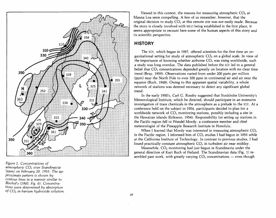
Meanwhile, CO2 monitoring had just begun in Scandinavia under thegeneral direction of Kurt Buch of Finland. The Scandinavian data (Fig. 1) re­sembled past work, with greatly varying CO2 concentrations - even though

Figure 1. Concentrations ofatmospheric CO2 over Scandinavia(ppm) on February 20, 1955. The ap­proximate pattern is shown bycontour lines in a manner similar toBischof's (1960, Fig. 6). Concentra­tions were determined by absorptionof CO2 in barium hydroxide solution.

37

special care was being taken to sample in open areas away from local in­fluences (Fonselius et al., 1955). My daytime CO2 results were close to theScandinavian means, but the variability was far less - even though I hadtaken special care to sample in densely vegetated areas /where local influenceswould predominate. Specifically, I had found that everywhere I went the air afew tens of meters from the plants on sunny days tended to reach a nearly'constant CO2 level of about 315 ppm (Keeling, 1958). In an attempt to under­stand why, I took measurements in some exposed windy areas away fromplants: at high elevation in the White Mountains (Fig. 2) and Sierra Nevada ofCalifornia, on ocean beaches, and over ocean water near the equator (Keeling,1961). All these data were also near 315 ppm. I concluded that the CO2 in airhad a characteristic background concentration, at least near the west coast ofthe United States and Central America where I had sampled. Evidently, onsunny days this background level prevailed even near plants.

Thus I became concerned that the proposed measurements in Hawaii andelsewhere might not be accurate enough to establish this background CO2

level. Although Mordy soon decided not to participate in CO2 studies, myconcerns reached the attention of Harry Wexler, Director of Research for theU.S. Weather Bureau. Wexler was a friend of Rossby and an ardent supporterof broadly based meteorological studies. He invited me to Washington early in1956.

The Weather Bureau already had a small wood frame hut near thesummit of Mauna Loa where some simple automatic instruments were housed.In 1955, at Wexler's urging, plans were underway to construct a larger, morepermanent structure where people would live and tend more complicated in­struments. During my interview with Wexler, which I recall began promptly at8:00 a.m., I talked to him about the possibility of setting up a continuous

recording CO2 gas analyzer on Mauna Loa since it would be possible to livethere and tend the analyzer as necessary. As far as I knew, no one had everbefore suggested measuring atmospheric CO2 continuously. Wexler asked anumber of questions in rapid-fire, covering both the scientific and the prac­tical. He was especially interested in costs. We went so far as to discuss settingup a second continuous CO2 analyzer in Antarctica. Then the interview wasover. Altogether it took almost exactly 15 minutes, as scheduled. Wexler hadmade up his mind to press for CO2 measurements at Mauna Loa using monieswhich he hoped would be made available by the participation of the UnitedStates in the ICY.

During this same spring of 1956 the oceanographic community wasmaking plans to participate in the ICY. Roger Revelle, as director of theScripps Institution of Oceanography, was a leader in this effort. Revelle hadan intimate knowledge of the natural CO2 cycle going back to his studentdays, and he wanted to make sure that man's "vast geophysical experiment"would be properly monitored and its results analyzed. Revelle believed that aCO2 program should include ocean water studies as well as atmosphericmeasurements. With this in mind and with Wexler's concurrence, he arrangedfunding for a laboratory for CO2 measurements at Scripps, and I was invitedto run it. Although it had not been decided precisely what kind of CO2

program should be implemented as part of the United States ICY effort, Iaccepted his offer.

Wexler's support of continuous measurements of atmospheric CO2 at MLO

was a bold decision not Widely accepted at the time. Wexler knew that I hadlocated a manufacturer of nondispersive infrared CO2 gas analyzers, but healso knew that I had not yet been able to test such an analyzer. Even the firmitself did not claim that its infrared analyzer was accurate enough for the task.

320 .------r----r----,---..-- r---~--~--.._-~--....,...._-__,

..131211

March 1956

109315 ----~--~--..L...-_ ___a..._____L...__....l..__ _J__~__..L__ ___L._ __._J.

14

38

It had been designed principally for industrial uses which did not demand highaccuracy. I was relying on the judgment of one of the firm's engineers that thedevice was inherently very sensitive and stable. The firm couldn't even lendme one to test. The basic instrument was expensive and required costly addi­tional equipment to operate as an air monitor at a remote field station. Refer­ence gases to calibrate the instrument did not exist.

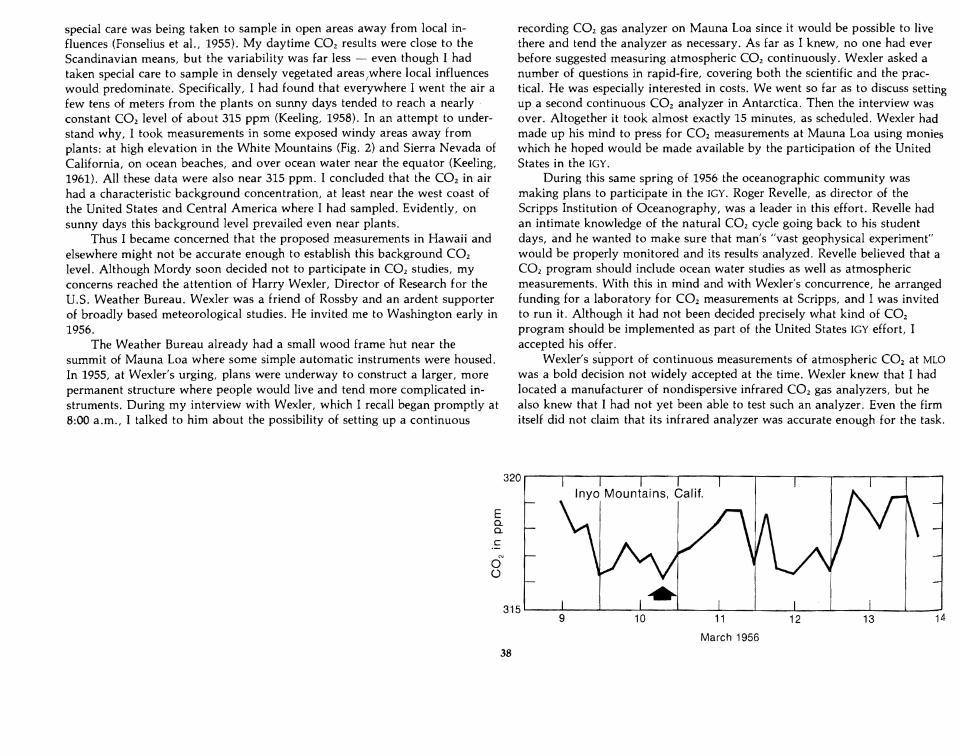
To most of the IGY planners who heard about the CO2 infrared analyzerscheme in 1956, such expensive and complicated equipment seemed unneces­sary. Both the earlier published data and the new Scandinavian data, appear­ing in print every 3 months, proved that atmospheric CO2 variations were solarge that traditional methods of chemical analysis would always remain ade­quate. I distrusted these variable data, but my distrust was based on no morethan a few hints from my own data. The most important of these was the nearconstancy of CO2 over five days for samples taken at 3,500 m in the WhiteMountains. Wexler had been especially impressed by the White Mountainsrecord (reproduced in Fig. 2). He felt that if this record was typical of back­ground air, high measurement accuracy at a site on Mauna Loa just might payoff in the IGY program.

Revelle soon agreed to the new infrared analyzer method, but he preferreda network of measuring locations in which such analyzers would be used toanalyze air collected in flasks, from ships and aircraft for example.

Rossby remained dubious. I had a chance to meet him just once at an IGY

planning meeting at Scripps during 1956. Som~one pointed me out to himacross a grass lawn during a recess. As he walked up to greet me, he remarkedfor the benefit of some nearby acquaintances, "Ah ... za yong man wiz zamachine." He seemed upset at this abrupt new American plan to buyexpensive gadgetry to measure CO2 • His skepticism became obvious as we

Figure 2. Variation in atmosphericCO2 over barren ground near WhiteMountain Research Station in theInyo Mountains of California duringMarch 1956 (adapted from Fig. 2 ofKeeling, 1961). Concentrations weredetermined manometrically fromliquid nitrogen temperaturecondensates. The arrow identifies theminimum concentration plotted inFig. 4, accepted as representative ofWest coast U. S. air.

39

talked about plans for an ambitious instrument-based United States program.Ironically, I had so far obtained CO2 data using quite inexpensive devices

- glass sampling flasks, a liquid nitrogen cooled freeze-out trap, a mercurycolumn manometer. But my manometric method could not be used for a largeprogram because a single sample took over an hour to analyze. The infraredgas analyzer was needed to speed up the work without sacrificing high ac­curacy.

Late in the summer of 1956 I arrived at Scripps to begin implementing thenew U.S. atmospheric CO2 program. In all, four gas analyzers were pur­chased. One was hastily outfitted for Antarctic field work. Shipment to LittleAmerica couldn't be delayed. This first venture turned out, in fact, to be toohasty. No useful data were obtained at Little America until the second Ant­arctic field year in 1958.

As soon as the Antarctic shipment was off - on the same'vessel that wasto have carried Admiral Byrd to Antarctica, had he been able to go - I begansystematically to test the new analyzers. In March 1957, continuous measure­ments of air began at Scripps. Soon afterward I assembled another apparatusfor Mauna Loa. But there were numerous delays and problems with the air­craft and shipboard programs. These delays were especially bothersomebecause the IGY had already begun. Soon it would be over, and ships and air­craft would not be available.

As it turned out, when the equipment for Mauna Loa was ready, Icouldn't install it. Revelle insisted that I give first attention to aircraft andshipboard sampling, and the aircraft program was not yet underway. He rein­forced his view of the matter by refraining from signing my travel orders tovisit Mauna Loa. As the IGY approached its July 1958 ending date, Wexlerbecame very anxious about Mauna Loa. At length he took action himself and

sent to me Ben Harlin, the meteorologist who had operated the CO2

equipment at Little America in 1957. With help from Jack Pales, the firstdirector of MLO, Harlin installed the analyzer at MLO in March 1958 withoutmy assistance. To our great surprise, on the first day of operation it deliveredwithin 1 ppm the CO2 concentration that I had told Harlin to expect on thebasis of my earlier manometric data and preliminary test data obtained atScripps.

Of course this agreement was an accident. The mean of the daytimemanometric and Scripps data just happened to be close to the value typical forthe month of March. Indeed, the next month's data did not agree - the con­centration rose by over one ppm. The following month's mean concentrationwas still higher. Electrical power failures then shut down the equipment forseveral weeks. When measuring resumed in July, the concentration had fallenbelow the March value. I became anxious that the concentration was going tobe hopelessly erratic, especially when the computed concentration fell again inlate August. Then there were more power shutdowns.

Finally, after my first visit to Mauna Loa in November, the concentrationstarted to climb steadily month by month. Gradually a regular seasonalpattern began to emerge: we were witnessing for the first time nature'sborrowing of CO2 for plant growth during the summer and returning the loaneach succeeding winter. Earlier published data for Europe also showed aseasonal trend of sorts (Bray, 1959), but the maximum concentration, arrivedat statistically from a highly irregular pattern, was in January, a time of yearwhen CO2 from burning is likely to accumulate near the ground because of

b

336

332

328Ec-o..~ 324ON0

320

316

3121960 1965

year1970 1975

40

winter temperature inversions. The maximum at Mauna Loa occurred in Mayjust before temperate and boreal plants add new leaves. The seasonal patternwas highly regular and almost exactly repeated itself during the second year ofmeasurements at Mauna Loa. Thus there was no need to wait for statisticalstudies to prove the reality of the oscillation as would have been required hadless exact chemical methods been used. I soon reviewed my 1955-1956manometric data and discovered that they showed a similar seasonal variation(Bolin and Keeling, 1963).

No one had expected to determine the long-term rate of rise in CO2

during the ICY even though establishing the rise was the principal purpose ofthe program. Revelle and others had expected that the ICY program at bestwould furnish a reliable IIbaseline" CO2 level which could be checked 10 or 20years later, after the rise in CO2 was large enough to stand out against localvariability. But because of the regularity of the seasonal variation at MaunaLoa a rough estimate of the long-term rise was possible after only two years(Bolin and Keeling, 1963).

Fortunately, funding for CO2 measurements at MLO was continued afterthe ICY. By early 1962 it was possible to deduce that approximately half of theCO2 from fossil fuel was accumulating in the air and that a sink must becarrying a substantial fraction away (Keeling, 1960). Revelle and Suess (1957)had predicted that much .of the CO2 from fossil fuel would be absorbed by theoceans. The earlier published CO2 data had argued against their view,however, because the rise in CO2 seemed to be close to that predicted if all ofthe CO2 from fossil fuel accumulated in the air. This latter conclusion wasreinforced in 1958 after several years of the Scandinavian network databecame available (Callendar, 1958). But after four years of measurement atMauna Loa the question was settled in favor of the Revelle-Suess prediction.

Figure 3. Monthly averageconcentrations of atmospheric CO2 atMLG since the beginning ofmonitoring in 1958. Concentrationswere determined with a nondispersiveinfrared gas analyzer as described byKeeling et al. (1976a), p. 539.

As the Mauna Loa record has been further extended, additional interestingfeatures of the long-term trend have revealed themselves. These include pertur­bations that appear to correlate with the trade winds and with sea surface tem­perature (Bacastow, 1976; Machta et al., 1976; Newell and Weare, 1977). Theseasonal pattern has also been scrutinized to see if variations in amplitudefrom year to year are meaningful. So far the pattern is too regular to revealsignificant variations (Hall et al., 1975). Now after nearly 20 years of measure­ments, the Mauna Loa record (Fig. 3) appears as a natural yearly cycle gradu­ally being dwarfed by a long-term rise - a dramatic example of inadvertentinfluence by man on his environment.

THE WEST COAST DATAEven though the manometric CO2 data obtained shortly before the ICY

played a prominent role in deciding the strategy of the United States CO2

program, they had never been compared with the infrared CO2 data forMauna Loa. Until a pressure broadening correction was recently applied to thelatter data (Keeling et al., 1976a), a precise comparison was not possible. Itseems worthwhile now to review these earlier measurements and to recon­struct, as closely as possible, the global concentrations of CO2 back to 1955.

This reconstruction is greatly aided by additional infrared measurementsof CO2 obtained between 1957 and 1962 at La Jolla, California. Althoughthese data were obtained as a by-product of instrument testing, they are never­theless a useful record of air from the same general geographic area as theearlier manometric data. Except for a few days when air was sampled from alaboratory window, all measurements were made near the end of a 1,000-footocean pier where the air was often free of local disturbances, at least during

sea breezes. The CO2 record was twice interrupted for several months whenoceanographic work was in progress, but a nearly unbroken continuous recordexists from April 1958 to June 1960. Since the Mauna Loa analyzer was op­erating during this period, these data, and a few more in 1962, are useful inadjusting the La Jolla record to a common basis with Mauna Loa.

Most of the 1955-1956 manometric data reflect local CO2 emanating fromplants and soil. The minimum values for each location, occurring typicallynear midday, as already noted, may not have been markedly influenced byplant activity, however. A plausible reason for this is that the sampling loca­tions I had chosen were in wild areas which had never been disturbed verymuch by humans. In wild areas the photosynthetic withdrawal of atmosphericCO2 by the plants and the release of CO2 by plant respiration and decomposi­tion should not differ greatly. The net change in the CO2 concentration of thelocal air should therefore be relatively small, especially if air turbulence,typically maximal at midday, further diminishes the net effect.

At several control sites on ocean beaches and barren mountains, where Ialso sampled during 1955 and 1956, the CO2 concentrations usually agreedwith the minimum values found near plants. For example, in YosemiteNational Park in June 1955, the lowest value found for forest air was 316.2ppm; a few miles away over barren terrain near Lake Tenaya, I found 315.9ppm (Eriksson, 1954).

The minimum CO2 concentrations for all CO2 sites in the western UnitedStates are listed in Table 1 and plotted in Fig. 4, except that data have beenomitted if the humidity was not measured, since for these data it is impossibleto determine the CO2 concentration versus dry air. Most of the measurementswere obtained in California, but a few were obtained farther north in the stateof Washington and several from Arizona.

41

Table 1. Minimum atmospheric carbon dioxide concentrations (relativeto dry air) by direct manometric analysis, for various sites near thewest coast of the United States and Central America

*Adjusted to 33 oN.

42

Also, as a single exception to the above site distribution, Table 1 includesthe minimum CO2 concentration from a suite of samples collected aboard shipoff the coast of Nicaragua near 9°N, in 1955. This minimum has been adjustedupward by 0.5 ppm on the basis of the average latitudinal gradient found byBolin and Keeling (1963) between 9 0 and 33 oN for the appropriate month ofsampling.

The continuous measurements obtained at La Jolla from 1957 to 1962 arehighly contaminated by local and regional urban sources of CO2 • Even thedaily minima, which usually occurred during sea breezes, vary considerablydepending on the history of the air. Highest values typically occurred whenthe air had previously passed near the city of Los Angeles to the northwest.To reduce further the influence of contamination, the daily minima were ar­ranged into calendar weeks, and weekly minima were identified. As notedalready in 1960 (Keeling, 1961), these weekly minima scatter much less thanthe dailies. Also, unlike the dailies their monthly means show a consistenttrend suggestive of uncontaminated air.

These monthly means are listed in Table 2 and plotted in Fig. 5. Oneentry, for June 1958, is omitted from further consideration because only oneweekly minimum was obtained that month. Also, as indicated in the table, afew obviously contaminated minima were omitted in assembling the monthlymeans. The means for April 1958 through March 1960 have been published(Keeling, 1961). These, and previously unpublished data for 1957, 1960, and1962, are here reported according to the 1974 manometric CO2 mole fractionscale, using formulas for conversion from an adjusted index scale (Keeling etal.,1976a).

The manometric and infrared data (Figs. 4 and 5) display a seasonalvariation similar to but of greater amplitude than that for Mauna Loa. The

Figure 4. Minimum concentrations ofatmospheric CO2 at various sites nearthe west coast of the United Statesduring 1955 and 1956. Concentrationsu:ere determined manometrically fromlIquid nitrogen temperature conden­sates. Sites are identified as follows:

BS, Big Sur; YF, Yosemite forest; YB,Yosemite barren ground; OF,Olympic forest; OB, Olympic beach;GT, Gulf of Tehuantepec; BV,Borrego Valley; 1M, Inyo Mountains;OP, Organ Pipe; HP, HowardPocket; TH, Telephone Hill.

43

Table 2. Mean of weekly minimum concentration of atmospheric carbondioxide (relative to dry air) by infrared gas analysis, for Scripps pier,La Jolla, California, at 33°N, 117°W, elevation 8 m

Figure 5. Monthly averages of theweekly minimum atmospheric CO2

concentration at La Jolla, California.Concentrations were determined witha nondispersive infrared gas analyzer.

1

310~__i----L. ---J.... ~ ....I...--_-_--..J __

320

Ea.a.c

*One weekly minimum omitted from average.

1957 1958 1959 1960 1961 1962

44

X(t) = Ql sin 27ft + Q2 cos 27ft + Q3 sin 47ft + (1)Q4 cos 47ft + Qs + Q6t

The four possibly contaminated data mentioned above were tentativelyomitted from the computation. The parameters of best fit were found to havethe values:

seasonal variation, however, is clearly evident only for the La Jolla databecause the 1955-1956 manometric data involve so many missing months andextend over less than two years.

Several of the manometric data appear to be inconsistent with theseasonal trend. That the two CO2 minima for Big Sur State Park may be toohigh, both in 1955 and 1956, is not surprising because sampling was done in apublic campground where daytime automobile traffic may have producedseveral ppm of contamination. Also, the CO2 minimum for Telephone Hill,Arizona, seems too high relative to Howard Pocket, but there is no obviousreason, since the site was in a remote forest north of the Grand Canyon.Finally, the pair of CO2 minima for the Olympic National Park agree witheach other but are both considerably higher than had been expected for themonth of sampling on the basis of the La Jolla data, again for no obviousreason.

Before deciding on the disposition of these possibly contaminated values,an adjustment of the data was made to the 15th of the month of sampling inorder to reduce scatter resulting from uneven spacing in time. The adjustmentswere made following a procedure described previously (Keeling et al., 1976b).Specifically, the individual monthly concentrations X(t), in ppm, where t de­notes the time in years after January 1, 1955, were fit by the method of leastsquares to an oscillatory-linear trend function:

(2)Q4 = 6.64806 ppmQs = 312.684 ppmQ6 = 0.6954 ppm yr-1

2.86883 ppm0.879716 ppm

-1.51123 ppm

On the basis of equations (1) and (2), the data, including the tentativelyrejected values, were adjusted to the 15th of the month as listed in Tables 3and 4. Next, the data were seasonally adjusted using the first four terms of

*Judged to be contaminated.

Table 3. Adjusted manometric data, 1955-1956, and infrared gas analyzerdata, 1957

45

Table 4. Comparison of atmospheric carbon dioxide concentrations atLa Jolla with the long-term trend in concentration at MLO

*Adjusted to the 15th of the month.* *Determined for the 15th of the month from a spline fit of the seasonally adjusted monthly

means for 1958-1976, inclusive.

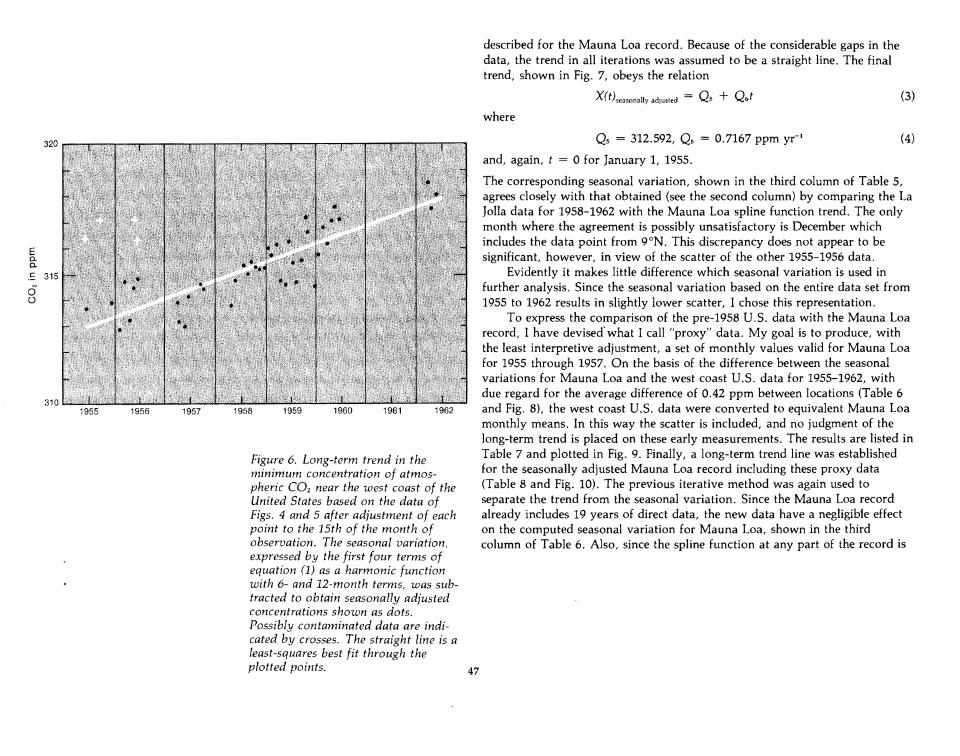
equation (1), and the resulting trend data were plotted as shown in Fig. 6.From this plot it becomes clear that the questionable values, shown as crosses,should be rejected. A statistical computation bears this out: the four valuesdiffer by factors of 3.4 to 4.9 times the root mean square departure of theremaining 13 data points for 1955-1957 with respect to equations (1) and (2).

The next step was to establish from overlapping data the difference inseasonal variation and long-term trend for Mauna Loa and La Jolla. First,from the entire Mauna Loa'record of monthly averages from March 1958through December 1976, the average seasonal variation and seasonally ad­justed trend for that station were established.

Several methods have been used previously to separate the long-termtrend at Mauna Loa from the associated seasonal variation (Bacastow, 1977).Here I have chosen to express the trend by a cubic spline function (Reinsch,1967) and the seasonal variation as an average of the monthly meanconcentrations after subtracting the trend. Since the two features are notuniquely separable, an iterative procedure was used. First, an estimate of thelong-term trend was found assuming a linear increase with time, and a prelimi­nary estimate of the seasonal variation was obtained. Then consistent with thisseasonal variation, the original monthly values were seasonally adjusted, anda cubic spline function was passed through the adjusted data points. Furtheriterations were carried out until the adjusted values approached constancy.This convergence was rapid, and because of the high regularity of the seasonalvariation, the seasonal variation found was similar to that found by using aleast squares fit based on equation (1).

Next, as shown in Table 4, the long-term trend for Mauna Loa, expressedas a spline function, was compared with the La Jolla data adjusted to the 15thof each month. For the relatively short period of the comparison it seemsreasonable to assume that the long-term trends for Mauna Loa and La Jolladiffer by only a constant. On the basis of the monthly differences between theMauna Loa trend and the La Jolla data (last column of Table 4), mean differ­ences between stations were determined for each month. The sum of these dif­ferences is -0.42 ppm; that is, the La Jolla weekly minima, on average, arelower by that amount than the Mauna Loa trend. Since the expected latitu­dinal difference between stations according to aircraft and shipboard dataanalyzed by Bolin and Keeling (1963) is -0.20 ppm, the weekly minima agreeclosely with expectations in spite of the high degree of selection involved inobtaining them. Evidently, the large irregular variations in the original La Jollarecord are almost solely owing to high values, probably produced by urbansources.

Next, from the west coast data, 1955-1962, a long-term trend and anaverage seasonal variation were found in the same manner as that just

46

described for the Mauna Loa record. Because of the considerable gaps in thedata, the trend in all iterations was assumed to be a straight line. The finaltrend, shown in Fig. 7, obeys the relation

x(t) seasonally adjusted = Qs + Q6 t

where

(3)

Figure 6. Long-term trend in theminimum concentration of atmos­pheric CO2 near the west coast of theUnited States based on the data ofFigs. 4 and 5 after adjustment of eachpoint to the 15th of the month ofobservation. The seasonal variation,expressed by the first four terms ofequation (1) as a harmonic functionwith 6- and 12-month terms, was sub­tracted to obtain seasonally adjustedconcentrations shown as dots.Possibly contaminated data are indi­cated by crosses. The straight line is aleast-squares best fit through theplotted points.

(4)320

E0.0.

c:: 315

o()

3101955 1956 1957 1958 1959 1960 1961 1962

47

Qs = 312.592, Q6 = 0.7167 ppm yr-1

and, again, t = 0 for January 1, 1955.

The corresponding seasonal variation, shown in the third column of Table 5,agrees closely with that obtained (see the second column) by comparing the LaJolla data for 1958-1962 with the Mauna Loa spline function trend. The onlymonth where the agreement is possibly unsatisfactory is December whichincludes the data point from 9oN. This discrepancy does not appear to besignificant, however, in view of the scatter of the other 1955-1956 data.

Evidently it makes little difference which seasonal variation is used infurther analysis. Since the seasonal variation based on the entire data set from1955 to 1962 resul ts in slightly lower scatter, I chose this representation.

To express the comparison of the pre-1958 U.S. data with the Mauna Loarecord, I have devised' what I call IIproxy" data. My goal is to produce, withthe least interpretive adjustment, a set of monthly values valid for Mauna Loafor 1955 through 1957. On the basis of the difference between the seasonalvariations for Mauna Loa and the west coast U.S. data for 1955-1962, withdue regard for the average difference of 0.42 ppm between locations (Table 6and Fig. 8), the west coast U.S. data were converted to equivalent Mauna Loamonthly means. In this way the scatter is included, and no judgment of thelong-term trend is placed on these early measurements. The results are listed inTable 7 and plotted in Fig. 9. Finally, a long-term trend line was establishedfor the seasonally adjusted Mauna Loa record including these proxy data(Table 8 and Fig. 10). The previous iterative method was again used toseparate the trend from the seasonal variation. Since the Mauna Loa recordalready includes 19 years of direct data, the new data have a negligible effecton the computed seasonal variation for Mauna Loa, shown in the thirdcolumn of Table 6. Also, since the spline function at any part of the record is

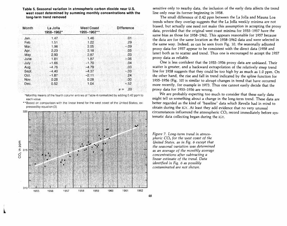
Table 5. Seasonal variation in atmospheric carbon dioxide near U.S.west coast determined by summing monthly concentrations with thelong-term trend removed

Figure 7. Long-term trend in atmos­pheric CO2 for the west coast of theUnited States, as in Fig. 6 except thatthe seasonal variation was determinedas an average of the monthly averageconcentrations after subtracting alinear estimate of the trend. Dataidentified in Fig. 6 as possiblycontaminated are not shown.

sensitive only to nearby data, the inclusion of the early data affects the trendline only near its former beginning in 1958.

The small difference of 0.42 ppm between the La Jolla and Mauna Loatrends where they overlap suggests that 'the La Jolla weekly minima are notbiased, but actually one need not make this assumption in accepting the proxydata, provided that the original west coast minima for 1955-1957 have thesame bias as those for 1958-1962. This appears reasonable for 1957 becausethe data are for the same location as the 1958-1962 data and were selected inthe same way. Indeed, as can be seen from Fig. 10, the seasonally adjustedproxy data for 1957 appear to be consistent with the direct data (1958 andlater) both as to scatter and trend. Thus one is encouraged to accept the 1957proxy data as reliable.

One is less confident that the 1955-1956 proxy data are unbiased. Theirscatter is greater, and a backward extrapolation of the relatively steep trendline for 1958 suggests that they could be too high by as much as 1.0 ppm. Onthe other hand, the rise and fall in trend indicated by the spline function for1955-1956 (Fig. 10) is similar to abrupt changes in trend that have occurredmore recently, for example in 1973. Thus one cannot easily decide that theproxy data for 1955-1956 are wrong.

We are probably expecting too much to consider that these early datamight tell us something about a change in the long-term trend. These data arebetter regarded as the kind of "baseline" data which Revelle had in mind toobtain during the ICY. At least they add evidence that no very unusualcircumstances influenced the atmospheric CO2 record immediately before sys­tematic data collecting began during the ICY.

19621961196019591958195719561955310

* Monthly means of the fourth column entries of Table 4 normalized by adding 0.42 ppm toeach value.

* * Based on comparison with the linear trend for the west coast of the United States, ex­pressed by equation (3).

320

EQ.Q.

.~ 315

o()

48

Table 6. Seasonal variation in atmospheric carbon dioxide - compari­son of west coast United States, 1955-1962, with MLO, 1958-1975

*Third column of Table 5 reduced by 0.42 ppm.

6

+

\-+6 12

Month

E0.0.C

~ +..........:::J

~ 0 'I--~t...-------+-+-~------.ja-:--+--.....,e...---------t0.0,)

oo()

Figure 8. Atmospheric CO2 as afunction of the month of the yeardetermined as a departure of themonthly mean concentration from thelong-term trend for Mauna Loa. Dataare shown for MLO by dots, and forthe west coast of the United States bycrosses. Months 1 to 6 (Januarythrough June) are plotted twice toreveal the seasonal patterns morefully.

49

Figure 9. Trend in atmospheric CO2

concentrations at MLD. The dotsindicate the monthly average concen­tration. Data in 1955, 1956, and 1957are proxy data based on observationsfor the west coast of the UnitedStates. The oscillatory curoe is aspline fit of the sum of the long-termtrend and the average seasonal varia­tion determined as in Fig. 7.

Table 7. Monthly average concentration of atmospheric carbon dioxide(ppm) at MLO expressed according to the 1974 manometric molefraction scale

330

[ 3250­

c

315

31 a 1o----.........~__'_..........L___L_.L...._...L...-.....1...._.L............--L____JL._.L....._...J.........J....__l...____L_.JL_.L...._....L.__L.____..l..............1.____Jl___J

1954 1956 1958 1960 1962 1964 1966 1968 1970 1972 1974 1976 1978

Year

*Proxy data.

50

Figure 10. Long-term trend in atmos­pheric CO2 concentration at MLG.The plot is the same as Fig. 9 exceptthat the seasonal variation has beensubtracted out.

330

0'"

8320

315

'.

,',0'

0,.0

... : ". --.-..t.

....,

.....'

Table 8. Seasonally adjusted concentration of atmospheric carbondioxide (ppm) at MLO for the 15th of each month expressed accordingto the 1974 manometric mole fraction scale*

31 0 ............~~---'-----'---J..--..L.----"-----L..---I.----L.........L...----L..---'--......L.-....J....-....L..-...J.....-....L..-....L--.L--J.....--L......-,.;L..........J1954 1956 1958 1960 1962 1964 1966 1968 1970 1972 1974 1976 1978

Year

*Entries before March 1958 are based on proxy data. 51

EPILOGUESince these proxy data for Mauna Loa were originally obtained from

sampling sites presumed to be disturbed locally, it seems paradoxical that trulyreliable data were not obtained by investigators who deliberately soughtundisturbed locations to obtain baseline CO2 data. As Bray (1959) noted,several nineteenth-century investigators, who claimed analytical analysesaccurate to 1.0 ppm, made serious attempts to obtain data representative oflocally undisturbed air. I conclude that these scientists, perhaps from an inade­quate knowledge of meteorology and atmospheric motion, underestimated thedifficul ty in finding truly uncontaminated si tes. When their analytical andsampling methods failed to give them the high reproducibility that theythought they had attained, they ascribed the scatter to the atmosphere itselfand not to weaknesses in their methods.

In the first half of this century declining interest in atmospheric CO2 waskept alive by only a few investigators. The most notable was Kurt Buch ofFinland, who concluded after many years of study that the CO2 concentrationvaried systematically with air mass. His claims (Keeling and Bacastow, 1977)that high arctic air had concentrations in the range of 150 to 230 ppm, northand middle Atlantic air, 310 to 345 ppm, and tropical air, 320 to 370 ppm,strongly influenced preparations for the IGY CO2 program, especially the Scan­dinavian program, which he initially supervised. When from inadequatechemical and sampling techniques the Scandinavian pre-IGY program producedCO2 concentrations in the same range as previous data, these new data werereadily justified as resulting from different properties of the air masses passingover the sampling sites (Fonselius et aI., 1956).

How long would the findings of the Scandinavian CO2 network nave beenaccepted if new manometric and infrared studies had not been begun? TheScandinavian data continued to appear in the back pages of Tellus until afterthe infrared analyzer results for Mauna Loa and other locations had been

52

presented at the International Union of Geodesy and Geophysics meeting inHelsinki in 1960. But reform was on the way. Walter Bischof in 1959 hadassumed responsibility for Swedish measurements. He soon became suspiciousof their variability on the basis of discrepancies between ground-level andaircraft sampling (Bischof, 1960). Also, he had begun to use an infrared gasanalyzer. With this abandonment of the traditional chemical method ofanalysis, the Swedish CO2 data ceased to include unreasonably low CO2

values. Then in 1960 Bischof t~rned to investigating suspiciously high valuesusing aircraft to verify ground-level data. Probably within ayear or two,considerably more accurate systematic data would have begun to appear fromthe Scandinavian program.

But it is far from certain that a Scandinavian site as reliable as MLO wouldhave soon been established. The Scandinavian investigators lacked the fundsto embark on an ambitious continuous sampling program at a remote station.Many years might have passed before data of the quality of the Mauna Loarecord would have been forthcoming. Indeed, high costs almost caused MLO toclose down in 1964 in spite of its obvious value as a CO2 sampling site.Disruptions under that threat of closure account for a serious gap in the CO2

record during the early part of 1964. Problems of cost also contributed to thedecision to shut down the South Pole continuous-analyzer program at the endof 1963. If these two remarkable sites had rtot already been established andyielded high-quality data before 1964, it is likely that the stimulus to shirtwork at such remote sites would not have occurred for at least several moreyears because of financial impediments. Thus it was a fortunate circumstancethat Wexler and Revelle in 1956 saw the value of using the IGY organization tocheck out the possibility of near constancy in atmospheric CO2 by inaugurat­ing a precise sampling program. We all recognize now that such a program isessential if we are to document adequately the rise in atmospheric CO2 •

ACKNOWLEDGMENTS

Many people who could not be included in the historical discussion con­tributed to the planning of atmospheric carbon dioxide measurements atMauna Loa. I am particularly indebted to Oliver Wulf, U.S. Weather Bureauscientist stationed at the California Institute of Technology in 1955 and 1956.Wulf first brought my manometric work to the attention of Dr. Wexler. I amalso indebted to Paul Humphrey, Dr. Wexler's assistant, who coached me onmaking the best use of the short time I would have to talk with Wexler.Humphrey later devoted many hours to coordinating funding and logisticsinvolved in setting ·up CO2 research at Mauna Loa.

In addition, I am indebted to Kenyon George, engineer of the AppliedPhysics Corporation, Pasadena, California. George patiently replied to mydetailed questions during 1956 about the performance characteristics of hisfirm's nondispersive infrared gas analyzer. He was not himself convinced thatatmospheric CO2 could be determined by infrared analysis to the accuracy Isought, but his frank answers and total lack of bias provided sound argumentsin favor of trying out the infrared method during the IGY.

I also owe thanks to John Miller, present director of MLO, who suggestedthis article and allowed me time to complete it, and to Robert Bacastow, whodevised the computer programs that executed many of the computations ofthis paper and who offered valuable criticisms. Financial support for the workdescribed was by the Climate Dynamics Program of the U.S. National ScienceFoundation under grants ATM76-23053 and ATM77-25141.

S3

REFERENCES

Arrhenius, S. A., 1903: Lehrbuch derKosmischen Physik, V. 2, Hirzel, Leipzig,477-481

Bacastow, R. B., 1976: Modulation of atmos­pheric carbon dioxide by the southern oscil­lation. Nature, 261:116-118.

Bacastow, R. B., 1977: Influence of thesouthern oscillation on atmospheric carbondioxide. In Fate of fossil fuel CO2 in theoceans. Edited by N. R. Andersen and A.Malahoff, Plenum, N.Y., 33-43.

Bischof, W., 1960: Periodical variations of theatmospheric CO2 content in Scandinavia.Tellus, 12:216-226.

Bolin, B., and C. D. Keeling, 1963: Large-scalea tmospheric mixing as deduced from theseasonal and meridional variations of carbondioxide. f. Geophys. Res., 68:3899-3920.

Bray, J. R., 1959: An analysis of the possible.. recent change in atmospheric carbon dioxideconcentration. Tellus, 11 :220-230.

Buch, K., 1948: Der Kohlendioxydgehalt derLuft als Indikator der meteorologischen Luft­qualitat. Geophysica (Helsinki), 3:63-79.

Callendar, G. 5., 1938: The artificialproduction of carbon dioxide and itsinfluence on temperature. Q. /. R. Meteorol.Soc. (London), 64:223-240.

Callendar, G. S., 1940: Variations of theamount of carbon dioxide in different aircurrents. Q. ]. R. Meteorol. Soc. (London),66:395-400.

---I

Callendar, G. S., 1958: On the amount ofcarbon dioxide in the atmosphere. Tellus,10:243-248.

Eriksson, E., 1954: Report on an informalconference in atmospheric chemistry held atthe Meteorological Institute, University ofStockholm, May 24-26, 1954. Tellus,6:302-307.

Fonselius, S., F. Koroleff, and K. Buch, 1955:Microdetermination of CO2 in the air, withcurrent data for Scandinavia. Tellus,7:258-265.

Fonselius, S., F. Koroleff, and K. E. Warme,1956: Carbon dioxide variations in the at­mosphere. Tellus , 8:176-183.

Geophysics Study Committee, 1977: Overviewand recommendations. [n Energy andclimate, National Academy of Sciences,Washington, D.C., 1-31.

Hall, C. A. S., C. A. Ekdahl, and D. E.Wartenberg, 1975: A fifteen-year record ofbiotic metabolism in the NorthernHemisphere. Nature, 255:136-138.

Keeling, C. D., 1958: The concentration andisotopic abundances of atmospheric carbondioxide in rural areas. Geochim. Cos­mochim. Acta, 13:322-334.

Keeling, C. D., 1960: The concentration andisotopic abundances of carbon dioxide in theatmosphere. Tel/us, 12:200-203.

Keeling, C. D., 1961: The concentration andisotopic abundances of carbon dioxide inrural and marine air. Geochim. Cosmochim.Acta, 24:277-298.

Keeling, C. D., R. B. Bacastow, A. E. Bain­bridge, C. A. Ekdahl, P. R. Guenther, L. S.Waterman, and J. F. S. Chin, 1976a: Atmos­pheric carbon dioxide variations at MaunaLoa Observatory, Hawaii. Tel/us,28:538-551.

Keeling, C. D., J. :A. Adams, C. A. Ekdahl,and P. R. Guenther, 1976b: Atmosphericcarbon dioxide variations at the South Pole.Tel/us, 28:552-564.

Keeling, C. D., and R. B. Bacastow, 1977:Impact of industrial gases on climate. InEnergy and climate, National Academy ofSciences, Washington, D.C., 72-95.

Machta, L., K. Hanson, and C. D. Keeling,1976: Atmospheric carbon dioxide and someinterpretations. In Fate of fossil fuel CO2 inthe oceans, Edited by N. R. Andersen and A.Malahoff, Plenum, N.Y., 131-144.

Newell, R. E., and B. C. Weare, 1977: A rela­tionship between atmospheric carbon dioxideand Pacific sea surface temperature. Geo­phys. Res. Lett., 4:1-2.

Reinsch, C. H., 1967: Smoothing by splinefunctions. Numerische Mathematik,10:177-183.

Revelle, R., and H. E. Suess, 1957: Carbondioxide exchange between atmosphere andocean, and the question of an increase of at­mospheric CO2 during the past decades.Tellus, 9:18-27.

54