the inefficiency of worker time use - hec...

THE INEFFICIENCY OF WORKER TIME USE

Decio CovielloHEC Montreal

Andrea IchinoEuropean University Institute andUniversity of Bologna

Nicola PersicoKellogg School of Management,Northwestern University

AbstractMuch work is carried out in short, interrupted segments. This phenomenon, which we label taskjuggling, has been overlooked by economists. We study the work schedules of some judges inItaly documenting that they do juggle tasks and that juggling causally lowers their productivitysubstantially. To measure the size of this effect, we show that although all these judges receive thesame workload, those who juggle more trials at once instead of working sequentially on few of themat each unit of time, take longer to complete their portfolios of cases. Task juggling seems to haveno adverse effect on the quality of the judges’ decisions, as measured by the percent of decisionsappealed. To identify these causal effects we estimate models with judge fixed effects and we exploitthe lottery assigning cases to judges. We discuss whether task juggling can be viewed as inefficient,and provide a back-of-the-envelope calculation of the social cost of longer trials due to task juggling.(JEL: J0, K0, M5)

1. Introduction

At 8:40 a.m., while preparing documents for a 9:00 a.m. meeting about SIGMA, Davidnotices a new email from Steven, a business analyst from CORI, the ITS client. Davidexpected a message from Steven in regard to R6, a major software release scheduledfor the next quarter, but this email is about another issue: Steven is having problems

The editor in charge of this paper was M. Daniele Paserman.

Acknowledgments: We would like to thank seminar participants at the Bank of Italy, the CEPR PublicPolicy meeting 2010, the NBER Summer Institute 2009, NBER Organizational Economics Workshop2013 in Stanford, the WPEG 2009 conference, Bocconi University, European University Institute, LSE,MIT, Oxford, Royal Holloway, Timbergen Institute, Universities of Bologna, Bonn, Southampton, UPF,and Utrecht. Manuel Arellano, Daniell Li, Francesco Manaresi, Giovanni Pica, and Alfonso Rosolia gaveus useful advice in several discussions. We are also grateful to the Labor Court of Milan for making thedata available and we acknowledge financial support from MIUR PRIN 2009 project 2009MAATFS_001.

E-mail: [email protected] (Coviello); [email protected] (Ichino); [email protected](Persico)

Journal of the European Economic Association October 2015 13(5):906–947c� 2015 by the European Economic Association DOI: 10.1111/jeea.12129

Coviello, Ichino & Persico The Inefficiency of Worker Time Use 907

getting reports from the Blotter system that David supervises. This issue becomes anadditional unexpected working sphere that David will have to attend to this day. Hecalls Steven to find out more about the problem. After talking to him, he phones Phil, adeveloper in his team to explain the problem and explore some solutions. While talkingto Phil, David is interrupted by the sudden presence of his boss Marti and Andrew whocome with a question about the official holidays for the office in Munich, Germany.David was involved with Munich’s operations earlier, but this working sphere is nowperipheral for him as they only seek his opinion. At 9:03, David politely stops theconversation and leaves for his SIGMA meeting.

This excerpt from a time-use study1 illustrates “just another day at the office”.While mundane and rather unremarkable, when seen from a managerial perspective itreveals something quite profound: 23 minutes of David’s work time are split betweenthree different tasks: prepare for a meeting; fix a software problem that has developed;and manage an issue concerning the office in Germany.

In Coviello, Persico, and Ichino (2014) we introduced and studied a theoreticalmodel of a worker who, like David, juggles tasks—that is, divides his time betweenseveral projects all simultaneously requiring attention. Most people intuitively knowthat task juggling is prevalent in their workplace, and academic research confirms thatthis is so.2 The purpose of this paper is to document empirically that task jugglingexists; to show causally that juggling lowers productivity substantially; and that taskjuggling appears to have important consequences for efficiency when workers arepulled among different projects, working on all but completing few or even none.

We estimate the effect of task juggling on project duration by using an empiricalspecification derived from the theoretical model that we describe in Coviello et al.(2014). The data refer to the work schedules of some labor judges in Italy. We documentthat, just as David in his normal day at work, our judges juggle tasks and this habitcausally lowers their productivity in a substantial way. In the judicial setting, of course,workers (judges) cannot be expected to work on a single case at a time because thenthey would be idle a lot of the time. But our theoretical model indicates that durationsare minimized when the number of open cases is kept as small as possible—that is, aslarge as necessary to avoid idle periods but not larger. In particular, judges should takecare not to open every case as soon as it is assigned, for this will steadily expand thenumber of cases they juggle. Instead, durations are minimized if judges “queue up”cases that are just assigned and then progressively draw from the queue as the priorbacklog clears up. If judges follow this prescription the effect of a newly assigned caseon the completion hazard of all other cases should be nil. If the judge does not followthis prescription and juggles, then the arrival of newly assigned cases impels the judgeto open new cases (and/or change effort) and that has an externality on the completionhazard of the other cases.

To frame our empirical analysis we use a hazard model for the duration of trialsas a function of the number of open cases and of effort. We remove the main source

1. Gonzalez and Mark (2005, p 148).

2. The seminal paper in the sociology literature is Perlow (1999).

908 Journal of the European Economic Association

of potential confounding variation including judge fixed effects in our specification.In this way we can control for any judge-specific time-invariant characteristic,concerning for example planning skills or effort costs, which might affect the judges’propensity to task juggle or their workplace habits. However, this may not be enoughto identify causal effects because there can still be judge-specific but time-varyingconfounding factors, like health problems or good/bad mood periods. Events ofthis kind might generate a correlation between the two endogenous variables (taskjuggling, effort) and some unobservable components in the error term, even controllingfor judge-specific fixed effects.

In order to address this issue we construct time-varying instruments for effort andtask juggling based on the sample realization of the lottery that allocates the amountand the typology of workload to each judge. This lottery ensures that future casesof different types are randomly assigned to each judge and thus generates exogenoussources of variation which are precisely useful to study the question addressed inthis paper. As for exclusion restrictions, it can be argued that they are satisfied byinstruments constructed using future cases under the following identifying assumption:their arrival must affect the completion hazard of a case assigned today only if thejudge begins working on them while the current case has still to be completed and/orif she changes her effort under the pressure of the new additional workload. In otherwords, if they affect completion hazards of previous cases only through task juggling(i.e., the opening of new cases that should be optimally queued up instead) and/orchanges in the number of hearings per unit of time, which are our two endogenousvariables. As in the case of any IV strategy, one could say that this assumption is notalways satisfied and that also these instruments do not solve the identification problemif future workloads of different types affect the duration of a current case through otherchannels, like for example the time dedicated to studying cases. Given the pros andcons characterizing the two identification strategies (fixed effects and IV fixed effects),in the paper we present both sets of estimates, that define a range of plausible resultsobtained with different identifying assumptions.

Three features of our environment are key to our estimation strategy. First, ourworkers (judges) operate essentially as single units: there is no team work involved inthe production of their judicial decisions.3 Secondly, we leverage the random assign-ment of cases to judges as a source of exogenous variation in the number and complexityof cases, the effects of which can be traced on the duration of cases. Finally, we areable to measure productivity, effort, ability, and difficulty of tasks quite accurately.

Results strongly support the hypothesis that judges respond to an increase in futurecaseload by juggling more tasks, and that in this way they exacerbate the negativeeffect of the caseload increase on the hazard of case completion and on the durationof all cases. At the sample mean, if a larger future caseload induces judges to increase

3. One could argue that the lawyers are part of a team with the judge. However, the reality in our empiricalsetting is that judges have considerable authority over lawyers in limiting their possibility to slow downthe trial. The constraint on completion time is judicial time, not lawyer time. Therefore the judge is to beconsidered as a single worker as regards completion time.


task juggling by 1% (about two additional active cases on their desk), the completionhazard would decline approximately by a factor ranging between 1% and 2.1% whichwould correspond to a reduction of average duration of about 3 to 6 days (under somereasonable distributional assumptions) given an average duration of trials of 280 days.To keep completion hazards and durations constant, this increase in task jugglingwould need to be compensated by about 0.43 to 0.52 additional hearings per week,which would be an increase of effort ranging between 1.1% and 1.4%, given a sampleaverage of 38 hearings per week.

We should point out that these estimates incorporate not only the mechanicalconsequences of task juggling which are at the core of the attention in this paper,but also the disruption cost of interruptions induced by task juggling, measurable interms of additional time to reorient back to an interrupted task after the interruptionis handled. A large management literature, surveyed by Mark, Gudith, and Klocke(2008) emphasizes the importance of these effects, that we cannot identify separatelyin our analysis, but that are likely to be potentially relevant and will be the focus ofour attention in future research.

We believe these estimates are the first empirical estimates of the impact of timeallocation on productivity. We also discuss whether the productivity slowdown can bethought of as inefficient behavior on the part of the judge from a private or a socialviewpoint. We conclude that while there are no conclusive reasons to argue that taskjuggling is privately inefficient,4 it is undeniable that it generates a social inefficiencyand we provide estimates of its size.

In addition to their general message on the effect of task juggling in any kind ofwork setting, these results have important implications for the Italian court system.Italy ranks 180th out of 196 countries surveyed in the 2013 “Doing Business” reportof the World Bank in terms of expected duration of a commercial lawsuit (1,185 days).Not surprisingly, judicial productivity is frequently identified as a key constraint toeconomic growth in Italy (Esposito, Lanau, and Pompe 2014). Our estimates suggestthat large productivity gains are potentially achievable simply by training judges inmanaging their case flow and for this reason they have been presented in severaljudicial conferences. As a result, some courts have attempted to rearrange their workschedules to minimize task juggling. Moreover, a software program has been createdwhich attempts to facilitate the avoidance of task juggling and is currently being testedin three Italian tribunals. In this sense, our work has already had an impact.

A comment on our measure of productivity. We focus on completion hazards andon the duration of projects, instead of the number of completed cases, for two reasons.First, in many practical cases duration is what the worker’s principals (clients) wantto minimize.5 Second, in our empirical application, reducing the duration of trials is a

4. This issue is reminiscent of an old debate in economics, about X-inefficiency, for which a summarycan be found in Frantz (1992).

5. Many workers do not directly control the input in their productive process (such as when projects areassigned by the principal or by clients), but can control the speed at which their projects are completed.The latter tends to be especially true for workers who are not part of an assembly line. In these cases


key statutory objective.6 Duration of job completion is clearly not the only dimensionof output: quality matters as well. We will show that a lower duration of trials isassociated, if anything, with reductions in the probability that the judge’s decision isappealed. Thus task juggling does not seem to generate any relevant trade-off betweenquantity and quality for these workers.

This paper fits broadly within the literature on the construction and estimation ofproduction functions that can be traced back to the path-breaking paper of Cobb andDouglas (1928).7 Our goal is indeed to study and estimate the return to a factor ofproduction but the focus is on individual (not firm) output. From this viewpoint, ourresults are more closely related to a recent literature initiated by Ichniowski, Shaw,and Prennushi (1997), suggesting that, in different areas of human behavior, individualmodes of time use and activity scheduling are associated, in some cases causally, withperformance for given effort. 8 Thanks to the accurate measurement of the steps of “pro-duction”, and to the access to exogenous quasi-experimental variation, in this paper weare able to identify more tightly than in this literature the causal effect on productivityof a specific and well-defined individual work practice—namely, task juggling.

What we call task juggling is an inefficiency that is also related to the conceptof “bottlenecks” in the literatures on project management and project planning (seeModer, Phillips, and Davis 1983) and to the literature on network queuing, originatingwith Jackson (1963). We differ from the queuing literature in two ways. First, thequeuing literature studies processes that are not explosive, meaning that a fraction ofthe time the queue is zero and the processor (the worker) is idle; this in not the casein our model, nor in our data. Second, the queuing literature is prescriptive: in oursetting it would prescribe to eliminate task juggling but the literature does not offer anempirical methodology to quantitatively evaluate its impact.

it is speed, for given quality, which is the relevant performance measure. For example, an IT consultantdoes not control the number of customers who need her services; when there is excess demand, increasedproductivity can only be achieved by reducing the duration of each job, from assignment to completion.In a different setting, whenever a contractor is hired, the principal (homeowner) cares about the speed ofcompletion, for given quality.

6. The Italian Constitution (art. 111) reads: “The law shall ensure the reasonable duration [of the trial].”And in (CSM 2010, p. 9), the Commission for the Setting of Standards in the Adjudication Processwrites: “It is clear that, owing to the fundamental value attributed by the Constitution to the duration oftrials, [...] a nationally-constructed index of duration must, sooner or later, become the standard measure ofadjudication.” At the European level there is a permanent Commission for the Efficiency of Justice (CEPEJ,see http://www.coe.int/t/dghl/cooperation/cepej) which is mainly focused on the duration of trials. At theglobal level, the “Doing Business” reports by the World Bank are concerned with the speed of disputeresolution.

7. Jorgenson (1986) surveys extensively the origins of this literature.

8. See, for example, Bertrand and Schoar (2003), Bloom and Van Reenan (2007), Bloom et al. (2009),and Bandiera et al. (2009) for CEO practices, Ameriks, Andrew, and Leahy (2003) and Lusardi andMitchell (2008) for family financial planning and, closer to us, Aral, Brynjolfsson, and Van Alstyneet(2007) for multitasking activities and the productivity of single workers, and Garicano and Heaton (2010)for organization and productivity in the public sector. See also the recent surveys of Gibbons and Robert(2010) and DellaVigna (2009), and DellaVigna and Malmendier (2004, 2006) specifically on the issue ofself-control in individual behavior.


Task juggling is also related to the sociological/management literature on time use.9

This literature shows how frequent are working situations in which many projects arecarried along at a parallel pace. Related to it is also the literature on the disruption costof interruptions, surveyed by Mark, Gudith, and Klocke (2008). These literatures donot trace empirically the effect of task juggling on output, perhaps because individualoutput measures are hard to obtain in many work environments and also, presumably,because establishing a causal channel is challenging outside of an experimental setting.At a more popular level, there is a large time management culture which focuses onthe dynamics of distraction and on “getting things done” (see, e.g., Covey 1989 andAllen 2001).10 The success of these popular books suggests that people do indeed findit difficult to schedule tasks efficiently in the workplace.11

We present the data and the institutional framework in Section 2. Section 3 providesdescriptive evidence on the correlation between the productivity of judges and theireffort, their ability and their propensity to juggle tasks. Analogous descriptive evidenceis reported also for the quality of judges’ decisions, measured by appeal rates, and theirpotential determinants. In Section 4 we discuss the theoretical model that guides oureconometric analysis, while Section 5 describes the econometric specification and theidentification of the equations that we estimate. Results are presented in the samesection, while Section 6 reports results showing that task juggling does not causallyaffect the quality of decisions at least as it is measured by the probability of an appeal.Section 7 estimates the size of the social consequences of task juggling. Section 8concludes.

2. The Data and the Institutional Setting

We use data from one Italian court specialized in labor controversies for the industrialarea of Milan. Our data set contains all the 50,412 cases filed between 1 January2000 and 31 December 2005 assigned to 21 full-time judges of this court, who havebeen in service for at least one quarter during the period of observation. These judgesare not involved in other tasks inside the tribunal and do not deal with trials ofother kinds; their entire working time is dedicated to labor controversies—that is,disputes between a firm and one or more workers concerning wages, mobility insidethe firm, working conditions, pension and illness rights, firing and layoff, workers’misconducts, hiring procedures, discrimination as well as other minor issues. For thiswork, these judges, who must have obtained a law degree and must have passed avery selective examination on all subjects and procedural rules in law, are paid a fixed

9. See Perlow (1999) and Gonzalez and Mark (2005) for examples and a review of the literature.

10. Mullainathan and Shafir (2013, p. 38) mention task juggling in connection to the phenomenonof “tunneling”—that is, focusing on a specific aspect of a decision process and ignoring other relevantconsiderations.

11. For a review of the academic literature on this subject see Bellotti et al. (2004). For a speculartake onprioritization of tasks see the discussion of the “firefighting” phenomenon in Bohn (2000) and Repenning(2001).


wage that increases with seniority. During their career they may be transferred, withor without grade promotion, from less to more important courts and functions, basedon evaluations of their performance which include, among other indicators, also theaverage duration of the trials that they handle. As already mentioned in the Introduction,the abnormal long duration of trials is constantly at the center of the attention of thepolitical and public opinion debate in Italy. Thus, judges do feel the pressure generatedby society and by their own career concerns for a reduction of the average duration oftrials, even if no explicit incentive scheme links their compensation to this objective.

We observe the complete history of all the cases from filing to disposition, whichusually takes place in one of two main forms: a sentence by the judge (42%) ora settlement between parties (35%). The residual category of less relevant types ofconclusion includes situations in which one party withdraws its claim, the trial cannotbe decided by the judge for factual or procedural reasons that become evident afterfiling, or in which other kinds of exceptional circumstances emerge. Settlements,which imply durations that are on average 60% shorter than those of sentenced cases,are outcomes that judges try to induce in various ways to reduce the length of trialsand to avoid having to issue a sentence. One of these ways is the calendarization ofhearings, in particular of the first one. This feature of the process has implicationsfor task juggling, to which we will return in the next section. Lawyers, particularlyif defendants, can try to implement delaying practices but the judge is in control ofthe process and has the power to neutralize some of these actions. Given the randomassignment of cases to judges that will be described and tested in what follows, thereis no reason to expect that, on average, there should be a systematic correspondencebetween judges and the lawyers they face, particularly in a large city like Milan. Eachjudge is monocratically responsible for the trials assigned to him or her. No jury orother judges are involved.

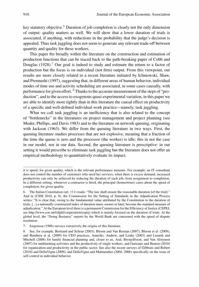
Table 1 describes the unbalanced panel of judges that we study. For the judges whowere already in service on 1 January 2000, we have information also on the cases thatwere assigned to them in the previous year and we can therefore compute a measureof their backlog at the beginning of the period under study. For the judges who tookservice during the period of observation (or less than one year before 1 January 2000)we analyze their productivity starting from one year after they join the court, in orderto give them time to settle in. All the cases assigned to these judges during the first yearof service (including those that were transferred to them from previous judges who leftfor another office or retired) are nevertheless counted to compute their backlog at thebeginning of the second year of service in which we start to analyze their productivity.Thus all the judges that we analyze have at least one year of tenure and for eachone we know the backlog of not-yet-disposed cases at the beginning of the period ofobservation.12

12. If a judge retires or is transferred to a different court (for whatever reasons) his/her cases are eitherall assigned to a new judge (thereby going in the initial backlog of the substitute) or they are distributedrandomly to all the other judges in the court. We will later discuss the implications of these events for theeconometric analysis.


TA

BL

E1.

The

pane

lstr

uctu

re.

Tota

lnum

ber

ofw

eeks

ofse

rvic

e%

wee

ksof

assi

gnm

ent

Ave

rage

num

ber

ofne

wca

ses

per

wee

kSt

anda

rdde

viat

ion

ofne

wca

ses

per

wee

k

Num

ber

ofw

eeks

ofse

rvic

epe

rye

ar

2000

2001

2002

2003

2004

2005

Judg

e(1

)(2

)(3

)(4

)(5

)(6

)(7

)(8

)(9

)(1

0)

152

5252

5252

826

898

8.1

3.6

250

5230

..

.13

297

7.4

3.8

352

5252

5052

5231

099

114.

54

5252

5252

5212

272

989.

64.

55

5252

5046

5031

281

999.

33.

86

5032

5252

4917

252

948.

55

752

5228

1.

.13

395

7.6

4.3

849

5252

44.

.19

798

8.6

4.3

952

5250

5252

5231

098

115.

310

5252

5246

5252

306

9910

4.2

1150

5252

5252

3629

499

94

1252

4952

47.

.20

098

94.

713

5052

5252

5212

270

999.

64

14.

..

1452

5211

896

114.

815

5052

4849

4447

290

989.

64.

416

5252

5252

5252

312

9911

4.6

1752

5052

5252

5030

899

9.4

3.8

1850

5250

5252

5230

899

114

1952

5252

5252

4830

899

115

20.

.8

5152

5216

310

09.

95.

521

..

4049

4852

189

100

9.2

3.9

Tota

l92

191

192

891

786

767

75,

221

989.

74.

5

Not

es:

Col

umns

(1)–

(6)

repo

rt,f

orea

chju

dge,

the

num

ber

ofw

eeks

ofse

rvic

ein

each

year

.Aw

eek

ofse

rvic

eis

aw

eek

inw

hich

the

judg

em

ayre

ceiv

eca

ses.

The

num

ber

ofye

arly

wee

ksof

serv

ice

isno

t52

inth

efo

llow

ing

situ

atio

ns:

whe

nw

est

art

obse

rvin

gth

eju

dge

duri

ngth

eye

ar(l

eavi

ngou

tth

efir

stye

arof

tenu

reth

atw

edo

not

cons

ider

,in

orde

rto

lett

heju

dge

settl

ein

),w

hen

the

judg

ele

aves

the

cour

tdur

ing

the

year

orw

hen

he/s

heha

sa

peri

odof

just

ified

abse

nce

(e.g

.,si

ckne

ss;m

ater

nity

leav

e)of

atle

ast1

wee

k.C

olum

n(7

)re

port

sth

eto

taln

umbe

rof

wee

ksof

serv

ice

for

each

judg

eov

erth

epe

riod

ofob

serv

atio

nw

hile

colu

mn

(8)

show

sth

efr

actio

nof

tota

lwee

ksof

serv

ice

inw

hich

the

judg

ere

ceiv

esat

leas

tone

case

.Bec

ause

ofra

ndom

assi

gnm

enti

nso

me

wee

ksof

serv

ice

judg

esm

ayno

trec

eive

case

s.T

hela

sttw

oco

lum

nsre

port

the

aver

age

wee

kly

wor

kloa

d(n

ewas

sign

edca

ses

per

wee

k)an

dits

stan

dard

devi

atio

n.


Columns (1)–(6) of Table 1 show, for each judge, the weeks of service in eachyear. Weeks of service are those in which the judge must be available to receive newcases. In Italy, as in other countries, the law (Art. 25 of the Constitution) requires thatjudges receive a randomly assigned portfolio of new cases.13 Our econometric strategycrucially relies on this random assignment, which is designed to ensure the absenceof any relationship between the identity of judges and the characteristics of the casesassigned to them, including the identity of lawyers. There is a strict social control onthe enforcement of random assignment in order to keep the heated industrial relationspolitical debate out of the court as much as possible. As a result, judges are not allowedto specialize in particular types of labor controversies and cannot trade trials. Moreover,they are not allowed to render themselves unavailable for assignments, unless they aresick for long periods (more than 1 week). In the rare cases in which these eventsoccur, assignments are typically diverted in a random way to other judges. To reducethe possibility of strategic gaming of the random assignment, cases are assigned alsoduring periods of vacation. As a result of these rules, the yearly weeks of service incolumns (2)–(7) of Table 1 are not 52 only in the following situations: when we startobserving the judge during the year (leaving out the first year of tenure that we do notconsider, in order to let the judge settle in), when the judge leaves the court duringthe year or when he/she has a period of justified absence (e.g., sickness; maternityleave) of at least 1 week.14 Column (7) reports the total number of weeks of servicefor each judge over the period of observation, while column (8) shows the fraction oftotal weeks of service in which the judge receives at least one case. There are in total5,221 judge-weeks of service and in 81 of these some judges do not receive cases.It is evident from the table that these weeks of “no assignment while in service” aredistributed randomly across judges and a formal test cannot reject this hypothesis witha p-value of 0.5375.15

Weeks of no assignment are possible, although rare, because of the way in whichrandom assignment is specifically implemented in the court that we analyze. Everymorning the judges in service are ordered alphabetically starting from a randomlyextracted letter of the alphabet. The cases filed during the day are then assigned inalphabetic sequence to the judges in service. For example, if in a given day the extractedletter is B and five cases are filed, only judges with a name starting from B to F willreceive an assignment on that day (assuming one judge per letter of the alphabet).Therefore, within each week judges may receive slightly different workloads in termsof size. The last two columns of the table report the number of cases assigned toeach judge per week on average and the corresponding standard deviations, which areboth very similar across judges and close to the overall weekly statistics of 9.7 cases

13. Other studies have exploited the random assignment of cases to judges for identification: for exampleAshenfelter, Eisenberg, and Schwab (1995) and Kling (2006).

14. Evidently, the Italian legislator assumes that long sickness and maternity are events that cannot bemanipulated to game the assignment of cases to judges.

15. We test this hypothesis using a linear regression for the probability that a judge receives at least acase in a week as a function of judges’ fixed effects.


TABLE 2. Tests for the random assignment of cases to judges.

Rejections at5%

significance

Fraction ofrejections at

5%significance

Correctedsignificance

Rejections atcorrected

significance

Fraction ofrejections at

correctedsignificance N

(1) (2) (3) (4) (5) (6)

Type controversy 26 0.083 0.0008 5 0.016 312Red code case 12 0.038 0.00016 1 0.0032 312Firing case 18 0.058 0.00038 2 0.0064 312Zip code of

plaintiff’slawyer

26 0.083 0.00096 6 0.019 312

Number ofinvolved parties

22 0.071 0.00081 5 0.016 312

Overall 116 0.062 0.00047 17 0.0091 1,872

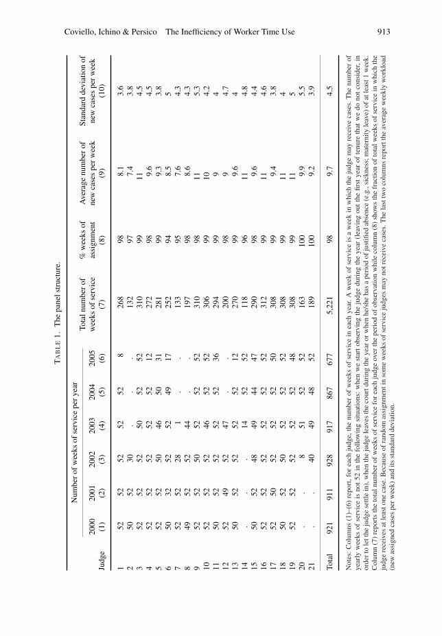
Notes: The table summarizes the evidence on the weekly random assignment of cases to judges, based on Chi-square tests of independence between the identity of judges and five discrete characteristics of cases: type ofcontroversy in 14 categories; a dichotomous aggregation of the types of controversy in red code versus green codecases, by analogy with what happens in a hospital emergency room, where red code cases are those that, accordingto judges, are urgent and/or complicated, thus requiring immediate action and/or greater effort; a dummy forfiring cases; zip code of the plaintiff’s lawyer (55 codes); the “number of involved parties” (capped at 10). Thelast row, Overall, presents joint results for all variables and all weeks. “Rejections at 5% significance” are thenumbers of tests in which p-values are below 0.05. Corrected significance levels are computed with the Benjaminiand Hochberg (1995) multiple testing procedure. Rejections at corrected significance are the numbers of tests inwhich p-values are below the corrected significance levels.

per week with a standard deviation of 4.5. Small sample variability in the number ofcases given to each judge is therefore possible, but this small sample variability is notsystematic and fades away over the long run.

For the same reason, also the characteristics of the assigned portfolios of cases mayoccasionally differ across judges within a week, but in a way that is random and notsystematic. Table 2 reports the summary results of Chi-square tests of independencebetween the identity of judges and six characteristics of cases, conditioning on weeklyassignment: type of controversy in 14 categories; an aggregation of the type ofcontroversy in two categories (“red code” versus “green code” cases)16 by analogywith what happens in a hospital emergency room, where red code cases are thosethat, according to judges, are urgent and/or complicated, thus requiring immediateaction and/or greater effort; a dummy for firing cases; zip code of the plaintiff’s lawyer(55 codes); the number of involved parties (capped at 10). The last row, presents jointresults for all variables and all weeks. The first column reports the numbers of weeks inwhich independence is rejected at the 5% level out of the 312 weeks on which the test isconducted. The corresponding fraction of rejections is in the second column. Since 5%is not the correct significance level in a context of multiple testing, in the third column

16. This dichotomous characterization will be used later in the econometric analysis and therefore it isseparately considered here.


we report the significance levels corrected with the Benjamini and Hochberg (1995)method. When these correct significance levels are used, the number of rejectionsdeclines considerably as shown in the remaining part of the table. Therefore, we canconclude that, within each week, differences in assignments are due only to smallsample variability and are not systematic: in the long run, judges, receive qualitativelyand quantitatively similar portfolios of controversies.

For the purpose of identification of the causal effects of interest these are attractiveand convenient features of our data that compensate for the unfortunate fact that wehave no information of any kind concerning the judges under study, not even age andgender. Differently than in other data sets, which typically have some demographiccharacteristics but do not contain measures of ability and effort, we instead observethe entire history of all the cases assigned to each judge. With this information we canconstruct, as we will see in the next section, very precise time-varying measures oftask juggling, productivity, work scheduling, ability, and effort for each judge.

3. Descriptive Evidence

In this section, we compare judges on the basis of average indicators of task jugglingand performance per week, computed over all the weeks in which each judge isobserved in service.

3.1. Task Juggling

We use the term “task juggling” to characterize any work scheduling practice as aresult of which the tasks of one job are intertwined with the tasks of different jobsassigned to the same worker. Table 3 compares possible measures of task juggling forthe 21 judges considered in this study, treating each trial as a job and hearings as tasks.Table 4 shows the correlations between these measures.

In Table 3, judges are ordered on the basis of their degree of task juggling asmeasured by the indicator reported in the first column. This indicator is the averagenumber of active cases on the desk of a judge, computed over the weeks in which sheis observed. Formally, here and in the rest of this paper, a case is defined as active ata given week if its first hearing has taken place before the end of that week but thecase has not been completed yet by the same date. Of course we do not know the exactmoment in which a judge starts working on cases previously assigned to her, but itseems reasonable to consider the first hearing as a good approximation of this moment.If a judge does not juggle tasks, her number of active cases must be 1. Numbers largerthan 1 indicate that the judge engages in task juggling, because she has scheduledhearings of different cases between the first and the last hearings of other cases. Thetable shows that there is a considerable variability in the degree of task juggling acrossjudges, even if they receive the same workload in terms of quality and quantity becauseof random assignment and full-time working. Judge 11 is working on average on 220


TABLE 3. Measures of task juggling.

Active cases

Active casesat secondhearing

Otherhearings

between firstand secondhearing of a

case

Othernon-firsthearingsbetween

second andthird

hearings of acase

Distance inweeks

between firstand second

hearings of acase

Distance inweeks

betweensecond and

thirdhearings of a

caseJudge (1) (2) (3) (4) (5) (6)

11 220 147 384 269 11 1117 217 143 371 284 13 1615 217 147 405 288 12 1313 213 145 372 279 11 1221 203 137 371 266 13 1310 202 135 358 263 10 1118 197 107 429 252 14 121 192 120 344 252 13 1520 187 125 407 309 11 133 180 116 342 247 8 84 169 112 308 221 8 919 164 109 292 215 8 816 159 102 295 210 8 85 152 110 260 206 7 88 134 86 261 189 7 814 123 58 331 206 13 1312 122 80 232 165 6 67 115 70 239 159 8 89 89 48 195 128 6 72 83 50 185 135 6 76 70 38 163 94 7 7

Notes: The table reports, for each judge, the averages of different weekly measures of task juggling, computedover the weeks of service in which the judge is observed. Active cases are cases that, at the end of a week, haveseen already a first hearing but are not completed yet. Active cases at second hearing are cases that, at the endof a week, have seen already two hearings but are not completed yet. The other measures of task juggling aredescribed by the columns’ headings.

trials in a given week, while judge 6 has only 70 cases contemporaneously open onher desk.

As mentioned in the previous section, judges may want to hold the first hearing of acase as early as possible, to explore the possibility that parties settle, and then delay toa future date the continuation of the trial if settlement does not take place. If this werethe situation, judges would have many cases defined as active with respect to the firsthearing, even if they refrain from task juggling when dealing with subsequent hearings.In other word, they would hold all the hearings of a trial, from the second onwards,without scheduling in the middle of them hearings of other trials, unless they are firsthearings. A judge behaving in this way would have, at every moment in time, only oneactive case defined with respect to the second hearing, even in the presence of more


TA

BL

E4.

Cor

rela

tion

betw

een

alte

rnat

ive

mea

sure

sof

task

jugg

ling.

Act

ive

case

sH

eari

ngA

ctiv

eca

ses

atse

cond

Oth

erhe

arin

gsbe

twee

nfir

stan

dse

cond

hear

ing

ofa

case

Oth

erno

n-fir

sthe

arin

gsbe

twee

nse

cond

and

thir

dhe

arin

gsof

aca

se

Dis

tanc

ein

wee

ksbe

twee

nfir

stan

dse

cond

hear

ings

ofa

case

Dis

tanc

ein

wee

ksbe

twee

nse

cond

and

thir

dhe

arin

gsof

aca

se

Act

ive

case

s1.

00

Act

ive

case

sat

0.98

1.00

seco

ndhe

arin

g(0

.001

)

Oth

erhe

arin

gsbe

twee

n0.

920.

841.

00fir

stan

dse

cond

(0.0

01)

(0.0

01)

hear

ings

ofa

case

Oth

erno

n-fir

sthe

arin

gs0.

960.

930.

961.

00be

twee

nse

cond

and

(0.0

01)

(0.0

01)

(0.0

01)

thir

dhe

arin

gsof

aca

se

Dis

tanc

ein

wee

ks0.

730.

600.

840.

751.

00be

twee

nfir

stan

d(0

.001

)(0

.001

)(0

.001

)(0

.001

)se

cond

hear

ings

ofa

case

Dis

tanc

ein

wee

ks0.

730.

630.

800.

770.

971.

00be

twee

nse

cond

and

(0.0

01)

(0.0

01)

(0.0

01)

(0.0

01)

(0.0

01)

thir

dhe

arin

gsof

aca

se

Not

es:T

heta

ble

repo

rts

the

corr

elat

ions

(and

,in

pare

nthe

ses,

the

p-va

lues

ofth

ete

stth

atth

eyar

eeq

ualt

oze

ro)

betw

een

alte

rnat

ive

mea

sure

sof

task

jugg

ling.

Act

ive

case

sar

eca

ses

that

,att

heen

dof

aw

eek,

have

seen

alre

ady

afir

sthe

arin

gbu

tare

notc

ompl

eted

yet.

Act

ive

case

sat

seco

ndhe

arin

gar

eca

ses

that

,att

heen

dof

aw

eek,

have

seen

alre

ady

two

hear

ings

buta

reno

tcom

plet

edye

t.T

heot

her

mea

sure

sof

task

jugg

ling

are

desc

ribe

dby

the

colu

mn

and

row

head

ings

.


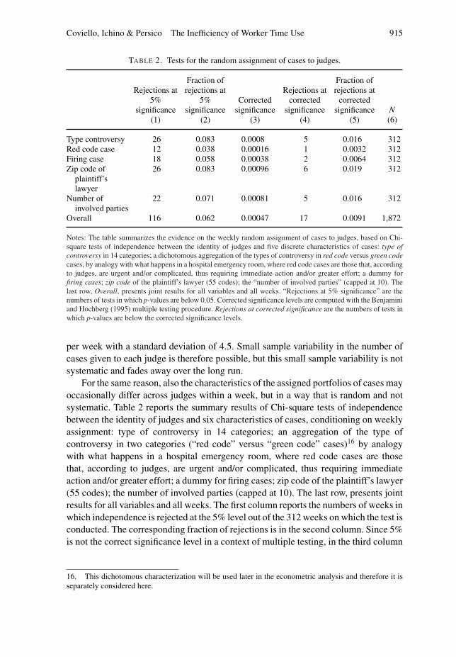
active cases defined with respect to the first hearing. The second column of Table 3reports the number of active cases at the second hearing and it is evident that judgesengage in a considerable amount of task juggling even after the second hearing andindependently of the attempt to induce settlement at the first hearing. Moreover, thecorrelation between the two indicators of active cases is 0.98 (see Table 4), suggestingthat judges who juggle first hearings, juggle also all hearings and vice versa, whilesettlement considerations should affect only the juggling of first hearings.

An alternative way to measure task juggling is to count how many hearings ofdifferent cases are held on average by a judge between the first and the secondhearing of any given case. For a fully non-juggling judge this number should bezero, while column (3) of Table 3 shows that it actually ranges between 163 and429. The correlation between this indicator and the number of active cases is .92 (seeTable 4). A similar indicator can also be constructed for task juggling after the secondhearing, by counting how many non-first hearings are held on average by the judgebetween the second and the third hearing of any given case. This indicator is reportedin the fourth column of Table 3 and ranges between 94 and 309, confirming that taskjuggling extends over the entire life of cases. Also this indicator is highly correlatedwith all the others suggesting that juggling is independent of first hearings.

Finally, similar evidence can be derived from a third way to construct task jugglingindicators, based on the average distance in weeks between subsequent hearings ofcases. The last two columns of Table 3 show that the intervals between first and secondhearings and between second and third hearings range on average between 6 and14–16 weeks and the correlation between the two measures is 0.97. The correlationbetween these distance measures and the other indicators is lower, but still quite high(see Table 4).

To conclude, task juggling can be measured in different ways that are highlycorrelated across judges. More importantly, judges who juggle more first hearingsseem to juggle any hearing, as if juggling were unrelated to the need of schedulingfirst hearings to induce a settlement between parties. The number of active cases is themeasure of task juggling that we prefer to use in the analysis that follows, but, given thehigh correlation with other measures, results do not change qualitatively using theminstead.17

3.2. Total Duration and Active Cases

The height of circles (marked by the judge id number) on the vertical axis of the topleft panel of Figure 1 measures the total duration of cases assigned to each judge.Total duration is defined as the number of weeks from filing up to the week in which asentence is deposited by the judge, or the case is settled, or other less relevant outcomesdetermine the end of the trial (see Section 2). On the horizontal axis judges are orderedfrom the slowest one on the left to the fastest one on the right. The height of the

17. We show it for active cases defined at the second hearing in the Online Appendix, downloadablefrom www.andreaichino.it.


2117

2015141 18131011

5 3 8 4197

166 122

9

21172015141

1813101153

8 4 197

166 1229

010

2030

4050

60

Judges: from slow (left) to fast (right)

Duration (weeks) = circle; New cases = square

21

17

20

15

14

1

18

1310115

3

8

4

19

7

16

6

12

2

9

67

89

10


Throughput

21

17

2015

141

18

1310115

3

8 419

7

16

6

12

2

9

22.

53

3.5

4


Hearings per case

2117

20

15

14

1 18

1310

11

5

3

8

4 19

7

16

6

12

29

5010

015

020

025

0


Active cases

2117

2015

141

18

131011

5

3

8

4

19

7

16

6 12

2

9

200

250

300

350

400


Backlog

211720

15

14

1

1813

1011

5

3

8

4

19

7

16

6

12

2

9

1520

2530

35Judges: from slow (left) to fast (right)

Hearings per week

FIGURE 1. Differences of performance between judges with randomly assigned workload. For eachjudge, the figure displays averages of different performance indicators computed over the weeks ofservice. Duration (weeks) is computed from filing until a sentence, a settlement, or another type ofcase conclusion occurs. New cases assigned on average per week are as in column (8) of Table 1.Active cases are cases that have already seen a first hearing before the end of a given week but are notcompleted yet by that date. Throughput is the number of cases completed by a judge during a givenweek. Backlog is the sum of all the cases historically assigned to a judge but not yet completed bythe end of a given week. Hearings per case is the number of hearings that on average are needed bya judge to close a case. Hearings per week is the number of hearings that a judge holds on averagein a week.

squares in the same panel indicates the workload of new cases per week assigned toeach judge on average. This graphic representation makes transparent the heterogeneityof performance, in terms of duration of trials, observed for these judges despite the factthat they receive a workload which is fairly similar in quantity (because we selectedonly judges who receive a full workload) and quality (because of random assignment).

The bottom left panel in the same figure plots the number of active cases orderingagain the judges from the slowest one on the left to the fastest one on the right.The vertical comparison between the left panels of the figure highlights the high andstatistically significant correlation across judges (0.77; p-value < 0.0001) between theaverage number of active cases and the average duration of trials. It is important tokeep in mind that these differences emerge among judges of the same office, who workin exactly the same conditions, with the same secretarial assistance, and with a similarworkload in terms of quantity and quality.


3.3. Throughput and Backlog

For the reasons explained in the Introduction, we prefer to use duration as opposedto throughput, defined as the number of completed cases per week, as a measure ofproductivity. The total cumulative throughput of these judges can only be equal to theinput they receive, in terms of cases exogenously assigned to them. In principle, twojudges may be deciding the same number of cases in a given quarter, but for one of themthese cases may have been assigned just recently, while for the other they may be veryold cases. What matters, really, is how long it takes to process the input. Nevertheless,in the top central panel of Figure 1 we show that if keeping too many cases openedat the same time slows down the activity of judges, also the number of cases he/shewill be able to close per week is negatively affected on average. The correlation acrossjudges between throughput and the duration of cases is negative although not stronglysignificant (�0.52; p-value D 0.015).

In line with these considerations, it is not surprising to infer, from the bottomcentral panel of Figure 1, that the fastest judges, with fewer active cases, have onaverage a lower backlog, defined as the sum of all the cases historically assigned toa judge up to the end of a given week and that are not completed yet by the samedate. The correlation between the backlog and the number of active cases is high andsignificant (0.91; p-value < 0.0001).

3.4. Complication of Cases, Ability and Effort of Judges

Although suggestive, our hypothesis concerning the role of task juggling on theproductivity of judges must be confronted with other more obvious and potentiallyrelevant determinants of this performance: in particular, ability and effort.

Consider the average number of hearings that a judge needs to close a case.Without random assignment this statistic would depend on both the difficulty ofthe cases assigned to a judge and on her ability to handle them quickly. But givenrandom assignment, the complication of controversies that judges face should be fairlysimilar, up to small random differences determined by the realization of the assignmentprocedure described in Section 2 . Therefore, differences across judges in the averagenumber of hearings to close a case should mostly capture the unobservable skills thatdetermine how a judge can control the trial and the behavior of parties, lawyers, andwitnesses, in order to reach quickly a decision.

This statistic is plotted in the top right panel of Figure 1, where judges are againordered, on the horizontal axis, from the slowest one on the left to the fastest one onthe right. Here we do not appreciate a correlation with duration as strong as the oneobserved for active cases (bottom left panel of the figure). The correlation betweenduration and the number of hearings per case is positive (0.41) but relatively low andless statistically significant (p-value D 0.07). Inasmuch as being able to decide a casewith fewer hearings is a form of ability of a judge, this descriptive evidence does not


1117

15

13

21

10

18

1

20 3

4

19

16

5

8

14

12

7

9

2

6

0.5

11.

52

2.5

33.

5%

of a

ppea

led

case

s

0 5 10 15 20Judges: from heavy jugglers (left) to mild jugglers (right)

FIGURE 2. The trade-off between quantity and quality in the decision of judges with randomlyassigned workload. For each judge, the figure reports the percent fraction of cases for which anappeal has been filed at a higher-level court.

suggest that such characteristics can alone explain the heterogeneity of the averageduration of trials across judges.

A measure of effort is instead offered in our data by the number of hearings held bya judge in a unit of time. The idea is that, by exerting more effort, a judge can schedulemore hearings per week and in this way can, ceteris paribus, improve her performancein terms of throughput and total duration of completed cases. Other dimensions ofeffort, like for example working at night on reading the documentation of cases, arenot directly captured by this measure. However, note that hearings are the tasks thatmake a trial advance towards completion: working at night translates into effectiveeffort only if it generates more hearings per week. Thus, effective effort is what thisindicator is measuring in the bottom right panel of Figure 1. Also in this case we cannotinfer an evident pattern connecting this measure of effort to performance in terms ofduration: the correlation is negative (�0.12) but low and statistically insignificant(p-value D 0.60).

3.5. Is there a “Quantity versus Quality” Trade-off?

It seems important to consider the possibility of a “quantity versus quality” trade-offin the performance of judges. Could it be that judges who juggle more cases are worsejudges in terms of quality of decisions? The evidence presented in Figure 2 suggeststhat the answer is no, as long as the percentage of appealed cases can be consideredas a good measure of the quality of the judges’ decisions. We acknowledge that theappeal rate is at best an imperfect proxy for the quality of judicial decisions, since the


decision to appeal a sentence depends on a variety of factors including especially thetype of trial in question. In our case the homogeneous nature of the trials (all laborlitigations) and furthermore the random assignment of the cases across judges, alleviatethese concerns. In using appeal rates we follow the bulk of the law and economicsliterature which, in the absence of more detailed information, regards appeal rates asa valid proxy for the quality of judicial decisions.18

There is no evidence that the cases assigned to heavy jugglers on the left of thefigure have a lower probability of appeal than the cases assigned to mild jugglers onthe right. If anything, the opposite seems to hold, given that the correlation betweenthe average number of active cases and the percent of appealed cases across judges ispositive (0.19) although statistically insignificant (p-value D 0.40). As for the effect oftask juggling on completion hazards, in Section 6 we will probe further the descriptiveevidence on appeal rates using an econometric model to explore the possibility thattask juggling causally reduces them, thus originating a trade-off between quantity andquality.

To summarize, the descriptive evidence presented in this section suggests that taskjuggling, as opposed to sequential working, may reduce considerably the performanceof judges in terms of total duration of the cases assigned to them, without apparentcosts in terms of quality of decisions. Indicators of experience, ability, and effort are aswell likely to be relevant determinants of performance, but in a possibly less significantway. To go beyond correlations we now move, in the next section, to the descriptionof the theoretical framework that guides our multivariate econometric analysis.

4. A Theoretical Framework to Estimate the Inefficiency Caused by TaskJuggling

In this section we briefly outline a theoretical model based on Coviello, Persico, andIchino (2014) of a judge who juggles tasks. The model delivers comparative staticsfor the duration of each case assigned to the judge as a function of: the effort e putin by the judge (measured in number of hearings per unit of time); the complexity S

of the cases that the judge deals with (measured in number of hearings necessary toadjudicate a case); the number of cases At the judge chooses to simultaneously workon at time t (which is a measure of the judge’s juggling behavior); and, finally, thenumber of cases which are assigned to the judge.

A judge starts his work life with zero cases, and is thenceforth assigned cases at aconstant rate ˛. The judge does not need to start working immediately on every caseassigned to him. Rather, the judge queues up newly assigned cases and draws fromthat queue at rate �: Once a case is drawn from the queue that case is processed inparallel with all other cases previously drawn from the queue and not yet completed.

18. See, for example, Appendix V in CEPEJ (2011) where the appeal rate is cited as an indicator ofquality of judicial decisions for European courts. See also Mitsopoulos and Pelagidis (2010) for an in-depthanalysis which takes the appeal rate as prima facie proxy of the quality of judicial decisions.


This modeling device allows us to model judges who choose to task juggle a lot (high�) and those who choose to work on a few cases at a time (low �). Each case requiresan amount of effort S to complete and the judge chooses a constant effort rate e.The analysis in Coviello, Persico, and Ichino (2014) proves that, in this scenario, thejudge adjudicates cases at a constant rate !: If, moreover, e is small relative to ˛

then Coviello, Persico, and Ichino (2014) prove that ˛ > !, namely that more casesare assigned in each time period than the judge is able to complete. This theoreticalprediction is consistent with our data: the last row in column (9) of Table 1 shows thatin the 5,221 weeks in which we observe our judges ˛ D 9:7, while from the centraltop panel of Figure 1 we find that ! D 8:2; the number of cases assigned and not yetcompleted indeed grows over time. We shall therefore focus the theoretical analysison the case ˛ > !.

Because the assignment and completion rates are constant it is straightforward tocompute a case’s duration. A case which is assigned to the judge at time t finds a massof exactly

˛t � !t

cases previously assigned but not yet completed. Given an output rate of !, these caseswill take the judge exactly

Dt D .˛t � !t/=! D ..˛=!/ � 1/t (1)

units of time to work through. As soon as the time interval of length Dt has elapsedthe mass of cases assigned prior to t will be completed, and in the next instant casesassigned at t will be completed too. Thus the formula for Dt yields the duration of acase assigned at time t:

We now need to substitute out the variable ! in order to express Dt in terms ofvariables that are chosen by the judge (effort and task juggling) in addition to thejudge’s workload. Proposition 1 in Coviello et al. (2014) proves that the completionrate ! is an increasing function of e=S (the more the judge chooses to work, and thefewer hearings it takes to complete a case, the more cases the judge completes per unitof time) and a decreasing function of �, the rate at which the judge adds to the batchof cases that he simultaneously works on. Formally, we have

! D � .e=S I �/ with �1 > 0 > �2:

The partial derivative �2 is negative because a judge who opens more cases diluteshis effort among more cases and therefore ends up being slowed down.

Plugging the function � into equation (1) and taking partial derivatives yields thefollowing predictions. The duration Dt (the time it takes to complete a case after itis assigned) is: increasing in ˛ (the more cases the judge is assigned, the longer eachcase takes to complete on average); increasing in t (judges become overwhelmed overtime—this implication follows from our parameter restriction ˛ > ! ); decreasing ine=S (the harder the judge works, and the fewer hearings are needed to complete a


case, the shorter the duration); and, finally, increasing in the rate � at which the judgechooses to juggle.

In the next section the sign and magnitude of these effects will be estimated usinga duration model. In the duration model the effect of the workload ˛ will be proxiedfor by the total mass of cases assigned to that judge up to time t (which we call Wt andwhich corresponds to ˛t in the theoretical model). In addition, the rate � at which thejudge chooses to multitask will be proxied for by the amount of cases the judge hasactive at time t (corresponding to At D .� � !/ t in the theoretical model). Using At

as a proxy for � makes sense because if � increases then ! decreases (recall that �2

is negative) and so At increases.

5. The Effect of Task Juggling on the Hazard of Case Completion

The theoretical framework described so far shows that if a judge is induced by anexogenous pressure to increase task juggling, her hazard rate of case completion (i.e.,the probability that her cases are completed exactly t weeks after filing given that theyhave survived until then) declines. In this section we present econometric evidencesupporting this prediction.19

5.1. Non-Parametric Hazard Estimates

We frame the empirical analysis using “weeks from filing” as the unit of elapsedtime and, in Figure 3, we begin presenting Kaplan–Meier estimates of the cumulativehazard of completing a case in week t for two group of judges that we characterize as“heavy” and “mild” jugglers in relative terms. The first group comprises those judgeswho keep at least 180 active cases on their desk (see Table 3), while the others are inthe second group. At any week the cumulative hazard is significantly higher for the“mild” jugglers, in line with the prediction of our theoretical model.

5.2. Parametric Hazard Estimates

To probe the robustness of this evidence controlling for relevant covariates, we use aparametric hazard model with time-varying covariates. In our application we are notinterested in the shape of the baseline hazard but only in how the hazard is shifted with

19. In a previous version of this paper, downloadable from www.andreaichino.it, the econometric analysiswas based on the estimation of the conditional expectation function of the duration of cases using aregression analysis aimed at testing whether this conditional expectation was affected by task juggling.In that context, standard linear instrumental variable methods were used to identify and estimate causaleffects, exploiting the exogenous source of variation generated by instruments constructed with the samelogic that will be described here in Section 5.3. The absence of censoring in our data made that econometricapproach possible and meaningful. It is reassuring that the duration analysis presented in this paper and thenonlinear control function approach that here we use to identify causal relationships, thanks to a suggestionof the editor, lead to qualitatively and quantitatively similar conclusions.


0.00

0.25

0.50

0.75

1.00

Cum

ulat

ive

prob

abili

ty o

f clo

sing

a c

ase

0 20 40 60 80 100Elapsed weeks

Mild Jugglers Heavy Jugglers

FIGURE 3. Kaplan–Meier estimate of the cumulative hazard of case completion for “heavy” and“mild”jugglers. The figure shows the cumulative distributions of the probability of closing a casein a given week conditional on survival up to that week (Kaplan–Meier failure function), splittingjudges between relatively Heavy jugglers and Mild jugglers. The first group includes the 10 judgeswho juggle on average at least 180 active cases; the second group includes the remaining 11 judges(see Table 3).

respect to the baseline by different levels of task juggling. For this reason, we followthe partial-likelihood approach proposed by Cox (1972) and specify the hazard thatcase i , assigned to judge j , is completed in week t after filing as

hijt D h0.t/exp�ˇ1Aijt C ˇ2.e=S/ijt C ˇ3Wijt C ˇ4Zijt C ˇ5Tt C ıj

�D h0.t/�.Xijt ; ‰/; (2)

where Xit D .Aijt ; .e=S/ijt ; Wijt ; Zijt ; Tijt ), ‰ D .ˇ1; ˇ2; ˇ3I ˇ4I ˇ5I ıi /, h0.t/ isthe baseline hazard, and �.Xijt ; ‰/ captures the deviations from the baseline hazardin which we are interested, due to the observables Xijt . The Aijt is the number ofactive cases on the desk of judge j at the end of week t of case i (i.e., task juggling).20

The .e=S/ijt is the number of hearings held by judge j in week t of case i dividedby the average number of hearings needed to close the cases for which a hearing washeld in the same week (i.e., effort standardized by the difficulty of cases treated by the

20. A case is active at week t if it has seen a first hearing before the end of week t but it hasnot been completed yet by the same date. Evidence in the Online Appendix (downloadable fromwww.andreaichino.it) shows that results that use active cases at the second hearing as a measure oftask juggling are qualitatively unchanged, which is not surprising given the high correlation with activecases discussed in Section 3.1.


judge).21 The Wijt is the cumulated sum of cases assigned to judge j up to the endof week t of case i (i.e., total workload); Tt is a set of calendar weekly and yearlydummies to control for time effects, including seasonality, in the most flexible way.Zijt is a set of 14 dummies for the type of controversy.22 The ıj are judges’ fixedeffects. It is important to keep in mind, here and in the rest of the econometric analysis,that the inclusion of judge-specific fixed effects in all our specifications should controlfor any time-invariant judge-specific characteristics. Descriptive statistics for thesevariables are displayed in Table 5.

The main focus of our analysis is on the parameter ˇ1 which measures the causaleffect of task juggling on the completion hazard of cases assigned to judge j aftert weeks from filing. Our theoretical framework states without ambiguity that thiscoefficient should be negative, because more task juggling should reduce the hazard ofjob completion. We predict instead a positive sign for ˇ2, because more effort exertionfor given difficulty of the cases to which that effort is applied (or the arrival of easiercases for given effort exerted by the judge) should increase (or at least not decrease) thehazard.23 As for total workload, our model, as do many others, predicts not surprisinglythat ˇ3 should be negative.

In Table 6, we present maximum likelihood estimates of the coefficients of thehazard specified in equation (2). In the first column, the specification does notinclude judge fixed effects while these effects are included in the second column.Independently of fixed effects, the estimated coefficients for the main variables ofinterest are statistically significant at standard significance levels and correspond tothe prediction of our theoretical framework: task juggling has a negative effect oncompletion hazards while standardized effort has the opposite effect. This invariancewith respect to the inclusion of judges’ fixed effects suggests that the two mainvariables of interest are weakly correlated with unobservable time-invariant judgecharacteristics.24

21. To deal with the potential confounding factor generated by the judge’s choice of which hearings tohold and for which cases in the same week, we have also standardized effort using the average numberof hearings needed to close all the cases held by all judges in the same week, and results are qualitativelyunchanged. These results are reported in the Online Appendix (downloadable from www.andreaichino.it).An alternative way to solve the problem is the IV-fixed-effects strategy described in Section 5.3.

22. Because of random assignment of cases to judges, the inclusion or exclusion of these dummiesdoes not affect the main coefficients of interest, as shown in the Online Appendix (downloadable fromwww.andreaichino.it).

23. Note that, by random assignment (see Section 2), within each unit of time all judges receive portfoliosof cases that differ just because of random sampling. Therefore, if S

:j:> S

:k:it must be either because

judge j has randomly received a slightly more complex portfolio than judge k, or because the portfolio iseffectively identical but judge j is “more able” in the sense that she can close the same portfolio of caseswith fewer hearings on average than judge k. However, inasmuch as the ability of the judge is constant overtime, it is captured by the fixed effects ı

j. Looking instead at the same judge across time, despite random

assignment it can happen that S:jt

> S:j�

, with t < � , either because the ability of judge j increases overtime or because the assigned cases become less difficult on average over time.

24. Only the effect of total assigned workload changes between the two columns, becoming negative,as predicted by the model, only when judge fixed effects are included. This is because, since the panel is


TABLE 5. Descriptive statistics.

Mean sd p25 p50 p75 N

Main outcomeTotal duration in weeks (from filing to disposition) 40 34 19 31 51 50,412

RegressorsActive cases 195 73 147 201 250 50,412Standardized effort 8.2 4 5.7 8.1 10 50,412Total workload 2133 904 1406 2052 2886 50,412

InstrumentsRed cases 10 7.3 5 10 15 50,412Normal cases 34 18 26 39 46 50,412

Components of standardized effortEffort 38 17 27 39 50 50,412Number of hearings for cases worked in a week 4.9 1.1 4.2 4.9 5.5 50,412

Additional outcomeAppeal 0.017 0.13 0 0 0 50,412

Notes: Descriptive statistics for the variables used in the econometric analysis, concerning the 50,412 trialsrandomly assigned to 21 full-time judges of the Labor Court of Milan between 1 January 2000 and 31 December2005. Total duration in weeks is computed from filing until a sentence, a settlement, or another type of caseconclusion occurs. Active cases are cases that have already seen a first hearing before the end of a given weekbut are not completed yet by the same date. Standardized effort is the number of hearings held by a judge in agiven week divided by the average number of hearings needed to close the cases for which a hearing was held inthe same week; the numerator and the denominator of this ratio are the variables effort and hearings needed toclose cases described in the bottom panel of the table. Total workload is the cumulated sum of cases assigned toa judge up to the end of a given week. As for the instruments, they are respectively defined as the numbers of redcode and green code cases assigned to a judge in the five weeks that precede and include a given week (or thenumber of cases assigned in the first month of life of a case if the week is one of the first five of the life of thecase). Red code cases are those that, according to a survey of judges and lawyers, are considered as urgent and/orcomplicated, thus requiring immediate action and/or greater effort. Green code cases are instead the remainingstandard and simpler cases. Appeal is a dummy variable taking value 1 if the case is appealed to a higher court.

To get a sense of the economic significance of these results note that the estimatedcoefficients in columns (1), (2) and (5) of Table 6 can be interpreted as the effectof a one-unit change of each variable on the log hazard. Focusing on the fixed-effects estimates in the second column, suppose that a judge increased by 1% herlevel of task juggling. Since the average number of active cases at the end of a weekis 195 (see Table 5), this means adding approximately two more cases to the onesalready open on the judge’s desk. This change of working schedule would imply a 1%decline in the completion hazard (� ˇ1�A D .0:005 � 1:95/ � 100). To compensatefor this hazard decline with more effort, the judge would have to hold approximately0.43 additional hearings per week .� .ˇ1�A/S=ˇ2 D .0:005 � 1:95/ � 4:9=0:112/,which would represent a 1.1% increase of effort starting from the sample average of

unbalanced and random assignment is on a daily basis, judge fixed effects capture judge-specific differencesin workload assignments for judges operating in non-overlapping periods.


TABLE 6. The effect of task juggling on the hazard of closing a case.

Dependent variable h.t jX/ h.t jX/ Activecases

Standardizedeffort

h.t jX/

Estimation method ML ML OLS OLS ML-ControlStage Second Second First First Second

Variables (1) (2) (3) (4) (5)

Active cases �0.005 �0.005 �0.011(0.0001) (0.0001) (0.004)

[0.004]Standardized effort 0.106 0.112 0.202

(0.001) (0.001) (0.057)[0.051]

Workload/10 0.001 �0.007 1.322 0.025 �0.001(0.0001) (0.001) (0.023) (0.001) (0.004)

[0.004]Number of monthly red cases 0.415 0.043

(0.013) (0.0005)Number of monthly normal cases 0.518 0.030

(0.011) (0.0003)

Cragg–Donald Wald F -statistic 425.6Judge fixed effects NO YES YES YES YESCalendar fixed effects YES YES YES YES YESType of case fixed effects YES YES YES YES YESNumber of judges 21 21 21 21 21Number of cases 50,412 50,412 50,412 50,412 50,412Observations 2,032,449 2,032,449 2,032,449 2,032,449 2,032,449

Notes: In columns (1), (2) and (5) the dependent variable is the hazard that a case is closed in week t after filing,conditional on survival up to week t . Active cases are cases that have already seen a first hearing before the endof a given week but are not completed yet by the same date. Standardized effort is the number of hearings held bya judge in a given week divided by the average number of hearings needed to close the cases for which a hearingwas held in the same week. Total workload is the cumulated sum of cases assigned to a judge up to the end of agiven week. Columns (3) and (4) report the first-stage regressions used to construct the third-order polynomialsof residuals on which the control function estimates reported in column (5) are based. The instruments arerespectively defined as the number of red code and green code cases assigned to a judge in the five weeks thatprecede and include a given week (or the number of cases assigned in the first month of life of a case, if theweek is one of the first five of the life of the case). Red code cases are those that, according to a survey of judgesand lawyers, are considered as urgent and/or complicated, thus requiring immediate action and/or greater effort.Green code cases are instead the remaining standard and simpler cases. The Cragg–Donald Wald F -statistic(Joint) denotes the minimum eigenvalue of the joint first-stage F -statistic matrix. Standard errors in parenthesesare clustered at the case level. Standard errors in square brackets are clustered at the judge level and bootstrappedwith 100 repetitions.

38 hearings per week. Thus, the effect of task juggling is sizable in comparison to theeffect of effort, given the observed average behavior of judges in terms of these twovariables: in percentage terms, an increase in task juggling must be compensated by asimilar increase in effort to keep the hazard rate constant.

To translate the effects of task juggling and effort on completion hazards into effectson the duration of cases, some distributional assumptions are needed. As suggested


by Arellano (2008), the Cox proportional hazard model can be written as a linear

regression for the transformation ƒ.Dij / D R Dij

0 u du of the underlying duration Dij

of case i assigned to judge j

lnƒ.Dij / D �Xij ‰ C �ij (3)

if the error term �ij has an extreme value distribution independent of the regressorsXij . More specifically, if the baseline hazard h0.t/ D 1 then ƒ.Dij / D Dij and theregression simplifies to

lnDij D �Xij ‰ C �ij ; (4)

which implies that the estimated coefficients of the Cox proportional model can beinterpreted as the effect of a one-unit change of each regressor on the logarithm ofduration. Under these functional assumptions, using the estimates in the second columnof Table 6, a 1% increase of task juggling, corresponding to about two additional activecases, would raise the average duration of trials by approximately 1%. At the sampleaverage of 280 days, this would be a reduction of about 3 days. A 1% increase of effort(0.38 more hearings per week) would increase standardized effort by almost 0.08 unitsreducing the duration of trials by 0.89%—that is, approximately 2.4 days at the sampleaverage.

As explained in the next section, however, these estimates may not be consistentfor the causal effects in which we are interested.

5.3. Identification of Causal Effects and Control Function Estimates

Like in the case of omitted variable bias in linear regression, Maximum Likelihoodestimation of the hazard (2) does not guarantee that the causal effects in which we areinterested are identified and estimated consistently because of the possibility that judge-specific time-varying unobservables are not independent of variables in Xijt and atthe same time affect the hazard. Such unobservables must necessarily be independentof the workload Wijt which is randomly assigned (see Section 2), but may not beindependent of task juggling Aijt and standardized effort .e=S/ijt . To see why, letMijt denote one such variable, for example, the bad mood or a health shock of judgej in week t of case i , which could affect at the same time task juggling, effort exertionand completion hazards in that week, generating spurious correlations between thesevariables with no causal interpretation. Suppose for one moment that we could observeMijt perfectly. Then the correctly specified hazard would be

Qhijt D h0.t/exp�ˇ1Aijt C ˇ2.e=S/ijt C ˇ3Wijt C ˇ4Zijt C ˇ5Tt C ıj C �Mijt /

D h0.t/�.Xijt ; ‰/exp.�Mijt

�(5)

and the following condition would hold:

E�!ijt � Qhijt / j Xijt ; Mijt

�D 0; (6)


where !ijt D 1 if case i is closed exactly at t by judge j . This condition says thatany shock affecting the actual completion hazard is random and independent of thedeterminants of the correctly specified parametric hazard Qhijt .

Now suppose that we do not observe Mijt , which is the truth in our case, andthat therefore we can only estimate the misspecified hazard (2). Then, using (6) theexpected difference between the true and the misspecified hazard would be

E�!ijt � hijt / j Xijt

� D E� Qhijt � hijt / j Xijt

�

D h0.t/hE

��.Xijt ; ‰/exp.�Mijt / j Xijt

�� .Xijt ; ‰/

i

¤ 0 (7)

and the estimates of the causal parameters in ‰ would be inconsistent.25

To address this problem we follow Palmer (2013) in using the control functionapproach proposed by Heckman and Robb (1985) adapted to the context of durationanalysis. Consider the first-stage twin regressions

Aijt D ˛A0 C ˛A

1 V 1ijt C ˛A

2 V 2ijt C ˛A

3 Wijt C ˛A4 Zijt C ˛A

5 Tt C ıAj C uA

ijt (8)

.e=S/ijt D ˛e0 C ˛e

1V 1ijt C ˛e

2V 2ijt C ˛e

3Wijt C ˛e4Zijt C ˛e

5Tt C ıej C ue

ijt ; (9)

where V 1ijt and V 2

ijt are exogenous determinants of task juggling and standardizedeffort that are independent of Mijt and do not affect the completion hazard directly.The other regressors are the exogenous determinants of the hazard which are includedin Xijt (note in particular, that Wijt and Zijt are exogenous because of the random

assignment of cases to judges). The residuals uAijt and ue

ijt in these two equations canbe correlated and capture the component of Aijt and .e=S/ijt which depend on Mijt .

Conditioning also on these residuals in the hazard (2) solves the endogeneityproblem and delivers consistent estimates of the causal effects of interest. To see why,

25. Note that if Mijt

and Xijt

were independent, the unobservability of Mijt

would be less problematicbecause equation (7) would become

E�!

ijt� h

ijtj X

ijt

� D �E.exp.�M

ijt// � 1

�h

0.t/�.X

ijt; ‰/

and the unobservability of Mijt

would affect only the estimation of the baseline hazard in which we arenot interested and that would simply be scaled by E.exp.�M

ijt//. The condition (7) would be satisfied

on average and the maximum likelihood estimates of the causal parameters of interest in ‰ would beunaffected and consistent, as long as M

ijtand X

ijtare independent. However, in the context of our

application there is no reason to expect that this should be true.


consider the following augmented specification of the hazard:

Nhijt D h0.t/exp�ˇ1Aijt C ˇ2.e=S/ijt C ˇ3Wijt C ˇ4Zijt

C ˇ5Tt C ıj C g� OuA

ijt ; Oueijt

��D h0.t/�.Xijt ; ‰/exp

�g.uA

ijt ; ueijt /

�; (10)

where g.uAijt ; ue

ijt / is a polynomial in the estimated residual. Using this specification,the expected difference between the true and the augmented hazard would be

E�!ijt � Nhijt j Xijt ; uA

ijt ; ueijt

�D E

� Qhijt � Nhijt j Xijt ; uAijt ; ue

ijt

�

D h0.t/�.Xijt ; ‰/

�E

�exp.�Mijt / j Xijt ; uA

ijt ; ueijt

�

� exp.g.uAijt ; ue

ijt //

(11)

which is equal to zero if the control function exp.g.uAijt ; ue

ijt // is equal to the

conditional expectation E�

exp.�Mijt / j Xijt ; uAijt ; ue

ijt

�. If the control function g.�/

is linear and the conditional distribution �Mijt is normal with appropriate mean andvariance, the equality holds exactly. Otherwise, identification relies on the qualityof the polynomial control function in approximating the conditional expectation ofexp.�Mijt /. While this quality can be assessed by showing that results are robust todifferent specifications of the polynomial g.�/, which is the case in our application,26 thecrucial assumption on which this identification strategy stands is that the instrumentsV 1

ijt and V 2ijt are independent of the omitted determinant Mijt of the hazard. To

construct instruments that satisfy this condition we exploit the lottery that assignscases to judges in the way explained as follows.

Consider a case i , assigned to judge j , that has reached week t from filing. Duringthe t weeks of life of this case, the judge has received (randomly) other cases that havelower seniority than case i because they were filed later. If this judge were workingaccording to a purely sequential work schedule (no task juggling) and if her effortexertion were independent of the future workload, the number and characteristics ofthe cases filed after case i should be completely irrelevant for the completion hazardof case i . This is because the judge would work on the lower seniority cases only afterhaving completed, at the usual pace, case i , whose hazard and effective duration wouldtherefore be unaffected.

Suppose instead that the judge juggles task and/or changes effort exertion as afunction of future workload. Under this assumption, the number and characteristics ofthe trials assigned after the filing of case i would be relevant for the completion hazard

26. In Table 6 we present results based on a third-degree polynomial, but we have experimented withpolynomials of different degrees, obtaining similar results.


and the duration of case i . But this feature of future cases would solve the identificationproblem only under the assumption that there is no channel through which they affectthe relevant outcomes different than the effort devoted by the judge to case i and/or theinsertion of these cases in the batch of active trials on which she is working, instead ofconcentrating first on case i only.

It follows from these considerations that the cases assigned to a judge during thelife of an active case could be used to construct arguably valid instruments for Aijt

and .e=S/ijt :

� because they are randomly assigned (see Section 2), and thus provide an exogenoussource of variation;

� if they affect the duration of case i only when the judge opens these cases beforehaving completed case i (i.e., when the judge juggles more tasks by increasing Aijt )and/or changes her standardized effort .e=S/ijt ; this can occur either because thesecases, being for example more demanding, increase the propensity of the judge tohold hearings in each week (which would be a change in eijt ), or because, againbeing more demanding, they require more hearings to be completed (which wouldbe a change in Sijt ).

There is a possibility that the second of these conditions does not hold andthat future workload assignments affect the duration of a current case through otherchannels beyond the measures of task juggling and standardized effort at our disposal,in which case the instruments described previously would violate the exclusionrestrictions. For example, pressed by future cases that are either difficult or moreinteresting, a judge could devote less time to study a current case, or vice versa.However, it is plausible that this condition holds if what the judge can do under thepressure of future cases ultimately translates only into hearings per unit of time (effort)or into a different scheduling of hearings (task juggling) in order for the duration ofcases to be affected.

To see if our conclusions are confirmed also under this alternative identificationstrategy we proceed in the following way. Note that, as anticipated in Sections 2 and 3,trials are not all homogeneous. On the basis of our conversations with judges andlawyers, the portfolio of cases that judges receive can be divided into two distinctcategories that we label as red code and green code, by analogy with what happensin a hospital emergency room. Red code cases are those that, according to judges,are urgent and/or complicated, thus requiring immediate action and/or greater effort.Green code cases are instead the remaining standard and simpler ones. The arrivalof the two types of cases is subject to potentially different stochastic processes: forexample, firing and compensation litigations, which get a red code, are linked to thelocal business cycle, while litigations on government benefits, which fall in the greencode category, are linked to changes in legislation and bureaucratic regulations whosetiming follows different and more erratic rules. Moreover, as in an emergency room,while it would be perfectly reasonable that a newly arrived red code case begins tobe treated before the disposition of a previously arrived green code case, the opposite


would be less reasonable. Hence we may expect that the arrival of both these typesof cases follow different random processes and have different effects on the workschedules adopted by judges.

In an independent survey we therefore asked a set of judges and lawyers to assigna red code or a green code to the different possible types of cases: 22% (11,153) of the50,412 trials considered in this study ended up being classified in the first group. Onthe basis of this classification, we then use as instruments V 1

ijt and V 2ijt , respectively

for Aijt and .e=S/ijt in equations (8) and (9), the numbers of red code and green codecases assigned to a judge in the 5 weeks that precede and include week t .27 Thesecases have been randomly assigned after the filing of case i and should therefore notaffect the completion hazard of case i if judge j does not juggle tasks or change effort.Descriptive statistics for these instruments are reported in Table 5, while the secondand third columns of Table 6 report the estimates of the first-stage regressions (8)and (9) which are strongly significant (the Cragg–Donald Wald F -statistic is equal to425.6).

The control function estimates of the hazard (10), based on these first-stageregressions, are in the last column of Table 6. As in the case of the estimates ofcolumn (2) of the same table, which control for endogeneity just by including judgefixed effects, also these results match the predictions of our theoretical framework:task juggling and workload have a negative effect on completion hazards whilestandardized effort has the opposite effect. The estimated coefficients are statisticallyless significant, as expected, but we can still reject, at standard significance levels, thatthe coefficients of task juggling and standardized effort are equal to zero. Since thecontrol function approach treats the estimated residuals from the first stages as fixed,the usual asymptotic standard errors are likely to be underestimated. For this reasonthe table reports also boot-strapped standard errors (with 100 replications), which arein any case very similar to the usual ones.28

In terms of economic significance the causal effects of task juggling andstandardized effort estimated by these coefficients are slightly larger than the effectsestimated in column (2), but their relative size is comparable. Note that also theestimates of column (5) can be interpreted as the effect of a one-unit change ofeach variable on the log hazard. Based on these estimates and repeating the thoughtexperiment described previously for column (1), suppose that a judge increased by1% her level of task juggling. Since the average number of active cases at the endof a week is 195 (see Table 5), this means adding approximately two more cases tothe ones already open on the judge’s desk. This change of working schedule wouldimply a 2.1% decline in the completion hazard (� ˇ1�A/ D .0:011 � 1:95/ � 100). To

27. In the first five weeks of life case i , the instrument is the number of cases assigned in the first monthafter the filing of case i . This is because if we used the general rule to construct the instruments in the firstfive weeks of case i , we would capture also cases assigned before the filing of case i .

28. In the Online Appendix (downloadable from www.andreaichino.it) we report results that clusterstandard errors at the judge and judge-week level, and conclusions about significance are essentiallyunchanged.


compensate with effort this hazard decline, the judge would have to hold approximately0.52 additional hearings per week .� .ˇ1�A/S=ˇ2 D .0:011 � 1:95/ � 4:9=0:202/,which would represent a 1.4% increase of effort starting from the sample average of38 hearings per week. Thus, given our identification strategy, also in terms of causalestimates the effect of task juggling is sizable in comparison to the effect of effort and,in percentage terms, an increase in task juggling must be compensated by a significantincrease in effort to keep the hazard rate constant.

Under the functional assumptions described at the end of Section 5.2 to translate theeffects on completion hazards into effects on the duration of trials, using the estimates inthe fifth column of Table 6, a 1% increase of task juggling, corresponding to about twoadditional active cases would increase the duration of cases by approximately 2.1%.At the sample average of 280 days, this would be an increase of about six days. A 1%increase of effort (0.38 more hearings per week) would increase standardized effort byalmost 0.08 units reducing the duration of trials by 1.6%—that is, approximately 4.4days at the sample average.

The reason why the IV-fixed-effects estimates of column (5) are larger in absolutesize than the non-instrumented estimates of column (1) is likely to be related to thefact that different judges feel in different ways the pressure of new cases assigned afterthe filing of a given case, while working on it. Using the terminology of experimentaleconometrics, judges have different degrees of compliance with the assignment totreatment. Inasmuch as our estimates capture the causal effect of task juggling for“compliers”—that is, for judges that are more likely to feel the pressure of futurework assignments, then it is not surprising that the absolute size of the estimates incolumn (5) is larger.

To conclude, the empirical evidence presented in Table 6 confirms the theoreticalpredictions concerning the effects of task juggling. Judges who are induced to jugglemore tasks because they feel the pressure of future assignments of cases, require moretime to complete the cases previously assigned to them. The estimated causal effectof task juggling is not only statistically significant but also quantitatively important incomparison to the causal effect of exerting more standardized effort in terms of morehearings per quarters or fewer hearings to close a case.

Before moving to a consideration of the effect of task juggling on the qualityof decisions, we should mention a large management literature, surveyed by Mark,Gudith, and Klocke (2008), suggesting the existence of a disruption cost ofinterruptions, measurable in terms of additional time to reorient back to an interruptedtask after the interruption is handled. In principle, also an effect in the opposite directionwould be possible if it were “boring” for a judge to keep her attention continuouslyfocused on only a few cases for a long time. In this case an increase in the numberof interruptions would be good for performance because switching attention wouldgenerate a benefit from variety. Our data do not allow to separate these effects onefrom the other and both from the mechanical one studied in our theoretical model.However, our estimates described previously suggest that the boredom effect must beweaker and that the other two effects must prevail, so that task juggling has overall adetrimental effect on duration.


6. The Effect of Task Juggling on the Probability that a Case is Appealed

Increasing completion hazards and reducing the duration of trials are goals that couldpotentially come at the cost of a lower quality of decisions. Before concluding thattask juggling has only detrimental effects, it is necessary to gather evidence on thispossibility. For example, in the presence of positive externalities between the activitiesof a judge on different cases, such that she learns from some trials at the advantageof others and vice versa, task juggling could decrease completion hazards while atthe same time allowing for better decisions on average. A similar effect would takeplace if juggling limited to first hearings (i.e., holding them as soon as possible afterfiling instead of waiting for the closure of cases with higher seniority) could facilitatesettlements which were jointly perceived by parties as better outcomes for their cases.

In Section 3 we have anticipated descriptive evidence (see Figure 2) showing thatjudges who juggle more trials tend to have, on average, higher appeal rates for theircases or at least that they do not have lower rates. Unfortunately, appeal rates are notthe ideal measure of the quality of decisions for a variety of reasons, as we alreadymentioned in Section 3.5, but it is the only measure at our disposal and, in this section,we want to see whether the correlation displayed in Figure 2 is robust in controlling forthe relevant confounding factors suggested by our theoretical framework and whetherit may be given a causal interpretation.

Denoting with Pij D 1 the event that case i , assigned to judge j , is appealed, weestimate the probit model

Pr.Pij D 1/ D ˆ�ˇ1

NAij C ˇ2.e=S/ij C ˇ3xWij C ˇ4Zi C ˇ5Tt C ıj

�; (12)

where ˆ.�/ is the normal cumulative distribution. The right-hand side variables areaverages computed over the weeks between filing and disposition of case i . The NAij is

the average number of active cases that are open on the desk of judge j . The .e=S/ij

is the average standardized effort of judge j . The xWij is the average total workloadassigned to judge j . Zi is a set of 14 dummies for the type of controversy. Tt is a setof calendar weekly and yearly dummies for the week in which case i has been filed.ıi are judge fixed effects.

Results are reported in Table 7, which has the same structure of Table 6. Also inthis case the inclusion or exclusion of judge fixed effects (see the first two columns)leaves the estimates essentially unchanged. Task juggling has a positive effect on theprobability of appeal, although marginally significant. Using the fixed-effects estimatesin the second column, an increase of 100 active cases on the desk of a judge (whichis approximately a 50% increase with respect to the observed sample average of195) would increase her rate of appeal by 0.4 percentage points (a marginal effect ofapproximately 25% at the sample average of 1.7%). Effort has instead a negative effectwhich is more precisely estimated. From the viewpoint of the quantity versus qualitytrade-off, these results confirm the evidence of Figure 2 and suggest that, if anything,task juggling reduces the quality of decisions as measured by appeal rates.


TABLE 7. The effect of task juggling on the probability of appeal.

Dependent variable Appeal Appeal Activecases

Standardizedeffort

Appeal

Estimation method ML ML OLS-FE OLS-FE ML-ControlStage Second Second First First Second

Variables (1) (2) (3) (4) (5)

Active cases/100 0.001 0.004 0.015(0.001) (0.002) (0.034)

[0.022]Standardized effort �0.001 �0.001 �0.008

(0.0001) (0.0004) (0.004)[0.003]

Workload/100 0.0002 0.002 0.046 �0.020 0.001(0.0002) (0.0002) (0.014) (0.021) (0.002)

[0.001]Red code cases 0.039 0.120

(0.013) (0.076)Green code cases 0.036 0.350

(0.016) (0.050)

Cragg–Donald Wald F -statistic (Joint) 77.96Average outcome 0.017Judge fixed effects NO YES YES YES YESCalendar fixed effects YES YES YES YES YESType of case fixed effects YES YES YES YES YESNumber of judges 21 21 21 21 21Number of cases 50,412 50,412 50,412 50,412 50,412

Notes: In columns (1), (2) and (5) the dependent variable is a dummy taking value 1 if the case has been appealedto a higher court and the estimates in each row are the Probit marginal effects of the correspondent variable.Active cases/100 is the average, over the duration of each trial, of the cases that have already seen a first hearingbefore the end of each week but are not completed yet by the same date. Standardized effort is the average, overthe duration of each trial, of the number of hearings held by a judge in each week divided by the average numberof hearings needed to close the cases for which a hearing was held in the same week. Workload/100 is the average,over the duration of each trial, of the cumulated sum of cases assigned to a judge up to the end of the same week.Columns (3) and (4) report the first-stage OLS regression estimates used to construct the third-order polynomialsof residuals on which the control function estimates reported in column (5) are based. The instruments arerespectively defined as the average number, over the duration of each trial, of “red code” and “green code” casesassigned to a judge in a given week. Red code cases are those that, according to a survey of judges and lawyers,are considered as urgent and/or complicated, thus requiring immediate action and/or greater effort. Green codecases are instead the remaining standard and simpler cases. The Cragg–Donald Wald F -statistic (Joint) denotesthe minimum eigenvalue of the joint first-stage F -statistic matrix. Standard errors in parentheses are clusteredat the judge level. Standard errors in square brackets are clustered at the judge level and bootstrapped with 100repetitions.

We exploit the control function approach described in Section 5.3 to obtain causalestimates of the effect of task juggling and standardized effort on the probabilityof appeal based on a different identification strategy, to seek confirmation of theconclusions based on fixed effects. Results based on IV fixed effects are shown in theremaining columns of Table 7. The first stages are in columns (3) and (4). Instrumentswere constructed with the same logic described in Section 5.3 adapted to this context.


Specifically they are the average numbers of red and green code cases assigned to judgej during the weeks after the filing of case i and before its disposition. In the absence ofjuggling and if the judge does not change effort when pressed by future assignments,these cases should not affect the development and conclusion of case i , which shouldtake place before judge j begins to look at them. These instruments are stronglysignificant for the measures of task juggling and standardized effort on the right-handside of the Probit model (12). When the Probit model is augmented with third-degreepolynomial control functions constructed on the basis of these instruments (see column(5) of Table 7) the effect of task juggling remains positive but is now very impreciselyestimated, and a zero causal effect cannot be excluded at standard significance levels.Similarly insignificant is the effect of workload, while standardized effort maintains anegative effect which is more precisely estimated.

In the light of these results, it seems possible to conclude that task juggling doesnot improve the quality of decisions, at least inasmuch as a better quality is measuredby a lower rate of appeal experienced by each judge. If anything, more task jugglingseems to increase the rate of appeal. So while task juggling has a clear negative effecton completion hazards and thus increases the duration of trials, the analysis of appealrates does not suggest the existence of more desirable effects on other dimensions.For these reasons, we think it is worth asking whether the observation of task jugglingamong judges is evidence that judges do not use their time efficiently. We turn to thisquestion in the next section.

7. Quantifying the Social Impact of Task Juggling

In this section we attempt to quantify the magnitude of the social gains that can beachieved by reducing task juggling.

Consider the social benefit from decreasing the duration of trials by one day(� 0:4% at the sample average of 280 days), which can be achieved with a taskjuggling reduction given by .�lnD/=ˇ1 � .0:004/=ˇ1 and thus ranging between 0.7and 0.3 of an active case, using respectively the fixed-effects estimates in column (2)or the IV-fixed-effects estimates in column (5) of Table 6. This social benefit is equalto

B DSocial benefit Judge’s private cost

from � fromone day shorter trials decreasing task juggling

(13)

We examine the two components separately.

7.1. Judge’s Private Cost from Decreasing Task Juggling

One might take the perspective that it costs the judge nothing to reorganize her work-scheduling practices. From this perspective the judge’s private costs of decreasingtask juggling should equal zero. This perspective, while legitimate, begs the questionof why judges are task juggling. What could lead a judge to juggle tasks? Perhaps


the pressure of lawyers who lobby for their case to be opened sooner by the judge;or, perhaps, the judge’s desire to comply with administrative rules requiring cases tobe opened relatively quickly. In either case, one might say that acting against theseconsiderations would cause the judge to incur a private cost. How large might this costbe?

We can make progress on this question if we assume that the judge chooses hisamount of task juggling optimally. What would it take to reduce the durations of allthe judge’s cases by one day? According to our estimates in Table 6, this reductioncan be achieved by an increase in effort ranging between 0.23% (in the case of IV-fixed-effects estimates) and 0.41% (in the case of fixed-effects estimates). At themargin, the judge must equate the cost of effort to the wage. Given the judge’s wage,this range of estimated yearly effort increases corresponds to yearly wage increasesranging, respectively, between €274 and €493.29 This is the shadow value to the judgeof reducing the durations of a year’s worth of cases by one day each with additionaleffort. The same reduction in duration can, equivalently, be achieved, at the sampleaverage of 195 active cases, by a 0.17% decrease of task juggling in the case of theIV-fixed-effect estimates (which means reducing by 0.3 units the number of activecases on the judge’s desk) or by a 0.37% decrease of task juggling in the case of thefixed-effect estimates (which means reducing by 0.7 units the number of active caseson the judge’s desk). On account of the judge’s optimal choice of task juggling, theshadow value of one day shorter duration must equal the cost of reducing task jugglingby these amounts—that is, €274 and €493 respectively. These figures represent an(admittedly rough but reasonable) estimate for the second term in equation (13).

7.2. Social Benefit of Decreasing Task Juggling

We now turn to estimating the social benefit from shortening trial durations. We thinkof the trial as resulting from a worker suing the firm. The disagreement concerns thewage level (the firm, being greedy, fails to increase the workers’ wages sufficiently).The model is worked out in the Appendix. The main point of the model is that thematch may be socially valuable and yet the bargaining between worker and firm mayfail. In this case the worker sues and, at the end of the trial, the judge will force the firmto rehire the worker. Ignoring transfers between workers and firms, which are of noconsequence for welfare, the social benefit of a shorter trial is that an efficient match isrecreated sooner rather than later. The magnitude of this benefit can be conceptualizedas follows (on a daily basis):

Q � w � �; (14)

where Q represents the social value created in the match between worker and firm; wis the outside option earned by a worker who is waiting for the litigation to conclude;and � represents the return earned by the firm on the capital freed up by the missing

29. A judge’s yearly gross salary is approximately €120,000 (see http://jobspot.it/stipendio-lordo-magistrato).


worker. In the Appendix we compute these figures based on national account statisticsand find that the social benefit of a decrease by one day of the duration of a single trialequals about €62. Given that a judge receives on average 504 new cases per year, thetotal yearly benefit for society of one fewer litigation day on a year’s worth of trialsis about 62�504 D €31,248. This number represents an estimate for the first term inequation (13).

7.3. Putting Numbers to Equation (13)

According to our back-of-the-envelope calculation the social benefits from decreasingtask juggling in a year by an amount big enough to reduce trials by one day, rangesbetween 31,248 � 274 D €30,974 and 31,248 � 493 D £30,755 per judge. To graspthe size of these figures, they correspond to about 25% of a judge’s annual salary. Thisnumber is large but not implausible despite the approximations needed to computeit. It should also be noted that we are not adding the direct costs of keeping a casegoing; if we did so the costs of litigation would increase even further relative to ourcurrent large estimate. With all the due caveats, the large size of our estimate reflectsthe social value of improving judicial output, which can be achieved either by reducingtask juggling, or by working more hours, or by hiring more judges.

8. Conclusions

We have presented empirical evidence in favor of the theoretical hypothesis thatindividual work scheduling and time use have significant effects on the speed atwhich workers can complete assigned jobs. We test this prediction on a sample ofItalian judges and show that those who are exogenously induced to juggle more trialstake more time to complete similar portfolios of cases. This effect is a by-product oftask juggling. We argue that task juggling is largely practiced by workers in general,and we show that it is practiced by Italian judges in particular.

In order to identify the impact of task juggling on productivity, we proceed intwo ways. First, we remove the main source of endogeneity including judges fixedeffects in our specifications; second, we construct time-varying instruments based onthe sample realization of the lottery that allocates cases to each judge. The effects thatwe measure are not only statistically significant but also quantitatively important: at thesample means, an exogenously induced 1% increase of task juggling would raise theduration of trials by approximately three to six days and would need to be compensatedby a 1.1% to 1.4% increase of effort in order to keep the duration of trials constant.We believe that our results provide the first empirical estimates of the impact of workscheduling on productivity.

We have considered as well the effect of task juggling on the only measure of outputquality at our disposal (percentage of appeals to higher court), finding no adverse effect.For these judges, therefore, we do not detect a trade-off between quantity and quality.Obviously, this conclusion may vary when looking at different types of workers.


Finally, we discuss the extent to which our results signal that judges are inefficientin their choice about how to allocate time between tasks: specifically, whether theyengage in “excessive” task juggling. Our calculations show that, in order for thecurrent scheduling protocol to be an unconstrained private optimum for judges, theeffort cost of opening fewer cases must equal the cost doing more hearings. This seemsparadoxical because opening fewer cases should not represent a direct cost to thejudge. Therefore we conjecture that there is some unmeasured constraint or externalpressure (e.g., lawyers lobbying) which compels judges to juggle tasks. But, even if theexistence of private inefficiency could be debated, we show that the social inefficiencyof longer trials induced by excessive task juggling has strong theoretical justificationsand can be empirically evaluated: if a judge could reduce task juggling enough to cutthe duration of her trials by one day, this would cause a social gain of about €30,000,which corresponds approximately to one-fourth of a judge’s annual income.

We have derived our results for the specific setting of Italian judges and the policyimplications for them are clear: these judges should be helped and induced to work ina more sequential way, reducing the number of active cases contemporaneously openon their desks for given assigned workload.30 But the message of our paper concerningthe effect of task juggling on the speed of job completion and the inefficiency of timeallocation, is more general because it applies to all those situations in which moreoutput is required, but labor or capital cannot be increased at least in the short run.A more sequential work schedule might offer a solution in these cases, because itincreases output per unit of time at the cost of delaying the beginning date of someprojects but not their end date.

We view the analysis in this paper and its companion (Coviello et al. 2014) as afirst step into the empirical and theoretical analysis of how work scheduling affects theindividual production function.

Appendix: The Inefficiency of Delay in a Firing Litigation

Consider a society with 1 unit of Capital and 1 unit of Labor. If jointly used, Capital andLabor form an employment relationship that generates an output Q, which is formallyreceived by the firm if production is undertaken. This amount must be split between awage w and a profit � . If used separately in alternative activities, Labor earns a wagew > 0 and Capital earns a profit �: Efficiency requires joint production if and only ifQ > w C �:

The judge can make sure that when production is efficient, it takes place evenafter a breakdown in bargaining. How the judge splits the surplus Q � w � � is of noconsequence to efficiency, but it matters for incentives. In what follows, we assume

30. We are starting an experiment in three Italian tribunals of different size, in which we will providejudges who are willing to volunteer with an electronic agenda specifically designed to help them in reducingtask juggling and in scheduling the hearings of each trial in a concentrated and sequential way. The evidencefrom this experiment will be a primary focus of our future research agenda.


that in the case of bargaining breakdown—that is, when production is efficient butthe proposed split is not incentive compatible—the judge sets the wage at the outsideoption of the proposing party. This assumption allows us to simplify the proposer’sobjective function, because from the proposer’s perspective there is no differencebetween the event in which bargaining fails and there is no room for efficiency, andthe one in which bargaining fails but the failure is cured by the judge because there isroom for efficient production.

A.1. Firm Makes Offer, Worker’s outside Option is Private Information

We assume that the firm can make a take it or leave it offer to the worker. Therefore,if w were known to the firm, the firm would be able to fully expropriate the worker bysetting a wage w D w: In this case efficiency would prevail because the firm wouldonly produce if Q � w > �; which is the efficient condition.

In our model, however, w is not known to the firm and is considered a randomvariable with cumulative distribution F . If the firm offers a wage w it will be acceptedonly if w > w; an event which has probability F .w/ : In this case the firm makesQ � w in profits. If the wage is rejected then the firm makes profits �; whether or notthe judge steps in. The firm’s expected profits as a function of the wage offer w are,therefore,

F .w/ .Q � w/ C .1 � F .w// �:

The first-order conditions are

f .w/ .Q � w � �/ � F .w/

D f .w/�.Q � w � �/ � .F .w/ =f .w//

�:

The second-order conditions are satisfied if, for example, .F .w/ =f .w// isincreasing, which is a standard assumption in the literature (uniform satisfies it, forexample). In this case the first-order conditions identify a maximum of the expectedprofits. Let w� be the w which solves

�.Q � w � �/ � .F .w/ =f .w//

� D 0;

that is, our equilibrium wage offer. In the case of the uniform distribution f (), forexample, w� D ŒQ � � =2.

So the firm will offer w� and the offer will be rejected whenever w� < w:

However, this may be inefficient. This is the case whenever Q � � > w: So we havean inefficiency whenever

w� < w < Q � �: (A.1)

In the case of the uniform distribution f (), for example, we have an inefficiencywhenever

.Q � �/=2 < w < Q � �: (A.2)


If the uniform distribution is between 0 and 1, this event has probability .Q � �/=2:

The inefficiency in this event is that no joint production takes place due to a greedyfirm which offers a wage lower than the (unknown to the firm) worker’s reservationvalue. We can see this formally. In this case realized social value equals w C � which,in light of the right-hand side of (A.2), is smaller than Q: Accepted offers are alwaysefficient.

The judge can ascertain the true value of w and make sure that the firm and theworker still get together, when bargaining breaks down inefficiently. In this case, thefaster the better.

A.2. Worker Makes Offer; Firm’s Outside Option is Private Information

We assume that the worker can make a take-it-or-leave-it offer to the firm. Therefore,if � were known to the firm, the worker would be able to fully expropriate the firmby setting a wage w D Q � �: In this case efficiency would prevail because theworker would only make the offer if the wage w D Q � � > w; which is the efficientcondition.

In our model, however, � is not known to the worker and is considered a randomvariable with cumulative distribution G. If the worker offers a wage w it will beaccepted only if Q � w > �; an event which has probability G .Q � w/ : In this casethe worker makes a surplus of w in profits, whether or not the judge steps in. If thewage is rejected then the worker makes surplus w: The worker’s expected surplus as afunction of the wage offer w are, therefore,

wG .Q � w/ C .1 � G .Q � w// w:

The first-order conditions are

�wg .Q � w/ C G .Q � w/ C g .Q � w/ w

D g .Q � w/��w C .G .Q � w/ =g .Q � w// C w

�:

The second-order conditions are satisfied if, for example, G .w/ =g .w/ isincreasing, which is a standard assumption in the literature (uniform satisfies it, forexample). In this case the first-order conditions identify a maximum of the expectedprofits. Let w� be the w which solves

��w C .G .Q � w/ =g .Q � w// C w� D 0;

that is, our equilibrium wage offer. In the case of the uniform distribution f (), forexample, w� D ŒQ C w =2.

So the worker will offer w� and the offer will be rejected whenever w� > Q � �:

However, this may be inefficient. This is the case whenever Q � � > w: So we havean inefficiency whenever

w� > Q � � > w;


or equivalently whenQ � w� < � < Q � w:

In the case of the uniform distribution, for example, we have an inefficiency when

.Q � w/=2 < � < Q � w:

The inefficiency in this case is that the worker asks for a high salary, which is sometimestoo high.

The judge can ascertain the true value of � and make sure that the firm and theworker still get together, when bargaining breaks down inefficiently. In this case, thefaster the better.

A.3. The Social Benefit of One Fewer Day of Trial Duration

Whether it is the worker or the firm that makes take-it-or-leave-it offers to the otherside, in case of a litigation, society gains

Qt � w t � � t ; (A.3)

if the judge decides on day t instead of day t C 1, where subscripts indicate thateach variable is measured over the period of one day. This expression has empiricalcounterparts that allow us to approximate its monetary value in the Italian context.

We focus on year 2009, the last one for which all the necessary information isavailable. Using Italian National Accounting Statistics provided by ISTAT 31 the dailyvalue added of a full-time average worker is €171.69, which we take it as a proxy forQt .

Slightly more complicated is to compute W . During a firing litigation a worker canapply for a job at a different firm and take unemployment benefits for at least 1 yearafter firing until she finds a new job. In principle, from the viewpoint of the worker,her outside option could be computed as the weighted mean of the daily averagelabor earning of an Italian employee and of the corresponding daily unemploymentbenefit, using the unemployment rate to construct the weights. But from the viewpointof society, unemployment benefits are a transfer that should have no role to play inefficiency calculations. Therefore, the “productive outside option” of the worker wouldsimply be the average daily wage multiplied by the hazard of finding a job after havingbeen fired. We are not aware of reliable estimates of this hazard, nor do we have suitabledata to generate such an estimate. To be conservative, we assume a competitive labormarket, in which the fired worker can always find immediately a job at the averagewage and therefore the hazard of this event is equal to 1. Using again national statisticsprovided by ISTAT, the average daily wage is €102.53, which is our estimate for W .We emphasize that this is most likely an upper bound of a realistic outside option,

31. See www.istat.it. All the other statistics used in what follows come from either ISTAT or the Bankof Italy.


also because workers involved in firing litigation are probably less productive than theaverage worker. But we prefer to be conservative in our calculation, in the sense ofavoiding overestimating the efficiency gain of a shorter trial.

Moving to the firm, we first measure the stock of physical capital per full-time employee using Bank of Italy estimates: the capital–labor ratio can be set at€222,026.78. The question is, what can the firm do with this capital per worker duringthe litigation? It is important to consider that the Italian labor law states that a firedworker must be rehired by the firm if the judge rules that the firing was unjustified. Therisk of having to rehire the worker often induces firms to leave the capital idle duringthe trial. But to be conservative, we can assume that, while the judge decides, the firmcan earn the riskless interest rate on the capital that would otherwise be combined withthe fired worker. Since the interest rate on one year government bonds was 0.0114during 2009, the daily alternative profit for the firm can be set as … D £6.93.

Putting all these figures together, a conservative estimate of the social benefit ofone fewer day of trial in a firing litigation is (in euro)

Qt � W t � …t D 171:69 � 102:53 � 6:93 D 62:23: (A.4)

Given that a judge receives on average 504 new cases per year (9.7 on average ina week), the total benefit for society of one fewer litigation day on all the trials of theyear is €31,248 (D62�504).32

References

Allen, David (2001). Getting Things Done. Penguin.Arellano, Manuel (2008). Duration Models. Class notes. www.cemfi.es/arellano/duration-

models.pdf.Ameriks, John, Caplin Andrew, and John Leahy (2003). “Wealth Accumulation and the Propensity

To Plan.” Quarterly Journal of Economics, 118, 1007–1047.Aral, Sinan, Erik Brynjolfsson, and Marshall Van Alstyne (2007). “Information, Technology and

Information Worker Productivity.” NBER Working Paper No. 13172.Ashenfelter, Orly, Theodore Eisenberg, and Stewart J. Schwab (1995). “Politics and the Judiciary:

The Influence of Judicial Background on Case Outcomes.” Journal of Legal Studies, 24, 257–281.Bandiera, Oriana, Luigi Guiso, Andrea Prat, and Raffaella Sadun (2008). “What CEOs do.” Working

paper, London School of Economics.Bellotti, Victoria, Brinda Dalal, Nathaniel Good, Peter Flynn, Daniel G. Bobrow, and Nicolas

Ducheneaut (2004). “What a To-Do: Studies of Task Management Towards the Design of aPersonal Task List Manager.” In Proceedings of the SIGCHI Conference on Human Factors inComputing Systems, 24–29 April 2004, Vienna, Austria, pp. 735–742.

Benjamini, Yoav and Yosef Hochberg (1995). “Controlling the False Discovery Rate: A Practical andPowerful Approach to Multiple Testing.” Journal of the Royal Statistical Society B, 57, 289–300.

Bertrand, Marianne and Antoinette Schoar (2003). “Managing with Style: The Effect of Managerson Firm Policies.” Quarterly Journal of Economics, 118, 1169–1208.

32. This calculation rests on the simplifying assumption that the social benefit of one fewer day of firinglitigation approximates the average social benefit of all other trials, for which the calculation would bemore difficult because of less easily obtainable empirical counterparts.


Bloom, Nicholas and John Van Reenen (2007). “Measuring and Explaining Management PracticesAcross Firms and Countries.” Quarterly Journal of Economics, 122, 1351–1408.

Bloom, Nicholas, Carol Propper, Stephan Seiler, and John Van Reenen, (2009). “The Impact ofCompetition on Management Practices in Public Hospitals.” Working paper, London School ofEconomics.

Bohn, Roger (2000). “Stop Fighting Fires.” Harvard Business Review, 78, 83–91.CEPEJ (2011). European Commission for the Efficiency of Justice. https://wcd.coe.int/

ViewDoc.jsp?idD1872077&SiteDCOECobb, W. Charles and Paul H. Douglas (1928). “A Theory of Production.” American Economic

Review, 18(2), 139–165.Covey, Stephen (1989). The Seven Habits of Highly Effective Leaders. Simon and Schuster.Coviello, Decio, Nicola Persico, and Andrea Ichino (2014). “Time Allocation and Task Juggling.”

American Economic Review, 104(2), 609–623.Cox, David R. (1972). “Regression Models and Life-Tables.” Journal of the Royal Statistical Society

B, 34, 187–220.CSM (2010). CONSIGLIO SUPERIORE DELLA MAGISTRATURA, Quarta Commissione.

Gruppo di lavoro per la individuazione degli standard medi di definizione dei procedimenti.Relazione 2010.

DellaVigna, Stefano (2009). “Psychology and Economics: Evidence from the Field.” Journal ofEconomic Literature, 47, 315–372.

DellaVigna, Stefano and Ulrike Malmendier (2004). “Contract Design and Self-Control: Theory andEvidence.” Quarterly Journal of Economics, 119, 353–402.

DellaVigna, Stefano and Ulrike Malmendier (2006). “Paying Not to Go to the Gym.” AmericanEconomic Review, 96(3), 694–719.

Esposito, Gianluca, Sergi Lanau, and Sebastiaan Pompe (2014). “Judicial System Reform in Italy—AKey to Growth.” International Monetary Fund Working Paper, 14/32.

Frantz, Roger (1992). “X-Efficiency and Allocative Efficiency: What Have We Learned?” AmericanEconomic Review: Papers and Proceedings, 82(2), 434–438.

Garicano, Luis and Paul Heaton (2010). “Information Technology, Organization, and Productivityin the Public Sector: Evidence from Police Departments.” Journal of Labor Economics, 28,167–201.

Gibbons, Robert and John Roberts (2010). Handbook of Organizational Economics. PrincetonUniversity Press.

Gonzalez, M. Victor and Gloria Mark (2005). “Managing Currents of Work: Multi-tasking AmongMultiple Collaborations.” In ECSCW 2005: Proceedings of the Ninth European Conference onComputer-Supported Cooperative Work, 18–22 September 2005, Paris, France, edited by H.Gellersen et al., pp. 143–162.

Heckman, J. James and Richard Robb (1985). “Alternative Methods for Evaluating the Impact ofInterventions: an Overview.” Journal of Econometrics, 30, 239–267.

Ichniowski, Casey, Kaathryn Shaw, and Giovanna Prennushi (1997). “The Effects of HumanResource Management Practices on Productivity: A Study of Steel Finishing Lines.” AmericanEconomic Review, 87(3), 291–313.

Jackson, R. James (1963). “Jobshop-like Queueing Systems.” Management Science, 10, 31–142.Jorgenson, W. Dale (1986). “Econometric Methods for Modeling Producer Behavior.” In Handbook

of Econometrics, Vol. III, edited by Zvi Griliches and M. D. Intriligator. Elsevier, pp. 1841–1915.Kling, R. Jeffrey (2006). “Incarceration Length, Employment, and Earnings.” American Economic

Review, 96(3), 863–876.Lusardi, Annamaria and Olivia S. Mitchell (2008). “Planning and Financial Literacy.” American

Economic Review: Papers and Proceedings, 98, 413–417.Mark, Gloria, Daniela Gudith, and Ulrich Klocke (2008). “The Cost of Interrupted Work: More

Speed and Stress.” In Proceedings of the SIGCHI Conference on Human Factors in ComputingSystems, Florence, Italy, April 2008, ACM Press, pp. 107–110.

Mitsopoulos, Michael and Theodore Pelagidis (2010). “Greek Appeals Courts’ Quality Analysis andPerformance.” European Journal of Law and Economics, 30, 17–39.


Palmer, Christopher (2013). “Why Did So Many Subprime Borrowers Default During the Crisis.”Working paper, MIT.

Moder, J. Joseph, Cecil R. Phillips, and Edward Davis (1983). Project Management with CPM, PERTand Project Diagramming. Van Nostrand Reinhold.

Mullainathan, Sendhil and Eldar Shafir (2013). Scarcity: Why Having Too Little Means So Much.Henry Holt.

Perlow, Leslie (1999). “The Time Famine: Toward a Sociology of Work Time.” AdministrativeScience Quarterly, 44, 57–81.

Repenning, Nelson (2001). “Understanding Fire Fighting in New Product Development.” Journal ofProduct Innovation Management, 1, 285–300.

Supporting Information

Additional Supporting Information may be found in the online version of this articleat the publisher’s website:

Online Appendix for “The Inefficiency of Worker Time Use”

the inefficiency of worker time use - hec...

Documents