1

THE INCOME ELASTICITY GAP AND ITS IMPLICATIONS FOR ECONOMIC

GROWTH AND TOURISM DEVELOPMENT: THE BALEARIC VS THE CANARY

ISLANDS

Federico Inchausti-Sintes Universidad de Las Palmas de Gran Canaria

Facultad de Economía, Empresa y Turismo. D.2.15 35017 Las Palmas de Gran Canaria, Spain.

federico.inchausti@ulpgc.es

Augusto Voltes-Dorta University of Edinburgh Business School

Management Science and Business Economics Group EH8 9JS Edinburgh, United Kingdom

avoltes@becarios.ulpgc.es

Pere Suau-Sanchez

Universitat Oberta de Catalunya, School of Business and Economics, Av. Tibidabo, 39-43, 08035 Barcelona, Spain and

Cranfield University, Centre for Air Transport Management, Martell House, University Way, Cranfield, MK43 0TR, UK psuau@uoc.edu

Inchausti-Sintes, F.; Voltes-Dorta, A.; Suau-Sánchez, P. (2020): "The income elasticity gap and its implications for economic growth and tourism development: the Balearic vs the Canary Islands". Current Issues in Tourism [10.1080/13683500.2020.1722618]

ABSTRACT

The Balearic and the Canary Islands are two well-known tourism-led economies. They both

experienced a tourism boom during the same decades, and, hence, they developed a similar

productive-mix. Nevertheless, there are strong economic differences between the two regions. While

the Balearic Islands enjoy a high GDP per capita, the Canary Islands show a more modest

performance. The results of a panel data regression confirm our hypothesis that they differ

substantially in terms of income elasticity of tourism. It is two times higher in the Balearic Islands

than in the Canaries, which indicates the first is perceived as a more luxurious destination.

Furthermore, the results of a dynamic computable general equilibrium model show that the Canaries

would converge in GDP per capita with the Balearic Islands if they attracted tourists with a similar

profile as the latter.

Keywords: Income elasticity; economic growth; tourism-led economies; dynamic computable general equilibrium.

2

1. INTRODUCTION

Before the 1960s, the Canary and the Balearic Islands had different economic patterns. The former

was an agriculture-led economy with a strong export orientation (Millares, Millares, Quintana &

Suárez, 2011). In 1852, the the ‘free port law’ was approved, which sought to promote the

industrialization of the Canary Islands. The law helped to boost both trade and the economy; but the

industrialization never happened (Bergasa & González-Viéitez, 1969). On the contrary, the Balearic

Islands has historicaly shown better economic performance. By 1800, the archipelago already

enjoyed a high literacy rate and a GDP per capita comparable with the richest Spanish regions

(Manera, 2006). The industrial sector represented an important share of the regional economy (24%)

during the XIX century, even though it was mainly focused on low value-added products with low

salaries and technological development (Manera & Parejo, 2012; and Manera, 2006). However, the

advent of tourism during the 1960s and ‘70s led to a strong change in the productive mix of both

archipelagos. Since that time, tourism has been, by far, the real motor of economic growth. For

instance, by 1975, the service sector represented 68.1% of the Balearic economy (Alcaide, 2003).

Indeed, the rise in tourism activity has produced a redistribution of resources from industry to

services (Copeland, 1991). According to Capó, Riera, and Rosselló (2007) and Inchausti-Sintes

(2015), this ‘de-industrialization’ is a consequence of the nature of tourism, which erodes traditional

exporting sectors. The first study distinguishes two key periods that explain this trend: first, the

tourism boom between 1965 and 1974, when the GDP grew 6.4% and 7.3% for the Balearic and the

Canary Islands, respectively, and with capital accumulation explaining more than a half of this

growth. The second key period took place between 1995 and 2000, as the trend reversed and

employment became the main source of economic growth. The consequent reduction in capital

intensity lead to a productivity drop in both archipelagos.

3

Nowadays, both regions are major sun-and-beach destinations in Europe. According to the Spanish

National Statistics Institute (INE), 81 million tourists visited Spain in 2019, 14 million of which

(17%) went to the Canary and Balearic Islands. Both archipelagos have shown similar levels of

human development in the last decades (Herrero, Soler & Villar, 2012). However, the differences in

economic performance still remain (see Figure 1 left). While the Balearics enjoy above-average

levels of GDP per capita, the Canary Islands are 18% below the national average in 2017. The

unemployment rate also differs (Figure 1 middle). The Balearics have an unemployment rate with

strong seasonal variation, yet still around the national average. On the contrary, the Canary Islands

are always above the national average. In terms of productivity, between 2008 and 2014, the tourism

sector and its associated employment in the Balearic Islands represent 42% and 29% of the GDP,

respectively. The same measures for the Canary Islands are 29% and 33% (Exceltur, 2015). Thus,

the Balearics obtain a higher tourism outcome with less labor. A possible reason is that, while the

Canaries experience a higher expenditure per international visitor, stays in the Balearics are, on

average, shorter in duration and this translates into higher average daily expenditure in peak season

(Figure 1, right). Further evidence of the strength of the Balearic tourism sector can be found when

looking at the level of foreign investment. According to the Spanish Institute for Foreign Trade

(ICEX), between 1993 and 2018, companies based in the Balearics accumulate 2.2 billion euro in

global investments in the accommodation sector, which is 8.41 times higher than the ones made by

Canarian firms. The income generated by such investments also contributes to the economic gap

between both tourism-led economies.

[Table 1 about here]

[Figure 1 about here]

4

We hypothesize that a difference in the income elasticity of inbound tourism must exist in order to

explain the broad gap in economic performance between the two regions. This intuition is supported

by past studies that have established a positive correlation between income per capita, income

elasticity and exports (Bahmani-Oskooee & Kara, 2005; Fieler, 2011; Weldemicael, 2014; or Cherif,

Hasanov & Zhu, 2016). In economic terms, a higher income elasticity implies a higher willingness to

pay as income grows, which, in turn, increases the possibilities of higher valued-added gains,

especially in service-based sectors, like tourism, with a traditional lack of productivity

improvements. However, no previous study has carried out a comparative analysis of tourism income

elasticities between different regions within the same country and its consequences in term of GDP

and employment.

In order to fill this gap, we estimate the income elasticities of inbound tourism in both regions and

quantify their economic impact. To that end, we first carry out a panel data regression on a dataset of

international tourist arrivals to the Canary and Balearic Islands, disaggregated by country of origin

and island of destination, between 2012 and 2016. As expected, we find that income elasticity is

significantly higher in the Balearic Islands. Then, a dynamic computable general equilibrium (CGE)

model is used to quantify the economic differences generated by the elasticity gap. The results show

that the Canaries would converge in GDP per capita with the Balearic Islands if assuming the income

elasticity of the latter. This conclusion has direct implications in regards to the development and

promotion of the Canary Islands as a tourism destination in the future.

The remainder of this paper is structured as follows: Section 2 reviews the literature on the

estimation of income elasticities in tourism studies. Section 3 covers the process of data collection,

the panel data regression and CGE methodology. Section 4 presents the results and discusses their

main implications. Section 5 concludes with a summary of the main findings.

5

2.LITERATURE REVIEW

2.1 Income elasticity and economic growth

Sectoral differences in productivity, alongside with an income elasticity gap, have been linked to the

transition of economic activity from low value-added sectors (e.g. agriculture) toward high value-

added, technological ones (Matsuyama, 1992). This economic progress is mainly triggered by the

rise in costs (especially salaries) as a consequence of economic growth. In the long term, the

economies embarked in this transition see how the less productive labour-intensive sectors tend to be

outsourced in cheaper economies, while focusing on more productive capital-intensive ones which

allow firms to sustain higher salaries (Hoffman, 1969; Hausmann, Hwang & Rodrick, 2007 or

Ricardo, 1821). This economic transition also affects the quantity and quality of the goods traded

internationally. According to Fieler (2011), the production technologies are more diverse in goods

with higher income elasticity, which also generate a large dispersion in prices. Thus, richer countries

that are prone to produce and consume these goods, also have an incentive to trade with them. On the

contrary, developing countries focus more on goods whose technology is similar across countries. As

a result, rich countries trade among them with differentiated goods, whereas the trade with

developing countries occurs primarily with homogeneous goods. Thus, wealthy countries tend to

enjoy an export income elasticity greater, and above one, than those of developing countries

(Bahmani-Oskooee & Kara, 2005). The former also show an import income elasticity lower than the

export one. In the long term, exports will grow faster than imports, which benefits the trade balance,

reduces the potential foreign debt imbalances, and strengthens economic growth (Houthakker &

Magee, 1969; Johnson, 1958).

In term of tourism-led economies, both the strong de-industrialization and tertiarization of their

economies limit the development of highly technological sectors, meaning that the economic

6

evolution described above does not occur. Moreover, tourism, as a service-based activity, tends to

show lower productivity compared to other industrial activities (Acelus & Arozena, 1999; Fixler &

Siegel, 1999; or Nordhaus, 2001). Hence, its capacity to sustain higher salaries is seriously limited.

Finally, these economies are usually small islands located far away from their biggest markets, and

with a strong dependence on imports. Hence, the objective of achieving a favorable export-import

income elasticity ratio, as in most developed economies, is more relevant for tourism-led economies.

2.2 Income elasticity in tourism

There is broad consensus in the literature that international tourism is a luxury good (i.e. income

elasticity higher than one). This was the main result of most studies between the 60s and 80s

(reviewed by Crouch, 1992), and more recent publications (with different geographical scopes, data

sources, and methodological approaches) have confirmed this (See e.g. Algieri & Kanellopoulou,

2009; Falk, 2014; Martin & Witt, 1987; Song, Romilly & Liu, 2000; Untong, Ramos, Kaosa-Ard &

Rey-Maquieira, 2015; Vogt & Wittayakorn, 1998). Smeral (2003) notes how income elasticity is

usually higher than price elasticity but, over the last decades, many authors have noted how global

tourism income elasticities show a decreasing trend due to an ongoing saturation process (Gunter &

Smeral, 2016; Morley, 1998) and the impact of recent economic recessions (Peng, Song, Crouch &

Witt, 2015; Smeral, 2017).

We can mention three main trends on how to interpret income elasticities from the perspective of

local authorities in tourism destinations. First, and the most common, is to aid in forecasting visitor

flows. Knowing the income elasticity of the origin markets allows local authorities to prepare and

react to a foreseeable major drop in inbound flows in the event of an economic recession (Dougan,

2007; Lim, Min & McAleer, 2008; Saayman & Saayman, 2015; Smeral, 2009). The second

application relates to destination marketing: the calculation of market-specific income elasticities

7

aids in market segmentation (Álvarez-Díaz, González-Gómez & Otero-Giráldez, 2015; Lin, Liu &

Song, 2015; Fredman & Wikström, 2018). It has been well-established that income elasticities

change across origin countries (Jensen, 1998; Smeral, 2003; Smeral, 2014) as they are sensitive to

income levels and business cycles. Falk & Lin (2018) and Pham, Nghiem & Dwyer (2017) note how

the estimation of income elasticities for each point of origin facilitates the identification of

underserved and non-saturated markets (those more income-elastic) that can be seen as more

attractive. Thirdly, Smeral (2003) employs income elasticities in the context of an investigation

about the differences in the productivity gap between tourism and manufacturing sectors. These

differences can be partly attributed to the luxury nature of the tourism product. To achieve our

research objectives, we adopt the second and third approaches to discuss income elasticities in our

case study.

From a methodological perspective, most academic studies on the estimation of price and/or income

elasticities of tourism demand employ a country-level approach. This means either looking at

inbound markets for a given destination country (e.g. Jensen, 1998; Morley, 1998; Untong et al.,

2015) or outbound markets for a given country (or countries) of origin (e.g. Song, Romilly & Liu,

2000; Smeral & Witt, 2002; Lin et al., 2015). A common conclusion is that the differences in income

elasticities depend on the nationality of the visitor. Still, there seems to be a gap in the literature

when analysing tourism markets below the country level. Certainly, we can find destination-specific

studies (e.g. Liu, 2016 or Fredman & Wikström, 2018) but income elasticities at an intermediate, i.e.

regional/provincial dimension are not common. The value of disaggregating destination markets is in

the possibility of identifying different levels of market positioning for the regional tourism products

offered within the same country, as some destinations can be perceived as more luxurious than others

based on income elasticities. There is also value on disaggregating origin markets as well below the

country level. For example, Bernini & Cracolici (2016) establish significant differences in the

8

income elasticity of international tourism demand between North and South Italy, linked to the

income gap between these regions. Similar conclusions have been found by Alegre & Pou (2004),

Alegre, Mateo & Pou (2009), and Eugenio-Martin & Campos-Soria (2011). This justifies the value

of a disaggregated approach at an origin level as well.

Most studies employ panel data regression methods to estimate demand functions, from which to

derive income elasticities. Besides the regular OLS regression approaches, we find examples of more

sophisticated techniques such as Autoregressive-Distributed-Lag models (ARDL) (see e.g. Álvarez-

Díaz et al., 2015; Lin et al., 2015), Error Correction Models (ECM) (e.g. Smeral, 2009; Algieri &

Kanellopoulou, 2009), Discrete Choice Logit (e.g. Alegre & Pou, 2004) or a Probit regression

(Eugenio-Martin & Campos-Soria, 2011).

Regarding the dependent variable, most studies employ total international arrivals/departures,

number overnight stays, or visitor expenditure (i.e. tourism exports or imports). Income is typically

defined by measures like the Gross Domestic Product (GDP) per capita of the origin country, with a

Purchasing Power Parity (PPP) correction in case of an international sample (Song, Romilly & Liu,

2000; Falk & Lin, 2018). In regard to price, the use of Consumer Price Indexes (CPI) for the

destination is a staple in the literature as a proxy for the visitor’s cost of living. Martin & Witt (1987)

defended that local CPIs should be converted to the visitor’s own currency by means of an exchange

rate adjustment. Álvarez-Díaz et al. (2015) also recommends the use of sector-specific price indexes

(e.g. accommodation or catering services) as a more precise proxy variable. Also common is to

combine origin and destination CPIs to obtain a measure of relative prices, from which a negative

coefficient sign is still expected if the substitution effect prompted by a more expensive destination

dominates the income effect associated to lower CPI at the origin (Crouch, 1992). There is less

consensus about whether to introduce substitute prices in the specification. Papers like Dougan

9

(2007), Algieri & Kanellopoulou (2009), Smeral (2014), Lin et al. (2015), or Pham et al. (2017) only

employ origin and destination prices, with the latter arguing that introducing a synthetic (and

possibly inconsistent) price index for a bundle of potential competitive destination countries will

diminish the accuracy of the inferential analysis. A final aspect to consider is the potential

endogenous relationship between the dependent variables and the price indicator since it cannot be

assumed that tourism supply will be perfectly inelastic to price, particularly in tourism-dependent

economies (Crouch, 1992). Thus, the use of instrumental variables is commonly seen as well, with

lagged prices being a common solution that aim to capture a “price inertia” effect (Dougan, 2007).

Other common variables include demand shocks (e.g.major sport events), visa restrictions, average

air fares (to control for the visitor’s transportation costs), and other air connectivity indicators, such

as non-stop flight frequencies between the points of origin and destination.

Based on the above, our investigation can clearly contribute to the literature on the estimation of

income elasticities on tourism. While we employ established theories and methods, we offer a level

of disaggregation in the analysis at both origin and destination markets that is more detailed than past

contributions.

3. DATA AND METHODOLOGY

3.1. Datasets

The key source of data for this research is the “Tourist Movement on Borders” (FRONTUR) survey

published by the Spanish National Statistics Institute (INE) and the regional statistical offices from

the Balearic and Canary Islands. This survey provides a breakdown of monthly tourism arrivals to

the major islands according to a selection of visitor nationalities. The dataset was compiled between

January 2012 and December 2016 in order to match the availability of income data. Table 2 provides

10

an overview of visitor arrivals in 2016. The Balearic survey provides disaggregated figures for the

following inbound markets: France, Germany, Italy, the Nordic Countries, and the United Kingdom.

The survey for the Canary Islands includes all those countries and also reports the number of visitors

from Belgium, Ireland, and the Netherlands. In both regions, the major nationalities reported in the

FRONTUR survey amount for more than 90% of the total international visitors. Looking at the

destination islands, the Balearic survey combines the visitors to Ibiza and Formentera, due to the

proximity between the two islands and the latter lacking an international point of entry (e.g. airport).

Similarly, only the five Canary Islands with an international airport are reported (Tenerife, Gran

Canaria, Fuerteventura, Lanzarote, and La Palma). Overall, Germany and the United Kingdom are

the major inbound markets in both regions, with a stronger share of Nordic visitors in the Canaries.

[Table 2 about here]

Despite the similarities stated above, these tourist regions differ strongly when looking at how

international visitors are distributed across the year (see Figure 2). The Balearic Islands show an

extreme degree of summer seasonality, typical of coastal regions in the Mediterranean (Rosselló &

Sansó, 2017), while the Canaries, which enjoy a sub-tropical climate, are clearly a year-round

tourism destination with a slightly higher level of activity during the winter season. This will have

implications at the time of capturing seasonality in our regression model.

[Figure 2 about here]

In order to deliver a more precise analysis on income elasticities for different inbound markets, we

disaggregate the FRONTUR monthly visitor statistics according to airport of origin using data on

monthly airline bookings (i.e. Market Information Data Tapes - MIDT) provided by OAG Traffic

Analyser. This source provides information on travel itineraries and country-of-sale for airline

11

bookings purchased in the selected countries (to remove airline tickets purchased by island residents)

and terminating in the international airports from the Balearic and Canary Islands. The proportion of

visitors allocated to each origin-destination airport pair is equal to the proportion of airline tickets

within the total airline traffic at country-island level. This allows us to separate the visitor traffic

assigned to “Nordic Countries” (see Table 2) to Sweden, Norway, Finland, and Denmark. Figure 3

shows the outcome of this disaggregation step for 2016. The airline MIDT dataset reveals that

visitors from mainland Europe originate from many different points (217 different origins in total).

The vast majority of these airports do not have a direct (i.e. non-stop) flight connection to the islands

and, hence, they depend primarily on their national hubs to reach the tourism destinations with at

least one flight connection. These origin markets would remain “hidden” if only employing flight

schedules to/from the island airports in this step.

[Figure 3 about here]

Each origin market is assigned a regional measure of GDP per capita in purchasing power standards

at a NUTS 2 level (based on the location of the respective airport). This information is available with

annual frequency in Eurostat until 2016 (at the date of access). We also gathered NUTS 3 income

data for the destination islands to use it as an instrumental variable.

3.2 Panel data regression

An unbalanced panel dataset of 31,844 observations was obtained. This includes a cross-section of

913 origin-destination airport pairs (217 origin airports from 11 countries travelling to 8 destination

islands) over 12∙5=60 time periods (January 2012 to December 2016). In order to facilitate the

interpretation of the estimation results in terms of demand elasticities, a double-log specification was

employed. Our basic model is shown in Equation 1:

12

(1) 𝑙𝑛#𝑣𝑖𝑠𝑖𝑡𝑜𝑟𝑠!,#* = 𝛽$ + 𝛽%𝑙 𝑛#𝑐𝑝𝑖𝑑𝑒𝑠𝑡𝑎𝑑𝑗!,#* + 𝛽&𝑙 𝑛#𝑛𝑜𝑛𝑠𝑡𝑜𝑝!,#* + ∑ 𝛽! ln#𝑔𝑑𝑝𝑝𝑐!,#* ∙!

𝑟𝑒𝑔𝑖𝑜𝑛! + ∑ 𝛽'𝑖𝑠𝑙𝑎𝑛𝑑'' + ∑ 𝛽(𝑐𝑜𝑢𝑛𝑡𝑟𝑦(( + ∑ 𝛽#!𝑚𝑜𝑛𝑡ℎ) ∙ 𝑟𝑒𝑔𝑖𝑜𝑛! + ∑ 𝛽*𝑦𝑒𝑎𝑟**)! +𝑢!,#

(2) 𝑢!,# = 𝑣! + 𝜀!,#

where i=(1,…,913) denotes an origin-destination airport pair and t=(1,…,60) refers to the time

period. β refers to the vector of coefficients to be estimated and 𝑢! denotes the error term which, in

panel data, is disentangled into an unobservable individual specific effect (𝑣!) and the rest of the

disturbance (𝜀!,#) (see equation 2). The Breusch-Pagan multiplier test (Breusch & Pagan, 1980)

supports the panel-data approach (likelihood ratio=2.2E+05) over a pooled one with 1% significance.

The results of a Hausman test to check the correlation of 𝑣! with the explanatory variables

(Hausman, 1978) allow us to employ a random-effects (RE) regression. A White test (55.55) does

not reject the presence of heteroskedasticity at 1% significance, which implies that the model must

be estimated with robust standard errors.

The dependent variable (visitorsit) is defined as the number of visitors in the i-th origin-destination

airport market in month t. As independent variables, our price indicator cpidestadj measures the

“accommodation and restaurants” consumer price index (CPI) of the destination island. The INE

provides three CPI values: one for all the Balearics, another for Tenerife and La Palma, and a third

one for Gran Canaria, Lanzarote, and Fuerteventura. This CPI is adjusted by the relative change in

exchange rates for those origin countries that do not have euros as currencyi. The effect of events like

the Brexit vote (June 2016) on the value of the British Pound makes this adjustment necessary as one

of the top visitor markets experienced a sudden drop in purchasing power with respect to the Euro. A

second adjustment is made for prices at origin via the purchasing power parity exchange rate at a

13

NUTS 2 level sourced from Eurostat (to capture regional differences at origin). Thus, an increase in

cpidestadj refers to an increase in the relative tourism prices at the destination with respect to the

prices in the origin region and measured in the visitors’ own currency. Since this variable is deemed

to have a strongly endogenous relationship with the visitor numbers, we use the GDP per capita in

the destination island (gdppcdest) and the 12-month lagged price as instruments.

Given the insular nature of the destination regions, we also account for the level of air connectivity.

The number of monthly non-stop airline frequencies between each of the sample countries and each

of the islands (nonstop) is the chosen metric. The data comes from the OAG Traffic Analyser. The

potentially endogenous relationship between air connectivity and international visitors is addressed

by employing the 12-month lag of the total direct and indirect airline connections at a country-island

level, as suggested by Koo, Lim, & Dobruszkes (2017) in order to capture how airline networks

naturally developed over time (conx).

A Sargan-Hansen test confirms the existence of endogeneity with cpidestadj and nonstop at 1%

significance, thus supporting the use of a two-stage least squares method (2SLS) with the

aforementioned instruments.

Income is proxied by the GDP per capita of the NUTS 2 region that contains the origin airport

(gdppc). We add an interaction with regional dummies to test the hypothesis that the tourism

products delivered by the Balearic and Canary Islands have different income elasticities.

The specification is completed with a set of dummy variables for the island and origin countries,

which, among other things, can control for different levels of destination loyalty, possibly motivated

by the existence of large communities of expatriates already settled in the islands. We also control

for the seasonal component of visitor traffic with monthly dummies separated by region, as clearly

14

needed from the analysis of Figure 2. The existence of an overall time trend is captured with the year

dummies.

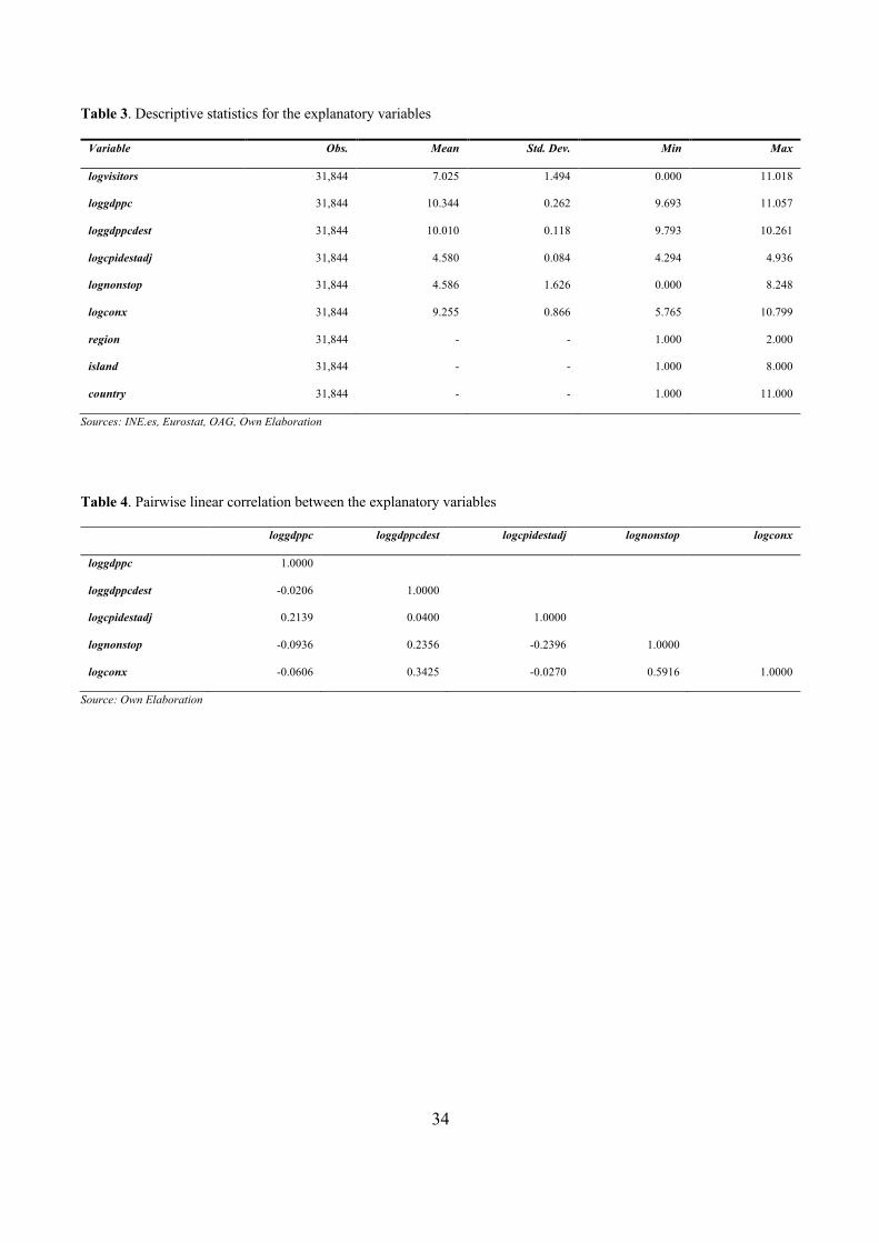
Table 3 provides basic descriptive statistics of the chosen variables. Table 4 shows the pairwise

linear correlation matrix, which allows us to rule out any problems with multicollinearity in the

specification. The largest correlation (59.2%) is present between non-stop and indirect air

connectivity at a country level, which highly desirable for an instrumental variable.

[Table 3 about here]

[Table 4 about here]

The income elasticities estimated in the regression stage are brought forward to the CGE model.

3.3 Dynamic CGE model

The use of CGE models in tourism research is well established, with past contributions focusing on

the effects of tourism on social welfare (e.g. Blake et al., 2006), reducing poverty and inequality (e.g.

Njoya & Seetaram, 2018), or real exchange rates (e.g. Copeland, 1991), with authors commonly

noting its impact on other sectors (e.g. Inchausti-Sintes, 2015). In our case study, we develop a

dynamic CGE model based on the Input-Output Tables (IOTs) of the Canary and Balearic Islands,

sourced from the respective regional statistical offices (ISTAC and IBESTAT). While the last

available tables correspond to 2005 and 2004, respectively, the evolution of sectoral shares in both

regions has not changed dramatically in the last decade. The models were programmed in the

software GAMS using the mathematical programming system for general equilibrium (MPSGE)

(Rutherford, 1999).

15

The regional economies are split into nineteen sectors, with the base model having one government

and one representative household as the main actors. We also assume perfect factor mobility in small

economies, as well as competitive markets and flexible prices. Demand elasticities are sourced from

Hertel (1998).

The central equation in the respective regional CGE models can be written as follows:

(3) 𝐴!,# = 𝛾 @𝜒!𝐷!,#%+!

"#$ + (1 − 𝜒!)𝑀!,#

%+!

"#$H!

"#$%!

,

where M refers to imports and D are domestic goods, both of which can be aggregated in i composite

goods (usually referred to as Armington goods) at time period t (Ai,t). This aggregation follows a

constant elasticity of substitution (CES) function (Equation 3), where , and refer to the

scale parameter, the value share of D, and the elasticity of substitution between D and M,

respectively (Armington, 1969).

Composite goods can be demanded as intermediate goods, and, as such, they enter into a nested

production function (Eqs. 4 and 5) that considers the requirements of capital ( ) and labour ( )

of each economic sector ( ). In the first nest, K and L are transformed with a CES function to

produce a composite good ( ), with , and denoting the scale parameter, the value share of

K, and the sector-specific elasticity of substitution, respectively. In the second nest, the sectoral

production ( ) is determined by combining with the intermediate demand ( )

according to a Leontief function with fixed coefficients α and β.

(4) 𝑎𝑐𝑡𝑣,,# = 𝑚𝑖𝑛 Imin !-&,(,).&,(,)

, /,(,)0(N

gic

dms

,a tK

,a tL

ta

ava h f r

,a tactv

ava

, ,i a tid

16

(5) 𝑣𝑎,,# = 𝜂,#𝜙,𝐾,,#1 + (1 − 𝜙,)𝐿,,#1*!

*being𝜌 = 2+(+%

2+(

The sectoral production is then aggregated by goods: 𝑌!,# = ∑ 𝜓!,,𝑎𝑐𝑡𝑣,,#, , where 𝜓!,, is the value

share of the i-th good in sector a, followed by another CES transformation to disaggregate Yi,t into

domestic ( ) and export goods ( ) as follows:

(6) 𝑌!,# = 𝜀!#𝛿!𝐷!,#(%45) + (1 − 𝛿!)𝑋!,#(%45)*!

,,

where , and denote the scale parameter, the value share of D and the elasticity of

transformation between D and X, respectively.

K and L are demanded by the economic sectors such that 𝐿# = ∑ 𝐿,,#, and 𝐾# = ∑ 𝐾,,#, , where the

sectoral demand of both factors (Ka and La) is defined as follows:

(7) 𝐾,,# = 𝜂,2+(+% [(%+7()8(,)9)\2+( 𝑎𝑐𝑡𝑣,,#

(8) 𝐿,,# = 𝜂,2+(+% [7(8(,):)\2+( 𝑎𝑐𝑡𝑣,,#

Composite goods can also be consumed by households, the government or invested according to

their preferences. In the case of households, the amounts of capital ( ) and labour ( ) available,

as well as the current account deficit ( ) are added up to obtain the overall constraint (Ht) for

consumption and investment decisions (𝐻# = 𝑟#𝐾;,# +𝑤#𝐿_# + 𝑒#𝐶𝐶____). Governments are constrained

(Gt) by the total capital endowment, including both households’ and government’s (𝐾# = 𝐾;,# +

,i tD

,i tX

ie

id T

,H tKtL

tCC

17

𝐾<,#) as well as taxes (𝐺# = 𝑟#𝐾#___ + 𝑡𝑎𝑥𝑒𝑠#), where , and are the salaries, price of capital and

real exchange rate, respectively.

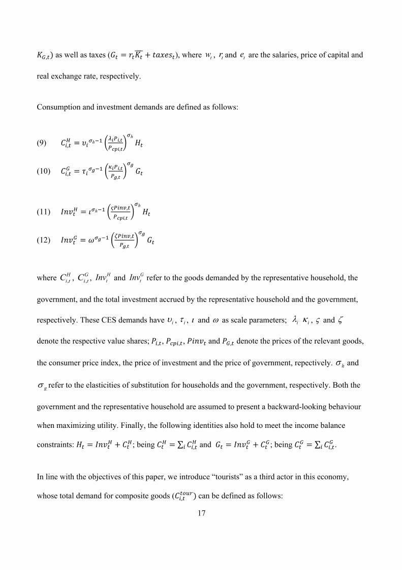
Consumption and investment demands are defined as follows:

(9) 𝐶!,#; = 𝜐!2ℎ+% @=&8&,)8-.&,)H2ℎ 𝐻#

(10) 𝐶!,#< = 𝜏!2/+% @>&8&,)8/,)H2/ 𝐺#

(11) 𝐼𝑛𝑣#; = 𝜄2ℎ+% @?8!@/,#8-.&,)

H2ℎ 𝐻#

(12) 𝐼𝑛𝑣#< = 𝜔2/+% @A8!@/,#8/,)

H2/ 𝐺#

where , , and refer to the goods demanded by the representative household, the

government, and the total investment accrued by the representative household and the government,

respectively. These CES demands have , , and as scale parameters; , and

denote the respective value shares;𝑃!,#, 𝑃BC!,#, 𝑃𝑖𝑛𝑣#and 𝑃<,# denote the prices of the relevant goods,

the consumer price index, the price of investment and the price of government, repectively. and

refer to the elasticities of substitution for households and the government, respectively. Both the

government and the representative household are assumed to present a backward-looking behaviour

when maximizing utility. Finally, the following identities also hold to meet the income balance

constraints: 𝐻# = 𝐼𝑛𝑣#; + 𝐶#;; being 𝐶#; = ∑ 𝐶!,#;! and 𝐺# = 𝐼𝑛𝑣#< + 𝐶#<; being 𝐶#< = ∑ 𝐶!,#<! .

In line with the objectives of this paper, we introduce “tourists” as a third actor in this economy,

whose total demand for composite goods (𝐶!,##DE9)can be defined as follows:

tw

tr

te

,

H

i tC

,

G

i tC

H

tInv

G

tInv

iu

it i w

il

ik V z

hs

gs

18

(13) 𝐶!,##DE9 = 𝜛!2)012+% [F&8&,)

G)\2)012 𝑡𝑜𝑢𝑟𝑖𝑠𝑚#

They are constrained by their expenditure level ( ). denotes the scale parameter; 𝜃! refers

to the value shares of each good, represents the real exchange rate and σtour is the elasticity of

substitution.

The tourism income elasticity estimated in the regression stage is introduced in the CGE model by

adding an extra level of consumption of the relevant goods in the tourism consumption bundle and

simultaneously including this extra consumption as a positive endowment in the tourism income

balance constraint (Stone-Geary consumption demand).

Model closure is ensured with several additional assumptions (Hosoe, Gazawa & Hashimoto, 2010),

such as investment being driven by savings, zero government deficit, fixed global prices and foreign

savings. We also account for unemployment by means of a minimum wage constraint: 𝑤# = 𝑃BC!,#, which implies that unemployed individuals will only work if salaries (𝑤#) compensate the

opportunity cost represented by the consumer price index (𝑃BC!,#). Both models were calibrated

assuming an unemployment rate of 29% and 11.67%, for the Canary and Balearic Islands,

respectively (according to ISTAC and IBESTAT figures).

The dynamic nature of our model also requires us to define annual rates of economic growth (g),

depreciation of capital ( ), and an interest rate ( ). Economic growth is assumed at 1.6% according

to IMF (2019) and the annual depreciation rate is 5% (Escribá-Pérez, Murgui-García & Ruiz-

Tamarit, 2017). Therefore, the initial stock of capital (K0) and the interest rate are determined as

follows: K0 = Inv/(g+δ) and ir =(VK/K0)−δ. Where Inv denotes total investment and VK refers to

the total gross operating surplus.

ttourism

iv

e

d ir

19

The government and the household’s capital endowment change over time as follows:

(15)

(16) ,

where and denote the gross operating surpluses accrued by the household and the

government, respectively. And, and , denote the initial endowment of investment for

the household and the government, respectively.

Finally, we assume an annual increase of 2% in arrivals (this is the shock to be modelled), which is

the forecast established by the World Tourism Organization for Southern Europe in the following 30

years (2010-2030) (UNWTO, 2011). Therefore, we use a time horizon of 21 years in the dynamic

model (2019-2030).

4. RESULTS AND DISCUSSION

4.1 Panel-data regression

Table 5 shows the estimation results for the 2SLS regression. The coefficients of loggdppc.Balearic

and loggdppc.Canaries clearly support our working hypothesis: the Balearic Islands show a tourism

income elasticity of 2.33 which is two times higher than the respective elasticity in the Canary

Islands (1.16). This indicates the first is perceived as a more luxurious destination. According to

Peng et al (2015), the average tourism income elasticity in Europe is 2.4. The Balearic income

elasticity is around the same magnitude than the one estimated for winter tourism in Switzerland

(Falk, 2014) or Japanese tourists in New Zealand (Lim et al, 2008). On the other hand, the income

,, , 1 , 1(1 ) ( )H tH t H t H t tK K VK inv inv ird d

- -= - + + +

, 0, , 1 , 1(1 ) ( )G tG t G t G t tK K VK inv inv ird d=- -

= - + + +

,H tVK

,G tVK

, 0H tinv = , 0G tinv =

20

elasticity in the Canary Islands is closer in value to the Chinese tourist demand to Thailand (Untong

et al, 2015). Still, both values are more optimistic than the global elasticities reported by Gunter and

Smeral (2016) for the period 2004-2013, with a tourism income elasticity well below one (0.2) for

Southern Europe.

We find inbound tourism demand to be price-inelastic: a 1% increase in relative prices decreases

demand by 0.6%. This result is opposite to Crouch (1995), Garín-Muñoz (2006) and Garín-Muñoz &

Montero-Martín (2007), who all argue that sun-and-beach destinations tend to be price-elastic.

According to Peng et al. (2015), the price is also elastic for tourism in Europe (-1.20). On the other

hand, Gunter and Smeral (2016) obtained an inelastic price sensitivity, with some few exceptions, for

the period 1977-2013. For instance, price elasticity is -0.61 at world level, whereas is -0.50 for

Southern Europe.

[Table 5 about here]

[Table 5 (continue) about here]

We can also disaggregate the income elasticities according to geographical market. The estimates are

shown in Table 6, and, as expected, all the Canary Islands show an income elasticity lower than the

Balearic Islands in all cases. The regional-level differences in income elasticity remain statistically

significant at 5% level. There are also differences in the central estimates of income elasticity across

the major origin countries within each region. Thus, our results point to a similar conclusion than that

of Jensen, (1998), Smeral (2003) or Smeral (2014) about the existence of different segments for

inbound tourism demand according to nationality and, hence, to the different preferences and income

levels of these visitors.

21

[Table 6 about here]

In accordance with the established interpretation of income elasticities in relation to product

positioning and market segmentation, it is possible to investigate whether the differences between the

Canary and Balearic Islands can be traced to their current market mixes. The slope graphs provided

in Figures 4 to 6 show the differences in the relative ranking of origin markets according to income

elasticity and share of visitors. Countries with a higher ranking in terms of income elasticity will

perceive the destination as more luxurious and hence, they can be considered as very attractive, non-

saturated, high-yield markets. This ranking can be compared to the actual country market shares in

each island to evaluate whether the islands are currently serving their most attractive inbound

markets. Results show that the minor Balearic Islands of Menorca, Ibiza, and Formentera have the

most distinctive visitor profiles, because their top market (Germany) is also among their most

income-elastic. This suggests a better market positioning as a luxury destination, which is seen very

clearly in the respective branding strategies developed by the local tourism boards (e.g.

www.ibizaluxurydestination.com) that reinforce aspects such as exclusivity that are highly appealing

to these visitors. The other islands, including Mallorca and all the Canaries show a different, more

traditional profile, with income elasticities and market shares showing an inverse rank correlation,

which signals a specialization on massive tourism markets with a higher degree of saturation. Thus, a

second conclusion is that the Balearics achieve better tourism outcomes because they have been able

to offer visitors a more diversified choice of destinations, with minor islands focusing on a luxury

experience while the main island retains its high-end massive appeal. In spite of that, most islands

have room for improvement by growing their most income-elastic market segments. Indeed, the

German and UK visitors to the Canary Islands show evident signs of being a mature market, while

the Netherlands, Belgium, and the Nordic Countries appear to be the best targets for further

development.

22

[Figure 4 about here]

[Figure 5 about here]

[Figure 6 about here]

4.2 CGE model

The economic consequences of the elasticity gap are quantified with a dynamic CGE model, in

which we simulate the Canaries experiencing the same tourism income elasticity than the Balearics

between 2019 and 2030. Two scenarios are presented: in Scenario A, the income elasticity affects

key tourism-related goods (“accommodation”, “catering services”, “real estate”, “rent a car”, “travel

agencies” and “entertainment”). In Scenario B, the income elasticity affects all goods. Both scenarios

are shocked by a 2% annual increase in tourism arrivals. For comparability, we simulated the same

scenarios but for the opposite case: the Balearics having the same elasticity than the Canaries

(Scenarios A* and B*).

According to Table 7, the Canaries would grow between 20% and 40% over the period in Scenarios

A and B, respectively. In total, there would be 82,596 new jobs (3,933 new annual jobs) which

would imply a reduction in the unemployment rate from 20% to 12.75% by 2030 in Scenario A. This

value is similar to the current unemployment rate in the Balearic Islands (11.67%). The estimate of

new jobs created is slightly worse in Scenario B, which can be explained by the higher prices (due to

higher GDP) that reduces the willingness to work. With their own income elasticity, the Baleric

Islands are predicted to grow between 22% and 29%, without a significant reduction in

unemploymentii.

23

[Table 7 about here]

These results can be better contextualized when translating the multiplicative GDP effects into real

values. Table 8 shows the ranking of the Spanish Autonomous Communities by GDP per capita in

2018. The Balearic Islands enjoy a GDP per capita slightly above the national average. On the

contrary, the Canary Islands are located in the lower half with a GDP per capita that is 1.22 and 1.27

times lower than the national average and the Balearic Islands, respectively. However, the

differences in GDP per capita between both archipelagos would reduce from the actual 27% to 4% in

Scenario A, and to -9% in Scenario B as the Canaries would converge in GDP per capita with the

wealthiest Spanish regions. In the opposite situation (Scenarios A* and B*), the Balearics would fall

to the lower half, closer to the Canaries’ current satiation. Thus, it is clear that, ceteris paribus, the

tourism income elasticity plays a key role in the economic performance of both insular regions. This

illustrates the benefits of transitioning towards a higher-end “luxury” destination to tap the more

income-elastic traveller segments.

[Table 8 about here]

4.3 Policy implications

Policymakers and the overall tourism sector in the Canaries should wonder about whether there is a

lack of market identification and/or service quality that prevent high-income tourists from travelling

to their destinations. At first sight, increasing the ability of tourism destinations to achieve better

outcomes clashes with the lower potential for productivity gains traditionally associated to service

activities. However, improvements can still be achieved by means of enhancing quality, which

should be a strategic cornerstone in tourism-led economies. First, local authorities can promote the

investment in better tourism infrastructure as well as in the preservation of the islands’ natural

24

resources. In relation to this, during the last decades, both regional governments have been approving

tourism moratoria laws to restrict the development of tourism accommodation supply while granting

exceptions to hotels upgrading their facilities (Hernández-Martín, Álvarez-Albelo & Padrón-Fumero,

2015).

Secondly, a detailed market analysis and segmentation based on income elasticities seems a suitable

way to identify attractive market segments and guide strategic decisions about where to invest in

destination marketing campaigns and what to advertise. In line with the more diversified choice

presented by the Balearics, these can include promotional actions at the main origin airports of the

target countries that attempt to re-brand some of the minor islands (such as Lanzarote or La Palma)

as places suitable for luxury visitors, while the major islands (Gran Canaria and Tenerife) can

continue their transition towards the high-end massive tourism market. Focusing the development of

the luxury market in the minor islands has the advantage of reduced investments and better chances

of developing a differentiated brand image with respect to the massive tourism offer in the major

islands.

5. SUMMARY

Despite the many similarities between the Balearic and the Canary Islands, a strong economic gap

exists between the two regions. We hypothesize that this gap is linked to a different market

positioning, and thus income elasticities, of the respective tourism products. In order to prove this

intuition, we carried out a panel data regression on international tourism arrivals to the Balearic and

Canary Islands between 2012 and 2016 and we estimate the economic consequences of the elasticity

gap with a CGE model.

25

The results of a panel data regression confirm our hypothesis that income elasticities differ

significantly between both regions. It is two times higher in the Balearic Islands than in the Canary

Islands, which indicates the first is perceived as a more luxurious destination. Overall, the Balearics

offer a more diversified choice of destinations, with minor islands focusing on a luxury experience

while the main island retains its high-end massive appeal. The conclusions of the GCE modelling

indicate that, if the Canaries experienced the tourism income elasticity of the Balearics, the region

will increase its GDP per capita in 22%, thus eliminating the income gap between the insular regions.

These results emphasize the importance of focusing on higher value-added tourist activities. In

tourist terms, this means investing in quality and service innovation by e.g. upgrading tourism

infrastructure while preserving the islands’ natural attributes. Such improvements can be more

effective if they are targeted to the markets with a higher perception of the tourism product on offer,

which can be identified by means of a detailed market segmentation. In the Canaries, marketing

efforts could consider re-branding some of the minor islands as luxury destinations, while the major

islands continue their transition towards high-end massive markets.

Our conclusions, however, should be interpreted with caution, as there are some limitations to our

empirical estimates. First, the sample period (2012-2016) is relatively short and inevitably impacted

by extraordinary events like the global recession, which can compromise the generalizability of our

policy implications to other periods. Unfortunately, the time-series dimension of the dataset is

defined by the availability of MIDT data that is necessary to disaggregate passenger arrivals

according to origin markets. Still, expanding the sample period further back would not have

mitigated the problem since the recession started in 2008, and the beginning of the Arab Spring in

the early 2010s can also be expected to affect the number of passenger arrivals to both regions. A

more recent time series would have allowed us to better capture the impact of the Brexit vote on UK

inbound demand, which is one of the islands’ key markets. Secondly, it is not possible to obtain

26

monthly income data for the travellers, which does not allow us to fully disaggregate the income

elasticity between peak and off-peak periods in the Balearics. This would have been of interest as

travellers’ profiles can be different across the year. Third, there is also a shortcoming in the lack of

socioeconomic indicators in the analysis (e.g. age, group size), that could also serve to illustrate the

differences between the tourism markets served by both regions. All these limitations can be

overcome as data becomes available. Further research can also investigate how and whether the

emergence of low-cost carriers in the Spanish island airports has affected the income elasticities of

inbound tourism over time, by making travel more affordable and perhaps increasing the proportion

of lower-income visitors. In view of the results of this paper, confirming that hypothesis would have

implications on the dilemma faced by local authorities between investing in service quality to attract

more high-end visitors and granting subsidies to low-cost operators to boost inbound traffic. Other

interesting areas to cover relate to how the Balearics seem to benefit from extreme seasonality,

despite the challenges traditionally associated to that characteristic of inbound traffic in the areas of

planning and management of tourism resources.

27

REFERENCES

Acelus F.J. and Arozena, P. 1999. “Measuring sectoral productivity across time and across countries”. European Journal

of Operational Research 1119 (2): 254-266.

Alcaide, J., 2003. “Evolución económica de las regiones y provincias españolas en el siglo XX”. Bilbao: Fundación BBVA.

Alegre, J., and Pou, L., 2004. “Micro-economic determinants of the probability of tourism consumption”. Tourism

Economics 10(2): 125-144.

Alegre, J., Mateo, S., and Pou, L., 2009. “Participation in tourism consumption and the intensity of participation: An

analysis of their socio-demographic and economic determinants”. Tourism Economics 15(3): 531-546.

Algieri, B., and Kanellopoulou, S., 2009. “Determinants of Demand for Exports of Tourism: An Unobserved Component

Model”. Tourism and Hospitality Research 9(1): 9-19.

Álvarez-Díaz, M., González-Gómez, M., and Otero-Giráldez, M.S., 2015. “Research note: Estimating price and income

demand elasticities for Spain separately by the major source markets”. Tourism Economics 21(5): 1103-1110.

Armington, P., S., 1969. “A theory of demand for products distinguished by place of production”. International Monetary

Fund (Staff Papers), 16(1): 159-178. Washington DC, US.

Bahmani-Oskooee, M., and Kara, O., 2005. “Income and price elasticities of trade: some new estimates”. The International

Trade Journal 19 (2): 165-178.

Bergasa. O., and González-Viéitez. A., 1969. “Desarrollo y subdesarrollo de la economía canaria”. 1ª ed. Madrid:

Guadiana.

Bernini, C., and Cracolici, M.F., 2016. “Is participation in the tourism market an opportunity for everyone? Some evidence

from Italy”. Tourism Economics 22(1): 57-79.

Blake, A., Durbarry, R., Eugenio-Martin, J. L., Gooroochurn, N., Hay, B., Lennon, J., & Yeoman, I., 2006. “Integrating

forecasting and CGE models: The case of tourism in Scotland”. Tourism Management, 27(2): 292-305.

Breusch, T. S., and Pagan, A. R., 1980. “The Lagrange multiplier test and its applications to model specification in

econometrics”. The Review of Economic Studies, 47(1): 239-253.

Cherif, R., Hasanov, F., and Zhu. M., 2016. “Breaking the oil spell: the gulf falcons´path to diversification”. Washington

DC: International Monetary Fund.

Copeland, B. R., 1991. “Tourism, welfare and de-industrialization in a small open economy”. Economica, 515-529.

Crouch, G.I., 1992. “Effect of income and price on international tourism”. Annals of Tourism Research 19(4): 643-664.

28

Dougan, J.W., 2007. “Analysis of Japanese tourist demand to Guam”. Asia Pacific Journal of Tourism Research 12(2: 79-

88.

Eugenio-Martin, J.L., and Campos-Soria, J.A., 2011. “Income and the substitution pattern between domestic and

international tourism demand”. Applied Economics 43(20): 2519-2531.

Escribá-Pérez, J., Murgui-García, M.J., & Ruiz-Tamarit, J.R., 2017. “Medición económica del capital y depreciación

endógena: una aplicación a la economía española y sus regions”. Investigaciones regionales- Journal of Regional

Research, 38: 153-180.

Exceltur., 2015. “Estudios del impacto económico del turismo sobre la economía y el empleo de las Illes Balears”.

Available at: https://www.exceltur.org/impactur/#

Falk, M., 2014. “The sensitivity of winter tourism to exchange rate changes: Evidence for the Swiss Alps”. Tourism and

Hospitality Research 13(2): 101-112.

Falk, M., and Lin, X., 2018. “Income elasticity of overnight stays over seven decades”. Tourism Economics 24(8): 1015-

1028.

Fieler, A. C., 2011. “Nonhomotheticity and bilateral trade: Evidence and a quantitative explanation”. Econometrica 79 (4):

1069-1101.

Fixler D. J., and Siegel, D., 1999. “Outsourcing and productivity growth in services”. Structural Change and Economic

Dynamics 10 (2): 177-194.

Fredman, P., and Wikström, D., 2018. “Income elasticity of demand for tourism at Fulufjället National Park”. Tourism

Economics 24(1): 51-63.

Garin-Muñoz, T., 2006. “Inbound international tourism to Canary Islands: A dynamic panel data model”. Tourism

Management, 27(2): 281-291.

Garin-Munoz, T., and Montero-Martín, L. F., 2007. “Tourism in the Balearic Islands: A dynamic model for international

demand using panel data”. Tourism Management, 28(5): 1224-1235.

González A., and Matés, J. M., 2007. “Historia económica de Esapaña”. Barcelona: Ariel.

Gunter, U., and Smeral, E., 2016. “The decline of tourism income elasticities in a global context”. Tourism Economics

22(3): 466-483.

Hausman, J., 1978. “Specification tests in econometrics”. Econometrica 46: 1251-1271.

Hausmann, R., Hwang, J., and Rodrik, D., 2007. “What you export matters”. Journal of Economic Growth, 12 (1): 1-25.

29

Hernández-Martín, R., Álvarez-Albelo, C., & Padrón-Fumero, N. 2015. “The economics and implications of moratoria on

tourism accommodation development as a rejuvenation tool in mature tourism destinations”. Journal of Sustainable

Tourism, 23 (6), 881-899.

Herrero, C., Soler, A., and Villar, A., 2013. “Desarrollo humano en España: 1980-2011”. Valencia: Ivie, 54. Available at:

http://dx.doi.org/10.12842/HDI_2012

Hoffmann, W. G., 1968. “The growth of industrial economies”. Manchester: Manchester University Press.

Hosoe, N., Gasawa, K., and Hashimoto, H., 2010. “Textbook of Computable General Equilibrium Modelling:

Programming and Simulations”. Hampshire, UK: Palgrave Macmillan.

Houthakker, H. S., and Magee, S. P., 1969. “Income and price elasticities in world trade”. The review of Economics and

Statistics, 111-125.

Inchausti-Sintes, F., 2015. “Tourism: Economic growth, employment and Dutch disease”. Annals of Tourism Research,

54: 172-189.

Inchausti-Sintes, F., 2019. “A tourism growth model”. MIMEO.

IMF, 2019.” World Economic Outlook, April 2019: Growth Slowdown, Precarious Recovery”. International Monetary

Fund, Washington D.C, US.

Jensen, T.C., 1998. “Income and price elasticities by nationality for tourists in Denmark”. Tourism Economics 4(2): 101-

130.

Johnson, H. G., 1958. “International Trade and Economic Growth”. Cambridge: Harvard University Press.

Koo, T.T.R., Lim, C., and Dobruszkes, F., 2017. “Causality in direct air services and tourism demand”. Annals of Tourism

Research 67: 67-77.

Lim, C., Min, J.C.H., and McAleer, M., 2008. “Modelling income effects on long and short haul international travel from

Japan”. Tourism Management 29(6): 1099-1109.

Lin, V.S., Liu, A., and Song, H., 2015. “Modeling and Forecasting Chinese Outbound Tourism: An Econometric

Approach”. Journal of Travel and Tourism Marketing 32(1-2): 34-49.

Liu, T.-M., 2016. “The influence of climate change on tourism demand in Taiwan national parks”. Tourism Management

Perspectives 20: 269-275.

Manera, C., 2006. “Intensidad laboral, encadenamientos intangibles y mercados. Las palancas del crecimiento económico

de Baleares, 1800-2000”. Revista de historia industrial vol 15, 31.

30

Manera, C., and Parejo, J. A., 2012. “El índice de producción industrial de las Islas Baleares, 1850-2007”. Revista de

historia industrial 50.

Martin, C. A., and Witt, S. F., 1987. “Tourism demand forecasting models: choice of appropriate variable to represent

tourists’ cost of living”. Tourism Management, 8(3): 233–246.

Matsuyama, K., 1992. “Agricultural productivity, comparative advantage and economic growth”. Journal of Economic

Theory, 58: 317-334.

Millares, A., Millares, S., Quintana, F., and Suárez M., 2011. “Historia Contemporánea de Canarias”. 1ªed, Las Palmas de

Gran Canaria: Obra Social de La Caja de Canarias.

Morley, C.L., 1998. “A dynamic international demand model”. Annals of Tourism Research 25(1): 70-84.

Njoya, E. T., & Seetaram, N., 2018. “Tourism contribution to poverty alleviation in Kenya: A dynamic computable general

equilibrium analysis”. Journal of Travel Research, 57(4): 513-524.

Nordhaus, W.D., 2001. “Productivity Growth and the New Economy”. NBER Working Paper, no 8096.

Peng, B., Song, H., Crouch, G., and Witt, S.F., 2015. “A Metaanalysis of International Tourism Demand Elasticities”.

Journal of Travel Research 54 (5): 611–633.

Pham, T.D., Nghiem, S., and Dwyer, L., 2017. “The determinants of Chinese visitors to Australia: A dynamic demand

analysis”. Tourism Management 63: 268-276.

Ricardo, D. 1821. “On the principles of political economy and taxation”. London: John Murray.

Rosselló, J., and Sansó, A., 2017. “Yearly, monthly and weekly seasonality of tourism demand: A decomposition analysis”.

Tourism Management 60, 379-389.

Rutherford, T. F., 1999. “Applied general equilibrium modeling with MPSGE as a GAMS subsystem: An overview of the

modeling framework and syntax”. Computational Economics, 14(1-2): 1-46.

Saayman, A., and Saayman, M., 2015. “An ARDL bounds test approach to modelling tourist expenditure in South Africa”.

Tourism Economics 21(1): 49-66.

Smeral, E., 2003. “A structural view of tourism growth”. Tourism Economics 9(1): 77-94.

Smeral, E., 2009. “The impact of the financial and economic crisis on European tourism”. Journal of Travel Research

48(1): 3-13.

Smeral, E., 2014. Forecasting international tourism with due regard to asymmetric income effects. Tourism Economics

20(1): 61-72.

Smeral, E., 2017. “Tourism Forecasting Performance Considering the Instability of Demand Elasticities”. Journal of Travel

Research 56(7): 913-926.

31

Smeral, E., and Witt, S.F., 2002. “Destination country portfolio analysis: The evaluation of national tourism destination

marketing programs revisited”. Journal of Travel Research 40(3): 287-294.

Song, H., Romilly, P., and Liu, X., 2000. “An empirical study of outbound tourism demand in the UK”. Applied Economics

32(5): 611-624.

Untong, A., Ramos, V., Kaosa-Ard, M., and Rey-Maquieira, J., 2015. “Tourism demand analysis of Chinese arrivals in

Thailand”. Tourism Economics 21(6): 1221-1234.

UNWTO, 2011. “Tourism towards 2030: global overview”. United Nations World Tourism Organization, Madrid, Spain.

Vogt, M.G., and Wittayakorn, C., 1998. “Determinants of the demand for Thailand's exports of tourism”. Applied

Economics 30(6): 711-715.

Weldemicael, E., 2014. “Technology, trade costs and export sophistication”. The World Economy, 37 (1): 14-41.

32

Table 1. Sectoral share in the Balearic Islands, the Canary Islands and the national average, 2015 (%)

Agriculture and fishing Industry Construction Services Public services

Balearic Islands 0.51% 7.41% 6.06% 65.34% 20.67%

Canary Islands 1.36% 8.04% 5.04% 60.25% 25.32%

Spain 2.78% 18.01% 5.61% 50.73% 22.88%

Source: INE, Inchausti-Sintes (2019).

Figure 1. Comparison of economic indicators between the Balearics, the Canary Islands and Spain

Source: INE

Table 2. Annual visitors (thousands) to the Balearic and Canary Islands from major inbound markets in 2016.

Region/Island Belgium France Germany Ireland Italy Netherlands Nordic UK Total

Ibiza_Formentera - 125 862 - 144 - 79 468 1,678

Mallorca - 437 3,294 - 457 - 570 1,815 6,575

Menorca - 54 330 - 70 - 61 275 789

Balearic Islands - 616 4,487 - 671 - 710 2,558 9,042

Fuerteventura 18 134 925 37 122 65 95 465 1,860

Gran Canaria 86 100 955 72 93 240 921 636 3,103

La Palma 8 - 139 - - 25 6 23 200

Lanzarote 42 158 436 243 56 97 108 925 2,064

Tenerife 162 185 833 130 208 190 437 1,782 3,927

Canary Islands 316 577 3,288 482 478 617 1,566 3,830 11,155

Grand Total 316 1,193 7,775 482 1,149 617 2,276 6,388 20,196

Source: INE.es

33

Figure 2. Monthly European visitors to the Balearic Islands (left) and the Canary Islands (right) in 2016

Source: INE.es

Figure 3. Spatial distribution of inbound European tourism markets to the Balearic Islands (left) and the Canary Islands

(right) according to airline bookings data from 2016.

Sources: INE.es, OAG

34

Table 3. Descriptive statistics for the explanatory variables

Variable Obs. Mean Std. Dev. Min Max

logvisitors 31,844 7.025 1.494 0.000 11.018

loggdppc 31,844 10.344 0.262 9.693 11.057

loggdppcdest 31,844 10.010 0.118 9.793 10.261

logcpidestadj 31,844 4.580 0.084 4.294 4.936

lognonstop 31,844 4.586 1.626 0.000 8.248

logconx 31,844 9.255 0.866 5.765 10.799

region 31,844 - - 1.000 2.000

island 31,844 - - 1.000 8.000

country 31,844 - - 1.000 11.000

Sources: INE.es, Eurostat, OAG, Own Elaboration

Table 4. Pairwise linear correlation between the explanatory variables

loggdppc loggdppcdest logcpidestadj lognonstop logconx

loggdppc 1.0000

loggdppcdest -0.0206 1.0000

logcpidestadj 0.2139 0.0400 1.0000

lognonstop -0.0936 0.2356 -0.2396 1.0000

logconx -0.0606 0.3425 -0.0270 0.5916 1.0000

Source: Own Elaboration

35

Table 5. 2SLS estimation output

coeff. s.d. z Prob. 2.50% 97.50%

lognonstop 0.8119 0.0626 12.9800 0.0000 0.6893 0.9346

logcpidestadj -0.6016 0.2322 -2.5900 0.0100 -1.0568 -0.1464

loggdppc.Balearic 2.3315 0.2914 8.0000 0.0000 1.7604 2.9025

loggdppc.Canaries 1.1698 0.1686 6.9400 0.0000 0.8394 1.5002

country_France -0.9645 0.2606 -3.7000 0.0000 -1.4753 -0.4536

country_Germany -1.3383 0.2986 -4.4800 0.0000 -1.9235 -0.7531

country_Ireland -0.6136 0.3126 -1.9600 0.0500 -1.2262 -0.0009

country_Italy -1.4442 0.2581 -5.5900 0.0000 -1.9501 -0.9382

country_Netherlands 0.5528 0.3673 1.5100 0.1320 -0.1670 1.2726

country_Nordic -0.7213 0.2627 -2.7500 0.0060 -1.2362 -0.2064

country_UK -1.3860 0.3019 -4.5900 0.0000 -1.9777 -0.7943

island_Gran Canaria -0.8031 0.1249 -6.4300 0.0000 -1.0479 -0.5583

island_Ibiza_Formentera -13.0402 3.0814 -4.2300 0.0000 -19.0797 -7.0008

island_La Palma -0.1285 0.2161 -0.5900 0.5520 -0.5520 0.2949

island_Lanzarote -0.0868 0.1182 -0.7300 0.4630 -0.3185 0.1449

island_Mallorca -13.3669 3.0983 -4.3100 0.0000 -19.4394 -7.2945

island_Menorca -12.1733 3.0712 -3.9600 0.0000 -18.1928 -6.1538

island_Tenerife -0.2324 0.1223 -1.9000 0.0570 -0.4720 0.0073

year_2013 -0.0072 0.0174 -0.4100 0.6800 -0.0413 0.0269

year_2014 -0.1120 0.0229 -4.9000 0.0000 -0.1568 -0.0671

year_2015 -0.2219 0.0337 -6.5800 0.0000 -0.2879 -0.1558

year_2016 -0.2792 0.0426 -6.5600 0.0000 -0.3626 -0.1958

36

Table 5 (continue). 2SLS estimation output

coeff. s.d. z Prob. 2.50% 97.50%

Balearic.Feb 0.1644 0.0475 3.4600 0.0010 0.0712 0.2575

Balearic.Mar 0.4825 0.0649 7.4300 0.0000 0.3552 0.6097

Balearic.Apr 0.2310 0.1438 1.6100 0.1080 -0.0509 0.5129

Balearic.May 0.3962 0.1822 2.1800 0.0300 0.0392 0.7532

Balearic.Jun 0.5654 0.1892 2.9900 0.0030 0.1946 0.9362

Balearic.Jul 0.4955 0.2127 2.3300 0.0200 0.0785 0.9124

Balearic.Aug 0.5455 0.2136 2.5500 0.0110 0.1268 0.9642

Balearic.Sep 0.4466 0.1894 2.3600 0.0180 0.0754 0.8178

Balearic.Oct 0.1376 0.1662 0.8300 0.4080 -0.1881 0.4633

Balearic.Nov -0.2373 0.0712 -3.3300 0.0010 -0.3768 -0.0978

Balearic.Dec -0.3610 0.0508 -7.1100 0.0000 -0.4605 -0.2614

Canaries.Jan 0.0127 0.0168 0.7600 0.4490 -0.0202 0.0456

Canaries.Feb 0.0834 0.0205 4.0800 0.0000 0.0433 0.1235

Canaries.Mar 0.0831 0.0158 5.2700 0.0000 0.0522 0.1140

Canaries.Apr -0.0081 0.0304 -0.2700 0.7890 -0.0677 0.0514

Canaries.May -0.1717 0.0352 -4.8800 0.0000 -0.2407 -0.1027

Canaries.Jun -0.1711 0.0345 -4.9500 0.0000 -0.2388 -0.1034

Canaries.Jul -0.0415 0.0327 -1.2700 0.2040 -0.1056 0.0225

Canaries.Aug -0.0136 0.0324 -0.4200 0.6740 -0.0772 0.0499

Canaries.Sep -0.0516 0.0358 -1.4400 0.1490 -0.1217 0.0185

Canaries.Oct 0.0571 0.0250 2.2900 0.0220 0.0082 0.1060

Canaries.Nov -0.0165 0.0146 -1.1300 0.2600 -0.0451 0.0122

Constant -4.5173 1.9866 -2.2700 0.0230 -8.4110 -0.6236

Number of obs 31,844 Obs per group: min 1

Number of groups 913

avg 34.9

R-square: within 0.5209 between 0.4140 overall 0.4789

variances: sigma_e 0.9326 sigma_u 0.6575 rho 0.6680

37

Table 6. Estimated income elasticities at island-market level

Island \ Market Belgium France Germany Ireland Italy Netherlands Nordic UK

Fuerteventura 1.314 1.255 1.133 1.205 1.150 1.441 1.320 1.135

Gran Canaria 1.282 1.164 1.100 1.164 1.119 1.290 1.145 1.044

La Palma 1.270

1.152

1.347 1.281 1.262

Lanzarote 1.267 1.272 1.118 1.225 1.147 1.307 1.293 1.125

Tenerife 1.324 1.223 1.092 1.236 1.151 1.332 1.229 1.107

Mallorca

2.226 2.173

2.321

2.219 2.217

Ibiza_Formentera

2.209 2.307

2.117

2.429 2.242

Menorca 2.356 2.374 2.292 2.515 2.279

Figure 4. Market Share vs. Income Elasticity Rankings: Balearic Islands

Source: Own Elaboration

38

Figure 5. Market Share vs. Income Elasticity Rankings: Eastern Canary Islands

Source: Own Elaboration

Figure 6. Market Share vs. Income Elasticity Rankings: Western Canary Islands

Source: Own Elaboration

39

Table 7. Annual change in GDP, Unemployment and inflation in the Canary Islands (2019-2030).

Scenario A Scenario B

Canaries Balearics Canaries Balearics

GDP multiplier (GDP2.33/ GDP1.66) 1.22 1.22 1.40 1.29

Unemployment (%) 1.70% - 1.58% -

New Jobs 3,933 - 3,625 -

40

Table 8. Ranking of the Spanish autonomous communities by GPD per capita (euros), 2018.

Autonomous Community GDP per capita

Community of Madrid 34,916

Basque Country 34,079

Navarre 31,809

Catalonia 30,769

Canary Islands (Scenario B) 29,443

Aragon 28,640

La Rioja 26,833

Balearic Islands 26,764

National average 25,854

Canary Islands (Scenario A) 25,657

Castile y Leon 24,397

Cantabria 23,817

Galicia 23,294

Asturias 23,087

Valencian community 22,659

Balearic Islands (Scenario A*) 21,937

Region of Murcia 21,134

Canary Islands 21,031

Balearic Islands (Scenario B*) 20,747

Castile-La Mancha 20,645

Ceuta 20,032

Andalusia 19,132

Melilla 18,482

Extremadura 18,174

Source: INE.es, Own elaboration

i Historical exchange rates are sourced from http://xe.com. ii According to our model, the Balearics require an annual increase in arrivals of 4% to reduce unemployment.