Economic Papers are written by the Staff of the Directorate-General for Economic and Financial Affairs, or by experts working in association with them. The Papers are intended to increase awareness of the technical work being done by staff and to seek comments and suggestions for further analysis. The views expressed are the author’s alone and do not necessarily correspond to those of the European Commission. Comments and enquiries should be addressed to: European Commission Directorate-General for Economic and Financial Affairs Publications B-1049 Brussels Belgium E-mail: Ecfin-Info@ec.europa.eu This paper exists in English only and can be downloaded from the website ec.europa.eu/economy_finance/publications A great deal of additional information is available on the Internet. It can be accessed through the Europa server (ec.europa.eu) ISBN 978-92-79-19230-2 doi: 10.2765/11393 © European Union, 2011

The improbable renaissance of the Phillips curve: The crisis and euro area inflation dynamics

Lourdes Acedo Montoya* and Björn Döhring†

European Commission, DG ECFIN

Abstract: Why has euro area (core) inflation not fallen further during and after the "great recession"? How different are inflation dynamics across Member States? This paper analyses core inflation dynamics in the euro area and its Member States using a hybrid specification of the Phillips curve. Inflation expectations are directly observed from an expert survey, so no assumptions need to be imposed about expectations formation. The choice of the hybrid Phillips curve framework is vindicated, as the data clearly indicate the relevance of both backward-looking inflation and inflation expectations. The impact of the output gap on core inflation is significant but not large. The combination of stable inflation expectations, sluggish price adjustment and an only moderate impact of the output gap on inflation helps understanding the stability of core inflation despite large and persistent output gaps in the aftermath of the crisis. Although the heterogeneity of Phillips curve relationships across Member States is not large, the exceptionally large output gap caused by the crisis is one driver (among others) of the recently observed inflation differentials in the euro area.

Keywords: Phillips curve, inflation, output gap, euro area, generalised method of moments

JEL classification: E31, E32, C26 * E-mail: Lourdes.Acedo-Montoya@ec.europa.eu † E-mail: Bjoern.Doehring@ec.europa.eu The opinions expressed in this paper are those of the authors and do not necessarily represent those of the European Commission. Paper presented at the 13th INFER Annual Conference, London, 13 September 2011. We thank our discussant Toralf Pusch for insightful comments. We are also grateful to Eric Ruscher, Massimo Suardi, Paul Kutos and M. Angeles Caraballo Pou for their comments as well as to Cécile Denis and André Verbanck for precious help with handling the data. Any remaining errors are ours.

1 Introduction

Ever since Phillips (1958) first depicted the relationship between unemployment and wage growth, much has been written on this topic. Partisans and detractors of the so-called Phillips curve (PC) are numerous and the original model portrayed by Phillips has evolved over time reflecting the theoretical and empirical developments of the last half-century. The appeal of the PC to model inflation dynamics faded during the “great moderation” period, when the curve became flatter. The great moderation ended with a short surge of inflation followed by the "great recession" leading to large and persistent output gaps. The aftermath of these events seems a good moment to study the improbable renaissance of the PC in the policy scene. The economic crisis has exposed euro area Member States' fragilities and highlighted imbalances as well as cross-country differentials in growth and inflation, challenging the way national economic policies interact with the single – and thus necessarily "one size fits all" - euro area monetary policy. This paper offers some insights on the observed stickiness of core inflation in a period of large output loss. Moreover, it complements the existing literature by analysing the respective degree of inflation persistence and forward-looking price setting behaviour in the euro area and its Member States. While the single monetary policy has undoubtedly affected inflation expectations, the observed price stickiness at macroeconomic level may be explained by recently available micro-evidence on price formation in the euro area (Dhyne et al. 2009).

In section 2, we briefly review the hazardous life of the PC, i.e. the evolution of the empirical and theoretical underpinnings of the model. Starting from the original relationship between the change in nominal wages and the unemployment rate, the model has evolved by considering inflation expectations and supply shocks to the recent New-Keynesian framework – strictly forward looking - as well as hybrid specifications of the PC. Following the description of the literature, we present the methodology and data used in the next sections. In section 3, we estimate a PC for the euro area without imposing any constraints to the model specification. The approach is to let the data decide whether a New-Classical Phillips Curve (NCPC), a New-Keynesian Phillips Curve (NKPC) or a hybrid PC best describes the relationship between inflation and economic slack in the euro area. The analysis is complemented by a wide range of sensitivity checks. In addition, simple – and therefore non-exhaustive - tests on the shape (linear or non-linear) of the curve and the role of commodity price and exchange rate shocks are also performed. Following the same methodological approach, in section 4 we estimate the PC in eleven euro area Member States. The relationship between the aggregate euro area PC and inflation dynamics in individual Member States has been rarely studied in the literature other than for the largest Member States. This comparison provides some insights into the observed relative stability of core inflation in the aftermath of the crisis, but also into the recent inflation differentials across Member States. Finally, section 5 recalls the main findings and discusses policy implications as well as paths for future research.

Our study deepens the empirical literature on the Phillips curve in a number of ways. First, we do not assume a priori a determined functional form for the PC but let the data decide on it. In addition, we add to the scarce literature comparing Phillips curves at euro area aggregate and Member State level. With differences across Member States, the sample covers most of the 1990s and 2000s, a period with a rather homogeneous monetary policy regime. The variety of instrument variables considered is also one of the most complete to date. Last but not least,

2

we add to the recent empirical approach that uses observed inflation expectations rather than imposing assumptions on expectation formation.

The estimations suggest that inflation is quite persistent in the euro area, with the backward- looking inflation term of the hybrid PC around four times as large as the inflation expectations term. The output gap has the expected impact on inflation, but it is not large. While the heterogeneity of inflation dynamics across Member States is only moderate, in the presence of the current large output gaps it contributes to recent inflation differentials in the euro area.

2 Theoretical background and model choice

2.1 A LITTLE BIT OF HISTORY: THEORETICAL FOUNDATIONS OF THE PHILLIPS CURVE

The formal relationship between inflation and output described by the PC has been a central topic in macroeconomics since the late 1950s. Up to the mid 1970s the predominant view was that of the original Phillips (1958) model with some modifications to incorporate inflation expectations. Thereafter, two streams of literature developed: on the one hand, a classical model which includes demand and supply factors as well as inflation expectations. On the other hand, the so-called new Keynesian Phillips curve (NKPC), which considers purely forward looking inflation expectations in its traditional form or a mixed approach in its hybrid version (cf. Gordon, 2011).

Phillips fitted a statistical equation between the change in nominal wages and the unemployment rate in the UK finding a stable negative relationship between both variables. The success of the PC was immediate as it accommodated a wide variety of inflation theories while providing a convincing explanation to policymakers' inability to achieve zero unemployment with price stability. The original model was enriched by Phelps (1967) and Friedman (1968) with inflation expectations. The expectations-augmented Phillips curve implies, in the short-run, higher inflation to lower the actual unemployment rate below the natural rate. The effect is only temporary. Once agents adapt their inflation expectations to the new inflation rate, unemployment reverts to its natural rate. Empirical estimations of the Phelps-Friedman model usually consider adaptive expectations, which are the weighted average of past inflation rates (expectations are “backward-looking”). However, as Lucas (1972, 1973) pointed out, if inflation expectations are rational, economic agents cannot be 'fooled' by policymakers and monetary policy is neutral in the long-run.

The evolution of the PC in the 70s and 80s was largely driven by empirical studies, which stressed two elements of inflation dynamics: First, policymakers' (in)ability to shape inflation expectations and the time-inconsistency problem in the conduct of monetary policy. Second, supply shocks, such as the oil prices hikes, which played a decisive role in shaping economic fundamentals. The so-called 'triangle model' by Gordon considers Keynesian demand-pull factors, classical supply shocks (e.g. oil) and lagged values of inflation and the output gap.

3

The more recent PCs build on microeconomics introducing nominal price rigidities in dynamic equilibrium models. The NKPC considers sticky prices and purely forward-looking inflation expectations – usually in the form of rational expectations. Nominal price rigidities are studied within a monopolistic competition framework where the price is a mark-up over the marginal cost. Variants to the NKPC depend on the choice of price setting models and on the measure of real marginal costs. As regards price setting, the NKPC traditionally assumes time-contingent (exogenous) models such as Calvo (1983)1. Calvo's model, which has been widely used, considers that only a fixed fraction of firms change prices in each period causing price stickiness at aggregate level. Yet, the NKPC framework is unable to explain inflation persistence, which implies that economic agents are not all forward looking as initially assumed. By considering some backward looking behaviour, Galí and Gertler (1999) developed the so-called hybrid-NKPC2. The relationship between the backward and the forward looking component is constrained in the model by Galí and Gertler so that the sum of the respective coefficients adds up to one. This restriction has been extensively used in the literature.3

There are alternative approaches for reconciling backward-looking and forward-looking behaviour in a hybrid PC framework. Smets and Wouters (2005) relax the restriction on the coefficients on lagged and future inflation by assuming that widespread price indexation accounts for the persistence of inflation. They estimated that about 10%-15% of firms changed their prices optimally each quarter while the others index theirs. Yet, with indexation driving inflation and few firms setting optimal prices, large real interest rates changes may be needed to stabilize inflation. Mankiw and Reis (2002, 2006) assume that all firms change prices each period. As information is costly only a fixed proportion of the firms can update prices using the latest information while the remaining firms make pricing decisions based on outdated information4. Inflation persistence can also be explained by persistent and significant changes in monetary policy to which forward looking agents adapt or by persistent economic shocks hitting the economy. The relative importance of these sources of inflation persistence could be assessed through a system of equations. The different theoretical models of price setting do however not affect the empirical identification of the single equation hybrid PC.

Curto Millet (2007) tests empirically the validity of the most common theoretical assumptions regarding inflation expectations for seven European countries. He concludes that the data does not support the rational expectation hypothesis, nor the models that combine rational expectations with some other process, nor information stickiness models. Some researchers have recently opted for measures of inflation expectations that are directly observable instead of imposing a model for expectation formations (e.g. Paloviita, (2005), Henzel and Wolmershäuser (2008) and Buchmann, (2009)). Usually, observed expectations from surveys contradict the rational expectations hypothesis. By using these measures one can also assess the credibility of the central bank policy and people's understanding of how the central bank conducts monetary policy.

1 Dhyne et al. (2009) suggest that time-contingent models best portrait micro evidence on relatively non rigid

individual price changes and macro evidence suggesting aggregate inflation persistence. Taylor (1980) and Rosemberg (1982) propose other time-contingent models, which have been less used in the empirical literature.

2 Woodford (2003) develops a hybrid-NKPC where past inflation enters the model as the result of firms' price adjustment techniques. He assumes that firms that cannot optimally adjust their prices instead index to a fraction of the lagged inflation rate.

3 Cf. Paloviita (2005, 2008), Christiano et al. (2005). 4 Additional models of price rigidity and information rigidity can be found in the recent literature. See Dennis

(2007) for some examples.

4

Another key element of the NKPC and the hybrid-NKPC is the choice of a 'proper' measure for marginal costs. As marginal costs are unobservable by definition, finding a good proxy is essentially an empirical matter. Roberts (1995) considers that the aggregate real marginal cost is proportional to the output gap measured using detrending techniques. Rudd and Whelan (2007) show that output gap NKPC models provide poor estimates for the US. In the euro area, on the other hand, specifications with the output gap as driving variable seem to work best5. Researchers have sought after other proxies for real marginal costs. In particular, Galí and Gertler (1999) recommend using average unit labour costs to measure nominal marginal costs. The resulting proxy for real marginal costs is the labour share of income. The weak performance of output gap measures reported in some articles might be related to the use of detrending techniques as opposed to alternative output gap measures such as production function output gaps6.

All in all, these models yield a similar final equation which explains inflation by past inflation developments, inflation expectations and a measure of marginal costs (see box).

Critics of the NKPC and its hybrid form have been numerous. Estrella and Fuhrer (2002) show that correlations between inflation, future inflation and real marginal costs are not reflected in the data for the US. Rudd and Whelan (2006) consider that inflation is mostly driven by past developments with expected inflation and real marginal costs playing only a limited role. Gordon (2011) argues that supply shocks are not properly accounted for in the New Keynesian framework. Dennis (2007) calls for further research on price setting models with sticky information. Schorfheide (2008) shows the limitations of single equation analysis preferring DSGE models that yield consistent parameter estimates. While acknowledging the theoretical shortcomings of the modern Phillips curve, our approach is purely empirical: the coefficients are not limited ex-ante, the functional form is not predefined and supply shocks are also considered.

Finally, the functional form of the PC has also been challenged in the economic literature. Of particular interest is the question whether the Phillips curve relationship is convex, i.e. a positive output gap is more inflationary than a negative output gap is dis-inflationary. Ball and Mankiw (1994) discuss microeconomic foundations of sticky prices that could explain this form of nonlinearity. Another explanation is based on the belief that supply cannot easily surpass potential in the short run. Laxton et al. (1993) introduce a very easy case of convex non-linearity through an additive variable (y*) for a positive output gap. The untransformed output gap variable is then lagged once, reflecting not only a stronger, but also a faster reaction of inflation to a positive output gap than to a negative one. Buchmann (2009) examines the validity of the linearity assumption also with respect to the backward- and forward-looking inflation terms, but concludes that non-linearity is only a problem with respect to the cyclical variable. In the euro area the evidence on non-linearity of the PC is particularly scarce and inconclusive. Aguiar and Martins (2005) and Musso et al. (2007) suggest that the evidence points to a linear PC, whereas Dolado et al. (2005) suggest that non-linearities may be present.

5 See for instance, Jondeau and Le Bihan (2006), Henzel and Wollmershaeuser (2008), O'Reilly and Whelan

(2005) and Paloviita (2008). 6 Koske and Pain (2008) describe the pros and cons of alternative output gap measures.

5

qnd

Box 1: PHILLIPS CURVE HISTORY Phillips' original curve (1958) depicts the structural relationship between current inflation and current unemployment.

∑≥

− −=1i

titit uβπγπ (1)

with π a measure of inflation (wage inflation in the original) and ut current unemployment. In the late 1960s, Phelps (1968) and Friedman (1968) proposed an expectations augmented Phillips curve. Thus, the trade-off between inflation and unemployment exists insofar as the actual inflation deviates from expected inflation. There is no long-run trade-off between inflation and unemployment. Assuming adaptative expectations, current inflation expectations are a weighted sum of past realisations

, with the weights it

N

iittE −

=+ ∑= πγπ

11 )( iγ constrained to sum one. The expectations-

augmented PC thus reads:

tit

N

iitt u επγβαπ +++= −

=∑

1 (2)

The NKPC arises from a description of staggered price setting, which is then linearized for the ease of study. The result is an equation which relates inflation to the next period's expected inflation rate and a measure of the deviation of marginal cost from equilibrium (mc).

tttt mcE λπγπ += +1 (3)

The parameter λ is positive since, with excess demand inflation tends to increase. Firms consider both their current marginal costs and their expectations of future costs when adjusting prices. Iterating the NKPC forward, current inflation is equal to the weighted discounted stream of the current and the future marginal costs. Current pricing decisions are less related to cost and demand conditions in the far future than in the near future. This is due to the fact that at the micro level individual price setters are the more likely to make another price adjustment, the farther off the future period in question.

)(0∑

∞

=+=

kktt

kt mcEγλπ (3.a)

The NKPC is purely forward looking with no inflation persistence. Yet, the data suggest that there is some inflation persistence that it is not captured by the NKPC estimates. In the Galí and Gertler (1999) and Woodford (2003) so-called hybrid-NKPC the current inflation rate depends not only on the expected path of the output gap but also on the lagged inflation rate. The interplay between the backward )( bγ and the forward

)( fγ looking parameters is empirically determined, with the general assumption that 1=f+b γγ .

tttftbt mcE λπγπγπ ++= +− 11 (4)

If γb=0 equation (4) becomes a NKPC – i.e. it is fully forward looking. Using the output gap as proxy of the marginal cost, if γf=0 equation (4) becomes a Phelps-Friedman expectations-augmented PC with adaptive expectations.

6

2.2 MODEL SELECTION AND DATA

Our baseline model is a hybrid-NKPC7 without restrictions on the relative importance of the forward-looking and backward-looking inflation terms. The coefficients on both components are not forced ex-ante to add up to one. Instead, the validity of this restriction is tested ex-post. By letting the data 'speak' our estimates will be ranged between the purely backward-looking PC – i.e. an expectations augmented PC with adaptative expectations – and a purely forward-looking PC – i.e. a NKPC with rational expectations.

Price changes are measured by HICP core inflation, i.e. headline inflation corrected for the variations in the prices of energy and unprocessed food, which are the most volatile components of headline HICP8. Energy and unprocessed food prices depend on many factors beyond domestic cyclical conditions, in particular global demand and supply for oil and the weather in the major food-producing regions. As we are interested in the cyclical behaviour of inflation, these non-cyclical elements are not considered in the main analysis. In addition, core inflation is also better suited to analyse the puzzling phenomena observed during the “great recession” period; characterised by increasingly widening output gaps in the euro area and broadly stable core inflation rates. We recognise, however, the relevance of headline HICP inflation for monetary policy in the euro area as the ECB’s definition of price stability explicitly refers to this measure9.

Instead of deriving inflation expectations theoretically, we use observed inflation expectations from Consensus Economics. In doing so, we can examine whether stable inflation expectations contribute to the stability of realised inflation and hence the importance of credibility for policy making. Whereas consensus inflation expectations are expressed as expectations for headline inflation, we take comfort from the fact that they are more strongly correlated with core inflation than with headline inflation and that the forecast error (RMSE) is lower for core inflation.

Marginal costs are measured using an estimate of the output gap. 10 The effect of supply shocks (e.g. oil and other commodity prices) and real exchange rates on core inflation dynamics is also examined as an extension to the baseline model. Contrary to the estimates using headline inflation as dependent variable we expect shocks to play a limited explanatory role since they affect core inflation only indirectly via the cost channel or possible second round effects.

Our baseline specification assumes a linear relationship between the output gap and inflation. This hypothesis is later contrasted with alternative assumptions of the functional form of the PC. The baseline model and the relevant tests are estimated for the euro area and individual Member States.

7 Equation 4 – Box 1: Phillips Curve history 8 Several alternative measures for price changes have been used in the literature; from Phillips (1958) change in

nominal wages to GDP deflator, consumer price index (headline inflation) and alternative measures of core inflation, among others.

9 The model with headline inflation was estimated as an additional robustness check(see annex III). 10 See Section 2.1 for alternative definitions of the output gap in the literature.

7

The final estimated model is a version of equation (4) in Section 1:

tttftbt mcF λπγπγπ ++= +− )( 11 (4a)

where π is core inflation, F(π) is the average of subjective inflation expectations from the Consensus survey (cf. Henzel and Wollmershäuser (2008) for a discussion of the subjective expectations operator) and marginal cost is proxied by the output gap.

For our analysis, we use quarterly data for the euro area and eleven Member States (Austria, Belgium, Germany, Spain, Finland, France, Greece, Ireland, Italy, the Netherlands, and Portugal11) covering the longest available time-spans, the longest running from 1990Q1 to 2010Q4. Unless stated otherwise, growth rates are defined as percentage variation over the same quarter of the preceding year. This has inter alia the advantage that any seasonal regularity is eliminated. A detailed description is provided in Annex 1.

Inflation data (headline HICP and core inflation) are from Eurostat. Where necessary either national sources or OECD data have been used to fill gaps in the first half of the 1990s performing some adjustments to ensure the stability of the series. For the output gap, unless otherwise stated, we use European Commission estimates based on a production function approach. Uneven data coverage obviously conditions the time coverage of our respective Phillips curves estimates and complicates country comparison. The large amount of robustness checks applied also aim at addressing this inequality. For robustness checks, we use OECD output gap estimates or HP-filtered GDP series from Eurostat. When GDP series from Eurostat are only available on an annual basis, the series are constructed backwards using the quarterly weights defined by OECD quarterly GDP data. Consensus inflation forecasts for a majority of euro area countries are available on a monthly basis from 1990. For the 1990s, Consensus Economics does not publish euro area data, but the available data cover Member States representing more than 97% of euro area GDP at any point in time, allowing us to construct a euro area series back to 1990. Consensus forecasts published in any month cover the current and the following year. These figures have been weighted to obtain a single forecast series covering one year ahead at any point in time.

Additional data used for robustness checks or considered as instruments include: Quarterly real and nominal unit labour cost from national accounts as published by Eurostat, Joint Business and Consumer Surveys quarterly data on capacity utilisation12, real effective exchange rates against a group of 24 industrial countries as published by the European Commission, data on short-term interest rates (3-month Euribor) and long-term interest rates (10 year benchmark bond) from Eurostat, oil prices (crude of the Brent quality expressed in euro) from ECOWIN, and finally price indices for various imported commodities published by the HWWA and retrieved from ECOWIN.

11 The estimations for Greece, were finally disregarded given their low power and short series.

12 The business survey covers close to 23,000 firms in the euro area. Question 9 in the survey asks: “At what capacity is your company currently operating (as a percentage of full capacity)?”

8

3 Estimation results for the euro area aggregate

Following the recent empirical literature our baseline specification is estimated by the General Method of Moments (GMM)13, which provides consistent estimators even in the presence of endogeneity. In fact, the ordinary least squares (OLS) method may provide biased estimates in the presence of endogeneity of one or several regressors. While the problem is minimised when using observed inflation expectations, inflation as well as expectations could be determined simultaneously by forces outside the scope of our model14. Buchmann (2009) formally tests for the engogeneity of inflation expectations and the output gap. He finds contemporaneous inflation expectations to be endogeneous. Moreover, there is weak evidence against the exogeneity of the output gap. We take the latter result as an indication that inflation expectations as well as the output gap should be instrumented in GMM.

However, GMM has the potential drawbacks of finite sample bias (our sample with +/-80 observations is indeed quite short) and weak identification.15 The risk related to weak instruments can be limited by a rigorous examination of their suitability (see next section). In addition, the baseline GMM estimates are cross-checked with OLS and TSLS estimations.16

3.1 INSTRUMENT CHOICE

We consider the following set of instruments for inflation expectations: Short-and long-term interest rates as well as the spread between the two, as in Galí and Gertler (1999) and oil prices changes as in Beccarini and Gros (2008) and in Paloviita (2008). We add to these the price variation of other imported commodities, capacity utilization, variations of the real effective exchange rate and unit labour cost growth.

Table 3.1: Instrument selection for inflation expectations inflation expectations lag 1 1.07***inflation expectations lag 2 -0.34**inflation expectations lag 3 0.19**short term interest rate 0.19***short term interest rate lag 1 -0.16***change of capacity utilisation 0.06***oil price change 0.001**

R² adj. 0.97F-statistic 388

*, **, *** denote significance at 10%, 5% and 1% level. Estimation by OLS. Dependent variable: Consensus inflation expectations.

13 See for instance Galí et al (2005), Jondeau and Le Bihan (2005) and Buchmann (2009). An application which

is quite close to ours is Paloviita (2008). 14 Cf. Paloviita (2008), footnote 10, Henzel and Wolmershäuser (2008). 15 Cf. Wooldridge (2001) p. 91 and the references therein; see also Kleibergen and Mavroeidis (2009). 16 Vinod (2010) suggests that OLS estimation may under certain conditions perform better than GMM estimation

of a NKPC.

9

Suitable instruments must be correlated with the endogeneous variable and uncorrelated to the error term of the regression. The first condition can be verified, but not the second. Each of the above instruments taken individually is significantly correlated with our measure of inflation expectations. We next examine them together in reduced form and eliminate the weaker candidates from the list. We retain those which are jointly (F-statistic)17 and individually (t-statistic) confirmed as robust instruments for Consensus inflation expectations (table 3.1). The output gap is in the baseline specification instrumented with its first lag.

3.2 BASELINE RESULTS

Table 3.2 presents the baseline results for the estimation of a linear hybrid PC for the euro area.

Table 3.2 Baseline euro area Phillips curve

I II III IV VGMM

unrestrictedGMM

restrictedOLS TSLS GMM

unrestricted

lagged core inflation 0.787*** 0.873*** 0.863*** 0.834*** 0.819***

inflation expectations 0.205*** 0.129*** 0.155** 0.196***

output gap 0.061*** 0.072*** 0.060*** 0.056*** 0.036***

R² adj. 0.968 0.969 0.969 0.969 0.88

J-statistic 0.050 0.066 - - 0.10

*, **, *** denote significance at 10%, 5% and 1% level.

Dependent variable: core inflation. Sample 1990q1 to 2010q4 except panel V (1999q1-2010q4). Instruments for GMM and TSLS: First lag of output gap; first to third lag of inflation expectations; oil price change; change in capacity utilisation.

Panel I displays the unrestricted Phillips curve of (4a) estimated using GMM18. All coefficients have the expected sign. The J statistic fails to reject the over-identifying restrictions.

Both the backward-looking and the forward-looking inflation term are distinctively nonzero at a high level of confidence, which confirms the relevance of the hybrid PC framework. Moreover, the coefficient on the backward-looking inflation term is roughly four times as high as the coefficient on the forward-looking term, which provides a strong indication against a pure new-Keynesian approach. Finally, the coefficient on the output gap is rather low, suggesting a muted reaction of core inflation to cyclical conditions.

In the original specification of the hybrid Phillips curve by Galí and Gertler (1999), the coefficients on the backward-looking and forward-looking inflation terms are forced to add to one. In our unrestricted hybrid PC, the sum of these coefficients is 0.99. A Wald test cannot reject the hypothesis that the coefficients indeed add up to unity. Panel II displays a restricted

17 The Staiger and Stock (1997) "rule of thumb" indicates that a set of instrument variables can be safely used as

long as the F-statistic > 10. 18 GMM was implemented with Bartlett kernels, fixed (Newey-West-type) bandwidth, allowing iterations to

convergence. Alternative settings do not materially change the results.

10

hybrid PC specification, where the coefficients on the backward- and forward-looking inflation terms were forced ex ante to add to 1 (γf replaced by (1 - γb) in (4a)). The weight on the backward-looking element is somewhat increased compared to the unrestricted specification. The coefficient for the output gap increases slightly. The estimation satisfies the main test statistics.

oaches more extensively and also prefer the output gap as driving variable for the euro area.

nificant, and the diagnostic tests fail to indicate any problem with this alternative approach.

the Phillips curve is widely reported in the empirical literature.

ial cases of the GMM. This provides quite similar coefficients (panels III and IV in table 3.2)

The baseline specification is robust to alternative marginal cost measures. In particular, the baseline is re-estimated with the OECD quarterly euro area output gap and with HP-filtered quarterly GDP. With the HP filtered output gap data, the results are virtually unchanged. With the OECD output gap data, the forward-looking coefficient becomes a bit larger (0.24) and the slope coefficient smaller (0.05). All coefficients remain correctly signed and significant at 1% confidence level. Using real unit labour costs as a proxy for marginal cost, the coefficient on inflation expectations increases to 0.4. The slope coefficient is smaller at 0.04 for the full sample and unstable across sub-samples. We therefore stick to the output gap as driving variable. Jondeau and Le Bihan (2005) compare both appr

We also check whether the PC is sensitive to the particular definition of (core) inflation used. Hence, we estimate a specification with headline HICP inflation ex energy as dependent variable which leads to very similar results. All coefficients remain sig

Formal tests for coefficient stability in GMM quickly run into implementation problems due to the shortness of our sample. We test truncated samples19 and various dummy variables20 and find no indication of structural breaks this way. An estimation of the hybrid PC over the EMU period (1999-2010 – panel V in table 3.2) suggests that the slope coefficient λ has decreased over time. Such a "flattening" of

Acknowledging the likely finite-sample problem of GMM with short sub-samples, we cross-check our baseline results using TSLS and OLS estimations, which can be considered spec

Compared to the existing empirical literature on the euro area, our findings contrast with those of Galí et al (2005) and Paloviita (2008), who find the forward-looking inflation term to be more important than the backward-looking term. In Jondeau and Le Bihan (2006), the backward-looking term is somewhat larger than the forward-looking term in the preferred specification for the euro area. McAdam and Willman (2004) find a roughly balanced role for backward- and forward-looking components of the hybrid PC. Henzel and Wollmershäuser (2008) also report roughly equal backward- and forward-looking terms in a specification that

19 “Rolling estimates” were performed when possible, with no straightforward indication of structural break.

Excluding the period from 2007q1 to 2010q4 leads to a lower estimated coefficient on inflation expectations (0.11), which is significant only at 10% confidence level. The slope coefficient on the output gap becomes somewhat larger (0.087).

20 Beccarini and Gros (2008) find a level shift in the euro area PC around 2003. Their D2003 dummy is, however, not supported by the data in our baseline specification. Musso et al (2007) report a structural break in the euro area Phillips curve in the 1980s, most likely related to the monetary policy regime shift that led to the "great moderation". As we use a sample starting in 1990, we are not concerned by this shift. Dummies for the price surge in 2007-08 and the crisis in 2008-10 are also rejected by the data.

11

is similar to ours. In Buchmann (2009), the backward-looking term dominates. O'Reilly and Whelan (2005) point to the continued importance of inflation persistence in the euro area.

Döpke et al. (2008) find strong evidence of sticky information Phillips curves in the euro area. Following the approach by Mankiw and Reis (2006) they argue that agents do not update their

mann (2009), whose sample also starts in 1990, reports an even lower slope coefficient. Similarly, McAdam and Willman (2004) also find a very small slope oefficient for the euro area. Finally, the ECB (2011) finds a small impact of the output gap

on euro area inflation.

ction of inflation to the output gap may be asymmetric . Secondly, a number of studies have argued

at external price shocks stemming form the price of imported goods or the exchange rate23, or even global cyclical conditions24 are relevant drivers of domestic price dynamics.

This sub-section zooms into some simple cases of non-linearity of the output gap term in the

itive variable (y*) for a positive output gap. When the output gap is positive, y* is the output gap and 0 otherwise.

reaction of inflation to a positive output gap than to a negative one.

+ γf F(πt+1) + λ1 (ygapt-1) + λ2 y*t (4c)

information immediately. This could also be an explanation for the relative importance of the backward looking inflation component in our results.

Concerning the slope coefficient on the output gap, we find a lower impact of the output gap than Jondeau and Le Bihan (2006) or Paloviita (2008)21, while Beccarini and Gros (2008) have virtually the same slope coefficient. A flattening of the PC is largely reported in the literature (see above), so it is without surprise that our sample, which starts in 1990, yields a relatively flat PC. Buch

c

3.3 EXTENSIONS OF THE BASELINE MODEL

The present section extends the basic linear PC based on domestic data along two dimensions. Firstly, imposing a linear functional form for the PC may be misleading as the rea

22

th

3.3.1 Non-linearity

PC bearing in mind that the study of the shape of the PC is not the core of our research. More exhaustive references are reported in section 2.1

Laxton et al (1993) analyse convex non-linearity through an add

Then the untransformed output gap variable is lagged once, reflecting a stronger and faster

πt = γb πt-1

21To investigate this issue further, we estimated a restricted hybrid PC for headline inflation in a sample

excluding data after 1996Q4, so as to reproduce the main features of the closed economy baseline PC in Paloviita (2008). The coefficient on the output gap in this specification is 0.07, compared to 0.13 in the Paloviita paper.

22 See Section 2.1. 23 Paloviita (2005), Beccarini and Gros (2008). 24 Dées et al. (2008) estimate the Phillips curve from a global perspective by including as explanatory variables a

measure of the global output gap and global inflation. These variables seem to have some explanatory power when considering headline inflation.

12

Panel I of table 3.3 provides an estimate of this approach. However, it turns out that y* is not statistically significant.

Following Dolado et al. (2005) a quadratic model is then estimated; the relevant variable turns out not to be significant (Panel II). This contrasts with the findings of Dolado et al. (2005), where the quadratic term is strong and significant. As next steps, we estimate cubic and exponential functional forms for the PC. The exponential functional form seems appealing, as inflation reacts only to a positive, not to a negative output gap and more strongly the larger the gap. This seems to be in line with the observation that core inflation becomes sticky at low

ositive levels25. A cubic functional form is motivated by the shape of the graphs in Baghli et al. (2006).

Table 3.3: Non-linear specifications

p

I II III IVlagged core inflation 0.787*** 0,773*** 0.730*** 0.771***inflation expectations 0.185*** 0,203*** 0.258** 0.209***First lag of output gap 0.030 0,086***y-star 0.095(first lag of output gap)² 0.019(output gap)³ 0.009*EXP(output gap) 0.053***constant -0.076*

R² adj. 0.968 0.969 0.944 0.968J-statistic 0.046 0.05 0.045 0.051

Estimation by GMM. Dependent variable: core inflation. Instruments: First lag

*, **, *** denote significance at 10%, 5% and 1% level.

of output gap; first to third lag of inflation expectations; oil price change; change in capacity utilisation..

Panel III reports results for a PC with a cubic output gap term. The coefficients are correctly

an exponential output gap term.

πt = c + γb πt-1 + γf F(πt+1) + λ EXP(ygapt) (4d)

All coefficients have the expected sign and are highly significant.

ve. Since we are examining the PC in terms of core inflation excluding energy and unprocessed food, variations in the price of energy and

cost channel and/or trigger second round effects.

signed and significant. Finally, panel IV presents the estimation results for a hybrid PC with

3.3.2 Commodity price and exchange rate shocks

This sub-section turns to the impact of commodity price shocks and exchange rate variations on inflation dynamics modelled by the Phillips cur

agricultural commodities should have an impact only to the extent that they feed through the

25 Cf. Meir (2010), Schumacher and Kojucharov (2010).

13

πt = γb πt-1 + γf F(πt+1) + λ ygapt + βiZi (4e)

Where Zi represents various lagged commodities price variables and/or exchange rate

Table 3.4 presents extensions of the baseline specification with commodities prices and the al effective exchange rate.

Table 3.4: Impact of commodities prices and the exchange rate

changes.

re

I II III IV V

lagged core inflation 0.711*** 0.766*** 0.808*** 0.791*** 0.889***

inflation expectations 0.255*** 0.210*** 0.181** 0.179** 0.092

output gap 0.034** 0.035** 0.062*** 0.025 0.034*

change of total imported commodities prices, fifth lag 0.004***

oil price change, fourth lag 0.002** 0.003***

change of agricultural commodity import prices, second lag 0.002* 0.002*

change of the real effective exchange rate, fifth lag -0.048*

R² adj. 0.955 0.950 0.964 0.950 0.946J-statistic 0.027 0.036 0.070 0.035 0.014

Estimation by GMM. Dependent variable: core inflation. Instruments for all estimations: First lag of output gap; first to third lag of inflation expectations; oil price change; change in capacity utilisation. Additional instruments: fifth lag of total commodoty prices (panel I) fifth lag of oil price change (panels II and IV), second lag of agricultural commodities price change (panels II and IV); sixth lag of change of the REER (panel V) *, **, *** denote significance at 10%, 5% and 1% level.

Panels I to IV focus on commodity price changes. As expected, developments in the prices of imported commodities affect core inflation with a lag, but the impact is numerically small, though highly significant. The inclusion of commodity price developments reduces the estimated slope parameter of the Phillips curve, while the backward- and forward-looking

anel IV looks at agricultural commodity and oil prices simultaneously. This does, however not improve the fit compared to the specification with

inflation coefficients are little changed.

Changes in aggregate commodities prices (panel I) affect core inflation with a lag of five quarters; the same is true for non-energy commodities (not displayed here). Panel II focuses on oil prices, where the pass-through to core inflation is also around one year. The prices of imported agricultural commodities (panel III) have a faster pass-through to core inflation, but it remains numerically small. P

agricultural commodities alone.

The change of the real effective exchange rate (panel V) has the expected sign – an improvement in terms of trade reflected in an effective appreciation leads to reduced inflationary pressure. This specification however affects the coefficient on inflation

14

expectations, which becomes smaller and loses statistical significance. Including REER in level (as in Paloviita, 2008) to the baseline specification does not lead to meaningful results.

Overall, the baseline specification without commodities prices has a slightly better fit than

dity prices on core inflation to their impact on headline inflation by re-estimating the PC with headline inflation as dependent variable, as xpected, commodity prices have a much faster impact (contemporaneous or first lag), though

the coefficients are not necessarily larger.

xt step, we carry out a simulation exercise to examine how different specifications can explain the behaviour of core inflation during the period of accelerating price dynamics in

lips curve estimated over a shorter sample to reflect its flattening with respect to the output gap (table 3.1 panel V), a non-linear (exponential) Phillips curve (table 3.2 panel

f the baseline linear model with lagged crude oil prices (table 3.3 panel II).26

Figure 3.1: Simulation

any of the augmented specifications. Moreover, the examination of sub-samples suggests that in the baseline specification coefficients are more stable than in the extended versions.

When we compare the impact of commo

e

3.4 A SIMULATION EXERCISE

As a ne

2006-2008Q1 and the subsequent crisis, in particular the bottoming-out of core inflation in 2010.

These four specifications are the baseline linear Phillips curve (from table 3.1 panel I) the same linear Phil

III and, finally, an extension o

0.0

0.5

1.0

1.5

2.0

2.5

3.0

3.5

baseline

flattened

exponential

w ith lagged brent

realised core inf l.

2005

-4

2006

-2

2006

-4

2007

-2

2007

-4

2008

-2

2008

-4

2009

-2

2009

-4

2010

-2

2010

-4

As shown in Graph 3.1 all model variants track the main developments of core inflation since late 2005 reasonably well, though all feature the turning points in 2008 and 2010 with a delay.

26 In contrast to an examination of model fit (where the differences across the model specifications are minor),

the simulation uses for the lagged core inflation term the simulated value for the previous quarter, while actual values are used for the other elements (i.e. for inflation expectations, the output gap and oil prices). In this way, simulated core inflation is not systematically ‘pulled back’ to the actual value through its autoregressive term, which allows the inflation dynamics implicit in each of the specifications to be judged better.

15

This notwithstanding, each model does rightly indicate a bottoming-out of core inflation in 2010. The undershooting of the baseline model indicates the relevance of the flattening of the Phillips curve. The non-linear specification overshoots actual core inflation at the peak in early 2008, behaving much like the flattened linear model in the downturn. The version

by a simple Phillips curve relationship, which explicitly takes observed inflation expectations into account. The simulation further suggests that either a

linear PC does not explain the recently observed bottoming-out and turnaround of core inflation better than a

g to e.g. a higher than usual depreciation of the capital stock. Moreover, a number of euro area

ember States increased indirect taxes to deal with the deterioration of public finances. This porarily increases (core) inflation, but is of course not captured by our models.

4 Phillips curve analysis at Member State level

individual euro area Member States. For data availability reasons, the analysis is restricted to the set of euro area

es across Member States' economies, strong heterogeneity might affect the conduct of the single monetary policy. Note that a separate strand of literature has concluded that

ifferences in monetary transmission across euro area Member States are generally not very large.28

augmented with lagged oil prices falls below actual core inflation but displays the strongest upturn.

On balance, the simulation demonstrates that the stabilisation of core inflation in 2010 can be captured reasonably well

flattening of the (linear) Phillips curve or its convexity contributed to the stability of core inflation during the crisis.

With regards to the extensions of the baseline PC, we conclude that a non-

linear PC with directly measured inflation expectations. The simulation also casts further doubt on the value of adding lagged oil prices to a core inflation based PC.

However, as none of the model variants is precise concerning the timing of the trough, additional factors are likely to have been at work. These might include possible underestimations of the output gap (i.e. an output gap that is in reality less negative than currently estimated) after a major crisis which forced structural adjustments leadin

27

Mtem

The analysis at the level of the euro area aggregate is next repeated for

Member States as of 2001 except Luxemburg, i.e. eleven Member States. The estimations for Greece, were finally disregarded given their low power and short series.

The aim of the analysis is to explore the degree of homogeneity of inflation dynamics across euro area Member States. While some heterogeneity is to be expected due to structural differenc

d

27 Cf. ECB (2009). 28 See Barigozzi et al (2011) and the references therein.

16

4.1 BASELINE SPECIFICATION

As for the euro area, we estimate a hybrid PC applying the generalised method of moments. However, the sample coverage differs across Member States due to data availability limitations. The use of shorter samples for some countries may obviously exacerbate the finite

ate do not fulfil the

oefficient on the output gap has the wrong sign and it is not statistically significant. As the available data set for Greece is also particularly short, we drop Greece from the further analysis.

Table 4.1

sample problems of GMM.

Instrument variables are selected in the same way as for the euro area aggregate. All instruments are individually and jointly valid. As the instrument selection process is carried out individually for each Member State, the selected instrument variables differ across countries. Besides, the instruments retained for the euro area aggregvalidity criteria at the level of each Member State. One may interpret this as a first indication of heterogeneity in inflation dynamics across euro area Member States.

The baseline estimates reported in table 4.1 show that with only two exceptions, Member States display statistically significant hybrid PC relationships with the expected signs. For Ireland, the coefficient on inflation expectations is not statistically significant, although it has the expected sign and order of magnitude. For Greece, the c

γb γf λ R² adj. J-stat sample instruments

Belgium 0.842*** 0.121* 0.042** 0.722 0.017 1995q2 - 2010q4 cons(-1) cons(-3) cap ishort ishort(-1) ygap(-1)

Germany 0.810*** 0.148* 0.057** 0.921 0.005 1992q2 - 2010q63 cons(-1) cons(-2) ilong ilong(-1) ygap(-1)

Ireland 0.833*** 0.110 0.116*** 0.932 0.010 1997q2 - 2010Q3 cons(-1) cons(-2) ygap(-1)

Greece 0.701*** 0.315** -0.063 0.591 0.013 2000q2 - 2010q3 cons(-1) brent ygap(-1)

Spain 0.596*** 0.374*** 0.048*** 0.87 0.069 1995q2 - 2010q3 cons(-1) ishort ishort(-1) brent brent(-2) ygap(-1)

France 0.847*** 0.142* 0.048*** 0.937 0.013 1991q2 - 2010q3 cons(-1)coagri ilong ygap(-1)

Italy 0.784*** 0.213*** 0.024* 0.958 0.106 1991q4 -2010q1 cons(-1) cons(-2) ishort ishort(-1) ishort(-2) coxe coxe(-2) coxe(-3) brent brent(-1) cap cap(-1) ygap(-1)

Netherlands 0.874*** 0.086* 0.078*** 0.900 0.062 1992q3 - 2010q3 cons(-1) cons(-2) ilong ilong(-2) ilong (-3) brent ygap(-1)

Austria 0.757*** 0.213*** 0.043** 0.781 0.002 1996q2 - 2010q4 cons(-1) ishort d(cap) ygap(-1)

Portugal 0.808*** 0.192** 0.095*** 0.906 0.033 1995q2 - 2010q3 cons(-1) cons(-2) ishort ishort(-1) rulc ygap(-1)

Finland 0.841*** 0.111* 0.034** 0.918 0.009 1991q2 - 2010q3 cons(-1) cons(-2) brent ygap(-1)

Phillips curve estimates for euro area Member StatesBaseline specification

17

The hybrid specification with inflation expectations is relevant; the analysis confirms the importance of core inflation persistence with the backward-looking parameter estimates (γb) ranging from 0.60 in Spain to 0.87 in the Netherlands. The estimates of γb are highly significant for all Member States. All estimates for the coefficient on inflation expectations (γf) are small compared to the backward-looking terms, ranging from 0.09 in the Netherlands to 0.37 in Spain. Moreover, they are significant at 5% level for half of the Member States and at 10% level for the other half. The evidence of considerable inflation persistence seems to be

standard deviation below, and those for Spain more than one standard deviation above the

and inflation expectations. Tentatively, inflation expectations seem to play a larger role in southern Member States, but also in Austria. However, γf is correlated with the level o r States with higher average inflation over the past two decades seem to have more forward-looking price setting behaviour.

Figure 4.1: tentative structural underpinnings of γ and λ

in line with the recent microeconomics literature on price stickiness in the euro area. Using the large data set collected by the ECB Inflation Persistence Network, Dhyne et al. (2009) show that inflation persistence is sector specific but on the whole higher than in the US.

The estimates for the Member States' "gammas" are fairly well in line with the estimates for the euro area aggregate. Concerning γb, only the estimates for Spain and the Netherlands fall outside a range of one standard deviation above or below the euro area estimate. With respect to γf, the estimates for Belgium, Ireland, Finland and the Netherlands are more than one

euro area estimate. Compared to other Member States, the relative weight of the backward and the forward looking component appears to be more balanced in Spain. Galí and López-Salido (2001) find similar results, although for a different time span and model specification.

There is no strong geographical pattern of the size of the coefficients on the backward-looking inflation term

f a country's core inflation over the sample. Membe

R2 = 0.28

00 1 2 3 4 5

average core inflation 1992-2010

0.1

0.2

0.3

0.4

gam

ma

f

R2 = 0.24

0.000.80 1.00 1.20 1.40 1.60

PMR index (OECD) for 2008

0.02

0.04

0.06

0.08

0.10

0.12

0.14

lam

bda

The slope coefficient for the output gap (λ) is largest in Ireland at 0.12 and smallest it Italy at 0.02 (leaving the wrongly signed and insignificant value for Greece aside). The distribution around the estimated value for the euro area is wider, with values for seven Member States falling outside the range of one standard deviation above or below the euro area estimate. Nonetheless, the picture of a generally small coefficient on the output gap is confirmed. A comparison of the λ with the OECD measure of Product Market Reforms shows some correlation. Countries with more flexible product markets tend to have a larger coefficient on the output gap. While further research in this area is warranted, the information available suggests that the cycle has a larger impact on inflation in more flexible countries and that reforming product markets should therefore affect adjustment at macro level.

18

The estimates of γb and γf at Member State level suffer somewhat more from stability issues than the estimate for the euro area aggregate. In some cases, the analysis is hampered by the samples' short size. In other cases, country-specific developments seem to affect the Phillips curve relationship in parts of the sample (e.g. the boom-bust cycle in Finland in the early

990s) or there may be issues with the quality of the data (e.g. for Ireland, the variation of inflation expectations before 2008 is extraordinarily low).

As for the euro area, non-linear specifications are also tested for all Member States. Table 4.2

inflation reacts little to small absolute values of the output gap, but more strongly once the absolute value of the output gap becomes larger. For Belgium and

form better than the baseline specification in terms of fit, coefficient significance and over-identifying restrictions. There does not seem to be a compelling case for abandoning the linear baseline specification in favour of a non-linear PC. A possible exception to this rule is Ireland.

Table 4.2

1

4.2 EXTENSIONS

reports the best performing non-linear specification for each Member State, which was selected in terms of parameter significance and basic diagnostic statistics.

For a majority of Member States, a cubic specification performs best among the non-linear ones. This implies that core

France, the preferred non-linear specification is of the exponential type that was also retained for the euro area aggregate.

In most cases, however, the preferred non-linear specifications do not per

γb γf (ygap)³ exp(ygap) c R² adj. J-stat

Belgium 0.822*** 0.152** 0.017** -0.078 0.722 0.019

Germany 0.810*** 0.151* 0.007 0.913 0.008

Ireland 0.811*** 0.178* 0.003*** 0.933 0.025

Spain 0.479*** 0.494*** 0.003*** 0.867 0.075

France 0.831*** 0.220* 0.016*** -0.193*** 0.931 0.000

Italy 0.753*** 0.247*** 0.002* 0.959 0.121

Netherlands 0.805*** 0.132** 0.007* 0.878 0.071

Austria 0.759*** 0.204*** 0.006** 0.774 0.034

Portugal 0.804*** 0.172* 0.019*** 0.893 0.031

Phillips curve estimates for euro area Member Statespreferred nonlinear specification

Finland 0.795*** 0.152** 0.001** 0.907 0.004

19

The impact of price developments of imported commodities on domestic core inflation was also examined in the same way as for the euro area aggregate. Table 4.3 presents the preferred specifications. While it is possible to identify a significant impact of commodity prices on

However, the inclusion of commodity prices in most cases does not improve the fit of the stimated PC much. For Portugal and the Netherlands, where the fit improves more

considerably without affecting the J-statistic of over-identifying restrictions, the coefficient on inflation expectations in turn loses significance.

Table 4.3

core inflation in each Member State, the respective commodity (commodities) and the lag structure varies a lot across Member States. This is not necessarily unexpected, given Member States' different import structures.

e

γb γf λ β1 β2 explanation R² adj. J-stat

Belgium 0.919*** 0.038 0.022 0.006*** β1: non-energy commodity prices, second lag

0.730 0.048

Germany 0.829*** 0.129* 0.058** 0.003* β1: total commodity prices, fourth lag

0.921 0.020

Ireland 0.818*** 0.088 0.126*** 0.005* β1: crude oil prices, sixth lag

0.922 0.000

Spain 0.615*** 0.365*** 0.046** 0.005* β1: non-energy commodity prices, fifth lag

0.875 0.048

France 0.702*** 0.270** 0.030* 0.006*** β1: non-energy commodity prices, fifth lag

0.911 0.006

Italy 0.805*** 0.176** -0.03 0.007** β1: agricultural commodities prices., 1st lag

0.957 0.105

Netherlands 0.898*** 0.044 0.056** 0.005*** β1: crude oil prices, fourth lag

0.933 0.058

Austria 0.764*** 0.192*** 0.024* 0.005** β1: industrial commodity prices, second lag

0.800 0.030

Portugal 0.862*** 0.097 0.103*** 0.006** 0.006* β1: agricultural c., 1st lag; β2: industrial c., 4th lag

0.911 0.023

Finland 0.959*** 0.004 0.030*** 0.004*** β1: crude oil prices, 0.921 0.017

Phillips curve estimates for euro area Member Statespreferred specification including commodities prices

second lag

The inclusion of real effective exchange rate developments does not lead to meaningful results for a large majority of Member States. The exceptions are Italy and Spain, where the

ic statistics of the estimations.

On balance, there does not seem to be a strong case for including real exchange rate developments or lagged commodity prices in PC estimations for core inflation.

third lag of changes in the REER has the correct sign and is statistically significant. Also there, however, the inclusion of the REER does not improve the basic diagnost

20

4.3 MEMBER STATES' PHILIPS CURVES IN THE LITERATURE

A number of studies over the past decade have examined Phillips curves for several euro area Member States, though most have focussed on the largest ones. Rumler (2005) covers 9 euro area Member States (the 12 as of 2001 with the exception of Portugal, Ireland and Luxemburg), which to our knowledge is the most complete coverage so far. Benigno and López-Salido (2006) cover Germany, France, Italy, Spain and the Netherlands. The euro area Members of the G7 (i.e. France, Germany and Italy) are covered by Banerjee and Batini (2004) as well as Semmler et al (2005). Although these studies vary in terms of dependent variable and measure of marginal cost, a broad comparison of the estimated coefficients is telling.

In general, also at Member State level, the literature generally finds a stronger impact of inflation expectations than we do. Banerjee and Batini (2004) find fully forward-looking pricing for Germany and somewhat lower parameters on inflation expectations for France (between 0.6 and 0.7) and Italy (between 0.5 and 0.6). Rumler's (2005) estimated coefficient on inflation expectations for the euro area aggregate is close to ours although at Member State level these coefficients are mostly around or above 0.5. Benigno and López-Salido (2006) find the coefficient on inflation expectations to be between 0.4 in Italy and 0.7 in Germany. In Semmler et al (2005), the coefficient on the forward-looking inflation term is lowest in France at 0.3 and highest in Germany at 0.7. It should be noted that our results differ when headline inflation is used as dependent variable (see Annex 3). For most countries, the Phillips curve is then less backward-looking and the slope coefficient is higher.

The estimates of the slope coefficients in the abovementioned studies fall broadly within the same order of magnitude as ours, with the exception of Semmler et al (2005), where they are somewhat larger than ours, possibly because their sample starts in 1962 and ends in 1999.

Furthermore, two studies use survey-based inflation expectations. Gorter (2005) uses inflation expectations from consensus in an open economy version of the Phillips curve. Lagged inflation is considered only to the extent that it is orthogonal to inflation expectations. The author acknowledges that this introduces a bias against inflation persistence, but argues that in the standard hybrid setup "the coefficient on lagged inflation is likely to capture variation that should be attributed to (the coefficient on) subjectively expected inflation." (op. cit. p. 26). In the event, the coefficient on inflation expectations ranges from 0.84 in Germany to 0.97 in Italy. In the specification closest to ours, the slope coefficient for Germany has the wrong sign, while those for Italy and France are broadly in line with ours. Henzel and Wollmershäuser (2008) quantify the qualitative measure of inflation expectations from the Ifo World Economic Survey. The coefficients on inflation expectations for Germany and Italy (both 0.3) are smaller than the coefficients on the backward looking term, but remain higher than ours. For France, the expectations coefficient is at 0.8. The slope coefficients are quite close to ours.

Concerning the linearity of Phillips curves at Member State level, Heider (2000) concludes in favour of non-linearity of the PC for Germany and France. Pyyhtiä (1999) examines different PC specifications for seven euro area Member States and finds evidence in favour of non-linearity for Germany, Finland, the Netherlands and Spain. The evidence we find for a cubic relationship between the output gap and inflation in a number of Member States would be in line with the findings by Baghli, Cahn and Fraisse (2006) for Germany and Italy.

21

Over the past decade several other studies have analysed the Phillips curves for individual euro area Member States. Their findings broadly correspond to those in the Member States' literature discussed above.

4.4 IMPLICATIONS FOR THE INTERPRETATION OF AN AGGREGATE EURO AREA PHILLIPS CURVE

To what extent does heterogeneity of inflation dynamics at MS level affect the dynamics of the aggregate?

The baseline estimations of Member States Phillips curves presented in table 4.1 are relatively homogeneous compared to those reported in other studies covering several euro area Member States. Nonetheless, they still imply quite different inflation dynamics across Member States in reaction to variations of the output gap or inflation expectations.

To illustrate this point, graph 4.2 displays a simulation where the profiles of the output gap and inflation expectations of the euro area aggregate were imposed on the estimated Phillips curves for Member States from 2008Q4 on (Greece was left out due to the unexpected slope coefficient). Member States' implied reactions vary quite substantially in terms of the depth of the fall of core inflation and the speed of the subsequent turnaround.

Graph 4.3 displays simulations for the variations of the euro area output gap and inflation expectations separately, applying their respective profiles as in graph 4.2. It is clear that most of the difference across Member States stems from the different reaction to a symmetric output gap variation. This is remarkable as our slope coefficients are relatively small compared to the majority of the literature. The variation of inflation expectations leads to a far more similar reaction of core inflation across Member States. Spain, which has the strongest estimated coefficient on inflation expectations shows a more pronounced profile than the other Member States.

Figure 4.2

Euro area output gap and E(π) profile imposed on Member States

-1

-0.5

0

0.5

1

1.5

2

2.5

3

Jan-

07

May

-07

Sep-

07

Jan-

08

May

-08

Sep-

08

Jan-

09

May

-09

Sep-

09

Jan-

10

May

-10

Sep-

10

Jan-

11

May

-11

Sep-

11

ITES AT

FRFI

BE DE

PT

EA

NL

IE

22

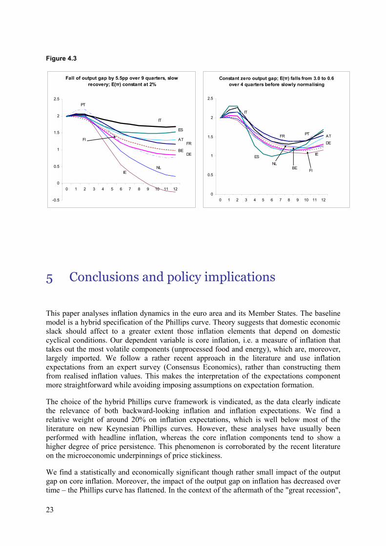
Figure 4.3

Fall of output gap by 5.5pp over 9 quarters, slow recovery; E(π) constant at 2%

-0.5

0

0.5

1

1.5

2

2.5

0 1 2 3 4 5 6 7 8 9 10 11 12

PT

IT

ES

ATFR

BE

FI

DE

NLIE

Constant zero output gap; E(π) falls from 3.0 to 0.6 over 4 quarters before slowly normalising

0

0.5

1

1.5

2

2.5

0 1 2 3 4 5 6 7 8 9 10 11 12

ES

FR

IT

PT AT

DE

IE

BENL

FI

5 Conclusions and policy implications

This paper analyses inflation dynamics in the euro area and its Member States. The baseline model is a hybrid specification of the Phillips curve. Theory suggests that domestic economic slack should affect to a greater extent those inflation elements that depend on domestic cyclical conditions. Our dependent variable is core inflation, i.e. a measure of inflation that takes out the most volatile components (unprocessed food and energy), which are, moreover, largely imported. We follow a rather recent approach in the literature and use inflation expectations from an expert survey (Consensus Economics), rather than constructing them from realised inflation values. This makes the interpretation of the expectations component more straightforward while avoiding imposing assumptions on expectation formation.

The choice of the hybrid Phillips curve framework is vindicated, as the data clearly indicate the relevance of both backward-looking inflation and inflation expectations. We find a relative weight of around 20% on inflation expectations, which is well below most of the literature on new Keynesian Phillips curves. However, these analyses have usually been performed with headline inflation, whereas the core inflation components tend to show a higher degree of price persistence. This phenomenon is corroborated by the recent literature on the microeconomic underpinnings of price stickiness.

We find a statistically and economically significant though rather small impact of the output gap on core inflation. Moreover, the impact of the output gap on inflation has decreased over time – the Phillips curve has flattened. In the context of the aftermath of the "great recession",

23

with large and persistent output gaps, our findings suggest that the observed stability of core inflation can be explained to a large extent by stable inflation expectations, sluggish price adjustment and an only moderate impact of the output gap on inflation.

Despite the recently observed downward rigidity of core inflation our estimates’ support for some non-linear specifications of the Phillips curve is limited. These generally do not fit the data better than the linear baseline specification. The baseline specification also performs well against a number of robustness checks including alternative data sources and estimation methods.

There is some evidence that core inflation in the euro area and Member States is impacted with a lag by commodities price developments, although only indirectly and to a small extent. By contrast, the literature suggests that there is a more sizeable impact of commodity price shocks when considering headline inflation as dependent variable.

Estimated inflation dynamics in the eleven euro area Member States examined cluster quite closely around the Phillips curve relationship estimated for the euro area aggregate. For all Member States, the relative weight of backward-looking inflation is well above that of inflation expectations. Differences across Member States in terms of the relevance of inflation expectations seem to be related to the level of inflation over the past two decades, with Member States having experienced higher average inflation displaying more forward-looking price setting. We interpret this as an indication that firms in countries with higher inflation had stronger incentives to set prices in accordance with inflation expectations, whereas firms in lower-inflation countries had less to lose from a more passive price-setting behaviour.

For all but one Member State, the slope parameter of the Phillips curve has the expected sign and it is statistically significant albeit small. Differences in the steepness of the Phillips curve across Member States correlate with the level of product market rigidity: In more flexible economies the impact of the output gap on inflation appears to be larger. However, this observation is purely statistical and further research in this area is needed. Although the heterogeneity across Member States is not large, the exceptionally large output gap caused by the crisis is one driver of the recently observed inflation differentials across Member States.

Cross-country differences in the responsiveness of core inflation to cyclical conditions could have important policy implications. If symmetric shocks to GDP cause asymmetric inflationary dynamics, divergence in inflation could feed into inflation expectations and, via expected real interest rates, back into growth divergences. Moreover, if inflation dynamics are non-linear with respect to the output gap (for which we do not find compelling evidence, but which is reported in parts of the literature), euro area monetary policy needs to take into account the composition of the aggregate output gap.

Our finding of only mild differences in the Phillips curve parameters across Member States is therefore reassuring in terms of the single monetary policy. Nonetheless, the existence of heterogeneity highlights the role for macroeconomic and possibly structural policies at the level of Member States to help stabilising output and price developments. Over time, as the different parameters of the Phillips curve depend on underlying economic structures (e.g. price stickiness, the level of inflation and product market flexibility), structural adjustment processes in euro area Member States should lead to a further decrease in the heterogeneity of inflation dynamics.

24

This optimistic reading of course supposes that structural reforms are applied in a way that lead to cyclical and structural convergence of euro area economies. It furthermore supposes that inflation differentials across Member States are temporary or, whenever they tend to become persistent as during the first decade of EMU, appropriate macroeconomic and structural policies are deployed to reduce inflation divergence.

Our analysis also highlights some areas for further research. While a lot of research has focussed on the micro-foundations of inflation persistence and inflation expectations, there is scope for looking further into measures of marginal costs, in particular into how structural reforms affect the coefficient on the output gap. We also believe that inflation dynamics after the end of the great moderation deserve further scrutiny. In particular, central banks have taken non-standard measures during the crisis the impact of which on the Phillips curve could be examined further.

25

REFERENCES Aguiar, A. and M.M.F. Martins, (2005), 'Testing the significance of the non-linearity of the Phillips trade-off in the euro area', Empirical economics, 30, 665-691

Baghli, M., C. Cahn and H. Fraisse, (2006), 'Is the inflation-output nexus asymmetric in the euro area?, Banque de France Working Papers NER-E 140

Ball, L. and N.G. Mankiw (1994), 'A sticky-price manifesto' NBER Working Paper No. 4677

Banerjee, R. and N. Batini (2004), 'Inflation dynamics in seven industrialised open economies', mimeo, IMF

Beccarini, A. and D. Gros, (2008), 'At what cost price stability? New evidence about the Phillips curve in Europe and the United States', CEPS Working Document No. 302/September

Benigno, P. and D. López-Salido, (2006), 'Inflation persistence and optimal monetary policy in the euro area', Journal of Money, Credit and Banking, 38(3), 587-614

Buchmann, M. (2009), 'Nonparametric hybrid Phillips curves based on subjective expectations estimates for the euro area', ECB Working Paper No. 1119/December

Calvo, G.A. (1983), 'Staggered prices in a utility-maximizing framework', Journal of Monetary Economics, Vol. 12, Issue 3, 383-398

Curto Millet, F. (2007), 'Inflation expectations, the Phillips Curve and Monetary Policy', Kiel Working Papers No. 1339

Dées, S., Pesaran, M.H., Vanessa Smith, L. and R.P. Smith, (2008), 'Identification of New Keynesian Phillips curves from an international perspective', ECB working paper No. 892.

Dennis, R. (2007), 'Fixing the New Keynesian Phillips Curve', Federal Reserve Bank of San Francisco Economic Letter, 35, 1-3

Dhyne, E., J. Konieczny, J., Rumler, F. and P. Sevestre (2009), 'Price rigidity in the euro area +6– An assessment', Economic Papers No. 380, May

Dolado, J.J., R. Maria-Dolores and M. Naveira (2005), ‘Are monetary-policy reaction functions asymmetric? The role of non-linearity of the Phillips Curve, European Economic Review, 49, 485-503

Dossche, M. (2009), 'Understanding inflation dynamics: Where do we stand?', NBB working paper No. 165, June

Döpke, J., Dovern, J., Fritsche, U. and J. Slacalek, (2008), 'Sticky information Phillips curves: European evidence', ECB working paper No. 930, September

Estrella, A. and J. Fuhrer (2002), 'Dynamic inconsistencies: counterfactual implications of a class of rational expectations models', American Economic Review, 92(4), 1013-1028

European Central Bank (2009), 'The links between economic activity and inflation in the euro area', Monthly Bulletin, September, 54-57.

European Central Bank (2011), 'The link between inflation and the output gap: an illustration based on a Phillips curve framework', Monthly Bulletin, January, 83-84.

Friedman, M. (1968), 'The role of monetary policy', American Economic Review, 58, 1-17

Galí, J. and M. Gertler (1999), 'Inflation dynamics: A structural econometric analysis', Journal of Monetary Economics, 44, 195-222

26

Galí, J., Gertler, M. and D. López-Salido (2001), 'European inflation dynamics', European Economic Review, 45, 1237-1270

Galí, J. and D. López-Salido (2001), 'A new Phillips curve for Spain', Banco de España, Working Paper no. 109

Goodhart, C. and B. Hofmann (2005), 'The Phillips Curve, the IS Curve and monetary transmission: Evidence for the US and the Euro Area', CESifo Economic Studies, 51, 4/2005, 757-775

Gordon, R.J. (2011), 'The History of the Phillips Curve: Consensus and Bifurcation', Economica, Volume 78, Issue 309, 10-50

Gorter, J. (2005), 'Subjective expectations and New Keynesian Phillips Curves in Europe', DNB Working Paper No. 49, August

Heider, M. (2000), 'La non-linearité de la courbe de Phillips de court terme en France et en Allemagne'. Research Paper Université Montesquieu Bordeaux IV

Henzel, S. and T. Wollmershaeuser, (2008), 'The New Keynesian Phillips Curve and the role of expectations: evidence from the IFO World Economic Survey', Economic Modelling, 25, 811-832

Jondeau, E. and H. Le Bihan (2006), 'Testing for the New Keynesian Phillips Curve: Additional International Evidence', Economic Modelling, 22(3), 521-550

Kleibergen, F. and S. Mavroeidis (2009), 'Weak instrument robust tests in GMM and the New Keynesian Phillips Curve', Journal of Business and Economic Statistics, American Statistical Association, 27(3), 293-311

Koske, I. and N. Pain, (2008), 'The usefulness of output gaps for policy analysis', OECD Economics Department Working Papers No. 621

Laxton, D., D. Rose and R. Tetlow (1993), 'Monetary policy, uncertainty and the presumption of linearity', Bank of Canada Technical Report 63.

Lucas, R.E, (1972), 'Expectations and the neutrality of money', Journal of Economic Theory, 4, 103-124

- (1973), 'Some international evidence on ouput-inflation tradeoffs', American Economic Review, 63, 326-334

Mankiw, N. G. and R. Reis (2002), 'Sticky information versus sticky prices: A proposal to replace the New Keynesian Phillips Curve', Quarterly Journal of Economics, 1295-1328

Mankiw, N. G. and R. Reis (2006), 'Pervasive stickiness', American Economic Review, Papers and Proceedings, 164-169

McAdam, P. and A. Willman, (2004), 'Supply, factor shares and inflation persistence: Re-examining euro area New Keynesian Phillips Curves', Oxford Bulleting of Economics and Statistics, 66, Supplement, 637-670

Meier, A. (2010), 'Still minding the gap – Inflation dynamics during episodes of persistent large output gaps', International Monetary Fund Working Paper, No. 10/189

Musso, A., L. Stracca and D. van Dijk (2007), 'Instability and nonlinearity in the euro area Phillips curve', ECB Working Paper No. 811

O'Reilly, G. and K. Whelan (2005), 'Has euro area inflation persistence changed over time?', The Review of Economics and Statistics, 87(4), 709-720

27

Paloviita, M. (2005), 'The role of expectations in euro area inflation dynamics', Bank of Finland Studies E:32

- (2008), 'Estimating open economy Phillips curves for the euro area with directly measured expectations', Bank of Finland Research Discussion Papers 16/2008

Phelps, E.S. (1967), 'Phillips curves, expectations of inflation and optimal unemployment over time', Economica, 34, 254-281

Phillips, A.W. (1958), 'The relation between unemployment and the rate of change of money wage rates in the United Kingdom, 1861-1957', Economica, 25, 283-299

Pyyhtia, I. (1999), 'The Nonlinearity in the Phillips Curve and European Monetary Policy', Bank of Finland, Discussion Paper No. 17/99, November

Roberts, J.M., (1995), 'New Keynesian economics and the Phillips curve', Journal of Money, Credit and Banking, 27(4-)1, 975-984

Rudd, J. and C. Whelan, (2007), 'Modelling inflation dynamics: A critical review of recent research', Journal of Money, Credit and Banking, 39(1), 155-170

Rudd, J. and C. Whelan, (2006), 'Can rational expectations sticky-price models explain inflation dynamics?, American Economic Review, 96(1), 303-320

Rumler, F. (2005), 'Estimates of the open economy New Keynesian Phillips Curve for euro area countries', ECB working paper series No. 496, June

Scheufele, R. (2010), 'Evaluating the German (New Keynesian) Phillips Curve', The North American Journal of Economics and Finance, 21,2, August, 145-164

Schorfheide, F. (2008), 'DSGE model-based estimation of the New Keynesian Phillips Curve', Federal Reserve Bank of Richmond Economic Quarterly 94 (Fall): 397-434

Schumacher, D. and N. Kojucharov (2010), 'The puzzling behaviour of core inflation', Goldman Sachs European Weekly Analyst, No. 10/32

Semmler, W., Greiner, A. and W. Zhang, (2005), 'Monetary and Fiscal Policies in the euro area: Macro modelling, learning and empirics', Elsevier

Smets, F. and R. Wouters, (2005), 'Comparing shocks and frictions in the US and the euro area business cycle models: A Bayesian DSGE approach', Journal of Applied Econometrics, 20,161-183

Staiger, D. and J. Stock (1997), 'Instrumental Variables Regression with Weak Instruments', Econometrica, 65: 557 – 586.

Taylor, J. (1980), 'Aggregate dynamics and staggered contracts', Journal of Political Economy, Vol. 88, pp: 1-23

Vinod, H.D. (2010), 'GMM and OLS estimation and inference for New Keynesian Phillips Curve', Fordhan University, Department of Economics Discussion Paper No. 2010-02

Woodford, M. (2003), 'Interest and Prices', Princeton, N.J.: Princeton University Press

Wooldridge, J.M. (2001), 'Econometrics analysis of cross section and panel data', Cambridge University Press

Zivot, E. and J. Wang (2006), 'Modelling Financial Time Series with S-PLUS', 2nd edition, Springer

28

29

Annex 1 Data set Item * † Source Inflation

HICP headline, headline excluding energy, headline excluding energy and unprocessed food

Eurostat

Remarks: • for DE used CPI excluding energy and seasonal food from Destatis • differing sample length for BE (starts 1991), ES (1992), IE and EL (1995)

Headline CPI, CPI excluding energy and food OECD Inflation expectations Weighted consensus average inflation forecast for current year and year ahead Consensus Economics,

own calculations Remark:

• differing sample length for NL, ES, PT, (starts 1992), EL (1994)

Output Gap

Based on production function (splined annual series)

European Commission (AMECO), own calculations

Remark: • differing sample length for DE (starts 1991), BE, ES, PT (1995), IE (1997), EL (2000)

Based on production function OECD Remark:

• available only for FI, FR, IE, IT and NL (as of 1990), euro area, DE (1991)

HP filtered from quarterly GDP data Eurostat, own calculations

Remark: missing values for DE, IE, EL, ES, LU, PT calculated backwards Unit labour cost RULC and NULC Eurostat, AMECO, own

calculations Remark: missing values for PT,AT, LU, ES, EI, EL constructed backwards using the quarterly average weights for available data and AMECO annual series

Interest rates Three-month money market rate (national rate until euro adoption, then Euribor) Eurostat 10-year benchmark government bong yield Eurostat Commodity prices HWWA price indices for imported commodities denominated in euro EcoWin Crude oil (Brent) expressed in euro EcoWin Real effective exchange rate against 24 industrialised countries

European Commission

Capacity utilisation Joint Business and Consumer Survey

* Geographical coverage includes. EA, AT, BE, DE, ES, FI, FR, EL, IE, IT, NL and PT. Time-span: 1990Q1 to 2010Q4 unless otherwise mentioned † In italics: data used for robustness checks only.

Annex 2 Overview of findings in the related literature N.B.: The table does not aim to be exhaustive. The verbal summary of outcomes focuses on the aspects we deem most relevant in the context of our analysis.

Author(s)

Data Phillips Curve Conclusion

Galí et al. (2001) EA, US Quarterly 1970:1-1998:2 Inflation: GDP deflator Marginal costs: Real Unit Labour Costs (i.e. labour income share)

i) Phelps/Friedman ii) NKPC, with Calvo price setting. iii) hybrid-NKPC, with Calvo price setting.

The hybrid-NKPC fits EA data very well. Inflation dynamics in the EA have a strong forward-looking component. Labour market frictions affect the evolution of marginal costs, and, consequently, inflation in the EA.

Galí and López-Salido(2001)

ES Quarterly 1980:1 – 1998:2 Inflation: GDP deflator Marginal costs: Alternative measures of marginal costs

i) NKPC, with Calvo price setting. ii) hybrid-NKPC, with Calvo price setting.

The hybrid-NKPC fits EA data well. The backward looking component remains significant and large implying a strong degree of price rigidity. Labour market frictions appear to have played a role in shaping the behaviour of marginal cost.

Banerjee and Batini (2004)

UK, FR, IT, DE, CA, NZ, AUS Quarterly 1971:1-2002:1 for the longest series Inflation: GDP deflator Marginal costs: Real Unit Labour Costs (i.e. labour income share)

i) open-economy hybrid-NKPC with different price settings models

The coefficient on the marginal cost is generally small and significant only in FR, UK and NZ. All countries are predominantly forward looking, with a higher degree in DE, NZ, UK and AUS and a smaller degree in IT, FR and CAN. Openness and the price setting method affect the results.

McAdam and Willman (2004)

EA, US Quarterly 1970:1-1997:4 Inflation: GDP deflator; headline HICP Marginal cost: Sector based estimation using a production function.

i) NKPC, with Calvo price setting. ii) hybrid-NKPC, with 'present value' estimate

The preferred hybrid-NKPC using the present value approach has relatively balanced backward- and forward- looking components in the euro area.

Goodhart and Hofmann (2005)

EA, US Quarterly 1982:1- 2001:4 Inflation: headline HICP Marginal cost: Output gap from the area wide model

i) NKPC ii) hybrid-NKPC iii) NKPC and hybrid-NKPC with commodity prices

Both the NKPC and the hybrid-NKPC with commodity prices provide better estimates than the 'simple' forms. Moreover, commodity prices also reduce the magnitude of the forward-looking coefficient in the hybrid-NKPC.

Gorter (2005) FR, DE, IT Quarterly 1991:3-2004:4 Inflation: CPI Marginal cost: Output gap – HP filtered GDP; Real Unit Labour Costs (i.e. labour income share); open-economy measure with input prices indexes Expectations: Consensus Economics

NKPC, with different specifications for marginal costs

The results differ across countries and real marginal costs proxies. For IT, the output gap is a good estimate of marginal costs, whereas for FR and DE the open economy measure performs better. The role of lagged inflation is relevant in DE and IT; in FR the standard forward-looking NKPC effectively captures inflation dynamics. (N.B.: The methodology for assessing the effect of lagged inflation differs from the hybrid-NKPC approach, which makes the comparison with other papers difficult.)

Jondeau and Le Bihan (2005)

EA, DE, FR, IT, UK, US Quarterly 1970:1 to 1999:4 Inflation: GDP deflator Output gap: HP filtered Marginal cost: real ULC (i.e. labour income share)

(i) hybrid-NKPC with one lags and leads (ii) hybrid-NKPC with three lags and leads

The hybrid-NKPC specification with additional lags provides the best fit for continental Europe and, compared to the specification with one lead and lag, a significant decrease in the degree of forward-looking. The authors suggest that the specification with the output gap fits continental European data better; the specification with real unit labour costs fits US and UK data better. The latter also implies a higher weight of the forward-looking component.

O'Reilly and Whelan (2005)

EA Quarterly 1970:1 – 2002:4 Inflation: GDP deflator; headline HICP Marginal cost: Output gap - HP filtered GDP

expectations-augmented PC (Gordon), linear

Strong inflation persistence in the euro area. The values of the estimated coefficients tend to be stable over time.

31

Rumler (2005) EA, AT, BE, DE, ES, FR,

EL, IT, NL Quarterly different start dates (1963-1980) – 2003:2 Inflation: GDP deflator Marginal cost: labour share; domestic and imported intermediate goods prices

i) Hybrid-NKPC ii) Open-economy version(s) of the hybrid-NKPC

Heterogeneity across euro area countries and across specifications for each country. Price persistence consistently matters. The open-economy versions of the hybrid-NKPC provide better estimates on the whole, and then the forward looking coefficient is predominant in most countries.

Semmler et al. (2005) DE, FR, UK, IT Quarterly 1962:1-1999:4 for the longest series Inflation: CPI Marginal cost: Output gap - industrial production index deviation from trend. (For IT, GDP at constant prices.)

i) Phelps/Friedman ii) hybrid-NKPC (system of equations) iii) Time-varying backward-looking PC, with unemployment gap. iv) Time-varying backward-looking PC with supply shocks

The Phelps/Friedman PC is a valid framework to study inflation dynamics in these countries. The hybrid-NKPC offers further insights into the role of the backward and forward looking behaviour of inflation. DE has the strongest forward looking component and FR the lowest. In all countries the output gap has a large coefficient, which has changed over time. Supply shocks are significant in all countries albeit small. The model including supply shocks tends to reinforce the value of the coefficient attached to the output gap.

Benigno and López-Salido (2006)

DE, FR, IT, ES, NL Quarterly 1970:1-1997:1 Inflation: GDP deflator Real marginal costs: Real Unit Labour Costs (i.e. labour income share)

hybrid-NKPC, with Calvo price setting.

DE has a dominant forward-looking component, while in the other countries show a high and significant backward-looking component. Inflation differentials across countries matter for monetary policy.

Musso et al (2007) EA Quarterly 1970:1 - 2005:4 Inflation: GDP deflator; headline HICP Marginal cost: Output gap - first principal component of 6 different measures

(i) expectations-augmented PC (Gordon), linear (ii) expectations-augmented PC (Gordon), time-varying slope and intercept

Strong evidence of shift in the mean of euro area inflation and the slope of the linear PC. No significant evidence of non-linearity of the curve.

32

Beccarini and Gros (2008)

EA, US Quarterly 1996:1 to 2008:1 Inflation: headline HICP; core inflation Marginal cost: Output gap - HP filtered GDP

(i) expectations-augmented PC (Gordon) with oil prices for headline (ii) expectations-augmented PC (Gordon) with oil prices for core

Using headline inflation, the mean and the volatility of inflation appear to be higher in the past decade. The impact of oil prices is more persistent in the EA, and the slope coefficient is higher in the EA than in the US. Oil price increases affect little the core inflation estimate of the PC, and inflation persistence is higher than in the headline specification with lower impact of the output gap.

Dées et al (2008) EA, US, Group estimates (26 countries) Quarterly 1980:II-2003:III Inflation: headline HICP Marginal cost: Output gap - GVAR estimation of steady state

(i) hybrid PC (ii) Open-economy hybrid-NKPC extended with domestic interest rates, foreign output gap and foreign, inflation

For the euro area, stronger weight on forward-looking than backward-looking inflation. Slope coefficient only correctly signed in version (ii). The weakness of domestic determinants of inflation in the euro area might reflect the aggregation of heterogeneous countries.

Henzel and Wollmershäuser (2008)

DE, FR, IT, EA, UK, US 1993:1 to 2004:2 Inflation: headline HICP Marginal cost: Real Unit Labour Costs; OECD output gap. Expectations: Ifo World Economic Survey (WES) (quantified).

i) NKPC ii) hybrid- NKPC

Preference for the hybrid-NKPC specification. The backward-looking coefficient is dominant in DE and IT, but not in FR. For the euro area, backward- and forward-looking terms are balanced. The output gap provides better estimates than the real unit labour costs.

Paloviita (2008) Annual, 1981-2006 (1990-2006 for pooled estimates); Inflation: CPI Output gap: HP filtered Expectations: OECD forecasts; Consensus (in shorter sample)

(i) NKPC (ii) Hybrid PC

In the closed-economy hybrid NKPC has similar proportions of forward- and backward looking (γb = 0.44 in the estimation with pooled data and 0.54 in the estimation with aggregate data; γf is fixed at (1- γb)).

33

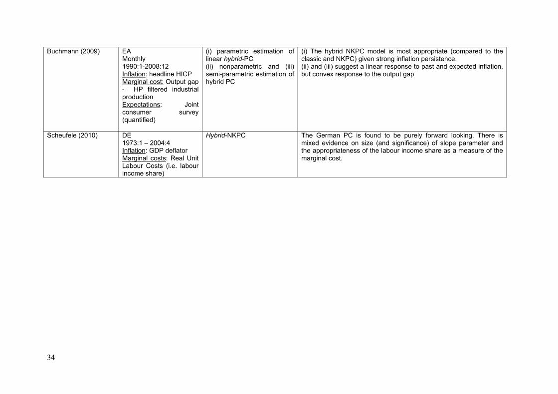
34

Buchmann (2009) EA Monthly 1990:1-2008:12 Inflation: headline HICP Marginal cost: Output gap - HP filtered industrial production Expectations: Joint consumer survey (quantified)

(i) parametric estimation of linear hybrid-PC (ii) nonparametric and (iii) semi-parametric estimation of hybrid PC

(i) The hybrid NKPC model is most appropriate (compared to the classic and NKPC) given strong inflation persistence. (ii) and (iii) suggest a linear response to past and expected inflation, but convex response to the output gap

Scheufele (2010)

DE 1973:1 – 2004:4 Inflation: GDP deflator Marginal costs: Real Unit Labour Costs (i.e. labour income share)

Hybrid-NKPC

The German PC is found to be purely forward looking. There is mixed evidence on size (and significance) of slope parameter and the appropriateness of the labour income share as a measure of the marginal cost.

Annex 3

γb γf λ R² J-stat sample instruments

Belgium 0.342* 0.594*** 0.250*** 0.601 0.042 1995q2 - 2010q4 cons(-1) cap ishort ishort(-1) ygap(-1)

Germany 0.548*** 0.469*** 0.096*** 0.886 0.062 1991q2 - 2010q3 cons(-1) cons(-2) ilong ilong(-1) ygap(-1)

Ireland 0.481*** 0.485*** 0.162*** 0.88 0.000 1997q2 - 2010Q3 cons(-1) cons(-2) ygap(-1)

Spain 1.120*** -0.109 0.115 0.592 0.098 1995q2 - 2010q3 cons(-1) ishort ishort(-1) brent brent(-2) ygap(-1)

France 0.571*** 0.404*** 0.087*** 0.767 0.026 1991q2 - 2010q3 cons(-1) coagri ilong ygap(-1)

Italy 0.237*** 0.856*** 0.120*** 0.905 0.106 1991q4 -2010q1 cons(-1) cons(-2) ishort ishort(-1) ishort(-2) coxe coxe(-2) coxe(-3) brent brent(-1) cap cap(-1) ygap(-1)

Netherlands 0.829*** 0.145** 0.073** 0.807 0.073 1992q3 - 2010q3 cons(-1) cons(-2) ilong ilong(-2) ilong (-3) brent ygap(-1)

Austria 0.245 0.763*** 0.125*** 0.668 0.028 1996q2 - 2010q4 cons(-1) ishort d(cap) ygap(-1)

Portugal 0.14 0.848*** 0.164** 0.691 0.099 1995q2 - 2010q3 cons(-1) cons(-2) ishort ishort(-1) rulc ygap(-1)

Finland 0.539* 0.350 0.029 0.773 0.000 1991q2 - 2010q3 cons(-1) cons(-2) brent ygap(-1)

Phillips curve estimates with headline inflation as dependent variable