the implications of climate policy for avoided impacts on

Available online at www.sciencedirect.com

Procedia Environmental Sciences 4 (2011) 112–xxxProcedia Environmental Sciences 6 (2011) 112–121

1878-0296 © 2011 Published by Elsevierdoi:10.1016/j.proenv.2011.05.012

Earth System Science 2010: Global Change, Climate and People

The implications of climate policy for avoided impacts on water scarcity

Simon N. Goslinga*, Nigel W. Arnella, Jason A. Loweb aWalker Institute for Climate System Research, University of Reading, Reading RG6 6AR, United Kingdom

bMet Office Hadley Centre, Exeter EX1 3PB, United Kingdom

Abstract

We present simulations of the impact of climate change on global water scarcity for five greenhouse gas emissions mitigation policy scenarios and compare them with a business-as-usual emissions scenario. A global water scarcity model is driven by climate change projections from 21 global climate models (GCMs). An aggressive policy scenario that gives a 50% chance of avoiding a 2°C global-mean temperature rise from pre-industrial times could avoid almost 40% of the business as usual global impacts by 2100. However, mitigation policy does not completely eliminate the impacts of climate change. For any given GCM, the avoided impacts are affected more by the year at which emissions peak than to the rate at which emissions are subsequently reduced and the uncertainty across the 21 forcing GCMs is large.

© 2011 Published by Elsevier Ltd. Selection under responsibility of QUEST. Key Words: Climate change; water scarcity; water resources; climate policy; avoided impacts; uncertainty

1. Introduction

Recent climate change impacts assessments indicate that climate change will have generally negative impacts onvarious sectors including, for instance, water scarcity [1], agriculture and food production [2], human health [3,4], and ecosystems and biodiversity [5].

An increasingly common opinion is that to avoid ‘dangerous’ climate change, global-mean warming needs to be limited to below 2°C above pre-industrial levels. This is reflected in, for example, the EU’s policy target for EU-wide and international climate change mitigation negotiations of 2°C global-mean warming by 2100. Information on the potential impacts that climate change will have for different amounts of global-mean warming is therefore of considerable importance to policy-makers. Furthermore, the impacts associated with different climate change mitigation policies relative to ‘business-as-usual scenarios’ can be used to better-inform the decision-making process.

* Corresponding author. Tel.: +44 (0) 118 378 8225; fax: +44 (0) 118 378 8316.E-mail address: [email protected] .

Open access under CC BY-NC-ND license.

Open access under CC BY-NC-ND license.

http://creativecommons.org/licenses/by-nc-nd/3.0/

http://creativecommons.org/licenses/by-nc-nd/3.0/

Simon N. Gosling et al. / Procedia Environmental Sciences 6 (2011) 112–121 113

g

g ( )

The aim of this paper is to assess the potential impacts of climate change on global water scarcity that could be avoided by a set of defined climate policies, one of which includes an aggressive mitigation scenario that gives a 50% chance of avoiding a 2°C global-mean temperature rise from pre-industrial times. The paper uses an existing climate change impacts assessment model with climate scenarios representing the effects of a range of different climate policies, and compares impacts under a business-as-usual climate with those under the specified policies.

2. Methods

2.1. Climate change scenarios

We compare climate change policies representing different dates at which carbon dioxide (CO2) emissions peak, rates at which emissions decline, and emissions floors, and compare them with an SRES [6] A1B business-as-usual emissions scenario. The emissions scenarios are summarised in Table 1 and Figure 1(a). For a given emissions scenario, global temperature change was estimated using a simple climate model; MAGICC [7], run with a large number of parameter combinations. Figure 1(b) shows the global-mean temperature change for each scenario, based upon the median estimate of the ensemble produced by the parameter perturbations. The A1B-2016-5-L policy scenario gives a 50% chance, based upon the parameter perturbations, of avoiding a 2°C global-mean temperature rise from pre-industrial times [7].

Scenarios for change in mean monthly climate (temperature, precipitation, vapour pressure and net radiation) were derived by pattern-scaling and downscaling output from 21 global climate models (GCMs) used in the IPCC AR4, using the ClimGen package [8]. The pattern-scaling approach was used to construct climate scenarios for a given change in global-mean temperature T, as simulated using the MAGICC simple climate model for the emissions scenarios presented in Table 1. The pattern for each GCM was constructed by fitting a regression, for each month, variable and GCM grid cell, between climate variable and global mean temperature, in order to estimate change in climate per degree change in global-mean temperature. The pattern-scaling approach assumes that the relationship between global temperature change and local climate response is linear and invariant. The pattern-scaling was performed at the original GCM grid resolution and then interpolated statistically to 0.5° x 0.5° resolution. Baseline climate is represented by the period 1961-1990, with monthly climate data taken from the UEA CRU-TS3 data set.

Table 1. The climate change policy emissions scenarios

Scenario name Pathway to peak Date of peak Rate of decline in emissions post-peak Emissions floor

A1B-2016-2-H A1B 2016 2% per year High

A1B-2016-4-L A1B 2016 4% per year Low


A1B-2030-2-H A1B 2030 2% per year High


114 Simon N. Gosling et al. / Procedia Environmental Sciences 6 (2011) 112–121

g ( )

Figure 1. The climate change emissions scenarios (a), and global-mean temperature rise from pre-industrial times (b).

Table 2. Regional and global population through the 21st century under the SRES A1B scenario, as implemented in IMAGE v2.3 [13].

Region Population (millions)

2000 2030 2050 2080 2100

North Africa 174 245 266 269 252

Western Africa 238 385 447 481 455

Central Africa 85 148 178 194 183

Eastern Africa 145 252 311 343 329

Western Indian Ocean 19 32 39 40 37

Southern Africa 152 182 191 206 195

South Asia 1433 1963 2084 1918 1600

Southeast Asia 523 682 723 656 556

NW Pacific and East Asia 1508 1624 1537 1286 1044

Central Asia 57 78 86 87 78

Australia and New Zealand 23 29 34 32 29

South Pacific 7 12 15 16 14

Western Europe 394 415 431 427 391

Central Europe 198 211 205 175 158

Eastern Europe 227 213 198 179 170

Arabian Peninsula 48 104 146 194 198

Mashriq 53 90 104 108 97

Canada 31 37 39 40 38

US 284 361 403 414 387

Caribbean 37 44 44 42 39

Meso-America 135 187 206 208 191

Brasil 169 212 224 211 190

South America 131 180 201 209 195

World 6070 7686 8110 7734 6822


2.2. The climate change impacts assessment model

Mac-PDM is a global hydrological model (GHM) that simulates river runoff across the world at a spatial resolution of 0.5° x 0.5°. A detailed description of the model is given by Gosling and Arnell [9] and a recent inter-model comparison exercise shows that the model performs as well as other GHMs [10]. In brief, Mac-PDM calculates the water balance in each 0.5° x 0.5° cell on a daily basis, treating each cell as an independent catchment, generating river runoff from precipitation falling on the portion of the cell that is saturated, and by drainage from water stored in the soil. The model parameters are not calibrated - model parameters describing soil and vegetation characteristics are taken from spatial data sets. Mac-PDM was forced with the A1B and policy pattern-scaled climate change scenarios described previously. The simulations were performed on the University of Reading Campus Grid by high throughput computing (HTC, [1]).

We used average annual runoff simulated by Mac-PDM to characterise available water resources using the water resources model described in Arnell [11]. It is necessary to define an indicator of pressure on water resources for the model. Here we used the amount of water resources available per person, expressed as m3/capita/year. This index was used by the PAGE study [12]. The water resources model assumes that watersheds with less than 1000 m3/capita/year experience water scarcity. Therefore populations that move into this scarcity category are considered to experience an increase in water resources scarcity. However, some populations are already within the water scarcity category, because present-day resources per capita are less than 1000 m3/capita/year. Therefore a more complicated measure combines the number of people who move into (out of) this scarcity category with the numbers of people already in the scarcity category who experience an increase (decrease) in water scarcity with climate change. The key element here is to define what characterises a ‘significant’ change in runoff, and hence water scarcity. The water resources model assumes a ‘significant’ change in runoff, and hence water scarcity, occurs when the percentage change in mean annual runoff is more than the standard deviation of 30-year mean annual runoff due to natural multi-decadal climatic variability. Hence the water resources model calculates the millions of people at increased risk to water resources scarcity with climate change as the sum of the populations that move into the scarcity category (resources less than 1000 m3/capita/year) and the numbers of people already in the scarcity category who experience an increase in water scarcity.

The population projections required for the water scarcity calculations are assumed to follow the SRES A1B scenario, as implemented in IMAGE v2.3 [13] for all policy emissions scenarios and the business as usual emissions scenario. Table 2 shows regional population through the 21st century for this scenario. Important to note is that the population projection shows a decline in global population following a peak in 2050, and defines a global population slightly less than that under most other projections (such as UN medium-fertility population projections). Water scarcity is calculated for the 23 regions displayed in Table 2 and for the entire world.

3. Results

3.1. Regional avoided impacts

Figure 2 shows the regional absolute avoided impacts (millions of people) under the A1B-2016-5-L policy emissions scenario at 2100. This demonstrates that for an emissions policy that gives a 50% chance of avoiding a 2°C global-mean temperature rise from pre-industrial times (A1B-2016-5-L), policy generally has a positive effect. For some regions, there is consensus across the majority of GCMs that climate change does not affect water scarcity at all (e.g. Australia and New Zealand and Brazil). The regions that present the largest avoided impacts consistently across the range of 21 GCMs include North Africa, NW Pacific and East Asia, and South Asia. However, there is considerable variation across GCMs of the magnitude of these avoided impacts. For instance, the magnitude of avoided impacts range between 10-90 million (North Africa), 0-80 million (NW Pacific and East Asia) and 30-90 million (South Asia), across all 21 GCMs. Whilst there is considerable variation across the 21 GCMs, generally the majority of GCMs are in agreement that emissions policy avoids some amount of increases in water scarcity with climate change, relative to the business as usual scenario, for these regions.


113

In a minor number of cases, the emissions mitigation policy is associated with a relatively small (<5 million people) increase in water scarcity relative to the business as usual scenario, denoted by the red shaded regions (e.g. South America for the two UKMO GCMs and two NCAR GCMs). This is because with these GCMs and regions, the simulated climate under the business as usual scenario presents an increase in precipitation which is greater than that simulated under the policy scenario – since some parts of the those regions also experience similar reductions in precipitation with climate change under both policy and business as usual scenarios, the net effect is that water scarcity slightly increases with the policy scenario relative to the business as usual scenario. However, the majority of GCMs show that the avoided impacts are positive for these regions.

The absolute avoided impacts presented in Figure 2 are informing but another important measure is the relative avoided impacts, where the avoided impacts under the policy scenario are expressed as a percentage of the impacts under the business as usual emissions scenario. This is a useful indicator because it gives a standardised measure of the magnitude of the ‘benefit’ realised by a given policy scenario and means that the regional avoided impacts can be compared.

Figure 3 shows the relative regional avoided impacts under the A1B-2016-5-L policy scenario at 2100 for the 21 GCMs. Similar to the patterns for absolute impacts, NW Pacific and East Asia is one of the regions that experience the largest benefits of emissions policy scenario in terms of reduced increases in water scarcity. Typically >60% of business as usual impacts are avoided under the policy scenario here. Whilst Figure 2 shows Eastern Europe is associated with modest avoided absolute impacts (typically <20 million for any given GCM), Figure 3 shows that the relative benefits are more substantial here (typically >40%).

A small number of GCMs present negative relative benefits for South America, e.g. the two NCAR and UKMO GCMs. However, the majority of GCMs show a positive avoided impact for this region. Furthermore, the absolute magnitude of the avoided impact is greater than -5 million (Figure 2) for these GCMs, which is small relative to the benefits presented for the same region by the other GCMs. Nevertheless, this result can not be ignored because in the present analysis, it is assumed that all the GCMs are equally credible (although they are not completely independent). This is a reasonable assumption at present because of the challenge in defining appropriate measures of relative performance [14], but this does require further investigation.

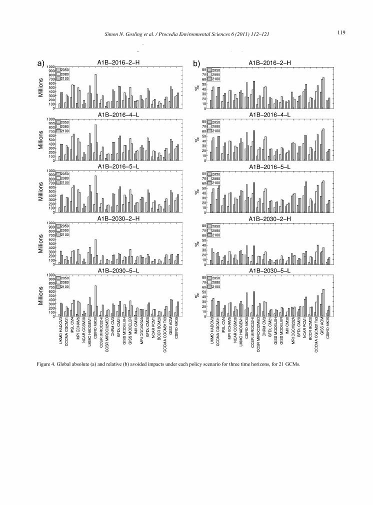
3.2. Global avoided impacts

Figure 4(a) shows the global absolute avoided impacts under each of the five policy scenarios for three time horizons, across the 21 GCMs. For a given GCM, the avoided impacts are greater with the policy scenarios where emissions peak in 2016 than they are where emissions peak in 2030. For instance, with UKMO HADCM3 at 2100 each of the three policy scenarios with a 2016 emissions peak are associated with an avoided increase in global water scarcity of around 400 million people. The avoided impacts with the two policy scenarios where emissions peak in 2030 are between 200 and 300 million. Within the 2016-peak policies the differences in avoided impacts between the three policy scenarios are minor and the same is true for the two 2030-peak scenarios. This means the year at which emissions reductions begin has a greater effect on avoided impacts than the annual rate at which emissions are reduced.


Figure 2. Regional absolute avoided impacts (millions of people) under the A1B-2016-5-L emissions policy scenario at 2100, for 21 GCMs. ‘NI’ denotes ‘no impact’, i.e. under the A1B emissions scenario there is no increase or decrease in water scarcity so avoided impacts are not calculated here.

The magnitudes of global absolute avoided impacts are greater in 2080 and 2100 than they are in 2050. It therefore takes at least 50 years from when emissions reductions begin for any sizeable benefits to be realised. For example, taking the A1B-2016-5-L scenario, with some GCMs the avoided impacts at 2080 are over double the avoided impacts at 2050, e.g. GISS AOM, GFDL CM21 and CNRM CM3. Water scarcity is a function of climate change and socioeconomics, which is why with some GCMs even though global-mean temperature is higher in 2100 than 2080, avoided impacts are not necessarily greater in 2100 than in 2080, e.g. see the avoided impacts associated with the UKMO HADGEM1 and CSIRO MK35 GCMs in Figure 4(a). Global total population is lower in 2100 than in 2080 under the A1B socioeconomic scenario and given that water scarcity is calculated from a per capita threshold of 1000m3/year, the increase in avoided impacts with global-mean temperature is non-linear.

The global relative avoided impacts in water scarcity of the 5 policy scenarios are presented in Figure 4(b) for three time horizons. Similar to the conclusions drawn from Figure 4(a), the year at which emissions reductions begin has a greater effect on avoided impacts than the annual rate at which emissions are reduced. With some GCMs the relative benefits of emissions policy are large, CCSR MIROC32HI and GISS AOM present avoided impacts of over 60% of the A1B impacts at 2100 with the 2016-5-L policy, for instance.

Whilst the year of emissions peak is shown to be an important factor on the magnitude of the relative and absolute avoided impact, more important is the choice of GCM. Figure 4(a) and Figure 4(b) show that the range across all 21 GCMs of avoided impacts for any given policy scenario and year is greater than the range across policy scenarios for any given GCM and year. Therefore the magnitude of the avoided impacts is mostly dependent upon GCM.


Figure 3. Regional relative avoided impacts (expressed as a percentage of the impacts under the A1B emissions scenario) under the A1B-2016-5-L emissions scenario at 2100. ‘NI’ denotes ‘no impact’, i.e. under the A1B emissions scenario there is no increase or decrease in water scarcity so avoided impacts are not calculated here.

Figure 5 summaries the magnitude of global relative avoided impacts under the A1B-2016-5-L policy scenario – the ensemble mean and range across the 21 GCMs is plotted. This aggressive mitigation policy scenario could avoid around 20% of the business as usual impacts by 2050, 35% by 2080 and almost 40% by 2100. However, climate change continues to have an impact on water scarcity, even with stringent mitigation. Whilst the uncertainty range across GCMs is large (20-65% in 2100), there is consensus across all 21 GCMs that the mitigation policy avoids, to some extent, the impacts of climate change on water scarcity relative to the business as usual scenario.


g

g ( )

Figure 4. Global absolute (a) and relative (b) avoided impacts under each policy scenario for three time horizons, for 21 GCMs.


Figure 5. The ensemble mean (horizontal lines) and the range (shaded) across all 21 GCMs of global relative avoided impacts under the A1B-2016-5-L policy scenario for three time horizons.

4. Conclusions

Our simulations have shown that for an aggressive emissions mitigation policy scenario that gives a 50% chance of avoiding a 2°C global-mean temperature rise from pre-industrial times (A1B-2016-5-L), that there is consensus across the majority of 21 forcing GCMs that climate change either does not affect water scarcity at all (e.g. Australia and New Zealand and Brazil) or that some of the impacts simulated under a business as usual scenario could be avoided. North Africa, NW Pacific and East Asia, and South Asia present the largest avoided impacts. Whilst there is consensus across the 21 GCMs that some impacts can be avoided, there is considerable variation across GCMs of the magnitude of these avoided impacts. The A1B-2016-5-L policy scenario could avoid around 20% of the business as usual global-scale impacts of climate change on water scarcity by 2050, 35% by 2080 and almost 40% by 2100. In spite of the aggressive nature of this mitigation scenario, however, some residual impacts remain, i.e. 100% of the impacts of climate change can not be avoided. An important conclusion for policy-making is that for any given GCM, the avoided impacts are affected more by the year at which emissions peak than to the rate at which emissions are subsequently reduced. However, given that the uncertainty in the magnitude of avoided impacts across GCMs is large, the prioritising and weighting of GCM-dependent impacts is a challenge for the future.

Acknowledgments

This work was supported by the AVOID programme (funded by DECC and Defra under contract DECC/Defra GA0215) and a grant from the Natural Environment Research Council (NERC), under the QUEST programme (grant number NE/E001890/1). Thank you to Dan Bretherton (ESSC, University of Reading, UK), University of Reading IT Services and the entire University of Reading Campus Grid team for their support in setting-up Mac-PDM to run by high throughput computing on the University of Reading Campus Grid. ClimGen was developed by Tim Osborn at the Climatic Research Unit (CRU) at the University of East Anglia (UEA), UK.

References

[1] Gosling SN, Bretherton D, Haines K, Arnell NW. Global Hydrology Modelling and Uncertainty: Running Multiple Ensembles with a Campus Grid. Philosophical Transactions of the Royal Society A. 2010;368: 1-17, doi:10.1098/rsta.2010.0164

[2] Challinor AJ, Wheeler TR. Use of a crop model ensemble to quantify CO2 stimulation of water-stressed and well-watered crops. Agricultural and Forest Meteorology 2008;148: 1062-1077.


g

g ( )

[3] Gosling SN, Lowe JA, McGregor GR. Climate change and heat-related mortality in six cities Part 2: Climate model evaluation, sensitivity analysis, and estimation of future impacts. International Journal of Biometeorology 2009;53: 31-51. doi:10.1007/s00484-008-0189-9

[4] Gosling SN, Lowe JA, McGregor GR. Projected impacts on heat-related mortality from changes in the mean and variability of temperature with climate change. IOP Conference Series: Earth and Environmental Science 2009:6: 142010. doi:10.1088/1755-1307/6/14/142010

[5] Veron JEN, Hoegh-Guldberg O, Lenton TM, Lough JM, Obura DO, Pearce-Kelly P, Sheppard CRC, Spalding M, Stafford-Smith MG, Rogers AD. The coral reef crisis: The critical importance of <350 ppm CO2. Marine Pollution Bulletin 2009;58: 1428-1436.

[6] Naki enovi N, Swart R (Eds.) Special Report on Emission Scenarios. Cambridge: Cambridge University Press, 2000. [7] Gohar L, Lowe JA. Summary of the emissions mitigation scenarios. AVOID Workstream 1/Deliverable 1/Report 2. Met Office Hadley

Centre, 2009. [8] Todd MC, Taylor RG, Osborn T, Kingston DG, Arnell NW, Gosling SN. Quantifying the impact of climate change on water resources at the

basin scale on five continents – a unified approach. Hydrol. Earth Syst. Sci. Discuss., under review. [9] Gosling SN, Arnell, NW. Simulating current global river runoff with a global hydrological model: model revisions, validation and sensitivity

analysis. Hydrological Processes, in press, doi: 10.1002/hyp.7727 [10] Haddeland I, Clark C, Franssen W, Ludwig F, Voß F, Arnell NW, Bertrand N, Best S, Folwell S, Gerten D, Gomes S, Gosling SN,

Hagemann S, Hanasaki N, Harding N, Heinke J, Kabat P, Koirala S, Polcher J, Stacke T, Viterbo P, Weedon G, Yeh P. Multi-Model Estimate of the Global Water Balance: Setup and First Results. Journal of Hydrometeorology, under review.

[11] Arnell NW. Climate change and global water resources: SRES emissions and socio-economic scenarios. Global Environmental Change 2004;14: 31-52

[12] Revenga C, Brunner J, Henninger N, Kassem K, Payne N. Pilot Analysis of Global Ecosystems: Freshwater Ecosystems. Washington, DC: World Resources Institute and Worldwatch Institute, 2000.

[13] Van Vuuren DP, den Elzen MGJ., Lucas PL, Eickhout B, Strengers BJ, van Ruijven B, Wonink S, van Houdt R. Stabilizing greenhouse gas concentrations at low levels: an assessment of reduction strategies and costs. Climatic Change 2007;81: 119-159.

[14] Gleckler PJ, Taylor KE, Doutriaux C. Performance metrics for climate models. Journal of Geophysical Research 2008; 113: D06104.

the implications of climate policy for avoided impacts on

Documents