the implementation of a texas hydrologic information system by
TRANSCRIPT

The Implementation of a Texas
Hydrologic Information System
by
Bryan Jacob Enslein, M.S.E.
David R. Maidment, Ph.D.
May 2009
CENTER FOR RESEARCH IN WATER RESOURCES
Bureau of Engineering Research • The University of Texas at Austin J.J. Pickle Research Campus • Austin, TX 78712-4497
This document is available online via World Wide Web at
http://www.crwr.utexas.edu/online.shtml

Dedication
I dedicate this thesis to my family and friends who are always so quick with words of
encouragement.
iii
Acknowledgements
I would like to thank my advisor, Dr. David Maidment, for his constant guidance,
vision and energy and Tim Whiteaker for his patience while assisting my work on the
Hydrologic Information System. I would also like to thank the Texas Natural Resources
Information System and those at the Texas Water Development Board, especially Jorge
Izaguirre and Ruben Solis, for their support.
May 8, 2009

iv
Abstract
The Implementation of a Texas
Hydrologic Information System
Bryan Jacob Enslein, M.S.E.
The University of Texas at Austin, 2009
Supervisor: David R. Maidment
Work has been successfully performed by the Consortium of Universities for the
Advancement of Hydrologic Science, Inc. (CUAHSI) to synthesize the nation’s
hydrologic data. Through the building of a national Hydrologic Information System
(HIS), the organization has demonstrated a successful structure that promotes data
sharing. Using this national model, The Center for Research in Water Resource (CRWR),
in conjunction with the Texas National Resource Information System (TNRIS), has
developed and implemented a Texas HIS that facilitates statewide and regional
hydrologic data sources. Advancements have been made in data loading, access, and
cataloging that apply to national and statewide project implementation.
v
Table of Contents
List of Tables ....................................................................................................... viii
List of Figures ........................................................................................................ ix
List of Acronyms .....................................................................................................x
1 INTRODUCTION 1
1.1 The HIS Project...............................................................................................3
1.2 Building an HIS ..............................................................................................4
1.3 Building a State HIS .......................................................................................5
1.4 Thesis Objectives ............................................................................................7
2 LITERATURE REVIEW 8 2.1.1 Hydroinformatics ...................................................................................8
2.2 Similar HIS Efforts .........................................................................................8
2.2.1 The GeoBrain Online Analysis System .................................................9
2.2.2 Water Management Information System .............................................11
3 METHODOLOGY 14
3.1 The HIS Model .............................................................................................14
3.2 Data Housing ................................................................................................16
3.2.1 The Observations Data Model .............................................................16
3.2.2 The Observations Data Model Structure ..............................................19
3.2.3 Data Housing Methods ........................................................................21
3.2.4 Hybrid Web Services ...........................................................................22
3.3 Data Upload ..................................................................................................24
3.3.1 SQL Server Integrated Services Data Loading ....................................24
3.3.2 Loading Data with the ODM Data Loader ..........................................27
3.3.3 Comparison of the ODMDL and SSIS Data Loading Methods ..........29

vi
3.4 Data Publication ............................................................................................31
3.4.1 WaterOneFlow Services and the ODM ...............................................31
3.4.2 WaterOneFlow and Web Service Definition Language ......................32
3.4.3 Web Mapping Services ........................................................................35
3.4.4 Web Feature Services ..........................................................................36
3.4.5 Web Feature and Web Mapping Services Within the HIS ..................36
3.4.6 Data Registry .......................................................................................38
3.5 Data Discovery ..............................................................................................41
3.5.1 HydroSeek............................................................................................41
3.5.2 TCEQ GEMSS Viewer ........................................................................43
3.5.3 HydroExcel ..........................................................................................45
3.5.4 Data.Crwr Web Registry ......................................................................47
3.5.5 User Experience ...................................................................................49
4 CASE STUDY OF THE TEXAS WATER DEVELOPMENT BOARD DATA PUBLICATION PROCESS 50
4.1 TWDB Data Background ..............................................................................52
4.1.1 TWDB Data Structure ..........................................................................52
4.1.2 TWDB Data Format .............................................................................53
4.2 Distinct ODM Data Services ........................................................................57
4.2.1 TWDB SSIS Loading Process .............................................................59
4.2.2 Observation Data Model Data Loader Loading Process ......................65

vii
4.3 Data Publishing .............................................................................................67
5 CONCLUSIONS 69
5.1 Recommendations for Future Research ........................................................72
APPENDIX A: NATIONAL AND ACADEMIC DATA SETS 75
APPENDIX B: ODM 1.1 FIELDS AND CONTROLLED VOCABULARIES 78
APPENDIX C: SSIS DATA LOADING TUTORIAL 111
APPENDIX D: SSIS DATA LOADING TUTORIAL 125 Installing an ODM database onto SQL Server: ..........................................126
Loading Data into the ODM .......................................................................130
GLOSSARY: 142
BIBLIOGRAPHY 143
VITA 145

viii
List of Tables
Table 3-1 Primary ODM Tables ....................................................................................... 19 Table 3-2 ODM Table Loading Order (Jantzen, 2007) .................................................... 26 Table 3-3 Texas HIS Registered WSDLs ......................................................................... 34 Table 3-4 MySelect Table Fields ...................................................................................... 37 Table 3-5 Salinity Thematic Series ................................................................................... 41 Table 4-1 TWDB Variable Codes ..................................................................................... 63 Table 0-1 National and International Data Sources .......................................................... 75 Table 0-2 Academic Data Sources .................................................................................... 76
ix
List of Figures
Figure 1-1 Texas HIS Data Portal ....................................................................................... 3 Figure 1-2 Scales of Hydrologic Data (Jantzen, 2007) ....................................................... 6 Figure 2-1 GeOnAS User Interface (Han et al, 2008) ........................................................ 9 Figure 2-2 GeOnAS Architecture (Center for Spatial Information Science and System) 10 Figure 2-3 WMIS User Search Interface .......................................................................... 12 Figure 2-4 WMIS Mapping Interface ............................................................................... 13 Figure 3-1 The HIS Model ................................................................................................ 14 Figure 3-2 The Observations Data Model 1.1 (Tarboton et al, 2008) .............................. 18 Figure 3-3 Simplified ODM Representation ..................................................................... 20 Figure 3-4 Centralized vs. Distributed System ................................................................. 22 Figure 3-5 TCOON Hybrid Service .................................................................................. 23 Figure 3-6 SSIS Field Mapping ........................................................................................ 27 Figure 3-7 ODM Data Loader 1.1 ..................................................................................... 29 Figure 3-8 Water Markup Language................................................................................. 32 Figure 3-9 WSDL Data Request ....................................................................................... 33 Figure 3-10 Web Mapping Service in ArcExplorer .......................................................... 35 Figure 3-11 Data.Crwr Texas HIS Data Service Registry ................................................ 38 Figure 3-12 Salinity Thematic Layer ................................................................................ 40 Figure 3-13 HydroTagger (www.hydrotagger.org) ......................................................... 42 Figure 3-14 HydroSeek (www.hydroseek.org) ................................................................. 43 Figure 3-15 GEMSS Viewer (www.waterdatafortexas.org) ............................................. 44 Figure 3-16 WMS GEMS Display .................................................................................... 45 Figure 3-17 TWDB Tides KML File ................................................................................ 46 Figure 3-18 HydroExcel Statistics and Charts .................................................................. 47 Figure 3-19 TCEQ TRACS Dynamic Map ...................................................................... 48 Figure 3-20 User v Provider Perspective .......................................................................... 49 Figure 4-1 TWDB Field Study Locations ......................................................................... 50 Figure 4-2 Datasonde ........................................................................................................ 51 Figure 4-3 TWDB Field Studies Data Housing Structure ................................................ 53 Figure 4-4 Example TWDB Readme File ........................................................................ 54 Figure 4-5 Sample TWDB Datasondes Data File ............................................................. 55 Figure 4-6 TWDB Water Quality Data ............................................................................. 56 Figure 4-7 TWDB Tides Sample Data.............................................................................. 57 Figure 4-8 HIS Data Hierarchy ......................................................................................... 58 Figure 4-9 SSIS Data Loading Process ............................................................................. 59 Figure 4-10 SSIS Connection Manager ............................................................................ 60 Figure 4-11 TWDB Datasondes ODM Sites Table .......................................................... 63 Figure 4-12 TWDB Tides Sites ........................................................................................ 65 Figure 4-13 ODMDL of TWDB Tide Data Values .......................................................... 66 Figure 4-14 TWDB Datasondes Data.CRWR Registry Page ........................................... 67

x
List of Acronyms
CSW: Catalogue Services for Web
CRWR: Center for Research in Water Resources
CUAHSI: Consortium of University for the Advancement of Hydrologic Science Inc.
EPA: Environmental Protection Agency
GEMS: Geospatial Emergency Management Support System
GeOnAs: GeoBrain Online Analysis System
HIS: Hydrologic Information System
NOAA: National Oceanic and Atmospheric Agency
ODM: Observation Data Model
ODM DL: Observation Data Model Data Loader
OGC: Open Geospatial Consortium Inc.
SSIS: SQL Server Integrated Services
TCEQ: Texas Commission on Environmental Quality
TCOON: Texas Coastal Ocean Observation Network
TNRIS: Texas Natural Resources Information System
TRACS: TCEQ Regulatory Activities and Compliance System
TPWD: Texas Parks and Wildlife Department
TWDB: Texas Water Development Board
USGS: United States Geologic Survey
WaterML: Water Markup Language

xi
WCS: Web Cover Service
WFS: Web Feature Service
WMS: Web Mapping Service
WMIS: Water Management Information System
WSDL: Web Service Definition Language
XML: Extensible Markup Language

1
1 INTRODUCTION
With the ever expanding presence of the information age, society has begun to
take for granted the vast amounts of knowledge that seem to be only a mouse click away.
From a beach in Cape Cod, one can invest in the stock market, find the best clam
chowder in the area and check that day’s high tide times without leaving one’s chair.
From music to textbooks, web based components are less of an additional luxury feature
and more of a vital necessity in attracting users. A major contributor to the popularity of
the internet is the instant accessibility of limitless information.
Hydrologic information has been an active contributor to the flood of information
accessible through the web. Through technical advancements such as the use of
innovative data management systems and remote sensing equipment, a plethora of
hydrologic data is available online. It is possible for data to be measured at one location,
instantaneously uploaded to a database at another location 100 miles away and
downloaded within minutes by an anonymous user on an entirely different continent. The
United States Geologic Survey (USGS), Environmental Protection Agency (EPA), and
National Oceanic and Atmospheric Administration (NOAA) are a few of the many
agencies that host their own major hydrologic databases. Never before has so much data
been available to so many. Nonetheless, hydrologists still spend a great deal of time
obtaining desirable data. In a study among hydrologists, 36% responded that they spend
over 25% of their research time preparing data and 12% put this number above 50%
(Maidment, 2005). Typically, accessing and using data from different agencies’ requires
finding the location where the data is stored, registering with the agency, familiarizing
oneself with a specific data access procedure and hoping the agency has high quality and
relevant data. The entire data retrieval process demonstrates a gap between available

2
resources and user accessibility. Recognizing the need for an improved system, the
Consortium of Universities for the Advancement of Hydrologic Science Inc. (CUAHSI)
founded the Hydrologic Information Systems (HIS) Committee in 2000 to facilitate
access to national hydrologic data (Maidment, 2008).
Comprehensive studies of hydrologic science require both spatial and observation
data from multiple fields of environmental science. To understand how a hydrologic
system works it is important to study water data as well as how water interacts with its
surroundings. The Texas HIS attempts to bring different aspects of hydrologic science
within Texas together to assist in the examination and discovery of hydrologic data.
The development of a data portal is necessary for hydrologic scientists to be able
to explore and access relevant data. Through the HIS, national, statewide, regional and
academic data sources are made available to retrieve hydrologic spatial and temporal
data. Before the development of the Texas HIS there was no location where multiple
sources of Texas Hydrologic information were accessible to the public. The Texas HIS
attempts to allow databases, from different sources and of varied scales, to be accessed
through a single portal. From a user perspective it is as if every database is from one
synthesized source. The HIS facilitates the storage, query and access to hydrologic data.
HIS,
spatia
shoul
repre
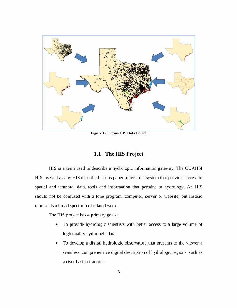
HIS is a t
as well as an
al and temp
ld not be co
esents a broa
The HIS p
• To
hi
• To
se
a r
term used to
ny HIS desc
poral data, t
onfused with
d spectrum o
project has 4
o provide hy
gh quality h
o develop a
eamless, com
river basin o
Figure 1-1 T
1.1 Th
o describe a
cribed in this
tools and in
h a lone pro
of related wo
4 primary go
ydrologic sc
ydrologic da
digital hydr
mprehensive
or aquifer
3
Texas HIS Dat
he HIS Pro
a hydrologic
s paper, refe
nformation t
ogram, comp
ork.
oals:
cientists with
ata
rologic obse
digital descr
ta Portal
oject
information
rs to a syste
that pertains
puter, server
h better acc
ervatory that
ription of hy
n gateway. T
m that provi
s to hydrolo
r or website
ess to a larg
t presents to
ydrologic reg
The CUAHS
ides access t
ogy. An HI
e, but instea
ge volume o
the viewer
gions, such a
SI
to
IS
ad
of
a
as
4
• To advance hydrologic science by enabling deeper insights into the
functioning of hydrologic processes and environments
• To enhance hydrologic education by bringing the digital hydrologic
observatory into the classroom.(Maidment, 2008))
The greatest challenge in accomplishing these initiatives is creating a system that
facilitates data exchange from both a data user and data provider’s perspective. From the
National Research Council’s 1991 report on “Opportunities in the Hydrologic Sciences”,
“Advances in hydrologic sciences depend on how well investigators can integrate
reliable, large scale, long term data sets.”(National Research Council, 1991) With large
datasets being a key to success, initial effort was placed in including major data providers
within the HIS.
1.2 Building an HIS
At the center of an HIS are data services. These services are built off web
services, software that enables computer to computer communication through the web.
This allows a data set to be published for online applications to read and access. In
attempting to integrate large scale, long term reliable data sets for the nation, CUAHSI
has compiled the largest collection of hydrologic metadata ever available from one
location through the publication of multiple data services. This list was a compilation of
both national scale and academic data sets (Maidment, 2008) and can be found in
Appendix A.
5
In total, the metadata of 1.7 million sites and 342 million data values were loaded
into a metadata catalog that allow for data exploration. The details of this process are
described in detail in later chapters.
1.3 Building a State HIS
The goal of this thesis is to provide insight into the development of a regional and
statewide HIS based on the continued development of a Texas HIS by the Center for
Research in Water Resources (CRWR) at the University of Texas Austin. A benefit of
creating a Texas HIS is the inclusion of data sets that will target a smaller scale audience.
A national HIS may find little use in a dataset that covers a single river reach. However, a
smaller scale HIS will be able to host these local and regional datasets for state users. As
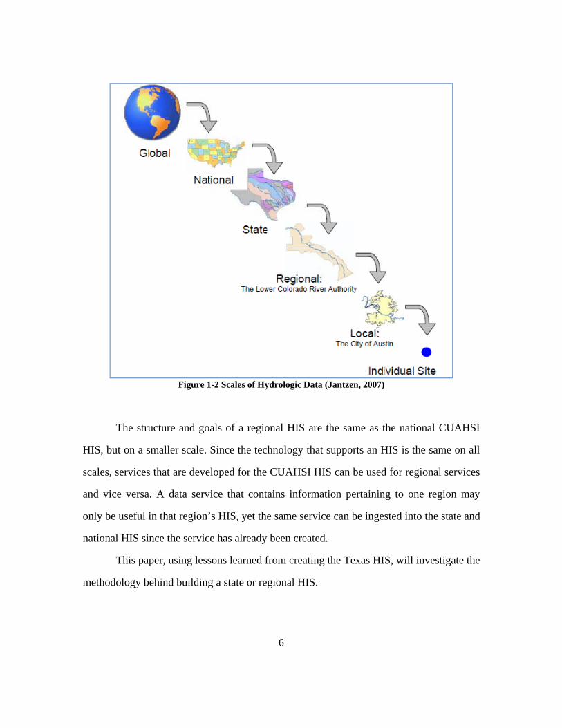
described in Tyler Jantzen’s 2007 thesis, there are multiple scales to hydrologic
information (Jantzen, 2007). In the same respect, there are multiple scales to an HIS. A
global HIS would need to be composed of global data services as well a compilation of
smaller national HIS’s. This is true for an HIS of any scale down to the smallest level.
(Figure 1-2)
6
Figure 1-2 Scales of Hydrologic Data (Jantzen, 2007)
The structure and goals of a regional HIS are the same as the national CUAHSI
HIS, but on a smaller scale. Since the technology that supports an HIS is the same on all
scales, services that are developed for the CUAHSI HIS can be used for regional services
and vice versa. A data service that contains information pertaining to one region may
only be useful in that region’s HIS, yet the same service can be ingested into the state and
national HIS since the service has already been created.
This paper, using lessons learned from creating the Texas HIS, will investigate the
methodology behind building a state or regional HIS.
7
1.4 Thesis Objectives
This Thesis addresses the following questions:
• What technologies are currently being utilized in creating a Texas HIS?
• What are the greatest difficulties in creating a Texas HIS and how can these be
overcome?
• What are the different roles played in a Texas HIS compared to a national HIS?
• What lessons have been learned in the data loading process?
• What future research is needed?

8
2 LITERATURE REVIEW
The building of a regional HIS requires the use of multiple technologies and the
coordination between multiple parties, from those involved with data management, data
collection to data access. Most of the technology that has been used to successfully
establish an HIS is mentioned within the Methodology chapter of this paper, however this
literature review takes a slightly broader look at this technology and other agencies who
have attempted to build similar systems to the HIS.
2.1.1 HYDROINFORMATICS
Defined by Kumar et al. 2006, the study of hydroinformatics is as follows:
“Hydroinformatics encompasses the development of theories, methodologies, algorithms and tools; methods for the testing of concepts, analysis and verification; and knowledge representation and their communication, as they relate to the effective use of data for the characterization of the water cycle through the various systems.”
The HIS project is an ongoing experiment in the field of hydroinformatics that
focuses around data communication. Any interested on the workings of an HIS should
consult Kumar el al, 2006 to gather a broad understanding of the technical workings
behind HIS technologies.
2.2 Similar HIS Efforts
Like any new technology, similar versions of the CUAHSI HIS are being
deployed across the country to promote scientific data use and exploration. Systems
typically combine a data management structure that interacts with a user query interface.
9
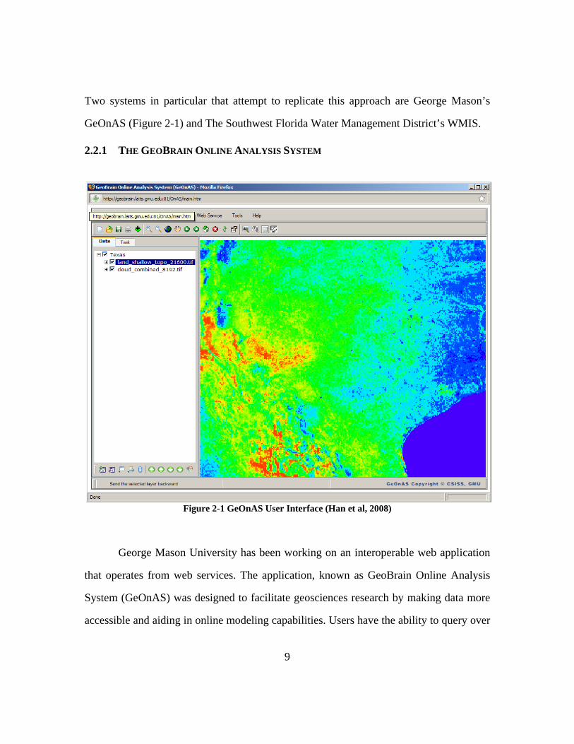
Two systems in particular that attempt to replicate this approach are George Mason’s
GeOnAS (Figure 2-1) and The Southwest Florida Water Management District’s WMIS.
2.2.1 THE GEOBRAIN ONLINE ANALYSIS SYSTEM
Figure 2-1 GeOnAS User Interface (Han et al, 2008)
George Mason University has been working on an interoperable web application
that operates from web services. The application, known as GeoBrain Online Analysis
System (GeOnAS) was designed to facilitate geosciences research by making data more
accessible and aiding in online modeling capabilities. Users have the ability to query over

10
200 geospatial data sets and perform several different analyses on the information. (Han
et al, 2008)
The GeOnAS system architecture is very similar to that of the Texas HIS. Data
sets are made accessible and metadata from these services are registered within a
Catalogue Services for Web (CSW), essentially a collection of available services. The
interface layer, (Figure 2-2) interacts with the web services based on user inputs.
Figure 2-2 GeOnAS Architecture (Center for Spatial Information Science and System)
The entire GeOnAS system essentially acts as a web application substitute for a
mapping tool, such as ESRI’s ArcMap, that is able to access web coverage services
(WCS), web mapping services (WMS), web feature services (WFS) and CSWs. Though
not built around hosting observation time series data, such as an HIS, the GeOnAS
provides insight into building a web based application that can harness web services.

11
2.2.2 WATER MANAGEMENT INFORMATION SYSTEM
Citing needs for a better organized data management system and improved
availability to the public, The Southwest Florida Water Management District decided to
reevaluate their data management practices. New data management groups were created
to find a better management system. The solution that came from this problem was the
implementation of the Water Management Information System (WMIS).
Using Oracle Warehouse Builder multiple data sets were fed into a data
warehouse that was able to be accessed by the WMIS. The system, specially designed for
facilitating permitting as well as exploring data, was designed by a diverse committee of
those involved with geospatial, hydrologic, water quality, hydrogeologic and regulatory
data.
Starting with a query tool, a user can investigate different metadata such as
location and variable to search for data (Figure 2-3).

12
Figure 2-3 WMIS User Search Interface
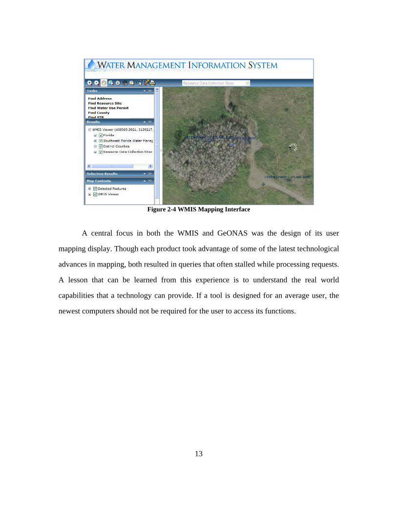
Data chosen to be displayed brings up a dynamic mapping interface in which a
user can visually examine sites of interest (Figure 2-4). These sites can then be saved and
brought back into the user search interface where more information about the site can be
found and downloaded. (Dicks, Nov. 2008)
13
Figure 2-4 WMIS Mapping Interface
A central focus in both the WMIS and GeONAS was the design of its user
mapping display. Though each product took advantage of some of the latest technological
advances in mapping, both resulted in queries that often stalled while processing requests.
A lesson that can be learned from this experience is to understand the real world
capabilities that a technology can provide. If a tool is designed for an average user, the
newest computers should not be required for the user to access its functions.
14
3 METHODOLOGY
3.1 The HIS Model
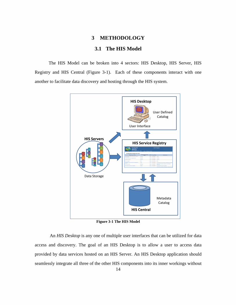
The HIS Model can be broken into 4 sectors: HIS Desktop, HIS Server, HIS
Registry and HIS Central (Figure 3-1). Each of these components interact with one
another to facilitate data discovery and hosting through the HIS system.
Figure 3-1 The HIS Model
An HIS Desktop is any one of multiple user interfaces that can be utilized for data
access and discovery. The goal of an HIS Desktop is to allow a user to access data
provided by data services hosted on an HIS Server. An HIS Desktop application should
seamlessly integrate all three of the other HIS components into its inner workings without
HIS Servers
Data Storage
HIS Service Registry
HIS Central
HIS Desktop
User Interface
MetadataCatalog
User Defined Catalog

15
the user having to know how they work. Less elaborate HIS Desktops may require some
outside exploration by the user to find the source of data that is desired.
The HIS Registry allows a user or web service to explore what types of data
services exist on registered HIS Servers. A registry is especially beneficial when it can
provide an interface that facilitates the exploration of HIS Central, a comprehensive
metadata storage database of all registered water data services. It is the central component
in which data suppliers can list their web services to make them available for users to
access. This component of the HIS model allows users to query metadata from all the
data services that are provided in an HIS Central. Every descriptive aspect of a data
service, such as site, variable and method are housed within one central database in order
to support user and web service queries. The HIS Central, also should contain a Master
Series Catalog for use in metadata queries. A series catalog contains an individual row
for each sampling of a variable. A dataset that measures four variables at five different
locations would have a series catalog with 20 total rows, one for each variable at each
location. Each unique method and offset also results in another row in a series catalog.
The master catalog is the synthesis of each registered data service’s series catalog.
The fourth component of the HIS Model is the HIS Server. An HIS Server is any
server that hosts data services or other HIS applications. There are no specifications to
the size of an HIS Server, it can host any amount of data services and is connected to the
HIS by registering its services within the HIS Registry. An HIS Server can be housed by
any number of organizations depending on the needs of the data provider. For instance, in
cases when a database is constantly updated, such as instantaneous data, it may be more
appropriate to host that database on the data collection organization’s server. However, in
the case of a static database, no longer modified by an agency, a larger HIS Server may
16
be better suited to host the data service. The following methodology will discuss the
process of creating a generic HIS and how the HIS model is involved in each stage.
3.2 Data Housing
3.2.1 THE OBSERVATIONS DATA MODEL
A major issue that needs to be overcome prior to collecting and distributing data
through an HIS is the integration of multiple data formats. Collecting data from multiple
sources results in different data types, formats and content. Without sharing a common
format, it is difficult for any application to make sense of databases that house very
different information and come from a variety of sources. A solution to having sources
conform to one format is finding a common link between them. The Observations Data
Model (ODM), developed by Jeff Horsburgh and David Tarboton of Utah State
University, can act as this common thread. For this reason the ODM is essential to an HIS
Server. It provides an effective method of housing each separate data service. The ODM
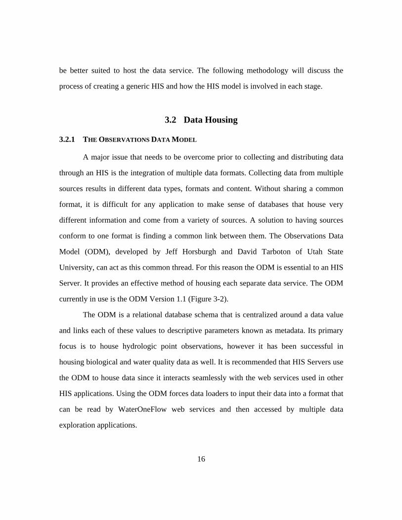
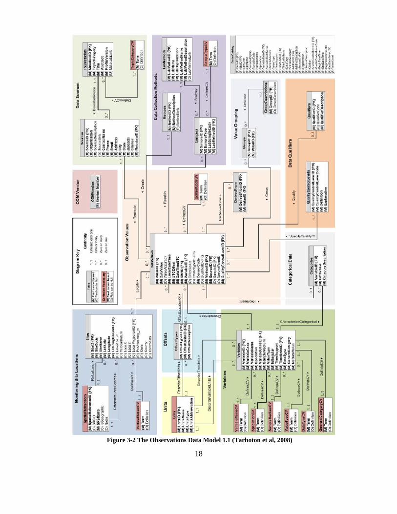
currently in use is the ODM Version 1.1 (Figure 3-2).
The ODM is a relational database schema that is centralized around a data value
and links each of these values to descriptive parameters known as metadata. Its primary
focus is to house hydrologic point observations, however it has been successful in
housing biological and water quality data as well. It is recommended that HIS Servers use
the ODM to house data since it interacts seamlessly with the web services used in other
HIS applications. Using the ODM forces data loaders to input their data into a format that
can be read by WaterOneFlow web services and then accessed by multiple data
exploration applications.
17
With various formatting and vocabularies being used by different sources, a
program may not recognize uncommon or abbreviated terms used to describe data.
However, by inserting this data into the ODM, the need to recognize a term is erased.
Instead the WaterOneFlow web services grab information based on its location within
each table. Even though the language does not understand what a term such as Dissolved
Oxygen represents, it understands it is a variable name given its location in the ODM.
Though naming conventions, locations and collection methods may vary, by
utilizing the ODM, these differences can be overlooked when accessing data so two data
sets, initially in different formats, can be accessed by using one retrieval method.
18
Figure 3-2 The Observations Data Model 1.1 (Tarboton et al, 2008)

19
3.2.2 THE OBSERVATIONS DATA MODEL STRUCTURE
The ODM, as mentioned above, is a relational database that is centered on data
values. Each data value is linked to a timestamp as well as multiple descriptive metadata
tables that provide information about that specific data point. These tables, provided in
Table 3-1, encourage data loaders to provide an array of descriptive information about
each service.
Table 3-1 Primary ODM Tables
Primary Table Names Table Fields Mandatory Primary Table Names Table Fields MandatoryValueID Yes SiteID Yes
DataValue Yes SiteCode YesValueAccuracy SiteName YesLocalDateTime Yes Latitude YesUTCOffset Yes Longitude Yes
DateTimeUTC Yes LatlongDatumID YesSiteID Yes Elevation_m
VariableID Yes VerticalDatumOffsetValue LocalXOffsetTypeID LocalYCensorCode Yes LocalProjectionIDQualifierID PosAccuracy_mMethodID Yes StateSourceID Yes CountySampleID Comments
DerivedFromID MethodID YesQualityControlLevelID Yes MethodDescription Yes
MethodLinkVariableID Yes SourceID Yes
VariableCode Yes Organization YesVariableName Yes SourceDescription YesSpeciation Yes SourceLink
VariableUnitsID Yes ContactName YesSampleMedium Yes Phone Yes
ValueType Yes Email YesIsRegular Yes Address Yes
TimeSupport Yes City YesTimeUnitsID Yes State YesDataType Yes ZipCode Yes
GeneralCategory Yes Citation YesNoDataValue Yes MetadataID Yes
Variables
Sites
Methods
Sources
DataValues

20
Though only the primary tables are listed above, in total there are 27 different
tables that are linked to each individual data value. The ODM uses numerical ID’s or
keys to link one table to another. Figure 3-3 demonstrates the ODM table in a simplified
form to expound on the linking mechanisms of the schema. In the DataValue Table
SiteID and VariableID are considered foreign keys since they link that table to another.
Within the Variables Table and Sites Table, the VariableID and SiteID, respectively, are
considered the primary key since they link all the fields in that table to another. Figure
3-3 demonstrates that each VariableID links a data value to a single variable in the
Variable Table. Within the Variable Table, further links are made to link each variable
with appropriate units. This methodology is used in each of the ODM’s tables.
Figure 3-3 Simplified ODM Representation
21
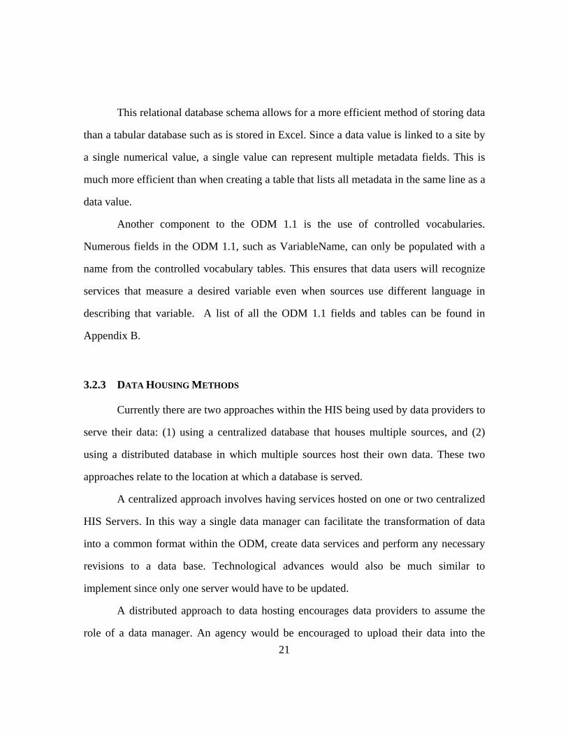
This relational database schema allows for a more efficient method of storing data
than a tabular database such as is stored in Excel. Since a data value is linked to a site by
a single numerical value, a single value can represent multiple metadata fields. This is
much more efficient than when creating a table that lists all metadata in the same line as a
data value.
Another component to the ODM 1.1 is the use of controlled vocabularies.
Numerous fields in the ODM 1.1, such as VariableName, can only be populated with a
name from the controlled vocabulary tables. This ensures that data users will recognize
services that measure a desired variable even when sources use different language in
describing that variable. A list of all the ODM 1.1 fields and tables can be found in
Appendix B.
3.2.3 DATA HOUSING METHODS
Currently there are two approaches within the HIS being used by data providers to
serve their data: (1) using a centralized database that houses multiple sources, and (2)
using a distributed database in which multiple sources host their own data. These two
approaches relate to the location at which a database is served.
A centralized approach involves having services hosted on one or two centralized
HIS Servers. In this way a single data manager can facilitate the transformation of data
into a common format within the ODM, create data services and perform any necessary
revisions to a data base. Technological advances would also be much similar to
implement since only one server would have to be updated.
A distributed approach to data hosting encourages data providers to assume the
role of a data manager. An agency would be encouraged to upload their data into the

22
ODM, create data services and host their own HIS Server. The advantage to this
distributed approach lies in the data provider’s familiarity with the data and diminishing
the need to transport data between agencies. Data services loaded through a centralized or
distributed HIS would have no effect in how users are able to access data since all data
services are registered individually within an HIS Registry.
Figure 3-4 Centralized vs. Distributed System
A third option is the combination of the two methods. Since some agencies are
more likely to have the facilities and desire to host data than others, it is likely that some
HIS Servers will host multiple data services from multiple sources while others may only
chose to host a single data service. No matter where an ODM is located it is linked to the
overall HIS by the use of web services.
3.2.4 HYBRID WEB SERVICES
Another method of hosting a data service is through the procedure of hosting a
hybrid service. This involves hosting only select attributes through the ODM and
scrapping other information off a remote service. The Texas Coastal Ocean Observation
Network (TCOON) database was the first hosted in this way. TCOON metadata was
accessed through a download of an XML file and loaded into an ODM database. The
23
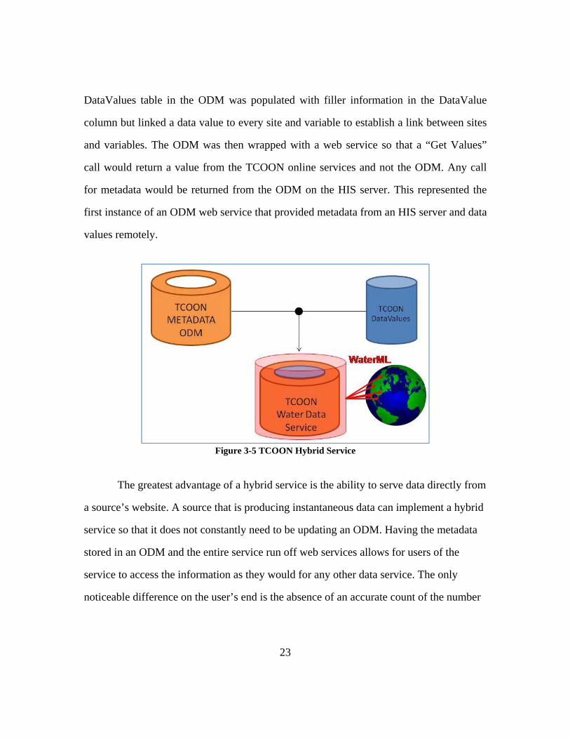
DataValues table in the ODM was populated with filler information in the DataValue
column but linked a data value to every site and variable to establish a link between sites
and variables. The ODM was then wrapped with a web service so that a “Get Values”
call would return a value from the TCOON online services and not the ODM. Any call
for metadata would be returned from the ODM on the HIS server. This represented the
first instance of an ODM web service that provided metadata from an HIS server and data
values remotely.
Figure 3-5 TCOON Hybrid Service
The greatest advantage of a hybrid service is the ability to serve data directly from
a source’s website. A source that is producing instantaneous data can implement a hybrid
service so that it does not constantly need to be updating an ODM. Having the metadata
stored in an ODM and the entire service run off web services allows for users of the
service to access the information as they would for any other data service. The only
noticeable difference on the user’s end is the absence of an accurate count of the number
24
of data values in the service due to the continuously growing number of data values
recorded.
3.3 Data Upload
3.3.1 SQL SERVER INTEGRATED SERVICES DATA LOADING
SQL Server Integrated Services (SSIS) is a Microsoft product developed to aide
in data management in conjunction with SQL Server, Microsoft’s data platform. Though
it has multiple features, for the specific data loading process that is required by the ODM,
the data scripts tool prove to be most beneficial for transformation of the data into ODM
data types and format requirements. These data type requirements can be found in
Appendix B.
Every data set requires a unique loading process depending on the original
formatting and organization of data. For this reason it is difficult for a single
methodology to be produced that can be applied to a specific data set. Using SSIS
typically involves the implementation of a four step process: pre-formatting, data
ingestion into SSIS, data transformation with SSIS scripts and data upload into the ODM.
Pre-formatting involves readying the data for consumption by SSIS. This step can
be passed over if the data is in a format that is easily digestible by SSIS or if the data
loader would rather write a more involved script. Alterations can be as simple as
combining multiple data files into a single comprehensive file for SSIS to access.
Another example may be the reformatting of a date format within a more user friendly
data manipulation program such as Microsoft Excel. Though this can be performed
through a SSIS script, a user less comfortable using the Visual Basic scripting language,

25
required by SSIS scripts, may prefer to avoid scripting. In the SSIS loading method
described in Appendix C, each ODM table is loaded separately into the ODM
Data ingestion with SSIS can be a simple process, so long as the data to be
ingested is well organized. Complex data sets are prone to slight errors in formatting
which can propagate into larger errors when attempting to upload the data into SSIS. This
is especially prevalent with a fixed width data format, where a misplaced divider can
truncate data columns incorrectly. Though not required, ideally data should be comma
delimited before attempting to process it with SSIS to facilitate the data upload process.
Once the connection is made between SSIS and the data set to be uploaded a
unique script has to be written that translates the original data format and organization to
fit within the ODM. Scripts are unique to not only to each data set but to each table of
data that is being uploaded; a Sites script is different than a Data Values script. The tables
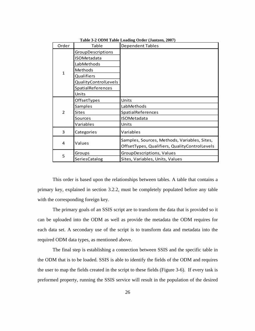
must be uploaded according to priorities set by the ODM as displayed in Table 3-2.
26
Table 3-2 ODM Table Loading Order (Jantzen, 2007) Order Table Dependent Tables
GroupDescriptionsISOMetadataLabMethodsMethodsQualifiersQualityControlLevelsSpatialReferencesUnitsOffsetTypes UnitsSamples LabMethodsSites SpatialReferencesSources ISOMetadataVariables Units
3 Categories Variables
4 ValuesSamples, Sources, Methods, Variables, Sites, OffsetTypes, Qualifiers, QualityControlLevels
Groups GroupDescriptions, ValuesSeriesCatalog Sites, Variables, Units, Values
5
2
1
This order is based upon the relationships between tables. A table that contains a
primary key, explained in section 3.2.2, must be completely populated before any table
with the corresponding foreign key.
The primary goals of an SSIS script are to transform the data that is provided so it
can be uploaded into the ODM as well as provide the metadata the ODM requires for
each data set. A secondary use of the script is to transform data and metadata into the
required ODM data types, as mentioned above.
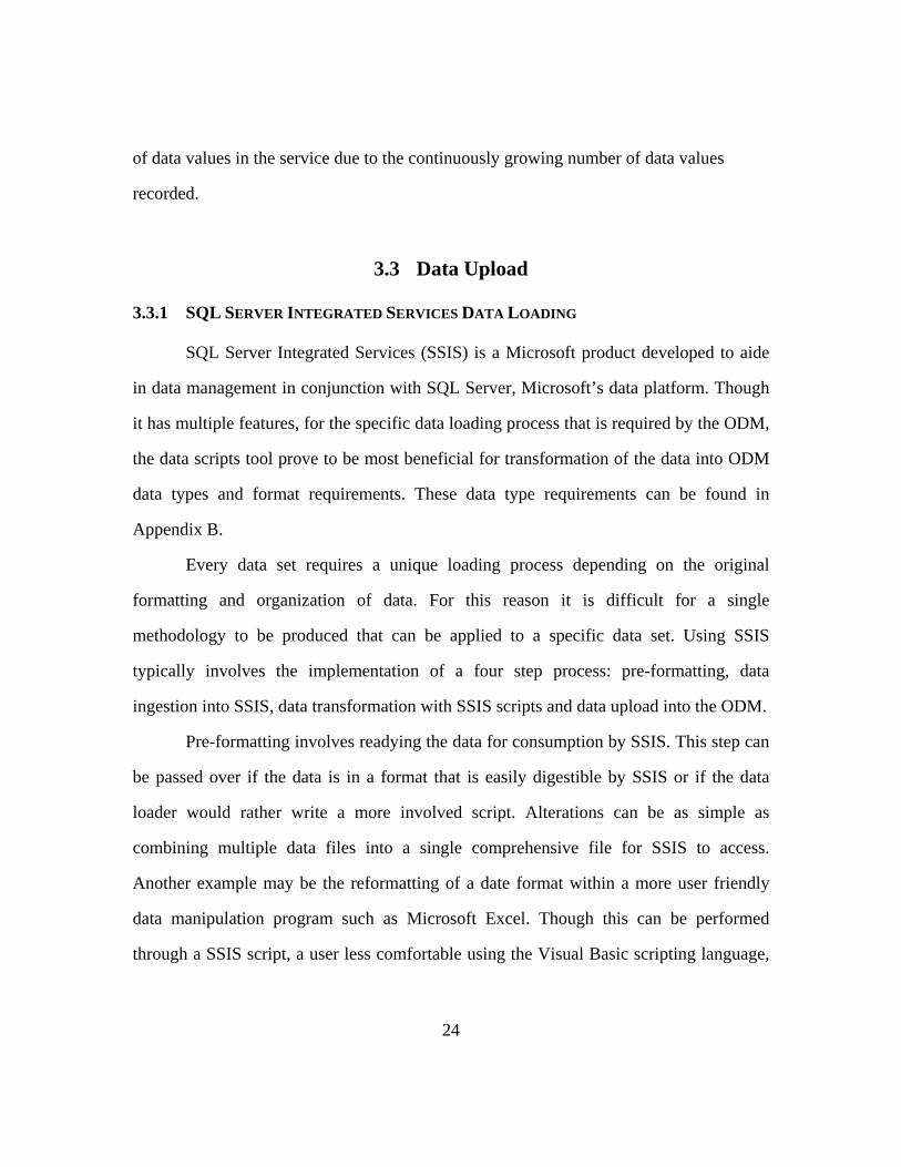
The final step is establishing a connection between SSIS and the specific table in
the ODM that is to be loaded. SSIS is able to identify the fields of the ODM and requires
the user to map the fields created in the script to these fields (Figure 3-6). If every task is
preformed property, running the SSIS service will result in the population of the desired
27
ODM table. Multiple tables can be loaded in succession as long as the order fits to the
ODM order mentioned earlier.
Figure 3-6 SSIS Field Mapping
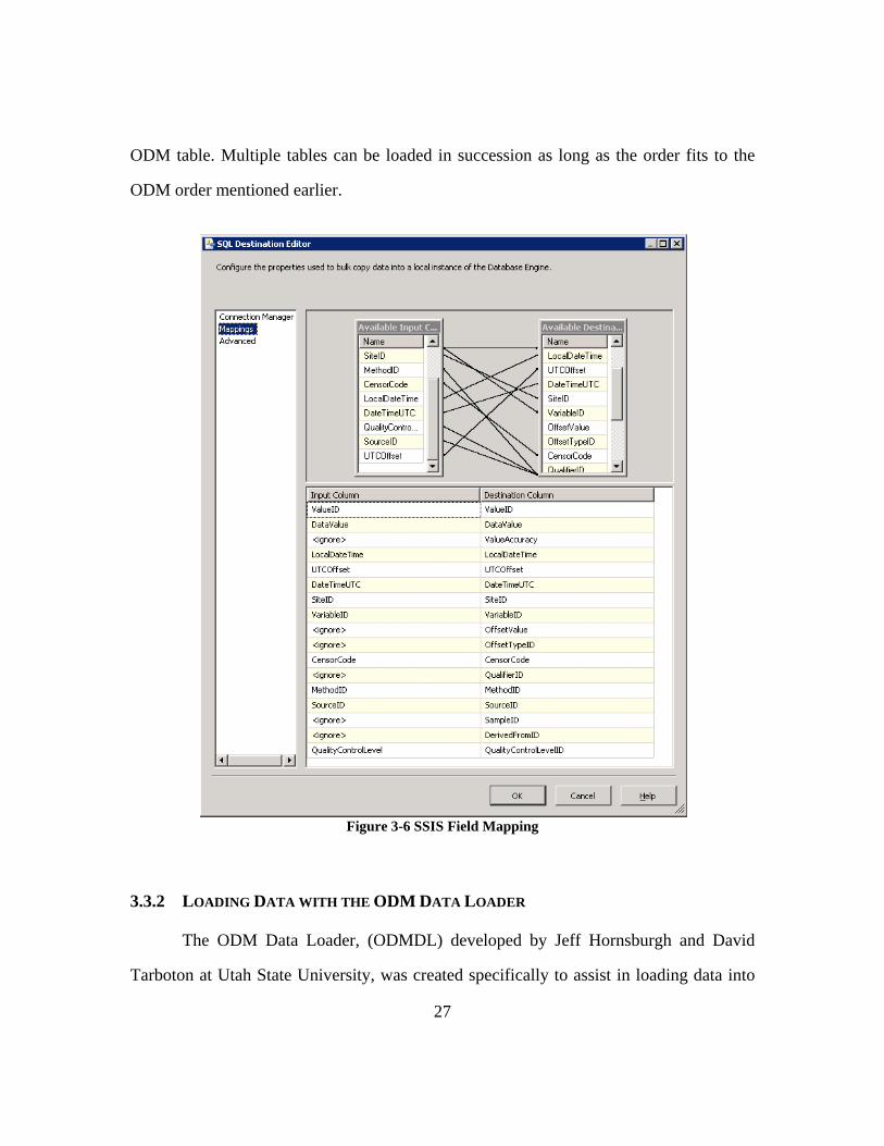
3.3.2 LOADING DATA WITH THE ODM DATA LOADER
The ODM Data Loader, (ODMDL) developed by Jeff Hornsburgh and David
Tarboton at Utah State University, was created specifically to assist in loading data into

28
the ODM. Available for download on the CUAHSI website (www.his.cuahsi.org), this
program is more user friendly than SSIS and does not require a user to be familiar with a
programming language. The ODMDL has the ability to read files in the comma delimited
(.csv) and Microsoft Excel 2003(.xls) formats, thus enabling data managers to use a
program such as Excel to perform necessary transformations. Where, in the previous
section, SSIS scripts were used to add required metadata, the ODMDL requires the user
to submit data conforming to formatting outlined in the ODMDL specifications. The
ODMDL then is able to recognize the column names in each data file and associate them
with a field name in the ODM. The ODMDL recognizes field headings such as
“SiteCode” and “Sitename” as field titles within the ODM Sites table (Figure 3-7 ODM
Data Loader 1.1) and is able to load each column into the proper place within the ODM
based on this heading. At the bottom of the loader the phrase ‘You are loading Sites”,
displays to the user that the program has correctly identified what is to be loaded into the
ODM.
29
Figure 3-7 ODM Data Loader 1.1
Unlike the SSIS described method, the ODMDL can perform bulk data loads of
all the ODM fields at once as well as load individual tables at a time. This allows the user
more flexibility in how to organize data before uploading it into the ODM. (Horsburgh,
2008)
3.3.3 COMPARISON OF THE ODMDL AND SSIS DATA LOADING METHODS
Both of these methods can be used successfully on any database. However, one
method may be preferable to another based on the complexity or size of the database.
Since SSIS does not always require data to be transformed before loading, databases that
may be distributed in multiple data files are able to be accessed without compiling the
data into one large database or having multiple data loads. SSIS is able to handle loading
30
extremely large data sets better than the ODMDL because of quality control aspects built
into the ODMDL. This quality control setting ensures that no two lines of data loaded
into the ODM are identical across all fields. Though this is beneficial in ensuring a
minimum quality of data, it does have negative effects on the program’s efficiency to
load data.
Smaller data sets that require fewer transformations typically can be loaded in a
much quicker and simpler manner by using the ODMDL. This method, especially to
those unfamiliar with programming, is much more straightforward and should be the
method pursued by most data managers. To become familiar with the SSIS loading
process takes practice as well as programming knowledge and should be used primarily
by those loading multiple data sets, and not by one time data loaders.
If beneficial, a user can use both methods as well as manually imputing metadata
into the ODM. Manually imputing metadata into the ODM is useful when very little data
is needed to be added to an ODM table. An example of this would be filling out the
Methods table with a single method description. In this case it would be more efficient to
edit the ODM directly instead of relying on a program to assist in the data upload
process.
Manually editing the ODM is a simple process of accessing the ODM within SQL
Server Management Studios and pulling up a desired table. Any cell, no matter if it is
already populated or empty, may be editing by just clicking on the cell. For a new row of
data to be entered into a table, all necessary fields (Table 3-1) must be populated and the
correct links must be in place.
Using all three methods may be useful if a large data set is to be uploaded with
relatively small amounts of site and/or variable metadata. In this case, the sites and
variable ODM tables can be populated by using the ODMDL while the large amount of

31
data values can be uploaded by SSIS. Essentially there is no one right way to load data
and it is up to the data manager to decide which method is most useful in each unique
case.
3.4 Data Publication
Data publication is the act of making data readily available for potential users to
access. This procedure is a two step process; the first is allowing access to the data, the
second is registering the data service. Within the HIS the first step is achieved through
the use of WaterOneFlow web services. The second step requires the implementation of
an HIS Registry to allow data managers to advertise what services are available.
3.4.1 WATERONEFLOW SERVICES AND THE ODM
WaterOneFlow services are the group of web services created by CUAHSI
(Zaslavsky, Valentine, & Whiteaker, 2007) to be used with hydrologic data. These web
services were designed to use a variation of the Extensible Markup Language (XML)
called the Water Markup Language (WaterML) to interact with the ODM. This language
requests data by retrieving tagged lines of code. WaterOneFlow uses the calls
“GetVariableInfo”, “GetSites”, “GetSiteInfo” and “GetValues” to allow applications to
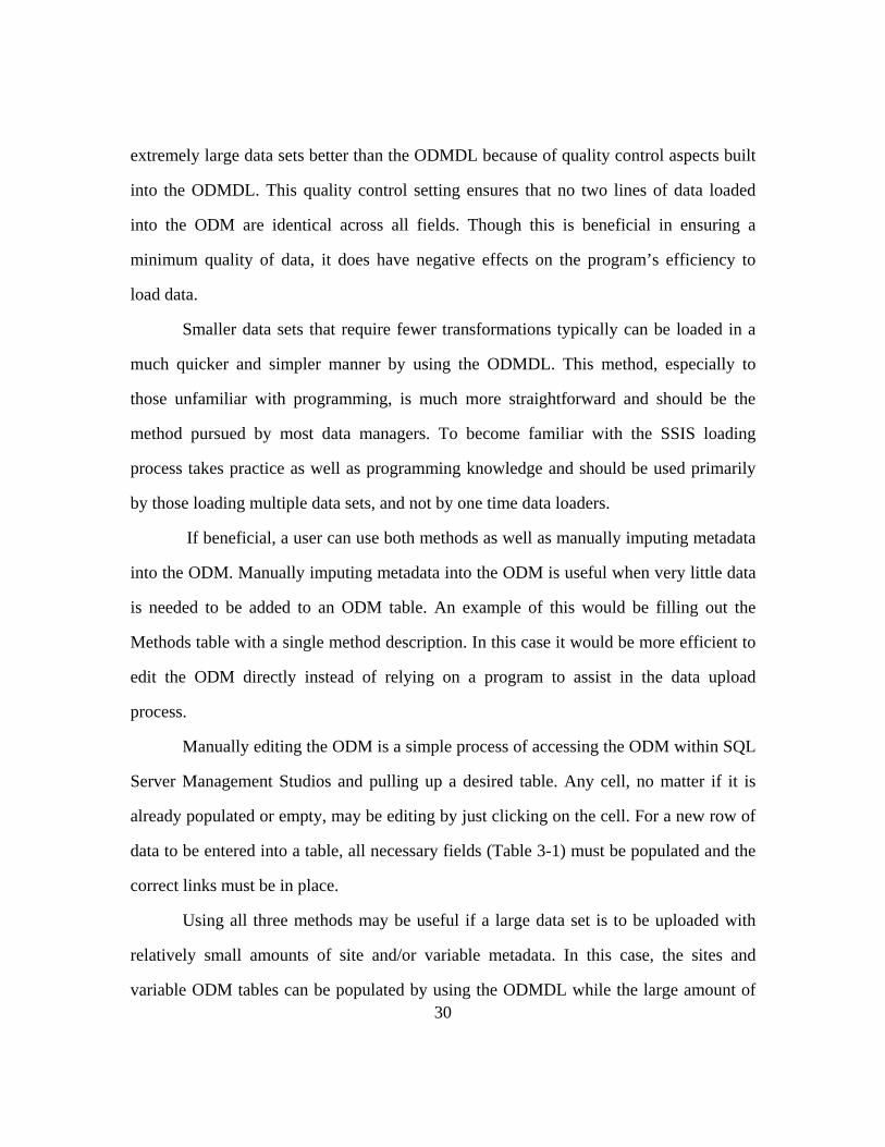
return desired data and metadata from a service. Figure 3-8 displays a return from a
“GetVariable Info” call performed when accessing a web service.
32
Figure 3-8 Water Markup Language
These calls all return specific information from the ODM. The “GetVariables”
call returns metadata about the variables that are measured within the ODM. ‘GetSites”
returns a list of every site within the ODM as well as their metadata information.
“GetSitesInfo” returns what variables are recorded at a specific site and “GetValues”
returns data values given a start and end date, site and variable.
The ODM 1.1 is able to wrap fields in WaterML code so it can be retrieved when
a call is made. This called returned all the variable metadata for a variable named “Gage
Height”. Between start “<variable>” tag and end “</variable>” tag, is housed all the
variable metadata contained in the ODM that describes a specific variable. In calling for
the variable information, a request returns applicable variable metadata. Each of the calls
performed return specific data in this same method.
3.4.2 WATERONEFLOW AND WEB SERVICE DEFINITION LANGUAGE
The creation of a Web Service Definition Language (WSDL) addresses is the
central component of sharing ODM data. A WSDL address is the equivalent to a data
window; once accessed an application is told where to find a web service and the type of
33
language it is using to communicate, in this case WaterML (Alameda, 2006). Each data
service has its own unique WSDL that allows the data service to communicate outside its
server. Once a WSDL is utilized, an application can send a request that interacts with the
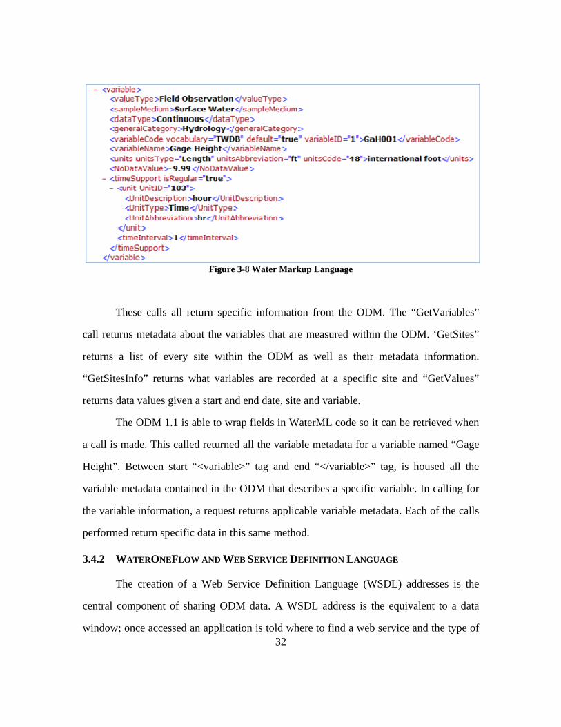
WaterOneFlow web services that are provide access to a database (Figure 3-9). An
application may send out a request, such as “Get Sites” through to the WSDL address and
web services will return site metadata from the service. Provided with a WSDL address a
user does not need to be aware of the technical working of a web services to access their
utility. With the push of a button, services work behind the scene to retrieve requested
information.
Figure 3-9 WSDL Data Request
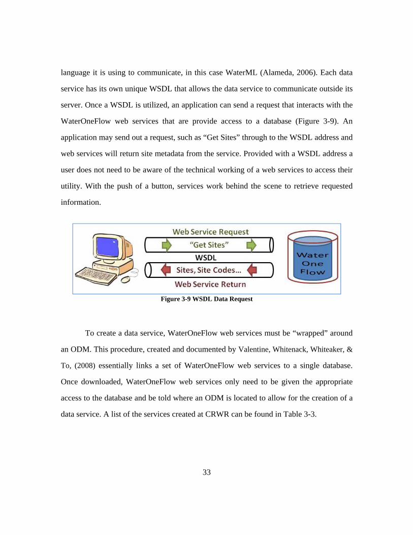
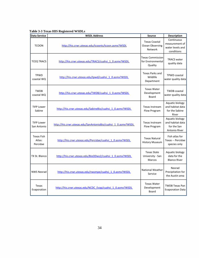
To create a data service, WaterOneFlow web services must be “wrapped” around
an ODM. This procedure, created and documented by Valentine, Whitenack, Whiteaker, &
To, (2008) essentially links a set of WaterOneFlow web services to a single database.
Once downloaded, WaterOneFlow web services only need to be given the appropriate
access to the database and be told where an ODM is located to allow for the creation of a
data service. A list of the services created at CRWR can be found in Table 3-3.
34
Table 3-3 Texas HIS Registered WSDLs
Data Service WSDL Address Source Description
TCOON http://his.crwr.utexas.edu/tcoonts/tcoon.asmx?WSDLTexas Coastal
Ocean Observing Network
Continuous measurement of water levels and
conditions
TCEQ TRACS http://his.crwr.utexas.edu/TRACS/cuahsi_1_0.asmx?WSDL Texas Commission for Environmental
Quality
TRACS water quality data
TPWD coastal WQ
http://his.crwr.utexas.edu/tpwd/cuahsi_1_0.asmx?WSDL Texas Parks and
Wildlife Department
TPWD coastal water quality data
TWDB coastal WQ
http://his.crwr.utexas.edu/TWDB/cuahsi_1_0.asmx?WSDL Texas Water Development
Board
TWDB coastal water quality data
TIFP Lower Sabine
http://his.crwr.utexas.edu/SabineBio/cuahsi_1_0.asmx?WSDL Texas Instream Flow Program
Aquatic biology and habitat data for the Sabine
River
TIFP Lower San Antonio
http://his.crwr.utexas.edu/SanAntonioBio/cuahsi_1_0.asmx?WSDL Texas Instream Flow Program
Aquatic biology and habitat data
for the San Antonio River
Texas Fish Atlas:
Percidae http://his.crwr.utexas.edu/Percidae/cuahsi_1_0.asmx?WSDL
Texas Natural History Museum
Fish atlas for Texas ‐‐ Percidae species only
TX St. Blanco http://his.crwr.utexas.edu/BioODws2/cuahsi_1_0.asmx?WSDL Texas State
University ‐ San Marcos
Aquatic biology data for the Blanco River
NWS Nexrad http://his.crwr.utexas.edu/nwsmpe/cuahsi_1_0.asmx?WSDL National Weather
Service
Nexrad Precipitation for the Austin area
Texas Evaporation
http://his.crwr.utexas.edu/NCDC_Evap/cuahsi_1_0.asmx?WSDL Texas Water Development
Board
TWDB Texas Pan Evaporation Data
35
3.4.3 WEB MAPPING SERVICES
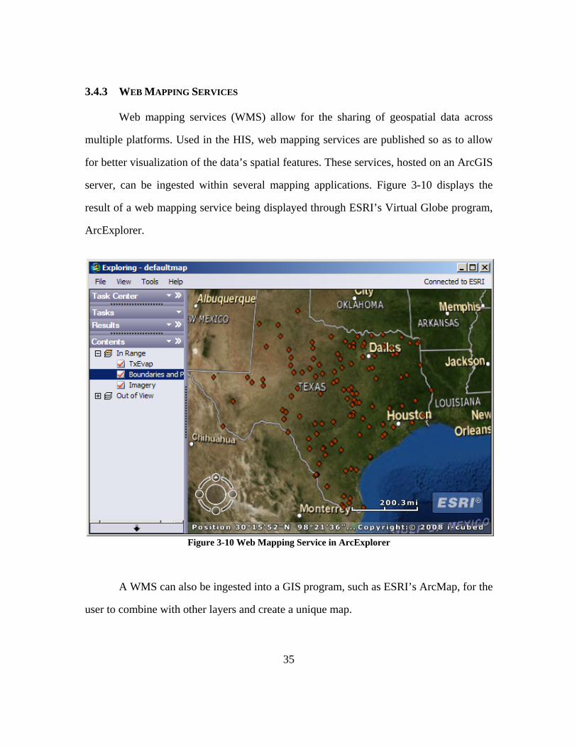
Web mapping services (WMS) allow for the sharing of geospatial data across
multiple platforms. Used in the HIS, web mapping services are published so as to allow
for better visualization of the data’s spatial features. These services, hosted on an ArcGIS
server, can be ingested within several mapping applications. Figure 3-10 displays the
result of a web mapping service being displayed through ESRI’s Virtual Globe program,
ArcExplorer.
Figure 3-10 Web Mapping Service in ArcExplorer
A WMS can also be ingested into a GIS program, such as ESRI’s ArcMap, for the
user to combine with other layers and create a unique map.

36
The mapping services hosted at CRWR were created by using ESRI’s ArcServer
applications. Construction of a WMS is as simple as creating a map, allowing ArcServer
to access it and selecting the map to be hosted as a WMS. A URL is created that allows
access to the WMS. The drawback of this service is that it lacks any attributes that the
original feature class once contained. A WMS simply provides a visual display of
metadata and does not contain the original data or metadata.
3.4.4 WEB FEATURE SERVICES
While a WMS service allows for the sharing of geospatial displays, a web feature
service (WFS) provides a method of sharing data stored within a geodatabase. Using a
similar procedure to creating a WMS, to build a WFS, a geodatabase with the feature
class to be shared should be brought onto an HIS Server. The geodatabase simply needs
to be selected to be hosted by ArcServer and a WFS URL is created that allows outside
access to the service. Once created, a user can ingest the service into ArcCatalog by
providing the WFS link. Connected to the service, a user can select multiple feature
classes to view and can export desired data onto a local machine.
3.4.5 WEB FEATURE AND WEB MAPPING SERVICES WITHIN THE HIS
Web feature and web mapping services, when used with WaterOneFlow web
services, provide a powerful tool for data sharing. The power behind both WFS and
WMS is their ability to share geospatial data. They are both useful tools in data
exploration but neither is effective in sharing temporal data. The ODM and
WaterOneFlow web services provide an excellent foundation for accessing time series
data, but do not facilitate the exploration of available data. Integrating these services then
allows for both spatial exploration and temporal access.

37
The merging of WaterOneFlow and Web Feature services involves creating a
feature class that allows a user to evaluate the contents of a data service. This feature
class must provide at very least a description of variables sampled, locations of samples
and a time frame of the samples. This table, first created as a way to access hydrology
data through ArcGIS, is a slight variation of a MySelect Table (Table 3-4). This table
includes the basic metadata information about every site and variable a service offers.
Table 3-4 MySelect Table Fields
Using this table, an HIS Catalog can be made of every site and variable available through
WaterOneFlow web services. This catalog, having a spatial component, can be displayed
on a map and then served as either a WMS or WFS. Including a WSDL field in this
catalog allows for a user to be able to access the time series data that a WFS or WMS
would not be able to provide. Thus the creation of a WaterOneFlow web service along
with a MySelect WFS and WMS connects services in time and space.
Field Heading ExampleWSDL http://his.crwr.utexas.edu/TWDB/cuahsi_1_0.asmx?WSDL
Network TWDBSiteCode D3394
VariableCode SAL001StartDate 10/23/84 8:15EndDate 5/13/98 15:34Latitude 28.9750Longitude ‐95.2667SiteName Swan Lake Boat BasinVarName SalinityUnits parts per thousand
NSiteCode TWDB:D3394NVarCode TWDB:SAL001
VarCode

38
3.4.6 DATA REGISTRY
A critical component to data publication is ensuring clients are aware of the
services that exist. A method for this is creating an HIS Registry of all services that are
available within an HIS. At the very least this should be a listing of what type of service
is available with a description of site locations, variables measured, dates of measurement
and a time span of the measurement period. Figure 3-11 displays a portion of the CRWR
Texas HIS Registry.
Figure 3-11 Data.Crwr Texas HIS Data Service Registry
Each line represents a different service that users can access to explore the
geographic extent of the data as well as a brief description of the service.
One benefit of an HIS Registry is the ability to create a comprehensive metadata
catalog, known as an HIS Central. A metadata catalog stores specific metadata fields
from registered services to allow users to later query what types of data is available.
39
Being able to base queries off this catalog allows users to bypass examining individual
services and instead treat the HIS as one unified data source.
This uniting of temporal and spatial data was performed in the Texas HIS to
create a Texas Salinity Catalog. Using a site catalog from three Texas HIS data sources,
Texas Water Development Board (TWDB), Texas Parks and Wildlife Department
(TPWD) and Texas Commission on Environmental Quality, the locations where salinity
was measured were copied to another table along with the information needed to populate
the MySelect table that housed all relevant site and variable information as well as
WSDL addresses where time series data could be accessed. The records from each
service were then brought together to produce a Texas Salinity Catalog. In total, over
7,800 sites recorded more than 330,000 data values measuring salinity concentration.
This Salinity Layer represents a thematic data layer; an organization of data under a
central theme (Figure 3-12 Salinity Thematic Layer).

40
Figure 3-12 Salinity Thematic Layer
The stride for thematic organization represents a progression of creating services
that are focused around metadata based queries over service based queries. A user
typically is not concerned with the source of the data that is being used; instead multiple
sources can be accessed to provide a greater quantity of information. These thematic
layers are considered secondary or derived services since they are created from metadata
of multiple data services. A sample from the Salinity Thematic Series table (Table 3-5)
can be seen below that contains sample metadata from several of the services included in
the Salinity Thematic Layer. Each listing is an example of salinity measurements being
taken at a unique site from one of several services that can all be accessed through a
WSDL included in that row.

41
Table 3-5 Salinity Thematic Series
3.5 Data Discovery
Data discovery includes all elements of data downloading, user queries and data
exploration. The central aspect of data discovery is the multiple applications that can
interact with web services. These applications should allow a user to explore what data is
available at different geographic locations as well as provide access to a service’s data
and metadata. Currently there are several applications that have capabilities to read the
web services discussed earlier, however this thesis will examine three most closely
related to the Texas and CUAHSI HIS projects; HydroSeek, HydroExcel and The TNRIS
Geospatial Emergency Management Support System (GEMSS) Viewer.
3.5.1 HYDROSEEK
The HydroSeek viewer was developed by Bora Boren and Michael Piasecki at
Drexel University. The viewer operates off of a HIS Central metadata catalog of several
services that allows for keyword queries of available services at Drexel. The HIS Central
was relocated at the San Diego Super Computer Center and is constantly being updated
with newly created services. (Beran, 2007).
Once a service is registered, metadata fields from the ODM are ingested into a
metadata catalog that holds the metadata for every registered service. After the metadata
WSDL SiteCode VarCode ValueCounthttp://his.crwr.utexas.edu/TWDB/cuahsi_1_0.asmx?WSDL TWDB:D1137 TWDB:SAL001 304http://his.crwr.utexas.edu/TPWD/cuahsi_1_0.asmx?WSDL TPWD:b2s247 TPWD:SAL001 19http://his.crwr.utexas.edu/TPWD/cuahsi_1_0.asmx?WSDL TPWD:b2s248 TPWD:SAL001 104http://ccbay.tamucc.edu/CCBayODWS/cuahsi_1_0.asmx?WSDL ODM:H1 ODM:SalinityGrab 270http://ccbay.tamucc.edu/CCBayODWS/cuahsi_1_0.asmx?WSDL ODM:H2 ODM:SalinityGrab 499http://his.crwr.utexas.edu/tcoonts/tcoon.asmx?WSDL TCOON:075 TCOON:sal 2http://his.crwr.utexas.edu/tcoonts/tcoon.asmx?WSDL TCOON:076 TCOON:sal 2http://his.crwr.utexas.edu/TRACS/cuahsi_1_0.asmx?WSDL TCEQ:10726 TCEQ:00480 3http://his.crwr.utexas.edu/TRACS/cuahsi_1_0.asmx?WSDL TCEQ:10727 TCEQ:00480 7
42
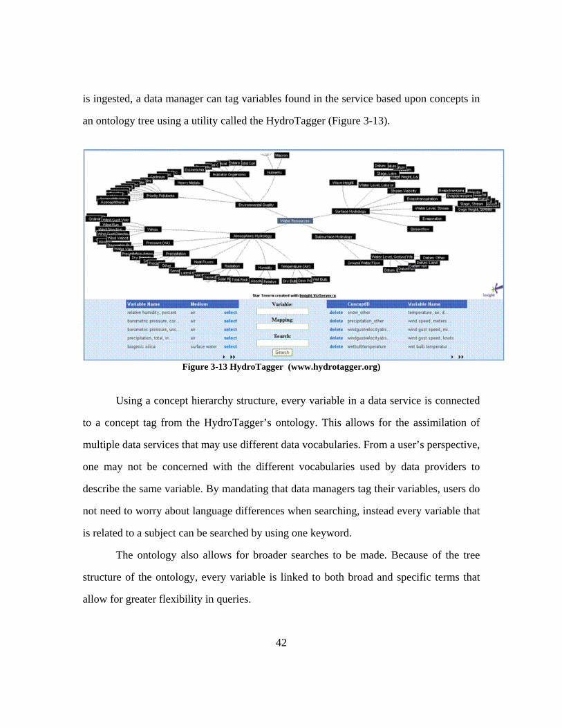
is ingested, a data manager can tag variables found in the service based upon concepts in
an ontology tree using a utility called the HydroTagger (Figure 3-13).
Figure 3-13 HydroTagger (www.hydrotagger.org)
Using a concept hierarchy structure, every variable in a data service is connected
to a concept tag from the HydroTagger’s ontology. This allows for the assimilation of
multiple data services that may use different data vocabularies. From a user’s perspective,
one may not be concerned with the different vocabularies used by data providers to
describe the same variable. By mandating that data managers tag their variables, users do
not need to worry about language differences when searching, instead every variable that
is related to a subject can be searched by using one keyword.
The ontology also allows for broader searches to be made. Because of the tree
structure of the ontology, every variable is linked to both broad and specific terms that
allow for greater flexibility in queries.
43
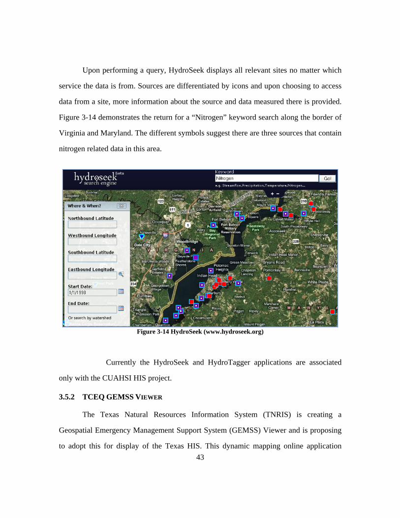
Upon performing a query, HydroSeek displays all relevant sites no matter which
service the data is from. Sources are differentiated by icons and upon choosing to access
data from a site, more information about the source and data measured there is provided.
Figure 3-14 demonstrates the return for a “Nitrogen” keyword search along the border of
Virginia and Maryland. The different symbols suggest there are three sources that contain
nitrogen related data in this area.
Figure 3-14 HydroSeek (www.hydroseek.org)
Currently the HydroSeek and HydroTagger applications are associated
only with the CUAHSI HIS project.
3.5.2 TCEQ GEMSS VIEWER
The Texas Natural Resources Information System (TNRIS) is creating a
Geospatial Emergency Management Support System (GEMSS) Viewer and is proposing
to adopt this for display of the Texas HIS. This dynamic mapping online application
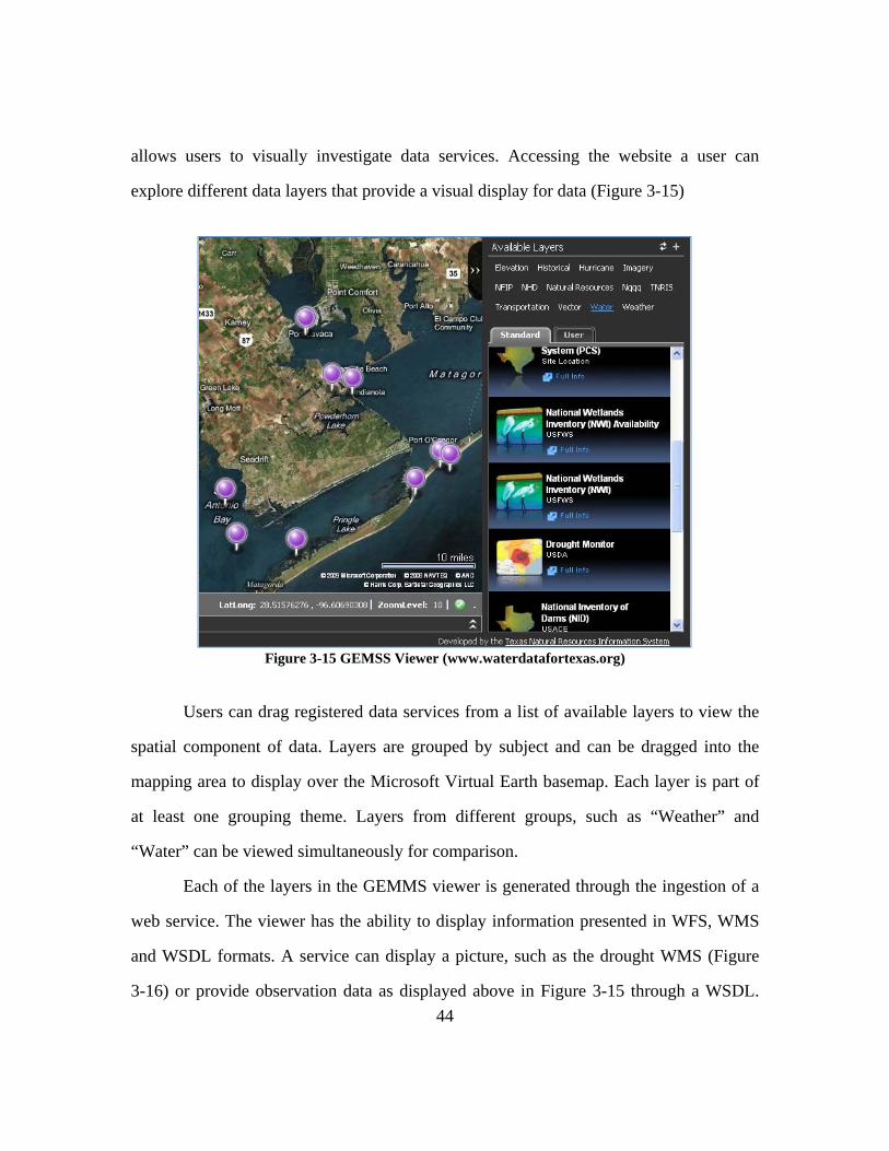
44
allows users to visually investigate data services. Accessing the website a user can
explore different data layers that provide a visual display for data (Figure 3-15)
Figure 3-15 GEMSS Viewer (www.waterdatafortexas.org)
Users can drag registered data services from a list of available layers to view the
spatial component of data. Layers are grouped by subject and can be dragged into the
mapping area to display over the Microsoft Virtual Earth basemap. Each layer is part of
at least one grouping theme. Layers from different groups, such as “Weather” and
“Water” can be viewed simultaneously for comparison.
Each of the layers in the GEMMS viewer is generated through the ingestion of a
web service. The viewer has the ability to display information presented in WFS, WMS
and WSDL formats. A service can display a picture, such as the drought WMS (Figure
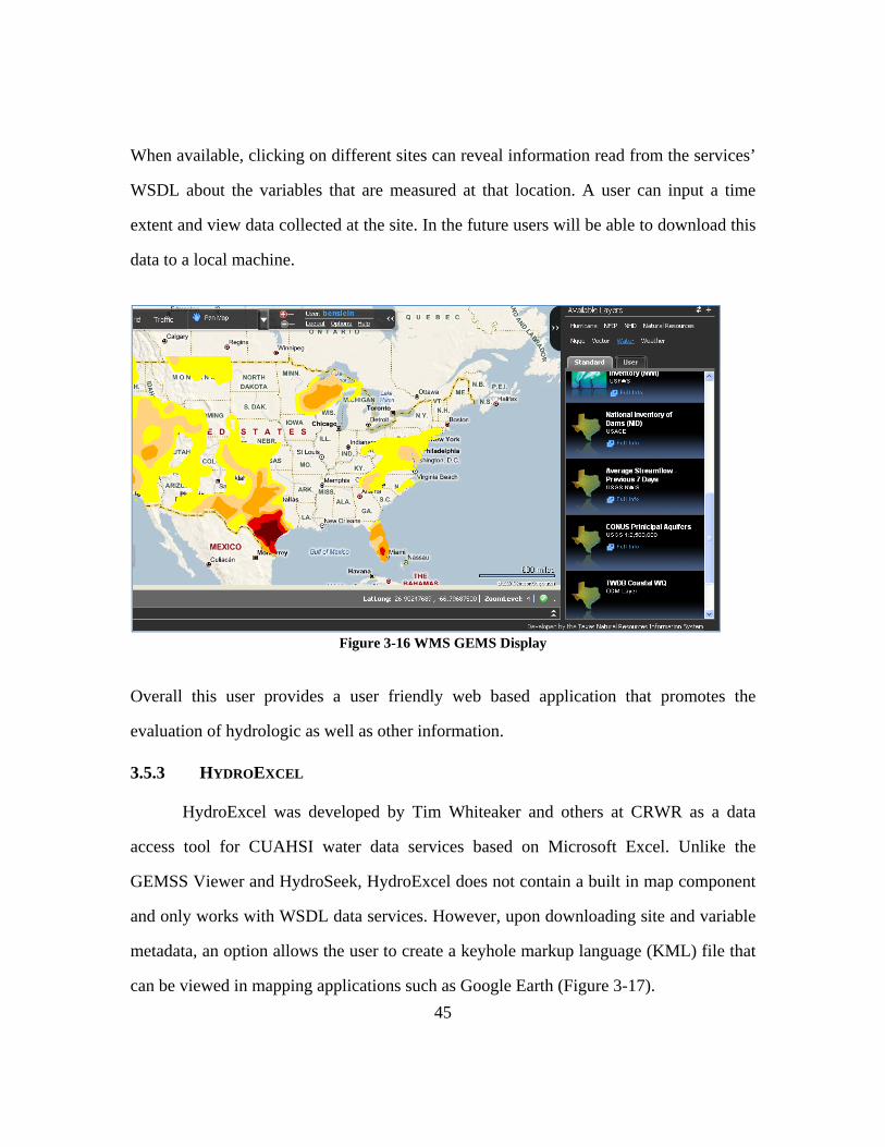
3-16) or provide observation data as displayed above in Figure 3-15 through a WSDL.
45
When available, clicking on different sites can reveal information read from the services’
WSDL about the variables that are measured at that location. A user can input a time
extent and view data collected at the site. In the future users will be able to download this
data to a local machine.
Figure 3-16 WMS GEMS Display
Overall this user provides a user friendly web based application that promotes the
evaluation of hydrologic as well as other information.
3.5.3 HYDROEXCEL
HydroExcel was developed by Tim Whiteaker and others at CRWR as a data
access tool for CUAHSI water data services based on Microsoft Excel. Unlike the
GEMSS Viewer and HydroSeek, HydroExcel does not contain a built in map component
and only works with WSDL data services. However, upon downloading site and variable
metadata, an option allows the user to create a keyhole markup language (KML) file that
can be viewed in mapping applications such as Google Earth (Figure 3-17).

46
Figure 3-17 TWDB Tides KML File
The spreadsheet allows for users, given a WSDL address, to search variable and
site metadata tables by calling the “Get Variables” and “Get Sites” service. Time series
data from each service can be downloaded and stored within the spreadsheet.
HydroExcel is able to interact with WaterOneFlow web services through a series
of macros embedded within the spreadsheet. These macros require a specific Dynamic
Link Library, known as HydroObjects, to be able to interpret the specific calls of
WaterOneFlow web services. Therefore HydroObjects is required to be downloaded and
installed from the his.cuahsi website before HydroExcel can function (Whiteaker, 2008)
47
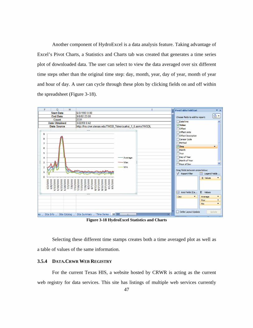
Another component of HydroExcel is a data analysis feature. Taking advantage of
Excel’s Pivot Charts, a Statistics and Charts tab was created that generates a time series
plot of downloaded data. The user can select to view the data averaged over six different
time steps other than the original time step: day, month, year, day of year, month of year
and hour of day. A user can cycle through these plots by clicking fields on and off within
the spreadsheet (Figure 3-18).
Figure 3-18 HydroExcel Statistics and Charts
Selecting these different time stamps creates both a time averaged plot as well as
a table of values of the same information.
3.5.4 DATA.CRWR WEB REGISTRY
For the current Texas HIS, a website hosted by CRWR is acting as the current
web registry for data services. This site has listings of multiple web services currently
48
being hosted by CRWR. The site is designed for users to explore the different types of
services offered and then allows them different avenues to access the data of each
service. A separate web page was created to provide details and a dynamic map for each
service.
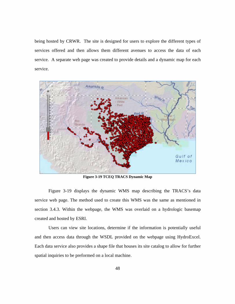
Figure 3-19 TCEQ TRACS Dynamic Map
Figure 3-19 displays the dynamic WMS map describing the TRACS’s data
service web page. The method used to create this WMS was the same as mentioned in
section 3.4.3. Within the webpage, the WMS was overlaid on a hydrologic basemap
created and hosted by ESRI.
Users can view site locations, determine if the information is potentially useful
and then access data through the WSDL provided on the webpage using HydroExcel.
Each data service also provides a shape file that houses its site catalog to allow for further
spatial inquiries to be preformed on a local machine.
49
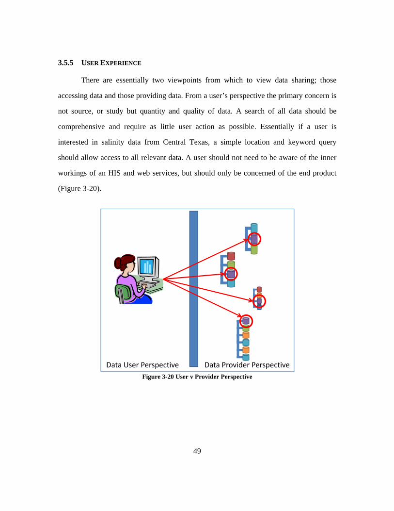
3.5.5 USER EXPERIENCE
There are essentially two viewpoints from which to view data sharing; those
accessing data and those providing data. From a user’s perspective the primary concern is
not source, or study but quantity and quality of data. A search of all data should be
comprehensive and require as little user action as possible. Essentially if a user is
interested in salinity data from Central Texas, a simple location and keyword query
should allow access to all relevant data. A user should not need to be aware of the inner
workings of an HIS and web services, but should only be concerned of the end product
(Figure 3-20).
Figure 3-20 User v Provider Perspective
Data User Perspective Data Provider Perspective

50
4 CASE STUDY OF THE TEXAS WATER DEVELOPMENT BOARD DATA PUBLICATION PROCESS
The Texas Water Development Board (TWDB) compiled a list of databases for
CRWR to upload into the ODM and aid in hosting as part of the Texas HIS project. This
section examines the publication process of several of the TWDB Major and Special
Field Studies data sets. These studies include six different data sets from 14 bays along
the Texas Coast and include data measured from 1987 to 1997 (Figure 4-1).
Figure 4-1 TWDB Field Study Locations
www.twdb.state.tx.

51
The data sets that are examined in this case study are the TWDB Datasondes,
Water Quality and Tides Data. The different methods that were used to upload these data
sets represent an interesting comparison for the data publication process.
The Datasondes data arose from a series of studies performed by implementing
data monitoring sondes throughout the Texas Bays. Dataondes are digital monitoring
devices that are able to measure and store continuous data of multiple parameters
simultaneously. The TWDB Datasondes study measured pH, temperature, conductivity,
salinity and dissolved oxygen.
Figure 4-2 Datasonde
In total there were 56 sites in which datasonde measurements were loaded into the ODM.
The majority of these sites measured all five of the previously mentioned variables. In
total over 117,000 data values of these variables were measured.

52
The TWDB Water Quality Studies were very similar to the datasondes studies in
the variables measured. The identical 5 measurements were taken as well as the depth at
which the measurement was made. In total 141 sites were monitored and over 86,000
data values were recorded from 14 different studies spanning from 1987 to 1997.
The TWDB Tides Studies were performed to measure the variability of tides at
105 different sites along the coast. Each measurement was made against an arbitrary
datum and recorded on an hourly interval. In total over 65,000 gage heights were
recorded.
4.1 TWDB Data Background
4.1.1 TWDB DATA STRUCTURE
This data was made available to CRWR by the delivery of a compact disc with
several folders containing studies of interest. Data was stored by the TWDB based on a
year and location and not individual study. Figure 4-3 demonstrates the hierarchy of how
data was housed within the CD sent by TWDB. Each level of hierarchy demonstrates a
folder that contained the information listed under it.
53
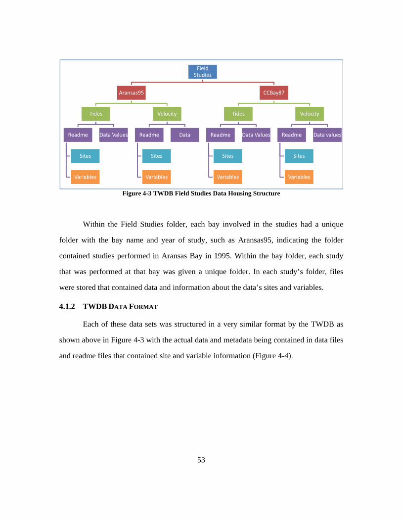
Figure 4-3 TWDB Field Studies Data Housing Structure
Within the Field Studies folder, each bay involved in the studies had a unique
folder with the bay name and year of study, such as Aransas95, indicating the folder
contained studies performed in Aransas Bay in 1995. Within the bay folder, each study
that was performed at that bay was given a unique folder. In each study’s folder, files
were stored that contained data and information about the data’s sites and variables.
4.1.2 TWDB DATA FORMAT
Each of these data sets was structured in a very similar format by the TWDB as
shown above in Figure 4-3 with the actual data and metadata being contained in data files
and readme files that contained site and variable information (Figure 4-4).
Field Studies
Aransas95
Tides
Readme
Sites
Variables
Data Values
Velocity
Readme
Sites
Variables
Data
CCBay87
Tides
Readme
Sites
Variables
Data Values
Velocity
Readme
Sites
Variables
Data values

54
Figure 4-4 Example TWDB Readme File
Each site had a “station” number, name, latitude and longitude and the variables
measured at the sites were mentioned and given a unit of measurement. The station
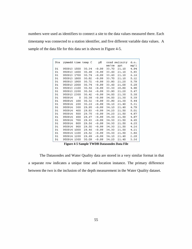
55
numbers were used as identifiers to connect a site to the data values measured there. Each
timestamp was connected to a station identifier, and five different variable data values. A
sample of the data file for this data set is shown in Figure 4-5.
Figure 4-5 Sample TWDB Datasondes Data File
The Datasondes and Water Quality data are stored in a very similar format in that
a separate row indicates a unique time and location instance. The primary difference
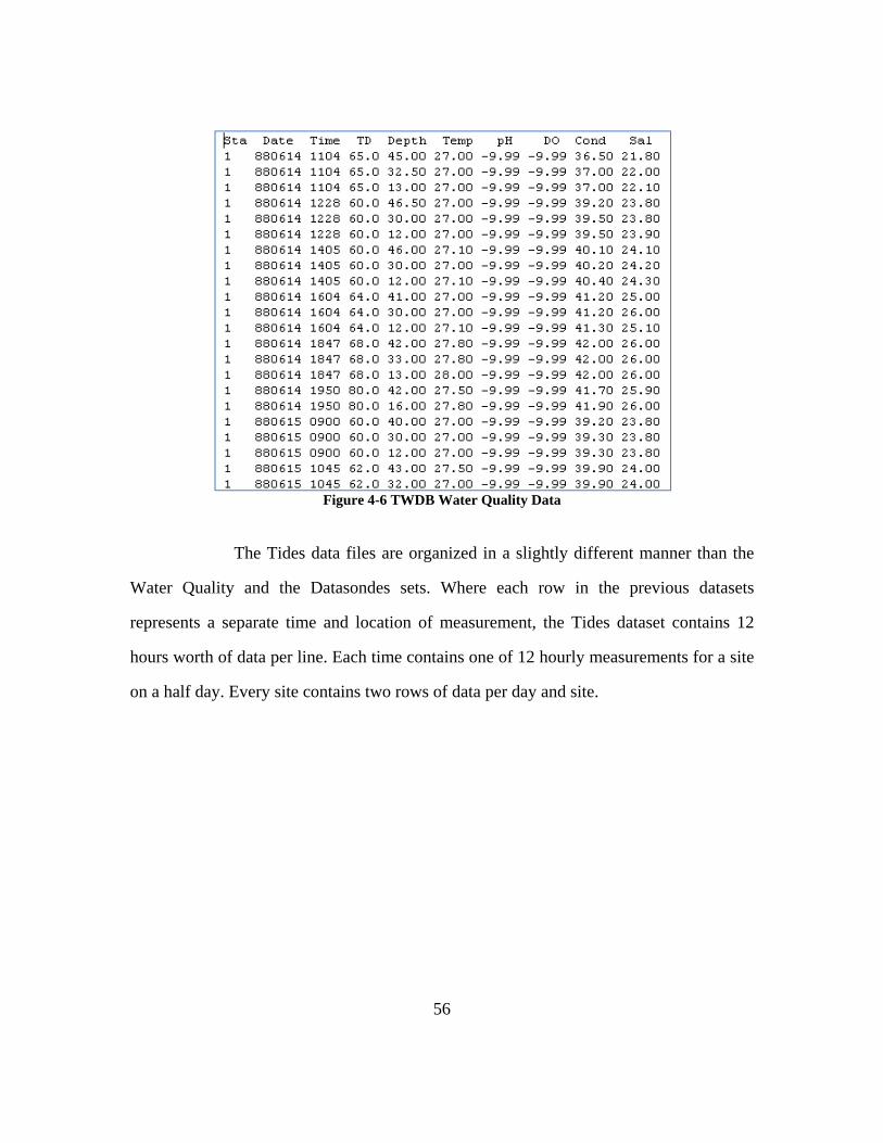
between the two is the inclusion of the depth measurement in the Water Quality dataset.
56
Figure 4-6 TWDB Water Quality Data
The Tides data files are organized in a slightly different manner than the
Water Quality and the Datasondes sets. Where each row in the previous datasets
represents a separate time and location of measurement, the Tides dataset contains 12
hours worth of data per line. Each time contains one of 12 hourly measurements for a site
on a half day. Every site contains two rows of data per day and site.

57
Figure 4-7 TWDB Tides Sample Data
From this point, two different approaches were taken in loading data into the
ODM. SSIS was used to upload both the Datasondes and Water Quality data, while the
Tides data set was uploaded with the ODM Data Loader.
4.2 Distinct ODM Data Services
The TWDB’s Datasondes, Water Quality and Tides data sets were loaded into a
unique ODM database using either the SSIS or ODM Data Loader method. This decision
to house each study within different databases was founded by the belief that though one
source may produce multiple sets of data, data from the same source does not need to be
grouped together within a single database. Having each data set be housed in a separate
database distinguishes the differences between services and creates an organizational
structure within an HIS. Each source may have multiple databases that contain unique
data, and these sources are all brought together under the HIS umbrella (Figure 4-8).

58
Figure 4-8 HIS Data Hierarchy
Though each of these studies was housed within a separate ODM, the creation of
thematic layers and a comprehensive HIS metadata catalog reduces the importance of
separating individual studies and even sources. Within the ODM each data value can be
linked to a SamplingID that associates a measurement to a particular study, as well as a
SourceID that links to a single source.
As long as each dataset that is loaded into an ODM is hosted in the same method,
as opposed to having a dataset be part of a hybrid service, and contains the same
vocabulary, there is no limit to the amount of sources or studies that can be housed within
the ODM. A data manager may want to limit the data inserted into the ODM based on
ease of managing the service and the amount of time it takes for a user to access the
information within a service. A data service with massive amounts of site and variable
information will take proportionally longer for an application to access than an ODM
with less information.
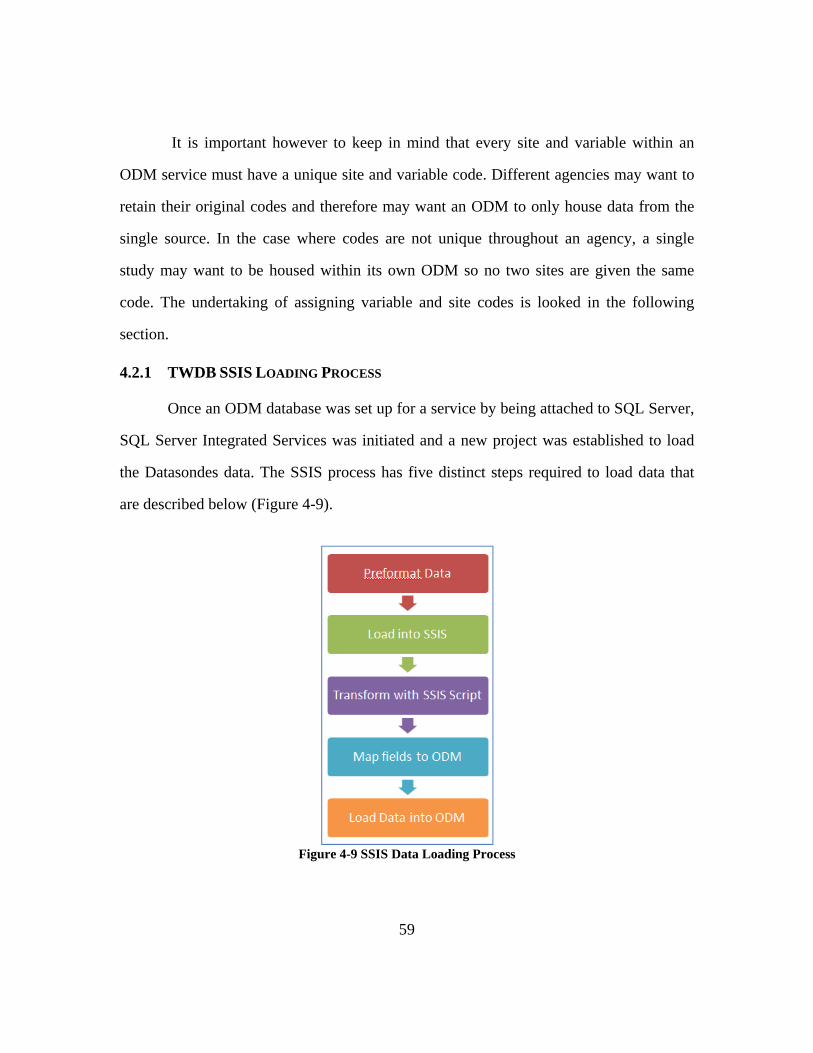
59
It is important however to keep in mind that every site and variable within an
ODM service must have a unique site and variable code. Different agencies may want to
retain their original codes and therefore may want an ODM to only house data from the
single source. In the case where codes are not unique throughout an agency, a single
study may want to be housed within its own ODM so no two sites are given the same
code. The undertaking of assigning variable and site codes is looked in the following
section.
4.2.1 TWDB SSIS LOADING PROCESS
Once an ODM database was set up for a service by being attached to SQL Server,
SQL Server Integrated Services was initiated and a new project was established to load
the Datasondes data. The SSIS process has five distinct steps required to load data that
are described below (Figure 4-9).
Figure 4-9 SSIS Data Loading Process

60
Since data from every bay was contained in separate folders, individual
connections had to be made to access the data in each folder. Each separate folder,
representing a different set of locations, had to have a unique loading process into the
ODM. Thus the described process was repeated for each folder in the study. Once
connected to the data files, SSIS then had to be told how to parse out and name each
column through its “Flat File Connection Manager Editor”.
Figure 4-10 SSIS Connection Manager
Once a data file was connected to SSIS it was able to be transformed through
SSIS script. Since the ODM requires the sites metadata to be populated prior to the data

61
values table, the SSIS sequence of loading site data must be implemented before the data
values sequence. The small amount of data that needed to be loaded into the variables
table, a total of five variables, was manually loaded into the ODM manually instead of
using any data loader; this also pertained to the source and methods tables. This involved
opening the actual ODM tables outside of the SSIS program and typing in the specific
fields that were updated. Since the original data contained very little variable metadata,
for SSIS or ODM Data Loader to load any information into the ODM, a table would have
had to be created within Excel. Thus inputting this data into the ODM manually proved to
be the most effective method of populating a variables table.
SSIS has the ability to use “scripts” to transform data. These scripts are just lines
of Visual Basic code that can be used to manipulate data. For this data, the script used to
transform the sites data into the correct format, found in the SSIS loading process in
Appendix C, needed only to convert a site’s latitude and longitude from degrees, minutes,
seconds into decimal degree notation and provide metadata information for required
fields. These fields were State, County, LatlongdatumID and SiteID. Both state and
county can be determined by the latitude and longitude of each site and the
LatlongdatumID, referring to the coordinate datum, was found to be based off The North
American Datum of 1983 represented with the identifier of “2” in the ODM’s Spatial
References table.
The final metadata field filled, SiteCode, was one that received considerable
amounts of thought. Both SiteCode and VariableCode are unique identifiers used to
identify each site and variable. These codes are intended to be assigned based on an
agency’s coding. For example the USGS has numeric codes for each variable it measures
one of which, 0060, stands for mean daily streamflow in every study it performs.
However, The TWDB did not possess either SiteCodes or VariableCodes it could suggest

62
to use. Effort was made by both CRWR and TWDB to come up with codes that could
work for every site within the agency. In the end no standardized solution was found that
was appropriate to apply for every study’s SiteCodes. Due to the large number of sites
studied within the TWDB organization, no single method of coding sites was deemed
suitable to standardize their site code methodology. It was decided that each code was
then implemented in a case by case basis. Different studies would then contain different
information that would go into the building of a site code. For example, a number of
studies were given site codes based on the bay the study was located within and then the
specific station number given to a specific site by the TWDB.
VariableCodes were implemented that could apply to every variable measured in
these studies. These codes are a combination of three upper case letters followed by three
numbers. The letter configuration is a representation of a variable group. As an example,
all variables with the prefix SOL deal with variations of Solids such as Total Dissolved
Solids (SOL004) and Suspended Solids (SOL002). The three digit suffix signifies the
association with a larger group and has no additional meaning. All variables that deal
with Solids share the common SOL prefix and the suffix 001 to 009 to distinguish
between variations of Solid variables. However, with the implementation of the ODM
1.1’s controlled vocabulary and a CUAHSI ontology, it seems as though there is little
importance of a standardized VariableCode outside of a given agency’s in-house use.
The SiteCodes for the Datasondes dataset were eventually created based on
TWDB’s station identifiers a three number identifier TWDB gave to a majority of sites.
The assigning of these codes was performed through the SSIS sites script.
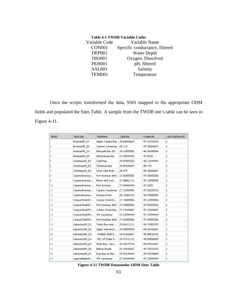
63
Table 4-1 TWDB Variable Codes Variable Code Variable Name
CON001 Specific conductance, filtered DEP001 Water Depth DIO001 Oxygen, Dissolved PEH001 pH, filtered SAL001 Salinity TEM001 Temperature
Once the scripts transformed the data, SSIS mapped to the appropriate ODM
fields and populated the Sites Table. A sample from the TWDB site’s table can be seen in
Figure 4-11.
Figure 4-11 TWDB Datasondes ODM Sites Table
64
The loading of data values using SSIS was similar to the sites process in that
multiple connections had to be made to the different data files. Upon uploading this data
with SSIS, data files had to be double checked continually to ensure that no formatting
errors were made in the upload. An example of this is an incorrectly aligned row, causing
for data to be placed in the wrong columns within the ODM. Scripts were also used to
convert the date time format into one recognized by the ODM. The most efficient method
in checking to ensure the data was loaded correctly was through finding random dates
throughout the ODM DataValues table and ensuring the connecting values matched with
those in the original data sets provided by TWDB.
This same process was later repeated with data from the TWDB Water Quality
data set. Since the data was so similar the process was nearly identical. However,
between loading the two datasets the ODM Version 1.1 was developed. One change in
this database was the automated population of the ID fields in each table, such as
ValueID and SiteID. In using the ODM Data Loader 1.1 this advancement is not a
problem since data values can be linked to tables through site and variable codes and the
ODM Data Loader then automatically populates the ODM and inputs correct IDs.
However loading data with SSIS still required data values to link to other tables using
only SiteIDs and VariableIDs. Therefore the site and variable tables had to be loaded
correctly before the data values script could be written. A common problem occurred
when editing metadata after it was loaded into the ODM 1.1. When deleting a row, the ID
given to it is no longer able to be used by other rows of data. If a row was deleted for
editing purposes and then reloaded into the ODM, a new ID would be assigned to the row
and any previous link to that ID would be broken. For this reason all ID’s must be final
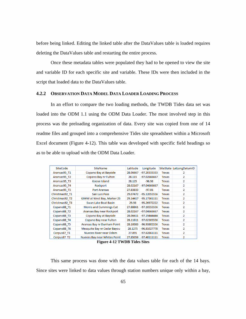
65
before being linked. Editing the linked table after the DataValues table is loaded requires
deleting the DataValues table and restarting the entire process.
Once these metadata tables were populated they had to be opened to view the site
and variable ID for each specific site and variable. These IDs were then included in the
script that loaded data to the DataValues table.
4.2.2 OBSERVATION DATA MODEL DATA LOADER LOADING PROCESS
In an effort to compare the two loading methods, the TWDB Tides data set was
loaded into the ODM 1.1 using the ODM Data Loader. The most involved step in this
process was the preloading organization of data. Every site was copied from one of 14
readme files and grouped into a comprehensive Tides site spreadsheet within a Microsoft
Excel document (Figure 4-12). This table was developed with specific field headings so
as to be able to upload with the ODM Data Loader.
Figure 4-12 TWDB Tides Sites
This same process was done with the data values table for each of the 14 bays.
Since sites were linked to data values through station numbers unique only within a bay,

66
in importing data values into the spreadsheet it was important to create an extra row of
data that tracked from which bay study the data came from. Station numbers had to be
combined with the bay name and year, ie Aransas95, to identify each unique site. This
combination of bay, year and station number was used to create unique site codes for the
data. Excel was also used to transform the date time format (yyddmm tttt) into one
recognized by the ODM (mm/dd/yyyy tt:tt). Once these changes were made, the Sites
Table and then the DataValues Table were uploaded using the ODM Data Loader (Figure
4-13).
Figure 4-13 ODMDL of TWDB Tide Data Values
This tide data measured one variable, gage height, from one source, TWDB, using
one method. This was again an example of a time when it was simpler to directly input
data manually into the Variables and Methods ODM tables than using a data loader. A
key feature in the ODM Data Loader is its ability to link data values to sites and variables
by SiteCode and VariableCode, and not rely on SiteID and VariableID. In this case the
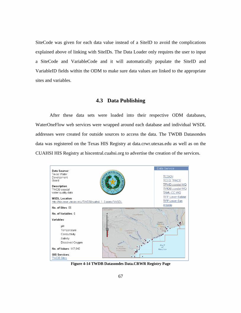
67
SiteCode was given for each data value instead of a SiteID to avoid the complications
explained above of linking with SiteIDs. The Data Loader only requires the user to input
a SiteCode and VariableCode and it will automatically populate the SiteID and
VariableID fields within the ODM to make sure data values are linked to the appropriate
sites and variables.
4.3 Data Publishing
After these data sets were loaded into their respective ODM databases,
WaterOneFlow web services were wrapped around each database and individual WSDL
addresses were created for outside sources to access the data. The TWDB Datasondes
data was registered on the Texas HIS Registry at data.crwr.utexas.edu as well as on the
CUAHSI HIS Registry at hiscentral.cuahsi.org to advertise the creation of the services.
Figure 4-14 TWDB Datasondes Data.CRWR Registry Page
68
The data.crwr page displayed all basic information about the data service such as
variables included, number of sites and the source of the data and allowed for viewing of
each individual site on a dynamic map.
At the time this document was written, final quality checks were being applied to
each TWDB data service to ensure data quality. Eventually each data service created will
be featured on the data.crwr web site as well as ingested in the CUASHI HIS Central and
HIS Registry. Ultimately the ODMs populated with the different data sets will be hosted
by an HIS server at TWDB on what will be a more permanent server than the test server
at CRWR.
69
5 CONCLUSIONS
The efforts put forth by the CUAHSI and CRWR HIS teams have already
improved the availability of data within the hydrologic community. Leading by example,
they have demonstrated that it is possible to integrate large and small data sets across the
field of hydrologic science. The ability to replicate this process with governmental
agencies on a Texas scale is an indication that the HIS framework has an extremely
strong and promising future.
What are the different roles played in a Texas HIS compared to a national HIS?
A state or regional HIS can focus on gathering smaller data sets that may be
overlooked on a national scale. These data sets, though of a lesser size, are of no lesser
importance to the achievement of advancing hydrologic science. While a national HIS
should have connections with national data collection agencies such as the EPA and
USGS, a state HIS can develop relationships with statewide data collection agencies that
may be too small to be of interest to a national system. These relationships are vital for a
state HIS so as to develop a tailored product based off user needs, all the while being able
to rely on the framework provided by the national HIS project.
What are the greatest difficulties in creating a Texas HIS and how can these be
overcome?
At this stage of development, the greatest obstacle to overcome in creating an HIS
of any scale is the involvement of outside agencies in providing and hosting data. As with
70
any new technology, it is extremely important to attract users from varied outside
communities. As mentioned above, the implementation of different scales of an HIS
facilitates the identification of data providers and users of the system. An HIS data
manager can work with agencies on the same scale of the HIS to identify the needs of the
particular system. A successful HIS should be in constant dialog with all involved parties
to constantly improve the services it offers.
What lessons have been learned in the data loading process?
One major improvement since the initiation of the Texas HIS was the
understanding of the data loading process. The learning curve that was needed to grasp
the workings of loading data with SSIS was substantial and required many attempts
before a workable method could be created. This also led to greater appreciation for the
use of the ODM Data Loader. Though loading with SSIS was eventually successful, the
effort and time taken in learning the program does not facilitate the loading of data. For
this reason the ODM Data Loader should continue to play a very important role in the
development and spread of the Texas HIS.
In choosing one method over another, one should consider what type of data is
being loaded and the future of loading data. If multiple data files that need significant
transformation are to be loaded into the ODM, using SSIS may prove to be the more
efficient method. Since these transformations can be performed through a script that can
be accessed every time data is loaded, this would require less time than repeating the
same functions in Excel for each data file. However, in most cases using the ODM Data
Loader should be recommended over the more technical SSIS. The Data Loader requires
a minimum level of data quality prior to loading into the ODM by checking for duplicate

71
rows, null data values and appropriate linkages between tables. The amount of time
required to learn the ODM Data Loader loading process is also greatly reduced from that
of the SSIS. The user interface is very straight forward and requires limited input by the
user. A collection of loaded data can be found on the data.crwr.utexas.edu website. These
sets were all loaded using SSIS however, for quality control many are being reloaded
using the Data Loader. In the future, most datasets will be loaded with the ODM Data
Loader due to this quality control level and transparency in the loading process.
Another important lesson learned concerned working with multiple datasets from
multiple agencies. It was important to frequently run quality control checks on every
aspect of the HIS to ensure the integrity of the hosted data. This involves checking the
performance of each service as well as the content. While working on the Texas HIS
server prototype it was difficult to regularly update both the ODMs and web services with
the new technology being implemented. Without the implementation of different levels of
an HIS, it would be impossible to ensure any level of quality for each data service due to
the amount of services being offered.
Working with data from outside sources also results in a knowledge gap between
data collectors and data loaders. Even with open communication between a data loader
and data collector, a data loader will not understand a dataset as well as one who was
involved in the collection of the actual measurements. Thus how a data loader and data
collector would populate an ODM’s metadata tables may differ. For this reason it would
be ideal for those who are responsible for data collection also be responsible for data
loading. This can become a reality as long as user friendly applications, such as the ODM
Data Loader, are made available.

72
What technologies are currently being utilized in creating a Texas HIS?
A benefit of a state HIS based off a national scale system is the technology and
knowledge one can contribute to the other. The implementation of the ODM Data
Loader, developed as part of the national HIS project, has facilitated the loading of
multiple lesser scale data sets. The desire to access specific data services directly led to
the development of HydroExcel, an application that works especially well for the smaller
regional and statewide services rather than those with thousands of different sites. The
desire to use HydroExcel to query based on geographic location led to the development
of new web services that allow for bounding box queries. These web services, in return,
allow HydroExcel to access large datasets in a more manageable way. This is an example
of products developed for use in a state wide system influencing the development of
national products and vice versa. The success of the Texas HIS as well as the national
HIS is due in part to the sharing of these technologies. Specifically, the continued
development of the ODM, ODM Data Loader, and multiple data discovery applications
such as HydroExcel and HydroSeek is important to the current, as well as future,
implementation of the HIS on all levels.
5.1 Recommendations for Future Research
An area where more research is needed is in the implementation of integrated
services such as the Salinity Service described in section 3.4.6. These integrated services
73
allow for users to search beyond the resources that a single data service can provide and
places the importance of data over the importance of source.
One vital aspect of creating these services is the quality of data. Though users
may like to overlook the source of data, it is the responsibility of an HIS manger to
provide not only quantity but transparency in the quality of data. In this way a data
manager must be strict in adhering to the quality control level inputs within the ODM. It
may be beneficial to allow for integrated services to be built on multiple quality control
levels so that the highest level of quality control will yield results from the most reputable
sources such as the USGS and EPA. In that way, any source of data can be ingested into
an HIS and integrated service without compromising the overall integrity of all services
offered.
Allowing for any level of quality controlled data to be included in an HIS is also
important to its expansion. Though large “trusted” data sets are of vital importance, the
significant contribution of a smaller scale HIS is in the publication of regional and
statewide studies. These regional data sets must be encouraged to publish data through
hosting their own data service or through submitting data to an agency, such as CRWR,
that will create and host a service for them. For this reason, data loading and hosting
seminars must be offered throughout the areas that an HIS covers. Without these
seminars it is impossible to know the extent of data that is available to an HIS.
With encouraging potential data managers to host data comes the need to continue
to simplify the data upload process. As discussed in section 3.3 the SSIS uploading
methodology can be overwhelming for a novice data loader, therefore the ODM Data
Loader should be recommended method for initial data loads. With encouraging the use
of the ODM Data Loader the use of the ODM as the primary database in an HIS must
also be encouraged. Through increased use of both the ODM and ODM Data Loader, it is
74
important to continually ask for user feedback and update both products to suit user
needs.
The greatest lesson that can be taken away from the continued development of
any scale of an HIS is the importance of user driven product development and
implementation. The technologies that allow for data services to be created and integrated
under the HIS prove to be a great step forward in the field of hydroinformatics. However,
these technologies are only as good as the services they provide the end user. In
evaluating similar HIS efforts in section 2.2, the factor that was most influential in
making an assessment of the system was not the data it housed or available features.
Instead it was the ease in which a task could be performed. Both the data.crwr web page
and CUAHSI Hydroseek demonstrate a product that is very intuitive for its users and this
functionality, above the amount of data or tools within an HIS, is the key aspect in
designing a successful product. The implementation of the GEMSS Viewer will provide
the Texas HIS with a greater data discovery experience and encourage greater public use
by again providing a tool that is both useful and intuitive for the user.
The potential of any size HIS is only as great as the energy that goes into
promoting the project. Though it is important to continue to make improvements, the
greatest advancement that can currently be made is the emergence of more regional and
statewide HISs as well as contributions the CUAHSI HIS. The technology for this system
is at the implementation level and throughout the country governmental, industrial and
academic institutions should be encouraged to form regional and statewide HIS
committees. The HIS projects have reached a state where success is no longer a function
of technological advances but of the participation of the hydrologic community.
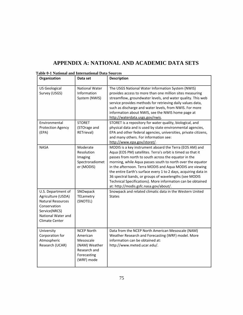
75
APPENDIX A: NATIONAL AND ACADEMIC DATA SETS
Table 0-1 National and International Data Sources Organization Data set Description
US Geological Survey (USGS)
National Water Information System (NWIS)
The USGS National Water Information System (NWIS) provides access to more than one million sites measuring streamflow, groundwater levels, and water quality. This web service provides methods for retrieving daily values data, such as discharge and water levels, from NWIS. For more information about NWIS, see the NWIS home page at http://waterdata.usgs.gov/nwis.
Environmental Protection Agency (EPA)
STORET (STOrage and RETrieval)
STORET is a repository for water quality, biological, and physical data and is used by state environmental agencies, EPA and other federal agencies, universities, private citizens, and many others. For information see: http://www.epa.gov/storet/.
NASA Moderate Resolution Imaging Spectroradiometer (MODIS)
MODIS is a key instrument aboard the Terra (EOS AM) and Aqua (EOS PM) satellites. Terra's orbit is timed so that it passes from north to south across the equator in the morning, while Aqua passes south to north over the equator in the afternoon. Terra MODIS and Aqua MODIS are viewing the entire Earth's surface every 1 to 2 days, acquiring data in 36 spectral bands, or groups of wavelengths (see MODIS Technical Specifications). More information can be obtained at: http://modis.gsfc.nasa.gov/about/.
U.S. Department of Agriculture (USDA) Natural Resources Conservation Service(NRCS) National Water and Climate Center
SNOwpack TELemetry (SNOTEL)
Snowpack and related climatic data in the Western United States
University Corporation for Atmospheric Research (UCAR)
NCEP North American Mesoscale (NAM) Weather Research and Forecasting (WRF) mode
Data from the NCEP North American Mesoscale (NAM) Weather Research and Forecasting (WRF) model. More information can be obtained at: http://www.meted.ucar.edu/.
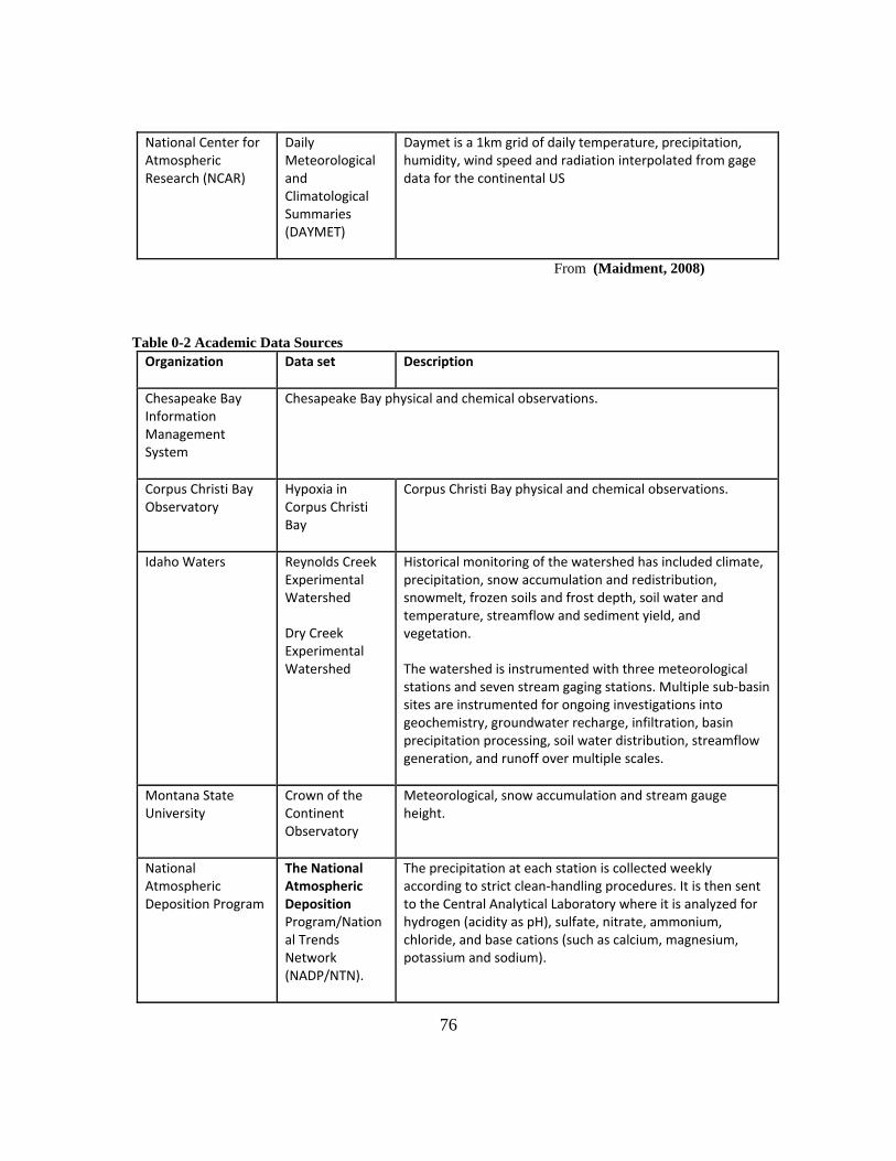
76
National Center for Atmospheric Research (NCAR)
Daily Meteorological and Climatological Summaries (DAYMET)
Daymet is a 1km grid of daily temperature, precipitation, humidity, wind speed and radiation interpolated from gage data for the continental US
From (Maidment, 2008) Table 0-2 Academic Data Sources Organization Data set Description
Chesapeake Bay Information Management System
Chesapeake Bay physical and chemical observations.
Corpus Christi Bay Observatory
Hypoxia in Corpus Christi Bay
Corpus Christi Bay physical and chemical observations.
Idaho Waters Reynolds Creek Experimental Watershed
Dry Creek Experimental Watershed
Historical monitoring of the watershed has included climate, precipitation, snow accumulation and redistribution, snowmelt, frozen soils and frost depth, soil water and temperature, streamflow and sediment yield, and vegetation.
The watershed is instrumented with three meteorological stations and seven stream gaging stations. Multiple sub‐basin sites are instrumented for ongoing investigations into geochemistry, groundwater recharge, infiltration, basin precipitation processing, soil water distribution, streamflow generation, and runoff over multiple scales.
Montana State University
Crown of the Continent Observatory
Meteorological, snow accumulation and stream gauge height.
National Atmospheric Deposition Program
The National Atmospheric Deposition Program/National Trends Network (NADP/NTN).
The precipitation at each station is collected weekly according to strict clean‐handling procedures. It is then sent to the Central Analytical Laboratory where it is analyzed for hydrogen (acidity as pH), sulfate, nitrate, ammonium, chloride, and base cations (such as calcium, magnesium, potassium and sodium).

77
San Diego River Park Foundation
Meteorology and hydrology observations
Susquehanna River Basin Hydrologic Observatory System
Meteorology, air and hydrology observations
Suwannee River Water Management District
Ground Water Levels
Groundwater level (GWL) records are available for 1,089 wells. The majority of these wells are only measured during record high or record low periods and 396 wells are inactive. One hundred and eighty‐one (181) wells are measured monthly in the GWL network; of these, 77 have continuous recorders. Groundwater levels are stored in the District’s GWL database. In feet above NGVD29
Texas Commission for Environmental Quality
TRACS TRACS (TCEQ Regulatory Activities and Compliance System) water quality data
Texas Instream Flow Program
Lower Sabine Biological fish species and aquatic environment data from the lower Sabine River, Texas
Texas Parks and Wildlife Department
Coastal water surveys
Water Level, turbidity, salinity, temperature, and dissolved oxygen levels.
University of Florida Water Institute
Waters Testbed Project
Data from nitrate sensor: YSI 9600 Nitrate Monitor allows a user to continuously record nitrate levels at a variable sample interval and providing improved detection of nitrate dynamics vis‐a‐vis grab sampling.
University of Iowa Clear Creek Precipitation
University of North Carolina
Ferry Mon, Albemarle‐Pamlico Sound
Water quality observations
Utah State University
Little Bear River WATERSTest Bed
Mud Lake
Continuous water quality monitoring of the Little Bear River to investigate the use of surrogate measures such as turbidity in creating high frequency load estimates for constituents that cannot be measured continuously.
Continuous water quality monitoring to investigate the sediment and nutrient budget of Mud Lake within the Bear Lake National Wildlife Refuge, Idaho.
From (Maidment, 2008)
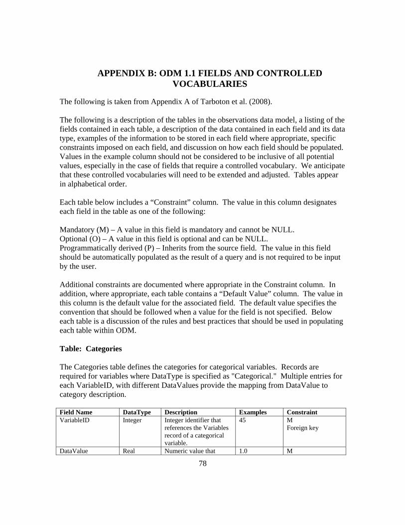
78
APPENDIX B: ODM 1.1 FIELDS AND CONTROLLED VOCABULARIES
The following is taken from Appendix A of Tarboton et al. (2008). (Tarboton et al, 2008) The following is a description of the tables in the observations data model, a listing of the fields contained in each table, a description of the data contained in each field and its data type, examples of the information to be stored in each field where appropriate, specific constraints imposed on each field, and discussion on how each field should be populated. Values in the example column should not be considered to be inclusive of all potential values, especially in the case of fields that require a controlled vocabulary. We anticipate that these controlled vocabularies will need to be extended and adjusted. Tables appear in alphabetical order. Each table below includes a “Constraint” column. The value in this column designates each field in the table as one of the following: Mandatory (M) – A value in this field is mandatory and cannot be NULL. Optional (O) – A value in this field is optional and can be NULL. Programmatically derived (P) – Inherits from the source field. The value in this field should be automatically populated as the result of a query and is not required to be input by the user. Additional constraints are documented where appropriate in the Constraint column. In addition, where appropriate, each table contains a “Default Value” column. The value in this column is the default value for the associated field. The default value specifies the convention that should be followed when a value for the field is not specified. Below each table is a discussion of the rules and best practices that should be used in populating each table within ODM. Table: Categories The Categories table defines the categories for categorical variables. Records are required for variables where DataType is specified as "Categorical." Multiple entries for each VariableID, with different DataValues provide the mapping from DataValue to category description. Field Name DataType Description Examples Constraint VariableID Integer Integer identifier that
references the Variables record of a categorical variable.
45 M Foreign key
DataValue Real Numeric value that 1.0 M

79
defines the category CategoryDescription Text
(Unlimited) Definition of categorical variable value
“Cloudy” M
The following rules and best practices should be used in populating this table:
1. Although all of the fields in this table are mandatory, they need only be populated if categorical data are entered into the database. If there are no categorical data in the DataValues table, this table will be empty.
2. This table should be populated before categorical data values are added to the DataValues table.
Table: CensorCodeCV The CensorCodeCV table contains the controlled vocabulary for censor codes. Only values from the Term field in this table can be used to populate the CensorCode field of the DataValues table. Field Name Data Type Description Examples Constraint Term Text (255) Controlled vocabulary
for CensorCode. “lt”, “gt”, “nc” M
Unique Primary key Cannot contain tab, line feed, or carriage return characters
Definition Text (unlimited)
Definition of CensorCode controlled vocabulary term. The definition is optional if the term is self explanatory.
“less than”, “greater than”, “not censored”
O
This table is pre-populated within the ODM. Changes to this controlled vocabulary can be requested at http://water.usu.edu/cuahsi/odm/. Table: DataTypeCV The DataTypeCV table contains the controlled vocabulary for data types. Only values from the Term field in this table can be used to populate the DataType field in the Variables table.
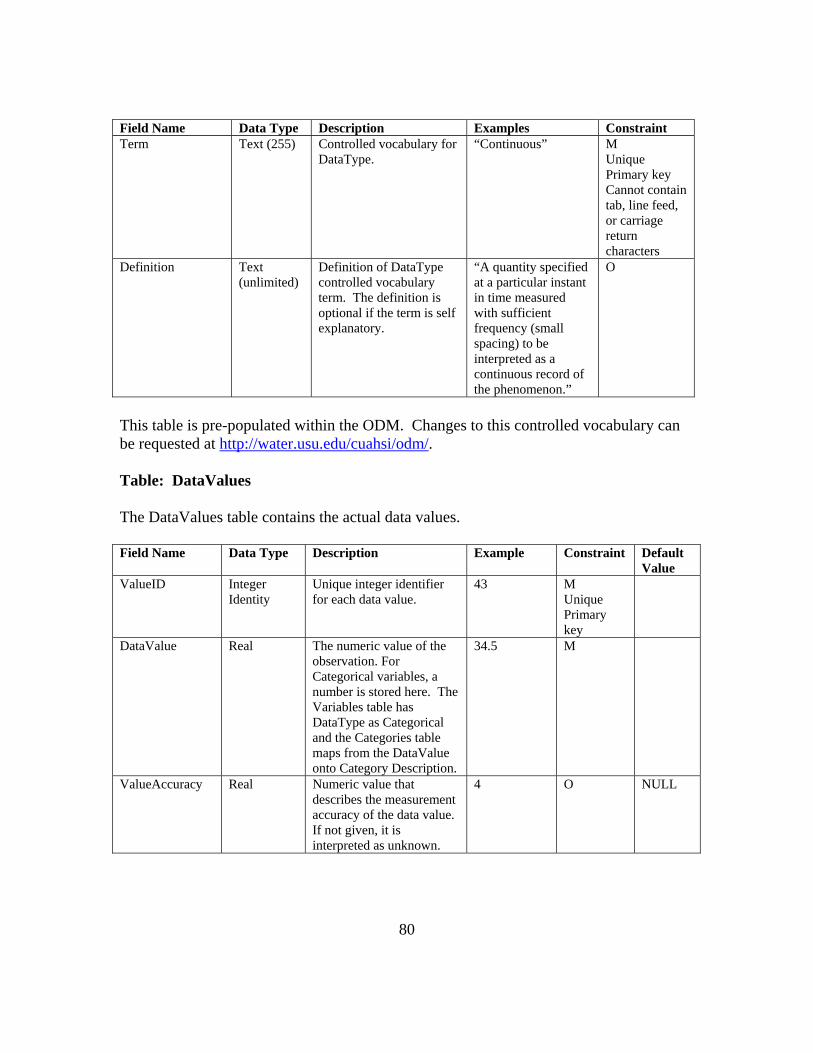
80
Field Name Data Type Description Examples Constraint Term Text (255) Controlled vocabulary for
DataType. “Continuous” M
Unique Primary key Cannot contain tab, line feed, or carriage return characters
Definition Text (unlimited)
Definition of DataType controlled vocabulary term. The definition is optional if the term is self explanatory.
“A quantity specified at a particular instant in time measured with sufficient frequency (small spacing) to be interpreted as a continuous record of the phenomenon.”
O
This table is pre-populated within the ODM. Changes to this controlled vocabulary can be requested at http://water.usu.edu/cuahsi/odm/. Table: DataValues The DataValues table contains the actual data values. Field Name Data Type Description Example Constraint Default
Value ValueID Integer
Identity Unique integer identifier for each data value.
43 M Unique Primary key
DataValue Real The numeric value of the observation. For Categorical variables, a number is stored here. The Variables table has DataType as Categorical and the Categories table maps from the DataValue onto Category Description.
34.5 M
ValueAccuracy Real Numeric value that describes the measurement accuracy of the data value. If not given, it is interpreted as unknown.
4 O NULL
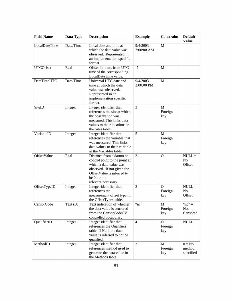
81
Field Name Data Type Description Example Constraint Default Value
LocalDateTime Date/Time Local date and time at which the data value was observed. Represented in an implementation specific format.
9/4/2003 7:00:00 AM
M
UTCOffset Real Offset in hours from UTC time of the corresponding LocalDateTime value.
-7 M
DateTimeUTC Date/Time Universal UTC date and time at which the data value was observed. Represented in an implementation specific format.
9/4/2003 2:00:00 PM
M
SiteID Integer Integer identifier that references the site at which the observation was measured. This links data values to their locations in the Sites table.
3 M Foreign key
VariableID Integer Integer identifier that references the variable that was measured. This links data values to their variable in the Variables table.
5 M Foreign key
OffsetValue Real Distance from a datum or control point to the point at which a data value was observed. If not given the OffsetValue is inferred to be 0, or not relevant/necessary.
2.1 O NULL = No Offset
OffsetTypeID Integer Integer identifier that references the measurement offset type in the OffsetTypes table.
3 O Foreign key
NULL = No Offset
CensorCode Text (50) Text indication of whether the data value is censored from the CensorCodeCV controlled vocabulary.
“nc” M Foreign key
“nc” = Not Censored
QualifierID Integer Integer identifier that references the Qualifiers table. If Null, the data value is inferred to not be qualified.
4 O Foreign key
NULL
MethodID Integer Integer identifier that references method used to generate the data value in the Methods table.
3 M Foreign key
0 = No method specified

82
Field Name Data Type Description Example Constraint Default Value
SourceID Integer Integer identifier that references the record in the Sources table giving the source of the data value.
5 M Foreign key
SampleID Integer Integer identifier that references into the Samples table. This is required only if the data value resulted from a physical sample processed in a lab.
7 O Foreign key
NULL
DerivedFromID Integer Integer identifier for the derived from group of data values that the current data value is derived from. This refers to a group of derived from records in the DerivedFrom table. If NULL, the data value is inferred to not be derived from another data value.
5 O NULL
QualityControlLevelID
Integer Integer identifier giving the level of quality control that the value has been subjected to. This references the QualityControlLevels table.
1 M Foreign key
-9999 = Unknown
The following rules and best practices should be used in populating this table:
1. ValueID is the primary key, is mandatory, and cannot be NULL. This field should be implemented as an autonumber/identity field. When data values are added to this table, a unique integer ValueID should be assigned to each data value by the database software such that the primary key constraint is not violated.
2. Each record in this table must be unique. This is enforced by a unique constraint across all of the fields in this table (excluding ValueID) so that duplicate records are avoided.
3. The LocalDateTime, UTCOffset, and DateTimeUTC must all be populated. Care must be taken to ensure that the correct UTCOffset is used, especially in areas that observe daylight saving time. If LocalDateTime and DateTimeUTC are given, the UTCOffset can be calculated as the difference between the two dates. If LocalDateTime and UTCOffset are given, DateTimeUTC can be calculated.
4. SiteID must correspond to a valid SiteID from the Sites table. When adding data for a new site to the ODM, the Sites table should be populated prior to adding data values to the DataValues table.

83
5. VariableID must correspond to a valid VariableID from the Variables table. When adding data for a new variable to the ODM, the Variables table should be populated prior to adding data values for the new variable to the DataValues table.
6. OffsetValue and OffsetTypeID are optional because not all data values have an offset. Where no offset is used, both of these fields should be set to NULL indicating that the data values do not have an offset. Where an OffsetValue is specified, an OffsetTypeID must also be specified and it must refer to a valid OffsetTypeID in the OffsetTypes table. The OffsetTypes table should be populated prior to adding data values with a particular OffsetTypeID to the DataValues table.
7. CensorCode is mandatory and cannot be NULL. A default value of “nc” is used for this field. Only Terms from the CensorCodeCV table should be used to populate this field.
8. The QualifierID field is optional because not all data values have qualifiers. Where no qualifier applies, this field should be set to NULL. When a QualifierID is specified in this field it must refer to a valid QualifierID in the Qualifiers table. The Qualifiers table should be populated prior to adding data values with a particular QualifierID to the DataValues Table.
9. MethodID must correspond to a valid MethodID from the Methods table and cannot be NULL. A default value of 0 is used in the case where no method is specified or the method used to create the observation is unknown. The Methods table should be populated prior to adding data values with a particular MethodID to the DataValues table.
10. SourceID must correspond to a valid SourceID from the Sources table and cannot be NULL. The Sources table should be populated prior to adding data values with a particular SourceID to the DataValues table.
11. SampleID is optional and should only be populated if the data value was generated from a physical sample that was sent to a laboratory for analysis. The SampleID must correspond to a valid SampleID in the Samples table, and the Samples table should be populated prior to adding data values with a particular SampleID to the DataValues table.
12. DerivedFromID is optional and should only be populated if the data value was derived from other data values that are also stored in the ODM database.
13. QualityControlLevelID is mandatory, cannot be NULL, and must correspond to a valid QualityControlLevelID in the QualityControlLevels table. A default value of -9999 is used for this field in the event that the QualityControlLevelID is unknown. The QualityControlLevels table should be populated prior to adding data values with a particular QualityControlLevelID to the DataValues table.
Table: DerivedFrom The DerivedFrom table contains the linkage between derived data values and the data values that they were derived from.
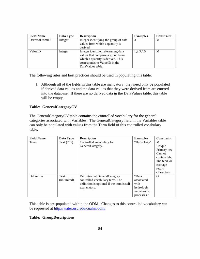
84
Field Name Data Type Description Examples Constraint DerivedFromID Integer Integer identifying the group of data
values from which a quantity is derived.
3 M
ValueID Integer Integer identifier referencing data values that comprise a group from which a quantity is derived. This corresponds to ValueID in the DataValues table.
1,2,3,4,5 M
The following rules and best practices should be used in populating this table:
1. Although all of the fields in this table are mandatory, they need only be populated if derived data values and the data values that they were derived from are entered into the database. If there are no derived data in the DataValues table, this table will be empty.
Table: GeneralCategoryCV The GeneralCategoryCV table contains the controlled vocabulary for the general categories associated with Variables. The GeneralCategory field in the Variables table can only be populated with values from the Term field of this controlled vocabulary table. Field Name Data Type Description Examples Constraint Term Text (255) Controlled vocabulary for
GeneralCategory. “Hydrology” M
Unique Primary key Cannot contain tab, line feed, or carriage return characters
Definition Text (unlimited)
Definition of GeneralCategory controlled vocabulary term. The definition is optional if the term is self explanatory.
“Data associated with hydrologic variables or processes.”
O
This table is pre-populated within the ODM. Changes to this controlled vocabulary can be requested at http://water.usu.edu/cuahsi/odm/. Table: GroupDescriptions

85
The GroupDescriptions table lists the descriptions for each of the groups of data values that have been formed. Field Name Data Type Description Example Constraint GroupID Integer
Identity Unique integer identifier for each group of data values that has been formed. This also references to GroupID in the Groups table.
4 M Unique Primary key
GroupDescription Text (unlimited)
Text description of the group. “Echo Reservoir Profile 7/7/2005”
O
The following rules and best practices should be used in populating this table:
1. This table will only be populated if groups of data values have been created in the ODM database.
2. The GroupID field is the primary key, must be a unique integer, and cannot be NULL. It should be implemented as an auto number/identity field.
3. The GroupDescription can be any text string that describes the group of observations.
Table: Groups The Groups table lists the groups of data values that have been created and the data values that are within each group. Field Name Data Type Description Example Constraint GroupID Integer Integer ID for each
group of data values that has been formed.
4 M Foreign key
ValueID Integer Integer identifier for each data value that belongs to a group. This corresponds to ValueID in the DataValues table
2,3,4 M Foreign key
The following rules and best practices should be used in populating this table:
1. This table will only be populated if groups of data values have been created in the ODM database.
2. The GroupID field must reference a valid GroupID from the GroupDescriptions table, and the GroupDescriptions table should be populated for a group prior to populating the Groups table.
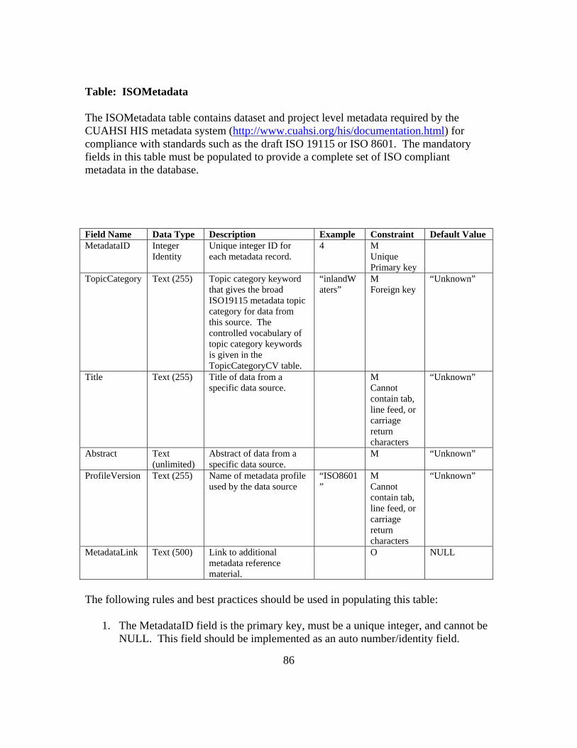
86
Table: ISOMetadata The ISOMetadata table contains dataset and project level metadata required by the CUAHSI HIS metadata system (http://www.cuahsi.org/his/documentation.html) for compliance with standards such as the draft ISO 19115 or ISO 8601. The mandatory fields in this table must be populated to provide a complete set of ISO compliant metadata in the database. Field Name Data Type Description Example Constraint Default Value MetadataID Integer
Identity Unique integer ID for each metadata record.
4 M Unique Primary key
TopicCategory Text (255) Topic category keyword that gives the broad ISO19115 metadata topic category for data from this source. The controlled vocabulary of topic category keywords is given in the TopicCategoryCV table.
“inlandWaters”
M Foreign key
“Unknown”
Title Text (255) Title of data from a specific data source.
M Cannot contain tab, line feed, or carriage return characters
“Unknown”
Abstract Text (unlimited)
Abstract of data from a specific data source.
M “Unknown”
ProfileVersion Text (255) Name of metadata profile used by the data source
“ISO8601”
M Cannot contain tab, line feed, or carriage return characters
“Unknown”
MetadataLink Text (500) Link to additional metadata reference material.
O NULL
The following rules and best practices should be used in populating this table:
1. The MetadataID field is the primary key, must be a unique integer, and cannot be NULL. This field should be implemented as an auto number/identity field.
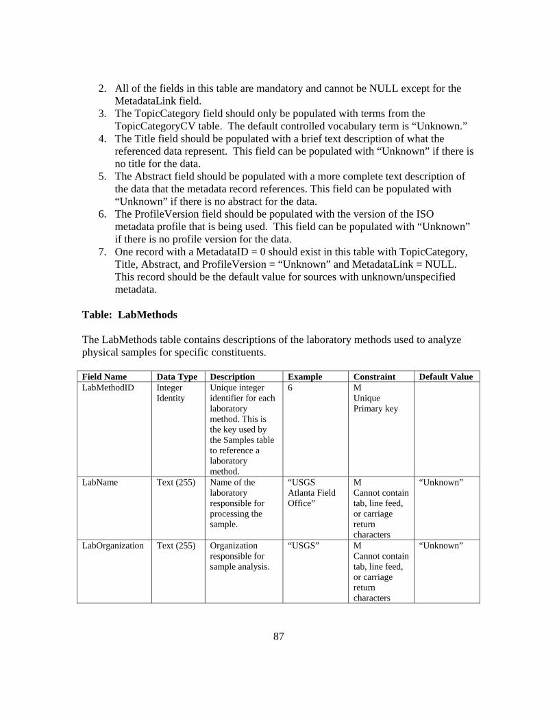
87
2. All of the fields in this table are mandatory and cannot be NULL except for the MetadataLink field.
3. The TopicCategory field should only be populated with terms from the TopicCategoryCV table. The default controlled vocabulary term is “Unknown.”
4. The Title field should be populated with a brief text description of what the referenced data represent. This field can be populated with “Unknown” if there is no title for the data.
5. The Abstract field should be populated with a more complete text description of the data that the metadata record references. This field can be populated with “Unknown” if there is no abstract for the data.
6. The ProfileVersion field should be populated with the version of the ISO metadata profile that is being used. This field can be populated with “Unknown” if there is no profile version for the data.
7. One record with a MetadataID = 0 should exist in this table with TopicCategory, Title, Abstract, and ProfileVersion = “Unknown” and MetadataLink = NULL. This record should be the default value for sources with unknown/unspecified metadata.
Table: LabMethods The LabMethods table contains descriptions of the laboratory methods used to analyze physical samples for specific constituents. Field Name Data Type Description Example Constraint Default Value LabMethodID Integer
Identity Unique integer identifier for each laboratory method. This is the key used by the Samples table to reference a laboratory method.
6 M Unique Primary key
LabName Text (255) Name of the laboratory responsible for processing the sample.
“USGS Atlanta Field Office”
M Cannot contain tab, line feed, or carriage return characters
“Unknown”
LabOrganization Text (255) Organization responsible for sample analysis.
“USGS” M Cannot contain tab, line feed, or carriage return characters
“Unknown”
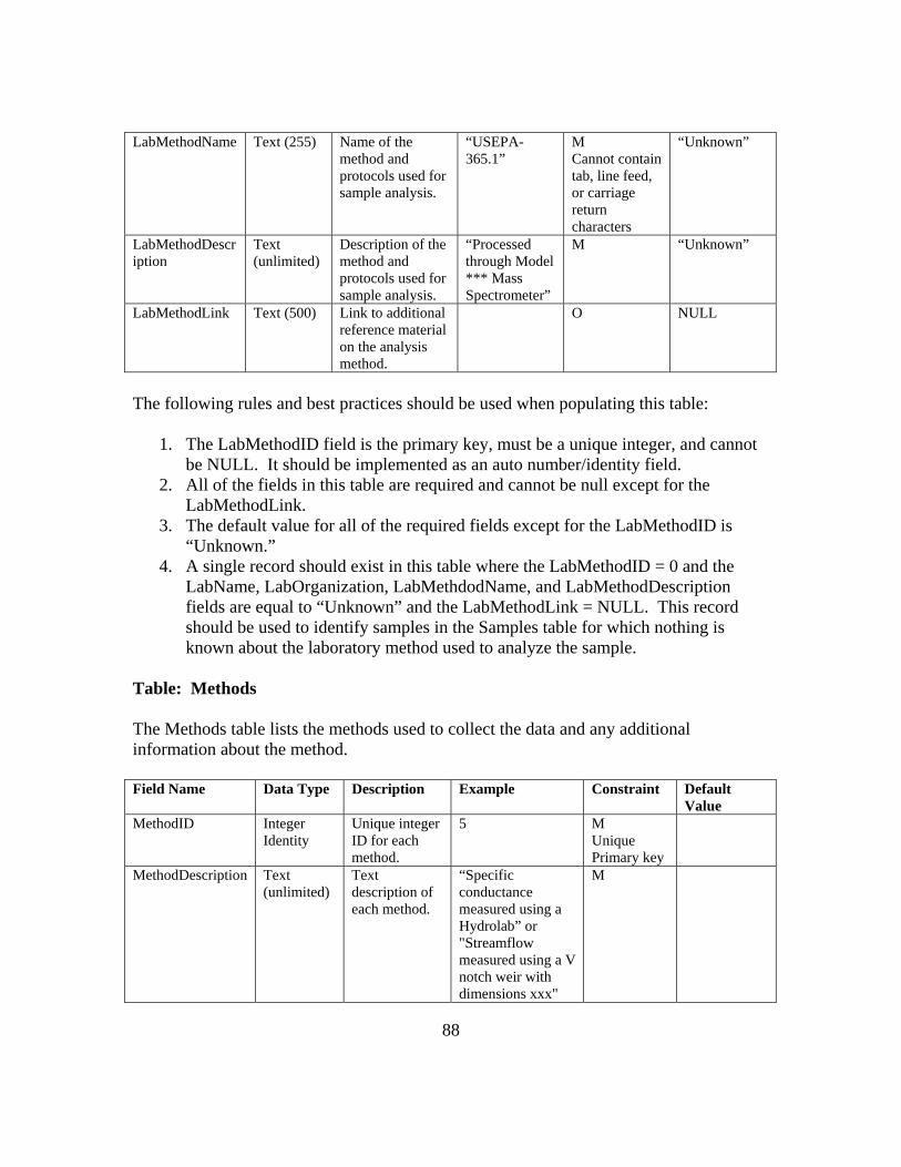
88
LabMethodName Text (255) Name of the method and protocols used for sample analysis.
“USEPA-365.1”
M Cannot contain tab, line feed, or carriage return characters
“Unknown”
LabMethodDescription
Text (unlimited)
Description of the method and protocols used for sample analysis.
“Processed through Model *** Mass Spectrometer”
M “Unknown”
LabMethodLink Text (500) Link to additional reference material on the analysis method.
O NULL
The following rules and best practices should be used when populating this table:
1. The LabMethodID field is the primary key, must be a unique integer, and cannot be NULL. It should be implemented as an auto number/identity field.
2. All of the fields in this table are required and cannot be null except for the LabMethodLink.
3. The default value for all of the required fields except for the LabMethodID is “Unknown.”
4. A single record should exist in this table where the LabMethodID = 0 and the LabName, LabOrganization, LabMethdodName, and LabMethodDescription fields are equal to “Unknown” and the LabMethodLink = NULL. This record should be used to identify samples in the Samples table for which nothing is known about the laboratory method used to analyze the sample.
Table: Methods The Methods table lists the methods used to collect the data and any additional information about the method. Field Name Data Type Description Example Constraint Default
Value MethodID Integer
Identity Unique integer ID for each method.
5 M Unique Primary key
MethodDescription Text (unlimited)
Text description of each method.
“Specific conductance measured using a Hydrolab” or "Streamflow measured using a V notch weir with dimensions xxx"
M
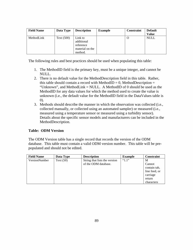
89
Field Name Data Type Description Example Constraint Default Value
MethodLink Text (500) Link to additional reference material on the method.
O NULL
The following rules and best practices should be used when populating this table:
1. The MethodID field is the primary key, must be a unique integer, and cannot be NULL.
2. There is no default value for the MethodDescription field in this table. Rather, this table should contain a record with MethodID = 0, MethodDescription = “Unknown”, and MethodLink = NULL. A MethodID of 0 should be used as the MethodID for any data values for which the method used to create the value is unknown (i.e., the default value for the MethodID field in the DataValues table is 0).
3. Methods should describe the manner in which the observation was collected (i.e., collected manually, or collected using an automated sampler) or measured (i.e., measured using a temperature sensor or measured using a turbidity sensor). Details about the specific sensor models and manufacturers can be included in the MethodDescription.
Table: ODM Version The ODM Version table has a single record that records the version of the ODM database. This table must contain a valid ODM version number. This table will be pre-populated and should not be edited. Field Name Data Type Description Example Constraint VersionNumber Text (50) String that lists the version
of the ODM database. “1.1” M
Cannot contain tab, line feed, or carriage return characters
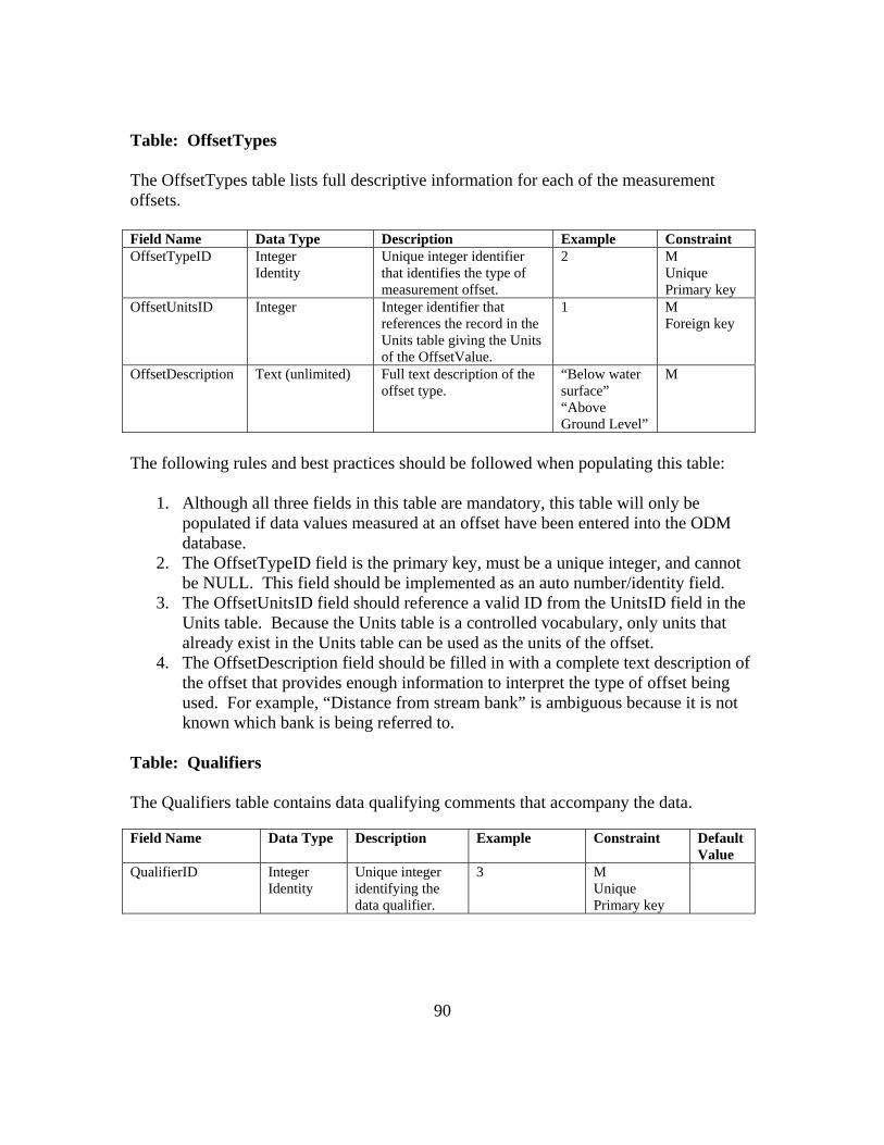
90
Table: OffsetTypes The OffsetTypes table lists full descriptive information for each of the measurement offsets. Field Name Data Type Description Example Constraint OffsetTypeID Integer
Identity Unique integer identifier that identifies the type of measurement offset.
2 M Unique Primary key
OffsetUnitsID Integer Integer identifier that references the record in the Units table giving the Units of the OffsetValue.
1 M Foreign key
OffsetDescription Text (unlimited) Full text description of the offset type.
“Below water surface” “Above Ground Level”
M
The following rules and best practices should be followed when populating this table:
1. Although all three fields in this table are mandatory, this table will only be populated if data values measured at an offset have been entered into the ODM database.
2. The OffsetTypeID field is the primary key, must be a unique integer, and cannot be NULL. This field should be implemented as an auto number/identity field.
3. The OffsetUnitsID field should reference a valid ID from the UnitsID field in the Units table. Because the Units table is a controlled vocabulary, only units that already exist in the Units table can be used as the units of the offset.
4. The OffsetDescription field should be filled in with a complete text description of the offset that provides enough information to interpret the type of offset being used. For example, “Distance from stream bank” is ambiguous because it is not known which bank is being referred to.
Table: Qualifiers The Qualifiers table contains data qualifying comments that accompany the data. Field Name Data Type Description Example Constraint Default
Value QualifierID Integer
Identity Unique integer identifying the data qualifier.
3 M Unique Primary key

91
QualifierCode Text (50) Text code used by organization that collects the data.
“e” (for estimated) or “a” (for approved) or “p” (for provisional)
O Cannot contain space, tab, line feed, or carriage return characters
NULL
QualifierDescription Text (unlimited)
Text of the data qualifying comment.
“Holding time for sample analysis exceeded”
M
This table will only be populated if data values that have data qualifying comments have been added to the ODM database. The following rules and best practices should be used when populating this table:
1. The QualifierID field is the primary key, must be a unique integer, and cannot be NULL. This field should be implemented as an auto number/identity field.
Table: QualityControlLevels The QualityControlLevels table contains the quality control levels that are used for versioning data within the database. Field Name Data Type Description Example Constraint QualityControlLevelID Integer
Identity Unique integer identifying the quality control level.
0, 1, 2, 3, 4, 5 M Unique Primary key
QualityControlLevelCode Text (50) Code used to identify the level of quality control to which data values have been subjected.
“1”, “1.1”, “Raw”, “QC Checked”
M Cannot contain tab, line feed, or carriage return characters
Definition Text (255) Definition of Quality Control Level.
“Raw Data”, “Quality Controlled Data”
M Cannot contain tab, line feed, or carriage return characters
Explanation Text (unlimited)
Explanation of Quality Control Level
“Raw data is defined as unprocessed data and data products that have not undergone quality control.”
M
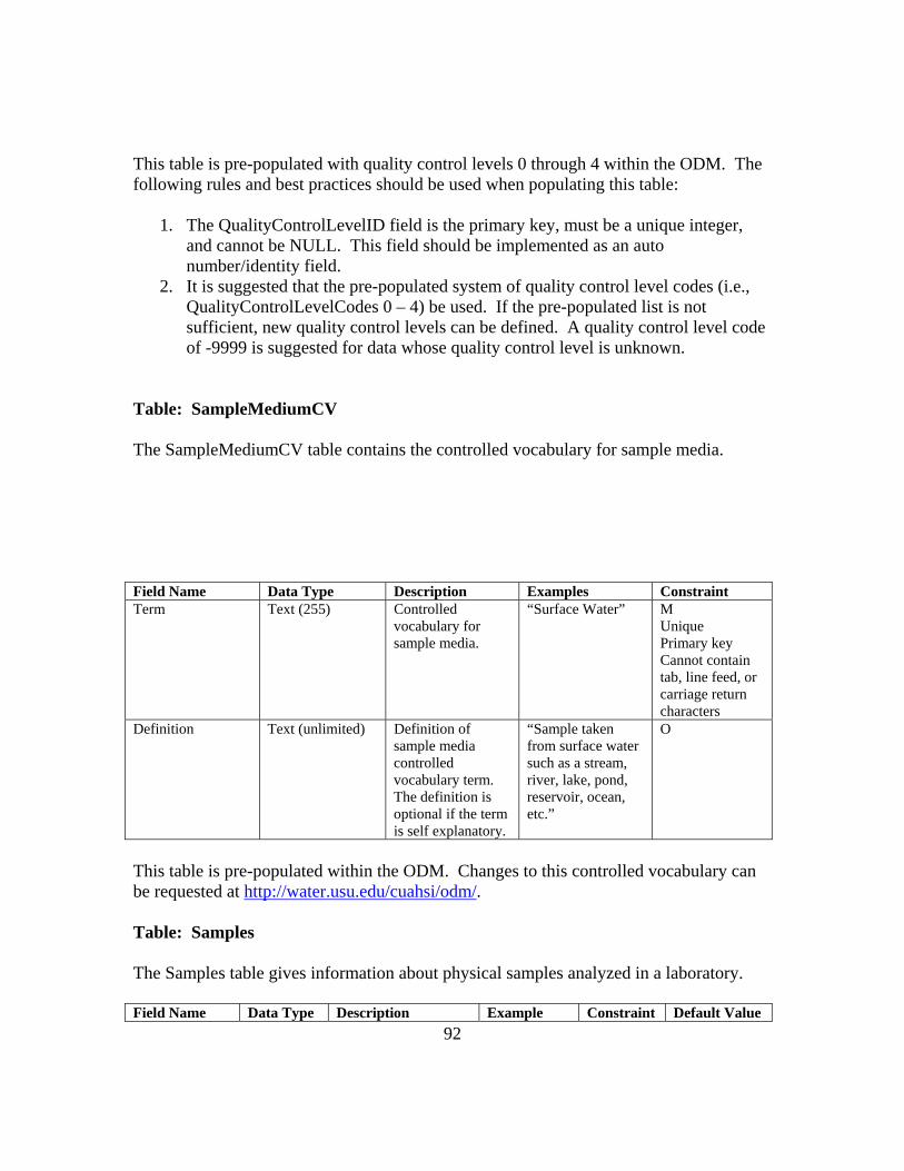
92
This table is pre-populated with quality control levels 0 through 4 within the ODM. The following rules and best practices should be used when populating this table:
1. The QualityControlLevelID field is the primary key, must be a unique integer, and cannot be NULL. This field should be implemented as an auto number/identity field.
2. It is suggested that the pre-populated system of quality control level codes (i.e., QualityControlLevelCodes 0 – 4) be used. If the pre-populated list is not sufficient, new quality control levels can be defined. A quality control level code of -9999 is suggested for data whose quality control level is unknown.
Table: SampleMediumCV The SampleMediumCV table contains the controlled vocabulary for sample media. Field Name Data Type Description Examples Constraint Term Text (255) Controlled
vocabulary for sample media.
“Surface Water” M Unique Primary key Cannot contain tab, line feed, or carriage return characters
Definition Text (unlimited) Definition of sample media controlled vocabulary term. The definition is optional if the term is self explanatory.
“Sample taken from surface water such as a stream, river, lake, pond, reservoir, ocean, etc.”
O
This table is pre-populated within the ODM. Changes to this controlled vocabulary can be requested at http://water.usu.edu/cuahsi/odm/. Table: Samples The Samples table gives information about physical samples analyzed in a laboratory. Field Name Data Type Description Example Constraint Default Value

93
Field Name Data Type Description Example Constraint Default Value SampleID Integer
Identity Unique integer identifier that identifies each physical sample.
3 M Unique Primary key
SampleType Text (255) Controlled vocabulary specifying the sample type from the SampleTypeCV table.
“FD”, “PB”, “SW”, “Grab Sample”
M Foreign key
“Unknown”
LabSampleCode Text (50) Code or label used to identify and track lab sample or sample container (e.g. bottle) during lab analysis.
“AB-123” M Unique Cannot contain tab, line feed, or carriage return characters
LabMethodID Integer Unique identifier for the laboratory method used to process the sample. This references the LabMethods table.
4 M Foreign key
0 = Nothing known about lab method
The following rules and best practices should be followed when populating this table:
1. This table will only be populated if data values associated with physical samples are added to the ODM database.
2. The SamplID field is the primary key, must be a unique integer, and cannot be NULL. This field should be implemented as an auto number/identity field.
3. The SampleType field should be populated using terms from the SampleTypeCV table. Where the sample type is unknown, a default value of “Unknown” can be used.
4. The LabSampleCode should be a unique text code used by the laboratory to identify the sample. This field is an alternate key for this table and should be unique.
5. The LabMethodID must reference a valid LabMethodID from the LabMethods table. The LabMethods table should be populated with the appropriate laboratory method information prior to adding records to this table that reference that laboratory method. A default value of 0 for this field indicates that nothing is known about the laboratory method used to analyze the sample.
Table: SampleTypeCV The SampleTypeCV table contains the controlled vocabulary for sample type. Field Name Data Type Description Examples Constraint
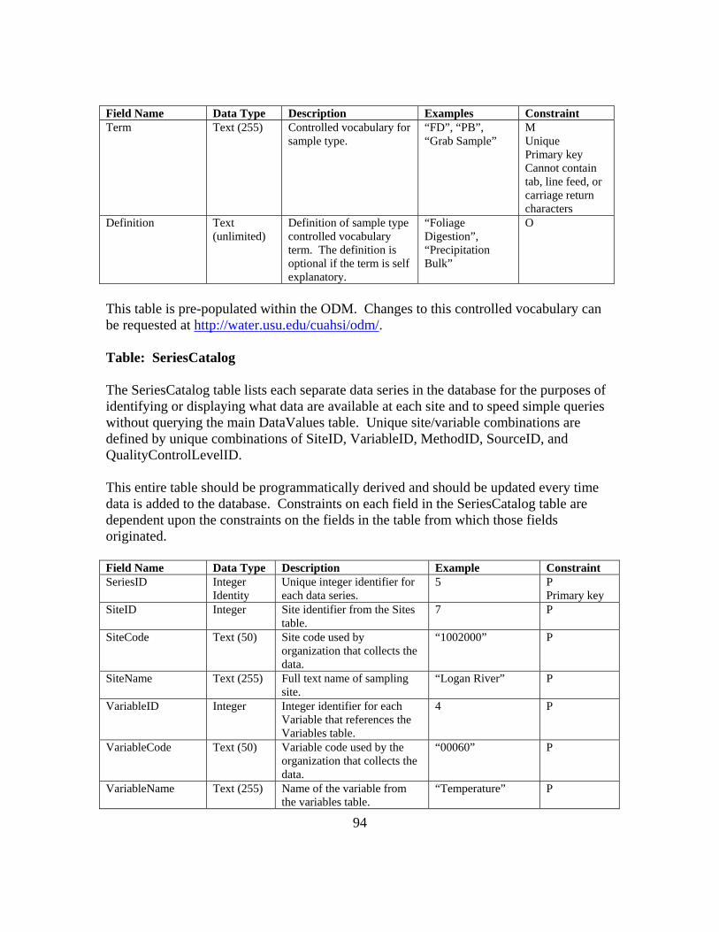
94
Field Name Data Type Description Examples Constraint Term Text (255) Controlled vocabulary for
sample type. “FD”, “PB”, “Grab Sample”
M Unique Primary key Cannot contain tab, line feed, or carriage return characters
Definition Text (unlimited)
Definition of sample type controlled vocabulary term. The definition is optional if the term is self explanatory.
“Foliage Digestion”, “Precipitation Bulk”
O
This table is pre-populated within the ODM. Changes to this controlled vocabulary can be requested at http://water.usu.edu/cuahsi/odm/. Table: SeriesCatalog The SeriesCatalog table lists each separate data series in the database for the purposes of identifying or displaying what data are available at each site and to speed simple queries without querying the main DataValues table. Unique site/variable combinations are defined by unique combinations of SiteID, VariableID, MethodID, SourceID, and QualityControlLevelID. This entire table should be programmatically derived and should be updated every time data is added to the database. Constraints on each field in the SeriesCatalog table are dependent upon the constraints on the fields in the table from which those fields originated. Field Name Data Type Description Example Constraint SeriesID Integer
Identity Unique integer identifier for each data series.
5 P Primary key
SiteID Integer Site identifier from the Sites table.
7 P
SiteCode Text (50) Site code used by organization that collects the data.
“1002000” P
SiteName Text (255) Full text name of sampling site.
“Logan River” P
VariableID Integer Integer identifier for each Variable that references the Variables table.
4 P
VariableCode Text (50) Variable code used by the organization that collects the data.
“00060” P
VariableName Text (255) Name of the variable from the variables table.
“Temperature” P

95
Field Name Data Type Description Example Constraint Speciation Text (255) Code used to identify how
the data value is expressed (i.e., total phosphorus concentration expressed as P). This should be from the SpeciationCV controlled vocabulary table.
“P”, “N”, “NO3” P
VariableUnitsID Integer Integer identifier that references the record in the Units table giving the Units of the data value.
5 P
VariableUnitsName Text (255) Full text name of the variable units from the UnitsName field in the Units table.
“milligrams per liter”
P
SampleMedium Text (255) The medium of the sample. This should be from the SampleMediumCV controlled vocabulary table.
“Surface Water” P
ValueType Text (255) Text value indicating what type of data value is being recorded. This should be from the ValueTypeCV controlled vocabulary table.
“Field Observation” P
TimeSupport Real Numerical value that indicates the time support (or temporal footprint) of the data values. 0 is used to indicate data values that are instantaneous. Other values indicate the time over which the data values are implicitly or explicitly averaged or aggregated.
0, 24 P
TimeUnitsID Integer Integer identifier that references the record in the Units table giving the Units of the time support. If TimeSupport is 0, indicating an instantaneous observation, a unit needs to still be given for completeness, although it is somewhat arbitrary.
4 P
TimeUnitsName Text (255) Full text name of the time support units from the UnitsName field in the Units table.
“hours” P

96
Field Name Data Type Description Example Constraint DataType Text (255) Text value that identifies the
data as one of several types from the DataTypeCV controlled vocabulary table.
“Continuous” “Instantaneous” “Cumulative” “Incremental” “Average” “Minimum” “Maximum” “Constant Over Interval” “Categorical”
P
GeneralCategory Text (255) General category of the variable from the GeneralCategoryCV table.
“Water Quality” P
MethodID Integer Integer identifier that identifies the method used to generate the data values and references the Methods table.
2 P
MethodDescription Text (unlimited)
Full text description of the method used to generate the data values.
“Specific conductance measured using a Hydrolab” or "Streamflow measured using a V notch weir with dimensions xxx"
P
SourceID Integer Integer identifier that identifies the source of the data values and references the Sources table.
5 P
Organization Text (255) Text description of the source organization from the Sources table.
“USGS” P
SourceDescription Text (unlimited)
Text description of the data source from the Sources table.
“Text file retrieved from the EPA STORET system indicating data originally from Utah Division of Water Quality”
P
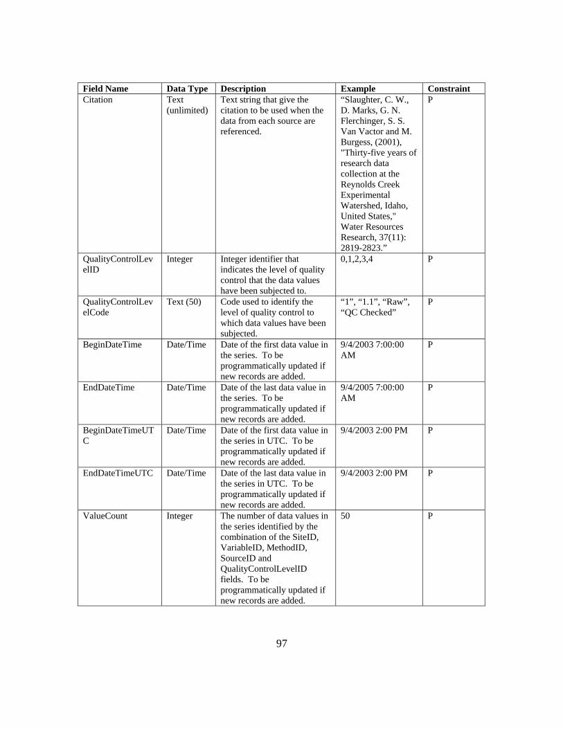
97
Field Name Data Type Description Example Constraint Citation Text
(unlimited) Text string that give the citation to be used when the data from each source are referenced.
“Slaughter, C. W., D. Marks, G. N. Flerchinger, S. S. Van Vactor and M. Burgess, (2001), "Thirty-five years of research data collection at the Reynolds Creek Experimental Watershed, Idaho, United States," Water Resources Research, 37(11): 2819-2823.”
P
QualityControlLevelID
Integer Integer identifier that indicates the level of quality control that the data values have been subjected to.
0,1,2,3,4 P
QualityControlLevelCode
Text (50) Code used to identify the level of quality control to which data values have been subjected.
“1”, “1.1”, “Raw”, “QC Checked”
P
BeginDateTime Date/Time Date of the first data value in the series. To be programmatically updated if new records are added.
9/4/2003 7:00:00 AM
P
EndDateTime Date/Time Date of the last data value in the series. To be programmatically updated if new records are added.
9/4/2005 7:00:00 AM
P
BeginDateTimeUTC
Date/Time Date of the first data value in the series in UTC. To be programmatically updated if new records are added.
9/4/2003 2:00 PM P
EndDateTimeUTC Date/Time Date of the last data value in the series in UTC. To be programmatically updated if new records are added.
9/4/2003 2:00 PM P
ValueCount Integer The number of data values in the series identified by the combination of the SiteID, VariableID, MethodID, SourceID and QualityControlLevelID fields. To be programmatically updated if new records are added.
50 P
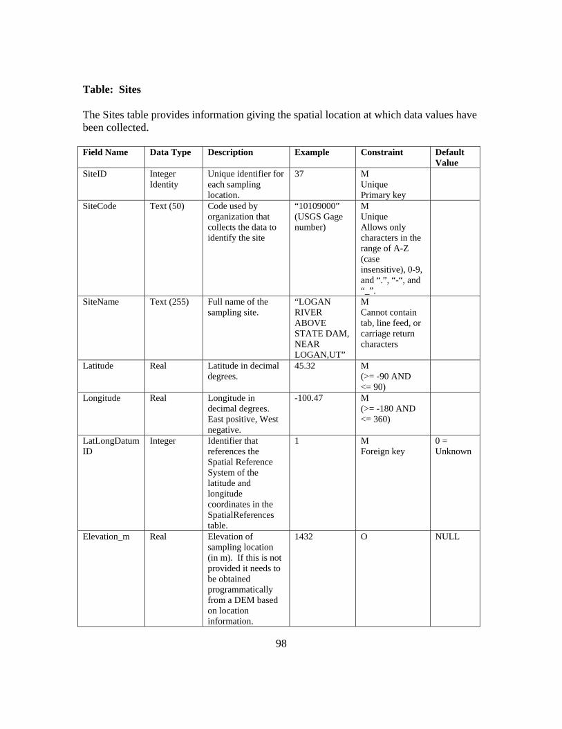
98
Table: Sites The Sites table provides information giving the spatial location at which data values have been collected. Field Name Data Type Description Example Constraint Default
Value SiteID Integer
Identity Unique identifier for each sampling location.
37 M Unique Primary key
SiteCode Text (50) Code used by organization that collects the data to identify the site
“10109000” (USGS Gage number)
M Unique Allows only characters in the range of A-Z (case insensitive), 0-9, and “.”, “-“, and “_”.
SiteName Text (255) Full name of the sampling site.
“LOGAN RIVER ABOVE STATE DAM, NEAR LOGAN,UT”
M Cannot contain tab, line feed, or carriage return characters
Latitude Real Latitude in decimal degrees.
45.32 M (>= -90 AND <= 90)
Longitude Real Longitude in decimal degrees. East positive, West negative.
-100.47 M (>= -180 AND <= 360)
LatLongDatumID
Integer Identifier that references the Spatial Reference System of the latitude and longitude coordinates in the SpatialReferences table.
1 M Foreign key
0 = Unknown
Elevation_m Real Elevation of sampling location (in m). If this is not provided it needs to be obtained programmatically from a DEM based on location information.
1432 O NULL
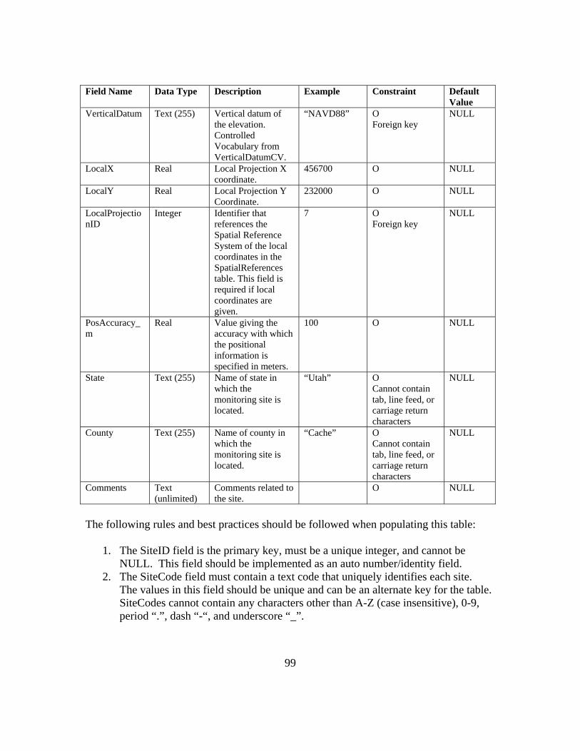
99
Field Name Data Type Description Example Constraint Default Value
VerticalDatum Text (255) Vertical datum of the elevation. Controlled Vocabulary from VerticalDatumCV.
“NAVD88” O Foreign key
NULL
LocalX Real Local Projection X coordinate.
456700 O NULL
LocalY Real Local Projection Y Coordinate.
232000 O NULL
LocalProjectionID
Integer Identifier that references the Spatial Reference System of the local coordinates in the SpatialReferences table. This field is required if local coordinates are given.
7 O Foreign key
NULL
PosAccuracy_m
Real Value giving the accuracy with which the positional information is specified in meters.
100 O NULL
State Text (255) Name of state in which the monitoring site is located.
“Utah” O Cannot contain tab, line feed, or carriage return characters
NULL
County Text (255) Name of county in which the monitoring site is located.
“Cache” O Cannot contain tab, line feed, or carriage return characters
NULL
Comments Text (unlimited)
Comments related to the site.
O NULL
The following rules and best practices should be followed when populating this table:
1. The SiteID field is the primary key, must be a unique integer, and cannot be NULL. This field should be implemented as an auto number/identity field.
2. The SiteCode field must contain a text code that uniquely identifies each site. The values in this field should be unique and can be an alternate key for the table. SiteCodes cannot contain any characters other than A-Z (case insensitive), 0-9, period “.”, dash “-“, and underscore “_”.

100
3. The LatLongDatumID must reference a valid SpatialReferenceID from the SpatialReferences controlled vocabulary table. If the datum is unknown, a default value of 0 is used.
4. If the Elevation_m field is populated with a numeric value, a value must be specified in the VerticalDatum field. The VerticalDatum field can only be populated using terms from the VerticalDatumCV table. If the vertical datum is unknown, a value of “Unknown” is used.
5. If the LocalX and LocalY fields are populated with numeric values, a value must be specified in the LocalProjectionID field. The LocalProjectionID must reference a valid SpatialReferenceID from the SpatialReferences controlled vocabulary table. If the spatial reference system of the local coordinates is unknown, a default value of 0 is used.
Table: Sources The Sources table lists the original sources of the data, providing information sufficient to retrieve and reconstruct the data value from the original data files if necessary. Field Name Data Type Description Example Constraint Default
Value SourceID Integer
Identity Unique integer identifier that identifies each data source.
5 M Unique Primary key
Organization Text (255) Name of the organization that collected the data. This should be the agency or organization that collected the data, even if it came out of a database consolidated from many sources such as STORET.
“Utah Division of Water Quality”
M Cannot contain tab, line feed, or carriage return characters
SourceDescription Text (unlimited)
Full text description of the source of the data.
“Text file retrieved from the EPA STORET system indicating data originally from Utah Division of Water Quality”
M
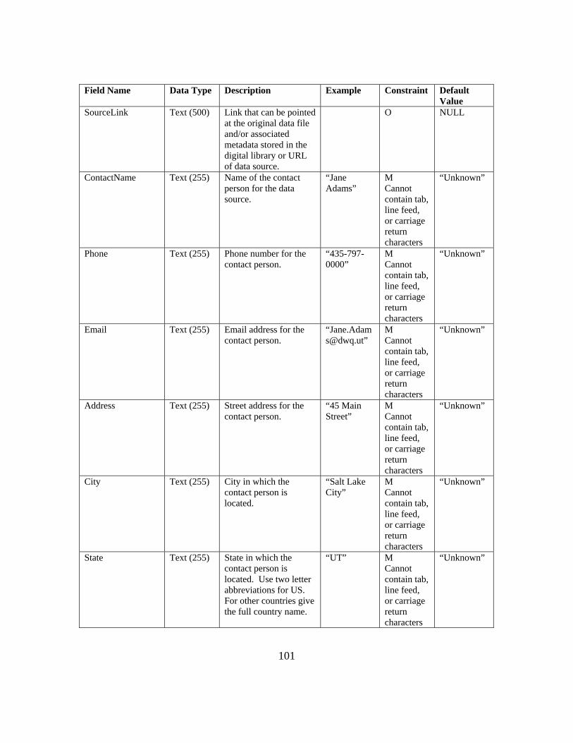
101
Field Name Data Type Description Example Constraint Default Value
SourceLink Text (500) Link that can be pointed at the original data file and/or associated metadata stored in the digital library or URL of data source.
O NULL
ContactName Text (255) Name of the contact person for the data source.
“Jane Adams”
M Cannot contain tab, line feed, or carriage return characters
“Unknown”
Phone Text (255) Phone number for the contact person.
“435-797-0000”
M Cannot contain tab, line feed, or carriage return characters
“Unknown”
Email Text (255) Email address for the contact person.
M Cannot contain tab, line feed, or carriage return characters
“Unknown”
Address Text (255) Street address for the contact person.
“45 Main Street”
M Cannot contain tab, line feed, or carriage return characters
“Unknown”
City Text (255) City in which the contact person is located.
“Salt Lake City”
M Cannot contain tab, line feed, or carriage return characters
“Unknown”
State Text (255) State in which the contact person is located. Use two letter abbreviations for US. For other countries give the full country name.
“UT” M Cannot contain tab, line feed, or carriage return characters
“Unknown”

102
Field Name Data Type Description Example Constraint Default Value
ZipCode Text (255) US Zip Code or country postal code.
“82323” M Cannot contain tab, line feed, or carriage return characters
“Unknown”
Citation Text (unlimited)
Text string that give the citation to be used when the data from each source are referenced.
“Data collected by USU as part of the Little Bear River Test Bed Project”
M “Unknown”
MetadataID Integer Integer identifier referencing the record in the ISOMetadata table for this source.
5 M Foreign key
0 = Unknown or uninitialized metadata
The following rules and best practices should be followed when populating this table:
1. The SourceID field is the primary key, must be a unique integer, and cannot be NULL. This field should be implemented as an auto number/identity field.
2. The Organization field should contain a text description of the agency or organization that created the data.
3. The SourceDescription field should contain a more detailed description of where the data was actually obtained.
4. A default value of “Unknown” may be used for the source contact information fields in the event that this information is not known.
5. Each source must be associated with a metadata record in the ISOMetadata table. As such, the MetadataID must reference a valid MetadataID from the ISOMetadata table. The ISOMetatadata table should be populated with an appropriate record prior to adding a source to the Sources table. A default MetadataID of 0 can be used for a source with unknown or uninitialized metadata.
6. Use the Citation field to record the text that you would like others to use when they are referencing your data. Where available, journal citations are encouraged to promote the correct crediting for use of data.
Table: SpatialReferences The SpatialReferences table provides information about the Spatial Reference Systems used for latitude and longitude as well as local coordinate systems in the Sites table. This table is a controlled vocabulary.
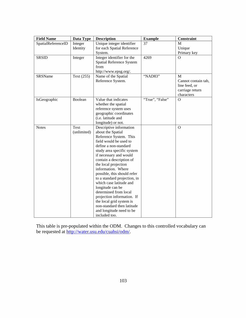
103
Field Name Data Type Description Example Constraint SpatialReferenceID Integer
Identity Unique integer identifier for each Spatial Reference System.
37 M Unique Primary key
SRSID Integer Integer identifier for the Spatial Reference System from http://www.epsg.org/.
4269 O
SRSName Text (255) Name of the Spatial Reference System.
“NAD83” M Cannot contain tab, line feed, or carriage return characters
IsGeographic Boolean Value that indicates whether the spatial reference system uses geographic coordinates (i.e. latitude and longitude) or not.
“True”, “False” O
Notes Text (unlimited)
Descriptive information about the Spatial Reference System. This field would be used to define a non-standard study area specific system if necessary and would contain a description of the local projection information. Where possible, this should refer to a standard projection, in which case latitude and longitude can be determined from local projection information. If the local grid system is non-standard then latitude and longitude need to be included too.
O
This table is pre-populated within the ODM. Changes to this controlled vocabulary can be requested at http://water.usu.edu/cuahsi/odm/.
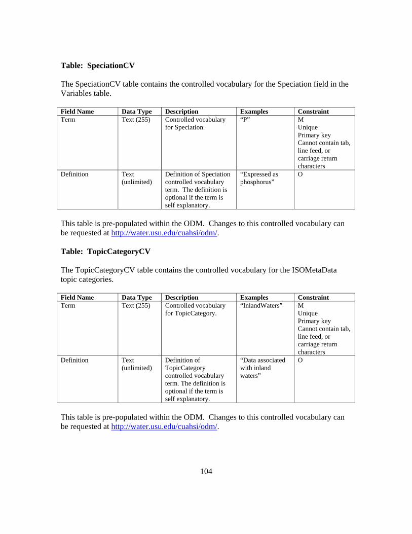
104
Table: SpeciationCV The SpeciationCV table contains the controlled vocabulary for the Speciation field in the Variables table. Field Name Data Type Description Examples Constraint Term Text (255) Controlled vocabulary
for Speciation. “P” M
Unique Primary key Cannot contain tab, line feed, or carriage return characters
Definition Text (unlimited)
Definition of Speciation controlled vocabulary term. The definition is optional if the term is self explanatory.
“Expressed as phosphorus”
O
This table is pre-populated within the ODM. Changes to this controlled vocabulary can be requested at http://water.usu.edu/cuahsi/odm/. Table: TopicCategoryCV The TopicCategoryCV table contains the controlled vocabulary for the ISOMetaData topic categories. Field Name Data Type Description Examples Constraint Term Text (255) Controlled vocabulary
for TopicCategory. “InlandWaters” M
Unique Primary key Cannot contain tab, line feed, or carriage return characters
Definition Text (unlimited)
Definition of TopicCategory controlled vocabulary term. The definition is optional if the term is self explanatory.
“Data associated with inland waters”
O
This table is pre-populated within the ODM. Changes to this controlled vocabulary can be requested at http://water.usu.edu/cuahsi/odm/.
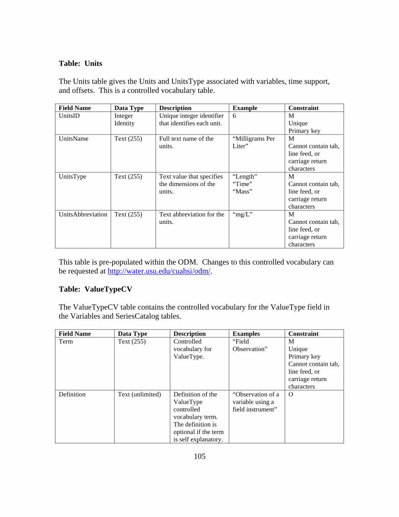
105
Table: Units The Units table gives the Units and UnitsType associated with variables, time support, and offsets. This is a controlled vocabulary table. Field Name Data Type Description Example Constraint UnitsID Integer
Identity Unique integer identifier that identifies each unit.
6 M Unique Primary key
UnitsName Text (255) Full text name of the units.
“Milligrams Per Liter”
M Cannot contain tab, line feed, or carriage return characters
UnitsType Text (255) Text value that specifies the dimensions of the units.
“Length” “Time” “Mass”
M Cannot contain tab, line feed, or carriage return characters
UnitsAbbreviation Text (255) Text abbreviation for the units.
“mg/L” M Cannot contain tab, line feed, or carriage return characters
This table is pre-populated within the ODM. Changes to this controlled vocabulary can be requested at http://water.usu.edu/cuahsi/odm/. Table: ValueTypeCV The ValueTypeCV table contains the controlled vocabulary for the ValueType field in the Variables and SeriesCatalog tables. Field Name Data Type Description Examples Constraint Term Text (255) Controlled
vocabulary for ValueType.
“Field Observation”
M Unique Primary key Cannot contain tab, line feed, or carriage return characters
Definition Text (unlimited) Definition of the ValueType controlled vocabulary term. The definition is optional if the term is self explanatory.
“Observation of a variable using a field instrument”
O

106
This table is pre-populated within the ODM. Changes to this controlled vocabulary can be requested at http://water.usu.edu/cuahsi/odm/. Table: VariableNameCV The VariableName CV table contains the controlled vocabulary for the VariableName field in the Variables and SeriesCatalog tables. Field Name Data Type Description Examples Constraint Term Text (255) Controlled
vocabulary for Variable names.
"Temperature", "Discharge", "Precipitation"
M Unique Primary key Cannot contain tab, line feed, or carriage return characters
Definition Text (unlimited) Definition of the VariableName controlled vocabulary term. The definition is optional if the term is self explanatory.
O
This table is pre-populated within the ODM. Changes to this controlled vocabulary can be requested at http://water.usu.edu/cuahsi/odm/. Table: Variables The Variables table lists the full descriptive information about what variables have been measured. Field Name Data Type Description Example Constraint Default
Value VariableID Integer
Identity Unique integer identifier for each variable.
6 M Unique Primary key
VariableCode Text (50) Text code used by the organization that collects the data to identify the variable.
“00060” used by USGS for discharge
M Unique Allows only characters in the range of A-Z (case insensitive), 0-9, and “.”, “-“, and “_”.
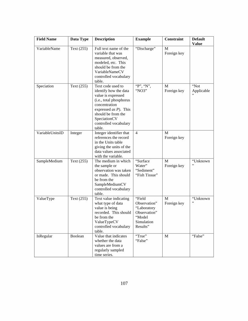
107
Field Name Data Type Description Example Constraint Default Value
VariableName Text (255) Full text name of the variable that was measured, observed, modeled, etc. This should be from the VariableNameCV controlled vocabulary table.
“Discharge” M Foreign key
Speciation Text (255) Text code used to identify how the data value is expressed (i.e., total phosphorus concentration expressed as P). This should be from the SpeciationCV controlled vocabulary table.
“P”, “N”, “NO3”
M Foreign key
“Not Applicable”
VariableUnitsID Integer Integer identifier that references the record in the Units table giving the units of the data values associated with the variable.
4 M Foreign key
SampleMedium Text (255) The medium in which the sample or observation was taken or made. This should be from the SampleMediumCV controlled vocabulary table.
“Surface Water” “Sediment” “Fish Tissue”
M Foreign key
“Unknown”
ValueType Text (255) Text value indicating what type of data value is being recorded. This should be from the ValueTypeCV controlled vocabulary table.
“Field Observation” “Laboratory Observation” “Model Simulation Results”
M Foreign key
“Unknown”
IsRegular Boolean Value that indicates whether the data values are from a regularly sampled time series.
“True” “False”
M “False”

108
Field Name Data Type Description Example Constraint Default Value
TimeSupport Real Numerical value that indicates the time support (or temporal footprint) of the data values. 0 is used to indicate data values that are instantaneous. Other values indicate the time over which the data values are implicitly or explicitly averaged or aggregated.
0, 24 M 0 = Assumes instantaneous samples where no other information is available
TimeUnitsID Integer Integer identifier that references the record in the Units table giving the Units of the time support. If TimeSupport is 0, indicating an instantaneous observation, a unit needs to still be given for completeness, although it is somewhat arbitrary.
4 M Foreign key
103 = hours
DataType Text (255) Text value that identifies the data values as one of several types from the DataTypeCV controlled vocabulary table.
“Continuous” “Sporadic” “Cumulative” “Incremental” “Average” “Minimum” “Maximum” “Constant Over Interval” “Categorical”
M Foreign key
“Unknown”
GeneralCategory Text (255) General category of the data values from the GeneralCategoryCV controlled vocabulary table.
“Climate” “Water Quality” “Groundwater Quality”
M Foreign key
“Unknown”
NoDataValue Real Numeric value used to encode no data values for this variable.
-9999 M -9999
The following rules and best practices should be followed when populating this table:

109
1. The VariableID field is the primary key, must be a unique integer, and cannot be NULL. This field should be implemented as an auto number/identity field.
2. The VariableCode field must be unique and serves as an alternate key for this table. Variable codes can be arbitrary, or they can use an organized system. VaraibleCodes cannot contain any characters other than A-Z (case insensitive), 0-9, period “.”, dash “-“, and underscore “_”.
3. The VariableName field must reference a valid Term from the VariableNameCV controlled vocabulary table.
4. The Speciation field must reference a valid Term from the SpeciationCV controlled vocabulary table. A default value of “Not Applicable” is used where speciation does not apply. If the speciation is unknown, a value of “Unknown” can be used.
5. The VariableUnitsID field must reference a valid UnitsID from the UnitsTable controlled vocabulary table.
6. Only terms from the SampleMediumCV table can be used to populate the SampleMedium field. A default value of “Unknown” is used where the sample medium is unknown.
7. Only terms from the ValueTypeCV table can be used to populate the ValueType field. A default value of “Unknown” is used where the value type is unknown.
8. The default for the TimeSupport field is 0. This corresponds to instantaneous values. If the TimeSupport field is set to a value other than 0, an appropriate TimeUnitsID must be specified. The TimeUnitsID field can only reference valid UnitsID values from the Units controlled vocabulary table. If the TimeSupport field is set to 0, any time units can be used (i.e., seconds, minutes, hours, etc.), however a default value of 103 has been used, which corresponds with hours.
9. Only terms from the DataTypeCV table can be used to populated the DataType field. A default value of “Unknown” can be used where the data type is unknown.
10. Only terms from the GeneralCategoryCV table can be used to populate the GeneralCategory field. A default value of “Unknown” can be used where the general category is unknown.
11. The NoDataValue should be set such that it will never conflict with a real observation value. For example a NoDataValue of -9999 is valid for water temperature because we would never expect to measure a water temperature of -9999. The default value for this field is -9999.
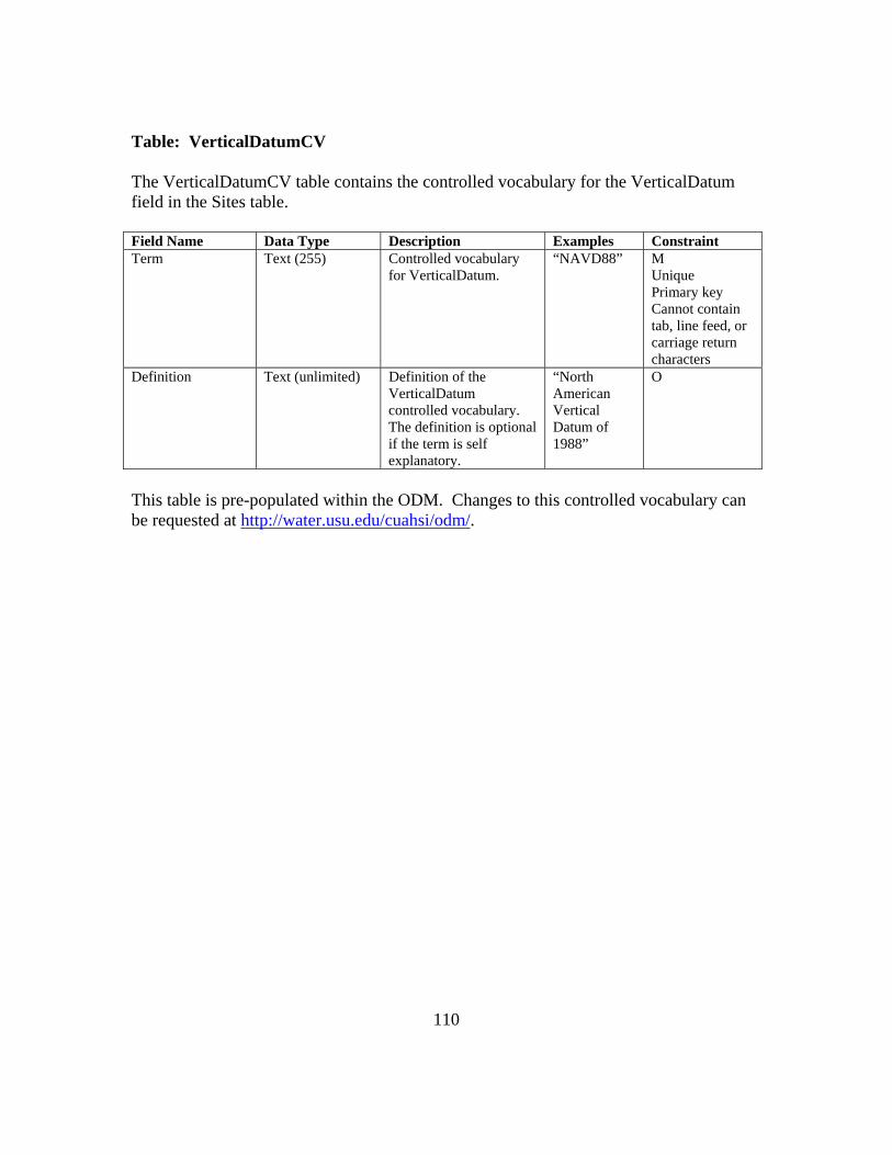
110
Table: VerticalDatumCV The VerticalDatumCV table contains the controlled vocabulary for the VerticalDatum field in the Sites table. Field Name Data Type Description Examples Constraint Term Text (255) Controlled vocabulary
for VerticalDatum. “NAVD88” M
Unique Primary key Cannot contain tab, line feed, or carriage return characters
Definition Text (unlimited) Definition of the VerticalDatum controlled vocabulary. The definition is optional if the term is self explanatory.
“North American Vertical Datum of 1988”
O
This table is pre-populated within the ODM. Changes to this controlled vocabulary can be requested at http://water.usu.edu/cuahsi/odm/.

111
APPENDIX C: SSIS DATA LOADING TUTORIAL
The first step in uploading data through SSIS is to attach an ODM into your SQL Server. Do this by first creating a new file, let’s call it SSIS-Tutorial in the SQLData file on the HIS “O” drive. (O:\SQLData\SSISTutorial). Once created download a blank ODM 1.1 database and log file from the CUAHSI website into this file. Once this is completed the file should appear as this;
Next open SQL Server Management studios from the start menu (Start>Programs>SQL Server 2005>SQL Server Management Studio) and click connect to get past the initial check in. Once in management studios we need to attach our downloaded ODM database within SQL Server. Right click on the databases tab and click “Attach…”.
Click on the “Add” button in the Attach Databases window and navigate to the newly downloaded ODM. Click ok to get back to the Attach Databases window and under “Attach As” click to rename your database to whatever you choose, here I name mine SSISTutorial.

112
Exit out of SQL Server management Studios and open SQL Server Business Intelligence Development Studio and create a new SSIS project. (File>New>Project). Once the new project window is displayed select the Integration Services Project template under the Business Intelligence Services tab, input a project name and browse to where you want to house your SSIS files. Once a project is opened drag and drop a Data Flow Task icon to the Control Flow work area.

113
This Data Flow Task can be renamed for later ease of use by single clicking on the name and typing in the desired name. Double click on the Data Flow Task icon to enter the Data Flow work environment. Drag and drop the Flat File Source icon from the Data Flow Sources toolbox. This allows you to upload documents from a flat file such as a .csv or .txt file.
Open the Flat File Source Editor by double clicking on the icon and chose to create a new connection. Assign a descriptive name, such as Tutorial Site Source and browse to the file you want to upload.
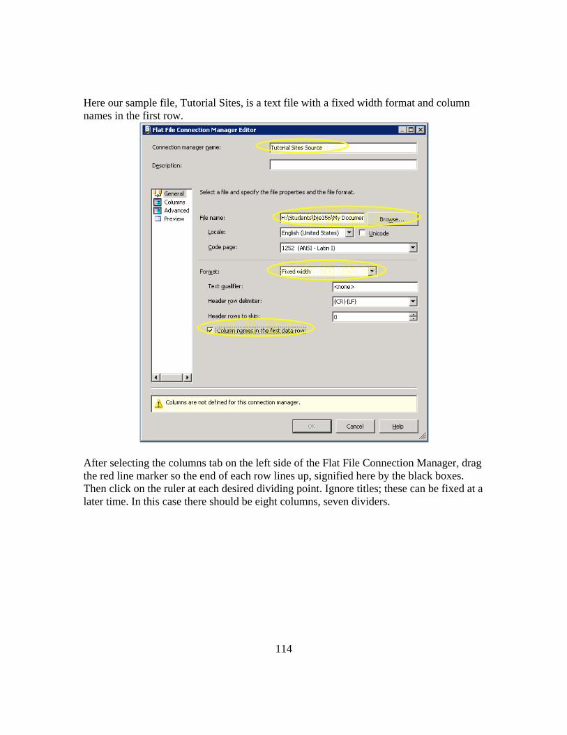
114
Here our sample file, Tutorial Sites, is a text file with a fixed width format and column names in the first row.
After selecting the columns tab on the left side of the Flat File Connection Manager, drag the red line marker so the end of each row lines up, signified here by the black boxes. Then click on the ruler at each desired dividing point. Ignore titles; these can be fixed at a later time. In this case there should be eight columns, seven dividers.

115
Click on the advanced tab to set each column name and rename each site so it can be later identified. Clicking on the current name for the column will allow you to change the name by editing the Name box. After editing you can preview the data or just click OK to save your changes.

116
The next step in this process is data transformation. Drag and drop the Script Component icon and then link the two icons by dragging the green arrow from the Flat File Source icon to the Script Component.
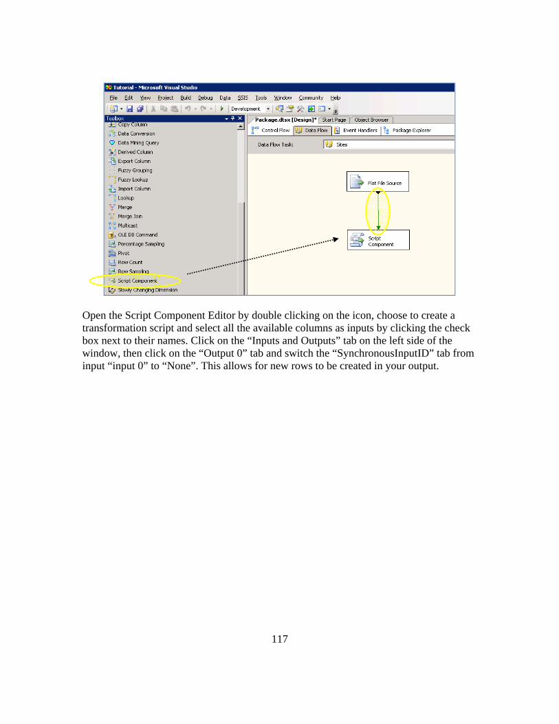
117
Open the Script Component Editor by double clicking on the icon, choose to create a transformation script and select all the available columns as inputs by clicking the check box next to their names. Click on the “Inputs and Outputs” tab on the left side of the window, then click on the “Output 0” tab and switch the “SynchronousInputID” tab from input “input 0” to “None”. This allows for new rows to be created in your output.
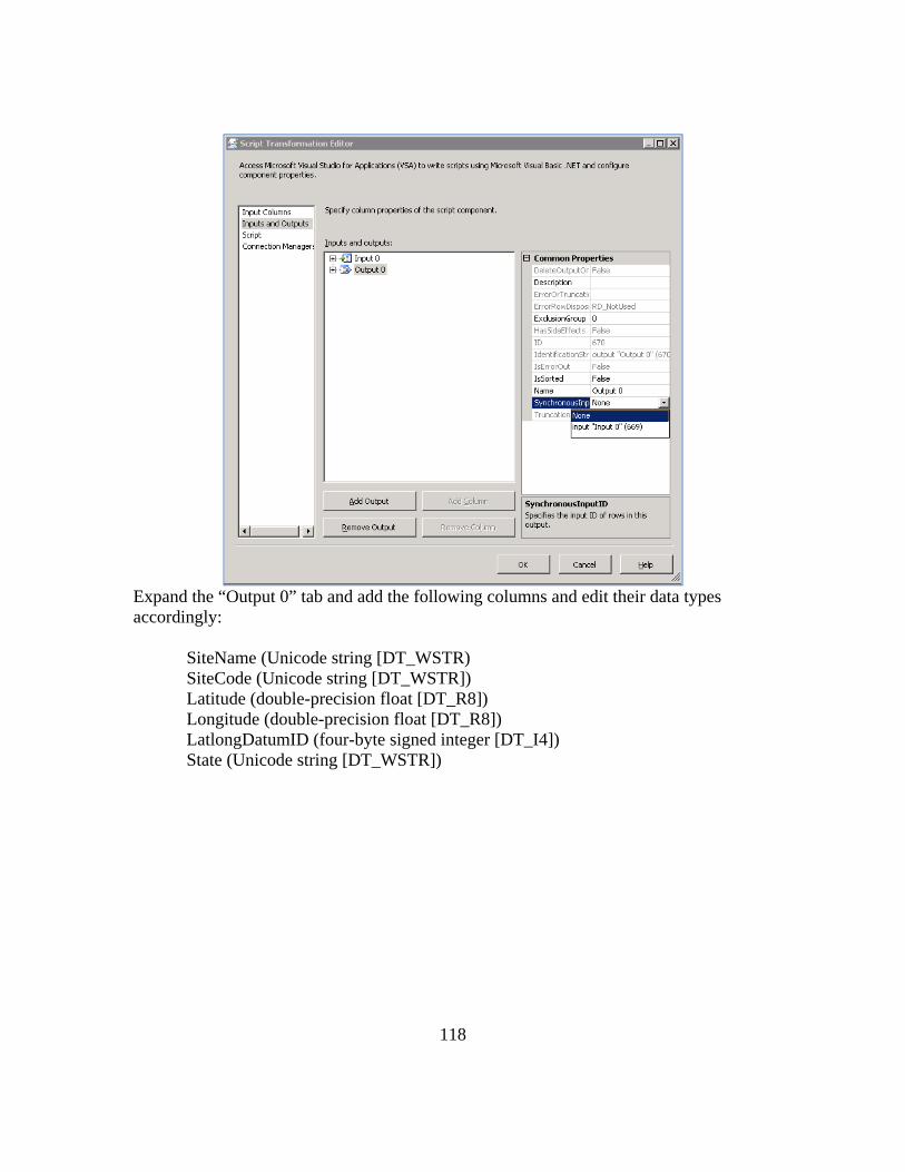
118
Expand the “Output 0” tab and add the following columns and edit their data types accordingly:
SiteName (Unicode string [DT_WSTR) SiteCode (Unicode string [DT_WSTR]) Latitude (double-precision float [DT_R8]) Longitude (double-precision float [DT_R8]) LatlongDatumID (four-byte signed integer [DT_I4]) State (Unicode string [DT_WSTR])
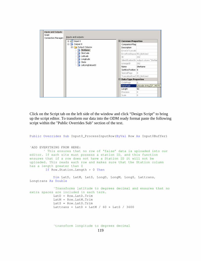
119
Click on the Script tab on the left side of the window and click “Design Script” to bring up the script editor. To transform our data into the ODM ready format paste the following script within the "Public Overrides Sub" section of the text. Public Overrides Sub Input0_ProcessInputRow(ByVal Row As Input0Buffer) 'ADD EVERYTHING FROM HERE: ' This ensures that no row of “false” data is uploaded into our editor. If each site must possess a station ID, and this function ensures that if a row does not have a Station ID it will not be uploaded. This reads each row and makes sure that the Station column has a length greater than 0 If Row.Station.Length > 0 Then Dim LatD, LatM, LatS, LongD, LongM, LongS, Lattrans, Longtrans As Double 'Transforms latitude to degrees decimal and ensures that no extra spaces are included in each term. LatD = Row.LatD.Trim LatM = Row.LatM.Trim LatS = Row.LatS.Trim Lattrans = LatD + LatM / 60 + LatS / 3600 'transform longitude to degrees decimal

120
LongD = Row.LongD.Trim LongM = Row.LongM.Trim LongS = Row.LongS.Trim Longtrans = -(LongD + LongM / 60 + LongS / 3600) 'Create an output table for the ODM .Addrow() allows for the creation of the rows that were stated earlier With Output0Buffer .AddRow() .SiteCode = "Tutorial" & Row.Station.Trim .SiteName = Row.Name.Trim .LatLongDatumID = 2 .Latitude = Lattrans .Longitude = Longtrans .State = "Texas" End With End If 'TO HERE End Sub After entering the Script exit the editor and return to the main screen by clicking ok. Your edits will be saved once ok is clicked. Drag the Flat File Destination icon from toolbar and connect it to the Script Component icon box. This step writes your file to an output file which allows the user to check to ensure that the output is correct before inserting it into the ODM.
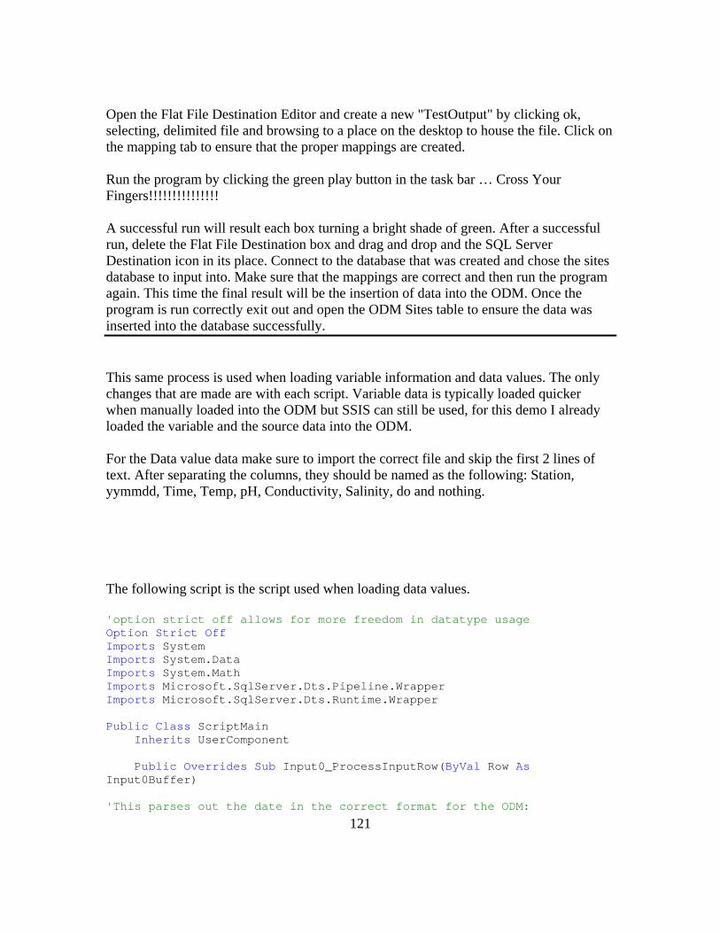
121
Open the Flat File Destination Editor and create a new "TestOutput" by clicking ok, selecting, delimited file and browsing to a place on the desktop to house the file. Click on the mapping tab to ensure that the proper mappings are created. Run the program by clicking the green play button in the task bar … Cross Your Fingers!!!!!!!!!!!!!!! A successful run will result each box turning a bright shade of green. After a successful run, delete the Flat File Destination box and drag and drop and the SQL Server Destination icon in its place. Connect to the database that was created and chose the sites database to input into. Make sure that the mappings are correct and then run the program again. This time the final result will be the insertion of data into the ODM. Once the program is run correctly exit out and open the ODM Sites table to ensure the data was inserted into the database successfully. This same process is used when loading variable information and data values. The only changes that are made are with each script. Variable data is typically loaded quicker when manually loaded into the ODM but SSIS can still be used, for this demo I already loaded the variable and the source data into the ODM. For the Data value data make sure to import the correct file and skip the first 2 lines of text. After separating the columns, they should be named as the following: Station, yymmdd, Time, Temp, pH, Conductivity, Salinity, do and nothing. The following script is the script used when loading data values. 'option strict off allows for more freedom in datatype usage Option Strict Off Imports System Imports System.Data Imports System.Math Imports Microsoft.SqlServer.Dts.Pipeline.Wrapper Imports Microsoft.SqlServer.Dts.Runtime.Wrapper Public Class ScriptMain Inherits UserComponent Public Overrides Sub Input0_ProcessInputRow(ByVal Row As Input0Buffer) 'This parses out the date in the correct format for the ODM:

122
Dim Month, day, year, hour, min As Integer Dim rowDateTime As String Dim AmPm As String Month = Row.yymmdd.Trim.Substring(2, 2) day = Row.yymmdd.Trim.Substring(4, 2) year = Row.yymmdd.Trim.Substring(0, 2) If Row.Time.Trim.Length = 4 Then hour = Row.Time.Trim.Substring(0, 2) If hour > 12 Then hour = hour - 12 AmPm = "pm" Else AmPm = "am" End If If hour = 12 Then AmPm = "pm" min = Row.Time.Trim.Substring(2, 2) ElseIf Row.Time.Trim.Length = 3 Then hour = Row.Time.Trim.Substring(0, 1) If hour > 12 Then hour = hour - 12 AmPm = "pm" Else AmPm = "am" End If If hour = 12 Then AmPm = "pm" min = Row.Time.Trim.Substring(1, 2) Else min = 0 hour = 0 End If rowDateTime = CStr(DateSerial(year, Month, day)) & " " & hour & ":" & min & AmPm 'This section writes a new line in the ODM for each variable used With Output0Buffer
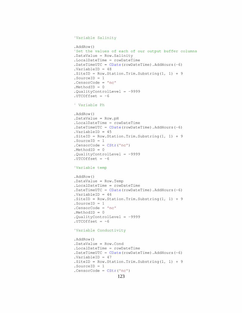
123
'Variable Salinity .AddRow() 'Set the values of each of our output buffer columns .DataValue = Row.Salinity .LocalDateTime = rowDateTime .DateTimeUTC = CDate(rowDateTime).AddHours(-6) .VariableID = 48 .SiteID = Row.Station.Trim.Substring(1, 1) + 9 .SourceID = 1 .CensorCode = "nc" .MethodID = 0 .QualityControlLevel = -9999 .UTCOffset = -6 ' Variable Ph .AddRow() .DataValue = Row.pH .LocalDateTime = rowDateTime .DateTimeUTC = CDate(rowDateTime).AddHours(-6) .VariableID = 45 .SiteID = Row.Station.Trim.Substring(1, 1) + 9 .SourceID = 1 .CensorCode = CStr("nc") .MethodID = 0 .QualityControlLevel = -9999 .UTCOffset = -6 'Variable temp .AddRow() .DataValue = Row.Temp .LocalDateTime = rowDateTime .DateTimeUTC = CDate(rowDateTime).AddHours(-6) .VariableID = 46 .SiteID = Row.Station.Trim.Substring(1, 1) + 9 .SourceID = 1 .CensorCode = "nc" .MethodID = 0 .QualityControlLevel = -9999 .UTCOffset = -6 'Variable Conductivity .AddRow() .DataValue = Row.Cond .LocalDateTime = rowDateTime .DateTimeUTC = CDate(rowDateTime).AddHours(-6) .VariableID = 47 .SiteID = Row.Station.Trim.Substring(1, 1) + 9 .SourceID = 1 .CensorCode = CStr("nc")

124
.MethodID = 0 .QualityControlLevel = -9999 .UTCOffset = -6 'Variable Disolved Oxygen .AddRow() .DataValue = Row.do .LocalDateTime = rowDateTime .DateTimeUTC = CDate(rowDateTime).AddHours(-6) .VariableID = 49 .SiteID = Row.Station.Trim.Substring(1, 1) + 9 .SourceID = 1 .CensorCode = CStr("nc") .MethodID = 0 .QualityControlLevel = -9999 .UTCOffset = -6 End With End Sub Public Overrides Sub CreateNewOutputRows() ' ' Add rows by calling AddRow method on member variable called "<Output Name>Buffer" ' E.g., MyOutputBuffer.AddRow() if your output was named "My Output" ' End Sub End Class This script is written for the following outputs:
QualityControlLevel: 4-byte signed integer DT_I4 MethodID: 4-byte signed integer DT_I4 SiteID: 4-byte signed integer DT_I4 UTCOffset: Double Precision Float DT_R8 LocalDatetime: Database timestamp [DT_DBTIMESTAMP] DateTimeUTC: Database timestamp [DT_DBTIMESTAMP] DataValue: Double Precision Float DT_R8 SourceID: 4-byte signed integer DT_I4 VariableID: 4-byte signed integer DT_I4 CensorCode: Unicode String DT_WSTR
125
APPENDIX D: SSIS DATA LOADING TUTORIAL
The Hydrologic Information System is only as strong as the services that it can provide.
For this reason we are continually looking for willing participants with data to contribute
to help quench the thirst for knowledge in the hydrologic community. This tutorial
guides you through the steps of installing an ODM database onto SQL Server and
populating the database through the use of the ODM Data Loader. This tutorial is based
off multiple HIS documents created by CUAHSI that can be found on the his.cuahsi.org
website.
Before jumping into any data loading action, we need to make sure that your
machine is configured to run all necessary components of the process. Though there are
multiple techniques that can be used to load data, this tutorial is written to instruct
loading using the following software:
Windows XP Operating System .Net Framework Microsoft SQL Server Microsoft Excel ODM Data Loader 1.1
Most of this software can be downloaded without charge from the internet or comes standard with most PC’s. Most computers only require the addition of the ODM Data Loader 1.1 and Microsoft SQL Server, in which case SQL Server Lite can be downloaded as a free alternative from Microsoft’s website and the ODM Data Loader can be downloaded from the his.cuahsi site.

126
INSTALLING AN ODM DATABASE ONTO SQL SERVER: Outline of Procedure: 1. Download the ODM 2. Attach the ODM to SQL Server 3. Examine the ODM Before actually loading, we need a place where data can be stored. The HIS uses a
database call the Observations Data Model (ODM) to house datasets. The ODM is a
relational database that uses identifiers to link metadata to data values. If you want to find
out more about the ODM documentation for Version 1.1 can be found at the follow URL:
http://his.cuahsi.org/documents/ODM1.1DesignSpecifications.pdf
So let’s get started….
The first step in attaching an ODM to SQL Server is retrieving a blank ODM database
and log file from the his.cuahsi at the following address:
http://his.cuahsi.org/software/ODM1.1BlankSQLServerSchema.zip
1. Create a folder “HISTutorial” to download and unzip the folder’s contents into. It
should contain an OD.mdf and OD_log.ldf file. It should look similar to the
screen shot below:
The “HISTutorial” folder should be at a location that can be accessed by SQL
Server. Our server has a “SQLData” directory in which we store folders
containing ODM files.
2. Next we want to attach the ODM to SQL Server.
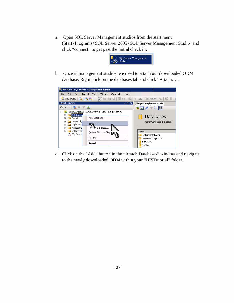
a. O(Scli
b. Oda
c. Clto
Open SQL SeStart>Programick “connect
Once in manaatabase. Righ
lick on the “the newly d
erver Managms>SQL Set” to get past
agement studht click on th
Add” buttondownloaded
127
gement studirver 2005>St the initial c
dios, we neehe databases
n in the “AttaODM within
os from the SQL Server Mcheck in.
ed to attach os tab and clic
ach Databasn your “HIS
start menu Managemen
our downloadck “Attach…
es” windowTutorial” fo
nt Studio) and
ded ODM …”.
w and navigat
lder.
d
te

3
d. Cl“Ana
ThaYou migh
. Expand thappears.
lick “ok” to Attach As” came mine “H
at’s it! Your ht want to exhe Databases
get back to tclick to renamHISTutorial,
ODM is attaxplore the ODs tab and scr
128
the “Attach Dme your dataand click “O
ached and reDM and cheroll down to
Databases” wabase to whaOk”.
eady to hold eck to ensurefind your O
window andatever you ch
your data!! e it was loadDM in the li
d under hoose, here I
ed correctlyist that
I
.

Now good
a. To“Hanemtabfie
that you havuse and fille
o look at theHISTutorial”nd click “Opmpty except bles contain elds within t
ve attached aed with data
different tab” database, een Table” tothe ControllCUAHSI prhe ODM suc
and examinea. Exit out of
129
bles within texpand the “To have the tabled Vocabulareset vocabuch as Variab
ed your ODMf SQL Server
the ODM exTables” tab able come upary tables, mulary that is uble Name and
M Database, r and move o
xpand the taband right cli
p. All tables amarked with used to fill ind Units.
it is ready to
on to the nex
b next your ck on a tableare currentlya CV. Thesen different
o be put to xt section!
e y e
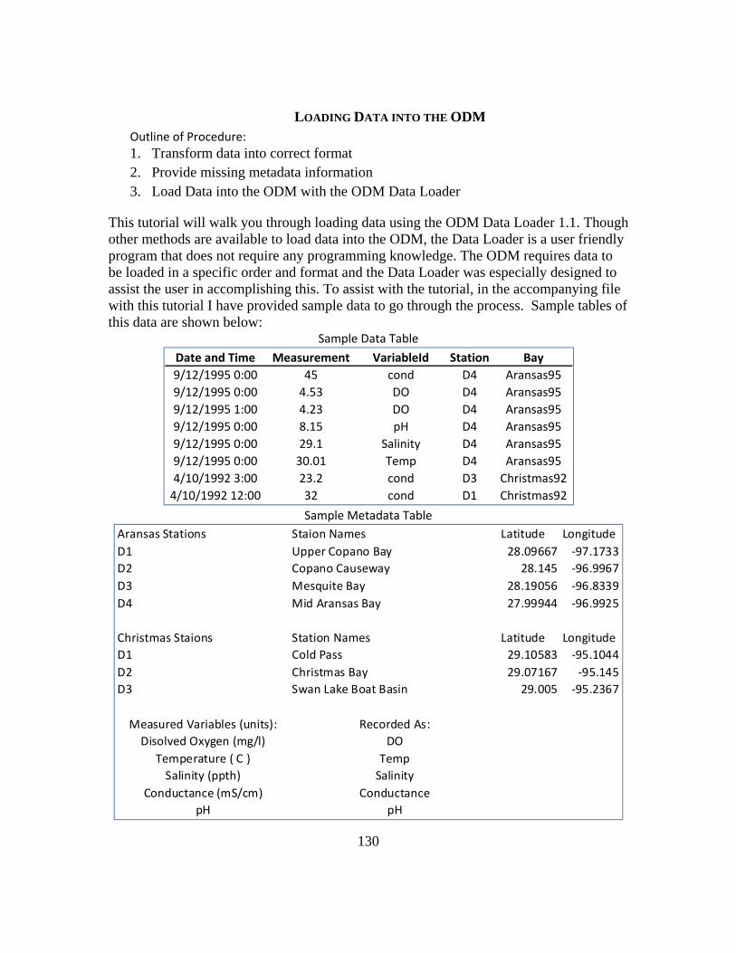
130
LOADING DATA INTO THE ODM Outline of Procedure: 1. Transform data into correct format 2. Provide missing metadata information 3. Load Data into the ODM with the ODM Data Loader
This tutorial will walk you through loading data using the ODM Data Loader 1.1. Though other methods are available to load data into the ODM, the Data Loader is a user friendly program that does not require any programming knowledge. The ODM requires data to be loaded in a specific order and format and the Data Loader was especially designed to assist the user in accomplishing this. To assist with the tutorial, in the accompanying file with this tutorial I have provided sample data to go through the process. Sample tables of this data are shown below:
Sample Data Table
Sample Metadata Table
Date and Time Measurement VariableId Station Bay9/12/1995 0:00 45 cond D4 Aransas959/12/1995 0:00 4.53 DO D4 Aransas959/12/1995 1:00 4.23 DO D4 Aransas959/12/1995 0:00 8.15 pH D4 Aransas959/12/1995 0:00 29.1 Salinity D4 Aransas959/12/1995 0:00 30.01 Temp D4 Aransas954/10/1992 3:00 23.2 cond D3 Christmas924/10/1992 12:00 32 cond D1 Christmas92
Aransas Stations Staion Names Latitude LongitudeD1 Upper Copano Bay 28.09667 ‐97.1733D2 Copano Causeway 28.145 ‐96.9967D3 Mesquite Bay 28.19056 ‐96.8339D4 Mid Aransas Bay 27.99944 ‐96.9925
Christmas Staions Station Names Latitude LongitudeD1 Cold Pass 29.10583 ‐95.1044D2 Christmas Bay 29.07167 ‐95.145D3 Swan Lake Boat Basin 29.005 ‐95.2367
Measured Variables (units): Recorded As:Disolved Oxygen (mg/l) DO
Temperature ( C ) TempSalinity (ppth) Salinity
Conductance (mS/cm) ConductancepH pH
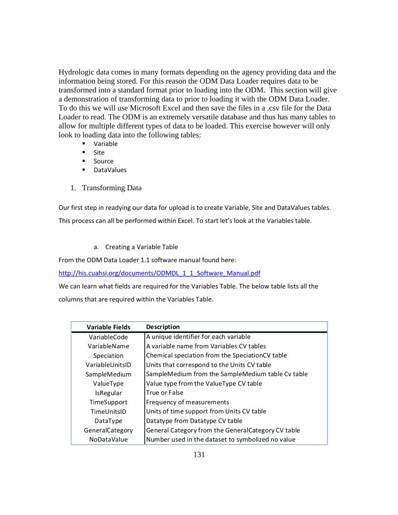
131
Hydrologic data comes in many formats depending on the agency providing data and the information being stored. For this reason the ODM Data Loader requires data to be transformed into a standard format prior to loading into the ODM. This section will give a demonstration of transforming data to prior to loading it with the ODM Data Loader. To do this we will use Microsoft Excel and then save the files in a .csv file for the Data Loader to read. The ODM is an extremely versatile database and thus has many tables to allow for multiple different types of data to be loaded. This exercise however will only look to loading data into the following tables:
Variable Site Source DataValues
1. Transforming Data
Our first step in readying our data for upload is to create Variable, Site and DataValues tables.
This process can all be performed within Excel. To start let’s look at the Variables table.
a. Creating a Variable Table
From the ODM Data Loader 1.1 software manual found here:
http://his.cuahsi.org/documents/ODMDL_1_1_Software_Manual.pdf
We can learn what fields are required for the Variables Table. The below table lists all the
columns that are required within the Variables Table.
Variable Fields Description
VariableCode A unique identifier for each variableVariableName A variable name from Variables CV tablesSpeciation Chemical speciation from the SpeciationCV table
VariableUnitsID Units that correspond to the Units CV tableSampleMedium SampleMedium from the SampleMedium table Cv table
ValueType Value type from the ValueType CV tableIsRegular True or False
TimeSupport Frequency of measurementsTimeUnitsID Units of time support from Units CV tableDataType Datatype from Datatype CV table
GeneralCategory General Category from the GeneralCategory CV tableNoDataValue Number used in the dataset to symbolized no value

132
From the data provided in our metadata table, controlled vocabulary tables and knowledge
about this data, the following table can be created.
We still need to populate the VariableCode field to complete this table. In many agencies
standard codes are created for variables throughout all studies. These codes, as long as any
unique designation can be used as a variable code. Since the ODM Data Loader can use
VariableCodes to link a data value to a variable in the variable table let’s use the VariableIDs
already used in this dataset. Implementing these identifiers within the table our completed
Variable Table is completed and ready to be uploaded with the Data Loader.
VariableCode VariableName Speciation VariableUnitsId SampleMediumSpecific conductance, filtered Not Applicable 269 Surface Water
Oxygen, Dissolved Not Applicable 199 Surface WaterpH, filtered Not Applicable 137 Surface WaterSalinity Not Applicable 306 Surface Water
Temperature Not Applicable 96 Surface Water
ValueType IsRegular TimeSupport TimeUnitsID DataType GeneralCategory NoDataValueField Observation TRUE 1 103 Continuous Water Quality ‐9.99Field Observation TRUE 1 103 Continuous Water Quality ‐9.99Field Observation TRUE 1 103 Continuous Water Quality ‐9.99Field Observation TRUE 1 103 Continuous Water Quality ‐9.99Field Observation TRUE 1 103 Continuous Water Quality ‐9.99
VariableCode VariableName Speciation VariableUnitsId SampleMediumCond Specific conductance, filtered Not Applicable 269 Surface WaterDO Oxygen, Dissolved Not Applicable 199 Surface WaterpH pH, filtered Not Applicable 137 Surface Water
Salinity Salinity Not Applicable 306 Surface WaterTemp Temperature Not Applicable 96 Surface Water
ValueType IsRegular TimeSupport TimeUnitsID DataType GeneralCategory NoDataValueField Observation TRUE 1 103 Continuous Water Quality ‐9.99Field Observation TRUE 1 103 Continuous Water Quality ‐9.99Field Observation TRUE 1 103 Continuous Water Quality ‐9.99Field Observation TRUE 1 103 Continuous Water Quality ‐9.99Field Observation TRUE 1 103 Continuous Water Quality ‐9.99
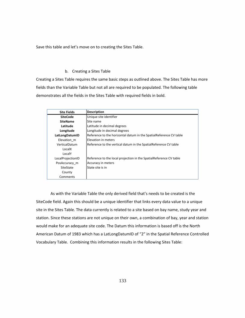
133
Save this table and let’s move on to creating the Sites Table.
b. Creating a Sites Table
Creating a Sites Table requires the same basic steps as outlined above. The Sites Table has more
fields than the Variable Table but not all are required to be populated. The following table
demonstrates all the fields in the Sites Table with required fields in bold.
As with the Variable Table the only derived field that’s needs to be created is the
SiteCode field. Again this should be a unique identifier that links every data value to a unique
site in the Sites Table. The data currently is related to a site based on bay name, study year and
station. Since these stations are not unique on their own, a combination of bay, year and station
would make for an adequate site code. The Datum this information is based off is the North
American Datum of 1983 which has a LatLongDatumID of “2” in the Spatial Reference Controlled
Vocabulary Table. Combining this information results in the following Sites Table:
Site Fields DescriptionSiteCode Unique site identifierSiteName Site nameLatitude Latitude in decimal degreesLongitude Longitude in decimal degrees
LatLongDatumID Reference to the horizontal datum in the SpatialReference CV tableElevation_m Elevation in metersVerticalDatum Reference to the vertical datum in the SpatialReference CV table
LocalXLocalY
LocalProjectionID Reference to the local projection in the SpatialReference CV tablePosAccuracy_m Accuracy in meters
SiteState State site is inCounty
Comments

134
1. Creating DataValues Tables
Again to create a DataValues table we need to refer to the require fields layed out in the ODM
Data Loader specifications. The DataValues table, being the central table within the ODM has a
primary job of housing data values and linking them to other metadata tables. For this reason
many of the fields within the DataValues Table act as connectors to other tables. Again the
required fields are in bold, but it is recommended as many fields be filled out so as best describe
the data.
For our data the only fields we need to add to the existing DataValues table is CensorCode,
MethodID, SourceID and QualityControlLevel ID.
SiteCode SiteName Latitude Longitude LatLongDatumID SiteStateAransas95_D1 Upper Copano Bay 28.09666667 ‐97.17333333 2 TexasAransas95_D2 Copano Causeway 28.145 ‐96.99666667 2 TexasAransas95_D3 Mesquite Bay 28.19055556 ‐96.83388889 2 TexasAransas95_D4 Mid Aransas Bay 27.99944444 ‐96.9925 2 TexasChristmas92_D1 Cold Pass 29.10583333 ‐95.10444444 2 TexasChristmas92_D2 Christmas Bay 29.07166667 ‐95.145 2 TexasChristmas92_D3 Swan Lake Boat Basin 29.005 ‐95.23666667 2 Texas
DataValue DescriptionValueAccuracyLocalDateTimeUTCOffset Universal Time Clock OffsetDateTimeUTC Universal Time Clock timeSiteCode SiteCode used in Sites TableVariableCode VariableCode used in Variables TableOffsetValueOffsetTypeID Link to OffsetType TableCensorCode From CensorCV TableQualifierID Link to qualifier tableMethodID Link to Method TableSourceID Link to Source TableSampleID Link to Sample TableQualityControlLevelID Link to Quality Control Level TableGroupID Link to GroupID Table

Since
which
ODM
one. A
comp
inform
Reope
down
In the
autom
Don’t
since
anoth
our M
none of our v
h stands for n
and can be o
A Source ID a
pared to the o
mation into th
en SQL Serve
n to the Sourc
e table that op
matically fill in
t be alarmed i
you have yet
her table of ci
MetadataID m
values are ce
ot censored.
opened as any
nd MethodID
others we hav
he ODM.
r and navigat
ce tab, right c
pens, click un
n) and enter t
if you see red
t to fill in all th
tation inform
meaning that t
nsored, we w
Again, all con
y other table
D also need to
ve already cre
te to and expa
lick and choo
nder the “Org
the source inf
d warning circ
he required s
mation. Since
the MetaData
135
will use the ce
ntrolled voca
in the ODM u
o be created.
eated we may
and your ODM
ose “open tab
anization” fie
formation pro
cles, these are
source inform
we will not b
a is unknown.
ensor controll
bulary tables
using the proc
Since these t
y just want to
M. Expand th
ble”.
eld title (skip
ovided below
e simply tellin
mation. The M
e filling out th
.
led vocabular
are housed w
cedure outlin
tables are rela
o manually inp
e Tables tab a
the SourceID
w or your own
ng you to con
MetadataID re
his table we c
ry term “nc”
within the
ned in section
atively small
put this
and navigate
field, this wi
n variation.
tinue writing
fers to
can put a 0 fo
n
ll
g
or

136
Like the Metadata table we do not have information on the methods used to collect this data so
our MethodID will also be 0. While we have the ODM open, let’s open the QualityControlLevel
Table to view what we best think describes our data. The table looks similar to the one below.
As you can see we have several quality levels to chose from.
For this data the most suitable would be level 1, “Raw Data” since there has been no quality
control performed on the data, thus the QualityControlLevelID would be 1.
The final field we need to fill in is either the UTCoffset or DateTimeUTC. We only need to
complete one of these fields and the ODM Data Loader will automatically populate the other.
Since this data comes from the Central Time Zone, its UTCoffset for every point is ‐6. This data
has been corrected for differences in daylight savings time but be aware in the future for data
that has not.
Finally putting all these fields together we should create a DataValues Table that looks
something like the following:

Great
to go
We w
findin
HIS>O
A “Ne
ODM
passw
Local9/12/9/12/9/12/9/12/9/12/9/12/9/12/9/12/9/12/9/12/9/12/9/12/9/12/
t work! After
ahead and lo
2.
will be using th
ng it and open
ODM DL 1.1.
ew Database C
being served
word and click
DateTime DataV/1995 0:00 4.5/1995 0:00 8.1/1995 0:00 29./1995 0:00 30.0/1995 0:00 45/1995 1:00 ‐9.9/1995 1:00 8.1/1995 1:00 29./1995 1:00 30.0/1995 1:00 45/1995 2:00 4.2/1995 2:00 8.1/1995 2:00 29
making sure
oad this data!
Loading Da
he ODM Data
ning up the so
Connection”
d on SQL Serv
k “Save Chang
Value VariableCode3 DO5 pH1 Salinity01 Temp5 cond99 DO3 pH2 Salinity01 Temp5 cond2 DO2 pH9 Salinity
each of these
ta
a Loader versi
oftware. To a
box appears
er. Fill in the
ges”.
e SiteCodeAransas95_D4Aransas95_D4Aransas95_D4Aransas95_D4Aransas95_D4Aransas95_D4Aransas95_D4Aransas95_D4Aransas95_D4Aransas95_D4Aransas95_D4Aransas95_D4Aransas95_D4
137
e tables is sav
ion 1.1 to loa
ccess the pro
that allows th
address of yo
UTCOffset Cen‐6‐6‐6‐6‐6‐6‐6‐6‐6‐6‐6‐6‐6
ved in its own
d these three
ogram go to S
he ODM Data
ou server, OD
sorCode SourceIDnc 1nc 1nc 1nc 1nc 1nc 1nc 1nc 1nc 1nc 1nc 1nc 1nc 1
n .csv file, we
e tables so ou
tart>All Progr
a Loader to co
DM Name and
D MethodID Qua0000000000000
will be ready
ur first task is
rams>CUAHS
onnect to you
d user ID and
lityConrolLevelID1111111111111
y
SI
ur
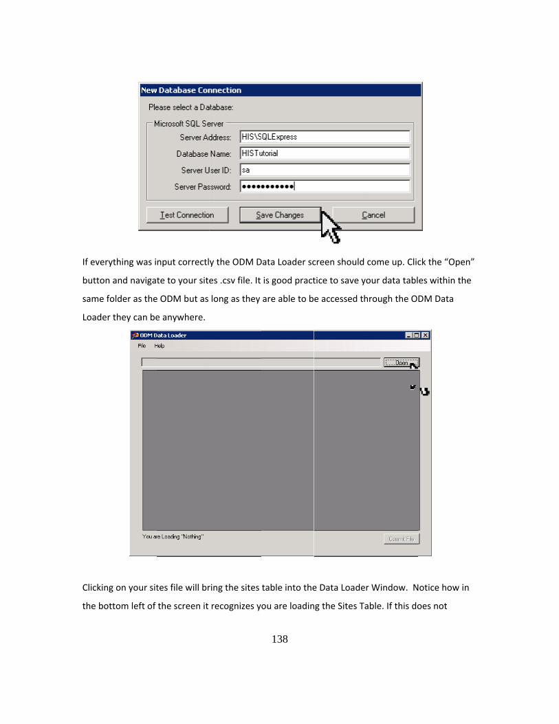
If eve
butto
same
Loade
Clickin
the bo
rything was i
n and navigat
folder as the
er they can be
ng on your sit
ottom left of
nput correctl
te to your sit
e ODM but as
e anywhere.
tes file will br
the screen it
y the ODM D
es .csv file. It
long as they
ring the sites
recognizes y
138
Data Loader sc
is good pract
are able to b
table into the
ou are loadin
creen should
tice to save y
e accessed th
e Data Loade
ng the Sites Ta
come up. Clic
our data tabl
hrough the O
r Window. N
able. If this do
ck the “Open
es within the
DM Data
otice how in
oes not
”
e
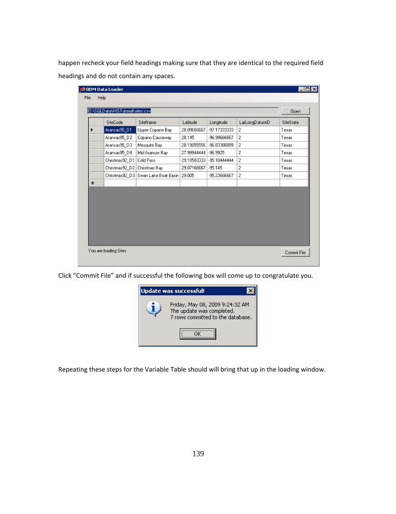
139
happen recheck your field headings making sure that they are identical to the required field
headings and do not contain any spaces.
Click “Commit File” and if successful the following box will come up to congratulate you.
Repeating these steps for the Variable Table should will bring that up in the loading window.

140
Again click “Commit File” to load this into your ODM. Finally, open your DataValues Table and
commit this file to your database.

141
After a couple of second all 26,544 data values are loaded into your ODM
Congratulations you have loaded data into an ODM Database! Feel free to examine the ODM
tables now populated with your data in the methods described above.

142
GLOSSARY:
Data Manager: A person responsible for the upload and upkeep of data on an HIS Server
Data Service: An online database accessible through web services
Data Value: A recorded value
HIS: A generic term used to describe a system for accessing and synthesizing hydrologic
information
HIS Central: A catalog of HIS Registry metadata
HIS Desktop: A desktop application that can be utilized for hydrologic data access and
discovery
HIS Registry: A registry of HIS data services
HIS Server: A server used to host and publish HIS data services
Metadata: Descriptive data about a data service such as variable name and method
Observation Data Model: A relational database built to store hydrologic temporal data
Relational Database: A database structure that relies on linked tables
WaterOneFlow: A set of four functions used to read the ODM whose output is in
WaterML
Web Services: Software that allows machine to machine interaction through the web
143
BIBLIOGRAPHY
Alameda, J. C. (2006). Web Services. In P. Kumar, J. C. Alameda, P. Bajcsy, M. Folk, & M. Markus, Hydroinformatics (p. 171). Boca Rotan, Fl: Taylor and Francis Group. Beran, B. (2007). HydroSeek: An Ontology-Aided Data Discovery System for Hydrologic. Retrieved from http://idea.library.drexel.edu/bitstream/1860/1873/1/Beran_Bora.pdf Center for Spatial Information Science and System. (n.d.). GeoBrain Online Analysis System (GeOnAS) User Guide. Retrieved from http://geobrain.laits.gmu.edu:8099/OnAS/User_Guide.pdf Dicks, S. (Nov. 2008). An Integrated Approach to Water Managing Water Resources Data at the Southwest Florida Water Management District. Water Resources Impact , 10-13. Han et al. (2008). Design and Implementation of GeoBrain Online Analysis. Retrieved from http://www.springerlink.com/content/c303j5070l742358/fulltext.pdf Horsburgh, J. &. (2008). ODM Data Loader Version 1.1. Retrieved from http://his.cuahsi.org/documents/ODMDL_1_1_Software_Manual.pdf Jantzen, T. L. (2007). Implementation of a State Hydrologic Information System. Austin, Tx: Center for Research of Water Resources at the University of Texas Austin. Kumar et al. (2006). Hydroinformatics. Boca Raton, FL: Taylor & Francis. Maidment, D. (2008). CUAHSI Hydrologic Information System: Overview of Version 1.1. Retrieved from http://his.cuahsi.org/documents/HISOverview.pdf Maidment, D. (2008). CUAHSI Hydrologic Information System: Overview of Version 1.1. Austin, Tx: University of Texas at Austin. Maidment, D. (2005). Hydrologic Information System Version 1. National Research Council. (1991). Oppertunities in the Hydrologic Sciences. Washington DC: National Academy Press. Tarboton et al. (2008). ODM 1.1 Design Specification. Valentine, D., Whitenack, T., Whiteaker, T., & To, E. (2008). Configuring Web Services for an Observations Database, Version 1. Whiteaker, T. (2008). HydroExcel 1.1 Software Manual. University of Texas at Austin Center for Research in Water Resources . Zaslavsky, I., Valentine, D., & Whiteaker, T. (2007). CUAHSI WaterML. Open Geospatial Consortium.

144
145
VITA
Bryan Jacob Enslein was born on October 23, 1984 in North Haven, Connecticut
to Mark and Marianne Enslein, and is the younger brother of Kristin Enslein. He
graduated from North Haven High School in 2003 and attended Villanova University
where he achieved a degree in Civil and Environmental Engineering in 2007. There he
became interested in Water Resources while taking part in several international service
projects. Between studies, Bryan worked for the Northwest Youth Corps where he led a
troupe of teenage boys working on environmental restoration projects along the Oregon
Coast. Upon graduating the University of Texas, Bryan plans on working overseas with
the Peace Corps.
Permanent Address: 75 Round Hill Road
North Haven, CT 06473
This thesis was typed by the author.