the implementation and testing of the santoss … implementation and testing of the santoss sand...
TRANSCRIPT

The implementation and testing of the SANTOSS sand transport model in Delft3D Author Roelof Veen


The implementation and testing of the SANTOSS sand transport model in Delft3D
1204017-000 © Deltares, 2014, B
Roelof Veen


The implementation and testing of the SANTOSS sand transport model in
Delft3D
Supervised by
Department of Water Engineering and Management Faculty of Engineering Technology
University of Twente
Friday, 14 Februari 2014
Author R. Veen Exam Committee Graduation supervisor dr. ir. J. S. Ribberink University of Twente Daily supervisor UT J. van der Zanden MSc. University of Twente Daily supervisor Deltares dr. ir. J. J. van der Werf Deltares


Title The implementation and testing of the SANTOSS sand transport model in Delft3D Client UNIVERSITY OF TWENTE
Project 1204017-000
Reference 1204017-000-ZKS-0001
Pages 82
The implementation and testing of the SANTOSS sand transport model in Delft3D
Keywords Nearshore processes, sediment transport, SANTOSS model, Delft3D, LIP experiment. Summary This study aims to assess and improve the way Delft3D models wave-driven cross-shore sand transport. This is done by implementing and testing the SANTOSS near bed transport model using reliable data from full-scale wave flume experiments. The Delft3D assessment was done by modelling an erosive and accretive case of the LIP experiment. This shows that the modelling results with the SANTOSS model are promising for the accretive case and the erosive case offshore of the breaker bar, and better then when using the current state-of-the-art Van Rijn (2007ab) transport model. The transport rates in the erosive case onshore of the breaker bar were not well predicted with the SANTOSS model and the Van Rijn (2007ab) model does better here. The SANTOSS model in Delft3D can be improved by making the combination of the SANTOSS near bed transport model and the current related suspended transport model of Van Rijn (2007b) more consistent by determining the suspended transport above the wave boundary layer. An improvement for the SANTOSS model would be to implement the effects of turbulence due to breaking waves. References Version Date Author Initials Review Initials Approval Initials feb. 2014 R. Veen J.J. van der Werf F.M.J. Hoozemans State final


14 February 2014, final
The implementation and testing of the SANTOSS sand transport model in Delft3D
Preface
This thesis is the final step in finishing my Master Water Engineering and Management at the University of Twente and was carried out at Deltares. The topic of the thesis relates to the prediction of sand transport in the coastal zone with a coastal morphological model. While working on the thesis I learned a lot about programming in, working with and analyzing the results in a morphological model and the reading and writing of a scientific report. I liked working on all these aspects although each topic came with new challenges and some frustrations. I would like to thank everybody how supported me during this period in one way or another. First of all, my supervisors, Jan Ribberink, Jebbe van der Werf and Joep van der Zanden, for their interest in my research and the useful and interesting comments on my work. Especially my supervisor at Deltares, Jebbe, for always having the time to answer any question or for discussing the latest results. As well as my supervisor at the university, Joep, for the interesting meetings we had over this period. Another person is Adri Mourits who supported me in the work of programming in Delft3D and helping me with debugging or to think about best ways to get the SANTOSS model in Delft3D. Also special thanks to my brother and father, Alex en Bart, how helped me in the last weeks in the refinement of the text of this thesis. I’m very grateful for the chance to carry out my thesis at Deltares. This gave me the opportunity to meet new and interesting people and work in a company in which a lot of knowledge about hydrodynamic and sand transport in the coastal zone is available. Also the attitude of sharing knowledge through the lunch lectures, which were sometimes a bit outside my scopes, was very interesting en educational. I want to thank my fellow students at Deltares for their good company during the coffee brakes, lunches and the occasional drinks after work and my friends in Enschede for the great 7 years. Last but not least, I like to thank my parents, brothers, sister and my girlfriend Armelle, for always being there for me and helping me to get where I am today. I hope you enjoy reading this report. Roelof Veen Delft, February 2014

14 February 2014, final
The implementation and testing of the SANTOSS sand transport model in Delft3D
Summary
The coastal zone is an important social economical area for humans, which needs protection. Coastal engineers use morphological models to understand the morphological system and predict coastal erosion and sedimentation caused by both natural processes and human interaction. To improve sand transport modelling continuous research is being conducted trying to gain a better understanding of the processes how sand is transported and it is subsequently attempted to integrate this new knowledge into morphological models. The SANTOSS research project developed a new ‘semi-empirical’ model for sand transport near the sea bed in coastal marine environment. This new transport model is a semi-unsteady model based on the half-wave cycle concept with bed shear stress as the main forcing parameter and is derived for non-breaking waves and/or currents. Under these conditions it is assumed that all the sediment is transported within the wave boundary layer. The SANTOSS model does not account for suspended sediment outside the wave boundary layer (Van der A et al., 2013). The objective of this study is to assess and improve the way Delft3D models wave-driven cross-shore sand transport. This is done by implementing and testing the SANTOSS transport model using reliable data from full-scale wave flume experiments. To implement the SANTOSS model in Delft3D, the SANTOSS model needed to be written in the program language FORTRAN. Three conceptual additions were made for the SANTOSS model, these additions were needed to embedded the SANTOSS model in Delft3D. In this way the SANTOSS model could be implemented in Delft3D and could be applied to coastal conditions. The first addition was changing the SANTOSS model to determine sand transport in current dominant flow. The second addition was adding a method to determine the wave velocity and acceleration skewness from the wave height, wave length and water depth by Ruessink et al. (2012) and Abreu et al. (2010). The third was applying a longitudinal slope effect of Apsley and Stansby (2008) to the critical shear stress in the direction of the shear stress for the calculation of sand transport on slopes. The embedding of the SANTOSS model concerned three topics. Firstly, that the orientation between the SANTOSS model and Delft3D was different. Secondly, the slope effect on the transport rates and direction. Therefore the available method of Bagnold (1996) was used for the longitudinal slope effect and the method of Van Rijn (1993) was used for the lateral slope effect. Thirdly, the suspended wave model of Van Rijn (2007b) is used to calculate the suspended transport in combination with near bed transport of the SANTOSS model. The assessment of the sediment transport of Delft3D with the implemented SANTOSS sand transport model was done by modelling two cases of the LIP experiment without morphological updating. In one case wave conditions for beach erosion were used and the other case wave conditions for beach accretion were used. In the erosive case the near bed transport offshore of the breaker bar with the SANTOSS model showed reasonable agreement with the measurements. Onshore of the breaker bar measurements indicated a peak onshore. The SANTOSS model computed transports in contrast showed offshore transport. The offshore transports of the SANTOSS model seemed to be caused by combination of the decrease in the phase lag effect and an increase of offshore directed bed shear stress. The results of the SANTOSS model in the accretive case showed that offshore of the breaker bar the near bed transport gradually increased with decreasing depth what was expected. However, one measurement at 65 m showed an offshore transport. Onshore of the breaker bar the near bed transport computed with the SANTOSS seem to agree reasonable

14 February 2014, final
The implementation and testing of the SANTOSS sand transport model in Delft3D
with the measurements but seems to be somewhat underestimated. This could be due to the wave related suspended transport that takes place outside the wave boundary layer. At the end of the surf zone near the shore there is some measured and calculated transport. At the breaker bar the SANTOSS model showed a strong effect to the shift in bed regime and thereby underestimates the onshore transport. From the comparison of the SANTOSS model with the measured or computed hydrodynamic input two conclusions can be made. The first is that the prediction of the hydrodynamics has influence on the orbital velocities and thus influence on the transports. The second, that modelling better hydrodynamics does not always leads to better prediction of the sand transport with the SANTOSS model. To improve the SANTOSS model in Delft3D three proposals have been made. The first is to look at the parameterization of the velocity- and acceleration skewness. Secondly, make the combination of the SANTOSS model and the current related suspended transport model of Van Rijn (2007b) more consistent by determining the suspended transport above the wave boundary layer. The third improvement is to implement the effects of turbulence due to breaking waves. Additional research that can be done, is performing an extensive sensitivity analysis for a better understanding of the SANTOSS model or the modelling of additional cases either flume experiments (e.g. Yoon and Cox, 2010) or real beach cases (e.g. Aagaard and Jensen, 2013) where high detailed data are available.


14 February 2014, final
The implementation and testing of the SANTOSS sand transport model in Delft3D
i
Contents
1 Introduction 1 1.1 Research background 1 1.2 Research objective and questions 1 1.3 Methodology 2 1.4 Thesis outline 2
2 Research background 3 2.1 Hydrodynamics 3
2.1.1 Wave shape and orbital motion 3 2.1.2 Currents 4 2.1.3 Wave breaking 4
2.2 Sediment transport 5 2.2.1 Bedform regimes 5 2.2.2 Bed shear stress 5 2.2.3 Phase lag effect 6 2.2.4 Progressive surface wave effect 6
2.3 Delft3D 6 2.3.1 Hydrodynamics 7 2.3.2 Roller model 8 2.3.3 Sediment transport 8
2.4 The SANTOSS model 12 2.5 Conclusion 14
3 SANTOSS model in FORTRAN code 15 3.1 Conceptual expansion of the SANTOSS model 15
3.1.1 Current dominated flow 15 3.1.2 Orbital characteristics 17 3.1.3 Slope effect on critical shear stress 20
3.2 SANTOSS model in FORTRAN code 21 3.3 Embedding SANTOSS in Delft3D 24
3.3.1 Orientation 24 3.3.2 Slope effect on transport 26 3.3.3 Suspended transport 26
3.4 Conclusions 27
4 Model assessment 29 4.1 LIP experiment 29 4.2 Model set-up 31
4.2.1 Computational grid 31 4.2.2 Initial and boundary conditions 31 4.2.3 Wave and bottom settings 31
4.3 Hydrodynamic Calibration 32 4.4 Sand transport 37
4.4.1 Calculation measured transport 37 4.4.2 Erosive beach conditions 38 4.4.3 Accretive case 42 4.4.4 Phase lag, slope and acceleration skewness effect 46

14 February 2014, final
ii
The implementation and testing of the SANTOSS sand transport model in Delft3D
4.4.5 Influence hydrodynamic on SANTOSS 47 4.5 Conclusions 49
5 Discussion 51 5.1 Conceptual additions SANTOSS 51 5.2 Implementation SANTOSS in Delft3D 52 5.3 Modeling with SANTOSS in Delft3D 52
6 Conclusions 55
7 Recommendations 59
8 References 61 Appendices
A Calibration parameters roller model I
B Approximation wave form for skewed waves III
C Description FORTRAN codes VI
D Results processes within the SANTOSS model X

14 February 2014, final
The implementation and testing of the SANTOSS sand transport model in Delft3D
1
1 Introduction
The coastal zone is an important social economical area for humans, which needs protection. Coastal engineers use morphological models to understand the morphological system and predict coastal erosion and sedimentation caused by both natural processes and human interaction. These models are used in the design and for management decisions in the coastal zones. The uncertainties, associated with the predictions of these models, are, however relatively large.
1.1 Research background Morphological models are used to gain a better understanding and to predict the near shore sediment transport. Models that provide results within a factor two of the measured data are described as good models (Van der A et al., 2013; Hasan and Ribberink, 2010), hence there still is a substantial degree of uncertainty of the modelled process. Given the uncertainty in these models, it is challenging to make adequate management decisions and designs for coastal zones. The morphological model Delft3D consists of coupled models for waves, currents, sediment transport and bed level changes. The sediment transport model usually consists of two parts, the suspended sediment transport and the (near) bed sediment transport model. To improve sand transport modelling continuous research is being conducted trying to gain a better understanding of the processes how sand is transported and it is subsequently attempted to integrate this new knowledge into morphological models. The SANTOSS research project started with the goal of establishing a new ‘semi-empirical’ model for sand transport near the sea bed in coastal marine environment. This new transport model is a semi-unsteady model based on the half-wave cycle concept with bed shear stress as the main forcing parameter and is derived for non-breaking waves and/or currents. Under these conditions it is assumed that all the sediment transport is transported within the wave boundary layer. The SANTOSS model does not account for suspended sediment outside the wave boundary layer (Van der A et al., 2013).
1.2 Research objective and questions The objective of this research is to combine the developed SANTOSS model in the morphodynamic model Delft3D. For this the following research objective has been formulated. “The objective of this study is to assess and improve the way Delft3D models wave-driven cross-shore sand transport by implementing and testing the SANTOSS transport model using reliable data from full-scale wave flume.” For achieving the research objective as stated above four research questions are formulated. 1 How to extent the SANTOSS model conceptually? 2 How should the SANTOSS model be implemented in Delft3D? 3 How does the SANTOSS model within Delft3D perform compared to the measurements
of net sand transport of controlled wave flume experiments? 4 How does the SANTOSS model within Delft3D perform compared to the default Van
Rijn model (2007ab)?

14 February 2014, final
The implementation and testing of the SANTOSS sand transport model in Delft3D
2
1.3 Methodology To answer the first two research questions the SANTOSS model and Delft3D are studied through literature (e.g. Van der A et al., 2013, Deltares, 2012). By studying these models estimation can be made witch processes are not included in the SANTOSS model, however are needed when used in Delft3D. To extent the SANTOSS model with these processes a method should be found in literature that can be used within the SANTOSS model. The second research question is answered by implementing the SANTOSS model in Delft3D in five steps. The first step is to convert the available MATLAB code of the SANTOSS model to FORTRAN code (the program language of Delft3D). Secondly the stand alone FORTRAN code is tested with dummy data and compared to the results of the MATLAB code by running the same dummy data, to confirm that the conversion is successful. Thirdly, the additional extensions from the first research question are added to the SANTOSS model. Next the input and output of the FORTRAN code is coupled to the parameters in Delft3D. Finally Delf3D with the SANTOSS model will be executed in order to check if the coupling of the in- and outputs has been successful. The third and fourth research question is an assessment of the Delft3D model with the SANTOSS model of a controlled wave flume experiments. To analyse the model for different conditions two experiments are selected, namely the LIP-1B and the LIP-1C case. The wave in the LIP-1B case causes the beach to erode where the waves in the LIP-1C case causes an accretive beach. The LIP-experiment dataset contains: wave characteristics, water set up, velocity profiles, concentration profiles and bed level evolution. The two cases are modelled into Delft3D and calibrated with the wave characteristic data and the water level setup. The influence of the hydrodynamics on the assessment of the transport model is minimized by the calibration of the hydrodynamic model. To answer the third research question the results of the LIP experiments from Delft3D with the SANTOSS model are compared to the measured net sand transport results. The processes within the SANTOSS model are explored, to analyse how the transports within the SANTOSS model are calculated. Also the results of the SANTOSS model in Delft3D are compared to the SANTOSS model with the measured hydrodynamics as input. This is to investigate the influence of the calculated hydrodynamic on the SANTOSS model.
The fourth research question concerns the comparison of the LIP experiments modelled in Delft3D with the SANTOSS or Van Rijn sand transport model. By comparing these two sand transport models in Delft3D an indication can be made if the implementing the SANTOSS model is an improvement for the sand transport modelling in Delft3D.
1.4 Thesis outline In the following chapters the research background of the thesis is present. Chapter two describes the relevant research background. Chapter three describes the conceptual extensions of the SANTOSS model, the conversion of the SANTOSS model to FORTRAN code and the implementation of the SANTOSS model in Delft3D. In the fourth chapter the simulation of two cases of the LIP experiment with Delft3D are described and the comparison of the SANTOSS model with the measurements and the Van Rijn model. The fifth chapter contains the discussion followed by conclusions in chapter six. The last chapter includes the recommendations.
14 February 2014, final
The implementation and testing of the SANTOSS sand transport model in Delft3D
3
2 Research background
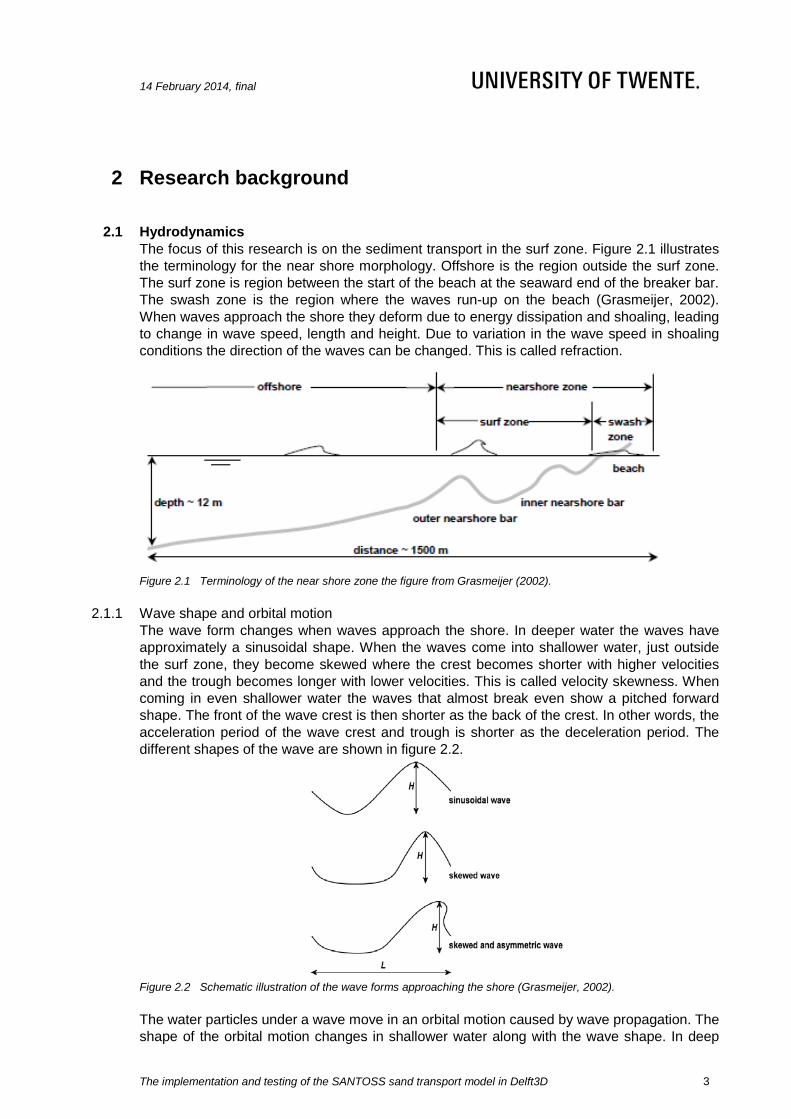
2.1 Hydrodynamics The focus of this research is on the sediment transport in the surf zone. Figure 2.1 illustrates the terminology for the near shore morphology. Offshore is the region outside the surf zone. The surf zone is region between the start of the beach at the seaward end of the breaker bar. The swash zone is the region where the waves run-up on the beach (Grasmeijer, 2002). When waves approach the shore they deform due to energy dissipation and shoaling, leading to change in wave speed, length and height. Due to variation in the wave speed in shoaling conditions the direction of the waves can be changed. This is called refraction.
Figure 2.1 Terminology of the near shore zone the figure from Grasmeijer (2002).
2.1.1 Wave shape and orbital motion The wave form changes when waves approach the shore. In deeper water the waves have approximately a sinusoidal shape. When the waves come into shallower water, just outside the surf zone, they become skewed where the crest becomes shorter with higher velocities and the trough becomes longer with lower velocities. This is called velocity skewness. When coming in even shallower water the waves that almost break even show a pitched forward shape. The front of the wave crest is then shorter as the back of the crest. In other words, the acceleration period of the wave crest and trough is shorter as the deceleration period. The different shapes of the wave are shown in figure 2.2.
Figure 2.2 Schematic illustration of the wave forms approaching the shore (Grasmeijer, 2002). The water particles under a wave move in an orbital motion caused by wave propagation. The shape of the orbital motion changes in shallower water along with the wave shape. In deep

14 February 2014, final
The implementation and testing of the SANTOSS sand transport model in Delft3D
4
water the water particles move in a circular shape, where they changes form circular to elliptic in shallower water. The motion decreases in depth where in shallow the shape of the elliptic motion changes into a horizontal motion.
Figure 2.3 Change of orbital motion under waves approaching the shore (Grasmeijer, 2002). The changing shape of the path of the water practices is related to the changing wave form. Under the velocity skewed waves the shoreward velocity of the water particles has a shorter duration with higher velocities where the off shore velocity of the water particles has a longer duration and a lower velocity. The onshore motion can be related to the wave crest and the offshore motion to the wave trough. Under the pitched forward (acceleration skewed) waves the acceleration in the movement of the partial is asymmetric. This implies that the acceleration period of the onshore motion has a shorter duration as the deceleration period. For the offshore motion this implies that the deceleration period has a shorter duration as the acceleration period. To compute the wave shapes and orbital motion of the water partials a parameter for the velocity skewness and one for the acceleration skewness are needed.
2.1.2 Currents Near shore currents are commonly described by cross-shore and longshore currents. The cross-shore current is an onshore mass flux near the surface of the water column caused by the difference between the mass fluxes of the wave crest and trough. The coast is a closed boundary so the net transport at the coast needs to be zero. There for the onshore flux at the surface of the water column is compensated by the undertow, an offshore directed mean current near the bed. This typically occurs during the high energy wave conditions (Svenden, 1984). This effect is relative small for non-breaking waves whereas for breaking waves the onshore transport and thus the undertow are relative large. The longshore current can be induced by waves that arrive at an angle to the shoreline or due to the tidal induced longshore gradient in the mean water level. The waves that arrive in an angle to the coast can be described by a longshore and cross-shore component where the longshore component generates a mass flux (due to the difference between wave crest and trough) in the direction of the component. Because there is no boundary as in the cross-shore direction the current caused by the mass flux is the same direction over the whole water column. The rise and fall of the water level due to the ebb and flood, what causes a gradient in the surface level and thus leads to the tidal longshore current in the water. At the same, time as the tide changes between ebb and flood, the tidal current changes from direction.
2.1.3 Wave breaking Wind driven ocean waves that approach the shore can break. The energy of these waves is dissipated as heat, sound and mixing of water and sediment (Wright et al., 1999). In shallow water, the waves will break if the relative height exceeds a certain critical value. The relative

14 February 2014, final
The implementation and testing of the SANTOSS sand transport model in Delft3D
5
height is the wave height relative to the water depth, where the waves breaks for 𝐻𝑑
> 𝛾 with γ=[0.7-1.3] the waves breaks with γ=[0.7-1.3] (Van Rijn, 2011). There are different types of breaking waves depending on the steepness of the wave and the steepness of the beach. Battjes (1974) proposed the following parameter and classification for breaking waves:
𝜉 =tan𝛽�𝐻/𝐿0
2.1
Where β is the beach slope angle, H is the wave height and L0 is the deep water wave length. When 𝜉 is smaller as 0.5 then the breaking waves are classified as spilling breakers, between 0.5 and 3.0 the breaking waves are classified as plunging breakers and if 𝜉 is higher as 3.0 then it are collapsing or surging breakers.
2.2 Sediment transport The hydrodynamic processes described above are significant contributors to the near shore sediment transport where the mean cross-shore currents and the short waves (orbital motion) make the largest contribution (Grasmeijer, 2002). The skewness in the orbital motion of near shore waves generates an onshore directed transport and the undertow generates a mean offshore transport. Other processes that influence the sediment transport are the bedform regime, effect of the waves on the bed shear stress, phase lag effect under waves and the progressive surface wave effect.
2.2.1 Bedform regimes The sediment transport also depends on the bedform regime that is present, there can be either a ripple regime or a sheet flow regime. Ripples form when the friction (caused by the orbital velocity) at the bed exceeds the threshold for the sediment to get in motion. With increasing velocities the ripples grow until the maximum dimensions are reached. The dimensions of the ripples depend on the sediment diameter. If the velocity becomes even higher the ripple dimensions will decrease until they are washed out. From the velocity that the ripples are washed the bed is flat what is called the sheet flow regime. The bed form can be predicted based on the mobility number (O’Donoghue et al., 2006), where the mobility number (𝜓) is as follows:
𝜓 =𝑢𝑚𝑎𝑥2
(𝑠 − 1)𝑔𝐷50 2.2
Where umax is the maximum orbital velocity, s is the specific gravity, g is the acceleration due to gravity and D50 is the median sediment grain. Ripples are present for a mobility number smaller as 190. The ripple dimension decrease for a mobility number between 190 and 240. After the mobility number exceeds 240 the ripples are washed out and there is a flat bed.
2.2.2 Bed shear stress The current and orbital motion caused by the wave propagation generates shear stress over the bottom. Although a part of the shear stress is lost due to bottom friction, it causes bed load and suspended sediment transport. When the shear stress is larger as the critical value sediment is picked up from the bed and transported in the boundary layer close to the bed or put into suspension. The sediment that is picked up and transported in the boundary layer is in the direction of the net horizontal orbital motion. The sediment that is put in to suspension is transported in the direction of the cross shore current (Klein Breteler, 2007).

14 February 2014, final
The implementation and testing of the SANTOSS sand transport model in Delft3D
6
The bed shear stress depends on the shape of the shape of the wave. A velocity skewed wave, compared to a sinusoidal wave, has a higher bed shear stress under the crest and lower under the trough due to the higher onshore than offshore velocity. The bed shear stress under acceleration skewed waves is also higher under the crest and lower under the trough. This due because the bed shear stress shows a linear quadratic relation to the velocity and acceleration of the wave (Nielsen, 2006).
2.2.3 Phase lag effect The orbital motion near the bed can cause sediment to move forward and backward. In many transport models the sediment transport is directly related to the flow velocity or the bed shear stress, which is based on the flow velocity. In other models is recognised that there can be an indirect relation between the sediment transport and the flow velocity or bed shear stress. The wave crest and trough are directed in the opposite direction. The phase lag effect describes that sediment that is put in suspension in one halve cycle does not have to settle in the same halve cycle. The suspended sediment can stay in suspension at the end of the halve cycle and be transported in the opposite direction in the other halve cycle. The phase lag effect is important in sheet-flow regime with fine sand (Dohmen-Janssen and Hanes, 2002) and ripple conditions (Van der werf et al., 2007), with higher orbital velocities the phase lag effect has more effect on the sediment transport.
2.2.4 Progressive surface wave effect Particles under surface waves experience an additional movement in the direction of propagation. The progressive surface wave effect can lead to extra transport in the direction of propagation due to two effects on the water particles that also in some amount on sediment particles. The first is the effect is that a fluid particle in an orbital motion moves at a larger velocity forward compared to the backward velocity at the bottom. The second effect is that the water particles move with wave during the crest and against during the trough. This means that the particle experiences a relative longer crest period and a shorter trough period as the wave (Kranenburg et al., 2013).
2.3 Delft3D For this research the morphodynamic model Delft3D is used. This package consists of a number of integrated modules which together allow the simulation of hydrodynamic flow (under shallow water assumption), short wave generation and propagation, sediment transport and morphological changes (Lesser et al., 2004). For the simulations of these processes different modules can be used. For this study the DELFT3D modules are used for the hydrodynamics, sediment transport and morphological changes. A schematic representation of the modules is given in figure 2.4.
Figure 2.4 The interactions between the different models of Delft3D.

14 February 2014, final
The implementation and testing of the SANTOSS sand transport model in Delft3D
7
2.3.1 Hydrodynamics The DELFT3D-FLOW module predicts the flow for shallow seas and coastal areas by solving the unsteady shallow-water equation in three dimensions. The system uses the horizontal momentum equations, continuity equation, transport equation and the turbulence closure model. To solve the hydrodynamic equations in three dimensions a Cartesian rectangular grid is used. In this grid the flow domain consists of a number of layers where the vertical σ-coordinate is scaled to the water depth. The number of layers in this grid is constant over the vertical area. For each layer a set of coupled conservation equations is solved. An example of a vertical grid with σ-coordinate is shown in figure 2.5. The vertical σ-coordinate is scaled as:
𝜎 =𝑧 − 𝜉ℎ
2.3
Figure 2.5 Example of a vertical grid consisting of six equal thickness σ-layers (left), definition of 𝜎, 𝜉,ℎ 𝑎𝑛𝑑 𝑧 (right)
(Deltares, 2012). The vertical acceleration is assumed to be small compared to gravitational acceleration and therefore is neglected. The vertical momentum equation is reduced to the hydrostatic pressure relation:
𝜕𝑃𝜕𝜎
= 𝜌𝑔ℎ
2.4
The continuity equation and horizontal momentum equations in the x and y directions are given by:
𝝏𝜻𝝏𝒕
+𝝏[𝒉𝑼�]𝝏𝒙
+𝝏[𝒉𝑽�]𝝏𝒚
= 𝑺
2.5
𝜕𝑈𝜕𝑡
+ 𝑈𝜕𝑈𝜕𝑥
+ 𝑣𝜕𝑈𝜕𝑦
+𝜔ℎ𝜕𝑈𝜕σ
− 𝑓𝑉
= −1𝜌0𝑃𝑥 + 𝐹𝑥 +𝑀𝑥 +
1ℎ2
𝜕𝜕σ
�𝑣𝑉𝜕𝑢𝜕σ�
2.6
𝜕𝑉𝜕𝑡
+ 𝑈𝜕𝑉𝜕𝑥
+ 𝑉𝜕𝑉𝜕𝑦
+𝜔ℎ𝜕𝑉𝜕σ
− 𝑓𝑈
= −1𝜌0𝑃𝑌 + 𝐹𝑦 +𝑀𝑦 +
1ℎ2
𝜕𝜕σ
�𝑣𝑉𝜕𝑣𝜕σ�
2.7
The left side of the continuity equation describes the transport in time and x and y direction and S represents the discharge or withdrawal of water. The terms on the left side of the momentum equations represent the unsteady acceleration, the convective acceleration and the Coriolis force. The terms on the right side of the equation represent the pressure terms, the horizontal Reynolds stresses, the contributions due to external sources or sink of

14 February 2014, final
The implementation and testing of the SANTOSS sand transport model in Delft3D
8
momentum (e.g. wave forces) and the turbulence closure model. These components are explained in more detail by Lesser et al. (2004) and Deltares (2012). The vertical velocity in the σ-plain is not used in the model equations. The vertical velocity is relative to the motion of the σ-layers. A vertical velocity profile can be made with the vertical velocities of the different layer. This can be determined for post processing purposes. The transport of dissolved matter and heat is calculated by advection and diffusion transport equation. The turbulence is taken into account in the diffusion coefficient. In the 3D simulation the 3D turbulence is calculated with one of the several turbulence closure models (based on eddy viscosity concept). The transport equation is also used for the transport of momentum resulting in the equation for turbulent kinetic energy (k) and the turbulent energy dissipation (ε). The transport equation reads:
𝝏[𝒉𝒄]𝝏𝒕
+𝝏[𝒉𝑼𝒄]𝝏𝒙
+𝝏[𝒉𝑽𝒄]𝝏𝒚
+𝝏[𝝎𝒄]𝝏𝝈
= 𝒉 �𝝏𝝏𝒙
�𝑫𝑯𝝏𝒄𝝏𝒙�+
𝝏𝝏𝒚
�𝑫𝑯𝝏𝒄𝝏𝒚�+
𝟏𝒉𝝏𝝏𝝈
�𝑫𝑽𝝏𝒄𝝏𝝈�+ 𝒉𝑺�
2.8
Where c is the mass concentration; Dh and Dv are the prescribed horizontal and vertical diffusivity. To describe the diffusivity the vertical en horizontal viscosities (VH and Vv) also need to be described.
2.3.2 Roller model Svenden (1984) introduced the roller concept as a recirculating body of water at the front of the wave crest that moves with the same phase velocity as the wave. The roller model solves the balance of short wave and roller energy (Deltares, 2012). To prevent the instantaneous dissipation of wave energy due to wave breaking and bottom friction the wave energy is transformed into roller energy. This roller concept is used to describe the delay the transfer of wave energy to the current. The moving roller mass contributes to the undertow and the wave set-up. The roller model has the following free model parameters: Alfaro, Betaro, Gamdis, FWEE, F_lam and Vicouv. The influence for each free model parameter on the wave energy, wave height and setup is discussed appendix A.
2.3.3 Sediment transport The sediment transport functions can be classified in three types of semi empirical formula, time averaged, quasi steady or semi unsteady. The time averaged models use wave averaged velocity and sediment concentration to predict the average transport. This is always in the direction of the average velocity. These models are used to predict sediment transport over a period much longer than a wave period. Quasi-steady models use an instantaneous forcing parameter, flow velocity or bed shear stress, to relate to the instantaneous sediment transport. Semi-unsteady models account for unsteady (phase lag) effects without modelling the detailed time-dependent horizontal velocity a vertical concentration profiles. These models can take into account that the pick-up and settling of the sediment takes place in a shorter time than the wave period. The Van Rijn (2007ab) model is an update of the TRANSPOR1993 model consisting of a bed load, wave and current related suspended load transport. Since sediment transport is strongly related to the generation and migration of bed forms a bed roughness predictor is introduced (Van Rijn, 2007a). The bed load transport is obtained by time averaging of the instantaneous transport using a bed load transport model. The bed load transport is directly related to the bed shear stress and thus a quasi-steady model. The suspended load transports are based on the combination of the wave average velocity and concentration, which makes them time

14 February 2014, final
The implementation and testing of the SANTOSS sand transport model in Delft3D
9
average models. The basic input parameters for the Van Rijn (2007ab) model are: water depth, current velocity significant wave height (Hs), peak wave period (Tp), angle between wave and current direction (ϕ) and sediment characteristics (d50).
2.3.3.1 Bed load and wave related suspended transport The instantaneous bed load transport rate is related to the instantaneous bed shear stress. The instantaneous bed shear stress is related to the velocity vector defined at a small height above the bed (the top of the boundary layer). The model has shown good results for natural sediment beds with practical size bigger as 62 μm. For smaller partials the cohesive effect of between the partials is not taken in to account. The bed load transport is described by the following function:
𝒒𝒃 = 𝟎.𝟓𝝆𝒔𝒇𝒔𝒊𝒍𝒕𝒅𝟓𝟎𝑫∗−𝟎.𝟑 �
𝝉′𝒃,𝒄𝒘
𝝆𝒘�𝟎.𝟓
��𝝉′𝒃,𝒄𝒘 − 𝝉𝒃,𝒄𝒓�
𝝉𝒃,𝒄𝒓�
𝒘𝒊𝒕𝒉
𝑫∗ = 𝒅𝟓𝟎 �(𝒔 − 𝟏)𝒈
𝒗𝟐�𝟏/𝟑
𝒂𝒏𝒅 𝝉′𝒃,𝒄𝒘 = 𝟎.𝟓𝝆𝒘𝒇′𝒄𝒘�𝑼𝜹,𝒄𝒘�𝟐
2.9
Where 𝜌𝑠 is the sediment density; 𝜌𝑤 is the water density; 𝑑50 is the mean particle size; 𝐷∗ is the dimensionless particle size where 𝑠 is relative density and 𝑣 is kinematic viscosity coefficient; 𝜏′𝑏,𝑐𝑤 is the instantaneous grain-related bed shear stress due to both currents and waves; 𝑈𝛿,𝑐𝑤 is instantaneous velocity due to currents and waves at the edge of wave boundary layer and 𝑓′𝑐𝑤 is grain friction coefficient due to currents and waves; 𝜏′𝑏,𝑐𝑟 is the critical bed-shear stress. The grain friction coefficient is based on the wave and current friction coefficients and the ratio between the current and wave velocities. The current velocity is based on the velocity in the lowest computational layer assuming a logarithmic velocity profile. The orbital wave velocities are based on the method of Isobe and Horikawa (1982) which include velocity skewness but no acceleration skewness. The wave-related suspended transport can be described as:
𝒒𝒔,𝒘 = 𝜸𝑽𝒂𝒔𝒚𝒎� 𝒄𝒅𝒛𝜹
𝒂
𝒘𝒊𝒕𝒉
𝑽𝒂𝒔𝒚𝒎 =�(𝑼𝒐𝒏)𝟒 − �𝑼𝒐𝒇𝒇�
𝟒�
�(𝑼𝒐𝒏)𝟑 + �𝑼𝒐𝒇𝒇�𝟑�
𝒂𝒏𝒅 𝜹 = 𝟑𝜹𝒔 = 𝟔𝜸𝒃𝒓𝜹𝒘
2.10
Where 𝑞𝑠,𝑤 is the wave-related suspended sand transport; 𝑉𝑎𝑠𝑦𝑚 is the velocity asymmetry factor; 𝑈𝑜𝑛 is the onshore-directed peak orbital velocity; 𝑈𝑜𝑓𝑓 is the offshore-directed peak orbital velocity; 𝛿 is the thickness of suspension layer near the bed; 𝛿𝑠 is the thickness of effective near bed sediment mixing layer; 𝛿𝑤 is the thickness of the wave boundary layer; 𝛾𝑏𝑟 is an empirical factor that has effect on the mixing coefficient based on the relative wave height and 𝛾 is a phase factor between 0.1 and -0.1. The phase factor can cause negative transport rates and depends on the thickness of the wave boundary layer, the wave period and the fall velocity. So the direction of the wave-related suspended transport can be in or against the current related suspended transport.

14 February 2014, final
The implementation and testing of the SANTOSS sand transport model in Delft3D
10
2.3.3.2 Current related suspended load The current related suspended load transport model is based on the advection diffusion equation which uses the fall velocity (by gravity) and diffusivity (by turbulence) in x, y and z direction of sediment to determine a concentration profile over the water depth.
𝝏𝒄𝝏𝒕
+ 𝒖𝝏𝒄𝝏𝒙
+ 𝒗𝝏𝒄𝝏𝒚
+ (𝝎−𝝎𝒔)𝝏𝒄𝝏𝒛
=𝝏𝝏𝒙
�𝜺𝒔𝒙𝝏𝒄𝝏𝒙�+
𝝏𝝏𝒚
�𝜺𝒔𝒚𝝏𝒄𝝏𝒚�+
𝝏𝝏𝒛
�𝜺𝒔𝒛𝝏𝒄𝝏𝒛�
2.11
This advection diffusion equation is solved assuming a water surface and bed boundary condition. Assumed is that there is no flux through the water surface. The bed boundary condition is based on the near bed concentration (ca) at the reference level (a) from Van Rijn (2007b).
𝒂 = 𝐦𝐢𝐧 �𝟎.𝟎𝟏,𝒎𝒂𝒙�𝟏𝟐𝒌𝒔,𝒄,𝒓,
𝟏𝟐𝒌𝒔,𝒘,𝒓��
2.12
𝑐𝑎 = 0.015𝐷50𝑎
𝑇1.5
𝐷∗0.3
2.13
Where k is the roughness height for currents or waves, D50 is the local medium sand diameter, T is the dimensionless bed shear stress and D* is the dimensionless particle size. The sand concentration in the layer(s) below the kmx layer is assumed to adjust rapidly to the same concentration as the reference concentration (Van der Werf, 2013). The bed boundary describes the transfer of sand between the bed and the flow by modelling the sink and source terms acting on the near bottom layer that is entirely above the reverence level, the so-called kmx layer (figure 2.6).
Figure 2.6 Schematic arrangement of flux bottom boundary conditions (Deltares, 2012). To determine the required sink and source terms the concentration and concentration gradient at the bottom of the kmx layer needed to be approximated. Therefore a standard Rouse profile between the reference level and the centre of the kmx layer is assumed (Deltares, 2012).

14 February 2014, final
The implementation and testing of the SANTOSS sand transport model in Delft3D
11
Figure 2.7 Approximation of concentration and concentration gradient at bottom of kmx layer (Deltares, 2012). The reference concentration and concentration in the centre of the kmx layer are known, the exponent 𝐴 can be determined
𝒄𝒌𝒎𝒙 = 𝒄𝒂 �𝒂�𝒉 − 𝒛𝒌𝒎𝒙(𝒃𝒐𝒕)�𝒛𝒌𝒎𝒙(𝒃𝒐𝒕)(𝒉 − 𝒂)�
𝑨
⟹ 𝑨
=𝐥𝐧 �𝒄𝒌𝒎𝒙𝒄𝒂
�
𝒍𝒏 �𝒂(𝒉 − 𝒛𝒌𝒎𝒙)𝒛𝒌𝒎𝒙(𝒉 − 𝒂)�
2.14
The concentration at the bottom of the kmx layer can be expressed as a function of the known ckmx by introducing a correction factor α1.
𝒄𝒌𝒎𝒙(𝒃𝒐𝒕) = 𝜶𝟏𝒄𝒌𝒎𝒙
2.15
Similarly the vertical concentration gradient can be expressed by introducing a correction factor α2.
𝝏𝒄𝒌𝒎𝒙(𝒃𝒐𝒕)
𝝏𝒛= 𝜶𝟐
(𝒄𝒂 − 𝒄𝒌𝒎𝒙)𝚫𝐳
2.16
From this the upward diffusion term can be approximated and split into an explicit source and implicit sink term.
𝑬 = 𝜺𝒔𝝏𝒄𝝏𝒛
= 𝜺𝒔𝜶𝟐(𝒄𝒂 − 𝒄𝒌𝒎𝒙)
𝚫𝐳= 𝜺𝒔𝜶𝟐
𝒄𝒂𝚫𝐳
− 𝜺𝒔𝜶𝟐𝒄𝒌𝒎𝒙𝚫𝐳
2.17
The downward deposition term can be approximated with an implicit sink term.
𝑫 = 𝒘𝒔𝒄𝒌𝒎𝒙(𝒃𝒐𝒕) = 𝒘𝒔𝜶𝟏𝒄𝒌𝒎𝒙
2.18
The diffusion and deposition terms can also be written as sink and source terms.
𝒔𝒊𝒏𝒌 = �𝜶𝟐𝜺𝒔𝚫𝐳
+ 𝜶𝟏𝒘𝒔� 𝒄𝒌𝒎𝒙
2.19
𝑠𝑜𝑢𝑟𝑐𝑒 = 𝛼2𝜀𝑠Δz𝑐𝑎
2.20

14 February 2014, final
The implementation and testing of the SANTOSS sand transport model in Delft3D
12
The current-related suspended sand transport can be determined form the time average concentration profile as described above and velocity profile:
𝒒𝒔,𝒄 = � 𝒖𝒄𝒅𝒛𝒉
𝒂
2.21
Where 𝑞𝑠,𝑐 is the current-related suspended sand transport; c is the time averaged concentration profile; u is the time averaged time averaged velocity profile; a is the reference level and h is the water level. The equation above of the current related sediment also includes the effect of the stirring of the sediment due to surface waves. In the presence of waves there can be an additional suspended sediment transport being generated in the direction of the wave motion. This is caused by the asymmetric oscillatory wave motion near the bed in shoaling waves and the thickness of the suspension layer near the bed.
2.4 The SANTOSS model The SANTOSS sand transport model is developed as a new general particle transport model for the near bed sand transport with bed shear stress as the main forcing parameter. Included in the transport model are the effects of flow unsteadiness (phase-lag). These effects take place in the settling and mixing of the sediment (Ribberink et al., 2010). Because of the phase lag the SANTOSS transport model is a semi-unsteady formula. The unsteady flow is taken into account by the net transport rate as the difference between the sand transport in the “crest” (onshore) and “trough” (offshore) half time cycle of the wave and the sediment entrained and transported during the present half cycle and the sediment entrained in the previous halve cycle and transported in the present half cycle. The non-dimensional net sediment transport rate (Φ���⃗ ) is given by the following equation (Van der A et al., 2013):
𝚽���⃗ =𝒒𝒔����⃗
�(𝒔 − 𝟏)𝒈𝒅𝟓𝟎𝟑
=�|𝜽𝒄|𝑻𝒄 �𝛀𝒄𝒄 + 𝑻𝒄
𝟐𝑻𝒄𝒖𝛀𝒕𝒄�
𝜽𝒄����⃗|𝜽𝒄| + �|𝜽𝒕|𝑻𝒕 �𝛀𝒕𝒕 + 𝑻𝒕
𝟐𝑻𝒕𝒖𝛀𝒄𝒕�
𝜽𝒕����⃗|𝜽𝒕|
𝑻
2.22
where 𝑞𝑠���⃗ is the volumetric net transport rate per unit width; 𝑠 is the ratio between the densities of sand and water; 𝜃 is the non dimensional bed shear stress (shields parameter) with subscript c and t implying crest and trough; T is the wave period; 𝑇𝑐is the duration of the crest half cycle; 𝑇𝑡is the duration of the trough half cycle; 𝑇𝑐𝑢 and 𝑇𝑡𝑢 are the period of acceleration flow within respectively the crest and trough half cycles (see figure x); Ω𝑐𝑐 and Ω𝑡𝑡 represent the sediment load that is entrained in a half cycle and transport in a half cycle of respectively the crest and trough half cycles; Ω𝑡𝑐 represent the sediment load that is entrained by the trough half cycle and transported during the crest half cycle and Ω𝑐𝑡 is the sediment load that is entrained by the crest half cycle and transported during the trough half cycle.

14 February 2014, final
The implementation and testing of the SANTOSS sand transport model in Delft3D
13
Figure 2.8 Definition sketch of the velocity time series in wave direction (Ribberink et al., 2010). Table 2.1 Comparison of the performance of TRANSPOR2004 and SANTOSS on large amount of sediment
transport measurements (Wong, 2010). Number of data TR2004 (bed-load) SANTOSS Factor 2 Factor 5 Factor 2 Factor 5 Overall performance 221 43% 64% 77% 93% Data sub-set: type of bed-form Sheet flow regime 155 54% 79% 83% 96% Rippled-bed regime 56 13% 20% 61% 84% Data sub-set: Type of flow Velocity skewed waves (no currents)
94 27% 46% 69% 89%
Acceleration skewed waves (no currents)
53 38% 60% 79% 98%
Waves with currents 50 66% 90% 86% 92% Surface waves 14 86% 100% 86% 100%
Appling the SANTOSS model for the calculation of the net sediment transport rates near the bed requires three main steps. The first is to determine the crest and trough half cycle water particle velocities and the full cycle orbital velocity, secondly to determine the shear stress for each half cycle and finally to calculate the entrained sediment load of the half cycles and the sharing between half cycles. The SANTOSS model is calibrated with the “SANTOSS database”. The database consists of combination of measurement of a number of facilities covering a wide range of conditions of full scale experiments. The model is calibrated based on these non-breaking wave conditions. The predictions of the model obtained had good overall result. Of the predicted net transport rates 77% of the predictions fall within the factor 2 of the measurements. The SANTOSS model is based on non-breaking waves where all the sediment transport takes place within the wave boundary layer. When there is significant sediment in suspension above the wave boundary layer, for example for breaking waves, a separate model is needed to calculate the transport of the suspended sediment. If the model is applied to breaking waves the hydrodynamics at the top of the wave boundary layer must be provided as input. For the suspended sediment transport the use of a time averaged model is suggested by Van der A et al. (2013). In previous studies the TRANSPOR2004 and the SANTOSS sediment transport models have been compared. Wong (2010) compared the two models with the SANTOSS database. The measurements in the SANTOSS database consists of non-breaking wave condition, therefore Wong (2010) compared the near bed transport. The results of the performance of TRANSPOR2004 and SANTOSS for the non-breaking waves where compared and given in

14 February 2014, final
The implementation and testing of the SANTOSS sand transport model in Delft3D
14
table 2.1. This shows that the SANTOSS model has overall better results, especially for the velocity skewed waves, acceleration skewed waves and the rippled bed regimes. With these results the following remarks should be made. The SANTOSS model is also calibrated with this dataset this might explain the difference in performance. There is also a side note of the results in the rippled bed regime, where due to high orbital velocities the sediment can get in to suspension. The SANTOSS model is developed so that this regime is included. The TRANSPOR2004 model has a second part which describes the suspended transport. This is excluded in this comparison. Van der Werf et al. (2012) compared the two models for breaking waves with the LIP data. In the comparison the suspended sediment, which is not modelled by the new SANTOSS sediment transport model, is calculated with the suspended sediment transport function of the TRANSPOR2004 model. They made two conclusions regarding the LIP cases. Firstly, a good prediction of the orbital velocity skewness and asymmetry are crucial in order to reproduce measured net transport rates. Secondly, that both transport models produce transport rates which agree reasonably well with the measured transports outside the surf zone. However both models do not work properly within the surf zone where the near bed transport is strongly under predicted.
2.5 Conclusion This chapter presents several hydrodynamic and sediment related processes in wave dominated coastal cross shore sand transport. It is made clear that a lot of processes interact and have influence on cross shore sand transport. Furthermore a description is given of the morphodynamic modal Delft3D with specific focus on the sediment transport model of Van Rijn (2007ab) and the SANTOSS sand transports model. The Van Rijn (2007ab) model consists of a bed load, wave and current related suspended load transport. Since sediment transport is strongly related to the generation and migration of bed forms a bed roughness predictor is introduced (Van Rijn, 2007a). The bed load transport is obtained by time averaging of the instantaneous transport using a bed load transport model. The bed load transport is directly related to the bed shear stress and thus a quasi-steady model. The suspended load transports are based on the combination of the wave average velocity and concentration, which makes them time average models. The SANTOSS sand transport model is developed as a new general particle transport model for the near bed sand transport with bed shear stress as the main forcing parameter. Included in the transport model are the effects of flow unsteadiness (phase-lag). These effects take place in the settling and mixing of the sediment (Ribberink et al., 2010). Because of the phase lag the SANTOSS transport model is a semi-unsteady formula. The unsteady flow is taken into account by the net transport rate as the difference between the sand transport in the “crest” (onshore) and “trough” (offshore) half time cycle of the wave and the sediment entrained and transported during the present half cycle and the sediment entrained in the previous halve cycle and transported in the present half cycle. The TRANSPOR2004 and the SANTOSS sediment transport models have been compared in previous studies. Wong (2010) concluded that the SANTOSS model has overall better results, especially for the velocity skewed waves, acceleration skewed waves and the rippled bed regimes. Van der Werf (2012) concluded firstly, that a good prediction of the orbital velocity skewness and asymmetry are crucial in order to reproduce measured net transport rates. Secondly, that both transport models produce transport rates which agree reasonably well with the measured transports outside the surf zone. However both models do not work properly within the surf zone where the near bed transport is strongly under predicted. These findings show promising results for the implementation of the SANTOSS model in Delft3D.

14 February 2014, final
The implementation and testing of the SANTOSS sand transport model in Delft3D
15
3 SANTOSS model in FORTRAN code
To use the SANTOSS sand transport model in the Delft3D model requires that the new model is incorporated in the model. Therefore the SANTOSS model had to be translated in to the program language of Delft3D (FORTRAN). In the first section of this chapter three conceptual additions to the SANTOSS model are presented. In the second section the stand-alone FORTRAN version of the SANTOSS model is tested for a range of wave velocities, current velocities and different types of skewed waves. The third section presented embedding of the SANTOSS model in Delft3D. For implementation of the SANTOSS model a MATLAB code has been made available (Buijsrogge, 2010).
3.1 Conceptual expansion of the SANTOSS model
3.1.1 Current dominated flow While writing the SANTOSS model in FORTRAN code a few changes were made (in MATLAB and FORTRAN code) so that the model gives more realistic predictions for cases where the current exceeds the orbital velocities of the wave. When this happens, the velocities during a wave period are only positive or negative, what results in only a trough or crest period. These changes were also made to get a smooth transition to the case where there is a transition to only a trough or crest period. The first three changes prevent, in the situations when there is only a trough or crest period, that there is no division by zero. When MATLAB or FORTRAN divides by zero it returns with the value ‘NAN’ (Not A Number), which affects all subsequent calculations where that value is used. The following two changes were implemented, because in the case of only a trough or crest period there cannot be any exchange between the two and if there is no trough or crest period there cannot be transport in that period. The first change that is made, is that the trough velocity deceleration period (Ttd) is calculated as a function of trough period (Tt) and the acceleration skewness (β) instead of a function of the trough, crest (Tc) and crest velocity acceleration period (Tcu). With this change the trough period can be calculated even if there is no crest period. This change can be described by:
𝑇𝑡𝑑 = 𝑇𝑐𝑢 ∗𝑇𝑡𝑇𝑐
𝑐ℎ𝑎𝑛𝑔𝑒𝑑 𝑖𝑛𝑡𝑜 𝑇𝑡𝑑 = 𝑇𝑡 ∗cos−1(2𝛽 − 1)
𝜋
3.1
The second change is to calculate the alternative skewness parameters for the crest (Xc) and the trough (Xt) instead of only the crest alternative skewness parameter. The corresponding equivalent excursion amplitude for the crest (awc) and trough (awt) are based on the corresponding alternative skewness parameter. To prevent that in the alternative skewness parameter there is divided by zero and the excursion amplitude cannot be calculated. When the trough or crest period is zero the corresponding alternative skewness parameter is also zero. The change for the alternative skewness parameter is described by the equations 3.2 and the changes for the orbital excursion are described by equation 3.3 and 3.4.

14 February 2014, final
The implementation and testing of the SANTOSS sand transport model in Delft3D
16
𝑋 =2𝑇𝑐𝑢𝑇𝑐
𝑐ℎ𝑎𝑛𝑔𝑒𝑑 𝑖𝑛𝑡𝑜
𝑋𝑐 = �0 𝑓𝑜𝑟 𝑇𝑐 = 02𝑇𝑐𝑢𝑇𝑐
𝑓𝑜𝑟 𝑇𝑐 ≠ 0
𝑋𝑡 = �0 𝑓𝑜𝑟 𝑇𝑡 = 02𝑇𝑡𝑢𝑇𝑡
𝑓𝑜𝑟 𝑇𝑡 ≠ 0
3.2
𝑎𝑤𝑐 = 𝑋2.6 ∗ 𝑎𝑤 𝑐ℎ𝑎𝑛𝑔𝑒𝑑 𝑖𝑛𝑡𝑜 𝑎𝑤𝑐 = 𝑋𝑐2.6 ∗ 𝑎𝑤
3.3
𝑎𝑤𝑡 = (2− 𝑋)2.6 ∗ 𝑎𝑤 𝑐ℎ𝑎𝑛𝑔𝑒𝑑 𝑖𝑛𝑡𝑜 𝑎𝑤𝑡 = 𝑋𝑡2.6 ∗ 𝑎𝑤 3.4
The third change is to prevent that the representative velocities are in the opposite direction as the velocity of the trough and crest period. In the situation that there is a small trough or crest period due to a current the representative velocity is based on adding the representative wave velocity and the current. This can result in a representative velocity that is in the opposite direction of the wave trough or the crest because the current is larger than the representative orbital wave velocity. The transport in the crest or tough period can be oriented in the wrong direction because these are based on the representative shear stress which is related to the representative velocities. The representative velocity is changed as follows:
𝑈��⃗ 𝑐,𝑟 = �𝑈𝑐,𝑟𝑥 ,𝑈𝑐𝑟𝑦� = �𝑈�𝑐,𝑟 + |𝑈𝛿| cos𝜑 , |𝑈𝛿| sin𝜑�
𝑐ℎ𝑎𝑛𝑔𝑒𝑑 𝑖𝑛𝑡𝑜
𝑈��⃗ 𝑐,𝑟 = �𝑈�𝑐,𝑟 + |𝑈𝛿| cos𝜑 , |𝑈𝛿| sin𝜑 𝑓𝑜𝑟 𝑈�𝑐,𝑟 + |𝑈𝛿| cos𝜑 < 00.001 + |𝑈𝛿| cos𝜑 , |𝑈𝛿| sin𝜑 𝑓𝑜𝑟 𝑈�𝑐,𝑟 + |𝑈𝛿| cos𝜑 < 0
3.5
𝑈��⃗ 𝑡,𝑟 = �𝑈𝑡,𝑟𝑥 ,𝑈𝑡𝑟𝑦� = �−𝑈�𝑡,𝑟 + |𝑈𝛿| cos𝜑 , |𝑈𝛿| sin𝜑�
𝑐ℎ𝑎𝑛𝑔𝑒𝑑 𝑖𝑛𝑡𝑜
𝑈��⃗ 𝑐,𝑟 = �|𝑈𝛿| cos𝜑−𝑈�𝑐,𝑟 , |𝑈𝛿| sin𝜑 𝑓𝑜𝑟 𝑈�𝑐,𝑟 + |𝑈𝛿| cos𝜑 > 0|𝑈𝛿| cos𝜑 − 0.001 , |𝑈𝛿| sin𝜑 𝑓𝑜𝑟 𝑈�𝑐,𝑟 + |𝑈𝛿| cos𝜑 > 0
3.6
For the fourth change some code is added for the case where the crest period is very small (near zero). All the sand entrained in the crest period (Ω𝑐) is then transported in the trough period (Ω𝑐𝑡). When there is no crest period the can be no transport in that period and all the sediment is transported in the other period. This is described as follows:
Ω𝑐𝑡 = ��𝑃𝑐 − 𝑃𝑐𝑟𝑃𝑐
�Ω𝑐 𝑓𝑜𝑟 𝑃𝑐 > 𝑃𝑐𝑟
0 𝑓𝑜𝑟 𝑃𝑐 ≤ 𝑃𝑐𝑟
𝑐ℎ𝑎𝑛𝑔𝑒𝑑 𝑖𝑛𝑡𝑜
Ω𝑐𝑡 =
⎩⎨
⎧Ω𝑐 𝑓𝑜𝑟 𝑇𝑐 ≤ 0.001
�𝑃𝑐 − 𝑃𝑐𝑟𝑃𝑐
�Ω𝑐 𝑓𝑜𝑟 𝑇𝑐 > 0.001 𝑎𝑛𝑑 𝑃𝑐 > 𝑃𝑐𝑟
0 𝑓𝑜𝑟 𝑇𝑐 > 0.001 𝑎𝑛𝑑 𝑃𝑐 ≤ 𝑃𝑐𝑟
3.7

14 February 2014, final
The implementation and testing of the SANTOSS sand transport model in Delft3D
17
Finally the dimensionless transport is changed for the cases without crest or trough periods. Under these circumstances the dimensionless transport in the trough/crest period depends only on the sand entrained and transported during the trough/crest period and the dimensionless transport in the crest/trough period is zero. The changes are the following with subscript i is the x or y direction:
Φ𝑐𝑖 =𝜃𝑐𝚤�𝜃𝑐
�������⃗�Ω𝑐𝑐 +
1𝑋𝑐
∗ Ω𝑡𝑐�
𝑐ℎ𝑎𝑛𝑔𝑒𝑑 𝑖𝑛𝑡𝑜
Φ𝑐𝑖 =
⎩⎪⎪⎨
⎪⎪⎧ 𝜃𝑐𝚤�𝜃𝑐
�������⃗�Ω𝑐𝑐 +
1𝑋𝑐
∗ Ω𝑡𝑐� 𝑓𝑜𝑟 𝑇𝑐 > 0 𝑎𝑛𝑑 𝑇𝑡 > 0
𝜃𝑐𝚤�𝜃𝑐
�������⃗Ω𝑐𝑐 𝑓𝑜𝑟 𝑇𝑐 > 0 𝑎𝑛𝑑 𝑇𝑡 ≤ 0
0 𝑓𝑜𝑟 𝑇𝑐 ≤ 0 𝑎𝑛𝑑 𝑇𝑡 > 0
3.8
Φ𝑡𝑖 =𝜃𝑡𝚤�𝜃𝑡
�������⃗�Ω𝑡𝑡 +
1𝑋𝑡∗ Ω𝑐𝑡�
𝑐ℎ𝑎𝑛𝑔𝑒𝑑 𝑖𝑛𝑡𝑜
Φ𝑡𝑖 =
⎩⎪⎪⎨
⎪⎪⎧ 𝜃𝑡𝚤�𝜃𝑡
�������⃗�Ω𝑡𝑡 +
1𝑋𝑡∗ Ω𝑐𝑡� 𝑓𝑜𝑟 𝑇𝑐 > 0 𝑎𝑛𝑑 𝑇𝑡 > 0
𝜃𝑡𝚤�𝜃𝑡
�������⃗Ω𝑡𝑡 𝑓𝑜𝑟 𝑇𝑐 ≤ 0 𝑎𝑛𝑑 𝑇𝑡 > 0
0 𝑓𝑜𝑟 𝑇𝑐 > 0 𝑎𝑛𝑑 𝑇𝑡 ≤ 0
3.9
The changes were made in both the MATLAB and the FORTRAN code. In section 3.2 the FORTRAN code is compared with the adapted MATLAB code to verify if the conversion was successful.
3.1.2 Orbital characteristics The SANTOSS sand transport model depends on a good prediction of the wave forms (orbital velocities and periods). The skewed shape of the wave influences the phase lag factors and thus is of importance for the prediction of the transport. In the SANTOSS model the velocity skewed wave half-cycle periods are determined with a 2nd-order Stokes wave and the velocity skewness parameter R. The acceleration periods of an acceleration skewed wave are determined with skewness parameter β (Ribberink et al., 2010). These parameters are an input for SANTOSS which is not provided as an input by Delft3D. To determine the orbital velocity for the SANTOSS model in Delft3D an orbital velocity time series (for one wave) is defined by using a simple analytical expression proposed by Abreu et al. (2010). The expression uses the parameter r for the index of skewness or non-linearity, the parameter 𝜙 for the waveform and the amplitude of the orbital velocity (Uw) to determine the velocity and acceleration asymmetries. The parameters r and φ are given by a parameterization of Ruessink et al. (2012). The method of Abreu et al. (2010) and Ruessink et al. (2012) (appendix B) give the wave form of one wave as a time series of the orbital velocity. The SANTOSS model uses orbital

14 February 2014, final
The implementation and testing of the SANTOSS sand transport model in Delft3D
18
characteristics so they need to be determined from the orbital velocity time series. The wave characteristics are duration of the periods during the wave (figure 3.1), the characteristic orbital velocity amplitude, the peak velocities and accelerations.
Figure 3.1 Definition sketch of the velocity time series in wave direction (Ribberink et al., 2010). The maximal and minimal orbital velocities were found by determining the maximum and minimum of the wave orbital velocity time series(𝑈𝑤𝑚𝑎𝑥 𝑎𝑛𝑑 𝑈𝑤𝑚𝑖𝑛). The velocity skewness is determined as follows:
𝑅 =𝑈𝑤𝑚𝑎𝑥
𝑈𝑤𝑚𝑎𝑥 − 𝑈𝑤𝑚𝑖𝑛 3.10
The acceleration was determined by calculating the slope of the velocity. From the velocity time series the acceleration is defined as follows:
𝑎𝑘 =
⎩⎪⎨
⎪⎧𝑈𝑘+1 − 𝑈𝑛
2 ∗ 𝑑𝑡 𝑓𝑜𝑟 𝑘 = 1
𝑈𝑘+1 − 𝑈𝑘−12 ∗ 𝑑𝑡
𝑓𝑜𝑟 1 < 𝑘 < 𝑛 𝑈1 − 𝑈𝑘−1
2 ∗ 𝑑𝑡 𝑓𝑜𝑟 𝑘 = 𝑛
3.11
The wave data consist of one wave period and connects fluently at the end of the wave period to the next, thus the beginning, wave period. When calculating the first acceleration point (𝑎1) the previous velocity data point (𝑈𝑘−1) does not exists instead the last velocity from the time series (𝑈𝑛) is used. When calculating the last acceleration point (𝑎𝑛) the next velocity data point (𝑈𝑘+1) does not exists instead the first velocity data point (𝑈1) is used. From the calculated acceleration time series the maximum and minimum acceleration are determined so that the acceleration skewness of the wave can be determined as follows:
β =𝑎𝑚𝑎𝑥
𝑎𝑚𝑎𝑥 − 𝑎𝑚𝑖𝑛
3.12
The actual velocity in the wave boundary layer depends on the wave velocity and the current velocity on top of the wave boundary layer in the wave direction. The current velocity at the wave boundary layer is determined from a logarithmic velocity profile based on a current velocity at a reference height. The wave boundary layer height (𝛿𝑤) is determined using the expression of Sleath (1987) based on the wave related bed roughness (𝑘𝑠𝑤) and the orbital amplitude determined (𝑎𝑤) from the orbital velocity time series without a current. The expression is as follows.

14 February 2014, final
The implementation and testing of the SANTOSS sand transport model in Delft3D
19
𝛿𝑤𝑘𝑠𝑤
= 0.27 �𝑎𝑤𝑘𝑠𝑤
�0.67
3.13
The bed roughness used to determine the wave boundary layer differs to the one used in the SANTOSS model. This due to the relative small influence of the ripples on the roughness height compared to other literature (e.g. Grant and Madsen, (1982) and Camenen, (2009)). There the wave related roughness is as follows, where 𝑘𝑤 is the roughness height without the influence of the bed, 𝜂 is the ripple height and 𝜂 is the ripple length:
𝑘𝑠𝑤 = 𝑘𝑤 +27.7𝜂2
𝜆
3.14
When in the combined wave and velocity time series there are positive and negative velocities the new velocity time series is used to find the times when the velocity is zero to define the crest and trough periods. The crest are the positive velocities and the trough the negative velocities. The time of zero crossing from the crest to the trough is 𝑡𝑢=0𝑝𝑛 and the time of the zero crossing from the crest to the trough is 𝑡𝑢=0𝑛𝑝. The maximal and minimal velocity (𝑈𝑚𝑎𝑥 𝑎𝑛𝑑 𝑈𝑚𝑖𝑛) and the corresponding times (𝑡𝑚𝑎𝑥 𝑎𝑛𝑑 𝑡𝑚𝑖𝑛) are determined to find the acceleration and deceleration periods of the crest and trough. The duration of the crest (Tc), crest acceleration (Tcu), crest deceleration (Tcd), trough (Tt), trough acceleration (Ttu) and trough deceleration (Ttd) are defined as:
𝑇𝑐 �𝑡𝑢=0𝑝𝑛 − 𝑡𝑢=0𝑛𝑝 𝑓𝑜𝑟 𝑡𝑢=0𝑝𝑛 > 𝑡𝑢=0𝑛𝑝𝑡𝑢=0𝑝𝑛 + 𝑇 − 𝑡𝑢=0𝑛𝑝 𝑓𝑜𝑟 𝑡𝑢=0𝑝𝑛 < 𝑡𝑢=0𝑛𝑝
3.15
𝑇𝑐𝑢 �𝑡𝑢𝑚𝑎𝑥 − 𝑡𝑢=0𝑛𝑝 𝑓𝑜𝑟 𝑡𝑢=0𝑝𝑛 > 𝑡𝑢=0𝑛𝑝𝑡𝑢𝑚𝑎𝑥 + 𝑇 − 𝑡𝑢=0𝑛𝑝 𝑓𝑜𝑟 𝑡𝑢=0𝑝𝑛 < 𝑡𝑢=0𝑛𝑝
3.16
𝑇𝑐𝑑 = 𝑇𝑐 − 𝑇𝑐𝑢
3.17
𝑇𝑡 �𝑇 − 𝑡𝑢=0𝑝𝑛 + 𝑡𝑢=0𝑛𝑝 𝑓𝑜𝑟 𝑡𝑢=0𝑝𝑛 > 𝑡𝑢=0𝑛𝑝𝑡𝑢=0𝑛𝑝 − 𝑡𝑢=0𝑝𝑛 𝑓𝑜𝑟 𝑡𝑢=0𝑝𝑛 < 𝑡𝑢=0𝑛𝑝
3.18
𝑇𝑡𝑢 = 𝑡𝑚𝑖𝑛 − 𝑡0𝑝𝑛
3.19
𝑇𝑡𝑑 = 𝑇𝑡 − 𝑇𝑡𝑢 3.20
With strong currents it is possible that there are only positive or negative velocities this means that there is no trough or no crest period and thus no zero crossings. Then the definition of the duration of the periods as defined above will not give the proper results. For the case of only positive or negative velocities the periods are defined as:
𝑇𝑐 = � 𝑇 𝑓𝑜𝑟 |𝑈𝑚𝑖𝑛| > 00 𝑓𝑜𝑟 |𝑈𝑚𝑎𝑥| < 0
3.21
𝑇𝑐𝑑 = � 𝑡𝑚𝑖𝑛 − 𝑡𝑚𝑎𝑥 𝑓𝑜𝑟 |𝑈𝑚𝑖𝑛| > 00 𝑓𝑜𝑟 |𝑈𝑚𝑎𝑥| < 0 3.22
𝑇𝑐𝑢 = �𝑇𝑐 − 𝑇𝑐𝑑 𝑓𝑜𝑟 |𝑈𝑚𝑖𝑛| > 00 𝑓𝑜𝑟 |𝑈𝑚𝑎𝑥| < 0
3.23

14 February 2014, final
The implementation and testing of the SANTOSS sand transport model in Delft3D
20
𝑇𝑡 = �0 𝑓𝑜𝑟 |𝑈𝑚𝑖𝑛| > 0𝑇 𝑓𝑜𝑟 |𝑈𝑚𝑎𝑥| < 0 3.24
𝑇𝑡𝑢 = �0 𝑓𝑜𝑟 |𝑈𝑚𝑖𝑛| > 0𝑡𝑚𝑖𝑛 − 𝑡𝑚𝑎𝑥 𝑓𝑜𝑟 |𝑈𝑚𝑎𝑥| < 0
3.25
𝑇𝑡𝑑 = �0 𝑓𝑜𝑟 |𝑈𝑚𝑖𝑛| > 0𝑇𝑡 − 𝑇𝑡𝑢 𝑓𝑜𝑟 |𝑈𝑚𝑎𝑥| < 0 3.26
3.1.3 Slope effect on critical shear stress The SANTOSS model is derived from data limited to horizontal bed conditions (Van der A et al., 2013). In a situation where there is a slope in the bed conditions the bed load transport is influence, which is not modelled in the SANTOSS model. The slope may affect: • The near bed flow conditions • The critical shear stress due to a gravitation component compared to the horizontal bed
conditions • The transport rated and direction of the sand that is in motion The effects of slope in the bed conditions on the hydrodynamics was incorporated in the way that the wave from is determined with the method of Ruessink et al. (2012) and Abreu et al. (2010). The limitation in this method is, that it is advised not to use this method in a slope steeper than 1:30 due to the fact that the data used to develop the method generally a bed had slope less steep (Ruessink et al., 2012). The slope effect on the transport rated and direction is already within Delft3D and is described in section 3.3.2. The sediment transport is influenced by the bed slope effect on the critical shear stress. Van der A et al. (2013) proposed to use the generalized model for slopes by Apsley and Stansby (2008) in SANTOSS model. This method uses a factor to determine the critical shear stress which includes a slope effect from the critical shear stress from the same bottom with horizontal bed conditions. The factor is based on the bed slope, the angle of repose of the bed and the angle between bed slope direction and the direction of the shear stress. This factor is based on the longitudinal (shear stress) direction and lateral (perpendicular to the shear stress) direction factors on the critical shear stress. In cases with a slope the critical shear stress �𝜃𝑐𝑟𝑙𝑜� is affected by the fluid forces and the gravitational forces. The change in slope affects the influence of the gravitational forces on the critical shear stress. This gives the following equation for the longitudinal critical shear stress:
𝜃𝑐𝑟𝑙𝑜 =sin(𝜑𝑟 + 𝛽)
sin(𝜑𝑟) ∗ 𝜃𝑐𝑟,0 𝑤ℎ𝑒𝑟𝑒 𝛽 = atan �𝑑𝑧𝑏𝑑𝑠
�
3.27
In cases where the shear stress is perpendicular to the slope this gives the following equation for lateral critical shear stress:
𝜃𝑐𝑟𝑙𝑎 = cos(𝛽) �1− �tan(𝛽)
tan(𝜑𝑟)�2
�0.5
∗ 𝜃𝑐𝑟,0
𝑤ℎ𝑒𝑟𝑒
𝛽 = tan−1 �𝑑𝑧𝑏𝑑𝑠
�
3.28
Where the angle of the bed slope (𝛽) is positive in the upslope direction and negative in the downslope direction, 𝜑𝑟 is the angle of repose of the bed and 𝜃𝑐𝑟,0 is the critical shear stress with horizontal bed conditions.

14 February 2014, final
The implementation and testing of the SANTOSS sand transport model in Delft3D
21
The generalized model for slope by Apsley and Stansby (2008) combined the longitudinal and lateral bed slope effects. This results in the critical shear stress in the direction of the shear stress with the following equation:
𝜃𝑐𝑟 = cos(𝛽𝑚𝑎𝑥) cos(𝜓) + [cos2(𝛽max) tan2(𝜑𝑟)− sin2(𝛽𝑚𝑎𝑥) sin2(𝜓)]0.5
tan(𝜑𝑟) ∗ 𝜃𝑐𝑟,0
3.29
Where 𝜓 is the angle between the direction of the bed shear stress and the direction of the maximal bed slope𝛽𝑚𝑎𝑥. In the implementation in the SANTOSS model the only the factor for the longitudinal critical shear stress is used. This because the shear stress are mainly in the cross shore direction and thus in the direction of the bed slope Nomden (2011) concluded that the general method of Aspely & Stansby (2008) leads to problems in combination with the phase lag effect. By adding a down slope component to the sand particle weight the shear stress are higher downslope and lower upslope which can lead to increase an upslope transport in the situation of a phase lag regime.
3.2 SANTOSS model in FORTRAN code The modules of Delft3D are programmed in FORTRAN. Since the SANTOSS model is available in MATLAB code it was rewritten in FORTRAN code for implementation in Delft3D. After the code was rewritten in FORTRAN it was analysed and compared to the MATLAB code to check if the translation was successful. By comparing the output of the models it revealed whether the FORTRAN code provided the same results as the MATLAB code which was calibrated with data. These results were analysed to find if the model gives realistic results for a wide range of conditions. This analysis is needed because when the SANTOSS model is implemented in Delft3D it must be robust to prevent abnormal termination or unexpected values for a wide range of conditions. The sand alone FORTRAN code was written with the changes for dominate flow (section 3.1.1). The code was compared to the Matlab model by running both codes with the same input and comparing the output. Van der A et al. (2013) used four cases to show the effect of skewness on the non-dimensional sand transport, these cases were used here to compare the codes. The cases differ due to the presence or absence of progressive surface wave effects, acceleration and velocity skewness. In the cases A and C the progressive surface wave effect is present, in the cases A, C and D the waves are velocity skewed (R=0.62) and in case B and D the waves are acceleration skewed (β=0.70). The cases presented in figure 3.2 and 3.3 represent the behaviour of the non-dimensional net transport rates with against the root mean square of the orbital velocity (Urms) or the current (Unet). In the case of varying root mean square orbital velocity the current is zero and the Urms was varied between 0.1 and 1 m/s. In case of changing current the root mean square orbital velocity is set at 0.65 m/s and the Unet was varied between -1 and 1 m/s. The negative current velocities, compared to the wave direction, were modelled by setting the angle between the wave and the direction to 180 degrees with a positive magnitude. All cases were executed for fine sediment (D50=0.13 mm) and medium sediment (D50=0.25 mm). The wave period is constant with T=6.5 s, the water depth (d) is constant at 3.5 m, the reference height for the current is at 0.1 m and the wave boundary layer is set at 0.2 m. The significant wave height is determined by using linear wave theory by using an iteration to calculate the wave length (L) and then the wave height (hw) as follows:

14 February 2014, final
The implementation and testing of the SANTOSS sand transport model in Delft3D
22
𝐿 = 𝐿0 tanh2𝜋𝑑𝐿
𝑤ℎ𝑒𝑟𝑒 𝐿0 =𝑔𝑇2
2𝜋
3.30
ℎ𝑤 = 20.5 ∗ 𝑈𝑟𝑚𝑠 ∗ 𝑇 ∗sinh 2𝜋
𝐿𝑑𝜋
3.31
The results in figure 3.2 and 3.3 show the computed dimensionless sand transport with the MATLAB code and the FORTRAN code by respectively the blue and the red line. Figure 3.2(a1-d1) represents the behaviour of the non-dimensional transport as a function of the root mean square of the orbital velocity (Urms). The eight figures below show that the results from the FORTRAN and the MATLAB code give the same results for varying the root mean square of the orbital velocity without current. Figure 3.2-a1 illustrates the net transport for a velocity skewed waves and medium sand with the red and blue line where with low Urms there are negative transports in the ripple regime. With increasing Urms the bottom regime shifts from ripple to sheet flow regime and the net transport rate becomes positive. The same conditions, but with fine sand, are presented by the red and blue dashed line. The net transport is negative with low Urms but becomes positive with increasing Urms. The transport becomes negative when the ripple regime changes to the sheet flow regime due to the strong phase lag effect. Figure 3.2-b1 represents the net transport for acceleration skewed waves. The red and blue line shows the net transport for medium sand transport where with low Urms the net transport is positive, in contrast to the velocity skewed waves, because the phase lag related to the timing of the flow maxima augment (Van der A et al., 2013). After Urms=0.6 m/s the net transport decreases because of the decrease of roughness due to the decrease of the ripples and thus the entering of the sheet flow regime. In the sheet flow regime the transport increases again with increasing Urms. For fine sediment, the dashed lines, the net transport is positive in both the ripple and sheet flow regime and increases with increasing Urms. Figure 3.2-c1 shows the net transport for velocity skewed waves with progressing surface wave effect. Surface wave effects add a positive contribution to the net transport rates, what can be seen when comparing the figures 3.2-a1 with 3.2-c1. The net transport in the ripple regime is low where for fine sediment there is a small negative transport. For larger velocities, in the sheet flow regime, the net transport becomes positive. Figure 3.2-d1 acceleration skewness is added to the waves in comparison to figure 3.2-c1. These types of waves typically occur near shore close to the breaking point. The acceleration skewness adds a positive contribution to the net transport compared to figure 3.2-c1. This leads to only positive net transport rates.

14 February 2014, final
The implementation and testing of the SANTOSS sand transport model in Delft3D
23
Figure 3.2 Calculation of non-dimensional transport as a function of root mean square orbital velocity (Urms) for fine
and medium sand. For all calculations the wave period T=6.5s and the water depth h=3.5m and in cases c1-d2 there are progressing surface wave effects.
The four cases with varying wave skewness are also presented for the net transport rates as a function of currents velocities for the MATLAB and FORTRAN code. The graphs in figure 3.3 show the net transport rate for the same wave conditions as in figure 1 but with a constant Urms of 0.65 m/s and a changing current (Unet). The negative current is a current in the opposite direction of the waves and the positive current is in the direction of the waves. Figure 3.3 show that the MATLAB and FORTRAN codes give the same result for the cases with a constant Urms and a varying Unet. Figure 3.3 (a2-d2) shows that the net transport with no current (Unet=0 m/s) gives a transport close to zero, when comparing this to figure 3.2 (a1-d1) at Urms of 0.65 m/s this is not the case. In figure 3.3 the scale of net transports of the figures is much larger than in figure 3.2 so this makes that the transport without currents is small compared to with currents. This makes that the transport close to zero is in the scale of the graphs of figure 3.3 close to zero. All the figures show the trend that is expected, a positive net transport with a current in the direction of the waves and decreasing net transport if the current decreases or the net transport becomes lager in the opposite direction of the waves with the current increasing in the opposite direction of the waves. Comparing the graphs in figure 3.3 the same differences are present as in the graphs in figure 3.2. For only velocity skewed waves the transport of fine sediment is smaller, or more in the direction opposite to the waves, as the medium sediment, the dashed line compared to solid line. The transport of only acceleration skewed waves is greater as the only velocity skewed waves, figure 3.3-a2 compared to 3.3-b2. The progressive surface wave effect on velocity skewed waves gives more positive directed

14 February 2014, final
The implementation and testing of the SANTOSS sand transport model in Delft3D
24
transport, figure 3.3a2 compared to 3.3-c2. The acceleration skewness contributes a positive net transport, figure 3.3-c2 compared to 3.3-d2. In a few figures a distortion of the trend is visible, especially in figure 3.3, a2 and b2. This can be explained by the fact that if there are strong currents there is no trough/crest period due to the fact that all the velocities during the wave period are positive or negative directed. In those cases there is no more transport in the trough/crest period that is not present and there can be no exchange of sand between the crest and trough. This makes that these parts of the transport model are not used in the calculations. In the graphs this is represented by a nick but in reality this probably is a smoother transition.
Figure 3.3 Calculation of non-dimensional transport as a function of current (Unet) for fine and medium sand. For all
calculations the wave period T=6.5s, the water depth h=3.5m, the root mean square of the orbital velocity Urms=0.65 m/s and in cases c1-d2 there are progressing surface wave effects.
3.3 Embedding SANTOSS in Delft3D For the embedding of the SANTOSS model in Delft3D, the orientation, slope effect on sand transport and the combination of the near bed and suspended transport are discussed. For the description of and relation between the SANTOSS files see appendix C.
3.3.1 Orientation The SANTOSS function is orientated with the wave direction in the x-axis and the direction current determined with an angle counter clockwise from the wave direction. The orientation of Delft3D is different from that of the SANTOSS function, so when implementing the SANTOSS function in Delft3D the input for the SANTOSS function is transformed from the Delft3D coordinates to the SANTOSS coordinates and the output of the SANTOSS function is

14 February 2014, final
The implementation and testing of the SANTOSS sand transport model in Delft3D
25
transformed to the Delft3D coordinates. The relation between the orientation of the SANTOSS function and Delft3D is schematically presented in figure 3.4. The grid cells in Delft3D are oriented with an angle α clockwise from the x,y-axis. The grid cells have an n and m axis where the n-axis is oriented with the angle α form the y-axis and the m-axis is orientated with the angle α form the x-axis. In the grid cells the waves are given by the mean orbital velocity and the direction of the waves. The direction is given with an angle θ in counter clockwise direction from the m-axis. The current is given in as components in the n and m direction, respectively v and u. From these components the magnitude and direction of the current is determined.
Figure 3.4 The orientation of the grid of Delft3D model in relation to the grid of SANTOSS model. The orbital velocities, direction and current components that are given by Delft3D are transformed to the coordinates of the SANTOSS model. The SANTOSS model needs the magnitude of the orbital and current velocity and the angle between the directions of the two in counter clockwise direction. First the angle between the m-axis and the current can be determined. The difference between the angle between the wave and current direction with the m-axis is the angle between wave direction and current direction. The following formulas are used:
𝐴𝑛𝑔𝑈𝑜𝑟𝑏 = 𝜃
3.32
𝐴𝑛𝑔𝑈𝑛𝑒𝑡 =
⎩⎪⎪⎨
⎪⎪⎧tan−1 �
𝑣𝑢�
180𝜋
𝑓𝑜𝑟 𝑣 > 0 𝑎𝑛𝑑 𝑢 > 0
180 + tan−1 �𝑣𝑢�
180𝜋
𝑓𝑜𝑟 𝑣 > 0 𝑎𝑛𝑑 𝑢 < 0
180 + tan−1 �𝑣𝑢�
180𝜋
𝑓𝑜𝑟 𝑣 < 0 𝑎𝑛𝑑 𝑢 < 0
360 + tan−1 �𝑣𝑢�
180𝜋
𝑓𝑜𝑟 𝑣 < 0 𝑎𝑛𝑑 𝑢 > 0
3.33

14 February 2014, final
The implementation and testing of the SANTOSS sand transport model in Delft3D
26
𝐴𝑛𝑔 = �𝐴𝑛𝑔𝑈𝑛𝑒𝑡 − 𝐴𝑛𝑔𝑈𝑜𝑟𝑏 𝑓𝑜𝑟 𝐴𝑛𝑔𝑈𝑛𝑒𝑡 > 𝐴𝑛𝑔,𝑈𝑜𝑟𝑏𝐴𝑛𝑔𝑈𝑛𝑒𝑡 − 𝐴𝑛𝑔𝑈𝑜𝑟𝑏 + 360 𝑓𝑜𝑟 𝐴𝑛𝑔𝑈𝑛𝑒𝑡 < 𝐴𝑛𝑔𝑈𝑜𝑟𝑏
3.34
The output of the SANTOSS function needs to be transformed to the n and m coordinates to use it in Delft3D. The SANTOSS function gives the sand transport in the x and y direction (Qsx and Qsy) of the SANTOSS model coordinates. These are transformed to the sand transport in n and m direction as follows;
𝑄𝑠𝑢 = − sin𝜃 ∗ 𝑄𝑠𝑦 + cos𝜃 ∗ 𝑄𝑠𝑥
3.35
𝑄𝑠𝑣 = cos𝜃 ∗ 𝑄𝑠𝑦 + sin𝜃 ∗ 𝑄𝑠𝑥 3.36
3.3.2 Slope effect on transport The slopes effect on the transport rate and direction of the sand that is in motion are applied after the calculation of the transport rate. This is already in Delft3D and therefore the default option is used for this slope effect. In Delft3D the default method is that of Bagnold (1966) for the longitudinal and the Van Rijn (1993) for the lateral slope effect on the bed load transport. The changed transport rate 𝑆𝑏′����⃗ is estimated with a tuning parameter 𝑎𝑏𝑠 as follows;
𝑆𝑏′����⃗ = 𝑎𝑠 𝑆𝑏′′����⃗
𝑤𝑖𝑡ℎ
𝑎𝑠 = 1 + 𝑎𝑏𝑠 �tan(𝜑𝑟)
cos �𝑡𝑎𝑛−1 �𝑑𝑧𝑑𝑠�� �tan(𝜑𝑟)− 𝑑𝑧𝑑𝑠�
− 1�
3.37
Where 𝑆𝑏′′����⃗ is the initial transport rate that is changed into the downslope direction. The second effect is that the direction of the bed load transport changed by the influence of the bed slope perpendicular to the bed load transport. The bed load transport is changed with the following equation.
𝑆𝑏 = 𝑆𝑏′����⃗
𝑤𝑖𝑡ℎ
𝑆𝑏,𝑛 = |𝑆𝑏′ | ∗ 𝑎𝑏𝑛�𝜏𝑏,𝑐𝑟
|𝜏𝑏|�����⃗𝑑𝑧𝑏𝑑𝑛
3.38
Where 𝑆𝑏,𝑛 is the bed load transport in the direction perpendicular to the main bed load transport, 𝑎𝑏𝑛 is the tuning parameter, 𝜏𝑏(𝑐𝑟) is the (critical) bed shear stress and 𝑑𝑧𝑏
𝑑𝑛 is the
bed slope in the normal direction of the unadjusted bed load transport.
3.3.3 Suspended transport The suspended load transport model is calculated with the method of Van Rijn (2007b) based on the advection diffusion theory that uses the settling (by gravity) and mixing (by turbulence) of sediment to determine a concentration profile over the water depth. This method is already in Delft3D as a part of the Van Rijn 2004 transport model that calculates three types of the sediment transport. The current related suspended transport is used in combination with the

14 February 2014, final
The implementation and testing of the SANTOSS sand transport model in Delft3D
27
SANTOSS model that substitutes the wave related suspended transport and current and wave related near bed transport. The current-related suspended sand transport can be determined form the time average concentration profile and velocity profile:
𝑞𝑠,𝑐 = � 𝑢𝑐𝑑𝑧ℎ
𝑎
3.39
Where 𝑞𝑠,𝑐 is the current-related suspended sand transport; c is the time averaged concentration profile; u is the time averaged time averaged velocity profile; a is the reference level and h is the water level. The equation of the current related sediment also includes the effect of the stirring of the sediment due to surface waves. In the presence of waves there can be an additional suspended sediment transport being generated in the direction of the wave motion. This is caused by the asymmetric oscillatory wave motion near the bed in shoaling waves and the thickness of the suspension layer near the bed. This formula predicts the suspended transport above a reference level that is in the order of the wave boundary height but usually smaller. If the reference height is smaller as the wave boundary layer then there is the chance that a part of the sand transport is taken into account twice. The suspended transport model is used with the reference height because changing the reference height in to the wave boundary height in Delft3D comes with some difficulties.
3.4 Conclusions The source code of Delft3D is written in the program language FORTRAN. The code of SANTOSS is for the implementation rewritten into a stand-alone FORTRAN version. This version was examined for a range of orbital and current velocities for different wave skewness regimens. The results showed an explosion of the sand transport when the current velocity exceeded the orbital velocity. For the implementation of the stand-alone SANTOSS version in Delft3D the conceptual model is expanded. Firstly, the SANTOSS model was adapted so that the model gives more realistic predictions for cases where the current exceeds the orbital velocities of the wave. Secondly, the SANTOSS model needs the skewness of the waves as input, which is not available in the morphological section of Delft3D and needs to be determined from variables that are available. The combination of Ruessink et al. (2012) and Abreu et al. (2010) predict the wave form well from the water depth, wave height and wave period. This method is used to determine the on- and offshore orbital velocities, the orbital velocity amplitude and the orbital periods. Thirdly, the SANTOSS model is developed with data from mostly horizontal experiments so a slope effect was added. So to use of the SANTOSS model in Delft3D in a situation where there is a slope a bed slope effect is added to the shear stresses in the SANTOSS model. The slope effect is only added to the longitudinal critical shear stress, because this is the primary direction of the shear stress and that the combined longitudinal and lateral slope effect of Apsley and Stansby (2008) leads to problems with the phase lag effect. With the embedding of the SANTOSS model in Delft3D the following must be taken in to account. Firstly, the grid direction of the SANTOSS model is different from that in Delft3D, so the grid directions of the input from Delft3D and the output from the SANTOSS model need to be described in the grid directions of the other model extra code was needed to connect the available input and output for the SANTOSS model to Delft3D. Secondly, the slopes effect on the transport rate and direction of the sand that is in motion are applied after the calculation of the transport rate. This is already in Delft3D and therefore the default option is used for this

14 February 2014, final
The implementation and testing of the SANTOSS sand transport model in Delft3D
28
slope effect. Thirdly, the SANTOSS model only predicts the transport in the wave boundary layer. For the prediction of the suspended sediment prediction the model of Van Rijn (2007b) is used. This model predicts the suspended sand transport for a reference level to the water level where the SANTOSS model predicts the near bed transport from the bed to the wave boundary layer height. The reference height and wave boundary layer can differ which can lead to an overprediction to the total transport due to the fact that a part of the transport models overlap.

14 February 2014, final
The implementation and testing of the SANTOSS sand transport model in Delft3D
29
4 Model assessment
Two cases of a large flume experiment were modeled in Delft3D to examine the SANTOSS sand transport model within Delft3D. The two cases were from the Large Installation Plan (LIP) experiment of which there are high quality and high resolution data of the hydrodynamics and sediment transport on a natural 2DV beach (Roelvink and Reniers, 1995). In the first case (LIP-1B) wave conditions erode the beach and in the second (LIP-1C) wave conditions are causing beach accretion. In the following section the experiment set-up and the available measurements of the LIP experiment are presented. The calibration of the hydrodynamics of the experiments in Delft3D is discussed in the second section. The results of the sediment transport with the SANTOSS model in Delft3D is discussed in the third section.
4.1 LIP experiment The LIP experiment was conducted in the DELFT HYDRAULICS’ Delta Flume. The Flume is 225 m long, 5 m wide and 7 m deep (Roelvink and Reniers, 1995). The beach profile which is created is schematically presented in figure 4.1. The median grain size of the beach profile was 0.22 mm.
Figure 4.1 Schematic presentation of the LIP experiment (Roelvink and Reniers, 1995). During the LIP experiment two series were performed the first without and the second with a dune just above the water level to investigate the influence of an upper boundary. In both series there were three types of experiments with different wave conditions so that the results were expected to result in a stable, erosive and accretive beach. The wave conditions were a narrow-banded random wave spectrum generated by a wave paddle. The wave characteristics, water level and duration of the experiments are depicted in table 4.1. In the table all the cases of the experiment are presented, where the first three experiments are done without a dune at the beach and the last four with a dune at the beach. The data that were collected during the experiments consists of pressure, velocity, bed profile, suspended sediment load and grain size. Ten pressure sensors measured the pressure at the walls of the flume to measure the surface water elevation. These results are given in the form of a surface elevation spectrum. The velocity is measured at five points. At one third of the water depth (average speed) and with five velocity meters placed vertical on a

14 February 2014, final
The implementation and testing of the SANTOSS sand transport model in Delft3D
30
movable carriage. The movable carriage was placed 10 cm above the bed to capture the depth-varying structure of the currents at different locations along the flume. The bed profile was measured with a profile follower that used an automated sounding system. The suspended sediment load and the grain size were measured by mounting ten suction tubes vertical on a carriage that was placed 5 cm above the bed. This resulted in the wave-averaged concentration profiles at different locations along the flume. Figure 4.2 shows the locations of the fixed measuring tools. The measurements with the movable carriage where at different locations for each experiment, usually at eight to eleven locations between the 65 and 170 meter along the flume. For further discussion of the LIP experiments see Roelvink and Reniers (1995). Table 4.1 The initial wave conditions from Roelvink and Reniers (1995). Test code Initial geometry Hm0 (m) Tp (s) Water level
(m) Duration (h)
1a Initial beach profile 0.9 5 4.1 12 1b Result of 1a 1.4 5 4.1 18 1c Result of 1b 0.6 8 4.1 13 2a Initial beach profile
with dune 0.9 5 4.1 12
2b Result of 2a 1.4 5 4.1 12 2e Result of 2b 1.4 5 4.6 18 2c Result of 2e 0.6 8 4.1 21
Figure 4.2 Location of the fixed measuring tools EMS for velocities and PS for surface water elevation (Roelvink
and Reniers, 1995) From this experiment two cases were used to assess the performance of the SANTOSS sand transport model within Delft3D. Both cases are from the first series because this beach profile is designed to give relative small beach changes at a slow rate and without resonant effects. This gives results of the bed change that are related to the waves that are generated by the wave paddle. From the first series the case LIP-1B and LIP-1C are used to investigate the SANTOSS model in an erosive and an accretive case. These cases have been used before to analyse Delft3D and thus have been proven to be useful test cases. The case LIP-1B is chosen over LIP-1A because in the case of LIP-1B the erosive effect is more pronounced and this gives more clear results when comparing with the model results.

14 February 2014, final
The implementation and testing of the SANTOSS sand transport model in Delft3D
31
4.2 Model set-up
4.2.1 Computational grid The grid that is used by Delft3D consists of 278 m-locations (cross-shore); 3 n-locations (along-shore); and 20 k locations (vertical). Not all the grid points are visible on the grid but these are needed for the numerical calculations. The horizontal (top) and vertical (bottom) grid is shown in figure 4.3. The horizontal grid is visible so that the grid becomes finer at the end of the flume, because in the shallow water the processes are more dynamic. The vertical profile shows the δ-layers as is discussed in section 2.3.1. The layers are spaced as a percentage of the water depth as follows, from bottom to top; 2%, 4%, 5%, 5%, 5%, 5%, 5%, 5%, 6%, 8%, 8%, 6%, 5%, 5%, 5%, 5%, 5%, 5%, 4% and 2%.
Figure 4.3 Horizontal (top) and vertical (bottom) grids as used in Delft3D. Only separation of δ-layers is shown in
vertical grid.
4.2.2 Initial and boundary conditions In the initial condition the water level is set to 0 m and the sediment concentrations in the water is set to 0 kg/m3. On the boundary offshore the water level as harmonic boundary condition with 0 m amplitude phase at both the begin and end, so the boundary does not change over time. The reflection parameter is set to 100 s2. The boundaries perpendicular to the coast are set as harmonic Neumann boundaries with 0 amplitude and phase at the beginning and the end.
4.2.3 Wave and bottom settings The wave settings for the roller model are defined in the wavecon-file. For the LIP cases the direction of the wave is set to 270 degrees which means they come from the left. The wave height is set to 1.21 m with a period of 5 s for the LIP-1B case, for the LIP-1C case the wave height is set to 0.58 m with a period of 8 s. The morphological updating is turned off. In this way the calculated sand transport is related to the bed profile used in the model. So the sand transport is calculated for the moment that the bed profile is measured. The near bed and suspended transport models are not very accurate in the very shallow water. To prevent the prediction of sand transport in very shallow water the minimum threshold depth for sediment transport is set to 0.3 m with the SedThr in the mor-file.

14 February 2014, final
The implementation and testing of the SANTOSS sand transport model in Delft3D
32
4.3 Hydrodynamic Calibration In Delft3D there are uncertainties about modeling certain physical processes. To deal with these uncertainties free model parameters are used. With the free model parameters there is an opportunity to tune the model output to the measured data. The roller model, used for the waves in the modeled experiments, has the following free model parameters: Alfaro, Betaro, Gamdis, FWEE, F_lam and Vicouv. The effects of the free model parameters as discribed in this section are based on the work of Giardino et al. (2011). The hydrodynamics for the cases LIP-1B and LIP-1C are calibrated with the calibration parameters. The cases are calibrated on the measurements of the water level setup, the velocity profiles and the wave height with a three step approach (figure 4.4). These steps are repeated until the simulated results are deemed to be accurate enough compared to the measured data. More importance is given to the calibration of the wave height.
Figure 4.4 Three step calibration procedure. The wave height is mostly influenced by the breaker index, the roller dissipation coefficient, the breaker decay parameter and the bottom friction factor. In the first attempt to calibrate the wave height in the LIP cases the model setting proposed by Nomden (2011) was used. The modeled wave height with these settings was higher as the measurements in spite of changing the parameter settings. To overcome this problem the wave height at the boundary of the model was set to the measured wave height closes to the boundary (the wave panel) at 20 m. The new significant wave height was set to 1.21 m for the LIP-1B case and to 0.58 m for the LIP-1C case. The final values of the calibration parameters are shown in table 4.2 where the morphological and sediment settings are default. For the LIP-1B case the calculated water level setup and representative wave height (figure 4.5) are close to the measured values. Near the break banks the effect of the breaking waves is visible in measurements and the calculated setup and wave height. The wave height increased before breaking and decreased after breaking. The water level setup decreased at the break point. Case LIP-1B showed a decrease in wave height at 60 m which indicates that there is also breaking before the breaker banks at 138 m and 160 m. The velocity profiles (figure 4.6) in this are quite well reproduced along the flume but the undertow at the shallow part of the flume, around 160 m and up are over predicted.

14 February 2014, final
The implementation and testing of the SANTOSS sand transport model in Delft3D
33
Table 4.2 Parameters settings Module Parameter Symbol LIP-1B LIP-1C Discription
Hydrodynamics
Alfaro αrol 1 0.75 Roller dissipation coefficient Gamdis 𝛾𝑤 -1 -1 Wave breaking index F_lam 𝑓𝑙𝑎𝑚 -2 -1 Breaker delay FWEE 𝑓𝑤 0.05 0.07 Bottom friction factor Betaro 𝛽𝑟𝑜𝑙 0.05 0.03 Roller slope parameter
Morphogical
AlfaBs αbs 1.0 1.0 Streamwise bed gradient factor Alfabn αbn 1.5 1.5 Transverse bed gradient factor Sus 𝑓𝑠𝑢𝑠 1.0 1.0 Multiplication factor for suspended
sediment reference concentration Bed 𝑓𝑏𝑒𝑑 1.0 1.0 Multiplication factor for bed-load
transport vector magnitude Susw 𝑓𝑠𝑢𝑠𝑤 0.2 0.2 Multiplication factor for wave related
suspended transport Bedw 𝑓𝑏𝑒𝑑𝑤 1.0 1.0 Multiplication factor for wave related
bed-load transport Sedthr Sedthr 0.3 0.3 Min. depth sediment computations
Sediment SedDia D50 0.22 0.22 Median sediment diameter RhoSol ρsol 2.65 2.65 Specific density
Figure 4.5 Bottom profile, water level setup and representative wave height of the LIP-1B calibration case at 8
hours.

14 February 2014, final
The implementation and testing of the SANTOSS sand transport model in Delft3D
34
Figure 4.6 Velocity and concentration profiles along the flume of the LIP-1B calibration case at 8 hours. In the LIP-1C case the calculated wave height and water level setup (figure 4.7) both agree with the measurements. The wave height increases until 135 m due to shoaling where at the breaker bank the wave height decreases due to breaking. Around 160 m at the second bank the wave breaks again. This also shows in the decrease of the water level setup at the locations of the banks. The velocity profiles (figure 4.8) show the same trend as in the LIP-1B case, well reproduced in the deeper water but a somewhat over predicted undertow.
Figure 4.7 Bottom profile, water level setup and representative wave height of the LIP-1C calibration case at 7
hours.

14 February 2014, final
The implementation and testing of the SANTOSS sand transport model in Delft3D
35
Figure 4.8 Velocity and concentration profiles along the flume of the LIP-1C calibration case at 7 hours. The calibrated hydrodynamic model is used as input for the calculation of the sediment transport. In the SANTOSS transport model the significant wave height, wave period and the water depth are used to determine the orbital velocities and the skewness of the wave with the method described in section 3.1.2. Since there are also measurements available on the orbital velocities, the velocity and acceleration skewness this also provides an indication how well the hydrodynamics are reproduced within the SANTOSS sand transport model. The orbital velocities are well reproduced for the LIP-1B case where the computed velocities are nearly the same as the measured values. The LIP-1C case is less well reproduced. The offshore (trough) velocities are similar to the measured velocities, however the onshore (crest) velocities are lower than measured. Although the magnitude of the onshore velocities does not correspond with the measurements, the trend in the velocity does correspond. This is due to the peak that also shows in the skewness. The velocity skewness is well reproduced in the LIP-1B case but not in the LIP-1C case where the measured velocity skewness goes to a maximum of 1.5 and the calculated skewness does not exceed 0.7. This under prediction is also the case for the acceleration skewness for both the LIP-1B and LIP-1C case. Here the acceleration skewness is well predicted in the deeper water, however after the first breaker bar the computed and measured data are deviating.

14 February 2014, final
The implementation and testing of the SANTOSS sand transport model in Delft3D
36
Figure 4.9 The on- and offshore orbital velocities, velocity and acceleration skewness of the LIP-1B case.
Figure 4.10 The on- and offshore orbital velocities, velocity and acceleration skewness of the LIP-1C case.

14 February 2014, final
The implementation and testing of the SANTOSS sand transport model in Delft3D
37
4.4 Sand transport The calibrated hydrodynamics are used to calculate the sand transport in Delft3D with a fixed bottom. This is done by the two LIP cases using the implemented SANTOSS model and the Van Rijn (2007ab) model which is a commonly used transport model in Delft3D. For both cases the sand transports of the SANTOSS model is compared with the measured sediment transport. The results of the SANTOSS and Van Rijn (2007ab) models are compared. This is followed by a section where the influence of wave asymmetry, slope effect and phase lag effect on the transport calculated with SANTOSS model is discussed. Finally the LIP cases are also calculated with SANTOSS method, however with the measured hydrodynamics (wave height, wave period and water depth) and skewness to investigate the influence of the calculated hydrodynamics in Delft3D on the sand transport modelled with the SANTOSS model.
4.4.1 Calculation measured transport For the LIP-cases there were no direct measurements available of the near bed, suspended or total transport. Therefore the transports are estimated from other measurements. The method proposed by Van der Werf et al. (2012) is used where a modification is made for the total transport. The suspended transport gives an indication of the current related suspended transports calculated with the Van Rijn (2007b) model. The current related suspended transport is estimated with the vertical integral of the velocity and concentration profile. The velocity and concentration profile are determined from the available measurements. The concentrations profile is obtained by fitting a Rouse profile to the sediment concentrations. This profile relates to the following equation.
⟨𝑐(𝑧)⟩ = 𝑐𝑎 �𝑧𝑎𝑧 �
𝑎
4.1
Where ca is the reference concentration at z=za (=0.01 m), z is the elevation above the bed and α is the concentration decay parameter. The velocity profile is obtained by linear interpolation between the measured velocities and the assumption that at z=0 the velocity ⟨𝑢⟩ = 0 𝑚/𝑠. Then the current related velocity at the location of the measurements is as follows:
⟨𝑞𝑠𝑢𝑠⟩ = � ⟨𝑢⟩⟨𝑐⟩
𝑧𝑤
𝛿𝑤𝑑𝑧
4.2
Where zw is the water level height and 𝛿𝑤 is the wave boundary layer as discussed in section 3.1.2 equation 3.13. An example of the velocity, concentration and the transport profile is presented in figure 4.11 this is for the LIP-1B case at x=145 meters. The total transport is ⟨𝑞𝑡𝑜𝑡⟩ determined from the integration of the mass balance equation based on the measured bed level before and after the experiment. This is done with the assumption of zero transport at the right or left boundary and a bed porosity of 0.4. The results of the two integrations are assumed to be more accurate near the boundary with zero transport thus the two transports are combined with a weighted average. The integrated transports account for 100% at the side of the boundary where weight of the transport decreases to 0% at the other boundary.

14 February 2014, final
The implementation and testing of the SANTOSS sand transport model in Delft3D
38
Figure 4.11 The first graph is the interpolated velocity profile, the second figure is the fitted rouge profile through the
concentration measurements and the third figure is the profile of the velocity times the concentration. The near bed transport ⟨𝑞𝑛𝑏⟩ is determined as the difference between the total and the suspended load. So the near bed transport is defined with the following equation. ⟨𝑞𝑛𝑏⟩ = ⟨𝑞𝑡𝑜𝑡⟩ − ⟨𝑞𝑠𝑢𝑠⟩ 4.3 Since the measured transport is based on the bottom change over the whole experiment it cannot be directly compared with the transport at a single time during the experiment. To compare the computed transport to the measured transport the sand transport is calculated for the bottom at the beginning and end of the experiment. This gives an indication the difference between the transport in the beginning and the end of the experiment. The measured transports are averaged over the whole experiment and should therefore be somewhere in between the transport calculated in the beginning and at the end of the experiment.
4.4.2 Erosive beach conditions The results of the LIP-1B case simulation are presented in the bottom three figures of figure 4.12 in the top figure the start (bolt line) and end (dashed line) bottom of the experiment are presented. In the transport figures blue is used for transports calculated with the Van Rijn (2007ab) model, black is used for the transports calculated with the SANTOSS model and red is used for the measured transports.
4.4.2.1 SANTOSS compared to measurements The near bed sand transports calculated with the SANTOSS model are presented in the second plot. This plot shows that the computed results of the SANTOSS model are in line with the measurements offshore of the breaker bank. Onshore of the breaker bank the modelled transport show offshore transport where the measured transport is onshore. In the transport offshore of the breaker bar there is a fast decrease of transport around 45 m. This can be explained by the change from ripple regime to sheet flow regime (see top plot figure 4.13) which causes a decrease in bed shear stress (fourth plot figure 4.13) as well as the phase lag parameter to go below the threshold (bottom plot figure 4.13). The transport onshore of the breaker bar shows an offshore transport whereas the measured transport shows an onshore transport at 130 – 140 m. This can be explained by the larger

14 February 2014, final
The implementation and testing of the SANTOSS sand transport model in Delft3D
39
velocity and duration of the trough compared to the crest (third plot figure 4.13) caused by the undertow. This causes a larger offshore transport as onshore transport. After 140 m the transport is again close to the measurements. This can be explained by the presence of the phase lag effect. This causes the transport of sand entrained in the trough period (offshore) to be transported in the crest (onshore). When comparing the computed suspended sand transport with the measurements there is less agreement. The suspended transport is based on the velocity and concentration profiles (figure 4.6) which also deviate somewhat from the measurements. There is an overprediction of the suspended transport between 80 and 120 m and between 145 and 160 m where both the velocity and concentration profiles are overpredicted. The location of the increased suspended transport of the computed results seems to be offshore of the breaker bar where it was expected to be onshore of the breaker bar. Where the measurements predict a peak in the transport around 140 meters the concentration profiles also indicate an under prediction of the concentration profile. Although the computed results differ from the measurements they both show an increase of suspended transport near the breaker point. The bottom figure 4.12 shows that the total transports is quite equal to the suspended transport due to the fact that the suspended transport is relatively large compared to the near bed transport. From 10 to 50 m the SANTOSS model over predicts the onshore transport. This can be explained by the phase lag effect that is present in that part of the near bed transport. From 65 m the transport is dominated by the suspended transport where the offshore transport is over predicted. Also the measured onshore peak in the near bed transport is not presented in the calculated transport, which suggests that a part of the onshore transport is not calculated by the SANTOSS model.
4.4.2.2 SANTOSS compared to Van Rijn model The SANTOSS model is used in Delft3D as an alternative for the near bed and wave related suspended transport in the Van Rijn (2007ab) model. This results in the fact that the current related transport (second plot figure 4.12) is the same for both methods. Therefore the difference in the near bed transport is discussed. Offshore of the breaker bar both models predict an onshore transport. The Van Rijn (2007ab) model gives a bit of an underprediction up to 100 m. The underprediction of the Van Rijn model (2007ab) can be due to the low addition of the wave related transport due to the setting of the multiplication factor for wave related suspended transport of 0.2. The SANTOSS model seems to provide an over prediction up to 50 m what is caused by the phase lag effect that is present in the ripple regime. Onshore of the breaker bar the SANTOSS model shows offshore transport due to the influence of the undertow on the crest and trough velocities. Where there are ripples present the transports become positive again due to the phase lag effect. The Van Rijn model (2007ab) is less influenced by the undertow due to the onshore wave related suspended transport. Still both transport models are unable to predict the measured onshore transport near the breaker bars.

14 February 2014, final
The implementation and testing of the SANTOSS sand transport model in Delft3D
40
Figure 4.12 The top plot gives the measured bottom profiles at the beginning and end of the LIP-1B case. The
second, third and fourth plot give respectively the near bed, suspended and total transport. In these three plots the red markers and line are for the measured transport, the blue lines are the transport calculated with the Van Rijn model (2007ab and the black lines are the transports calculated with the SANTOSS model. The solid lines related to the beginning (0H) and the dashed lines to the end (16H) of the LIP-1B case.

14 February 2014, final
The implementation and testing of the SANTOSS sand transport model in Delft3D
41
Figure 4.13 The plots above show the processes calculated within the SANTOSS model for the LIP-1B case. The
top plot provides the ripple height, the second plot the shields stress, the third plot the representative velocities in the crest and trough period, the fourth plot the representative shear stress in the crest and trough period, the fifth plot the critical shear stress in the trough and crest period and the last plot the phase lag parameter for the crest and trough period.

14 February 2014, final
The implementation and testing of the SANTOSS sand transport model in Delft3D
42
4.4.3 Accretive case The results of the LIP-1C case simulation are presented in the bottom three figures of figure 4.14. In the top figure the start (bolt line) and end (dashed line) bottom of the experiment are presented. In the transport figures blue is used for transports calculated with the Van Rijn model (2007ab), black is used for the transports calculated with the SANTOSS model and red is used for the measured transports.
4.4.3.1 SANTOSS compared to measurements The near bed transport simulated with the SANTOSS model (see second plot figure 4.14) is overall well in agreement with the measured transport. The measured and the computed transports differ somewhat onshore of the breaker bar and around 65 m. There the measured transports do not agree with computed transport. Offshore of the breaker bar the computed near bed transport gradually increases with decreasing depth which is in agreement with the measurements at 102 and 115 m. At 65 m the measured transport is directed offshore whereas the computed transport is onshore. The measured maybe incorrect because the near bed transport is usually onshore directed. The undertow can influence the transport in an offshore direction but there is no undertow present at this location, see the measured and computed velocity profile in figure 4.8. Onshore of the breaker bar the SANTOSS model shows two points along the flume where the predictions are not in agreement with the measurements. Near the first breaker bar there is a decrease in sand transport. The decrease can be explained by the peaks in orbital velocity (figure 4.7) which cause a decrease of the ripple height (top plot figure 415). The higher orbital velocity combined with the lower ripples cause a decrease of the phase lag effect (bottom plot figure 4.15) so that there is less sand that is being suspended in the trough and transported in the crest of the wave. Also there is a peak in the flow velocity (figure 4.8) which is offshore directed. This leads to an increase in bed shear stress in the trough period and a decrease in the crest period. The combined wave and current bed shear stress also contributes to a decrease of onshore transport and an increase of offshore transport. So the combination of the phase lag effect and the bed shear stress causes decrease in onshore transport. Between the two breaker bars there is also less transport then measured. At that location, as the second plot of figure 4.15 shows, there is a decrease of the shields stress which is also visible in the orbital velocity and bed shear stress of the trough period (third and fourth plot figure 4.15). This is also shown in the phase lag parameter in the bottom plot of figure 4.15. The near bed transport onshore of the breaker bar seems to be a bit under predicted which can also indicate that near the breaking waves the wave related suspended transport occurs outside the wave boundary layer and is not included in the SANTOSS model. The suspended sand transport (third plot figure 4.14) is a small part of the total sand transport. Offshore of the breaker bar there is nearly no suspended transport which can also be seen in the concentration profiles in figure 4.8. The velocity and concentrations profiles are very small up to 130 m of the flume, after that point there is some suspended transport and velocity in the offshore direction. Onshore of the breaker bar, up to 150 m the suspended transport is small compared to the near bed transport. After 150 m the magnitude of the suspended sediment becomes the same order of magnitude as the near bed transport. Where the suspended transport is biggest the velocity profiles show that there is an overestimation of the undertow. This could indicate that the offshore suspended transport should be less than what has been computed.

14 February 2014, final
The implementation and testing of the SANTOSS sand transport model in Delft3D
43
The total sediment transport, in the bottom plot of figure 4.14, shows comparable results to the near bed transport due to the fact that the suspended transport is relatively small. Only around the second breaker bank (160 m) the offshore suspended transport influences the total transport. Offshore of the breaker bar the computed and measured transports do not agree with each other up to 90 m. Here the measured transports indicate an offshore transport where the SANTOSS model calculates onshore transports.
4.4.3.2 SANTOSS compared to Van Rijn model In this section only the difference of the near bed transport of the Van Rijn (2007ab) and the SANTOSS model (second plot figure 4.14) is discussed because the current related suspended transport is the same for both models and thus the differences in the near bed transport are the same as in the total transport. Offshore of the breaker bar the sediment transport of both the SANTOSS model as well as the Van Rijn model (2007ab) predict onshore near bed transport. The transport predicted by the Van Rijn model (2007ab) is lower than the SANTOSS model. This could be due to the multiplication factor for the wave related suspended of 0.2. Furthermore both models do not predict the offshore measured transport at 65 m. Onshore of the breaker bar the Van Rijn model (2007ab) also shows an underprediction compared to the SANTOSS model. The SANTOSS model reveals a decrease in transport at the first breaker bar where this is not present in the Van Rijn model (2007ab). This shows that the SANTOSS model is influenced substantially by change of the bed regime whereas the Van Rijn model (2007ab) does not show a similar reaction at that location. In the shallow part and from 150 m and up the Van Rijn model (2007ab) shows transports in the offshore direction where the measured transport are onshore. The SANTOSS model on the other hand in this region displays onshore but under predicted transports.

14 February 2014, final
The implementation and testing of the SANTOSS sand transport model in Delft3D
44
Figure 4.14 The top plot gives the measured bottom profiles at the beginning and end of the LIP-1C case. The
second, third and fourth plot give respectively the near bed, suspended and total transport. In these three plots the red markers and line are for the measured transport, the blue lines are the transport calculated with the Van Rijn model (2007ab and the black lines are the transports calculated with the SANTOSS model. The solid lines related to the beginning (0H) and the dashed lines to the end (13H) of the LIP-1C case

14 February 2014, final
The implementation and testing of the SANTOSS sand transport model in Delft3D
45
Figure 4.15 The plots above show the processes calculated within the SANTOSS model for the LIP-1B case. The
top plot provides the ripple height, the second plot the shields stress, the third plot the representative velocities in the crest and trough period, the fourth plot the representative shear stress in the crest and trough period, the fifth plot the critical shear stress in the trough and crest period and the last plot the phase lag parameter for the crest and trough period.

14 February 2014, final
The implementation and testing of the SANTOSS sand transport model in Delft3D
46
4.4.4 Phase lag, slope and acceleration skewness effect In the SANTOSS model the influence of phase lag effect, slope effect and the effect of wave acceleration skewness can be excluded from calculating the sediment transport. By comparing the transports with and without these effects the influence is determined. In figure 4.16 the transport for the base run of the LIP-1B and LIP-1C cases with all these effects is presented with the black line. The other lines represent the same model and case however in each run one effect is excluded in calculating the transports. The case without the phase lag effect shows deviation from the base run with deviations at the beginning of the flume up to 50 m in the LIP-1B case and at the end for both cases. This could be expected as the phase lag effect in the bottom plot in figure 4.13 and 4.15 also reveals that at those locations it is above the threshold. In the LIP-1B case at the beginning of the flume the transports are more fluent whilst with the phase lag there is a small decrease in transport. At the end of the flume the transports without the phase lag effect show less agreement with the measurements whereas with the phase lag effect these are much better. The case without the slope effect does not seem to make much difference from the base run for both cases. The SANTOSS model uses the effective shear stress determined from the bed shear stress minus the critical shear stress. The critical shear stress in this case is small compared to the bed shear stress (see fifth plot figure 4.13 and 4.15) and thus has limited influence on the transports. The case without the acceleration skewness is somewhat different from the base run. Offshore of the breaker bar it has no influence on the transport but when the waves gets into the shallower parts their acceleration becomes skewed and this shows in the transports. The case without the acceleration skewness shows more offshore or less onshore transports as the base case. So the acceleration skewness of the waves generates more onshore transport.
Figure 4.16 The near bed transport with the SANTOSS model for the LIP-1B and LIP-1C case calculated without
phase lag, slope and acceleration skewness.
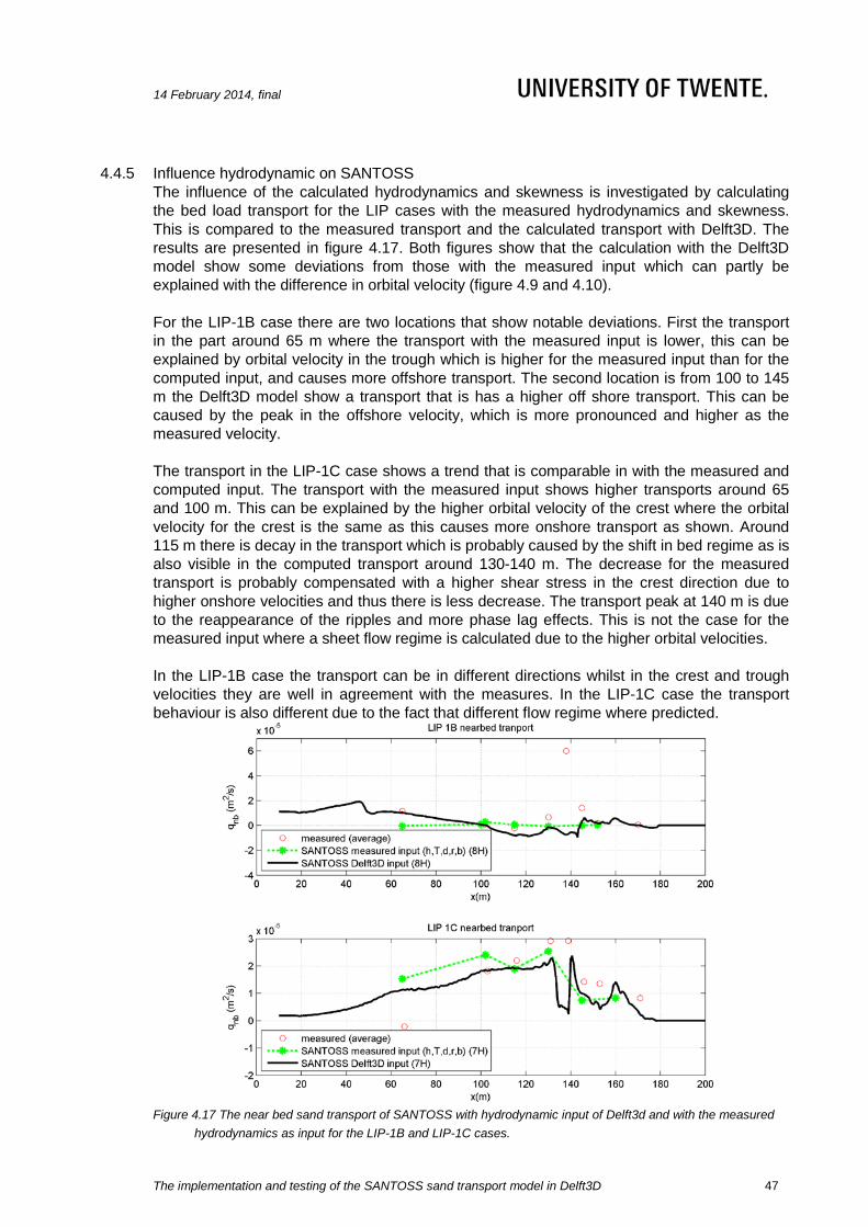
14 February 2014, final
The implementation and testing of the SANTOSS sand transport model in Delft3D
47
4.4.5 Influence hydrodynamic on SANTOSS The influence of the calculated hydrodynamics and skewness is investigated by calculating the bed load transport for the LIP cases with the measured hydrodynamics and skewness. This is compared to the measured transport and the calculated transport with Delft3D. The results are presented in figure 4.17. Both figures show that the calculation with the Delft3D model show some deviations from those with the measured input which can partly be explained with the difference in orbital velocity (figure 4.9 and 4.10). For the LIP-1B case there are two locations that show notable deviations. First the transport in the part around 65 m where the transport with the measured input is lower, this can be explained by orbital velocity in the trough which is higher for the measured input than for the computed input, and causes more offshore transport. The second location is from 100 to 145 m the Delft3D model show a transport that is has a higher off shore transport. This can be caused by the peak in the offshore velocity, which is more pronounced and higher as the measured velocity. The transport in the LIP-1C case shows a trend that is comparable in with the measured and computed input. The transport with the measured input shows higher transports around 65 and 100 m. This can be explained by the higher orbital velocity of the crest where the orbital velocity for the crest is the same as this causes more onshore transport as shown. Around 115 m there is decay in the transport which is probably caused by the shift in bed regime as is also visible in the computed transport around 130-140 m. The decrease for the measured transport is probably compensated with a higher shear stress in the crest direction due to higher onshore velocities and thus there is less decrease. The transport peak at 140 m is due to the reappearance of the ripples and more phase lag effects. This is not the case for the measured input where a sheet flow regime is calculated due to the higher orbital velocities. In the LIP-1B case the transport can be in different directions whilst in the crest and trough velocities they are well in agreement with the measures. In the LIP-1C case the transport behaviour is also different due to the fact that different flow regime where predicted.
Figure 4.17 The near bed sand transport of SANTOSS with hydrodynamic input of Delft3d and with the measured
hydrodynamics as input for the LIP-1B and LIP-1C cases.

14 February 2014, final
The implementation and testing of the SANTOSS sand transport model in Delft3D
48
In figure 4.18 the comparison is made between the calculated transports and the measured transports. When plotting the computed results against the measured results this shows the performance of the calculated transports. The erosive case, LIP-1B, shows that most of the computed results are outside the factor two lines. This indicates that with both inputs the predictions are not close to the measured transports. This goes for both Delf3D and measured hydrodynamic input and the locations on or offshore the breaker bar. The calculated transports within the factor two are calculated with the Delft3D hydrodynamic input. It should be noted that the location, for the LIP-1B case, with the least agreement (at 138 m) is not included since there was no measured skewness at that point. The accretive case, LIP-1C, shows much more agreement with the measurements. Almost all transports are within the factor two although it differs which input gives the better predictions. The on and offshore measurements are plotted, however these seem to show the same trend. In the LIP-1B case on and offshore both are mostly outside the factor two lines. In the LIP-1C both on and offshore are within the factor two lines. So the influence of a good prediction of the hydrodynamics has influence on the orbital velocities and thus the transports. Although the input of the measured hydrodynamics should be better, this does not always lead to a better prediction of the sand transport with the SANTOSS model.
Figure 4.18 Comparison between measured and computed transport rates of the hydrodynamic input with Delft3D
or form the measurements. The green markers related to the measured hydrodynamic input and the black markers related to the Delft3D hydrodynamic input. The markers as stars are offshore of the breaker bar and the plus sign for the locations onshore of the breaker bar. The solid diagonal indicates perfect agreement, the dashed lines difference of a factor two.

14 February 2014, final
The implementation and testing of the SANTOSS sand transport model in Delft3D
49
4.5 Conclusions For the assessment of the morphodynamic model Delft3D with the implemented SANTOSS sand transport model two cases of the LIP experiment are modelled, an erosive and an accretive case. The water level set up and wave height were calibrated. These were close to the measured data where the velocity profiles are quite well reproduced along the flume. The velocity profiles show that the undertow at the shallow part of the flume is overpredicted, which leads to an overestimation of the offshore sand transport. The trend in the orbital velocity is well predicted, however in the accretive case the onshore transport was underpredicted. This also showed in the velocity skewness that was well predicted in the erosive case but underpredicted in the accretive case. The acceleration skewness is well predicted in the deeper water on the other hand after the first breaker bar the computed and measured data deviate. So the calculation of the skewness and orbital velocity in the SANTOSS model are reasonable. The calculated suspended transports in the erosive case where there was a peak in offshore transport located before the breaker bars differed from the one peak in the measurements after the first breaker bar. The transport in the deeper parts is also overpredicted. In the accretive case the suspended transport is small but in the shallow part where there is some transport measured and calculated it seem to be overpredicted as well. These differences between the measured and computed suspended transport is also shown in the combination of the velocity and concentration profiles, on which the suspended transport is based. The near bed transport computed with the SANTOSS model is in line with the measurements offshore of the breaker bar for both the erosive and accretive case where the Van Rijn model (2007ab) shows an underprediction. In the shallow parts both transport models underestimate the transport in the accretive case. Whilst on the breaker bars the transport calculated with SANTOSS model shows a drastic decrease. This could be explained by the combination of the decrease in phase lag effect and the increase in offshore directed bed shear stress. In the shallow part of the erosive case both transport models show a transport in the opposite direction from the measured transport. The SANTOSS model seems to show better results with the accretive case as well as with the erosive case. The influence of the slope effect seems to be small in both cases, where the wave acceleration skewness seems to have some effect in the shallower parts of the flume. The phase lag effect is very important in the shallow parts of the flume, where the direction of the transport is influenced by the presence or absents of the phase lag effect. From the comparison of the SANTOSS model with the measured or computed hydrodynamic input two conclusions can be made. Firstly, the prediction of the hydrodynamics has influence on the orbital velocities and thus influence on the transports. Secondly, that better hydrodynamics does not always lead to better prediction of the sand transport with the SANTOSS model.

14 February 2014, final
The implementation and testing of the SANTOSS sand transport model in Delft3D
51
5 Discussion
This report provides insights in applying the SANTOSS model in the morphological model Delft3D for a near shore case. The choices that were made and the implications of the results are discussed in this chapter. The choices made in the modeling of the SANTOSS model in Delft3D are discussed in the first section and the results of the modeled LIP cases are discussed in the second section.
5.1 Conceptual additions SANTOSS The computed wave height and water level for the two LIP-cases are close to the measured data where the velocity and acceleration skewness of the waves showed some deviation. The velocity skewness was well represented in the LIP-1B case and under predicted in the LIP-1C case whereas the acceleration skewness was under predicted in the shallow parts of the flume for both cases. The velocity and acceleration skewness in the SANTOSS model are determined from the calculated hydrodynamic with the method of Ruessink et al. (2012) and Abreu et al. (2010). The parameterization is based on the relation between the ursell number and the velocity and acceleration skewness of field data. The data used to determine the relation showed quite a wide range of variation. Because of the wide range of data this entails that for any ursell number the predicted skewness has a lot of uncertainty. The parameterization can be improved by finding a parameter that could decrease this uncertainty. The slope effect on the critical shear stress added in the SANTOSS model and the slope effect on the bed load transport rates and direction was determined with the method of Bagnold (1966) which is already in Delft3D. The bed load transport is only affected by the slope effects. This is why the effect on the transport rate and direction is only applied to the bed load transport in Delft3D. With the SANTOSS model also the wave related suspended transport is included in the near bed transport. By applying the slope effects on the whole near bed transport (as is done for the SANTOSS model) it is also applied to the wave related suspended transport. This should not be done since suspended transport is not influenced by the slope effect. This could be adjusted by determining which part of the near bed transport of the SANTOSS model is wave related suspended transport. Another finding is the roughness heights calculated in the SANTOSS model. As noted in section 3.3.3 another roughness height is used to calculate the wave boundary layer because the wave boundary layer seems to be under estimated when the roughness height from the SANTOSS model is used. The roughness height in the SANTOSS, for currents and waves, model consists of two parts. The first part for the influence of the roughness related to shear stress and second the roughness related to ripples. In the ripple regime the roughness related to ripples is added to the roughness related to shear stress. The added roughness of the ripples is calculated with 0.4𝜂2/𝜆 where 𝜂 and 𝜆 are respectively the ripple height and length. The roughness effect of ripple is considerable higher than in other literature. Camenen (2009) describes the ripple related roughness with the same formula as in the SANTOSS model but the constant 0.4 can range between 5 and 40. This is a considerable influence of the ripples on the roughness which is not present in the SANTOSS model. Hereby it is not said that the calculated transport of the SANTOSS model in the ripple regime are underestimated, only that the influence of ripples is considered to be less on the roughness height in the SANTOSS model than in the literature as described by others.

14 February 2014, final
The implementation and testing of the SANTOSS sand transport model in Delft3D
52
5.2 Implementation SANTOSS in Delft3D For this research the SANTOSS model was implemented in the three dimensional model Delft3D. The SANTOSS model is a 0D model so the vertical dimension of Delft3D is not used. The SANTOSS model is based on the principal that all transport within the wave boundary layer is calculated. This research opted to use the suspended sediment transport model of Van Rijn (2007b) in combination with the SANTOSS model for the near bed transport in Delft3D. The combination, of the SANTOSS model with the suspended transport model of Van Rijn (2007b), has two issues in terms of compatibility. The first was that the wave related suspended transport is not always transported only in the wave boundary layer (Van Rijn, 2007b). This implies that if part of the wave related transport would be outside the wave boundary layer this is not calculated with the SANTOSS model. Due to the assumption that SANTOSS model includes the wave related suspended transport can lead to an underestimation of the wave related suspended transport. To overcome this problem the SANTOSS model needed to be extended with a section in which the wave related suspended transport outside the wave boundary layer could be determined. This could be done with an adjustment of the wave related suspended transport model of Van Rijn (2007ab) where the vertical integral should be from the wave boundary layer to the thickness of suspension layer near the bed. With this adjustment the same difficulties are in encountered as with the adjusting the current related suspended transport. The second issue is that the current related transport calculates the suspended transport in the water column from a reference point to the surface and not from the wave boundary layer to the surface. Although both the reference point and the wave boundary layer are in the order of a 1 to 20 centimeter these are not equal. This can lead to missing or overlapping part of the sediment transport. The current related suspended transport model of Van Rijn (2007b) was used in combination with the SANTOSS model. As described above this approach is not consistent due to the difference between the reference level and the wave boundary layer thickness. This approach was chosen because of difficulties with changing the reference height of the current related suspended transport model of Van Rijn (2007ab). The reference concentration at the reference level influences the concentration profile in two ways. Firstly, the sand concentrations in the layers below the reference level are assumed to rapidly adjust to the same concentration as the reference concentration. Secondly, the concentration in the layers above the kmx layer is determined with the advection diffusion equation which is based on the sink and source terms at the bed boundary. The sink and source are based on the reference level and concentration. By changing the reference height to the wave boundary layer thickness has the following consequences. A thicker layer near the bed is assumed to be rapidly adjusted to the reference concentration and the sink and source terms are determined with another reference height and concentration which influences the concentrations above the reference height. By changing the present reference height and concentration in the suspended model of Van Rijn (2007b) the model is used in a way that is not calibrated or validated with data which leads to uncertainty in the reliability of the constructed concentration profiles. Another approach could be to use the current method of calculating the concentration profile but changing the level at which the sink and source term are calculated.
5.3 Modeling with SANTOSS in Delft3D The sand transport results of the LIP cases in Delft3D were compared to the measured sand transports. The measured transports are not directly measured but were calculated from other measurements. The total transport is based on the integration of the mass balance equation. When assuming there is a zero transport at the beginning or end of the flume gives different results which suggests an inaccuracy in the measurement of the bed, or that sand was going out of the flume. The suspended transport is calculated from the points where a concentration

14 February 2014, final
The implementation and testing of the SANTOSS sand transport model in Delft3D
53
and velocity profile are available. The transport is an integration of the velocity times the concentration from the wave boundary layer up to the surface. The wave boundary layer was set for this to a fixed height. Since the wave boundary layer thickness changes along the flume, this method leads to uncertainty in the prediction of the suspended transport. The measured near bed transport is determined as the difference between the total and suspended transport. Therefore the inaccuracies of the total and suspended measured transport are also in the measured near bed transport. So the measured transports as used in this research should be seen as a good indication of the magnitude and direction. The modeled results show that the deeper water outside the breaker bar the predictions of the SANTOSS model are quite similar to the measured transport where in the shallower water where breaking or stronger currents occurs the results deviate more form the measured transports. This indicates that the transports offshore of the breaker bar are well predicted and onshore of the breaker bar less well predicted. This could be expected since the SANTOSS model is developed for non-breaking waves and wave dominated conditions. The velocity profiles show that the undertow in the shallower parts is overpredicted. This indicates that the suspended transport is also overpredicted because the suspended sediment is based on the multiplication of the velocity profile and the concentration profile. The undertow is also used in the SANTOSS model as currents. Due to an overprediction of the offshore related current the transport in the trough period is increased which is offshore directed and the transport in the crest is decreased which is onshore directed. So the over prediction of the undertow in shallow water leads to overprediction of the offshore suspended and near bed transport. This should be improved in the hydrodynamic part of the Delft3D. In both the LIP-1B and LIP-1C cases there is a difference between the measured near bed transport and the calculated near bed transport with the SANTOSS model at the locations of the breaker banks around 140 and 160 m. In the LIP-1B case the measurements suggest a peak in onshore transport whilst there is offshore transport computed. In the LIP-1C case the results show a decreased onshore transport. Another suggestion is that because these under estimations of the onshore transport occur on the breaker bar that they are related to the breaking of the waves. When waves break these causes turbulence witch influences the sediment transport in terms of near-bed sediment concentration levels and vertical mixing of sediment from the bed upward into the water column (Aagaard and Jensen, 2013). The SANTOSS model is not equipped with additional effects turbulence created by breaking waves, which could explain the difference between the measured and the computed near bed transports. Applying turbulence in the SANTOSS model can be done by determining the wave energy decay due to wave breaking and adding this to the dissipation due to shear stress (Roelvink and Stive, 1989) or by adding a turbulence induced motion to urms (Reniers et al., 2004). Another point is, that in the present of the phase lag effect is calculated differently for the ripple and sheet flow regime. When there is a shift of regime the calculations of the phase lag parameter also changed. In the ripple regime the phase lag parameter is calculated with the ripple height and in the sheet flow layer regime with the sheet flow layer thickness which is around a factor ten lower as the ripple height. This causes the drop in phase lag effect and thus leads to considerable changes in transport. The changes between the regimes are driven by the orbital velocity and in the ripple predictor the ripple decrease to zero for the maximum velocity of the ripple regime. So this should indicate that there is a smooth transition from the ripple height to the sheet flow layer thickness. The decay of the ripples, however, is quite quick as is shown in the top plots of figure 4.13 and 4.15. To prevent this

14 February 2014, final
The implementation and testing of the SANTOSS sand transport model in Delft3D
54
quick change in phase lag effect it may be useful to add an transition calculation between the ripple effect for the ripple and sheet flow regime.

14 February 2014, final
The implementation and testing of the SANTOSS sand transport model in Delft3D
55
6 Conclusions
The objective of this study is to improve the way Delft3D models wave-driven cross-shore sand transport by implementing the SANTOSS sand transport model. This was fulfilled by analysing how to implement the SANTOSS model in Delft3D, the implementation and analysing the sand transport results of two LIP cases that were calculated with the SANTOSS model in Delft3D. With this approach the research questions could be answered. 1 How to extent the SANTOSS model conceptually?
Three conceptual additions are made to the SANTOSS model. These additions were made so that the SANTOSS model could be implemented in Delft3D and could be applied to coastal conditions. The following additions were made: • Current dominated flow can occur in shallow water therefore the code needed to be
changed. This was done by describing the alternative skewness parameter, the sand entrained period and the dimensionless transport so that they also could be calculated if there is no crest or trough period. Another change was to prevent the crest or trough representative velocity become in the opposite direction as the peak velocity in the crest or trough period.
• In the situation that the orbital characteristics are unknown these need to be determined from other variables. The method of Ruessink et al. (2012) and Abreu et al. (2010) was used to determine the shape of one wave from the wave height, wave length and water depth. From the wave shape the wave periods, velocity and acceleration skewness were determined.
• The SANTOSS model is derived from data limited to horizontal bed conditions. In the situation that the SANTOSS model is applied to a bed with a slope the critical shear stress needs to be adapted. This was done by applying a longitudinal slope effect of Apsley and Stansby (2008) to the critical shear stress in the direction of the shear stress.
2 How should the SANTOSS model be implemented in Delft3D? For the implementation of the SANTOSS model in Delft3D the available MATLAB code is rewritten to the program code of Delft3D, FORTRAN. This was first done successfully for the stand-alone version, which was then added with the changes for strong currents. By testing the stand-alone version of SANTOSS for different skewness regimes and ranges of orbital and current velocities it showed gradual changing transports which are preferable in a numerical model. The orientation of the SANTOSS model was different from that in Delft3D. Therefore the orientation of the available input from Delft3D was transformed to the orientation in the SANTOSS model. The calculated transports with the SANTOSS model where then subsequently transformed to the orientation of Delft3D. Besides the slope effect on the critical shear stress there is also a slope effect on the transport rate and direction of the near bed sand transport. This was already in Delft3D and applied to the sand transport calculated with the SANTOS model. The method of Bagnold (1996) was used for the longitudinal slope effect and the method of Van Rijn (1993) was used for the lateral slope effect. It has to be noted that the slope effect is applied to all the sand

14 February 2014, final
The implementation and testing of the SANTOSS sand transport model in Delft3D
56
transport that was calculated with the SANTOSS model. This implies that it was also applied to the wave related suspension transport where it is normally only applied to bed load transport. The SANTOSS model accounts for both wave and current related bed transport and wave related suspended transport in the wave boundary layer. To calculate the suspended sand transport above the wave boundary layer the current related suspended transport model of Van Rijn (2007b) has been used. This model is not consistent with the near bed transport because the current related suspended transport is calculated above the reference height instead and the some wave related suspended transport can be outside the wave boundary layer. Although the compatibility is not perfect this is a good first step in using the SANTOSS model in Delft3D. 3 How does the SANTOSS model within Delft3D perform compared to the measurements
of net sand transport of a controlled wave flume experiments?
The assessment of the sediment transport of Delft3D with the implemented SANTOSS sand transport model was done by modelling two cases of the LIP experiment without morphological updating. The near bed transport was modelled with the SANTOSS model whereas the suspended transport was modelled with the Van Rijn (2007ab) model. The research used a case with wave conditions for beach erosion and a case with wave conditions for beach accretion. In the erosive case the suspended sediment was dominant whilst in the accretive case the near bed transport was dominant. The near bed transport in the erosive case shows reasonable agreement with the measurements offshore of the breaker bar. The near bed transports onshore of the breaker bar on the other hand show quite some deviation from the measurements. Where the measurements indicated a peak onshore the computed transports in contrast showed offshore transport. This appears to be due to the combination of the decrease in the phase lag effect and an increase of offshore directed bed shear stress. In the part where there were ripples the phase lag effect caused an onshore transport as measured. The suspended transport offshore of the breaker bar was overpredicted. The suspended transport onshore of the breaker bar showed a peak in offshore transport located before the breaker bars that differ from the peak in the measurements witch was after the first breaker bar. The near bed transport in the accretive case shows gradual increases of the transport with decreasing depth what was expected. One measurement at 65 m, however showed an offshore transport that was not computed. At the breaker bar the SANTOSS model showed a strong effect to the shift in bed regime and thereby underestimates the onshore transport. Overall the transport onshore of the breaker bar seems to be somewhat underestimated. This could be due to the wave related suspended transport that takes place outside the wave boundary layer. In the accretive case the suspended transport is small. At the end of the surf zone near the shore there is some measured and calculated transport. The influence of the slope effect seems to be small in both cases, whilst the wave acceleration skewness seems to have some effect in the shallower parts of the flume. The phase lag effect is very important in the shallow parts of the flume, whereas the direction of the transport is influenced by the presence or absents of the phase lag effect. From the comparison of the SANTOSS model with the measured or computed hydrodynamic input two conclusions can be made. The prediction of the hydrodynamics has influence on the orbital velocities and thus influence on the transports and that better hydrodynamics does not always lead to better prediction of the sand transport with the SANTOSS model.

14 February 2014, final
The implementation and testing of the SANTOSS sand transport model in Delft3D
57
4 How does the SANTOSS model within Delft3D perform compared to the default Van
Rijn model (2007ab)? The same suspended transport model was used in both the SANTOSS as the Van Rijn model. Therefore only the difference in the near bed transport is discussed. The near bed transport computed with the SANTOSS model agrees quite well with the measurements offshore of the breaker bar for both the erosive and accretive case whereas the Van Rijn model (2007ab) shows an underprediction of the transports. Onshore of the breaker bar the Van Rijn model (2007ab) seems to give a more accurate prediction than the SANTOSS model in the erosive case. Both models, however, do not predict the measured onshore peak transport. In the accretive case the SANTOSS model shows better agreement with the measurements than the Van Rijn model (2007ab) onshore of the breaker bar. Even though the transport calculated with the SANTOSS model shows a drastic decrease at the breaker bars which is not the case in the Van Rijn model. So the SANTOSS model seem to show better results offshore of the breaker bar than the Van Rijn model for both the erosive and accretive case. Onshore of the breaker bar the Van Rijn model shows better results for the erosive case whilst the SANTOS model shows better results for the accretive case.


14 February 2014, final
The implementation and testing of the SANTOSS sand transport model in Delft3D
59
7 Recommendations
The SANTOSS model in Delft3D can be improved by: • The method used to determine the wave orbital characteristics, velocity and
acceleration skewness and the wave periods. The calculations with the Abreu et al. (2010) and Ruessink et al. (2012) method showed some deviations from the measured data. When the cases were calculated with SANTOSS model with calculated or measured skewness data the transports differed. This indicates that there is a noticeable effect of the skewness on the transports. The parameterization of Ruessink et al. (2012) is based on quite a wide range. The wide range of data gives uncertainty in the predicted skewness. The parameterization can be improved by finding a parameter that could decrease this uncertainty.
• Changing the suspended transport model so that the suspended transport is calculated above the wave boundary layer. Currently the near bed transport by the SANTOSS model determines the transport up to the wave boundary layer height and the suspended transport is calculated above the reference height of Van Rijn (2007b). The near bed transport determines the transport below the wave boundary height and with the change in the suspended transport model it calculates the suspended transport above the wave boundary layer. When implementing the wave boundary layer in the suspended model of Van Rijn (2007b) the concentration profile should be determined with the reference height of Van Rijn (2007b) but the sink and source terms should be calculated at the wave boundary layer height. With this approach the concentration in the layer(s) between the reference height and the wave boundary layer height should be determined with a Rouse-profile as is currently done in the kmx layer.
• Implement turbulence in the SANTOSS model. At the moment the SANTOSS model calculates sand transports that deviate from the measurements where the waves to break. Since turbulence is developed when waves break and are an important factor for sand transport this might improve the predictions of the SANTOSS model under breaking waves.Applying turbulence in the SANTOSS model can be done by determining the wave energy decay due to wave breaking and adding this to the dissipation due to shear stress (Roelink and Stive, 1989). Another possibility is to add a turbulence induced motion to velocities (Reniers et al., 2004). The turbulence generated also depends on the type of breaking waves. With the classification for breaking waves proposed by Battjes (1974) different turbulence effects can be used for the different breaker types.
The following can be considered for additional research: • For a better understanding of the sand transport in the SANTOSS model additional
sensitivity analysis can be done. This to investigate the influence of different wave heights, wave periods, water depth, skewness of the waves, currents and grain sizes With this sensitivity analysis the effect on the sand transport caused by the uncertainty in the conditions can be investigated. This also provides insight into which processes are important for a good prediction with the SANTOS model. Besides the influence on the sediment transport the influence on the e.g. the wave forms can be investigated.
• The modelling of additional cases either flume experiments (e.g. Yoon and Cox, 2010) or real beach cases (e.g. Aagaard and Jensen, 2013) where high detailed data are available. With the other flume experiments the findings of the LIP cases in this

14 February 2014, final
The implementation and testing of the SANTOSS sand transport model in Delft3D
60
research can be further examined. Also the conditions could be differed, which could show some other effects as shown in the LIP cases. The modelling of real beaches with the SANTOSS model in Delft3D can provide insight in the practical application of the model where other processes, such as longshore currents, affect the sediment transport.

14 February 2014, final
The implementation and testing of the SANTOSS sand transport model in Delft3D
61
8 References
Aagaard, T. and Jensen, S. G. (2013). Sediment concentration and vertical mixing under breaking waves. Marine Geology, 336, 146-159.
Abreu, T., Silva, P. A., Sancho, F. and Temperville, A. (2010). Analytic approximate wave
form for asymmetric waves. Coastal Engineering, 57, 656-667 Apsley, D. D. and Stansby, P. K. (2008). Bed-Load Sediment Transprot on Large Slopes:
Model Formulation and Implementation within a RANS Solver. Journal of Hydraulic Engineering, 134, 1440-1451
Bagnold, R. A. (1966). An approach to the sediment transport problem from general physics,
Paper presented at Geological Survey Professional Papers, Washington, USA Battjes, J. A. (1974). Surf similarity. Proceedings of 14th Coastal Engineering conference,
American Society of Civil Engineers, New York, pp. 466-480. Battjes, J.A. and Stive, M.J.F., (1985). Calibration and verification of a dissipation model for
random breaking waves. Journal of Geophysical Research, 90, 9159-9167 Buijsrogge, R. H. (2010). SANTOSS transport model User manual. Report
SANTOSS_UT_IR4, Enschede, The Netherlands: University of Twente Camenen, B. (2009). Estimation of the wave-related ripple characteristics and induced bed
shear stress. Estuarine, Coastal and Shelf Science, 84, 553-564 Deltares (2012). Delft3D-FLOW user manual. version: 3.15.25157. Technical report, Delft,
The Netherlands: Deltares Dohmen-Janssen, C.M. (1999). Sheet flow influence on sediment transport in oscillatory
sheet flow, phase lags and mobile-bed effects, Ph.D. thesis, Delft, The Netherlands: Delft University of Technology
Dohmen-Janssen, C.M. and Hanes, D.M., (2002). Sheet flow dynamics under monochromatic
nonbreaking waves. Journal of Geophysical Research, 107, 1-21 Grant, W. D. and Madsen, O. S. (1982). Movable bed roughness in unsteady oscillatory.
Journal of Geophysical Research, 87, 469-481. Grasmeijer, B.T. (2002). Process-based cross-shore modeling of barred beaches. Ph.D.
thesis, Utrecht, The Netherlands, Utrecht University Utrecht, pp. 260 Giardino, A., Brière, C. D. E. and van der Werf, J. J. (2011). Morphological modelling of bar
dynamics with Delft3D, Report 1202345-000, Delft, The Netherlands: Deltares Hassan, W. N. M., Ribberink, J. S. (2010). Moddeling of sand transport under wave
generated sheet flow with a RANS diffusion model. Coastal Engineering, 57, 19-29

14 February 2014, final
The implementation and testing of the SANTOSS sand transport model in Delft3D
62
Isobe, M. and Horikawa, K. (1982). Study on water particle velocities of shoaling and breaking waves, Coastal Engineering, 25, 109–123
Klein Breteler, R., (2007). Wave-induced sediment transport at the small tidal inlet ‘Slufter’ of
Texel, the Netherlands. MSc. thesis, Utrecht, The Netherlands, Utrecht University Utrecht, pp. 96.
Kranenburg, W. M., Ribberink, J. S., Schretlen, J. J. L. M., Uittenbogaard, R. E. (2013). Sand
transport beneath waves: the role of progressive wave streaming and other free surface effects. Journal of Geophysical Research, 118, 122-132
Lesser, G. R., Roelvink, J. A., van Kester, J. A. T. M., and Stelling, G. S. (2004).
Development and validation of a three-dimensional morphological model. Coastal Engineering, 51, 883-915
Nielsen, P. (2006). Sheet flow sediment transport under wasves with acceleration skewness
and boundary layer streaming. Coastal Engineering, 53, 749-758 Nomden, H.G. 2011. SANTOSS sand transport model: Implementing and testing within the
morphological model UNIBEST-TC. M.Sc. thesis, Enshcede, The Netherlands, University of Twente
O’Donoghue, T., Doucette, J.S., van der Werf, J.J., Ribberink, J.S. (2006). The dimensions of
sand ripple in full-scale oscillatory flows. Coastal Engineering, 53, 997-1012. Reniers, A. J. H. M., Roelvink, J. A., and Thornton, E. B. (2004). Observations of swash zone
velocities: A note on friction coefficients. Journal of Geophysical Research-Oceans, 109 Ribberink, J. S., van der A, D. A., and Buijsrogge, R.H. (2010). SANTOSS transport model –
A new formula for sand transport under waves and currents. Report SANTOSS_UT_IR3, Enschede, The Netherlands, University of Twente
Roelvink, J. A. and Reniers, A. (1995). Lip 11d delta flume experiments – data report.
Technical report, Delft, The Netherlands, Delft Hydraulics Roelvink, J. A. and Stive, M. J. F. (1989). Bar-generating cross-shore flow mechanisms on a
beach. Journal of Geophysical Research-Oceans, 94, 4785-4800 Ruessink, B. G., Walstra, D. J. R., & Southgate, H. N. (2003). Calibration and verification of a
parametric wave model on barred beaches. Coastal Engineering, 48, 139-149 Ruessink, B. G., Ramaekers, G. and van Rijn, L. C. (2012). On the parameterization of the
free-stream non-linear wave orbital motion in nearshore morphodynamic models. Coastal Engineering, 65, 56-63
Sleath, J. F. A. (1987). Turbulent oscillatory flow over rough beds. Journal of Fluid
Mechanics, 182, 369-409 Svenden, I. A. (1984). Mass flux and undertow in a surf zone. Coastal Engineering, 8, 347-
365

14 February 2014, final
The implementation and testing of the SANTOSS sand transport model in Delft3D
63
Van der A, D. A., Ribberink, J. S., van der Werf, J. J., O’Donoghue, T., Buijsrogge, R. H., and Kranenburg, W. M. (2013). Practical sand transport formula for non-breaking waves and currents. Coastal Engineering, 76, 26-42
Van der Werf, J.J., Doucette, J.S., O'Donoghue, T., Ribberink, J.S. (2007). Detailed
measurements of velocities and suspended sand concentrations over full-scale ripples in regular oscillatory flow. Journal of Geophysical Research, 112, F02
Van der Werf, J. J., Nomden, H., Ribberink, J. S., Walstra, D. j. R., and Kranenburg, W. M.
(2012). Application of a new sand transport formula within the cross-shore morphodynamic model unibest-tc. Proceedings of the 33rd Internation Conference on Coastal Engineering, Santander, Spain
Van der Werf, J. J. (2013). Review coastal sand transport modelling in Delft3D. Delft,
Netherlands: Deltares Van Rijn, L. C. (1993). Principles of sediment transport in rivers, estuaries and coastal seas.
The Netherlands: Aqua Publications Van Rijn, L. C. (2007a). Unified view of sediment transport by currents and waves. i: Iniation
of motion, bed roughness, and bed-load transport. Journal of Hydraulic Engineering, 133, 649-667
Van Rijn, L. C. (2007b). Unified view of sediment transport by currents and waves. ii:
Suspended transport. Journal of Hydraulic Engineering, 133, 668-689 Van Rijn, L. C. (2011). Principles of fluid flow and surface waves in rivers, estuaries, seas and
oceans. The Netherlands: Aqua Publications. Wong, W. H. (2010). Master thesis: A Comparison of Practical Wave-Dominated Cross-shore
Sand Transport Models. M.Sc. thesis, Enshcede, The Netherlands, University of Twente Wright, J., Colling, A., Park, D., and Open University Oceanography Course Team. (1999).
Waves, tides and shallow-water processes (2nd ed.). Jordan Hill, Oxford: Butterworth-Heinemann.
Yoon, H. D. and Cox, D. T. (2010). Large-scale laboratory observations of wave breaking
turbulence over an evolving beach. Journal of Geophysical Research-Oceans, 115

14 February 2014, final
The implementation and testing of the SANTOSS sand transport model in Delft3D
64
List of Tables Table 2.1 Comparison of the performance of TRANSPOR2004 and SANTOSS on large
amount of sediment transport measurements (Wong, 2010). ............................ 13
Table 4.1 The initial wave conditions from Roelvink and Reniers (1995). ......................... 30
Table 4.2 Parameters settings ............................................................................................ 33

14 February 2014, final
The implementation and testing of the SANTOSS sand transport model in Delft3D
65
List of figures Figure 2.1 Terminology of the near shore zone the figure from Grasmeijer (2002). ............ 3
Figure 2.2 Schematic illustration of the wave forms approaching the shore (Grasmeijer, 2002). .................................................................................................................... 3
Figure 2.3 Change of orbital motion under waves approaching the shore (Grasmeijer, 2002). .................................................................................................................... 4
Figure 2.4 The interactions between the different models of Delft3D. .................................. 6
Figure 2.5 Example of a vertical grid consisting of six equal thickness σ-layers (left), definition of 𝜎, 𝜉,ℎ 𝑎𝑛𝑑 𝑧 (right) (Deltares, 2012). ................................................. 7
Figure 2.6 Schematic arrangement of flux bottom boundary conditions (Deltares, 2012). 10
Figure 2.7 Approximation of concentration and concentration gradient at bottom of kmx layer (Deltares, 2012). ........................................................................................ 11
Figure 2.8 Definition sketch of the velocity time series in wave direction (Ribberink et al., 2010). .................................................................................................................. 13
Figure 3.1 Definition sketch of the velocity time series in wave direction (Ribberink et al., 2010). .................................................................................................................. 18
Figure 3.2 Calculation of non-dimensional transport as a function of root mean square orbital velocity (Urms) for fine and medium sand. For all calculations the wave period T=6.5s and the water depth h=3.5m and in cases c1-d2 there are progressing surface wave effects. ...................................................................... 23
Figure 3.3 Calculation of non-dimensional transport as a function of current (Unet) for fine and medium sand. For all calculations the wave period T=6.5s, the water depth h=3.5m, the root mean square of the orbital velocity Urms=0.65 m/s and in cases c1-d2 there are progressing surface wave effects. ............................................ 24
Figure 3.4 The orientation of the grid of Delft3D model in relation to the grid of SANTOSS model. ................................................................................................................. 25
Figure 4.1 Schematic presentation of the LIP experiment (Roelvink and Reniers, 1995). . 29
Figure 4.2 Location of the fixed measuring tools EMS for velocities and PS for surface water elevation (Roelvink and Reniers, 1995) ................................................... 30
Figure 4.3 Horizontal (top) and vertical (bottom) grids as used in Delft3D. Only separation of δ-layers is shown in vertical grid. ................................................................... 31
Figure 4.4 Three step calibration procedure. ...................................................................... 32
Figure 4.5 Bottom profile, water level setup and representative wave height of the LIP-1B calibration case at 8 hours. ................................................................................ 33
Figure 4.6 Velocity and concentration profiles along the flume of the LIP-1B calibration case at 8 hours. .................................................................................................. 34
Figure 4.7 Bottom profile, water level setup and representative wave height of the LIP-1C calibration case at 7 hours. ................................................................................ 34
Figure 4.8 Velocity and concentration profiles along the flume of the LIP-1C calibration case at 7 hours. .................................................................................................. 35
Figure 4.9 The on- and offshore orbital velocities, velocity and acceleration skewness of the LIP-1B case. ................................................................................................. 36

14 February 2014, final
The implementation and testing of the SANTOSS sand transport model in Delft3D
66
Figure 4.10 The on- and offshore orbital velocities, velocity and acceleration skewness of the LIP-1C case. ................................................................................................. 36
Figure 4.11 The first graph is the interpolated velocity profile, the second figure is the fitted rouge profile through the concentration measurements and the third figure is the profile of the velocity times the concentration. ................................................... 38
Figure 4.12 The top plot gives the measured bottom profiles at the beginning and end of the LIP-1B case. The second, third and fourth plot give respectively the near bed, suspended and total transport. In these three plots the red markers and line are for the measured transport, the blue lines are the transport calculated with the Van Rijn model (2007ab and the black lines are the transports calculated with the SANTOSS model. The solid lines related to the beginning (0H) and the dashed lines to the end (16H) of the LIP-1B case. ............................................ 40
Figure 4.13 The plots above show the processes calculated within the SANTOSS model for the LIP-1B case. The top plot provides the ripple height, the second plot the shields stress, the third plot the representative velocities in the crest and trough period, the fourth plot the representative shear stress in the crest and trough period, the fifth plot the critical shear stress in the trough and crest period and the last plot the phase lag parameter for the crest and trough period. .............. 41
Figure 4.14 The top plot gives the measured bottom profiles at the beginning and end of the LIP-1C case. The second, third and fourth plot give respectively the near bed, suspended and total transport. In these three plots the red markers and line are for the measured transport, the blue lines are the transport calculated with the Van Rijn model (2007ab and the black lines are the transports calculated with the SANTOSS model. The solid lines related to the beginning (0H) and the dashed lines to the end (13H) of the LIP-1C case ............................................. 44
Figure 4.15 The plots above show the processes calculated within the SANTOSS model for the LIP-1B case. The top plot provides the ripple height, the second plot the shields stress, the third plot the representative velocities in the crest and trough period, the fourth plot the representative shear stress in the crest and trough period, the fifth plot the critical shear stress in the trough and crest period and the last plot the phase lag parameter for the crest and trough period. .............. 45
Figure 4.16 The near bed transport with the SANTOSS model for the LIP-1B and LIP-1C case calculated without phase lag, slope and acceleration skewness. ............. 46
Figure 4.17 The near bed sand transport of SANTOSS with hydrodynamic input of Delft3d and with the measured hydrodynamics as input for the LIP-1B and LIP-1C cases. .................................................................................................................. 47
Figure 4.18 Comparison between measured and computed transport rates of the hydrodynamic input with Delft3D or form the measurements. The green markers related to the measured hydrodynamic input and the black markers related to the Delft3D hydrodynamic input. The markers as stars are offshore of the breaker bar and the plus sign for the locations onshore of the breaker bar. The solid diagonal indicates perfect agreement, the dashed lines difference of a factor two............................................................................................................. 48
Figure B.1 Example of the relation of parameters r and 𝝓 of the expression of Abreu et al. (2010) in relation to the acceleration and velocity skewness. ............................ IV
Figure B.2 Relation between the total non-linearity B and the nonlinear parameter r and the basic fitted of that relation. ................................................................................... V

14 February 2014, final
The implementation and testing of the SANTOSS sand transport model in Delft3D
67
Figure C.1 The relation between the SANTOSS codes in Delft3D. ...................................... VI
Figure D.1 The top figure shows the magnitude of the modelled orbital velocities with the black (crest) and bleu (trough) lines, the magnitude of the measured orbital velocities are the red boxes for the crest and the triangles for the trough. The purple line represents the magnitude of the current velocity at the top of the wave boundary layer which height is presented in the bottom figure. (LIP-1B case). .................................................................................................................... X
Figure D.2 The top figure shows the ripple height, the second figure represents the Shields stress of the wave and current combined and the third figure shows the current related roughness height with the blue line and the wave related roughness height with the black line. (LIP-1B case). ............................................................. X
Figure D.3 The top figure shows the representative wave-current velocities, the middle figure shows the wave-current friction factor and the bottom figure shows the representative bed shear stress. In all the figures the crest period is shown with the black lines and for the trough period is shown with the blue lines. (LIP-1B case). ................................................................................................................... XI
Figure D.4 The top figure shows the phase lag parameter for the wave crest with the black line and the wave trough with the blue line. The red line is the threshold for exchange between the half cycles. The middle figure represents the load components that are transported in the crest period where the black line represents the load that is suspended in the crest period and the blue line the load that is suspended in the trough period. The bottom figure represents the load components that are transported in the trough period where the black line represents the load that is suspended in the crest period and the blue line the load that is suspended in the trough period. (LIP-1B case). ............................... XI
Figure D.5 The top figure represents the duration of the crest half cycle with the black line and the trough half cycle with the blue line. The middle figure presents the dimensionless transport for the crest half cycle with the black line and the trough half cycle with the blue line. The bottom figure represents the transport calculated with the SANTOSS model in the direction of the wave. (LIP-1B) ..... XII
Figure D.6 The top figure shows the magnitude of the modelled orbital velocities with the black (crest) and bleu (trough) lines, the magnitude of the measured orbital velocities are the red boxes for the crest and the triangles for the trough. The purple line represents the magnitude of the current velocity at the top of the wave boundary layer which height is presented in the bottom figure. (LIP-1B case). .................................................................................................................. XII
Figure D.7 The top figure shows the ripple height, the second figure represents the Shields stress of the wave and current combined and the third figure shows the current related roughness height with the blue line and the wave related roughness height with the black line. (LIP-1B case). .......................................................... XIII
Figure D.8 The top figure shows the phase lag parameter for the wave crest with the black line and the wave trough with the blue line. The red line is the threshold for exchange between the half cycles. The middle figure represents the load components that are transported in the crest period where the black line represents the load that is suspended in the crest period and the blue line the load that is suspended in the trough period. The bottom figure represents the load components that are transported in the trough period where the black line represents the load that is suspended in the crest period and the blue line the load that is suspended in the trough period. (LIP-1C case). ............................ XIII

14 February 2014, final
The implementation and testing of the SANTOSS sand transport model in Delft3D
68
Figure D.9 The top figure shows the representative wave-current velocities, the middle figure shows the wave-current friction factor and the bottom figure shows the representative bed shear stress. In all the figures the crest period is shown with the black lines and for the trough period is shown with the blue lines. (LIP-1C case). ................................................................................................................ XIV
Figure D.10 The top figure shows the magnitude of the modelled orbital velocities with the black (crest) and bleu (trough) lines, the magnitude of the measured orbital velocities are the red boxes for the crest and the triangles for the trough. The purple line represents the magnitude of the current velocity at the top of the wave boundary layer which height is presented in the bottom figure. (LIP-1C case). ................................................................................................................ XIV

14 February 2014, final
The implementation and testing of the SANTOSS sand transport model in Delft3D
I
A Calibration parameters roller model
The roller dissipation coefficient, αrol (Alfaro), is a first order constant that effects the wave energy dissipation due to breaking waves. Due to the dissipation the wave energy and wave height decrease. The coefficient αrol affect the wave height in the locations where the waves break; the higher αrol the lower the wave height. The effect of αrol on the wave height is given in equation 4.1, 4.2 and 4.3. The short wave energy, Ew, is as follows:
𝐸𝑤 =18𝜌𝑤𝑔𝐻𝑟𝑚𝑠
2
A.1
Where 𝜌𝑤 is the water density, g is the acceleration due to gravity and Hrms is the root-mean-square of the wave height. The wave energy is determined with the following balance equation:
𝜕𝐸𝑤𝜕𝑡
+𝜕𝜕𝑥
�𝐸𝑤𝑐𝑔 cos𝜃�+𝜕𝜕𝑦
�𝐸𝑤𝑐𝑔 sin𝜃� = −𝐷𝑤 −𝐷𝑓
A.2
Where cg is the wave group velocity, θ is the wave angle from the shore normal, and Dw and Df are the dissipation terms due to breaking and bottom friction. The dissipation due to breaking waves is described as follows:
𝐷𝑤 =14αrol𝜌𝑤𝑔𝑓𝑝 exp�−
𝐻𝑚𝑎𝑥2
𝐻𝑟𝑚𝑠2 � (𝐻𝑚𝑎𝑥2 + 𝐻𝑟𝑚𝑠
2 )
A.3
Where αrol is the dissipation coefficient, fp is the spectral peak frequency and Hmax is the maximal wave height. The parameter αrol has an advised range from 0.5 to 1.2 and the default value is 1.0. The maximum wave height is defined as follows:
𝐻𝑚𝑎𝑥 =0.88𝑘
tanh �𝛾𝑤
0.88𝑘ℎ𝑟𝑒𝑓�
A.4
Where k is the wave number, href is the water depth, γw is the wave breaking index. The wave breaking index is a parameter that limits the wave height as a function of the water depth. This can be set with a constant value or computed by the expression of Battjes & Stive (1995) or Ruessink et al. (2003). With a low wave breaking index there is an increase of waves breaking on the outer bar what gives a flattening of that bar. The parameter αrol has an advised range from 0.5 to 0.8 and respectively -2 and -1 for the computed expressions. The default setting is a constant value of 0.55. It takes waves around one wave length to start and stop breaking. This phenomenon is accounted for in Delft3D amongst others by using a weighted average at a certain distance seaward of the water depth �ℎ𝑎𝑣𝑔� instead of a local water depth �ℎ𝑟𝑒𝑓� in equation 4.4. In morphological modeling this method is most frequently used. The user defined breaker delay parameter (Flam) is the length in wavelengths that is being used for the averaging of the water depth in seaward direction. Assuming an increase in water depth in seaward direction then the increase of Flam causes an increase in the maximum wave height. The parameter Flam has an advised range from -3 to 0 and the default value is 0. The energy that is dissipated due to the friction of the bottom is determined as follows;

14 February 2014, final
The implementation and testing of the SANTOSS sand transport model in Delft3D
II
𝐷𝑓 = 𝑓𝑤
𝜌𝑤√𝜋
𝑢𝑜𝑟𝑏3
A.5
The dissipation is calibrated with the bottom friction factor (𝑓𝑤). With an increase of the bottom friction factor there is more energy dissipated which causes a decrease in wave height. This has more effect in shallower water due to the higher orbital velocities near the bed. The parameter 𝑓𝑤 has an advised range from 0 to 0.3 and the default value is 0. The slope of the wave front is important in the roller energy balance. The roller determines the rate of wave energy that is transferred from the roller to the roller in the water layer below. The dissipation of roller energy (𝐷𝑟) is related to the slope of the wave front as follows;
𝐷𝑟 = 2𝛽𝑟𝑜𝑙𝑔
𝐸𝑟𝑐𝑝ℎ
A.6
Where the roller slope parameter is 𝛽𝑟𝑜𝑙 and 𝑐𝑝ℎ is the phase celerity. The roller energy dissipation is related to the wave energy dissipation in the following way;
𝜕𝐸𝑟𝜕𝑡
+𝜕𝜕𝑥
�2𝐸𝑟𝑐𝑝ℎ cos𝜃�+𝜕𝜕𝑦
�2𝐸𝑟𝑐𝑝ℎ sin𝜃� = 𝐷𝑤 − 𝐷𝑟
A.7
The influence of the roller slope parameter on the wave height is small but this parameter can be used to calibrate the water level setup and the currents in the cross-shore direction. The parameter 𝛽𝑟𝑜𝑙has and advised range from 0.03 to 0.20 and the default value is 0.05.

14 February 2014, final
The implementation and testing of the SANTOSS sand transport model in Delft3D
III
B Approximation wave form for skewed waves
The analytical expression of Abreu et al. (2010) provides a representation of both velocity and acceleration skewness that is found in shallow water waves. The analytical expression for the orbital velocities is defined as follows:
𝑈(𝑡) = 𝑈𝑤𝑓�sin(𝜔𝑡) + 𝑟 sin𝜙
1 + √1 − 𝑟2�
[1− 𝑟 cos(𝜔𝑡 + 𝜙)]
B.1
where Uw represents the orbital velocity amplitude, ω=2π/T where ω is the angular frequency and T is the wave peak period, 𝜙 is the waveform parameter (−π ≤ 𝜙 ≤ 0), r is the parameter of skewness or nonlinearity (−1 < 𝑟 ≤ 1) and 𝑓 is the dimensionless factor as a function of r �𝑓 = √1 − 𝑟2�. The acceleration corresponding with the velocity time series is given by:
𝑎(𝑡) = 𝑈𝑤𝜔𝑓cos(𝜔𝑡)− 𝑟 cos𝜙 − 𝑟2
1 + √1− 𝑟2sin𝜙 sin(𝜔𝑡 + 𝜙)
[1 − 𝑟 cos(𝜔𝑡 + 𝜙)]2
B.2
The graphs in figure 3.4 show the effect of the parameters on the wave form. Where the parameter r is positive the waves are positive velocity skewed and if the parameter r is negative the waves are negative velocity skewed. The velocity skewness is a measure of the maximum velocity and the minimum velocity which is described by:
𝑅 =𝑈𝑚𝑎𝑥
𝑈𝑚𝑎𝑥 − 𝑈𝑚𝑖𝑛
B.3
Depending on parameter 𝜙 the wave is backward or forward leaning, which is a measure of the acceleration skewness. A backward leaning wave has a larger acceleration period as a deceleration period and a forward leaning wave has a larger deceleration period as an acceleration period. This measure of acceleration skewness is described by:
β =
𝑎𝑚𝑎𝑥
𝑎𝑚𝑎𝑥 − 𝑎𝑚𝑖𝑛
B.4
Ruessink et al. (2012) present a parameterization for the nonlinear parameters r (index of skewness or non-linearity) and 𝜙 (waveform parameter) that are used in the equations of Abreu et al. (2010) to estimate the skewed-asymmetric shape of the near bed orbital motion. These parameters are estimated from the values of the significant wave height (Hs), wave period (T) and water depth (h). In four steps the Ursell number, which is a function of Hs, T and h, is related to the nonlinear parameters r and 𝜙. First the Ursell number is related to the wave skewness (Su) and the wave asymmetry (Au). Secondly the wave skewness and wave asymmetry are related to the total non-linearity (B) and the phase(𝜓). Thirdly the total non-linearity and the phase are related to the Ursell number. Finally the total non-linearity and the phase are related to the nonlinear parameters r and 𝜙 witch are then also related to the Ursell number and thus the three variables Hs, T and h.
−𝛑 < 𝜙 < −𝟎.𝟓𝛑 −𝟎.𝟓𝛑 < 𝜙 < 𝟎

14 February 2014, final
The implementation and testing of the SANTOSS sand transport model in Delft3D
IV
( 𝟎<
𝑟<𝟏)
Positive velocity skewed (Su>0, R>0.5) Backward leaning (Au>0, β<0.5)
Positive velocity skewed (Su>0, R>0.5) Forward leaning (Au<0, β>0.5)
( −𝟏
< 𝑟
<0)
Negative velocity skewed (Su<0, R<0.5) Forward leaning (Au<0, β>0.5)
Negative velocity skewed (Su<0, R<0.5) Backward leaning (Au>0, β<0.5)
Figure B.1 Example of the relation of parameters r and 𝝓 of the expression of Abreu et al. (2010) in relation to the
acceleration and velocity skewness. The wave skewness (Su) and the wave asymmetry (Au) is related to the Ursell number from field data The wave skewness and asymmetry are described by:
𝑆𝑢 = 𝑈𝑤����
3
𝜎𝑈𝑤3 , 𝐴𝑢 = 𝐻(𝑈𝑤����)3
𝜎𝑈𝑤3
B.5
where Uw is the velocity amplitude, 𝜎𝑈𝑤 is the standard deviation of Uw and H(Uw) is the Hilbert transform of Uw. The Ursell number is described by:
𝑈𝑟 =34𝑎𝑤𝑘
(𝑘𝑑)3
B.6
where aw=0.5Hs, k is the local wave number computed with linear wave theory using wave peak period (T) and the water depth (d). To determine k the wave number is k=2π/L with wave length 𝐿 = �𝑔ℎ𝑇. From data used by Ruessink et al. (2012) a positive relation between Su and Ur is determined this indicates that the waves have a larger wave crest period as trough period and a negative relation between Au and Ur what indicates a forward leaning wave. The measurements of Su and Au were combined into a measure of total (non-dimensional) non-linearity
𝐵 = �𝑆𝑢2 + 𝐴𝑢2
B.7
and phase
𝜓 = tan−1 𝐴𝑢/𝑆𝑢
B.8

14 February 2014, final
The implementation and testing of the SANTOSS sand transport model in Delft3D
V
Implying that 𝑆𝑢 = 𝐵 cos𝜓 and 𝐴𝑢 = 𝐵 sin𝜓. The total non-linearity B and the phase 𝜓 depends on Su and Au and thus on the Ursell number. Ruessink et al. (2012) suggest a fit between B and Ur in the form of a Boltzman sigmuoid function and between 𝜓 and Ur in the form of a tanh-function. The total non-linearity can be written as follows:
𝐵 =0.857
1 + exp �−0.471− log𝑈𝑟0.297 �
B.9
and the phase as:
𝜓 = −90𝜊 + 90𝜊tanh �0.815/𝑈𝑟0.672�
B.10
Next B and 𝜓 are related to the parameters, r and 𝜙, of the analytical expression of Abreu et al. (2010). The B is related to r as (Malarkey and Davies, 2012):
𝐵 =
3𝑏
�2(1− 𝑏2) 𝑤𝑖𝑡ℎ 𝑏 =
𝑟�1 + √1 − 𝑟2�
B.11
and the phase is related to 𝜙 as:
𝜙 = −𝜓 − 𝜋/2. B.12
It is difficult to get parameter r from a given B with equation 2.13. To find the relation between B and r, so that r can be determined form B, these are plotted in figure 5. By basic fitting a third order polygon is determined in the part of positive r to find the relation between r and B. This function is as follows:
𝑟 = 0.0517𝐵3 – 0.4095𝐵2 + 1.0853𝐵 – 0.0099 𝑤𝑖𝑡ℎ
𝐵 = �𝑆𝑢2 + 𝐴𝑢2
B.13
The fitted relation is only fitted in the rage of a positive r so the relation is only for the cases that 0<r<1. In the cases with a positive r the waves are skewed positive. Figure 3.5 also shows that the r is negative if 𝜙 is between 0 and -0.5π and if the asymmetry parameter Au is greater as zero or if 𝜙 is between -0.5π and –π and the asymmetry parameter Au is smaller as zero. So in those cases the calculated parameter r=-r. This can be done because of the symmetry of the relation between r and B for positive and negative r values.
Figure B.2 Relation between the total non-linearity B and the nonlinear parameter r and the basic fitted of that
relation.
y = 0,0517x3 - 0,4095x2 + 1,0853x - 0,0099 R² = 0,9998
-1
-0,5
0
0,5
1
0 0,5 1 1,5 2 2,5
r
B
r against B
Poly. (r against B)

14 February 2014, final
The implementation and testing of the SANTOSS sand transport model in Delft3D
VI
C Description FORTRAN codes
In this section the different FORTRAN files of the SANTOSS model within Delft3D are described. The discretion contains the important functions, the in- and output of the files and the relation between the files. The SANTOSS model consists of 10 scripts, namely: santoss.f90, santoss_RRR12.for, santoss_abreu.for, santoss_orb.for, santoss_ripple.for, santoss_bss1.for, santoss_bss2.for, santoss_bsscurrent.for, santoss_sfltD99.for and santoss_core.for. The way they are in Delf3D is given schematically in the figure C.1.
Figure C.1 The relation between the SANTOSS codes in Delft3D. santoss.f90 This is the main script of the SANTOSS function that calls the other scripts for prepossessing the input so that can be used in the SANTOSS formula. The steps that are made in this script are shortly described. • Pre-processing of the orientation. The orientation of the SANTOSS model and Delft3D
differ. The angle between the waves and the current is needed in the SANTOSS model. By defining the angle of the current and the angle of the wave with the x-axis and, the angle between the two can be determined.

14 February 2014, final
The implementation and testing of the SANTOSS sand transport model in Delft3D
VII
• Calculating the parameterisation for the wave form. Because the skewness of the wave is not available as input for the SANTOSS model this is calculated for the wave height, water depth and wave length. This is done using the parameterisation of Ruessink et al. (2012) what is programed in santoss_RRR12.for.
• Calculating the wave form. From the parameterisation of Ruessink et al. (2012) the wave form, including the skewness, can be determined by analytical approximation of Abreu et al. (2010) that gives time series of the velocities during one wave period. This is programed in santoss_abreu.for.
• Calculating partial wave trough and crest periods. From the time series of the wave form the periods of a wave as described for the SANTOSS model can be determined by the zero crossing and the maximum and minimum velocities. This also gives the needed skewness parameters r and β that the SANTOSS model needs as input. First this is done for the wave time series without current velocity and in the case that the is a current velocity the min and max velocity and the periods are calculated again with the combined wave and current velocity. This is programed in santoss_orb.for.
• Calculating the ripple height and length. The ripple height and length can be estimated with the method by O’Donoghue et al. (2006) that is programmed in santoss_ripple.for.
• Calculating the bed shear stress. The bed shear stress is determined with the santoss_bss2.for what need the roughness height and friction factor as input. These are determined with santoss_bss1.for. The script santoss_bss1.for also determines the partial the velocity on top of a given wave boundary layer height. In the case that there are no waves and thus no orbital velocities the bed shear stress is calculated with santoss_bsscurrent.for that only calculates the bed shear stress caused by current related flow.
• Calculating the sheet flow layer thickness. The sheet flow layer is determined with the method by Dohmen-Janssen (1999) that is programmed in santoss_sfltD99.for. The sheet flow layer thickness is calculated differently for only waves and both waves and a current.
• Calculating the critical bed shear stress and fall velocity. The critical bed shear stress and the fall velocity are determined with the method described by Soulsby (1997). These are determined in the script santoss.f90
• Calculating the transport rates. With the preprocessing of the input in the previous steps the transport rates are determined with the SANTOSS formula that is programmed in santos_core.for. The script gives the transport rates in the direction in the x and y directions of the SANTOSS formula where the x direction is in the propagation direction of the waves and the y direction is perpendicular to the x direction.
With the keys different effects can be turned off. The SL_EFFECTS is the slope effect on the critical shear stress, the SW_EFFECTS is the effect of progressive surface waves, the AS_EFFECTS are the effects of an acceleration skewness in a wave and the PI_EFFECTS gives the possibility that there is exchange of sediment transport between the two half cycles of a wave. Input Output d, D50, D90, hrms, tp, uorb, teta, uuu, vvv, umod, zumod, ag, vicmol, rhosol, rhowat, dzduu, dzdvv KEYS: SL_EFFECTS, SW_EFFECTS, AS_EFFECTS, PL_EFFECTS
Qsx, Qsy

14 February 2014, final
The implementation and testing of the SANTOSS sand transport model in Delft3D
VIII
santoss_RRR12.for In this script the parameter that are needed for the santoss_abreu.for are calculated for the wave height, water depth and wave length. This is done with the paratmeterisation developed by Ruessink et al. (2012). Input Output pi, ag, hw, tp, d Sk, As, phi_AB, r_AB
santoss_abreu.for In this script a time series is calculated of the velocities during one wave period. This is done by with the analytical approximation of Abreu et al. (2010). The script gives as output 200 time steps over the period of one wave. Input Output phi_AB, r_AB, Urms, tp, pi nt, tw, Uorb_time_serie
santoss_orb.for This script uses the otbital time series and the current velocity (if present) to determine the orbital period, the maximum wave crest and trough velocities and the representative velocities. Also the velocities for the wave and current combined are determined. Input Output Tw, Uorb_time_serie, Unet, ang, pi, tp, nt Tc, Tcu, Tcd, Tt, Ttu, Ttd, uw, ut , uc ,uwc,
uwt, ucy, ucx, uwcrepr, uwtrepr, ucxrepr, ucyrepr, ucrepr, utrepr, aw
santoss_ripple.for In this script the ripple height and length are estimated with the method by O’Donoghue et al. (2006). The ripples are estimated based on the median grain size and the maximum and minimum orbital velocity. Input Output D50, uwc, uwt, Delta, g, pi, aw Rh, Rl
santoss_bss1.for This script is first used to determine de velocity on top of the wave boundary layer. This is then used in the santoss_orb.for. Then when the wave and current combined velocities are determined this script is used to determine the current and wave related roughness and the fiction factors related to the current, wave and the combined current and waves. Input Output ag, d, D50, D90, Delta, aw, uw, pi, Unet, Zref, Rh, Rl, uw, ut, uc, ut , ang,
Theta, ksw, ksc, fc, fw,fcw, unet_delwblt, alpha, delwblt
santoss_bss2.for In this script the (representative) bed shear stress is determined based on the current and wave related velocities, roughness heights and friction factors. This calculated bed shear stress also depends on is the surface wave effect and wave acceleration skewness is included. Therefor two keys are available in this script to determine if these effects should be included in the calculated bed shear stress. The key of the surface wave effect is

14 February 2014, final
The implementation and testing of the SANTOSS sand transport model in Delft3D
IX
SW_EFFECTS and for the wave acceleration skewness is AS_EFFECTS. If the key is set to ‘0’ the effect is not included and if it is ‘1’ it is included. Input Output pi, ag, d, rhowat, rhosol, Delta, D50, D90, b, r, tp, unet_delwblt, Ang, delwblt, Rh, Rl, uwc(repr), uwt(repr), ucx(repr), ucy(repr), uc(repr), ut(repr), aw, ksw, ksc, fc, fw,fcw, unet_delwblt, alpha, delwblt KEYS: SW_EFFECTS, AS_EFFECTS
Sc(repr), St(repr), Swc(repr), Swt(repr), Scx(repr), Scy(repr), Stx(repr), Sty(repr)
santoss_bsscurrent.for In this code the bed roughness, friction factor and bed shear stress are determined only for currents. Also the effect of acceleration skewness and surface wave propagation is not present due to the absent of waves. Input unet_delwblt, alpha, delwblt pi, ag, d, rhowat, rhosol, Delta, D50, D90, unet_delwblt, Ang, Zref, delwblt, Rh, Rl
unet_delwblt, alpha, delwblt, Sc, Scx, Scy
santoss_sfltD99.for In this script the sheet flow layer thickness is calculated by using the method of Dohmen-Jansen (1999). There the sheet flow layer is based only on waves (SFLT_W_C=’w’) or on waves and a current (SFLT_W_C=’wc’). Input Output D50, Sc, Sc_sflt, St_sflt, Swc_sflt KEYS: SFLT_W_C, GRAD
SFLTc, SFLTt,
santoss_core.for In this script the SANTOSS formula is executed. First the phase lag parameters are determined where the maximum vertical orbital velocity is calculated for real waves. Secondly the load entrained components and the transport components are calculated. There are two effect that can be turned on and off in this script. The first is the effect of surface waves on the settling velocity, the key is SW_EFFECTS. The second is the phase lag effect that allows exchange of transport between the two half cycles, the key is PL_EFFECTS. If the key is set to ‘0’ the effect is not included and if it is ‘1’ it is included. Input Output pi, ag, D50, d, hw, rhosol, rhowat, Delta, r, b, tp, Tc, Tt, Tcu, Tcd, Ttu, Ttd, SFLTc, SFLTt, wss, Rh, Scr_c, Scr_t, Screpr, Strper, Scxrepr, Scyrepr, Stxrepr, Styrepr, uwt, uwc, n, m, alphas, alphar, Pcr KEYS: SW_EFFECTS,PL_EFFECTS
Pc, Pt, Oc, Occ, Oct, Ot, Ott, Otc, Qsx, Qsy

14 February 2014, final
The implementation and testing of the SANTOSS sand transport model in Delft3D
X
D Results processes within the SANTOSS model
This appendix shows figures of the processes within the SANTOSS model for the LIP-1B and LIP-1C case. LIP-1B
Figure D.1 The top figure shows the magnitude of the modelled orbital velocities with the black (crest) and bleu
(trough) lines, the magnitude of the measured orbital velocities are the red boxes for the crest and the triangles for the trough. The purple line represents the magnitude of the current velocity at the top of the wave boundary layer which height is presented in the bottom figure. (LIP-1B case).
Figure D.2 The top figure shows the ripple height, the second figure represents the Shields stress of the wave and
current combined and the third figure shows the current related roughness height with the blue line and the wave related roughness height with the black line. (LIP-1B case).

14 February 2014, final
The implementation and testing of the SANTOSS sand transport model in Delft3D
XI
Figure D.3 The top figure shows the representative wave-current velocities, the middle figure shows the wave-
current friction factor and the bottom figure shows the representative bed shear stress. In all the figures the crest period is shown with the black lines and for the trough period is shown with the blue lines. (LIP-1B case).
Figure D.4 The top figure shows the phase lag parameter for the wave crest with the black line and the wave
trough with the blue line. The red line is the threshold for exchange between the half cycles. The middle figure represents the load components that are transported in the crest period where the black line represents the load that is suspended in the crest period and the blue line the load that is suspended in the trough period. The bottom figure represents the load components that are transported in the trough period where the black line represents the load that is suspended in the crest period and the blue line the load that is suspended in the trough period. (LIP-1B case).

14 February 2014, final
The implementation and testing of the SANTOSS sand transport model in Delft3D
XII
Figure D.5 The top figure represents the duration of the crest half cycle with the black line and the trough half cycle
with the blue line. The middle figure presents the dimensionless transport for the crest half cycle with the black line and the trough half cycle with the blue line. The bottom figure represents the transport calculated with the SANTOSS model in the direction of the wave. (LIP-1B)
LIP-1C
Figure D.6 The top figure shows the magnitude of the modelled orbital velocities with the black (crest) and bleu
(trough) lines, the magnitude of the measured orbital velocities are the red boxes for the crest and the triangles for the trough. The purple line represents the magnitude of the current velocity at the top of the wave boundary layer which height is presented in the bottom figure. (LIP-1B case).

14 February 2014, final
The implementation and testing of the SANTOSS sand transport model in Delft3D
XIII
Figure D.7 The top figure shows the ripple height, the second figure represents the Shields stress of the wave and
current combined and the third figure shows the current related roughness height with the blue line and the wave related roughness height with the black line. (LIP-1B case).
Figure D.8 The top figure shows the phase lag parameter for the wave crest with the black line and the wave
trough with the blue line. The red line is the threshold for exchange between the half cycles. The middle figure represents the load components that are transported in the crest period where the black line represents the load that is suspended in the crest period and the blue line the load that is suspended in the trough period. The bottom figure represents the load components that are transported in the trough period where the black line represents the load that is suspended in the crest period and the blue line the load that is suspended in the trough period. (LIP-1C case).

14 February 2014, final
The implementation and testing of the SANTOSS sand transport model in Delft3D
XIV
Figure D.9 The top figure shows the representative wave-current velocities, the middle figure shows the wave-
current friction factor and the bottom figure shows the representative bed shear stress. In all the figures the crest period is shown with the black lines and for the trough period is shown with the blue lines. (LIP-1C case).
Figure D.10 The top figure shows the magnitude of the modelled orbital velocities with the black (crest) and bleu
(trough) lines, the magnitude of the measured orbital velocities are the red boxes for the crest and the triangles for the trough. The purple line represents the magnitude of the current velocity at the top of the wave boundary layer which height is presented in the bottom figure. (LIP-1C case).