the impact of traffic images on route choice and …ceprofs.tamu.edu/mburris/papers/impact of...

The Impact of Traffic Images on Route Choice and Value of Time Estimates in Stated-

Preference Surveys

Carl E. Harline

Alliance Transportation Group

11500 Metric Blvd., Building M-1, Suite 150

Austin, TX 78758

512-821-2085

[email protected]

Dr. Mark W. Burris, Ph.D.

Texas A&M University

CE/TTI Room 301B

3136 Texas A&M University

College Station, TX 77843

979-845-6481

[email protected]

5,704 words + 2 figures + 5 tables

February 28, 2014

Harline and Burris 2

ABSTRACT A difficult aspect of using stated-preference experiments to predict travel behavior is properly

presenting attributes and characteristics of hypothetical trips to respondents. With the increase in

number of transportation choices, the task of concisely and accurately communicating trip

attributes in the stated-preference setting becomes increasingly more important. Recent attempts

to introduce innovative strategies to the stated-preference setting have yielded techniques to

more efficiently summarize trip attributes to respondents. One technique is to use images of

traffic conditions as a supplemental means of summarizing average trip speed, travel time

reliability, or degree of congestion. However, little research has been performed testing the effect

of the use of traffic images on models of route choice built from this kind of stated-preference

data. In this research, a stated-preference setting was developed in which the influence of images

of traffic conditions on stated-preference responses was measured. Pictures of traffic conditions

that correlated to average trip speed were either shown or withheld depending on random

assignment to a survey population from Austin, Texas. A panel-effects mixed multinomial logit

(MNL) model was built to estimate the respondent's route choice behavior. Overall model

parameters discovered no evidence to support the assertion that traffic image presentation has a

statistically significant effect on route choice with respect to value of travel time savings, or

value of travel time reliability.


INTRODUCTION

In urban transportation planning, understanding and determining the factors that most influence

traveler behavior is critical to predicting traveler route and mode choice. For some travelers, it

may be travel time that influences the decision to use a certain road. For other travelers, the cost

of the trip may be the most important factor. In order to determine the degree to which these trip

attributes influence traveler behavior, many researchers perform stated-preference (SP) surveys

using hypothetical travel scenarios from which respondents choose.

A difficult aspect of using SP choice experiments to predict travel behavior is properly

presenting attributes and characteristics of hypothetical trips to respondents. A travel choice

scenario can exhibit a wide variety of trip attributes, such as travel time, travel time reliability, or

cost variability. However, many respondents to SP choice experiments often have difficulty

combining and translating these attributes to a real-world experience (1,2). Recently, research

has indicated that SP experiments incorporating “pivoted” hypothetical alternatives—in which

hypothetical trip attributes are closely tied to a respondent’s most recent trip experience—can

more closely resemble the respondent’s travel perspective and therefore provide results that most

accurately resemble actual travel choice behavior (3). Additionally, since expected value of

travel time savings (VTTS) increases by approximately 30-50% or more in congested conditions

as compared to free-flow conditions (4,5), the ability to communicate hypothetical congested

conditions to experiment respondents becomes increasingly more important to obtaining accurate

estimates of travel behavior.

Recent research has examined the most effective ways to communicate trip attributes to

survey respondents. It is necessary to present respondents with enough information to simulate

the level of knowledge that they will have when presented with a real-world travel choice.

However, there are indications that increasing the number of trip attributes presented to the

respondent adversely affects his/her ability to interpret stated-preference scenarios, adding error

noise to resulting utility functions, and creating bias towards trip characteristics on which

respondents place the most importance (6). In this respect, it is vital to the effectiveness of any

stated-preference survey to simultaneously provide adequate knowledge of travel alternatives to

the respondent while communicating such knowledge in a simplistic manner. To this end, Rizzi

et al. found that including traffic images to supplement trip attribute information in the

presentation of stated-preference questions resulted in more realistic value of travel time savings

estimates (4).

This research evaluates the effectiveness of using the traffic images to supplement stated-

preference trip attribute information and estimates any effect on respondents’ value of travel time

and value of travel time reliability. In doing so, the research will quantify the impact of these

traffic images. This research supplements and expands on the existing literature on SP question

design, with the goal of quantifying the impacts of traffic images on route choice in SP surveys.

Research Problem

Travelers’ choices are becoming increasingly complex due to a greater amount of mode

and route alternatives, such as toll road and managed lane options. Therefore, it is becoming

increasingly important to present more complex choice experiments in order to accurately

measure the respondent’s decision processes in choosing alternatives. The incentive in doing so

is to develop travel demand models of traveler utility that can incorporate complex choices while

preserving model accuracy. There is, however, a limit to the information that can be processed

by the survey respondent in the decision-making process (6). Additionally, a large amount of


information may induce bias in the results as respondents find the stated-preference choice set

overly burdensome (1,2). One proposed method to alleviate this burden is through the

introduction of complimentary traffic images as an additional means to communicate trip

conditions to stated-preference survey respondents.

The issues examined in this research include the impact of images on the performance of

multinomial logistic route choice models derived from survey results. These models assist in

understanding the role that simplified information in a mixed lexicographic/pictorial format—as

compared to a solely lexicographic format—can have in altering stated-preference responses as

well as providing a basis for greater understanding of traveler utility within this context. The

research analyzed the models derived from survey responses to evaluate which method provides

more accurate results.

The objectives of the research were as follows:

1. Develop and administer an online survey in which the effects of traffic images on

respondent route choice behavior can be measured.

2. Analyze survey response data by survey design type to measure the effect of

traffic images on those models. Also, determine if the impact of images is beneficial or

detrimental to model performance.

3. Using the models generated in objective 2, estimate value of travel time (VOT),

and value of travel time reliability (VTTR) for respondents that were presented surveys with

traffic images as well as those that were presented surveys without traffic images.

STATED-PREFERENCE SURVEY DESIGN PRACTICES Given the importance of accurately estimating travel demand for a transportation system,

researchers spend a great deal of effort determining the most efficient and accurate ways to

predict mode and route choice in stated-preference contexts. Through discrete choice analysis,

researchers are able to approximate choice behavior, assuming that choosing agents have the

capacity to maximize utility. Heiner argues that choice uncertainty is the source of predictable

behavior, in that uncertainty forces a choosing agent to examine the consequences of that choice

(7). Once choice uncertainty is introduced, decision-making is determined by an agent's

flexibility regarding alternative choices and the level of information available to the decision-

maker. If Heiner's hypotheses are correct, the benefits of discrete choice analysis should be

maximized when there are several available alternatives with varying attributes, which in the

case of travel route choice occurs when one route is cheaper, faster, or more reliable than another

route.

One useful tool in establishing choice behavior for a population is the SP survey. SP

surveys differ from revealed-preference surveys in that they provide the means by which

hypothetical alternatives can be evaluated. For this purpose, many agencies seeking to build new

facilities may utilize a SP survey to gather predicted usage for those facilities (8). Hess et al

argue that SP data have significant advantages over revealed-preference data in that they

encourage respondent trade-off between attributes, which facilitates in the willingness-to-pay

(including value of travel time savings [VTTS]) measure, whereas in RP data time and cost

attributes are strongly correlated (9).While the stated-preference survey is a useful tool, it is

essential to conduct the survey in such a way as to minimize bias and sampling errors inherent in

certain SP design strategies.


Researchers have recently examined the effects that many design strategies have on

survey responses in an effort to minimize bias and sampling error. These studies seek to establish

state-of-the-art practices in SP survey administration to serve as a baseline for further research.

One area that researchers have examined is the relationship between SP survey task

complexity and respondent cognitive ability, and the effect that this relationship has on choice

behavior. Arentze et al tested various forms of presentation and attribute levels in order to

quantify the bias that is introduced when task complexity increases, and found no difference

between using lexicographic presentation versus other graphical forms, unless there was a

significant difference in literacy rates among respondents (6). Arentze et al also found that there

is no significant difference in presenting the respondent with two versus three choice sets per

choice exercise. However, there is a significant difference when the respondent must base their

decision on three versus five attribute characteristics (6).

In his research, Heiner proposed that the reason for this difference is due to the existence

of a gap in the cognitive ability versus the decision-making ability (C-D) of the respondent. This

hypothesis described the means by which respondents tend to either pick their preference

illogically or base decisions on only a few attributes that they could understand and process (7).

Mazotta et al confirmed the existence and effect of the C-D gap as proposed by Heiner and

suggested avoiding using alternatives that differed by 4 or more attributes at any time (1).

Caussade et al found the number of choice attributes had a clear detrimental effect on a

respondent’s ability to choose, which contributed to higher model error variance, while the

number of levels also had a negative effect, though much smaller (10). For the purpose of our

study, the choice experiment is limited to two route alternatives (toll and non-toll road options)

with three attributes: travel time, travel time reliability, and trip cost. The levels within each

attribute are also limited to three per attribute.

In their research, Stopher and Hensher also quantified the empirical gains of increasing

task complexity, and found that they are marginal. However, they noted that there is little

evidence of response fatigue over as many as 32 choice experiments (11-13). Despite this

conclusion, our research was designed to be short to avoid any residual effects that may arise due

to response fatigue. The choice experiments in this research are therefore limited to only three

questions.

Computers and internet-based surveys can provide the added benefit of functionality to

structure experiments around the specific experiences of each respondent (1). Researchers

currently apply this technique by receiving specific information regarding each respondent’s

most recent experience and attempting to replicate alternatives from that experience (3). This

technique is termed “pivoting,” and in the realm of transportation research, is used to build

stated-preference alternatives with which the respondent can more easily identify, and thus

provide a more accurate representation of the respondent's preferences. This research will also

utilize the pivoting strategy, in which many trip characteristics, such as time of day and trip

length, will be based on the respondent’s description of their most recent trip.

Lastly, researchers have determined that through the use of panel-effects MNL choice

models, response data can be better estimated in choice experiments in which more than one

choice observation is generated for each respondent (14). Utilizing this strategy introduces panel

effects to the data, since respondents are asked to make choices that may not be independent of

one another. The presence of panel effects—when such exist—in the response pool yields

models with higher parameter errors and lower goodness-of-fit measures (15). This research

utilizes the ML model approach to account for these effects.


While many studies have focused on the format, attribute levels, and alternate

characteristics of stated-preference surveys, surprisingly little research has been conducted

regarding the use of traffic images to communicate traffic conditions to survey respondents. In

one study, Rizzi et al found that traffic images, however rudimentary, can substantially influence

travel-time valuation, which serves as a basis for further research into incorporating them into

stated-preference experimental design (4). In that research, Rizzi placed imagery alongside

lexicographic descriptions of trip alternatives, including congested and non-congested

conditions. Half of the survey respondents viewed these images and the other half viewed only

lexicographic descriptions of the trip attributes. Through the research, Rizzi found that

respondents place a congestion premium on their choice behavior when images are present, since

VOT of the respondents increased from $5.70 per hour to $7.40 per hour.

While effective and insightful, Rizzi’s research was limited in its ability to generate

traffic images that varied with travel time. Instead, all respondents who viewed images saw one

image of non-congested conditions even though travel time varied from 10 minutes to 25

minutes. Conversely, our research based image generation on average trip speed, with images

presenting increasingly congested conditions as average trip speed decreases. This research will

also attempt to determine how well, if at all, traffic images summarize trip reliability attributes,

which has not been previously researched.

SURVEY DEVELOPMENT AND EXECUTION The Austin Traveler Survey (ATS) was conducted from August 1, 2012 to September 19, 2012.

The survey consisted of four sections designed to gather information about Austin road users’

travel behavior, specifically with regards to toll road usage. The first section asked respondents

about details of their most recent trip on major Austin area freeways. Questions in this section

included trip purpose, the time of day, and the mode of transportation used on that trip. These

were the primary trip attributes that were later used in the SP section of the survey. The second

section asked the respondent to consider their most recent trip, and whether the user frequently,

occasionally, or never would use a hypothetical toll road alternative to the user’s primary route.

The third section consisted of a set of three stated preference questions. The travel options

presented were of similar distance, travel time, and time of day to the respondent’s most recent

trip. The survey presented the respondent with a choice between a non-toll option and a toll

option. The fourth and final section of the survey contained questions regarding the socio-

demographic characteristics of the respondent, including gender, age, ethnicity, level of

education, and income.

Stated-Preference Question Design

In the Stated Preference (SP) portion of the survey, a total of three questions were presented to

each survey respondent. In each question, the respondent was asked to consider two realistic

travel scenarios on an Austin area freeway, with two different routes available: a non-toll road

and a toll road option. The respondent was asked to choose the route that best suited his/her

travel preferences given a hypothetical set of trip characteristics for travel time, travel distance,

trip time of day, trip day of week, and total toll. Some trip characteristics were pivoted directly

from respondent’s answers to previous questions pertaining to their most recent trip. These

elements were used to build the text of all three SP questions. The text of each question was the

same for all three questions, and was mostly based on those characteristics (see Figure 1 for an

example SP question). If a respondent did not answer any of the questions required in order to


build the SP question text, the survey software populated the trip attributes with standard trip

characteristics.

If the respondent did not indicate their origin and destination, an average trip distance of

14 miles was assigned to the hypothetical trip. The distance of 14 miles was selected using

average trip data for the Austin metropolitan region as derived from data collected by the 2009

National Household Travel Survey (16). If the stated trip was longer than 30 miles, the

hypothetical trip length defaulted to 14 miles. Finally, if the stated trip was less than 6 miles, the

hypothetical trip length defaulted to 6 miles. These adjustments were made to create an SP

setting that the respondent could more easily visualize and comprehend in the survey

environment.

In any SP survey, attribute levels are selected by a researcher to provide respondents with

a credible set of travel choices. This process can replicate scenarios that already exist for the

respondent, or can be hypothetical, as in the case where the designed travel choices do not

already exist. In the case of the ATS, the SP section presented respondents with two travel

choices: a toll road and a non-toll road option. Each of the two options utilized trip attributes that

were designed to present the respondent with characteristics that are unique to each route.

Among these trip characteristics were average travel speed, and travel time variability. Using

average trip speed and a time of day factor, the survey determined travel time from trip length

using Equation 1:

⁄ (1)

where: TT = total trip travel time

Distance = 6 if distance from origin to destination was less than 6 miles

= (OLat,Long - DLat,Long) x 1.3 if distance was between 6 and 14 miles

= 14 if no O/D was entered or if the distance entered was greater than 14

V = average trip speed (see Table 2)

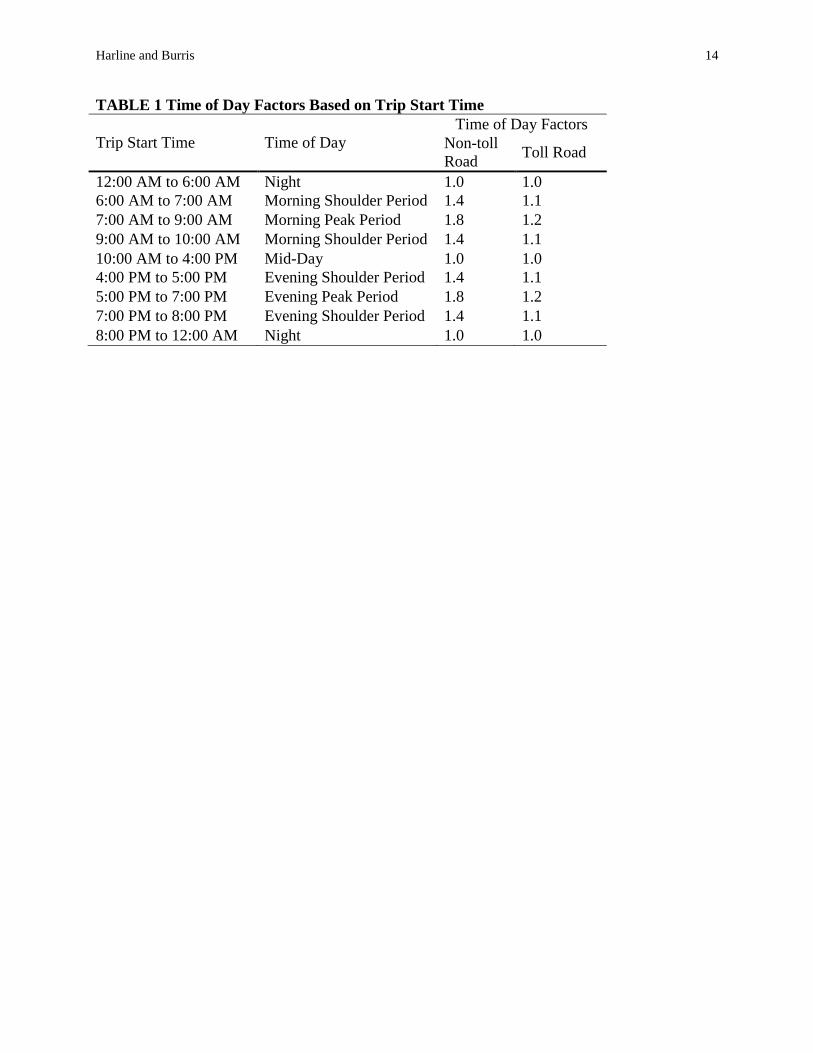
TDF = time of day factor, as noted in Table 1

Once the total trip travel time was determined, travel time variability was determined as a

percentage of travel time as discussed in the following paragraphs. Finally, a toll rate in cents per

mile was assigned to the toll road mode.

SP Trip Attribute Assignment

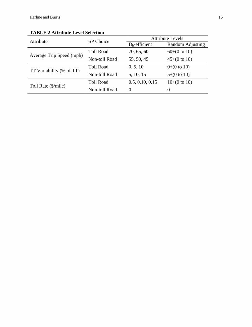
Each route choice in each SP question included a travel time, travel time variability, and toll rate

as determined using one of two SP design methods. The design method to be used was

determined randomly prior to the presentation of the questions to the respondent. Approximately

half of the respondents were presented with SP questions where the attributes of the questions

were determined by a Bayesian D-Efficient (Db-efficient) design, with the other half determined

using a Random Adjusting (RA) design (see Table 2).

The Random Adjusting survey design utilizes respondent feedback over the course of

multiple SP questions by adjusting trip attributes after each question. In this survey, average trip

speed and travel time variability varied randomly within the constraints listed in Table 2. Toll

rate, however, varied with respect to the respondent’s route choice from the previous question.

The original toll rate presented to a respondent was a random rate between 10 and 20 cents per

mile. If a respondent chose the toll road option in the previous question, the toll rate increased by


a random percentage between 30% and 90%. If a respondent chose the non-toll road option, the

toll rate decreased by 35% to 70%. In this way, trip cost increased or decreased contingent on

previous feedback from the respondent in an attempt to arrive at a given respondent's true

willingness to pay. This is similar to the double-bounded contingent valuation approach used by

economists (17,18). The discrete response contingent valuation approach is a special case of a

choice modeling exercise.

The N-Gene software package was used to generate the Db-efficient design for this

survey design strategy. To proceed, a random parameter (or mixed) panel logit (rppanel) was

specified for the discrete choice model, and the priors were simulated using 400 Halton draws

drawn from prior distributions based on previous survey results of freeway travelers in Texas.

Each respondent was randomly given all choice sets from one of the blocks. The Db-error for the

design was found to be 0.71, which indicates an efficient design.

While the SP design usually provided for realistic travel scenarios from which the

respondent can choose, several constraints were placed on the attributes to prevent the travel

scenario from exceeding certain limits. First, travel speed was constrained, such that if Equation

1 yielded an average trip speed that exceeded 85 mph in the case of the toll road option or 75

mph in the case of the non-toll road option, the SP design defaulted to a travel time that would

yield an average trip speed of 85 mph and 75 mph for the respective options. This range of

speeds was selected to best represent SH 130 in Austin, which during the time of the study, had a

speed limit of 85 mph. Second, the maximum travel time as found using Equation 1 that a

respondent was presented was 60 minutes. This constraint was placed to present a more realistic

travel option to the average respondent. Lastly, in the case of respondents presented with the RA

design, the toll rate was limited to a range of 10 to 55 cents per mile. Due to the nature of the

Random Adjusting design, it was possible that the survey could present toll rates that exceeded

this high a rate unless this constraint was provided.

Stated-Preference Question Graphics

As seen in Figure 1, each respondent may have been presented with a set of stated

preference questions that either included a picture representing traffic conditions typical of the

trip characteristics presented, or the stated preference questions did not include such a picture.

Each respondent was randomly assigned the picture or no-picture design before the first SP

question was presented.

Upon calculation of the trip characteristics, a picture was assigned to each option that was

based on the option’s average speed (see Figure 2). If the speed was greater than or equal to 65

mph, the respondent saw a picture of “light” traffic next to the option graphic. If the average

speed was between 50 mph and 60 mph, the survey displayed a picture of “medium” traffic, and

if the average speed was less than or equal to 50 mph, the respondent was presented a picture of

“heavy” traffic. The pictures also varied in setting as we had two different routes available – a

tolled route and an untolled route. The presentation of these pictures provided the basis for study

among these results to determine whether the pictures influenced responses of survey

respondents.

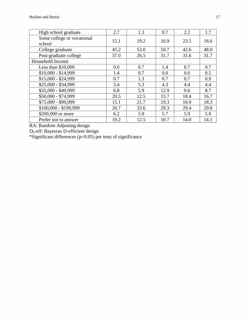
ANALYSIS OF SURVEY RESULTS Contrasting the survey demographics with Austin demographics as provided in the 2011

American Community Survey, it was found that the population with no higher education was

underrepresented in the survey responses. Additionally, nearly 30 percent of survey respondents


described their household income as between $100,000 to $199,999 per year, with over 70

percent of respondents earning more than $50,000 per year. It is evident that the sample

population overrepresented the total population in higher education and training as well as high

income, which may be due to the nature of the advertising of the survey, as the primary

advertising was performed on social networks, public radio, and news websites. It is possible that

the sample could have better represented the whole population through a random selection

process of all TxTag users, or possibly through Department of Motor Vehicle registrations which

may have a greater likelihood of reaching more of the lesser-educated and poor population.

Nonetheless, the driving population typically exhibits characteristics that are different from the

non-driving population, so some differences between survey respondent socio-demographics and

those of the general population are expected.

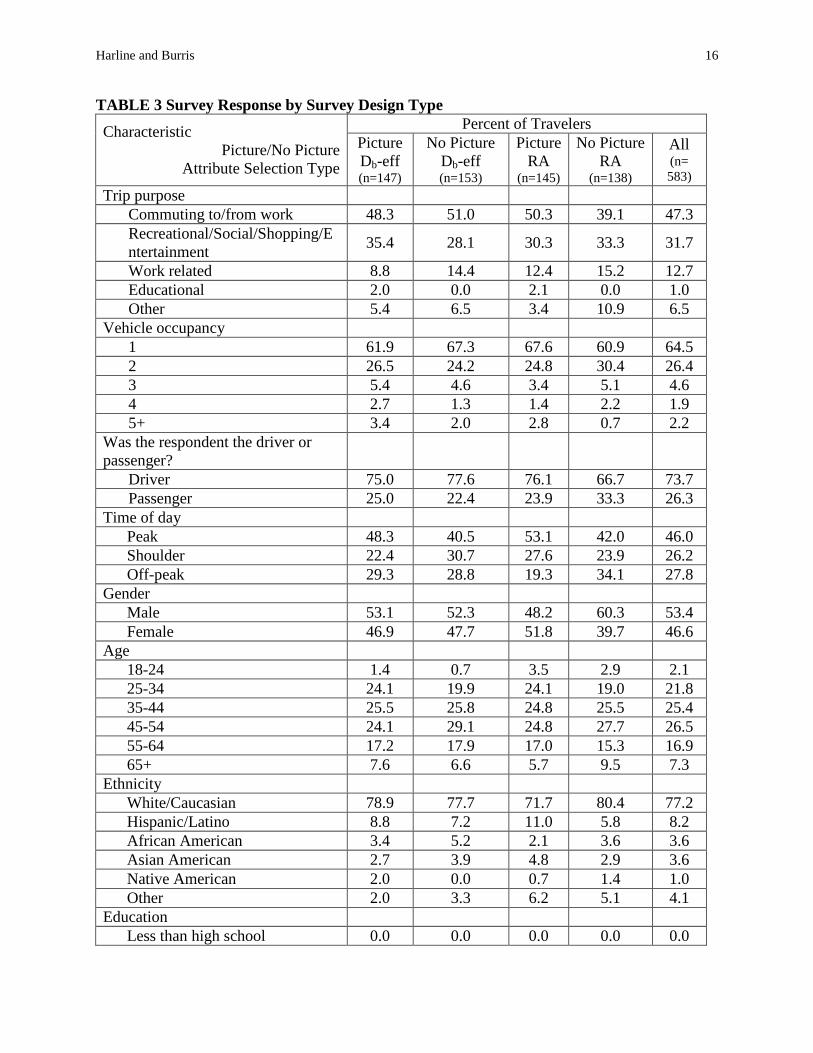
Survey responses were cross-tabulated by the four survey design types check for

consistency across survey designs. To perform a statistical test of significance across survey

design type the chi-squared test was used for those data which were categorical but not ordinal in

nature (i.e. day of the week, or time of the day). Kendall’s Tau-b test was used for ordinal data

(e.g. how many times the respondent used the toll road in the previous week). For continuous

data such as travel time for the respondent’s most recent trip, an Analysis of Variance procedure

was used. From this analysis it was determined that survey respondents exhibited no statistically

significant differences across survey design pools (see Table 3).

Cross-tabulated results of traveler characteristics with respect to stated route choice

provide insight as to which traveler characteristics and preferences may be significant factors in

predicting route choice behavior. First, several key characteristics of a traveler’s most recent trip

on Austin area freeways were shown to be significantly different by respondent’s route choice,

including characteristics such as trip purpose, the day of the week the respondent’s most recent

trip, and the duration of that trip. In the case of trip purpose, respondents who stated that their

most recent trip was for commuting and work-related purposes were more likely to choose a toll

road alternative in the SP section of the survey, while recreational travelers tended to choose the

non-toll alternative. Since the work-related option was described to the respondent as “not

commuting”, but rather trips between one work-related task to another, it is likely that many

respondents who chose this option would not bear the cost of the toll in the hypothetical SP

exercise, and thus may be more inclined to choose the toll road alternative. These findings

helped to develop the route choice models discussed in the following section.

Multinomial Logit Models of Route choice

Several panel-effects mixed MNL models of respondent route choice were developed using the

choice anlaysis software NLOGIT Version 5. Models developed with this software utilized the

mixed (or random parameters) logit technique in order to better understand what variables most

influence route choice. The mixed-logit modeling technique is ideal for this data due to the

presence of respondent heterogeneity in the error terms of the results (14). To account for

respondent heterogeneity in the models, the parameter for travel time (βTT) and the toll road

alternative-specific constant (ASC) parameter (βASC_TR) were randomized using a Halton

sequence, simulating a random selection process to vary the distribution of those parameters

(14). The Halton sequence for these data used a triangular distribution for the toll and toll road

ASC parameters. For these data, it was determined to use a Halton sequence with a total of 500

draws to account for heterogeneity across respondents’ three choice observations, as this number


of draws presented the model with the best goodness-of-fit across a range of possible draws that

were tested (14).

Table 4 provides the coefficients and significance (in parentheses) of each parameter

across all survey design types, as it pertains to the model that exhibited the best goodness-of-fit

and predictive ability measures (see Equation 2 for the resulting utility function). The value of

travel time savings (VTTS) and value of travel time reliability (VTTR) were also calculated from

model parameters. VTTS for any of the models in this setting is equal to (βTT/βTOLL)*60, and

VTTR was calculated by (βTTV/βTOLL)*60. The best model across all survey design types yields a

VTTS of $16.07/hour, with a VTTR of $2.00/hour. A 95% confidence interval for the VOTT

was also derived using the process described by Hensher and Greene (19).

(2)

where: Ui = total utility of alternative i

TT = total travel time (in minutes)

TTV = total travel time variability (in minutes)

Weekday = dummy parameter, 1 indicates trip occurs on a weekday

ASCTR = alternative-specific constant for the toll road alternative

Toll = total trip toll (in dollars)

Time of Day = dummy parameter, 1 indicates trip occurred during a peak hour

Male = dummy parameter, 1 indicates male respondent

High Income = dummy parameter, 1 indicates respondent income >$100,000/yr

Work Related = dummy parameter, 1 indicates a work-related trip purpose

It is evident from the ML model estimation across survey design types that the Db-

efficient attribute selection design with pictures offers the best adjusted ρc2 measure, though the

VTTS estimate of $28.78/hr for that model is much higher than the estimate across the whole

sample ($16.07/hr), as well as in comparison to estimates based on data parsed by survey design

type. The different models generally had similar predictive ability, except the RA with pictures

design had a somewhat lower percent correct prediction rate. Despite these differences, since the

mean VTTS estimate for the whole dataset lies within the 95% confidence interval of each of the

subsets there is no significant evidence that any survey design yields VTTS estimates that are

significantly different from the whole dataset.

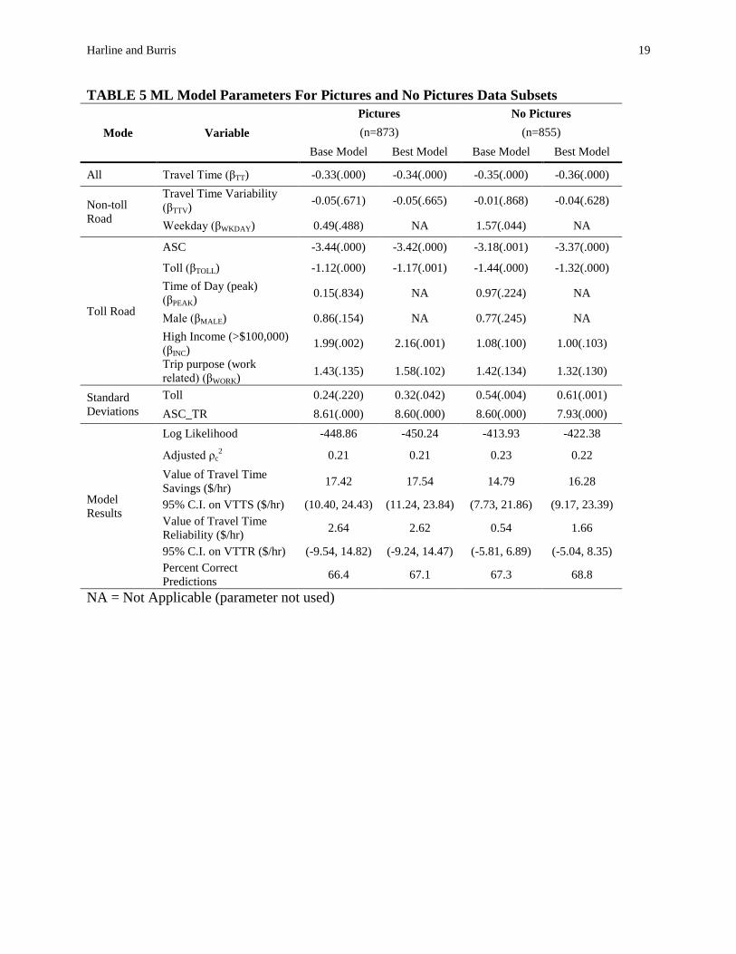
In Table 5, model results for the design types with and without pictures are summarized.

For this specific subset of data, an effort was made to discover the best fitting model. Therefore,

Table 5 shows the results from both the base model and another model that was optimized for the

Pictures and No Pictures design datasets. From these models it is easier to see the impact that the

presence of traffic images had on SP choice behavior.

First, model results show similar performance across both datasets with respect to

predictive ability and the adjusted ρ2. When comparing VTTS, the Picture dataset estimated a

value of $1.26/hr higher than the No Picture dataset. This result is consistent with previous

findings that presenting traffic images as a supplement to trip attributes in the SP setting will

yield a higher VTTS due to the presence of a congestion premium. However, closer examination


of the 95% confidence interval reveals that the difference is within the bounds of the sampling

error. These results regarding the VTTS calculation failed to find any significant evidence that

pictures of traffic characteristics induced a significant influence on route choice in this survey.

Likewise, while the VTTR estimate is lower for the No Picture datasetbut not statistically

different at a 95% level of confidence. The VTTS, VTTR, percent correct and Adjusted ρc2 from

the best picture and no-picture models were surprisingly similar.

CONCLUSIONS With traveler options becoming more complex, as in the case of express lanes or managed lanes,

it may be necessary to enhance surveys with pictures to help travelers answer survey questions.

In this research, a stated-preference survey was developed to measure the influence of traffic

images on route choice. The Austin Travel Survey also collected information about the most

recent trip of each respondent, which was then pivoted to develop base trip characteristics for the

SP portion of the survey. Trip attributes were then randomly assigned to each respondent using

either a Db-efficient or Random Adjusting design. Then, half of the respondents would be shown

an image of traffic in their SP questions alongside of a lexicographic description of trip

attributes.

Survey responses were then cross-tabulated to test for significant differences between

survey design type subsets. There were no significant differences between responses for each

survey design type. A panel effects mixed MNL model was built to estimate the respondent's

choice behavior. Overall model parameters discovered no evidence to support the assertion that

traffic image presentation had a significant effect on route choice.

While this study was able to present images that roughly corresponded to trip

characteristics (via the average trip speed attribute), this research was limited in its ability to

study the effect of image presentation in the context of a pictorial format with minimal text. Due

to the format of the SP questions, it is possible that a respondent viewed the traffic images as

being a supplemental piece of information, secondary to the lexicographic description of trip

attributes. Therefore, it is possible that respondents did not base their decisions on the traffic

image, since trip attributes were summarized in the text. In future studies, a greater disparity

could be introduced in how heavily a respondent must rely on traffic pictures to understand trip

characteristics of the route choice. But based on the results of this survey, pictures are not worth

1000 words in a SP question related to toll road use. However, with traveler decisions becoming

more complex, we feel that more research into pictorial aids for choices in SP surveys is

warranted.

REFERENCES

(1) Mazzotta, M.J., Opaluch, J.J. Decision making when choices are complex: a test of

Heiner’s hypothesis. Land Economics, Vol. 71, 1995, pp. 500-515.

(2) Wang, D., Jiuqun, L., Timmermans, H.J.P. Reducing respondent burden, information

processing effort and incomprehensibility in stated preference surveys: principles and

properties of paired conjoint analysis. In Transportation Research Record: Journal of the

Transportation Research Board, No. 1768, Transportation Research Board of the National

Academies, Washington, D.C., 2001, pp. 71-78.

(3) Rose, J.M., Bliemer, M., Hensher, D.A., Collins, A.T. Designing efficient stated choice

experiments in the presence of reference alternatives. Transportation Research Part B, Vol.

42, 2008, pp. 395-406.


(4) Rizzi, L., Limonado, J.P., Steimetz, S.S.C. The impact of traffic images on travel time

valuation in stated-preference choice experiments. Transportmetrica, Vol. 8, No. 6, 2012,

pp. 427-442.

(5) Small, K. A., Noland, R., Chu, X. Valuation of Travel-Time Savings and Predictability in

Congested Conditions for Highway User-Cost Estimation. National Cooperative Highway

Research Program, Report 431, 1999.

(6) Arentze, T., Borgers, A., Timmermans, H., DelMistro, R. 2003. Transport stated choice

responses: effects of task complexity, presentation format and literacy. Transportation

Research Part E, Vol. 39, pp. 229-244.

(7) Heiner, R.A. 1983. The Origin of Predictable Behavior. American Economic Review, Vol.

73, pp. 560-595.

(8) McFadden, D. 1974. The Measurement of Urban Travel Demand. Journal of Public

Economics, Vol. 3, pp. 303-328.

(9) Hess, S., Rose, J.M., Polak, J. 2010. Non-trading, Lexicographic and Inconsistent Behavior

in Stated Choice Data. Transportation Research Part D, Vol. 15, pp. 405-417.

(10) Caussade, S., Ortuzar, J., Rizzi, L., and Hensher, D. 2005. Assessing the influence of

design dimensions on stated choice experiment estimates. Transportation Research Part A,

Vol. 39, pp. 621-640.

(11) Stopher, P.R., Hensher, D.A. Are more profiles better than less? Searching for parsimony

and relevance in stated choice experiments. Presented at the 79th

Annual Meeting of the

Transportation Research Board, Washington, D.C., 2000.

(12) Hensher, D.A. 2006. How do respondents handle stated choice experiments? Attribute

procession strategies under varying information load. Journal of Applied Econometrics,

Vol. 21, pp. 861-878.

(13) Hess, S., Hensher, D. A., Daly, A. 2012. Not Bored Yet - Revisiting Respondent Fatigue in

Stated Choice Experiments. Transportation Research Part A, Vol. 46, pp. 626-644.

(14) Hensher, D.A., Rose, J.M., Greene, W.H. Applied Choice Analysis: A Primer. Cambridge

University Press, 2005.

(15) Walker, Joan L. and Ben-Akiva, Moshe. Advances in Discrete Choice: Mixture Models. A

Handbook of Transport Economics, 2011, p. 160.

(16) National Household Travel Survey, 2009, http://nhts.ornl.gov/download.shtml.

(17) Hanemann, W.M., Loomis, J., Kanninen, B. 1991. Statistical Efficiency of Doublebounded

Dichotomous Choice Contingent Valuation. American Journal of Agricultural Economics,

Vol. 73, pp. 1255-1263.

(18) Kanninen, B.J., 1993. Optimal Experimental Design for Double-Bounded Dichotomous

Choice Contingent Valuation. Land Economics, Vol. 69, Issue 2, pp. 138-146.

(19) Hensher, D.A., Greene, W.H. The Mixed-Logit Model: The State of Practice. ITS Working

Paper, ITS-WP-02-01, Institute of Transport Studies (Sydney & Monash), 2002.


List of Tables

TABLE 1 Time of Day Factors Based on Trip Start Time

TABLE 2 Attribute Level Selection

TABLE 3 Survey Response by Survey Design Type

TABLE 4 ML Model Parameters Across Survey Design Types

TABLE 5 ML Model Parameters For Pictures and No Pictures Data Subsets

List of Figures

FIGURE 1 Example SP question including supplemental traffic images.

FIGURE 2. Survey image representing light, medium, and heavy traffic.


TABLE 1 Time of Day Factors Based on Trip Start Time

Trip Start Time Time of Day

Time of Day Factors

Non-toll

Road Toll Road

12:00 AM to 6:00 AM Night 1.0 1.0

6:00 AM to 7:00 AM Morning Shoulder Period 1.4 1.1

7:00 AM to 9:00 AM Morning Peak Period 1.8 1.2

9:00 AM to 10:00 AM Morning Shoulder Period 1.4 1.1

10:00 AM to 4:00 PM Mid-Day 1.0 1.0

4:00 PM to 5:00 PM Evening Shoulder Period 1.4 1.1

5:00 PM to 7:00 PM Evening Peak Period 1.8 1.2

7:00 PM to 8:00 PM Evening Shoulder Period 1.4 1.1

8:00 PM to 12:00 AM Night 1.0 1.0


TABLE 2 Attribute Level Selection

Attribute SP Choice Attribute Levels

Db-efficient Random Adjusting

Average Trip Speed (mph) Toll Road 70, 65, 60 60+(0 to 10)

Non-toll Road 55, 50, 45 45+(0 to 10)

TT Variability (% of TT) Toll Road 0, 5, 10 0+(0 to 10)

Non-toll Road 5, 10, 15 5+(0 to 10)

Toll Rate ($/mile) Toll Road 0.5, 0.10, 0.15 10+(0 to 10)

Non-toll Road 0 0


TABLE 3 Survey Response by Survey Design Type

Characteristic

Picture/No Picture

Attribute Selection Type

Percent of Travelers

Picture

Db-eff (n=147)

No Picture

Db-eff (n=153)

Picture

RA (n=145)

No Picture

RA (n=138)

All (n=

583)

Trip purpose

Commuting to/from work 48.3 51.0 50.3 39.1 47.3

Recreational/Social/Shopping/E

ntertainment 35.4 28.1 30.3 33.3 31.7

Work related 8.8 14.4 12.4 15.2 12.7

Educational 2.0 0.0 2.1 0.0 1.0

Other 5.4 6.5 3.4 10.9 6.5

Vehicle occupancy

1 61.9 67.3 67.6 60.9 64.5

2 26.5 24.2 24.8 30.4 26.4

3 5.4 4.6 3.4 5.1 4.6

4 2.7 1.3 1.4 2.2 1.9

5+ 3.4 2.0 2.8 0.7 2.2

Was the respondent the driver or

passenger?

Driver 75.0 77.6 76.1 66.7 73.7

Passenger 25.0 22.4 23.9 33.3 26.3

Time of day

Peak 48.3 40.5 53.1 42.0 46.0

Shoulder 22.4 30.7 27.6 23.9 26.2

Off-peak 29.3 28.8 19.3 34.1 27.8

Gender

Male 53.1 52.3 48.2 60.3 53.4

Female 46.9 47.7 51.8 39.7 46.6

Age

18-24 1.4 0.7 3.5 2.9 2.1

25-34 24.1 19.9 24.1 19.0 21.8

35-44 25.5 25.8 24.8 25.5 25.4

45-54 24.1 29.1 24.8 27.7 26.5

55-64 17.2 17.9 17.0 15.3 16.9

65+ 7.6 6.6 5.7 9.5 7.3

Ethnicity

White/Caucasian 78.9 77.7 71.7 80.4 77.2

Hispanic/Latino 8.8 7.2 11.0 5.8 8.2

African American 3.4 5.2 2.1 3.6 3.6

Asian American 2.7 3.9 4.8 2.9 3.6

Native American 2.0 0.0 0.7 1.4 1.0

Other 2.0 3.3 6.2 5.1 4.1

Education

Less than high school 0.0 0.0 0.0 0.0 0.0


High school graduate 2.7 1.3 0.7 2.2 1.7

Some college or vocational

school 15.1 19.2 16.9 23.5 18.6

College graduate 45.2 53.0 50.7 42.6 48.0

Post-graduate college 37.0 26.5 31.7 31.6 31.7

Household Income

Less than $10,000 0.0 0.7 1.4 0.7 0.7

$10,000 - $14,999 1.4 0.7 0.0 0.0 0.5

$15,000 - $24,999 0.7 1.3 0.7 0.7 0.9

$25,000 - $34,999 3.4 5.3 4.3 4.4 4.4

$35,000 - $49,999 6.8 5.9 12.9 9.6 8.7

$50,000 - $74,999 20.5 12.5 15.7 18.4 16.7

$75,000 - $99,999 15.1 21.7 19.3 16.9 18.3

$100,000 - $199,999 26.7 33.6 29.3 29.4 29.8

$200,000 or more 6.2 5.9 5.7 5.9 5.9

Prefer not to answer 19.2 12.5 10.7 14.0 14.1

RA: Random Adjusting design

Db-eff: Bayesian D-efficient design

*Significant differences (p<0.05) per tests of significance


TABLE 4 ML Model Parameters Across Survey Design Types

Mode Variable

All Survey

Design Types

Db-efficient

with Picture

Db-efficient

without

Picture

RA with

Picture

RA without

Picture

(n=1728) (n=438) (n=447) (n=435) (n=408)

All Travel Time (βTT) -0.33(.000) -0.42(.000) -0.48(.000) -0.38(.006) -0.22(.108)

Non-toll

Road

Travel Time Variability

(βTTV) -0.04(.506) 0.05(.846) 0.15(.162) -0.19(.286) -0.12(.407)

Weekday (βWKDAY) 0.90(.064) 0.98(.295) 0.31(.759) 0.48(.758) 2.38(.072)

Toll Road

ASC -3.44(.000) -4.85(.000) -3.10(.012) -1.26(.471) -3.35(.052)

Toll (βTOLL) -1.22(.000) -0.88(.004) -1.76(.000) -2.00(.003) -1.28(.002)

Time of Day (peak)

(βPEAK) 0.62(.233) 1.19(.252) 0.09(.929) -1.93(.217) 1.62(.213)

Male (βMALE) 0.81(.050) 0.72(.358) -0.12(.893) 1.45(.290) 1.60(.172)

High Income

(>$100,000) (βINC) 1.46(.001) 2.46(.006) 1.31(.113) 1.85(.194) 1.09(.303)

Trip purpose (work

related) (βWORK) 1.32(.043) 1.78(.171) 1.60(.110) 1.25(.513) 0.85(.622)

Standard

Deviations

Travel Time 0.31(.011) 0.45(.025) 0.87(.000) 0.48(.208) 0.23(.655)

ASC_TR 8.79(.000) 6.94(.000) 5.54(.004) 13.11(.001) 10.50(.002)

Model

Results

Log Likelihood -866.32 -199.05 -207.77 -241.37 -198.77

Adjusted ρc2 0.23 0.29 0.27 0.11 0.14

Value of Travel Time

Savings ($/hr) 16.07 28.78 16.53 11.37 10.12

95% C.I. on VTTS ($/hr) (11.25, 20.88) (14.89, 42.66) (7.99, 25.08) (3.35, 19.40) (-2.23, 22.48)


Reliability ($/hr) 2.00 -3.47 -5.04 5.62 5.69

95% C.I. on VTTR ($/hr) (-3.90, 7.91) (-38.39, 31.46) (-12.10, 2.02) (-4.71, 15.94) (-7.76, 19.14)

Percent Correct

Predictions 68.0 70.8 69.6 62.1 72.5


TABLE 5 ML Model Parameters For Pictures and No Pictures Data Subsets

Mode Variable

Pictures No Pictures

(n=873) (n=855)

Base Model Best Model Base Model Best Model

All Travel Time (βTT) -0.33(.000) -0.34(.000) -0.35(.000) -0.36(.000)

Non-toll

Road

Travel Time Variability

(βTTV) -0.05(.671) -0.05(.665) -0.01(.868) -0.04(.628)

Weekday (βWKDAY) 0.49(.488) NA 1.57(.044) NA

Toll Road

ASC -3.44(.000) -3.42(.000) -3.18(.001) -3.37(.000)

Toll (βTOLL) -1.12(.000) -1.17(.001) -1.44(.000) -1.32(.000)

Time of Day (peak)

(βPEAK) 0.15(.834) NA 0.97(.224) NA

Male (βMALE) 0.86(.154) NA 0.77(.245) NA

High Income (>$100,000)

(βINC) 1.99(.002) 2.16(.001) 1.08(.100) 1.00(.103)

Trip purpose (work

related) (βWORK) 1.43(.135) 1.58(.102) 1.42(.134) 1.32(.130)

Standard

Deviations

Toll 0.24(.220) 0.32(.042) 0.54(.004) 0.61(.001)

ASC_TR 8.61(.000) 8.60(.000) 8.60(.000) 7.93(.000)

Model

Results

Log Likelihood -448.86 -450.24 -413.93 -422.38

Adjusted ρc2 0.21 0.21 0.23 0.22


Savings ($/hr) 17.42 17.54 14.79 16.28

95% C.I. on VTTS ($/hr) (10.40, 24.43) (11.24, 23.84) (7.73, 21.86) (9.17, 23.39)


Reliability ($/hr) 2.64 2.62 0.54 1.66

95% C.I. on VTTR ($/hr) (-9.54, 14.82) (-9.24, 14.47) (-5.81, 6.89) (-5.04, 8.35)

Percent Correct

Predictions 66.4 67.1 67.3 68.8

NA = Not Applicable (parameter not used)


FIGURE 1 Example SP question including supplemental traffic images.


FIGURE 2 Survey image representing light, medium, and heavy traffic.

the impact of traffic images on route choice and …ceprofs.tamu.edu/mburris/papers/impact of...

Documents