The Impact of Skilled Foreign Workers on Firms:

an Investigation of Publicly Traded U.S. Firms ∗

Anirban GhoshGeorgetown University

Anna Maria MaydaGeorgetown University and CEPR

Francesc OrtegaQueens College, CUNY

January 19, 2016

Abstract

Many U.S. businessmen are vocally in favor of an increase in the number of H-1B visas.Is there systematic evidence that this would positively affect firms’ productivity, sales,employment or profits? To address these questions we assemble a unique dataset thatmatches all labor condition applications (LCAs) – the first step towards H-1B visasfor skilled foreign-born workers in the U.S. – with firm-level data on publicly tradedU.S. firms (from Compustat). Our identification is based on the sharp reduction in theannual H-1B cap that took place in 2004, combined with information on the degreeof dependency on H-1B visas at the firm level as in Kerr and Lincoln (2010). Themain result of this paper is that if the cap on H-1B visas were relaxed, a subset offirms would experience gains in average labor productivity, firm size, and profits. Theseare firms that conduct R&D and are heavy users of H-1B workers – they belong tothe top quintile among filers of LCAs. These empirical findings are consistent with aheterogeneous-firms model where innovation enhances productivity and is subject tofixed costs.

Keywords: Immigration, H1-B Visas, Firms, Innovation

∗We thank Thomas Chaney, Benjamin Elsner, Corrado Giulietti, William Kerr, Chad Sparber, Thijsvan Rens, Aysegul Sahin, and seminar participants in Bologna, Cornell, ERWIT-CEPR, IZA, Queens Col-lege, Syracuse, the SNF Sinergia - CEPR conference on Economic Inequality, Labor Markets and Interna-tional Trade, and the 2016 LERA session at the ASSA for helpful comments. The authors thank NOR-FACE/TEMPO and the Institute for the Study of International Migration (ISIM) at Georgetown Universityfor financial support. Corresponding authors: Francesc Ortega (fortega@qc.cuny.edu), and Anna MariaMayda (amm223@georgetown.edu).

“I want to emphasize that to address the shortage of scientists and engineers, we

must do both – reform our education system and our immigration policies. If we

don’t, American companies simply will not have the talent they need to inno-

vate and compete.”(Bill Gates, Testimony at the U.S. House of Representatives,

Committee on Science and Technology on March 12, 2008)

1 Introduction

As our opening quote illustrates, CEOs of large U.S. corporations often advocate passion-

ately in favor of an increase in the number of H-1B visas. They argue that there is a shortage

of skilled workers in the U.S. labor market in some fields and that, unless the cap on H-1B

visas is raised, their firms will not be able to grow, and their innovation efforts and R&D

activities may be at risk.1 The goal of this paper is to evaluate the effects of H-1B visas on

firms’ productivity, sales, employment and profits.

There is abundant anecdotal evidence that the contribution of immigrants to innovation,

entrepreneurship and education is substantial in the U.S.. Immigrants account for about one

quarter of U.S.-based Nobel Prize recipients between 1990 and 2000, of founders of public-

venture-backed U.S. companies in 1990-2005, and of founders of new high-tech companies

with at least one million dollars in sales in 2006 (Wadhwa et al. (2007)). These authors also

report that 24 percent of all patents originating from the U.S. are authored by non-citizens.2

In addition several studies have established a connection between skilled immigration

and patenting activity (Hunt and Gauthier-Loiselle (2010), Kerr and Lincoln (2010) and

Parrotta et al. (2014b)), although a recent study by Doran et al. (2014) questions this

finding and has re-opened the debate. Thus even if we assume that skilled immigration

increases the number of patents, it is not known whether the resulting patents translate

into innovation with direct effects on firm performance.3 By focusing on relevant outcomes,

1Several large American technology companies, such as Microsoft, Amazon or Facebook, have recentlyestablished offices in Vancouver (Canada). One of the main reasons seems to be the difficulty in obtaining H-1B visas for new hires in the United States and the larger abundance of (foreign) skilled labor in Vancouver.Karen Jones, Microsoft’s deputy general counsel, put it in the following words: “The U.S. laws clearly didnot meet our needs. So we have to look to other places.” (Bloomberg Businessweek 2014).

2In addition Borjas (2005) shows that foreign students receive over fifty percent of all doctorates grantedin the field of engineering. As a share of college-educated employment, the foreign-born population in theUnited States has increased from 7 percent in 1980 to over 15 percent in 2010 (Peri et al. (2013)). Incomparison the foreign-born share in overall employment increased from 6.4 to 16 percent over the sameperiod. The original data source is the U.S. Census, population ages 18 to 65.

3Since the early 1990s there has been an explosion in the number of patents. As argued by Hall andZiedonis (2001), in some industries (e.g. semiconductors) the increase in patenting may be due to strategicuse by firms. Namely, obtaining patents may allow firms to exercise hold-up or prevent competitors from

1

such as sales, productivity, employment, and profits, we can examine whether the positive

effect of skilled immigration on patenting activity documented in the literature in fact

translates into improved firm performance. Our results suggest that this is indeed the case.

Thus, H-1B workers appear to increase innovation and improve firm performance.

The main goal of our paper is to evaluate the claim that the current quota on H-1B visas

is hampering the innovation and growth of U.S. firms, and to examine whether all firms

benefit from these visas or only a subset of them. To do so we assemble a unique dataset

that matches the universe of labor condition applications (LCAs) – the first step towards H-

1B visas for skilled foreign-born workers in the U.S. – with firm-level data from Compustat,

which includes all publicly traded U.S. firms. The merged data set allows us to estimate,

at the firm level, the impact of skilled migration on the sales, productivity, employment,

profits, and R&D expenditure of publicly traded U.S. firms. We do so employing flexible

specifications that allow for non-linear effects.

Our identification is based on a sharp change in policy, namely the 2004 reduction in the

annual H-1B cap – which offers an opportunity to identify the causal effect of H-1B workers

on firm outcomes.4 Since we do not observe the actual number of H-1B workers in the firm

and, even if we did, this variable would be clearly endogenous, we estimate a difference-in-

difference specification where the impact of the treatment (the exogenous change in policy)

is compared across different categories of firms. Specifically, we follow Kerr and Lincoln

(2010) and use the number of LCAs in 2001 to measure each firm’s degree of dependency on

H-1B visas. We compare the change in outcomes before and after the policy change across

firms, within the same industry, that are more dependent on H-1B visas (the “treatment

group”) and less dependent firms (“the control group”).5 Since the overall H-1B cap was

sharply reduced between the two years, we expect firms that were initially more dependent

on H-1B visas to display worse outcomes, namely, lower growth in productivity, firm size

(employment and sales), and profits.

We have two main results. First, we find that increases in the number of H-1B workers

lead to growth in productivity, firm size, and profits. However, not all firms benefit equally

from an increase in the cap on H-1B visas. According to our estimates, the relationship

between H-1B workers and measured firm outcomes is highly non-linear. Only firms that file

doing so. A very interesting account of the abuse of patents by some firms (patent trolls) is examined in a2011 episode of ‘This American Life’ (episode 441: When Patents Attack!).

4Between 2001 and 2003 the annual cap on H-1B visas was 195,000. In year 2004 it was reduced to 65,000visas. The cap was raised again to 85,000 visas in 2006.

5The paper by Mitaritonna et al. (2014) rationalizes why some firms use immigrant workers while othersdo not and the consequences of supply shocks at the regional level on firm-level productivity.

2

a relatively large number of applications for H-1B visas appear to benefit from increases in

the cap and, conversely, are more negatively affected when this cap is reduced. Secondly, we

find that the effects are driven by firms that consistently conduct R&D activity, in addition

to relying on H-1B workers.

Our empirical findings can be rationalized with a simple monopolistic competition model

where firms are heterogeneous in initial productivity. These firms can choose to set up a

lab to conduct R&D, which requires hiring skilled workers. To be viable, a lab requires a

minimum size, in terms of the number of skilled workers, which amounts to a fixed cost.

In addition there is a shortage skilled native workers and some firms need to rely on H-1B

visas. Firms that are successful in setting up a lab experience an improvement in their

productivity, which in turn has positive effects on sales, employment and profits. One of

the strengths of our paper is that we are able to provide evidence for positive effects of H-1B

workers on all these firm-level outcomes. In contrast, most of the literature has focused on

one of these outcomes at a time, often relying on less comprehensive data.

Our paper is related to the large body of literature trying to measure the effects of

different dimensions of globalization, such as trade and immigration, on firms, with an

emphasis on implications for productivity and innovation. We discuss each of these in

turn. We begin by briefly reviewing the relevant literature on (skilled) immigration and

innovation. A seminal study in this literature is Kerr and Lincoln (2010) who focus on

the effects of H-1B visas on patenting activity. While closely related, our analysis departs

from theirs in important ways. First, our dataset contains the universe of publicly traded

firms in the U.S. After merging it with the data on labor-condition applications (LCAs),

we end up with almost four thousand firms. In contrast, the firm-level analysis in Kerr

and Lincoln (2010) is based on a much smaller sample size (of only 77 firms).6 Second, we

broaden the scope of the analysis by examining a broader set of outcomes, which includes

firm productivity, sales, profits, R&D expenditures, and TFP. Third, as noted above, in

terms of identification, we rely on the time-variation arising from a single policy event, the

large reduction in the national cap for H-1B visas that took place in year 2004 (Figure 1).

In contrast Kerr and Lincoln exploit year-to-year variation in the stock of H-1B visas.7 Our

6Moreover these firms have been selected on the basis of high patenting activity, their outcome of interest,or of heavy use of labor condition applications. In contrast in our data the majority of firms did not file anyLCAs, although heavy users are also part of our dataset. Thus our median firm is very different from theirs,and representative of all public firms in the U.S.

7We decided not to rely on year-to-year variation in the national cap (or stock of H-1B visas). Because ofimplementation delays, deferrals, or reporting inaccuracies, the data are fairly noisy at an annual frequency.In addition computing the stock of visa holders requires a number of assumptions and imputations (Lowell(2000)), introducing further noise.

3

paper is also related to the forthcoming paper by Pekkala-Kerr et al. (n.d.), which uses

the same empirical strategy as Kerr and Lincoln (2010) to analyze the impact of hiring

young skilled immigrants on the hiring and employment of several groups of skilled native

workers. This paper uses administrative microdata from the U.S. Census Bureau, which is

extremely accurate. However, as in Kerr and Lincoln (2010), the focus is on a subset of

firms – specifically an unbalanced panel of 319 firms, selected on the basis of employment

and patenting activity.

Our paper is also related to the work of Hunt and Gauthier-Loiselle (2010). Exploiting

cross-state variation for the United States, these authors find that a one percentage-point

increase in the share of immigrant college graduates in the population leads to an increase

in patents per capita of 9 to 18 percent, and the main reason is that they disproportionately

hold STEM (Science, Technology, Engineering and Mathematics) degrees. Parrotta et al.

(2014b) analyze the connection between worker diversity within a firm and its patenting

activity using data for Denmark. Their results suggest that ethnic diversity leads to more

patenting. Along similar lines, Chellaraj et al. (2008) document that the presence of foreign

graduate students has a positive impact on future patents. More similar to our paper, Peri

et al. (2013) use variation in the H-1B cap to try to identify the effects of increases in

the population of STEM workers in a city on the wages of skilled and unskilled workers in

the same city. They find that H-1B-driven increases in STEM workers are associated with

increases in the wages paid to skilled workers (both in STEM and non-STEM occupations),

and find no evidence of effects on the wages of unskilled workers. An important recent

contribution to this literature is the work by Doran et al. (2014). These authors link data

on H1-B visas, overall employment based on tax records, and patents at the firm level.

Exploiting the visa lottery that took place in fiscal years 2006 and 2007, they analyze the

effects of H-1B visas on patenting and overall firm employment. They find no evidence of

an effect on patenting and at most a moderate effect on overall employment in the firm.

These authors point out that their results are silent regarding the effects of H-1B visas on

firms’ productivity and profits, which we are able to address in our analysis. In addition

Doran et al. (2014) focus their analysis on the median firm, which is relatively small, while

our results suggest that because of the presence of fixed-costs of innovation only large firms

may benefit from H-1B visas.

Let us now turn to the literature on economic openness and productivity. Many studies

have explored the effects of international trade on productivity (see, for example, Melitz

(2003), Pavcnik (2002), Bernard et al. (2007), Melitz and Ottaviano (2008) or Lileeva and

4

Trefler (2010) and Bustos (2011)), which is closely related to our theoretical framework

and our empirical strategy. Our paper is also related to the small literature that studies

the effects of immigration on productivity. However, many of the migration studies rely

on aggregate data and, as a result, require strong identification assumptions and are more

vulnerable to omitted-variable bias.8 These studies typically correlate the immigrant share

in a country or region (a U.S. state or metropolitan statistical area) with aggregate pro-

ductivity levels (as in Quispe-Agnoli and Zavodny (2002), Peri (2012), and Ortega and

Peri (2014)). Several of these studies find that foreign workers have a positive effect on

productivity.9 However, these studies typically are not able to disentangle which part of

the effect arises from spillovers, which requires different identification strategies (Moretti

(2004), Greenstone et al. (2010)).

Very few papers have empirically analyzed the effects of immigration on firm-level pro-

ductivity.10 Paserman (2013) exploits cross-firm and cross-industry variation in the con-

centration of skilled immigrants and finds evidence of a negative correlation between the

immigrant share and output per worker in low-tech industries, whereas the relationship

becomes positive for high-tech industries. Parrotta et al. (2014a) analyze the effects of

diversity within firms on total factor productivity, using a rich matched employeremployee

dataset for Denmark. Their estimates point toward a negative association between ethnic

diversity and firm-level productivity. In ongoing work, Trax et al. (2013) use German estab-

lishment data to estimate the effect of cultural diversity on total factor productivity. Their

results suggest that higher immigrant concentration in a firm does not lead to higher TFP.

However, they find that higher ethnic diversity in the firm or in the region where the firm

is located do appear to have positive effects on TFP at the firm level, consistent with the

findings in Ortega and Peri (2014). Thus the sign and magnitude of the effects of skilled

immigration on firm-level productivity is still an open question.

The rest of the paper is organized as follows. Section 2 presents a theoretical frame-

work that guides the empirical analysis. Section 3 presents the data sources and describes

the matching algorithm. Section 4 presents summary statistics. Section 5 discusses our

8For an overview of the findings in the literature on the economic effects of skilled immigration see, forexample, Bertoli et al. (2012).

9Many studies only use a general measure of immigration. One exception is Ortega and Peri (2014) whodistinguish between the effect of overall immigration and the effect of the diversity of immigrants by countryof birth.

10Teruel-Carrizosa and Segarra-Blasco (2008) explore the effects of immigration on firm profits using datafor Spain. While their dependent variable is profitability at the firm level, they only measure immigrantdensity at the city level. Thus identification is still based on cross-city variation. Dustmann and Glitz (2011)also analyze the effects of immigration into a region on the distribution of firms in that region.

5

empirical strategy. Section 6 presents our main estimates and Section 7 presents extensive

sensitivity analysis. Section 8 discusses the theoretical implications of our empirical findings

and Section 9 concludes.

2 Theoretical framework

Consider a standard monopolistic competition setup where producers vary in their level of

productivity (Jovanovic (1982), Hopenhayn (1992), or Melitz (2003), among many others)

and production is subject to fixed and variable costs. The goal of the model is to derive

predictions for the effects of adding skilled workers on all relevant firm outcomes. For now

we shall assume that skilled workers and, in particular, foreign skilled workers hired through

H-1B visas lead to higher firm productivity and derive a number of implications. Later on

we shall provide empirical evidence based on our data supporting the connection between

skilled labor and firm productivity.

2.1 The economy

Consider a standard monopolistic competition setup where producers differ in their level of

productivity. Specifically, we assume there is a representative consumer with CES prefer-

ences. The utility maximization problem is given by

max

[∫Jy (k)

σ−1σ dk

] σσ−1

s.t.∫Jp (k) y (k) dk = X,

where J is the set of goods available for consumption, X is income, and σ is the elasticity

of substitution. As is well known, the solution to this problem gives rise to the familiar

demand functions where the spending share on each good k is a function of its relative price:

p(k)y(k) =

(p(k)

P

)1−σX, (1)

where P is the price level in the country:

P =

[∫Jp(k)1−σdk

] 11−σ

. (2)

Let us now turn to profit maximization. Each firm wishing to produce is required to pay

a fixed cost f (units of labor). There is one factor of production (“labor”) that firms hire

6

at wage w. Since each firm produces its own unique variety, it faces a downward-sloping

demand curve. In addition, by definition, in the monopolistic-competition model, each

producer is sufficiently small that it takes P as given. As is well known, profit maximization

implies that the price is a constant markup over the marginal cost, given by a(k)w, which

differs across producers.

The profit maximization problem is as follows. The firm with marginal cost a(k) solves:

max[p(k)y(k)− a(k)wy(k)− fwI{y(k)>0}

], (3)

where demand for its variety is given by:

y(k) =

(p(k)

P

)1−σ X

p(k). (4)

2.2 Key predictions

It is straightforward to show that, provided profits are non-negative, the optimal price,

quantity, sales, employment and profits,11 are given by

p[a] =σ

σ − 1aw = maw (5)

y[a] =X

P 1−σ (maw)−σ (6)

py[a] =X

P 1−σ (maw)1−σ (7)

`[a] =X

P 1−σ (mw)−σ a1−σ (8)

π[a] =1

σ

X

P 1−σ (mw)1−σ a1−σ − fw. (9)

Thus, more productive firms (low a) charge lower prices, produce more, have higher

sales, hire more workers, and obtain higher profits. We also note that a firm can always

choose zero output, which delivers zero profits. Thus low productivity (high-a) firms will

not operate. Given X, P and w, the productivity threshold is

π(a) = 0. (10)

To close the model it is customary to impose a free entry condition.12 Furthermore, if we

assume that productivity 1/a is distributed Pareto, then we can solve for the productivity

threshold, the price level, and other equilibrium values analytically. However, we are solely

interested in the following comparative static exercise.

11To lighten notation we drop the k subindex.12In the formulation of Melitz (2003), there is an ex-ante stage where potential firms pay a fixed fee, also

denominated in units of labor, in order to have the right to obtain a productivity draw. Entry into thelottery occurs up to the point where expected profits are driven to zero.

7

2.3 Comparative static: exogenous increase in productivity

Suppose that a firm’s productivity 1/a increased. How would this affect the firm’s size

(in terms of sales and employment) and profits, assuming no change in aggregate variables

(X,P,w)? By virtue of equations (6) - (9), we have that

∆ ln py[a] = (σ − 1)∆ ln a−1 (11)

∆ ln `[a] = (σ − 1)∆ ln a−1 (12)

∆ lnπ[a] =σ − 1

σ∆ ln a−1. (13)

Thus, provided that σ > 1, which is the relevant range for this parameter, an increase

in firm productivity, whatever its source, will lead to increases in firm’s sales (along with

employment and output) and profits. These expressions will be the basis for our empirical

specifications.

2.4 Endogenous productivity

All the previous predictions follow regardless of the nature of the increase in firm productiv-

ity. However, in the context of our paper we focus on skilled labor as a potential source of

increases in firm productivity. There are several channels through which the skills of a firm’s

workforce can lead to higher productivity (Moretti (2004)). One such channel may be that

skilled workers allow a firm to innovate, better tailoring its products to the changing needs

of the market, or developing more efficient production processes for the firm’s products.

For now we simply postulate that H-1B visas allow a firm to increase its stock of human

capital.13 And, in turn, this allows that particular firm to increase its productivity, which,

as we have shown earlier, should lead to an expansion in firm size and an increase in profits.

Later on we shall use our data to shed light on the mechanisms linking the availability of

skilled workers in a firm and its productivity level.

3 Data

In this paper we use administrative records on labor condition applications (LCAs), the first

step towards H-1B visas for foreign-born workers. We aggregate these data by employer

and link them to firm-level variables obtained from the Compustat Industrial Annual data

13It is often argued that there is severe shortage of graduates with specific skills or with degrees in someparticular occupations, e.g. STEM.

8

set, which covers publicly traded firms in the United States. To the best of our knowledge,

this is the first attempt to link the LCA records and data for all public firms in the U.S.

Our analysis builds on Kerr and Lincoln (2010) who also linked LCAs and firm outcomes

(patenting activity). However, their sample was small (only 77 firms) and selected to include

only firms with high patenting activity. Thus one of the contributions of our paper is to

provide a much larger dataset (the universe of LCAs and of publicly traded firms in the

US) and to expand the number of firm outcomes that we explore to productivity, sales,

employment, profits, and R&D expenditures. The following subsections introduce our two

data sources and describe how we match them. We also present summary statistics of the

data.

3.1 The LCAs data

H-1B visas are used to employ a foreign worker in a “specialty occupation” which, in general,

requires the applicant to hold at least a bachelor’s degree. The H-1B visa is typically a 3-year

visa, which can be renewed for a second three-year term. An employer who intends to hire

a foreign worker under the H-1B program must first submit a labor condition application

(LCA) to the U.S. Department of Labor. Each LCA has a case number, the employer’s name

and address, information on whether the application was certified (i.e. processed) or denied,

the occupation code of and the wage offered to the immigrant worker, the prevailing wage

and also an indicator of the source of the prevailing wage data. Importantly, the employer

must document that the prospective H-1B visa holder will receive a wage that is no lower

than the prevailing wage for the same position in the relevant geographic area or the wage

actually paid by the employer to individuals with similar workplace characteristics. The

employer must also attest that the working conditions of U.S. workers similarly employed

will not be adversely affected.

LCA records are available online in the website of the Foreign Labor Certification Data

Center.14 Both first time applications as well as renewals require an application. However,

the data provided by the Foreign Labor Certification Data Center does not distinguish

between the two types. LCAs can be filed both by fax and electronically (e-file). Our data

set includes 2001 fax filings and, for 2006, both e-file and fax data. The e-file option was

available starting in 2002 and, by 2004, 90 percent of the LCAs were filed under the e-filing

system. Our data for 2001 and 2006 covers 100 percent of all the LCAs submitted.

Once the LCA has been certified by the U.S. Department of Labor, which happens in

14http://www.flcdatacenter.com/CaseH1B.aspx

9

the vast majority of cases, the employer files a petition to the United States Citizenship

and Immigration Services (USCIS).15 It is at this point in the process that the H-1B quota

applies, that is, the total number of non-exempt approved petitions can be no greater

than the cap. It is important to note that many petitions are exempt from the H-1B cap.

Generally speaking, the cap does not apply to petitions filed on behalf of individuals who

have previously been counted toward the cap, such as renewals or changes of employer.

Petitions for initial employment are also exempt when the petitioner is a university, or is

affiliated with one, or the petitioner is a nonprofit research organization.16 Finally, if the

USCIS approves the petition, a visa will be issued by the State Department if the individual

lives abroad. If instead the individual is already living in the United States, the USCIS will

convert the visa status to H-1B.

The annual cap on (non-exempt) H-1B visas varies over time, as illustrated in Figure 1.

The H-1B cap imposed by Congress was 115,000 visas in fiscal year 2000 and 195,000 visas

in fiscal years 2001-2003. From fiscal year 2004 onward the cap was reduced to 65,000

visas, and from fiscal year 2005 onward, 20,000 additional visas were made available for

individuals with a Master’s degree (or higher) from a U.S. institution, which effectively

raised the cap to 85,000 visas per year (2004 H-1B Visa Reform Act).17 The quota was not

binding between fiscal years 2000 and 2003 (both included) and became binding thereafter.

As we explain in detail later, the sharp reduction that took place in fiscal year 2004 will be

at the core of our identification strategy.

A very time-consuming part of this project has been creating the firm-level LCAs dataset

using the raw LCA records. As mentioned previously, each individual LCA includes the

employer name and address. The main problem we encountered is that the name of the

employer is not consistent across LCAs in different years. An example of this is that the

name “AGFIRST FARM CREDIT BANK” appears in an application in one year, and

“AGFIRST FCB” is the name reported in an application for another year. To recognize

whether an employer was the same across LCAs, we first located the employers from the

same city whose name was similar enough to safely assume they were the same employer.

15The certification process by the Department of Labor only checks for obvious errors, which are occa-sionally found. In 2006, out of 385,235 applications, only 8,088 were denied (i.e., 2.1 percent).

16In addition 6,800 visas are set aside each year for nationals of Chile and Singapore under the provisionsof free trade agreements. The unused visas are added to the H-1B cap of the following year. Typically, lessthan one thousand of these visas are used every year.

17Typically, the number of certified LCAs is much higher than the H-1B cap. There are multiple reasonsfor this. First, not all H-1B visas are subject to the cap, as discussed earlier, but still require an LCA. Inparticular, renewals are exempt from the cap. There may also be attrition, that is, an employer may choosenot to apply for an H-1B visa despite having previously filed an LCA.

10

Next, we focused on employers from different cities whose names were similar. We used

probabilistic record-linking techniques to assess the similarity between two strings of char-

acters. If more than 75 percent of the characters matched between two applications then

those applications were deemed to belong to the same firm. For example, there was an

86 percent match between “BATON ROUGE INTERNATIONAL” and “BATON ROUGE

INTERNATIONAL INC” as a similar. In addition we inspected the top applicants – i.e.

firms characterized by the largest numbers of LCAs – and manually checked that they had

been correctly assigned. Once we determined which employer names corresponded to the

same firm, we assigned a unique identifier to that firm. To check the accuracy of our data,

we also compared our totals for LCAs for the top applicants with data from other sources

and found consistent results.

Table 1 presents the list of the top 5 users of LCAs for each year between 2001 and

2006. The rankings are fairly stable across these six years, with Microsoft, Oracle, IBM,

Infosys, Patni Computer Systems, and Satyam Computer Services topping the rankings.

But we also note how the number of LCAs filed by the top firms increased importantly over

the 5-year period, ranging from 564-1,736 to 1,262-4,406. In 2006 Microsoft was the firm

that filed the most LCAs (4,406).18 At the other end of the spectrum, almost 80 percent

of the firms did not file any LCAs in year 2001 and only 5.3 percent filed exactly one

LCA. It is worth noting that some of these firms may be small start-ups that, if successful,

may grow to be large and successful firms. These firms may be particularly constrained in

hiring highly skilled workers in some occupations. We view the inclusion of these firms as

an important strength of our dataset, and an important distinction with the data used by

Kerr and Lincoln (2010), whose sample included only firms that were chosen for their high

patenting activity and their large number of LCAs.

It is also interesting to examine which sectors have the highest average LCAs. As we

can see in Table 9, based on the 2001 data, the sectors with the highest LCAs are Manufac-

turing (33), Construction (23), Media and Telecommunications (51), Transportation (49)

and Professional, scientific and technical services (54). As a caveat, we note that some em-

ployers with large numbers of LCAs are not in the (Compustat) data since these firms are

not publicly-traded firms, such as Ernst and Young or Deloitte consulting, both of which

are partnerships, or all universities.

18In that year 3 out of the top 5 were firms incorporated in India, compared to only one in 2001.

11

3.2 Compustat and the matching process

Compustat is a dataset containing the balance sheet information of all publicly traded firms

in the United States. We restricted the sample to firms appearing both in years 2001 and

2006. In addition we dropped firms with missing or zero values for some of the key variables

(employees, sales and capital).19 We then proceeded to match firms in the LCAs dataset

with the firms in our Compustat sample. At this stage of the process, we carried out further

manual matching, especially for top applicants, to make sure that they were not missed in

Compustat. If a firm appeared in Compustat but not in the LCAs dataset in a given year,

we assumed that it did not file LCAs in that year.20

3.3 Firm-level variables

The resulting matched dataset contains almost 4,000 firms, which we shall describe in detail

in the next section. Here we introduce the main variables and definitions. We employ two

measures of firm size: sales and the total number of employees.21 Besides firm size we also

focus on sales per employee, which we use as a simple measure of average labor productivity

in the firm, gross profits, and R&D expenditures as important outcomes of interest. We

focus on the log changes for all the outcomes of interest between years 2001 and 2006. Thus

the reduction in the cap in year 2004 lies at the midpoint.

As we shall see, R&D expenditures are missing for almost half of the firms. This is

problematic because expenditures in R&D are our proxy for innovation. This data chal-

lenge has been discussed by several authors. Bound et al. (1984) and Hirschey et al. (2012)

recommend setting to zero all missing values of the variable R&D expenditures in Com-

pustat.22 Following their lead we create a version of the R&D expenditures variable that

makes an imputation similar to the one suggested by these studies but that requires weaker

assumptions. Our imputation assumes that R&D expenditures were equal in years 2001 and

19Over the period 2001-2006 there were approximately 6,000 publicly traded firms in the United States.In comparison in our data we have sales information for 6,278 firms for year 2006, covering the vast majorityof public firms. Some key variables were missing for some of these firms in that year: 472 firms did notreport the number of employees and 153 firms did not report capital expenditures. We drop these firmsalong with one firm that reported negative sales and another with negative expenditure on R&D.

20Recall that our LCAs data contains the universe of applications. Thus, under the assumption that ourmatching has been successful, it is entirely correct to make the assumption that an unmatched firm-yearobservation across the two datasets corresponds to a firm that filed zero applications in that year. In practice,our matching algorithm was not perfect but we believe our assumption simply introduces some noise in theestimation but no biases.

21This variable refers to the total number of employees (usually at year-end) corresponding to consolidatedsubsidiaries, including both domestic and foreign. Unfortunately, we cannot disaggregate a firm’s workforceby skill level of the employees.

22See the discussion in Bound et al. (1984), page 25 and the table in the previous page.

12

2006 (at whatever value) for firms with missing values for this variable.23 Nevertheless, we

also create a subsample restricted to firm-year observations with positive values for R&D

expenses in the two years.

We also build firm-level measures of Total Factor Productivity (TFP). To do this we

exploit the longitudinal dimension of our data with over 40,000 firm-year observations.24

Building firm-level estimates of TFP is a two-step process. In the first step we need to

estimate the coefficients of the production function, assumed to be Cobb-Douglas but with

factor shares that are allowed to vary by industry. The second step then uses these estimates

to build a residual TFP term. In our analysis we present a naive estimation of the firm-level

production functions where we assume exogenous regressors and estimate the production

function by OLS. In the second case we address endogeneity concerns following Levinsohn

and Petrin (2003). However, their method requires data on intermediate inputs (materials),

which are missing for almost half of the sample, undermining the performance of their

estimator in the context of our application. We provide more details in the Appendix.

4 Summary statistics

At the end of our matching procedure, we are left with almost four thousand firms with

complete data on sales, factor usage, R&D expenditures, and LCAs for both 2001 and

2006.25 About 20 percent of the firms in our sample filed at least one LCA in years 2001

and 2006.

Table 2 presents summary statistics for our matched LCA-Compustat dataset, which

contains 3,945 firms. The table is divided in three panels which focus on, respectively,

firm outcomes in levels for years 2001 and 2006, 2001-2006 changes in firm outcomes, and

the distribution of LCAs. We note that sales, sales per employee, capital expenditures

and profits are higher on average in 2006 than in 2001, respectively they increased by

46, 30, 20, and 50 log points. These changes partly reflect the fact that these variables

are expressed in current dollars. However, note that also average employment and TFP

increased, respectively, by 17 and 21 log points, and these variables should be immune to

23Specifically, we replace missing values by a small positive number (10 dollars), and we also add the sameamount to all other firms in order not to distort the distribution. As a result, the firms with missing valuesin both years will display a zero log change in R&D expenditures.

24In our main analysis we only use data for years 2001 and 2006 and restrict the sample to firms that arepresent in the dataset in both years. To estimate TFP we use also data for the years in between.

25The number of public firms in the U.S. between 2001 and 2006 was fairly constant, at about 6,000 firms.Hence, our sample restrictions leave us with about 66 percent of the universe of publicly traded firms.

13

price inflation.26

Let us now turn to R&D expenditures, our proxy for the innovation activity of a firm.

In year 2001 the average expenditure was around 112 thousand dollars. However, it is

worth noting that only about half of the sample reported this variable to Compustat (1,923

firms in 2001 and 1,962 in 2006). These were essentially the same firms in the two years

(1,804 firms reported R&D expenditures in both years). As discussed earlier, we report two

variations of the change in the log of R&D expenditures: the raw variable (available for

less than half of the sample) and an imputed one (where we assigned a zero change to firms

with missing values for R&D in both years). Between 2001 and 2006 the average R&D

expenditure increased by about 20 log points.27 However, the increase was not uniform

across firms and many firms reduced R&D expenditures during this period.

We now turn to LCAs. In 2001 the average firm in our sample submitted slightly

over 5 applications whereas in 2006 the average had risen to almost 10. We now describe

the distribution of firms on the basis of 2001 applications, which will be the basis for our

measure of dependence on H-1B workers. According to our data almost 80 percent of the

firms in our sample did not file any applications in 2001. Hence, even when we restrict to

publicly traded firms, only a minority of firms attempt to hire H-1B workers. To continue

our exploration of the distribution of LCAs, among the firms with at least one application

in 2001 we build quintiles but disaggregate the top two quintiles into four deciles to obtain

higher resolution at the top of the distribution. These cutoffs will later be used in our

non-parametric analysis. The resulting breakdown is as follows: 5.3 percent of all firms

in our sample filed one application, 5 percent filed 2-3 applications, 3.3 percent filed 4-7

applications, 1.6 percent filed 8-10 applications, 1.3 percent filed 11-18 applications, 1.8

percent filed 19-59 applications, and 2.1 percent filed 60 or more applications.28

We also created a subsample for firms that conducted R&D in both 2001 and 2006, which

contains about one quarter of the whole sample (969 firms).29 Table 3 presents the summary

statistics. These firms are larger, as measured by sales and employment (by 93 and 53

26Obviously, these increases are not due to compositional changes since we are considering the same exactset of firms in both years 2001 and 2006.

27Later, when we refer to the R&D subsample, we mean all firms with positive expenditure in the originaldata. Our imputed R&D variable assumes a constant value for the two years for firms with missing valuesbut note that this constant value may differ across firms. Reassuringly, the average log change is very similarin the raw and imputed variables, respectively, 19 and 20 log points.

28Two firms (Microsoft and Satyam Computer Services) filed over 1,000 LCAs in year 2001. In 2006 thesetwo firms filed over 4,000 applications each.

29Specifically, a firm is included in this subsample if its expenditures in research and development in bothyears were at least $5,000.

14

percent, respectively), than the firms in the whole sample and their mean R&D expenditures

are twice as large than the average firm in the whole sample. For this subsample, between

2001 and 2006, sales, employment, and profits increased, respectively, by 49, 13, and 49 log

points, which is very similar to the increases reported in the previous table for the whole

sample. Turning now to TFP and R&D expenditures, the average increases in the R&D

subsample were 31 and 28 log points, respectively, which are noticeably larger than the

corresponding increases for the whole sample (21 and 19 log points). Turning now to LCAs,

we note that the average number of LCAs for the firms in the R&D subsample was 13 in

2001 and 23 in 2006, more than twice the number of applications in the sample of all firms.

In the R&D subsample only 61 percent of firms did not file any LCAs in 2001 (compared

to 80 percent in the whole sample). At the other end of the spectrum, 5.5 percent filed 60

applications or more in 2001, compared to only 2.1 percent in the whole sample. Thus the

firms conducting R&D file many more LCAs, which may partly be due to their larger size.

At any rate, since these firms use H-1B workers more intensively (as proxied by the number

of LCAs), we expect them to be more affected by changes in the overall cap for H-1B visas.

5 Empirical strategy

5.1 Specifications

We are interested in estimating the impact of the number of H-1B visa workers in a firm

on several outcomes pertaining to that firm. The theory is silent on the functional form so

our main estimates will be based on a flexible, non-parametric specification. At this point

it helps to start with a more restrictive, but simpler, linear model.

Ideally, we would like to estimate a specification of the following type:

ln yijt = αi + γt + βH1Bijt + δj × t + εijt, (14)

where lnyijt represents the outcome of firm i, in industry j, in year t, and αi and γt are,

respectively, firm and year fixed effects. In addition, H1Bijt is the actual number of H-1B

visa workers in firm i in industry j, at time t. Finally, δj× t captures the time trend specific

to industry j. The key coefficient of interest is β, which we interpret as the effect of adding

one H-1B worker. To a first-order approximation, coefficient β is also informative more

generally about the effects of skilled labor (native or immigrant) on the firm’s outcomes.

There are two serious challenges in implementing an estimation of this model. First, we

lack data on the actual number of H-1B visa workers in each firm, which often differs from

15

the number of LCAs for the reasons noted earlier. Thus the estimation of this model is not

feasible. Second, even if we had those data, the specification above would lead to a biased

estimate of β because H-1B visas are not randomly distributed across firms.

For these reasons the model that we estimate is the following:30

ln yijt = αi + γt + β1H1Bt × LCA2001ij + δj × t+ εijt. (15)

The crucial difference between the two equations is that in equation (15) we do not need

data on the number of H-1B visas awarded to each firm in any given year. Our identification

strategy exploits the sharp decrease in the annual cap in H-1B visas in year 2004. To allow

for implementation delays we pick our pre and post dates to be 2001 and 2006. In 2001

the annual quota was 195,000 H-1Bs and in 2006 it was 85,000, which substantially altered

the policy environment by making it much harder to obtain an H-1B visa. This policy

change provides us with time-variation that is arguably exogenous from the point of view of

an individual firm. We combine the change in policy with the approach proposed by Kerr

and Lincoln (2010), which postulates that changes in the annual cap should have larger

effects on firms that rely to a greater extent on H1-B visas. The key distinction between

the approach by Kerr and Lincoln (2010) and ours is that their identification is based on

year-to-year changes in policy, whereas our time-variation arises from a single policy change

that took place in 2004.31

Another difference with the analysis in Kerr and Lincoln (2010) is that they built the

measure of H-1B dependency on the basis of LCAs divided by employment in the firm. In

contrast, we do not adopt this normalization. While normalizing by firm size is reasonable

from an empirical point of view, we use the level of LCAs in year 2001 as our measure of

dependency, which is more consistent with our theoretical model. In addition we note that

using aggregate employment at the firm level is a rough way to normalize and imposes a

number of implicit assumptions. For instance, it does not take into account that employment

differs systematically across sectors for technological and other reasons, or that the share

of the workforce consisting of skilled workers also differs widely across firms and industries.

Unfortunately, this information is not available in Compustat.32

30This specification is similar to the one used by Kerr and Lincoln (2010) in their firm-level analysis,although our measure of dependency on H-1B visas is slightly different, as we discuss below.

31Furthermore, the measure of policy chosen by Kerr and Lincoln (2010) is the national stock of H-1Bvisas (as estimated by Lowell (2000)) whereas we rely on the annual cap on H-1B visas. In practice thismakes a difference because Lowell’s estimate of the stock of H-1B visas was practically the same in years2001 and 2006, which would not reflect the change in the policy environment illustrated in Figure 1.

32We also note that the sample of firms in Kerr and Lincoln (2010) is effectively restricted to firms that

16

Thus our goal is to investigate whether the exogenous change in the national H-1B cap

between 2001 and 2006 affected firms differently, according to their pre-existing dependency

on H-1B visas. In particular, we measure the degree of dependency by using the number of

LCAs filed by each firm in year 2001.33 We expect firms that were more dependent on H-1B

visas in 2001 to be more adversely affected by the reduction in the cap than less dependent

firms. In other words, more H-1B-dependent firms should exhibit worse outcomes between

2001 and 2006 – namely lower growth in sales, productivity, employment, and profits – than

less dependent firms.

Our setup is potentially subject to a problem of reverse causality because firms that

grow faster may want to hire more skilled foreign workers. However, note that our measure

of dependency is based on LCAs in year 2001 alone. Thus, to the extent that firms are

not able to anticipate their growth rate for the 5-year ahead period, reverse causality is

not a major concern. Furthermore we will show in the next section that the pre-treatment

trends in the main outcomes of interest (for the period 2000-2003) are not correlated with

the number of LCAs filed by firms in 2001.

By differencing equation (15) between years 2001 and 2006, we obtain:

∆ ln yij = α+ β1∆H1B × LCA2001ij + δj + εij , (16)

where the constant captures the aggregate time trend and the industry dummy variables

allow for industry-specific trends.34 We consider a number of firm outcomes yij : sales per

employee, sales, employment, and profits. We expect β1 to be positive, i.e. relaxing the

national cap on H-1B visas should benefit more those firms that are more dependent on

H-1B visas. Conversely, a reduction in the cap (as in year 2004) should reduce the growth

of the more dependent firms.

In addition, we also estimate the following (closely related) specifications:

∆ ln yij = α+ β2 LCA2001ij + δj + εij (17)

∆ ln yij = α+ β3∆RelH1B × LCA2001ij + δj + εij . (18)

In specification (17), we have dropped the size of the change in the annual cap. Given

rely heavily on H-1B visas and that account for a substantial number of patents on a regular basis (footnote26, page 501). For a similar subsample in our data, we show that whether we normalize or not the measureof dependency does not alter the results.

33Since in 2001 the annual quota was not binding, the number of LCAs in that year is a good approximationfor the unconstrained number of H-1B visas obtained by the firm in that year.

34To ease notation we have dropped the time subindices, which are now unnecessary. The data (in changes)is now a cross-section.

17

that our data (in changes) is now a cross-section, this solely entails a re-scaling of the main

coefficient of interest. Importantly, the sign of the coefficient changes since the annual cap

was reduced between 2001 and 2006 (by 110,000 visas).35 In specification (18), we build an

alternative measure of the change in the policy environment meant to account for the large

increase in the overall number of applications, which coupled with the sharp reduction in

the annual cap made it even harder to obtain a H-1B visa in a non-exempt sector. Thus, in

place of the change in the H-1B cap we now use ∆RelH1B, where RelH1B is defined as the

annual H-1B cap divided by the overall number of non-exempt LCAs in the corresponding

year.36

5.2 The parallel trends assumption

Our empirical specification can be interpreted as a difference-in-difference estimator, where

the treatment and control groups are categories of firms with different levels of LCA depen-

dency and the treatment is the sharp reduction in the annual H1-B cap around year 2004.

This estimation strategy requires that the pre-treatment trends in the outcomes of interest

be the same for the treatment and control groups (parallel trends). As we argue next, our

measure of H-1B dependency is not correlated with pre-treatment changes in the outcomes

of interest, consistent with the parallel trends assumption.

We begin by relating the levels of sales, employment, profits and R&D expenditures with

our measure of dependency on H-1B visas. The lack of correlation between the outcome

variables in levels and our measure of dependency is not a necessary condition for the

difference-in-difference estimator but it is provides a helpful benchmark. The top panel in

Table 4 presents the estimates of the following relationship:

ln yij,2002 = α+ βLCA2001ij + δj + εij . (19)

Clearly, firms that filed a higher number of LCAs in year 2001 tend to be larger in size

(by sales and employment), and to have higher profits and spend more in R&D activity.

This is not surprising since firms with large sales, employment, profits and R&D will tend

to file a large number of applications for H-1B visas.

We next consider a specification relating our measure of dependency to the change in

outcomes (in logs) at the firm level, which nets out these level differences between the

treatment and control groups. This is now in line with our empirical specification. We

35Hence, coefficient β2 = −β1 × 110, 000.36Aggregate data on LCAs by sector are publicly available.

18

estimate this model using data for the pre-treatment period, that is, using changes between

years 2000 and 2003. The results are presented in panel 2. We now find no evidence of

a systematic relationship between our measure of dependency on H-1B visas and changes

in firm-level outcomes, providing evidence that the trajectories of firms in terms of their

outcomes of interest were not correlated with their usage of the H-1B visa program in year

2001.

To further probe this relationship panel 3 presents a specification that contains controls

for firm size. Specifically, we include indicators for the size of each firm in terms of their

2001 employment quartile. The results are remain unchanged. Finally, panel 4 reports

estimates based on the subsample of firms that consistently conducted R&D in years 2001

and 2006, which will turn out to be an important subsample in our analysis. Again we do

not find evidence of correlation between the use of H-1B visas in 2001 among these firms

and their 2000-2003 trajectories.

6 Estimates

6.1 Linear relationship

Let us begin with the estimates of the linear model, where we also experiment with different

versions of the main explanatory variable, as in equations (16) through (18). In this model

the dependent variables are, in turn, the 2001-2006 change in the logs of sales per employee,

sales, employment, and profits. We estimate these models on three subsamples: all firms,

firms with at least one LCA filed in 2001, and the R&D subsample.

Table 5 presents the estimates. The top panel displays the estimates corresponding

to equation (16), the specification that most closely resembles the one used by Kerr and

Lincoln (2010). The explanatory variable here is the change in the national cap on H-1B

visas between years 2001 and 2006 interacted with the number of applications filed by the

firm in year 2001, our firm-level measure of dependency on H-1B visas. Recall also that the

cap on H-1B visas fell between 2001 and 2006 so the change in the cap is a negative number.

Thus if firms’ sales also fell, the estimated coefficient of the interaction between the change

in the cap and the measure of dependency on H-1B visas should be positive. In columns

1-4 we present estimates corresponding to our key four dependent variables for the whole

sample (3,943 firms).37 As hypothesized, the positive coefficients in columns 1-4 suggest

37We exclude two firms that filed over 1,000 applications in year 2001 (Microsoft and Satyam). Exploratoryanalysis shows that those two firms are outliers since they behave very differently than the rest of firms,biasing the estimates of the linear model.

19

that increases in the national cap on H-1B visas are associated with larger increases in the

outcomes that we examine. However, we also note that we can only reject the zero null for

sales (marginally) and sales per employee in columns 1-2. Qualitatively, the results are very

similar in the middle and bottom panels.38 Consistent with the earlier findings, in columns

1-4 we find significant coefficients for average labor productivity (sales per employee) and,

marginally, also for sales. 39

In columns 5-8 we display the estimates for the same models but now we restrict the

sample to firms that filed at least one LCA in year 2001 (801 firms). The pattern of estimates

is fairly similar to the one found for the whole sample, although the point estimates tend to

be larger in absolute value. Hence, the previous findings appear robust to identifying the

effects solely off of the variation across firms that filed LCAs in year 2001, namely, along

the intensive margin.

Finally, the estimates in columns 9-12 are based on the subsample of firms conducting

R&D activities during both years (of at least $5,000). The pattern of estimates is now

more striking. Focusing on the top panel, we now find positive and significant estimates

for the four outcomes: sales per employee, sales, employment, and profits. Moreover the

coefficients for sales, employment and profits are much higher than for the whole sample.

These estimates strongly suggest that one of the channels through which H-1B workers help

improve firms’ outcomes may be by increasing innovation activity, a hypothesis that we

investigate further in the sections to come.

6.2 Flexible specification

We believe that the specifications estimated above might be too restrictive since they impose

a linear relationship between growth in firm outcomes and the number of H-1B workers

in the firm. This seems particularly problematic in the context of the recent literature

emphasizing firm-level heterogeneity and a non-linear relationship between productivity

and outcomes such as sales, employment, profits or exports and firm productivity (Melitz

(2003)). Thus we adopt a non-linear approach, as in the analysis in Kerr and Lincoln (2010)

38Naturally, the three specifications are essentially equivalent. Recall that our estimation is based on across-section of changes. Thus multiplying a regressor by a constant only re-scales the estimated coefficient.In the middle panel we do not interact the measure of dependency by the change in the cap for H-1B visas.Thus we now expect negative coefficients because we hypothesize that more dependent firms will experienceworse outcomes.

39Note that in 2001 technology companies – which tend to use lots of H-1Bs – were still recovering fromthe bursting of the technology bubble, while by 2006 their performance was again good. Since we show thatfirms that tend to use more H-1Bs, like technology companies, were doing worse in 2006 than in 2001, thiseffect biases our results towards zero ? making them a lower bound of the true impacts.

20

at the state and city levels.40 Specifically, we divide firms into groups according to their

LCAs dependence in 2001. We build eight categories of firms: those with zero applications

in 2001 plus five quintiles for the distribution of firms conditional on at least one LCA in

2001, where the top two quintiles are subdivided into two deciles each.41 In particular, we

estimate the following specification:

∆ ln yij = αj + ∆H1B ×∑p

βp ×D{ap ≤ LCA2001i ≤ bp}+ εij , (20)

where ap and bp refer to the lower and upper bounds of each of the 7 brackets of LCA use

in 2001. We expect positive coefficients for firms that rely on H-1B visas and the coefficients

should be higher for the groups that exhibit a larger dependency on H-1B visas.

Table 6 presents the estimates. Columns 1-4 present the results for the whole sample for

our four main outcomes (sales per employee, sales, employment and profits). The omitted

category are firms with zero applications in 2001. Let us begin by focusing on our measure

of average labor productivity (sales per employee) and on overall sales (columns 1 and

2). For the first five brackets of firms (fewer than 18 LCAs in 2001) we do not find a

consistent pattern for any of the outcomes. However, we find large, positive, and significant

coefficients for the top bracket (60 or more applications in year 2001). Turning to columns

3 (employment) and 4 (profits), we observe a similar pattern, with larger coefficients for

the top two brackets than for the brackets with lower use of LCA applications, although we

can only reject the zero null for the specification on firms’ profits.

Next, we turn to columns 5-8, which provide estimates for the same outcomes but

restricting the estimation to the R&D subsample. The pattern that emerges is similar,

with significant coefficients for the category of firms containing the top filers of LCAs in

2001. There are, however, two points worth noting. First, the estimated coefficients are

substantially larger than for the whole sample of firms, over 50 percent larger for sales,

employment and profits. Secondly, despite the much smaller sample size, the estimates

are more significant, including the one for employment that is now statistically significant.

We interpret these findings as further evidence that one of the channels through which

skilled immigration improves firms’ outcomes is through innovation, as measured by R&D

expenses. In order to assess this interpretation further columns 9-12 report estimates on the

subsample of firms that either did not report R&D expenditures or had very small amounts

40Their firm-level analysis was carried out using only the linear model due to the limited number of firmsin their sample (77 firms).

41By construction the quintiles have similar size in terms of the number of firms.

21

(below $5,000).42 In this case the pattern observed in columns 1-8 vanishes, providing

additional support for our interpretation.43 In a nutshell, these estimates reveal that the

effects detected for the whole sample are, in fact, driven by the subsample of firms that

carry out R&D.

In light of our results in this section, we now learn that the positive association between

H-1B workers and firm outcomes uncovered using the linear specification is driven funda-

mentally by the heavy users of H-1B visas. An important implication is that if the cap on

H-1B visas were to be relaxed, only the heaviest users of H-1B visas would benefit in terms

of productivity, firm size, and profits. Specifically, our results suggest that the threshold

can be found at around 18 LCAs per year.

Our finding that the results are driven fundamentally by the subsample of firms that

conduct R&D activity resonates with the findings in Kerr and Lincoln (2010), who argue

that H-1B workers lead to increases in innovation, as measured by patenting activity. Fur-

thermore our results show that the increase in innovation is accompanied by effects on other

relevant firm outcomes, such as average labor productivity, firm size, and profits. It is also

interesting to compare our finding with the results in Paserman (2013). Using data for

Israeli firms, this author found that immigration was associated with reductions in output

per worker in low-tech industries, but with increases in this variable in high-tech industries.

Our results for sales follow this same pattern. However, we find similar effects on sales per

employee for firms in the subsamples that do and do not carry out R&D activities.

6.3 The innovation channel: TFP and R&D

In this section we ask two questions. First, we examine whether the earlier finding of an

effect on average labor productivity (sales per employee) is driven by an increase in Total

Factor Productivity. Second, we explore further the connection between the availability of

H-1B workers and innovation activity, the focus of Hunt and Gauthier-Loiselle (2010) and

Kerr and Lincoln (2010). In particular, we are interested in knowing whether the R&D

activity of firms is constrained by the limited availability of skilled workers.

42Our guess is that the firms that did not report expenditures in R&D were firms that did not conductany meaningful R&D activity in these years.

43Specifically, despite the large sample, we cannot reject the null hypothesis of a zero effect for sales,employment and profits. We do find a positive effect on sales per employee. However, this effect is basedon a non-significant positive effect for sales and a non-significant negative effect for employment, whichcombined give rise to a significant effect on sales per employee.

22

6.4 Total Factor Productivity

We begin with the question of whether H-1B workers increase TFP in their host firms.44

As discussed earlier, we need to build firm-level measures of TFP. We do so in two ways.

The first, and simplest approach, consists in estimating the production function for each

industry by OLS and then constructing TFP for each firm as a residual (denoted by TFP 1).

The second approach (Levinsohn and Petrin (2003)) relaxes the assumption of exogenous

regressors in the estimation of the production function (denoted by TFP 2). However, it

requires data on intermediate inputs, which is missing for the majority of firms in our

sample.45

Table 7 presents the estimates. Columns 1-4 are estimated on the sample of all firms.

For convenience, the first column reproduces earlier estimates for our measure of average

labor productivity (sales per employee). As noted earlier, we found that increases in the cap

for H-1B visas appear to increase exclusively the labor productivity of heavy users of H-1B

visas. In column 2 we replace the dependent variable by the change in the log of TFP 1,

estimated following the first approach described in the previous paragraph. The results are

very similar to those presented in the first column, suggesting that H-1B workers help firms

increase their TFP. Column 3 now estimates the same model but makes use of TFP 2, the

measure constructed using the Levinsohn-Petrin approach. It is important to note that the

number of firms has fallen by 45 percent, from 3,789 to 2,115. In this case we do not find

any significant coefficients.

Skipping for now column 4, we turn to columns 5-7 that report the estimates of the

same models but for the R&D subsample. The pattern of estimates for sales per employee

and TFP is very similar, both in terms of significance and coefficients. As before, we find a

significant effect on TFP, but only for the first measure of TFP. For the second measure the

sample size falls by almost 50 percent, which may be the reason for the lack of significant

results.46 Alternatively, it is also possible that the relationship between immigrant skilled

labor in a firm and TFP is more complicated than we have contemplated here. For instance,

using German establishment data, Trax et al. (2013) find no evidence of the impact of higher

immigrant concentration in a firm on the firm’s TFP. However, they do find evidence of a

positive productivity effect of ethnic diversity within the firm.47

44It is also possible that there may be effects that are external to the firm (Moretti (2004)).45For more details on the construction of these TFP measures, see the Appendix.46For the TFP built on the basis of the Levinsohn-Petrin estimation the sample size falls to 580.47The findings in Parrotta et al. (2014a) point toward a negative relationship between ethnic diversity and

TFP at the firm level in Denmark.

23

6.5 Research and Development

We now ask whether H-1B workers allow firms to increase their innovation efforts, as mea-

sured by R&D expenditures. To do so we use the change in the log of R&D expenditures

as the dependent variable in columns 4 and 8 in Table 7. Beginning with column 4, which

refers to the full sample and required an imputation for about half of the firms in the sample,

we do not find evidence of a differential effect on firms with a greater dependency on H-1B

visas. However, when we restrict to the R&D subsample (column 8) we do find a positive

and significant effect for the category of firms with the highest degree of dependency (60 or

more LCAs in 2001). These estimates, thus, suggest that there may be a scarcity of foreign

skilled workers that limits the innovation activity of U.S. firms.

7 Sensitivity analysis

7.1 Manufacturing

Our identification strategy is based on the idea of exploiting the different consequences

(for more versus less H-1B dependent firms) of the reduction in the national cap for H-1B

visas that took place in year 2004. This argument is more powerful when it is applied to

firms within a single industry so that we can rule out confounding factors that vary at the

industry level. One way in which we have partially addressed this question is by including

industry fixed-effects in all our econometric models. In this section we now re-examine this

question by estimating our main models on subsamples of increasingly homogeneous firms

in terms of the industry they belong to.

To warm up we first collect some summary statistics in Table 8. This table provides

the names of each 2-digit industry along with our estimated capital and labor shares for

each industry. For instance, the highest labor shares are found in the Construction industry

(23), with 0.92.48 Table 9 presents average values for LCAs, sales, employment and R&D

expenditures for each industry for years 2001 and 2006. The industries with higher average

LCAs (in 2006) are Professional, scientific and technical services (54) and Finance and In-

surance (51).49 Most relevant for our purposes, we note that the sectors where firms have

the highest average R&D expenditures are 32 and 33, both containing firms in Manufactur-

48These labor shares have been estimated on the basis of the first approach outlined in the previous sectionand explained in detail in the Appendix.

49In contrast in 2001 the industries with higher average LCAs were Professional, scientific and technicalservices (54), and Transportation (49). According to our data, the widespread use of H-1B workers in thefinancial sector is a fairly recent phenomenon.

24

ing. This offers an alternative approach to test our hypothesis that the channel connecting

the use of H-1B workers and firm outcomes operates, at least in part, through R&D activity.

Specifically, we shall estimate our models on the subsample of firms in Manufacturing. If

we find larger effects for the Manufacturing subsample then this will strengthen the link

between H-1B workers and innovation efforts. In restricting to subsets of industries, our

analysis in this section is based on smaller samples. Hence, we adapt our flexible specifica-

tion by switching to a coarser partition of firms in terms of H-1B dependency. Instead of

8 groups, we now consider only 4: non-users (zero LCAs in 2001), low users (LCAs 1-18,

corresponding to quintiles 1-4), medium users (19-59 LCAs, corresponding to the first half

of quintile 5), and heavy users (60 or more LCAs in 2001).

Table 10 presents the results. The top panel replicates the earlier findings using the

coarser partition, providing a robustness check. As before, we confirm that heavy users of

LCAs, and to some extent also moderate users, are the ones that would benefit the most

from an increase in the cap on H-1B visas. This can be seen clearly for productivity, sales,

profits, and TFP.50 The second panel presents estimates for the R&D subsample. A clearer

pattern emerges, with substantially larger coefficients. Moreover, we now find statistically

significant effects on employment and R&D expenditures, which provides evidence in favor

of the innovation channel as an explanation for the improved outcomes in terms of sales,

employment and profits. So far these two panels simply provide a robustness check on our

earlier results by employing a less demanding specification (four brackets only).

The bottom panel presents estimates for firms in the manufacturing sector (NAICS 31-

33), which is a large category containing industrial equipment, computers, semiconductors,

transportation, and so on. Importantly, many of these sub-sectors invest heavily in R&D.

We now find large and significant effects for the middle and top brackets (19 LCAs or

above) for firm size (measured both by sales and employment) and for profits. In fact,

the coefficients are very similar for sales and employment so, not surprisingly, we now do

not find a significant effect on sales per employee (column 1). Again we now find evidence

suggesting that H-1B workers allow heavy users of H-1B visas to increase the scale of their

R&D activities.

It is also interesting to examine the magnitudes implied by our estimates. Consider, for

instance, the estimated coefficient for firms in the top bracket (i.e. 60 or more applications

in 2001) for the profits outcome (column 4 in Table 10). This coefficient is 1.38 for the

50It is not as clear for employment and R&D activities, where we do not find statistically significantresults. We note, however, that the pattern of the point estimates for employment does line up as expected.This is a common finding across all our tables.

25

whole sample. Suppose now that the cap on H-1B visas were set back to its value in 2001,

namely, it was increased by 110,000 visas to bring the annual cap back to 195,000 visas. Our

estimates imply that profits for firms in this bracket would increase by about 16 percent

(0.15 log points).51

In conclusion, our estimates reveal that the effects of immigration on firms’ outcomes

are the result of increased innovation that allows the firm to grow in size and to become

more profitable. In addition, for the manufacturing industry we find evidence of positive

effects also for the category of firms containing firms with a lower degree of dependency on

H-1B visas (19 or more applications in 2001).

7.2 Headquarters in the United States

A striking feature revealed by the data on LCAs (Table 1) is that several firms at the top of

the ranking of applications have their headquarters outside of the United States (e.g. Satyam

Computer Services and Infosys Technologies).52 Naturally, these firms will tend to rely

more heavily on foreign-workers, typically from the countries where their headquarters are

located, than otherwise similar firms in the same industry. These firms therefore contribute

to the identification of our coefficients of interest. One concern we may have is that perhaps

our identification relies solely on these firms. To address this point we estimate our models

excluding all firms with headquarters located outside of the United States, which is the case

for about 10 percent of all firms in our dataset.

Table 11 reports our findings. Let us begin with the top panel, which contains all

firms in our dataset with headquarters in the United States. The estimates that we obtain

are very similar to those reported in Table 10 for the whole sample. The one noteworthy

difference is that we now have a significant coefficient for the top bracket regarding the em-

ployment outcome. This is quite intuitive since US-based firms that experience an increase

in productivity will be more likely to expand their workforce in the United States, close to

their headquarters, than firms with headquarters in a foreign country. The estimates in the

middle and bottom panels, R&D and Manufacturing, respectively, are very similar to those

obtained with the full sample. Thus we conclude that our results are robust to excluding

firms with headquarters outside of the United States from our analysis.

51This increase is relative to the increase in profits for firms that did not apply for any LCAs in year 2001.Presumably, profits for these firms would be unaffected by a change in the cap for H-1B visas.

52Often these firms are ADR, American Depository Receipts, as is the case for Satyam Computer Services.

26

7.3 Controlling for size

One concern is that our results may be driven by systematic growth rate differences across

firms of different size. Since our measure of dependency strongly correlates with firm size, if

larger firms grow at lower rates than smaller firms in the same industry then we may obtain

a spurious correlation between our measure of dependency and changes in outcomes.

To address this concern we partition firms by size. Specifically, we consider 4 classes of

firms (quartiles) by employment in 2001: firms with fewer than 150 employees, firms with

150-799 employees, firms with 800-4599 employees, and firms with 4,600 employees or more.

Then we include class-size fixed effects in the regression (µs). Thus identification is now

based on the comparison of trajectories between firms that rely differentially on H-1B visas

within the same industry and size class. Thus we estimate

ln yijst = αi + γt + β1H1Bt × LCA2001ij + δj × t+ µs × t+ εijst (21)

∆ ln yijs = α+ β1∆H1B × LCA2001ij + δj + µs + εijs. (22)

We note that controlling for firm size by including 2001 employment quartile dummies

is a very flexible way of controlling for firm size, clearly superior to normalizing by dividing

our measure of dependency by the level of employment in 2001 because our specification

allows for differential effects by size quartiles.

Table 12 presents the estimates of our flexible specification including now the size class

dummy variables. The main results are qualitatively unaffected, as can be seen in the

middle panel (R&D subsample). We do note that the magnitude of the coefficients is a bit

smaller than in Table 10 due to the fact that employment size (even if predetermined) soaks

up some of the variation.53

8 Discussion: fixed costs of innovation

We have provided evidence of a connection between changes in the national cap on new H-1B

visas and several important outcomes of firms that file a significant number of applications

for these visas. Furthermore, we have shown that the results arise from the industries

with higher R&D (like manufacturing) and, within these industries, from the firms that

consistently report R&D expenditures. In this section we take a closer look at the nature

of the connection between H-1B workers, R&D activity, and firms’ outcomes.

53An alternative measure of firm size can be built by defining quartiles of sales in 2001. The results arevery similar and available upon request.

27

To shed light on the channels at play, we begin by sketching a setup that could be

formally incorporated in the simple model we presented in Section 2. Assume that there

is a shortage of skilled workers in the economy and, as a result, firms are not able to fill

up all their vacancies for this type of workers. These skilled workers are employed in labs

that conduct R&D activities. Assume also that there is a minimum size, S (in terms of the

number of scientists), for a lab to be viable, which amounts to a fixed cost. Firms that are

successful in hiring enough scientists and setting up their lab are then able to enhance their

productivity, similar to Bustos (2011).54

As described in Section 2, firms are ex-ante heterogeneous in productivity, and thus make

different choices regarding R&D. Lower productivity firms will not find it worthwhile to pay

the fixed cost to set up a lab and, thus, they do not hire scientists. Higher productivity

firms will want to set up a lab and will seek to hire skilled workers. Among these firms,

some will be successful in matching with skilled workers that are already in the country.

However, some other firms need to turn to H-1B visas in order to try to fill their needs,

perhaps because they are startups that need to fill in several vacancies at once, or because

they truly prefer foreign workers for whatever reason. In addition firms lose scientists for

random reasons at some exogenous rate, which forces them to post new vacancies at every

period. Firms that are successful at establishing a lab will enhance their initial productivity.

As shown in Section 2, these firms will then expand their size (both in terms of output and

production employees) and will enjoy higher profits.

In the context of this model, firms will differ in their dependency on H-1B visas. Firms

that do not wish to pay the fixed cost to set up a lab, or firms that are able to fill their va-

cancies with scientists already in the country, will not be affected by changes in the national

cap on H-1B visas. However, firms that rely on foreign scientists, partly or totally, will be

adversely affected by a reduction in the cap. Because of the fixed cost of innovation, the

ideal empirical measure of a firm’s dependency on H-1B visas is the number of applications

they file, given by the difference between S, the optimal size of a lab, and the size of their

current staff of scientists. This is precisely the measure of dependency that we use in our

empirical analysis.

Note that normalizing by overall employment in the firm, as Kerr and Lincoln do,

is not consistent with a fixed cost of innovation. Thus comparing our results to those

54Bustos (2011) studies technology upgrading during periods of trade liberalization. She extends themodel in Melitz (2003) by allowing firms to pay a fixed cost (denominated in units of labor) in order toadopt a higher-productivity technology characterized by a lower marginal cost of production. In equilibriumthe firms with the highest initial productivity choose the technology that requires a fixed cost (and alsochoose to export). Another related study is Lileeva and Trefler (2010).

28

obtained using their measure of dependency allows us to test for the presence of fixed costs

of innovation. Next we estimate again our main specifications using the number of LCAs

filed in 2001 normalized by total employment in the firm as the measure of dependency on

H-1B visas. Table B.1 in the Appendix presents the results. As we see in the table, the clear

pattern of results found earlier vanishes, providing indirect evidence in favor of fixed costs

of innovation. One may wonder whether the difference in the results is driven by the more

flexible specification that we are employing here, compared to Kerr and Lincoln’s linear

relationship in their firm-level analysis, or by the different sample of firms. To address this

point we estimate linear models using both measures of dependency on a sample of firms

that mimics Kerr and Lincoln’s (Table B.2).55 However, we again fail to find a significant

relationship between this measure of dependency and changes in firm outcomes.

9 Conclusions

The main result of this paper is that, if the cap on H-1B visas were relaxed, only a subset

of firms would benefit. These benefits would take the form of gains in average labor pro-

ductivity, firm size, and profits. These are firms that conduct R&D and are heavy users of

H-1B workers – they belong to the top quintile among filers of LCA applications. These

firms tend to be large (e.g. Microsoft, Oracle or IBM) and play an important role as en-

gines of innovation in the economy, which is reminiscent of the findings in di Giovanni and

Levchenko (2013) and di Giovanni et al. (2014).56

Taken together our results resonate with the findings of Kerr and Lincoln (2010). These

authors argue that H-1B workers lead to higher rates of innovation, as measured by patent-

ing activity. Our findings are consistent with this view, even though our proxy for innovation

is R&D expenditure rather than patents. In addition we have provided evidence of effects

at the firm level on a number of important outcomes. These empirical findings confirm

the predictions of a simple monopolistic competition model where heterogeneous firms can

choose to incur a fixed cost of innovation, in the form of hiring a minimum number of

scientists, which enables them to enhance their productivity.

55Recall that the sample in Kerr and Lincoln (2010) consisted of firms that filed a large number of LCAsin 2001 and had high levels of innovation, as measured by patenting activity. Their sample contained 77firms. Using our data, we restrict to firms that filed at least 60 LCAs in year 2001 and that reported atleast $5,000 in R&D expenditures in both 2001 and 2006, resulting in 99 firms.

56di Giovanni and Levchenko (2013) and di Giovanni et al. (2014) stress the important role of a relativelysmall number of very large firms in accounting for the consequences of trade liberalization for welfare andfor aggregate fluctuations.

29

References

Bernard, Andrew B., Stephen J. Redding, and Peter K. Schott, “Comparative Advantageand Heterogeneous Firms,” Review of Economic Studies, 2007, 74 (1), 31–66.

Bertoli, Simone, Herbert Brucker, Giovanni Facchini, and Giovanni Peri, “Understand-ing highly skilled migration in developed countries: The Upcoming battle for brains,”in “Brain Drain and Brain Gain. The Global Competition to Attract High-Skilled Mi-grants,” in T. Boeri, H. Bruecker, F. Docquier and H. Rapoport, Oxford University Press,September 2012.

Borjas, George J., “The Labor-Market Impact of High-Skill Immigration,” American Eco-nomic Review, American Economic Association, May 2005, 95 (2), 56–60.

Bound, John, Clint Cummins, Zvi Griliches, Bronwyn H. Hall, and Adam B. Jaffe, “WhoDoes R&D and Who Patents?,” in “R & D, Patents, and Productivity” NBER Chapters,National Bureau of Economic Research, Inc, National Bureau of Economic Research, Inc,May 1984, pp. 21–54.

Bustos, Paula, “Trade Liberalization, Exports, and Technology Upgrading: Evidence on theImpact of MERCOSUR on Argentinian Firms,” American Economic Review, February2011, 101 (1), 304–40.

Chellaraj, Gnanaraj, Keith E. Maskus, and Aaditya Mattoo, “The Contribution of Interna-tional Graduate Students to US Innovation,” Review of International Economics, WileyBlackwell, 08 2008, 16 (3), 444–462.

di Giovanni, Julian and Andrei A. Levchenko, “Firm entry, trade, and welfare in Zipf’sworld,” Journal of International Economics, 2013, 89 (2), 283–296.

, Andrei Levchenko, and Isabelle Mejean, “Firms, Destinations, and Aggregate Fluctua-tions,” Econometrica, Econometric Society, November 2014, 82 (4), 1303–1340.

Doran, Kirk, Alexander Gelber, and Adam Isen, “The Effect of High-Skilled Immigrationon Patenting and Employment: Evidence from H-1B Visa Lotteries,” NBER WorkingPapers 20668, National Bureau of Economic Research, Inc November 2014.

Dustmann, Christian and Albrecht Glitz, “How Do Industries and Firms Respond toChanges in Local Labor Supply?,” CReAM Discussion Paper Series 1118, Centre forResearch and Analysis of Migration (CReAM), Department of Economics, UniversityCollege London September 2011.

Greenstone, Michael, Richard Hornbeck, and Enrico Moretti, “Identifying AgglomerationSpillovers: Evidence from Winners and Losers of Large Plant Openings,” Journal ofPolitical Economy, University of Chicago Press, 06 2010, 118 (3), 536–598.

Hall, Bronwyn H and Rosemarie Ham Ziedonis, “The Patent Paradox Revisited: An Empir-ical Study of Patenting in the U.S. Semiconductor Industry, 1979-1995,” RAND Journalof Economics, Spring 2001, 32 (1), 101–28.

Hirschey, Mark, Hilla Skiba, and M. Babajide Wintoki, “The size, concentration and evo-lution of corporate R&D spending in U.S. firms from 1976 to 2010: Evidence and impli-cations,” Journal of Corporate Finance, Elsevier, 2012, 18 (3), 496–518.

Hopenhayn, Hugo A, “Entry, Exit, and Firm Dynamics in Long Run Equilibrium,” Econo-metrica, Econometric Society, September 1992, 60 (5), 1127–50.

30

Hunt, Jennifer and Marjolaine Gauthier-Loiselle, “How Much Does Immigration Boost In-novation?,” American Economic Journal: Macroeconomics, American Economic Associ-ation, April 2010, 2 (2), 31–56.

Jovanovic, Boyan, “Favorable Selection with Asymmetric Information,” The QuarterlyJournal of Economics, MIT Press, August 1982, 97 (3), 535–39.

Kerr, William R. and William F. Lincoln, “The Supply Side of Innovation: H-1B VisaReforms and U.S. Ethnic Invention,” Journal of Labor Economics, 07 2010, 28 (3), 473–508.

Levinsohn, James and Amil Petrin, “Estimating Production Functions Using Inputs toControl for Unobservables,” Review of Economic Studies, Wiley Blackwell, 04 2003, 70(2), 317–341.

Lileeva, Alla and Daniel Trefler, “Improved Access to Foreign Markets Raises Plant-LevelProductivity... for Some Plants,” The Quarterly Journal of Economics, August 2010, 125(3), 1051–1099.

Lowell, Lindsay, “H-1B Temporary Workers: Estimating the Population,” Technical Report2000.

Melitz, Marc J., “The Impact of Trade on Intra-Industry Reallocations and Aggregate In-dustry Productivity,” Econometrica, Econometric Society, November 2003, 71 (6), 1695–1725.

and Gianmarco I. P. Ottaviano, “Market Size, Trade, and Productivity,” Review ofEconomic Studies, 2008, 75 (1), 295–316.

Mitaritonna, Cristina, Gianluca Orefice, and Giovanni Peri, “Immigrants and Firms’ Pro-ductivity: Evidence from France,” IZA Discussion Papers 8063, Institute for the Studyof Labor (IZA) March 2014.

Moretti, Enrico, “Workers’ Education, Spillovers, and Productivity: Evidence from Plant-Level Production Functions,” American Economic Review, June 2004, 94 (3), 656–690.

Ortega, Francesc and Giovanni Peri, “Openness and income: The roles of trade and migra-tion,” Journal of International Economics, Elsevier, 2014, 92 (2), 231–251.

Parrotta, Pierpaolo, Dario Pozzoli, and Mariola Pytlikova, “Labor diversity and firm pro-ductivity,” European Economic Review, 2014, 66 (C), 144–179.

, , and , “The nexus between labor diversity and firms innovation,” Journal ofPopulation Economics, April 2014, 27 (2), 303–364.

Paserman, M, “Do high-skill immigrants raise productivity? Evidence from Israeli manu-facturing firms, 1990-1999,” IZA Journal of Migration, December 2013, 2 (1), 1–31.

Pavcnik, Nina, “Trade Liberalization, Exit, and Productivity Improvements: Evidence fromChilean Plants,” Review of Economic Studies, 2002, 69 (1), 245–276.

Pekkala-Kerr, Sari, William R. Kerr, and William F. Lincoln, “Skilled Immigration and theEmployment Structures of U.S. Firms,” Journal of Labor Economics - forthcoming.

Peri, Giovanni, “The Effect Of Immigration On Productivity: Evidence From U.S. States,”The Review of Economics and Statistics, February 2012, 94 (1), 348–358.

31

, Kevin Shih, and Chad Sparber, “STEMWorkers, H1B Visas and Productivity in USCities,” Norface Discussion Paper Series, Norface Research Programme on Migration,Department of Economics, University College London 2013009, Norface Research Pro-gramme on Migration, Department of Economics, University College London March 2013.

Quispe-Agnoli, Myriam and Madeline Zavodny, “The effect of immigration on output mix,capital, and productivity,” Economic Review, Federal Reserve Bank of Atlanta, 2002,(Q1), 17–27.

Teruel-Carrizosa, Mercedes and Agusti Segarra-Blasco, “Immigration and Firm Growth:Evidence from Spanish cities,” Working Papers, Xarxa de Referencia en Economia Apli-cada (XREAP) XREAP2008-11, Xarxa de Referencia en Economia Aplicada (XREAP)November 2008.

Trax, Michaela, Stephan Brunow, and Jens Suedekum, “Cultural diversity and plant-levelproductivity,” Technical Report 2013.

Wadhwa, Vivek, AnnaLee Saxenian, Ben A. Rissing, and G. Gereffi, “America’s New Immi-grant Entrepreneurs: Part I,” Technical Report 23, Duke Science, Technology InnovationPapers January 2007.

32

Table 1: Top filers of LCAs

Rank Company Name LCAs

Year 2001

5 LUCENT TECHNOLOGIES INC 5644 SATYAM COMPUTR SVC LTD -ADR 12633 IBM CREDIT CORP 14822 MICROSOFT CORP 15151 ORACLE CORP 1736

Year 2002

5 IBM CREDIT CORP 3994 ACCENTURE LTD 4303 ORACLE CORP 5112 SATYAM COMPUTR SVC LTD -ADR 6751 MICROSOFT CORP 1316

Year 2003

5 SUN MICROSYSTEMS INC 7204 ORACLE CORP 7953 CISCO SYSTEMS INC 13392 SATYAM COMPUTR SVC LTD -ADR 15061 MICROSOFT CORP 1926

Year 2004

5 ORACLE CORP 9624 IBM CREDIT CORP 10003 PATNI COMPUTER SYSTEMS -ADR 19912 MICROSOFT CORP 22601 SATYAM COMPUTR SVC LTD -ADR 3616

Year 2005

5 INTEL CORP 12804 INFOSYS TECHNOLOGIES -ADR 17423 PATNI COMPUTER SYSTEMS -ADR 17782 MICROSOFT CORP 21421 SATYAM COMPUTR SVC LTD -ADR 3280

Year 2006

5 ORACLE CORP 12624 IBM CREDIT CORP 15773 PATNI COMPUTER SYSTEMS -ADR 20332 SATYAM COMPUTR SVC LTD -ADR 42581 MICROSOFT CORP 4406

33

Table 2: Descriptive statistics

Variable Mean Std. Dev. Min. Max. N

Sales 2001 2629.352 10627.054 0.002 218,529 3,945Emp. 2001 10296.696 40721.722 1 1,383,000 3,945Capital 2001 1094.102 4542.498 0.008 89,602 3,945R&D 2001 112.646 520.26 0 7400 1,923Sales 2006 3975.286 16704.722 0.002 345,977 3,945Emp. 2006 11447.071 47273.98 1 1,900,000 3,945Capital 2006 1522.554 6547.444 0.001 113,687 3,945R&D 2006 152.594 690.894 0 8258 1,962

∆lnSales 0.457 0.882 -6.188 7.468 3,945

∆lnSalesEmp. 0.291 0.689 -6.824 6.816 3,945

∆ lnR&D 0.186 0.97 -9.683 6.807 1,854∆ lnR&D(imputed) 0.204 1.074 -9.683 10.012 3,945∆lnEmp. 0.166 0.702 -5.27 6.731 3,945∆lnCapital 0.199 1.017 -6.217 7.922 3,945∆lnTFP 0.213 0.641 -7.093 7.019 3,789∆lnMaterials 0.461 0.754 -5.776 3.781 2,198∆lnProfits 0.505 0.821 -6.256 6.277 3,648

LCA2001 5.152 41.492 0 1515 3,945LCA2006 9.573 108.71 0 4406 3,945D{LCA2001 = 0} 0.794 0.407 0 1 3,945D{LCA2001 = 1} 0.053 0.226 0 1 3,945D{1 < LCA2001 ≤ 3} 0.050 0.22 0 1 3,945D{3 < LCA2001 ≤ 7} 0.033 0.18 0 1 3,945D{7 < LCA2001 ≤ 10} 0.016 0.129 0 1 3,945D{10 < LCA2001 ≤ 18} 0.013 0.117 0 1 3,945D{18 < LCA2001 ≤ 59} 0.018 0.135 0 1 3,945D{LCA2001 ≥ 60} 0.021 0.145 0 1 3,945

Notes: TFP is computed as a Solow residual, where the coefficients are estimated at the 2-digit industrylevel. ∆X corresponds to the change between years 2006 and 2001 for variable X. Capital refers to netcapital. Profits refers to gross profits. Imputed ∆ lnR&D assigns a value of zero to all firms with a missingvalue for ∆R&D. All variables (in levels) are in current thousands of dollars.

34

Table 3: Descriptive statistics - R&D subsample

Variable Mean Std. Dev. Min. Max. N

Sales 2001 4960.564 17160.8 0.004 187,510 969Emp. 2001 17228.753 48172.254 14 484,000 969Capital exp. 2001 1816.759 7047.616 0.01 89,602 969R&D 2001 220.413 716.493 5.001 7,400 969Sales 2006 7686.526 27150.422 0.002 335,086 969Emp. 2006 17492.587 46920.677 2 475,000 969Capital exp. 2006 2417.193 9961.898 0.008 113,687 969R&D 2006 305.557 959.481 5.065 8,258 969

∆lnSales 0.488 0.934 -4.962 7.468 969

∆lnSalesEmp. 0.355 0.79 -4.539 6.816 969

∆lnR&D 0.282 0.696 -2.544 2.818 969∆lnR&D (imputed) 0.282 0.696 -2.544 2.818 969∆lnEmp. 0.133 0.602 -3.068 2.461 969∆lnCapital 0.054 0.941 -5.174 6.113 969∆lnTFP 0.319 0.784 -4.57 7.019 947∆lnMaterials 0.560 0.627 -3.173 3.781 591∆lnProfits 0.497 0.76 -4.305 3.373 856

LCA 2006 23.03 160.24 0 4406 969LCA 2001 12.908 63.766 0 1515 969D{LCA2001 = 0} 0.613 0.487 0 1 969D{LCA2001 = 1} 0.057 0.232 0 1 969D{1 < LCA2001 ≤ 3} 0.071 0.257 0 1 969D{3 < LCA2001 ≤ 7} 0.068 0.252 0 1 969D{7 < LCA2001 ≤ 10} 0.044 0.206 0 1 969D{10 < LCA2001 ≤ 18} 0.044 0.206 0 1 969D{18 < LCA2001 ≤ 59} 0.047 0.213 0 1 969D{LCA2001 ≥ 60} 0.055 0.228 0 1 969

Notes: The sample reported here corresponds to firms that reported R&D expenses of at least $5,000 in both2001 and 2006. TFP is computed as a Solow residual, where the coefficients are estimated at the 2-digitindustry level. ∆X corresponds to the change between years 2006 and 2001 for variable X. Capital refersto net capital. Profits refers to gross profits. Imputed ∆ lnR&D assigns a value of zero to all firms with amissing value for ∆R&D. All variables (in levels) are in current thousands of dollars.

35

Table 4: Test of parallel trends

(1) (2) (3) (4)Dep. var. is the ln of Sales Emp Profits R&D

Panel 1: Level for 2002LCA2001a 0.76*** 0.71*** 0.77*** 0.70***

Observations 5,922 5,922 5,590 2,487

Panel 2: Change 2000-2003LCA2001a -0.01 0.00 -0.01 0.00

Observations 5,986 5,986 5,434 2,399

Panel 3: Change 2000-2003with size dummiesb

LCA2001a -0.01 0.00 -0.01 0.00

Observations 5,986 5,986 5,434 2,399

Panel 4: Change 2000-2003with size dummies, R&D samplec

LCA2001a

-0.02 -0.01 -0.02 -0.01

Observations 939 939 811 929

*** p<0.01, ** p<0.05, * p<0.1

Notes: (a) The number of LCA in 2001 has been divided by 100 to rescale the coefficients.(b) Size dummies refers to 2001 employment quartiles. (c) The R&D sub-sample containsfirms with at least 5K in R&D in years 2001 and 2006. In panels 2-4 the dependentvariables are the 2000-2003 change in the log of the specified variable. 2-digit industryfixed effects included in all regressions. Standard errors are robust to heteroskedasticity.

36

Tab

le5:

Lin

ear

mod

el

(1)

(2)

(3)

(4)

(5)

(6)

(7)

(8)

(9)

(10)

(11)

(12)

Dep

.va

r.is

∆ln

ofSales/Emp

Sale

sE

mp

Pro

fits

Sales/Emp

Sale

sE

mp

Pro

fits

Sales/Emp

Sale

sE

mp

Pro

fits

∆H

1B×LCA

2001

0.72

***

0.89*

0.1

70.4

50.9

7***

0.9

1*

-0.0

70.2

90.6

8***

1.9

2***

1.2

4***

1.1

2***

[0.1

8][0

.48]

[0.5

0]

[0.4

2]

[0.2

2]

[0.5

4]

[0.5

6]

[0.4

6]

[0.2

4]

[0.4

3]

[0.3

9]

[0.4

0]

LC

A20

01-0

.08*

**-0

.10*

-0.0

2-0

.05

-0.1

1***

-0.1

0*

0.0

1-0

.03

-0.0

7***

-0.2

1***

-0.1

4***

-0.1

2***

[0.0

2][0

.05]

[0.0

6]

[0.0

5]

[0.0

2]

[0.0

6]

[0.0

6]

[0.0

5]

[0.0

3]

[0.0

5]

[0.0

4]

[0.0

4]

∆RelH

1B×LCA

2001

0.28

***

0.35*

0.0

70.1

70.3

8***

0.3

5*

-0.0

30.1

10.2

6***

0.7

5***

0.4

8***

0.4

4***

[0.0

7][0

.19]

[0.2

0]

[0.1

6]

[0.0

9]

[0.2

1]

[0.2

2]

[0.1

8]

[0.0

9]

[0.1

7]

[0.1

5]

[0.1

5]

Ob

serv

atio

ns

3,94

33,

943

3,9

43

3,6

46

809

809

809

749

968

968

968

855

Sam

ple

All

All

All

All

LCA

01

LCA

01

LCA

01

LCA

01

R&D

R&D

R&D

R&D

Het

erosk

edast

icit

y-r

ob

ust

stan

dard

erro

rsin

bra

cket

s***

p<

0.0

1,

**

p<

0.0

5,

*p<

0.1

Note

s:T

he

num

ber

of

LC

Ain

2001

has

bee

ndiv

ided

by

100

tore

scale

the

coeffi

cien

ts.

Colu

mns

1-4

rep

ort

esti

mate

sbase

don

the

whole

sam

ple

(exce

pt

for

two

outl

iers

wit

hL

CA

in2001

over

1000).

Colu

mns

5-8

are

base

don

the

subsa

mple

wit

hone

or

more

LC

Aapplica

tions

in2001.

Colu

mns

9-1

2are

base

don

the

subsa

mple

wit

hnon-m

issi

ng

R&

Dex

pen

ses

for

yea

rs2001

and

2006.

∆H

1B

=−

110,0

00

and

corr

esp

onds

toth

ech

ange

inth

eca

pin

H1B

vis

as

bet

wee

nyea

rs2001

and

2006.

∆RelH

1B

isth

ech

ange

inth

eannual

cap

of

H1B

vis

as

div

ided

by

the

num

ber

of

pet

itio

ns

inth

esa

me

yea

r(e

xcl

udin

gp

etit

ions

that

wer

egra

nte

dfo

rhig

her

educa

tion

since

thes

eare

not

sub

ject

toth

eca

p).

All

regre

ssio

ns

conta

in2-d

igit

sect

or

dum

mie

s.(1

)T

his

∆R

&D

vari

able

impute

sa

(sm

all

posi

tive)

valu

eto

obse

rvati

ons

wit

hva

lues

.

37

Tab

le6:

Non

-par

amet

ric

(1)

(2)

(3)

(4)

(5)

(6)

(7)

(8)

(9)

(10)

(11)

(12)

Dep

.va

r.is

∆ln

ofSales

Emp

Sal

esE

mp

Pro

fits

Sales

Emp

Sal

esE

mp

Pro

fits

Sales

Emp

Sale

sE

mp

Pro

fits

∆H

1B×D{LCA

01=

1}

-0.4

10.

480.

89*

0.93

0.53

1.12

0.59

0.10

-0.7

00.2

30.9

41.2

0*

[0.4

6][0

.56]

[0.4

9][0

.58]

[1.2

3][1

.41]

[0.6

7][1

.10]

[0.4

6]

[0.5

8]

[0.6

2]

[0.6

7]

∆H

1B×D{1<LCA

01≤

3}

-1.0

3**

-0.4

90.

540.

82-1

.62*

-1.5

20.

100.

84-0

.58

0.2

70.8

5*

1.0

2[0

.48]

[0.5

7][0

.40]

[0.5

6][0

.90]

[1.0

7][0

.68]

[0.9

9]

[0.5

6]

[0.6

6]

[0.5

1]

[0.6

8]

∆H

1B×D{3<LCA

01≤

7}

-0.7

8-1

.10

-0.3

2-0

.48

-0.4

4-1

.17

-0.7

3-1

.33

-0.8

1-0

.64

0.1

70.4

6[0

.70]

[0.7

7][0

.60]

[0.6

1][1

.04]

[1.1

7][0

.66]

[0.9

2]

[1.0

1]

[1.0

6]

[1.0

3]

[0.7

9]

∆H

1B×D{7<LCA

01≤

10}

-0.5

60.

400.

960.

28-1

.01

0.22

1.23

*-0

.13

0.4

21.5

91.1

71.1

5[0

.66]

[0.9

6][0

.66]

[0.8

8][0

.78]

[1.1

7][0

.74]

[1.2

5]

[1.3

2]

[1.8

2]

[1.3

2]

[1.2

4]

∆H

1B×D{1

0<LCA

01≤

18}

1.16

*0.

86-0

.30

-0.7

21.

010.

95-0

.06

-1.0

62.4

9**

2.2

5-0

.24

0.9

9[0

.63]

[1.0

3][0

.90]

[1.0

9][0

.81]

[1.2

6][1

.09]

[1.3

2]

[1.2

3]

[1.6

4]

[1.0

4]

[1.4

8]

∆H

1B×D{1

8<LCA

01≤

59}

0.60

1.27

*0.

671.

46*

0.73

1.63

*0.

901.

44

0.5

31.4

90.9

61.5

7[0

.37]

[0.6

7][0

.64]

[0.8

4][0

.57]

[0.9

1][0

.78]

[1.1

4]

[0.6

0]

[1.1

1]

[1.1

6]

[1.3

0]

∆H

1B×D{LCA

01≥

60}

1.14

***

2.06

***

0.92

1.36

**1.

07**

3.18

***

2.12

***

2.07

***

1.6

2**

0.8

0-0

.82

0.3

4[0

.38]

[0.6

2][0

.61]

[0.6

0][0

.49]

[0.7

9][0

.67]

[0.7

3]

[0.7

7]

[1.1

2]

[1.2

1]

[1.1

6]

Ob

serv

atio

ns

3,94

53,

945

3,94

53,

648

969

969

969

856

2,9

76

2,9

76

2,9

76

2,7

92

R-s

qu

ared

0.02

0.03

0.03

0.04

0.02

0.03

0.03

0.04

0.0

20.0

40.0

40.0

5

Sam

ple

byR

&D

stat

us

All

All

All

All

Yes

Yes

Yes

Yes

No

No

No

No

Het

eros

ked

asti

city

-rob

ust

stan

dar

der

rors

inb

rack

ets

***

p<

0.01

,**

p<

0.05

,*

p<

0.1

Note

s:C

olu

mns

1-4

are

esti

mate

don

the

whole

sam

ple

.C

olu

mns

5-8

are

esti

mate

don

the

subsa

mple

wit

hnon-m

issi

ng

obse

rvati

ons

on

R&

Dex

pen

dit

ure

s.C

olu

mns

9-1

2are

esti

mate

don

the

subsa

mple

of

obse

rvati

ons

wit

hm

issi

ng

R&

Dex

pen

dit

ure

s.∆H

1B

=−

110,0

00

and

corr

esp

onds

toth

ech

ange

inth

eca

pin

H1B

vis

as

bet

wee

nyea

rs2001

and

2006.

The

om

itte

dca

tegory

are

firm

sth

at

had

exact

lyze

roL

CA

applica

tions

inyea

r2001.

All

regre

ssio

ns

conta

in2-d

igit

sect

or

dum

mie

s.T

he

dis

trib

uti

on

of

firm

sby

2001

LC

Aapplica

tions

isas

follow

s:m

issi

ng

valu

esfo

r1,3

01

firm

s.A

mong

the

non-m

issi

ng

(3,9

45

firm

s),

79%

had

zero

applica

tions,

5.5

per

cent

had

1applica

tion,

5.2

per

cent

had

2or

3applica

tions,

3.4

per

cent

had

4-7

applica

tions,

1.7

per

cent

had

8-1

0applica

tions,

1.4

4p

erce

nt

had

11-1

8applica

tions,

1.9

per

cent

had

19-5

9,

and

2.2

per

cent

had

60

or

more

applica

tions

in2001.

(1)

This

∆R

&D

vari

able

impute

sa

(sm

all

posi

tive)

valu

eto

obse

rvati

ons

wit

hva

lues

.

38

Tab

le7:

Th

ech

ann

els:

TF

Pan

dR

&D

(1)

(2)

(3)

(4)

(5)

(6)

(7)

(8)

Dep

.va

r.is

∆ln

ofSales

Emp

TF

P1

TF

P2

R&

D∗

Sales

Emp

TF

P1

TF

P2

R&

D

∆H

1B×D{LCA

01=

1}-0

.41

-0.4

2-0

.21

-0.0

70.

530.

400.

71

1.2

5*

[0.4

6][0

.45]

[0.3

9][0

.73]

[1.2

3][1

.26]

[0.7

9]

[0.7

3]

∆H

1B×D{1<LCA

01≤

3}

-1.0

3**

-1.0

0**

0.37

1.14

-1.6

2*-1

.17

0.68

-0.2

2[0

.48]

[0.4

9][0

.48]

[0.8

1][0

.90]

[0.9

6][0

.55]

[0.7

1]

∆H

1B×D{3<LCA

01≤

7}

-0.7

8-0

.45

0.12

0.71

-0.4

4-0

.63

0.54

0.1

3[0

.70]

[0.5

9][0

.37]

[0.5

7][1

.04]

[1.1

1][0

.56]

[0.7

1]

∆H

1B×D{7<LCA

01≤

10}

-0.5

6-0

.70

-0.2

31.

77**

-1.0

1-0

.93

-0.4

81.8

1*

[0.6

6][0

.64]

[0.5

3][0

.72]

[0.7

8][0

.79]

[0.8

2]

[0.9

7]

∆H

1B×D{1

0<LCA

01≤

18}

1.16

*0.

900.

64-0

.45

1.01

1.02

0.32

-0.7

7[0

.63]

[0.6

2][0

.70]

[1.0

4][0

.81]

[0.7

9][0

.88]

[1.2

6]

∆H

1B×D{1

8<LCA

01≤

59}

0.60

0.46

0.54

0.34

0.73

0.74

0.51

0.8

8[0

.37]

[0.3

5][0

.37]

[1.1

1][0

.57]

[0.5

5][0

.55]

[1.0

5]

∆H

1B×D{LCA

01≥

60}

1.14

***

0.97

***

0.42

0.61

1.07

**1.

14**

0.13

1.7

6**

[0.3

8][0

.35]

[0.3

4][0

.98]

[0.4

9][0

.52]

[0.4

7]

[0.8

6]

Ob

serv

atio

ns

3,94

53,

789

2,11

53,

945

969

947

580

969

R-s

qu

ared

0.02

0.03

0.06

0.03

0.02

0.02

0.05

0.0

4

Sam

ple

byR

&D

stat

us

All

All

All

All

Yes

Yes

Yes

Yes

Het

eros

ked

asti

city

-rob

ust

stan

dar

der

rors

inb

rack

ets

***

p<

0.01

,**

p<

0.05

,*

p<

0.1

Note

s:C

olu

mns

1-4

are

esti

mate

don

the

whole

sam

ple

.C

olu

mns

5-8

are

esti

mate

don

the

subsa

mple

wit

hnon-m

issi

ng

obse

rvati

ons

on

R&

Dex

pen

ses.

∆H

1B

=−

110,0

00

and

corr

esp

onds

toth

ech

ange

inth

eca

pin

H1B

vis

as

bet

wee

nyea

rs2001

and

2006.

The

om

itte

dca

tegory

are

firm

sth

at

had

exact

lyze

roL

CA

applica

tions

inyea

r2001.

All

regre

ssio

ns

conta

in2-d

igit

sect

or

dum

mie

s.T

he

dis

trib

uti

on

of

firm

sby

2001

LC

Aapplica

tions

isas

follow

s:m

issi

ng

valu

esfo

r1,3

01

firm

s.A

mong

the

non-m

issi

ng

(3,9

45

firm

s),

79%

had

zero

applica

tions,

5.5

per

cent

had

1applica

tion,

5.2

per

cent

had

2or

3applica

tions,

3.4

per

cent

had

4-7

applica

tions,

1.7

per

cent

had

8-1

0applica

tions,

1.4

4p

erce

nt

had

11-1

8applica

tions,

1.9

per

cent

had

19-5

9,

and

2.2

per

cent

had

60

or

more

applica

tions

in2001.

(1)

TF

Pbase

don

naiv

eO

LS

esti

mati

on

of

pro

duct

ion

funct

ions.

(2)

TF

Pbase

don

Lev

inso

hn-P

etri

nes

tim

ati

on

of

pro

duct

ion

funct

ions

(rev

enue

appro

ach

).(*

)T

his

∆R

&D

vari

able

impute

sa

(sm

all

posi

tive)

valu

eto

obse

rvati

ons

wit

hm

issi

ng

valu

es.

39

Table 8: Sector-specific factor shares

Description sector Sector Capital EmploymentNAICS2dg

Agriculture, Forestry, etc. 11 0.47 0.56Mining and gas and oil extraction 21 0.72 0.38Utilities 22 0.48 0.47Construction 23 0.08 0.92Manufacturing - Food 31 0.27 0.66Manufacturing - Wood 32 0.30 0.88Manufacturing - Many categories 33 0.20 0.84Wholesale trade 42 0.16 0.79Retail Trade (1) 44 0.45 0.43Retail Trade (2) 45 0.23 0.61Transportation (1) 48 0.28 0.56Transportation (2) 49 0.12 0.75Information (media and telecomm.) 51 0.21 0.82Finance and Insurance 52 0.17 0.89Real estate 53 0.29 0.57Professional, Scientific and Technical services 54 0.15 0.88Administrative and Support 56 0.34 0.53Educational services 61 0.43 0.27Health care and social assistance 62 0.20 0.71Arts and entertainment 71 0.39 0.48Accommodation and Food services 72 0.28 0.69Other services (repair and maintenance) 81 0.24 0.53

Notes: In each row we report the OLS estimates of the following linear regression estimated sector by sector:lnSalesit = β + βk lnCapitalit + βemp lnEmpit + uit. The regressions do not include an intercept or yeardummies to be consistent with a Cobb-Douglas production function. Manufacturing 33 contains manycategories: metal, industrial, computers, semiconductors, electrical, motor vehicles, medical equipment,others.

40

Tab

le9:

Ind

ust

ryav

erag

es

Yea

r2001

2001

2001

2001

2001

2006

2006

2006

2006

2006

Sec

tor

NA

ICS

(2d

g)

Ob

s.L

CA

Sale

sE

mp

.R

&D

Ob

s.L

CA

Sale

sE

mp

.R

nD

Oth

erse

rvic

es(r

epai

ran

dm

ainte

nan

ce)

81

32

0.0

6339.4

56263.1

92.9

18

0.3

3609.8

10723.7

26.1

2A

rts

and

ente

rtai

nm

ent

71

42

0.0

7286.8

94641.0

20.9

235

0.2

9443.5

5064.6

60.2

7A

gric

ult

ure

and

For

estr

y11

18

0.1

7678.7

88385.3

936.1

812

0.5

1240.4

411721.0

818.0

7A

ccom

mod

atio

nan

dF

ood

72

137

0.3

1968.7

721797.8

0.8

692

0.6

11805.6

734409.7

90.6

5U

tili

ties

22

247

0.4

34464.2

76891.9

218.9

4227

0.7

73624.7

14185.5

6.

Man

ufa

ctu

rin

g-

Food

31

237

0.4

93001.7

713362.3

565.1

9163

0.8

23955.1

213878.2

681.7

6R

eal

esta

te53

86

0.5

1678.2

4729.1

7.6

283

1.3

1970.4

75552.0

113.3

4W

hol

esal

etr

ade

42

195

0.5

62839.5

84244.6

93.2

3136

0.9

14439.1

95413.2

610.0

9M

inin

gan

dex

trac

tion

21

178

0.7

1212.3

93585.5

127.6

7223

0.8

31863.1

43620.9

639.6

4E

du

cati

onal

serv

ices

61

17

0.7

1241.5

93128.5

30.4

615

1.2

514.4

45445.2

.H

ealt

hca

rean

dso

cial

assi

stan

ce62

111

0.7

31046.8

310324.9

11.8

498

2.1

61487.9

611616.5

81.0

2R

etai

ltr

ade

(2)

45

108

0.9

5371.9

234874.0

53.3

678

6.7

69803.0

152892.9

413.0

1T

ran

spor

tati

on(1

)48

137

1.3

93047.5

511673.5

71.0

3121

2.3

43362.4

510982.9

8.

Man

ufa

ctu

rin

g-

Wood

32

721

1.9

73025.6

88444.4

2133.8

1619

4.3

45829.4

18259.5

7217.8

7R

etai

ltr

ade

(1)

44

172

2.3

3878.3

224085.7

90.1

125

13.5

97250.6

532969.3

10.1

6F

inan

cean

din

sura

nce

52

881

2.7

32420.3

45684.7

96.8

5946

53288.2

44955.8

15.4

4A

dm

inis

trat

ive

and

sup

por

t56

155

2.9

2768.9

714433.8

412.8

4109

5.0

11329.8

420681.8

623.7

6M

anu

fact

uri

ng

-M

any

cate

gori

es33

1587

4.8

12017.8

78281.6

6131.6

1144

9.7

22825.7

48882.4

6149.1

5C

onst

ruct

ion

23

72

5.9

31684.1

97585.0

4124.5

68

5.3

23248.6

77251.3

1105.9

5In

form

atio

n(m

edia

and

tele

com

m.)

51

881

9.5

61438.5

5978.0

750.8

7528

17.8

92246.1

56738.8

583.4

9T

ran

spor

tati

on(2

)49

14

11.6

410672.5

7126394.0

714.5

90.7

87719.2

369021.3

4.

Pro

fess

ion

al,

scie

nti

fic

and

tech

nic

al54

366

19.2

4860.0

95036.9

273.9

8236

35.5

71237.9

87129.4

374.2

1

Note

s:In

dust

ryav

erages

for

LC

A,

sale

s,em

plo

ym

ent,

and

R&

Dex

pen

ses.

We

use

the

2-d

igit

NA

ICS

class

ifica

tion

and

we

hav

era

nked

indust

ries

inin

crea

sing

ord

erby

the

2001

LC

As.

Sp

ecifi

cally,

the

top

thre

ein

dust

ries

by

LC

Ain

2001

are

Pro

fess

ional,

Sci

enti

fic

and

Tec

hnic

al

serv

ices

(54),

Tra

nsp

ort

ati

on

(49),

and

Info

rmati

on

(med

iaand

tele

com

munic

ati

ons,

51).

The

bott

om

thre

eare

Agri

cult

ure

,F

ore

stry

and

soon

(11),

Art

sand

Ente

rtain

men

t(7

1),

and

Oth

erSer

vic

es(r

epair

and

main

tenance

,81).

41

Table 10: Robustness 1: Manufacturing

(1) (2) (3) (4) (5) (6)Dep. var. is ∆ ln of Sales

Emp Sales Emp Profits TFP 1 R&D

Sample: All firms (N=3,945)∆H1B ×D{1 ≤ LCA2001 ≤ 18} -0.56** -0.10 0.46* 0.44 -0.52* 0.24

[0.29] [0.35] [0.27] [0.33] [0.27] [0.49]∆H1B ×D{19 ≤ LCA2001 ≤ 59} 0.59 1.27* 0.67 1.47* 0.45 0.11

[0.37] [0.67] [0.64] [0.84] [0.35] [1.02]∆H1B ×D{LCA2001 ≥ 60} 1.13*** 2.05*** 0.93 1.38** 0.96*** 0.07

[0.37] [0.62] [0.61] [0.60] [0.35] [1.01]

Sample: R&D (N=969)∆H1B ×D{1 ≤ LCA2001 ≤ 18} -0.41 -0.26 0.15 -0.26 -0.34 0.39

[0.55] [0.65] [0.40] [0.56] [0.56] [0.44]∆H1B ×D{19 ≤ LCA2001 ≤ 59} 0.72 1.62* 0.90 1.47 0.73 0.89

[0.57] [0.91] [0.78] [1.13] [0.54] [1.05]∆H1B ×D{LCA2001 ≥ 60} 1.06** 3.17*** 2.12*** 2.09*** 1.14** 1.76**

[0.49] [0.78] [0.67] [0.73] [0.52] [0.85]Sample: Manufacturing (N=1,549)∆H1B ×D{1 ≤ LCA2001 ≤ 18} -0.93* -0.31 0.63 0.59 -1.15** 0.82*

[0.49] [0.56] [0.42] [0.50] [0.49] [0.48]∆H1B ×D{19 ≤ LCA2001 ≤ 59} 0.28 2.39*** 2.11*** 3.06** 0.16 1.12

[0.64] [0.92] [0.77] [1.37] [0.53] [1.19]∆H1B ×D{LCA2001 ≥ 60} 0.48 2.90*** 2.42*** 2.33*** 0.42 1.79**

[0.52] [0.87] [0.72] [0.78] [0.53] [0.87]

Heteroskedasticity-robust standard errors in brackets*** p<0.01, ** p<0.05, * p<0.1

Notes: The omitted category are firms with zero LCAs in 2001. All regressions include 2-digit sectordummy variables. The first panel contains the whole sample of firms. The second panel is based on theR&D subsample. The third panel is based on the manufacturing subsample (NAICS 31-33).

42

Table 11: Robustness 2: U.S. firms

(1) (2) (3) (4) (5) (6)Dep. var. is ∆ ln of Sales

Emp Sales Emp Profits TFP 1 R&D

Sample: All firms (N=3,653)∆H1B ×D{1 ≤ LCA2001 ≤ 18} -0.66** -0.31 0.35 0.23 -0.58** 0.13

[0.30] [0.36] [0.28] [0.34] [0.28] [0.50]∆H1B ×D{19 ≤ LCA2001 ≤ 59} 0.67* 1.01 0.34 1.05 0.57 -0.12

[0.39] [0.72] [0.69] [0.91] [0.37] [1.09]∆H1B ×D{LCA2001 ≥ 60} 0.96** 2.23*** 1.27** 1.39** 0.79** 0.32

[0.39] [0.63] [0.61] [0.63] [0.36] [0.99]Sample: R&D (N=853)∆H1B ×D{1 ≤ LCA2001 ≤ 18} -0.50 -0.36 0.15 -0.46 -0.32 0.21

[0.60] [0.70] [0.42] [0.59] [0.61] [0.46]∆H1B ×D{19 ≤ LCA2001 ≤ 59} 0.64 1.29 0.66 0.95 0.78 0.54

[0.64] [0.96] [0.81] [1.20] [0.61] [1.10]∆H1B ×D{LCA2001 ≥ 60} 0.88 3.27*** 2.39*** 1.93** 1.04* 1.95**

[0.55] [0.86] [0.72] [0.80] [0.58] [0.90]Sample: Manufacturing (N=1,418)∆H1B ×D{1 ≤ LCA2001 ≤ 18} -1.08** -0.49 0.59 0.41 -1.26** 0.78

[0.51] [0.58] [0.44] [0.52] [0.51] [0.50]∆H1B ×D{19 ≤ LCA2001 ≤ 59} 0.18 2.30** 2.12*** 2.92** 0.06 1.12

[0.66] [0.96] [0.80] [1.42] [0.55] [1.24]∆H1B ×D{LCA2001 ≥ 60} 0.34 2.86*** 2.52*** 2.25*** 0.31 1.89**

[0.56] [0.91] [0.77] [0.85] [0.57] [0.91]

Heteroskedasticity-robust standard errors in brackets*** p<0.01, ** p<0.05, * p<0.1

Notes: All samples here exclude firms with headquarters outside of the United States, which is slightlybelow 10 percent of all firms in our dataset. The omitted category are firms with zero LCAs in 2001. Allregressions include 2-digit sector dummy variables. The first panel contains the whole sample of firms. Thesecond panel is based on the R&D subsample. The third panel is based on the manufacturing subsample(NAICS 31-33).

43

Table 12: Robustness 3: Within-size-class

(1) (2) (3) (4) (5) (6)Dep. var. is ∆ ln of Sales

Emp Sales Emp Profits TFP 1 R&D

Sample: All firms (N=3,945)∆H1B ×D{1 ≤ LCA2001 ≤ 18} -0.44 -0.37 0.27 0.01 -0.37 0.68

[0.31] [0.36] [0.29] [0.35] [0.29] [0.53]∆H1B ×D{19 ≤ LCA2001 ≤ 59} 0.29 1.07 0.89 0.81 0.26 1.83

[0.49] [0.80] [1.01] [0.85] [0.43] [1.91]∆H1B ×D{LCA2001 ≥ 60} 1.26*** 1.01 -0.27 0.36 1.12*** -0.37

[0.37] [0.65] [0.67] [0.63] [0.35] [1.14]Sample: R&D (N=969)∆H1B ×D{1 ≤ LCA2001 ≤ 18} -0.16 0.15 0.33 -0.12 -0.08 0.58

[0.58] [0.68] [0.39] [0.55] [0.60] [0.44]∆H1B ×D{19 ≤ LCA2001 ≤ 59} 0.60 1.46* 0.88 1.03 0.45 1.25

[0.55] [0.89] [0.76] [1.15] [0.52] [1.03]∆H1B ×D{LCA2001 ≥ 60} 1.18** 2.59*** 1.41** 0.89 1.11** 1.55*

[0.47] [0.78] [0.68] [0.74] [0.49] [0.88]Sample: Manufacturing (N=1,549)∆H1B ×D{1 ≤ LCA2001 ≤ 18} -0.55 -0.20 0.61 0.30 -0.87 1.24**

[0.53] [0.60] [0.43] [0.52] [0.54] [0.56]∆H1B ×D{19 ≤ LCA2001 ≤ 59} -0.27 3.26** 3.67* 2.50* -0.33 4.07

[1.00] [1.38] [1.99] [1.39] [0.82] [3.02]∆H1B ×D{LCA2001 ≥ 60} 0.97* 2.52*** 1.69** 1.45* 0.73 1.65*

[0.52] [0.90] [0.77] [0.83] [0.53] [0.98]

Heteroskedasticity-robust standard errors in brackets*** p<0.01, ** p<0.05, * p<0.1

Notes: The omitted category are firms with zero LCAs in 2001. All regressions include dummy variables for2-digit sectors and for 2001 employment quartiles. The first panel contains the whole sample of firms. Thesecond panel is based on the R&D subsample. The third panel is based on the manufacturing subsample(NAICS 31-33).

44

Figure 1: H1B policies

5000

010

0000

1500

0020

0000

2000 2001 2002 2003 2004 2005 2006 2007 2008fiscal year

Annual cap on H1B visas

Notes: The horizontal axis refers to fiscal years, which begin on October 1 of the previous calendar year.In fiscal year 2000 the annual cap was 115,000 visas. Between fiscal years 2001 and 2003 it was 195,000visas. In fiscal year 2004 it was 65,000 visas. From then onward the annual cap is 85,000 visas because ofthe 20,000 visas of the advanced-degree exemption (2004 H-1B Visa Reform Act). The effective cap variesslightly from these limits. The reason is that every year 6,800 visas are set aside for citizens of Chile andSingapore. When these visas are not exhausted, which is typically the case, the unused visas are added tothe general cap for the following fiscal year.

45

Appendices

A Construction firm-level TFP

We build several measures of TFP at the firm-level. For all of them we make use of thelongitudinal dimension of our data (at the annual level). Our sample period is 2001-2006and we have over 40,000 firm-year observations.

Building firm-level estimates of TFP is a two-step process. In the first step we needto estimate the coefficients of the production function, typically within the Cobb-Douglasfamily. The second step then uses these estimates to build a residual TFP term. In ouranalysis we present a naive estimation of the firm-level production functions and a moresophisticated ones. However, there is a trade-off. While the naive estimation makes strongassumptions – i.e. exogeneity of the quantities of inputs –, the other is more demanding interms of data and entails a substantial loss in the number of observations (we are left withslightly over 25,000 firm-year observations). We now describe our estimation and results indetail.

A.1 Naive estimation

Let us assume that firms produce by means of Cobb-Douglas production functions, withexponents allowed to vary by industry and not constrained to add up to one. In particular,we assume that output (measured by sales) is produced using capital and labor. In logs,the level of output for firm i in industry j in year t is thus given by

yijt = β0 + βjkkijt + βj` `ijt + εijt. (23)

We estimate this regression model by OLS clustering standard errors at the firm level toallow for autocorrelation in the idiosyncratic unobserved productivity shocks. Note thoughthat consistent estimation of the β coefficients requires the strong assumption that {kijt, `ijt}are uncorrelated with unobserved productivity shocks.

A.2 Levinsohn and Petrin (2003) estimator

We now relax the assumption of exogenous regressors in the estimation of the productionfunctions following Levinsohn and Petrin (2003). In a nutshell, these authors propose aGMM approach that relies on the use of additional information (on the cost of materials)as well as on some moment conditions, namely, the assumptions that the current capitalstock is predetermined and does not respond to contemporaneous productivity shocks, andthat the previous period’s level of material usage is uncorrelated with current productivityshocks.

This estimator comes in two variations. In the first one the estimation of the productionfunction is done using value-added, which is the one we adopt for ease of comparability.57

We first define value added (vijt) as sales minus the cost of materials.58 We then estimate

vijt = β0 + βjkkijt + βj` `ijt + (ωijt + εijt), (24)

57The results are very similar if we employ the other variation of this method, which is based on sales andincludes the use of materials explicitly as a regressor.

58Specifically, our Compustat data allows us to estimate the cost of materials as follows. We add upthe cost of goods sold (data41) and selling, general and administrative expenses (xsga). We then subtractdepreciation and amortization (data14) and wage expenses.

46

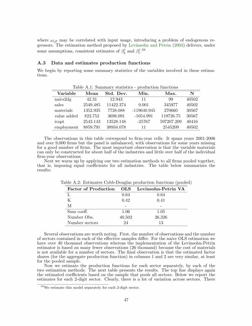
where ωijt may be correlated with input usage, introducing a problem of endogenous re-gressors. The estimation method proposed by Levinsohn and Petrin (2003) delivers, under

some assumptions, consistent estimates of βjk and βj` .59

A.3 Data and estimates production functions

We begin by reporting some summary statistics of the variables involved in these estima-tions.

Table A.1: Summary statistics - production functions

Variable Mean Std. Dev. Min. Max. N

naics2dg 42.31 12.943 11 99 40502sales 2549.485 11422.374 0.001 345977 40502materials 1352.935 7728.088 -119640.945 270660 30567value added 823.752 3698.091 -1054.991 119726.75 30567icapt 2543.143 13528.148 -25767 597207.209 40416employment 8859.791 38934.078 11 2545209 40502

The observations in this table correspond to firm-year cells. It spans years 2001-2006and over 9,000 firms but the panel is unbalanced, with observations for some years missingfor a good number of firms. The most important observation is that the variable materialscan only be constructed for about half of the industries and little over half of the individualfirm-year observations.

Next we warm up by applying our two estimation methods to all firms pooled together,that is, imposing equal coefficients for all industries. The table below summarizes theresults:

Table A.2: Estimates Cobb-Douglas production functions (pooled)

Factor of Production OLS Levinsohn-Petrin VA

L 0.64 0.64K 0.42 0.41M - -

Sum coeff. 1.06 1.05Number Obs. 40,502 26,326Number sectors 24 13

Several observations are worth noting. First, the number of observations and the numberof sectors contained in each of the effective samples differ. For the naive OLS estimation wehave over 40 thousand observations whereas the implementation of the Levinsohn-Petrinestimator is based on many fewer observations (26 thousand) because the cost of materialsis not available for a number of sectors. The final observation is that the estimated factorshares (for the aggregate production function) in columns 1 and 2 are very similar, at leastfor the pooled sample.

Now we estimate the production functions for each sector separately, by each of thetwo estimation methods. The next table presents the results. The top line displays againthe estimated coefficients based on the sample that pools all sectors. Below we report theestimates for each 2-digit sector. Clearly, there is a lot of variation across sectors. There

59We estimate this model separately for each 2-digit sector.

47

is also a positive correlation (0.20) between the (labor) shares obtained by OLS and bythe Levinsohn-Petrin GMM estimator. However, there are also important differences. Forexample the OLS estimation identifies the Construction sector (23) as the one with thehighest labor share, in contrast the Levinsohn-Petrin approach implies that Professional,Scientific and Technical services (54) is the industry with the highest labor share. Bothfindings are reasonable but these discrepancies are likely to lead to differences in the resultingestimates of TFP.

Table A.3: Estimates Cobb-Douglas production functions (by sector)

Estimation OLS OLS Levinsohn-Petrin Levinsohn-PetrinFactor Labor Capital Labor Capital

Pooled 0.64 0.42 0.64 0.40

Sector11 0.56 0.4721 0.38 0.7222 0.47 0.4823 0.92 0.08 0.60 0.4931 0.66 0.27 0.58 0.3732 0.88 0.30 0.60 0.3833 0.84 0.20 0.75 0.4842 0.79 0.16 0.68 0.5644 0.43 0.45 0.74 0.2845 0.61 0.23 0.74 0.3248 0.56 0.2849 0.75 0.1251 0.82 0.21 0.70 0.3852 0.89 0.17 0.73 0.3153 0.57 0.2954 0.88 0.15 0.92 0.2555 0.64 0.4256 0.53 0.34 0.75 0.2261 0.27 0.4362 0.71 0.20 0.72 0.2871 0.48 0.39 0.52 0.5972 0.69 0.28 0.70 0.2681 0.53 0.24 0.66 0.47

Several observations are worth noting. First, the table has many gaps. This correspondsto the sectors for which the cost of materials is missing.60 We fill all these gaps using theestimated coefficients obtained on the pooled sample, using the appropriate estimationmethod in each case.

60For sector 55 the naive OLS estimation delivers a negative capital share, which does not make sense sowe drop those estimates.

48

A.4 Construction of TFP

On the basis of the sector-specific estimates for the coefficients of the production functionswe now build firm-year TFP measures as a residual. Specifically, for the naive OLS methodwe do the following:61

TFP 1ijt = εijt = yijt −

ˆβjkkijt −

ˆβj` `ijt. (25)

For the Levinsohn-Petrin estimates we compute

TFP 2ijt = εijt = vijt −

ˆβjkkijt −

ˆβj` `ijt. (26)

We next compute the 2001-2006 log difference for each of these measures, which is ourfocus on interest. The correlation coefficients among the log changes for these variables isaround 0.40. The advantage of the first measure (naive estimation) is that we can computeit for all firms in the sample, spanning 24 sectors. The measures based on the Levinsohn-Petrin estimation have a stronger theoretical and econometric foundation. However, theyare missing for about half of the firms in our final sample.

B Alternative measure of dependency on H-1B visas

The Tables that follow are part of the discussion in Section 8. Briefly, we experiment with analternative measure of dependency on H-1B visas. Specifically, we follow Kerr and Lincoln(2010) and use the number of LCAs filed in 2001 normalized by total employment in thefirm, whereas, in our main analysis, we have used the total number of LCAs filed by a firmin year 2001.

61We do not include the estimated intercept in the construction of the TFP value for each firm-yearobservation. Since our focus is on changes in TFP over time for a given firm this will not affect our results.

49

Table B.1: Industry results - Alternative dependency measure

(1) (2) (3) (4) (5) (6)Dep. var. is ∆ ln of Sales

Emp Sales Emp Profits TFP 1 R&D

Sample: All firms (N=3,945)∆H1B ×D{0 ≤LCA01/Emp01≤ p80} -0.27 0.44 0.71*** 0.71** -0.26 0.22

[0.25] [0.31] [0.25] [0.30] [0.23] [0.49]∆H1B ×D{p80 ≤LCA01/Emp01≤ p90} -0.11 0.11 0.21 0.51 -0.39 0.66

[0.91] [1.09] [0.83] [0.98] [0.92] [1.05]∆H1B ×D{LCA01/Emp01≥ p90} -0.76 -1.51 -0.75 -0.15 -0.45 -0.37

[1.00] [1.22] [0.99] [1.49] [0.92] [1.24]Sample: R&D (N=969)∆H1B ×D{0 ≤LCA01/Emp01≤ p80} 0.06 0.53 0.47 0.51 0.23 0.26

[0.46] [0.57] [0.37] [0.50] [0.47] [0.42]∆H1B ×D{p80 ≤LCA01/Emp01≤ p90} 0.15 0.74 0.59 1.10 -0.04 1.91**

[1.28] [1.58] [0.85] [1.36] [1.30] [0.97]∆H1B ×D{LCA01/Emp01≥ p90} -1.50 -0.74 0.76 -2.97 -1.92 1.91

[1.35] [1.61] [1.15] [2.02] [1.46] [1.33]Sample: Manufacturing (N=1,549)∆H1B ×D{0 ≤LCA01/Emp01≤ p80} -0.55 0.26 0.82** 1.02** -0.63 0.56

[0.42] [0.49] [0.35] [0.43] [0.42] [0.44]∆H1B ×D{p80 ≤LCA01/Emp01≤ p90} -1.56 0.41 1.97 2.22 -2.37 3.40***

[1.69] [1.92] [1.24] [1.79] [1.73] [1.23]∆H1B ×D{LCA01/Emp01≥ p90} -1.16 -0.72 0.43 -0.94 -1.64 1.53

[1.67] [2.11] [2.13] [2.93] [1.74] [1.66]

Heteroskedasticity-robust standard errors in brackets*** p<0.01, ** p<0.05, * p<0.1

Notes: The omitted category are firms with zero LCAs in 2001. All regressions include 2-digit sector dummyvariables. The first panel contains the whole sample of firms. The second panel is the R&D subsample. Thethird panel is the subsample of manufacturing sectors (NAICS 31-33).

Table B.2: Linear Model with Kerr-Lincoln sample - Alternative dependency measure

(1) (2) (3) (4) (5)

Dep. var. is ∆ ln of SalesEmp Sales Emp Profits R&D

∆H1B × LCA2001 0.09 0.23 0.14 0.11 0.23[0.08] [0.35] [0.32] [0.21] [0.39]

∆H1B × LCA2001/Emp2001 4.03 -8.02 -12.05 3.31 -13.46[8.44] [23.00] [20.92] [31.02] [24.47]

Observations 99 99 99 98 99

Notes: All regressions include 2-digit sector dummy variables. The sample contains firms with at least 60LCAs in year 2001 with R&D expenditures in both 2001 and 2006 of at least $5,000.

50