The Impact of Price Caps and Spending Cuts on

U.S. Postsecondary Attainment

David J. Deming

Harvard University and NBER

Christopher R. Walters

UC Berkeley and NBER∗

August 2017

Abstract

Increasing the postsecondary attainment rate of college-age youth is an important economic priority

in the U.S. and in other developed countries. Yet little is known about whether different forms of

public subsidy can increase degree completion. In this paper, we compare the impact of the marginal

taxpayer dollar on postsecondary attainment when it is spent on lowering tuition prices versus increasing

the quality of the college experience. We do so by estimating the causal impact of changes in tuition

and spending on enrollment and degree completion in U.S. public postsecondary institutions between

1990 and 2013. We estimate these impacts using a newly assembled data set of legislative tuition caps

and freezes, combined with variation in exposure to state budget shocks that is driven by differences

in historical reliance on state appropriations. We find large impacts of spending on enrollment and

degree completion. In contrast, we find no impact of price changes. Our estimates suggest that spending

increases are more effective per-dollar than price cuts as a means of increasing postsecondary attainment.

∗Emails: david_deming@harvard.edu; crwalters@econ.berkeley.edu. Thanks to John Bound, Susan Dynarski, Mark Hoek-stra, Jesse Rothstein, Kevin Stange, Lesley Turner, Sarah Turner and seminar participants at Northwestern University, the UCBerkeley Goldman School of Public Policy, William & Mary, the University of Toronto, the Brookings Institution, the 2016 and2017 American Economic Association Annual Meetings, and the 2016 APPAM Fall Conference for helpful comments. OliviaChi, Patrick Lapid, and Tomas Monarrez provided superb research assistance.

1

1 Introduction

Postsecondary attainment rates across countries and sub-country regions are strongly related to economic

growth (Hanushek and Woessmann, 2008; Gennaioli et al., 2013; Hanushek et al., forthcoming). Yet the

share of college-educated youth in the U.S. has grown only slowly over the last several decades, compared to

more rapid growth rates in other developed countries (OECD, 2013; Autor, 2014). Thus increasing degree

completion rates among U.S. college-age youth is an important national economic priority.

College costs are frequently cited as a key reason for the slow growth of U.S. educational attainment,

and tuition and fees at U.S. public institutions have risen much faster than the rate of inflation over the last

thirty years (Dynarski, 2008; Deming and Dynarski, 2010; Baum and Ma, 2014). The Federal government

has responded to rising college prices by tripling expenditures on Federal financial aid between 1995 and

2015, from $50 billion to over $150 billion in constant 2015 dollars, and many U.S. states introduced state

merit aid scholarships and need-based aid programs over the same period (Dynarski, 2008; Fitzpatrick and

Jones, 2012; Baum and Ma, 2014).

Yet despite dramatic increases in financial aid, the share of U.S. youth age 25-29 who complete a bachelor’s

degree or higher has risen only modestly in recent years, from 27.9 percent in 2000 to 30.2 percent in 2013

(National Center for Education Statistics, 2015a). Why have large increases in financial aid not led to large

increases in college degree attainment? One possibility is that college quality has declined. Between 2000

and 2014, inflation-adjusted state appropriations per full-time equivalent student fell by 28 percent, and

total per-student spending fell by 16 percent (Baum and Ma, 2014).1

While there is a strong positive correlation between per student spending and rates of degree completion

in U.S. public postsecondary institutions, there exists little causal evidence of the impact of changes in per-

student spending on degree completion (e.g. Bound and Turner, 2007; Deming, 2017). One view is that higher

education spending pays for administrative bloat and consumption amenities, in which case lower levels of

spending may be cost-effective (see, e.g., Ginsberg, 2011; Ehrenberg, 2012; and Jacob et al., 2013). On the

other hand, spending cuts may reduce degree completion by harming the quality of instruction, limiting

the number and variety of course offerings, increasing class size, or moving students into non-credit-bearing

remedial courses (Bettinger and Long, 2009; Bahr, 2014).

We use data from the Integrated Postsecondary Education Data System (IPEDS) to study the impact

of changes in spending and tuition at U.S. public postsecondary institutions between 1990 and 2013. The

thought experiment that motivates our analysis is as follows. Suppose a U.S. public institution receives an

unexpected increase in state appropriations of $1,000 per student. One option is to pass this extra $1,000

on to students in the form of tuition cuts or scholarships. This would reduce the price of college, but keep

per-student spending constant. Alternatively, the college might elect to keep tuition constant and spend the

1Authors’ calculations using the Integrated Postsecondary Education Data System (IPEDS). Another possible reason fordeclining college attainment rates is that recent cohorts of students are less academically prepared for college. Yet math andreading achievement levels of U.S. students have remained constant or even increased slightly in recent years (National Centerfor Education Statistics, 2015b).

2

extra $1,000 per student on smaller classes, fancier athletic facilities, or other educational inputs or amenities.

We seek to determine which of these choices would lead to a larger impact on student enrollment and degree

completion. In other words, if the goal is increasing postsecondary attainment, should the marginal public

dollar be spent on lowering tuition prices or increasing college quality?

Our analysis exploits cross-sectional variation in institutions’ historical reliance on state appropriations

combined with state-level changes in funding over time to identify impacts of state funding on spending,

tuition and enrollment. State appropriations for higher education fluctuate with the business cycle, and

policy decisions about higher education funding generally operate at the state level (Kane et al., 2003; Barr

and Turner, 2013). Yet the impact of a state-level budget cut is likely to be greater for institutions that rely

more heavily on state appropriations as a source of revenue. This idea motivates an instrumental variables

(IV) strategy that uses the interaction between total state appropriations for higher education and each

institution’s baseline dependence on state support to instrument for state funding. Our IV strategy discards

variation in funding driven by policymakers’ decisions about which institutions to support in particular years,

and allows us to control for permanent differences across institutions, changes in outcomes common to all

institutions within a state, and important time-varying determinants of the demand for higher education

such as state and local unemployment rates. This approach parallels identification strategies commonly

used in studies of local labor markets, immigration, and trade, which also construct instruments combining

cross-sectional exposure with aggregate changes in the treatment of interest (Bartik, 1991; Blanchard and

Katz, 1992; Card, 2001; Autor et al., 2013).

Schools can respond to budget cuts by reducing spending or raising tuition. The reduced form effect of a

budget shock on enrollment measures the net impact of adjustments on both margins. Identification of the

partial effects of prices and spending requires an additional instrument that induces independent variation in

these two variables. To this end, we construct instruments for tuition using a newly assembled data source

of tuition caps and freezes imposed by state legislatures. Using the budget shock and price cap instruments

together in a two-stage least squares (2SLS) framework allows us to separately estimate the impact of a price

change holding spending constant, and a spending change holding price constant.

We find large impacts of spending on student enrollment. Our estimates imply that a 10 percent increase

in spending increases current enrollment by 3 percent. In contrast, estimated impacts of price changes are

statistically insignificant. While we cannot reject modest price elasticities, our estimates are precise enough

to reject equal elasticities of enrollment with respect to prices and spending at the five percent level. We

find positive and statistically significant impacts of spending on enrollment for both two-year and four-year

institutions, although the elasticites for two-year institutions are somewhat larger.

We also find positive and statistically significant causal impacts of spending on degree completion, in-

cluding bachelor’s degrees. Our estimates imply that the marginal cost of an additional bachelor’s degree

is between $102,532 and $155,451, an effect that passes a benefit-cost test under conservative assumptions

about the private labor market returns to college completion. We present evidence that spending impacts are

3

driven mostly by increased persistence and degree completion among already-enrolled students, rather than

increases in initial college matriculation. We also find that only about 15 percent of the enrollment impact

of spending at public institutions can be explained by crowd-out of private school enrollment. Moreover,

while do we find some evidence of significant crowdout for associate’s degrees, increased public funding of

postsecondary institutions appears to increase total certificate and bachelor’s degree completion, rather than

simply shifting students across sectors. Finally, we find no evidence that price or spending changes affect

financial aid, suggesting that changes in sticker price also lead to changes in the net price paid by students.

To our knowledge, this is the first paper to directly demonstrate a causal link between spending and

degree attainment in U.S. postsecondary institutions. The most closely related paper is Bound and Turner

(2007), who show that larger state cohorts have lower degree attainment rates. While they argue that lower

public subsidies per student are the key causal mechanism, they do not directly measure changes in public

spending on higher education, nor do they use institution-level data on student outcomes. More broadly,

our results relate to studies of “cohort crowding” and college quality, which draw linkages between changes in

college resources, declining completion rates and increased time to degree over the last twenty years (Turner,

2004; Dynarski, 2008; Bound and Turner, 2007; Bound et al., 2010, 2012).

We find that changes in state funding lead to large impacts on core academic spending. Instruction alone

accounts for about 40 cents of every dollar increase in spending. Moreover, we find that academic support

spending - including tutoring, advising and mentoring - is particularly responsive to state budget shocks.

This is consistent with a number of recent studies finding large impacts of student supports on persistence

and degree completion (Angrist et al., 2009; Bettinger and Baker, 2011; Carrell and Sacerdote, 2013; Barrow

et al., 2014; Scrivener et al., 2015). While ultimately the mechanisms are only suggestive, we argue that

our results are most consistent with spending improving quality by lifting informal capacity constraints such

as course waitlists and inadequate advising (e.g. Bound et al., 2012).2 Further afield, our findings are

also consistent with evidence that increased resources at primary and secondary schools boost educational

attainment and other outcomes (Card and Krueger, 1992; Jackson et al., 2016; Lafortune et al., 2016).

The rest of the paper proceeds as follows. Section 2 describes the data and provides some background

information on the state higher education budgeting and tuition regulation processes. Section 3 lays out

our identification strategy for estimating causal effects of spending and tuition, and explores the validity of

our approach. Section 4 presents our main results - estimates of the effects of price and spending changes

on enrollment and degree completion. Section 5 describes additional results and discusses some policy

implications of our findings. Section 6 concludes.

2In principle, spending cuts could lead to formal capacity constraints through admissions quotas. We think this is unlikelyto explain our results, for two reasons. First, most of the colleges in our sample (and nearly all of the community colleges)accept every student who applies and meets minimum academic qualifications. Second, a web search revealed the existence offormal capacity constraints in only a handful of states and years. Our results are robust to excluding schools that accept fewerthan 50 or 75 percent of applicants, and they are nearly unchanged when we exclude states and years with formal capacityconstraints from the analysis.

4

2 Data and Background

2.1 Data Description

The data used here come from the Integrated Postsecondary Education Data System (IPEDS). IPEDS is

a survey of colleges, universities and vocational institutions conducted annually by the U.S. Department of

Education (DOE). The Higher Education Act requires postsecondary institutions to participate in IPEDS

to retain eligibility to administer Federal Title IV student aid (Pell Grants and Stafford Loans).3 IPEDS

collects information on student enrollment overall and by race, gender, age and student status (part-time/full-

time, freshman/continuing student, undergraduate/graduate, degree-seeking), as well as degree completion

by level (certificate, associate’s, bachelor’s) and field of study. IPEDS also collects detailed information on

institutional finances, including revenues and expenditures by source. IPEDS data on all variables relevant

for our study are available back to 1990.

IPEDS collects data at the campus level using a unique longitudinal identifier, and includes basic infor-

mation about each campus such as level, control, degree-granting status and geographic location. Campus-

level data allows us to separate enrollment and finances for branch campuses of university systems.4 We

supplement the IPEDS data with state legislative appropriations data from Grapevine, an annual survey

compilation of data on state support for higher education administered by the State Higher Education Ex-

ecutive Officers (SHEEO) Association and the Center for the Study of Education Policy at Illinois State

University.5 We also match the IPEDS to publicly available data on state and county unemployment rates

collected by the Bureau of Labor Statistics, as well as annual data on state tax receipts and other forms of

state government spending such as Medicaid. Finally, we match IPEDS to state- and county-level data from

the Census and the American Community Survey (ACS).6

Table 1 presents descriptive statistics for our analytic sample. The first ten rows display financial in-

formation for public institutions by sector and selectivity. Selective public four-year universities are those

ranked “Most Competitive” or “Highly Competitive” - the two highest categories - in the 2009 Barron’s Profile

of American Colleges. All financial data are in per-student terms, weighted by enrollment and adjusted for

3Postsecondary institutions that do not administer Title IV aid are not required to report to IPEDS. There are many ofthese institutions, but they are very small and generally offer non-degree certificate programs and other short courses. Nearlyall non-Title IV institutions are for-profit - see Cellini (2010) for a more detailed discussion.

4To ensure the accuracy and consistency of our data over time, we compare the raw IPEDS data to data from the Delta CostProject (DCP), a collaboration between the DOE and the American Institutes for Research that makes IPEDS longitudinallyconsistent and matches branch campuses of individual institutions together. Jaquette and Parra (2016) show that the DCPdatabase collapses multiple institutions within some public university systems into a single administrative unit, which would beproblematic for our analysis. We therefore use the raw IPEDS data rather than the DCP, although results are generally similarin either case.

5The Grapevine data can be found at https://education.illinoisstate.edu/grapevine/historical/. We measure appropriationsfrom Grapevine rather than IPEDS because of concerns about duplicate reporting of state funding across campus branches ofinstitutions, as well as errors in administrator survey responses. IPEDS appropriations aggregated to the state-year level aresimilar to corresponding measures in Grapevine (the correlation equals 0.83).

6County identifiers appear in the IPEDS from 1990 to 1999, and then again from 2008 onward. For over 95 percent ofinstitutions and 99 percent of publics, county codes were consistent in 1999 and 2008, and alternative measures of geography(MSA, address, city, zip code) also did not change. In these cases we interpolate county IDs for the intervening years. In thesmall number of cases where location changed or was missing, we use other institutions with the same alternative geography tofill in missing values. Geographic information is left missing in cases where we cannot reliably locate an institution.

5

inflation using the Higher Education Price Index. Financial data are collected as of the fiscal year, which

usually begins in July. Enrollment data are counted for the fall of each calendar year.

The sample is restricted to institutions in the 50 U.S. states (excluding Puerto Rico) and excludes schools

with missing values for state appropriations in 1990. To address concerns about reporting and measurement

error in IPEDS spending data, we also eliminate the less than 3 percent of institutions with per capita

spending of less than $100 or more than $100,000 per college-age student in any year in the panel. Note

that total spending includes capital costs such as operation and maintenance in addition to core academic

functions.

Table 1 reveals four key facts. First, per-student spending in public institutions derives largely from three

sources: state (and local) appropriations, tuition and fees, and financial aid grant programs (mainly Federal

Pell Grants, but also including state and local grants). This is particulary true for less selective schools.

In 1990, the combined contributions of these three categories to total spending at selective four-year, less

selective four-year, and two-year institutions equaled 64, 78 and 90 percent, respectively. The relatively small

contributions of other categories such as endowment spending means that budgets are strongly affected by

cuts in state funding, especially for less selective institutions.

Second, more than half of total spending is accounted for by the core categories of instruction, academic

support, and student services, and the share of total spending devoted to these core categories has grown

over time. Core academic spending is a higher share of total spending for less selective institutions. Third,

while less selective schools receive much lower levels of state funding in dollar terms, they rely more heavily

on state support. In 1990, state and local appropriations represented about 44 percent of total spending for

selective four-year institutions, compared to 51 percent for less-selective four-year institutions and 62 percent

for two-year institutions. This means that a state budget cut should have greater relative impacts on less

selective institutions. Fourth, all types of public institutions received less public support and became more

reliant on tuition revenue between 1990 and 2013.

2.2 Higher Education Appropriations and Tuition

Our description of state legislative higher education funding relies on a SHEEO survey of state budgetary

processes (Parmley et al., 2009). While the details differ across states, a typical budgetary process unfolds

as follows:7

1. One to two years in advance of the fiscal year, a state higher education coordinating board develops a

budget request that covers all public institutions in the state.

7The SHEEO survey, which received responses from 43 states, covers topics such as how budget requests are developed, howfunds are administered across campuses, and which organizations have primary authority over spending and tuition setting.All but one surveyed state had a coordinating board of some kind. Institutions submit budget requests individually in onlysix states. Most respondents indicated that budget requests are based on past and future projections of enrollment, changesin costs such as salaries, and any special projects or initiatives. In 14 cases, respondents indicated that governors vetoed orreduced specific budget line items. The executive branch fully funded the initial budget request in about half of cases, and thatnumber is slightly lower for the legislative budget. Open-ended responses to the survey indicated that economic conditions andother legislative priorities were key reasons that higher education budget requests were not fully funded.

6

2. The governor proposes a budget based on the request. The legislature then enacts its preferred budget,

and the governor can subtract individual items or veto the budget entirely, while the legislature can

accept (or override in some cases) the modified budget. Protracted negotiations are common and can

become quite complicated.

3. The end result is a budget that is typically ratified in the spring and takes effect the following fall. A

key source of uncertainty in this process is the possibility that budget requests will not be fully funded,

and this is especially likely when tax revenues are less than expected.

An important difference between state and Federal budgeting processes is that states are mostly unable

to smooth business cycle fluctuations in tax revenue. Nearly all states have some sort of balanced budget

requirement, and higher education spending often serves as the “balance wheel” used to meet these require-

ments when tax revenues fall short of projections (Kane et al., 2003; Delaney and Doyle, 2011; Barr and

Turner, 2013).

States differ markedly in their support for higher education. Appendix Figure A1 presents trends in per

capita approprations in four large states. The figure shows substantial differences in levels of funding and in

trends over time. For example, in California real per-capita state appropriations for higher education grew

from around $5,000 in 1990 to over $6,000 in the early 2000s, before plummeting to less than $4,000 in 2013.

In contrast, public support for higher education in Texas remained roughly constant at around $4,000 per

student over this period. These heterogeneous patterns are typical of the wide variation in public higher

education spending across states, even those with similar demographics.8

State policies influence both spending and tuition at public institutions. As noted by Bell et al. (2011),

states vary in the extent of legislative control over tuition setting.9 Tuition setting is generally less centralized

than the state appropriations process, with institutions setting tuition either completely on their own or in

non-binding consultation with the higher education coordinating board. However, state legislatures can

exert formal control over prices through tuition caps, defined as statutory limits on increases in public

college tuition from one year to the next. Tuition caps affect higher education budgets by shutting down one

margin of adjustment. Institutions operating under a legislative tuition cap cannot respond to appropriations

shocks by increasing prices, and thus are more likely to cut spending.

Seventeen states imposed formal price controls on public institutions at least once between 1990 and 2013.

The complete list appears in Appendix Table A1. We compiled these data by referencing official sources

when available, combined with Lexis-Nexis searches of state newspapers going back to 1990. Some states

8For example, appropriations per capita were about 50 percent higher in New Mexico compared to Arizona, and that gaphas widened considerably since 2010. Arkansas, Tennessee and Kentucky all spent about $3,100 per capita in 1990. In the early2000s Kentucky had the highest per capita spending (around $5,600, compared to $4,300 in Arkansas and $3,500 in Tennessee),but by 2013 Arkansas was spending the most ($5,500, compared to $4,700 in Kentucky and only $3,000 in Tennessee).

9Bell et al. (2011) describe a SHEEO survey of tuition, fee and financial assistance policies, which received responses from35 states. Only four states indicated that formal tuition-setting authority for either the two-year or four-year sector lies withthe legislature. In nearly all other states, tuition is set by the coordinating board in consultation with individual institutions,and changes in tuition are not necessarily uniform across institutions. In all but six of the states that responded, tuition revenueis controlled and retained by individual campuses.

7

impose uniform tuition caps, while others single out particular sectors or even institutions. Tuition caps

appear to be more frequent in economic boom times (e.g. 1994-2000, 2006-2009), but there is no obvious

geographic or demographic pattern in which states impose price caps. The five states with the highest

(enrollment-weighted) exposure to tuition caps are Ohio, Idaho, Virginia, New York and Maryland. Across

all years in our sample, about 9 percent of students were enrolled in public institutions operating under a

legislative tuition cap or freeze.

2.3 Naive Estimates of Enrollment Impacts

Reverse causality is the central challenge in estimating the impacts of price and spending changes on enroll-

ment. Policymakers might award additional funding and push for lower prices in colleges that are already

expanding their enrollment - perhaps because of increasing local demand for higher education. Changing

demand would lead to reverse causality, with enrollment affecting tuition prices rather than tuition prices

affecting enrollment. Similarly, spending may increase in anticipation of growth in demand, and increased

enrollment tends to generate higher tuition revenue and therefore more spending.

To illustrate this concern, we show how naive estimates of enrollment impacts are biased by reverse

causality. Consider the following panel regression of enrollment on spending or tuition:

Yi,t = γi + ψt +

L∑`=−L

δ`Xi,t−` + ui,t, (1)

where Yi,t represents log enrollment for institution i in year t, γi and ψt are institution and year fixed effects,

and Xi,t is log total spending or log tuition. The coefficient δ` describes the relationship between enrollment

in year t and tuition or spending ` years earlier, controlling for permanent differences across institutions,

changes over time common to all institutions, and tuition or spending in other years. Standard errors are

clustered by institution.

Figure 1 plots estimates of equation (1), with coefficients arranged in event time so that positive indices

correspond to lagged spending and tuition. The top panel shows results for log spending. Spending increases

are correlated with contemporaneous increases in enrollment. The base year coefficient suggests that a 10

percent increase in spending in year t is associated with a 3.0 percent increase in enrollment in this year.

Current spending is also associated with smaller increases in enrollment in subsequent years. The bottom

panel shows results for log tuition. A 10 percent tuition cut in year t is associated with a 0.24 percent

enrollment increase in the same year. This estimate is somewhat smaller than estimates reported by Hemelt

and Marcotte (2011), a study that uses a similar panel framework with additional controls and finds an

elasticity of enrollment with respect to tuition equal to -0.08 for non-selective public institutions.

However, the bottom panel of Figure 1 shows that higher tuition in year t+ 1 is associated with higher

enrollment in year t, which suggests that institutions lower tuition both before and after increases in en-

rollment. Likewise, we find a statistically significant and positive pre-trend coefficient for the association

8

between spending in year t+ 1 and enrollment in year t. Overall, the patterns in Figure 1 suggest that while

enrollment tends to change contemporaneously with spending and tuition, naive regressions of enrollment

on changes in spending and price should not be interpreted causally.

A possible solution to this endogeneity problem is to study changes in spending and prices that are

induced by state-level policy changes. Figure 2 presents estimates of equation (1) with log total spending,

log tuition and log enrollment as the dependent variables, and log state appropriations as the key right-hand

side variable. As above, these models include institution and year fixed effects.

The top panel shows that state appropriations are strongly linked to current spending. A 10 percent

increase in appropriations in year t is associated with a 3.1 percent increase in spending in the same year.

The middle panel shows that state funding is negatively correlated with tuition prices, with a 10 percent

increase in appropriations linked to a price cut of about 0.6 percent. However, the bottom panel indicates

that while increases in appropriations are linked to contemporaneous and later increases in enrollment, there

is evidence of significant pre-trends.

Figure 2 shows that there are at least two problems with using changes in state appropriations to estimate

the impacts of spending on college enrollment. First, as shown in the bottom panel, future appropriations

changes predict current enrollment. This pattern may reflect funding decisions that anticipate changes in

the demand for higher education. For example, state legislatures may allocate more total funds for higher

education when enrollment is projected to grow quickly, or target extra funds to institutions within a state

where demand is growing especially fast.

A second problem highlighted by Figure 2 is that even exogenous changes in state funding would not be

sufficient to identify the effects of spending and tuition on enrollment. The top and middle panels show that

institutions appear to adjust both spending and tuition in response to higher appropriations. The impact

of an increase in state funding therefore measures the combined effect of both potential adjustments. This

simultaneity between spending and price responses complicates the interpretation of studies that seek to

study the effects of tuition or school resources in isolation (e.g., Hemelt and Marcotte, 2011). In the next

section, we develop an instrumental variables strategy that combines a plausibly exogenous component of

state funding with price variation from legislative caps and freezes to separate the impacts of spending and

tuition.

3 Identification Strategy

3.1 Budget Shocks and Tuition Caps

As discussed above, state budget changes are typically - but not always - made “across the board” (e.g.

all institutions in the state receive 90 percent of their funding requests).10 However, an across the board

10Despite the multiple rounds of negotiation and attention to specific line items, more than half of respondents to the 2009SHEEO survey indicated that appropriations are distributed as lump sum amounts rather than individual line items that areearmarked for a particular use (Parmley et al. 2009). In some cases, appropriations are distributed to the coordinating board

9

budget cut is likely to have a greater proportionate impact on institutions that rely on state appropriations

for a larger share of operating revenue. Thus some schools’ budgets are more sensitive to state-level funding

fluctuations than others. We exploit ex ante differences across institutions in their reliance on state revenue

to estimate the impact of funding changes.

Specifically, we construct a budget shock instrumental variable (IV) that multiplies yearly state appro-

priations by each public institution’s share of total revenue from state appropriations in 1990, the first year

that IPEDS data are available. This instrument is constructed as

Zi,t =

(Appropi,90Revi,90

)×(StApprops(i),t

Pops(i),t

), (2)

where Appropi,90 and Revi,90 measure state appropriations and total revenue for institution i in 1990, s(i)

denotes state for institution i, and StApprops,t and Pops,t represent total appropriations and college-age

population for state s in year t. The first factor in (2) is each institution’s revenue from state appropriations

divided by total revenue in 1990. This captures a school’s dependence on state funds at baseline. Using

the 1990 revenue shares shuts down variation in exposure to state budget shocks that might be driven by

endogenous institutional responses. For example, institutions might become more or less dependent on state

appropriations over time based on changing selectivity, increased ability to attract out-of-state students, or

other sources of unobserved heterogeneity.

The second factor in (2) calculates state appropriations per college-age (age 19-23) student in each

state and year, using Grapevine data rather than institution-level appropriations from IPEDS. Restricting

variation in state appropriations to the state-year level addresses the concern that schools receiving more or

less funding within a particular state and year may differ in unobserved ways. For example, a budget cut

for an individual institution may be more or less severe depending on the current political influence of its

leadership. State legislatures might allocate additional funds to colleges in labor markets that have been hit

particularly hard by economic downturns.

Our second source of identifying variation leverages legislatively imposed tuition caps and freezes. We use

the information in Table A1 to code two instruments related to tuition caps. The first, TuitCapi,t, equals

one if institution i is subject to a cap or freeze in year t. The second, TuitMaxi,t, equals the maximum

percentage increase allowed by the state legislature between years t− 1 and t for institution i. For example,

this variable equals zero for institutions subject to tuition freezes, and 0.1 for institutions where tuition

growth is constrained to no more than 10 percent. We include both of these variables in our estimating

equations and code TuitMaxi,t to zero for cases where TuitCapi,t = 0. Thus the coefficient on TuitCapi,t

can be interpreted as the impact of a tuition freeze, i.e. when the maximum percentage increase allowed

equals zero. The combination of these two variables allows us to exploit variation in both the existence and

intensity of tuition cap legislation.

to disburse to schools, while in other cases funding goes directly to schools.

10

To get a sense for which colleges are most affected by state budget shocks, Appendix Table A2 presents

estimates of the correlation between institutional characteristics and baseline dependence on state appro-

priations (the first term in Zi,t above) in a regression framework. Four-year, less-selective institutions are

most reliant on state appropriations, for two reasons. First, many two-year colleges also receive funding

from property taxes and other local sources. Second, selective four-year institutions are generally larger

and have other sources of revenue such as research grants and endowment spending. Dependence on tu-

ition revenue is also positively correlated with dependence on state appropriations, which is consistent with

less-selective institutions having fewer margins of adjustment in response to a budget shock. Finally, larger

institutions (as measured both by total spending and enrollment) draw a lower share of total revenue from

state appropriations.

3.2 Assessing the Validity of the Instruments

We explore the validity of the instruments by testing for pre-trends with the following reduced form model:

Yi,t = αi + µt + ζs(i) × t+W ′i,tθ +

L∑`=−L

[ρZ` Zi,t−` + ρC` TuitCapi,t−` + ρM` TuitMaxi,t−`

]+ vi,t. (3)

The vector Wi,t includes state and county unemployment rates by year, time-varying institution charac-

teristics such as highest degree offered and eligibility to distribute Federal financial aid, county average

demographic and economic characteristics, and interactions of these variables with time.11 We also control

for state-specific linear time trends, represented by ξs(i) × t. Standard errors for this analysis are clustered

at the state-year level. Here and in our subsequent results, we divide Zi,t by 1,000 for ease of interpreta-

tion. The coefficients on the leads of the policy variables check whether there are differential prior trends in

outcomes for institutions that later experience differential changes in the instruments. Our baseline model

includes 4 leads and 5 lags of each instrument and both unemployment rates (for ten years total), although

our results are not sensitive to this particular number of years.

Figure 3 presents estimates of equation (3) for log enrollment, our key outcome of interest. The top panel

shows coefficients and 95 percent confidence intervals for the budget shock instrument, while the middle and

bottom panels show results for the tuition cap indicator and the maximum tuition increase. In contrast

to the results using actual appropriations in Figure 2, we find no evidence of pre-trends in the relationship

between the budget shock and log enrollment. The coefficients on all four leads are precisely estimated, near

zero and not statistically significant. We fail to reject the hypothesis that all four pre-trend coefficients are

jointly equal to zero (p = 0.64). Additionally, we find a positive impact of the budget shock on log enrollment

11The institutional covariates are sector, highest degree offered, Title IV eligibility, degree-granting status, urban status andindicators for missing values of these covariates in each year. These covariates rarely change within institutions over time, butwe include them for completeness. The county covariates are log population, percent black, percent hispanic, percent male,percent below the poverty line, log median income, share with some college education, and share with bachelor’s degree. Countycovariates are only available from the U.S. Census for 1990 and 2000, and from the ACS for 2005 and onward. To complete thecounty data, we linearly interpolate values for missing years.

11

in the same year. This estimate, which is statistically significant at the one percent level, implies that a

$1,000 increase in the instrument increases enrollment in year t by 2.8 percent. We also find statistically

significant and positive impacts of the budget shock on enrollment in future years.

The second and third panels of Figure 3 show no evidence of pre-trends in the relationship between

the tuition cap instruments and log enrollment. All of the pre-trend coefficients are close to zero and

statistically insignificant, and we fail to reject the joint hypothesis that they are jointly equal to zero in both

cases (p = 0.73 and 0.47 for the tuition cap indicator and maximum tuition increase). Unlike the budget

shock, however, we find no reduced form impact of tuition caps on log enrollment.

Figure 4 repeats the exercise above for another key outcome - the log of total degrees and certificates

awarded. While the contemporaneous impact of the budget shock instrument on degrees and certificates is

small, we find a large and statistically significant and positive impacts of a budget shock in year t on log

awards in year t + 1. Moreover, the post-shock coefficients are mostly positive, and we can strongly reject

the joint hypothesis that the coefficients on degrees and certificates in years t through t + 5 all equal zero

(p = 0.001). Additionally, we fail to reject the joint hypothesis that the pre-trend coefficients are equal to

zero (p = 0.35), and there is no visual evidence of pre-trends. As with enrollment, the middle and bottom

panels of Figure 4 show no consistent impact of tuition caps on total awards. While there is some evidence

of a negative impact of a tuition freeze in later years, we fail to reject the hypothesis that all coefficients in

years t through t + 5 equal zero (p = 0.17). Together, the results in Figures 3 and 4 show that our policy

instruments are unrelated to pre-trends in key outcomes.12

The analysis to follow uses budget shocks and tuition caps as instruments for tuition and spending. To

explore the first stage relationships underlying this strategy, Figures 5 and 6 present estimates of equation

(3) for log total spending and log tuition. The top panel of Figure 5 shows clear evidence that the budget

shock IV affects total spending. The coefficients in Panel A imply that a $1,000 increase in the instrument

increases spending in year t by 6 percent. We also find smaller but still statistically significant impacts on

spending in the second and fifth years following the budget shock.

The middle and bottom panels of Figure 5 show some evidence that tuition caps affect spending. However,

we also find negative coefficients on the leads of tuition caps and positive coefficients on the leads of the

maximum tuition cap amount, which suggests that the impact of tuition caps on log spending may reflect a

longer-run trend rather than a sharp policy response. This is less worrisome than a pre-trend for enrollment,

because the key exclusion restriction required for our approach is that the instruments are conditionally

uncorrelated with potential enrollment and degree outcomes. Nonetheless, the pre-trends in Figure 5 suggest

that the tuition cap instruments are not as good as random conditional on our control variables. We address

this issue in part by estimating first-differenced models, which focus on sharper yearly changes in the policy

IVs and endogenous variables.

Figure 6 presents results for tuition prices. We find that a $1,000 increase in the budget shock in year

12Figures A2 and A3 assess the sensitivity of these findings to functional form by reestimating equation (3) with enrollmentand awards in levels rather than logs. These analyses yield similar conclusions.

12

t decreases tuition in year t by 4.8 percent and year t + 1 by 5.8 percent. The impact is closer to zero in

subsequent years. This suggests that public institutions may react to state budget cuts in part by increasing

tuition to make up for lost revenue. The middle and bottom panels of Figure 6 show that the tuition cap

instruments have bite: prices are significantly lower following the imposition of a tuition freeze. Moreover,

conditional on the presence of a cap, the level of the cap is strongly predictive of yearly tuition increases.

There is a strong and immediate impact of the instruments in all three panels of Figure 6.13

3.3 Two-stage Least Squares Framework

Public institutions can respond to budget cuts through a combination of price increases and spending cuts.

Tuition caps generate independent variation in tuition prices. Thus we can use the budget shock together

with the price cap instruments to disentangle the causal impacts of spending and tuition. To this end, we

estimate 2SLS models relating changes in outcomes to changes in spending and tuition, instrumented with

policy variables. The first stage equation for log spending is:

4 log spendi,t = φs(i) + ωt + ∆W ′i,tλ+ π14Zi,t + π24TuitCapi,t + π34TuitMaxi,t + ηi,t. (4)

This equation relates the change in spending relative to the previous year to changes in the budget shock

and tuition cap instruments, controlling for state and year fixed effects and changes in covariates. The first

stage equation for changes in tuition replaces the change in log spending with the change in log tuition on

the left-hand side of (4).

The second stage equation is:

4Yi,t = Φs(i) + Ωt + ∆W ′i,tΛ + β1 ∆ log spendi,t + β2 ∆ log tuitioni,t + εi,t, (5)

where ∆ log spendi,t and ∆ log tuitioni,t are predicted changes in log spending and log tuition from the first

stage. Compared to the fixed effects specifications discussed in Section 4.3, the first-differences specifications

in (4) and (5) focus on the impacts of sharp yearly changes in the instruments on the endogenous variables

and outcomes. When using only two years of data, the two approaches are equivalent; in our longer panel, the

first differences model may be less efficient but captures causal effects under less restrictive assumptions. In

general, our results are similar when we estimate 2SLS models in first differences or in levels with institution

fixed effects, year fixed effects and state-specific linear trends as in equation (3).14

13The middle panel of Figure 6 shows some evidence of a pre-trend in the relationship between tuition caps and tuition -but in the opposite direction of the estimated impact of imposing a cap. This suggests that tuition caps may be imposed inresponse to particularly high tuition in a prior year. Since pre-trends can be interpreted as evidence of anticipation effects (e.g.Malani and Reif 2015), one possible concern is that students may time enrollment decisions in response to anticipated pricechanges. We address this concern in two ways. First, we estimate 2SLS models in first differences, which focuses attention onlyon sharp yearly changes in tuition. Second, we address the sensitivity of the differences specification by excluding the first leadand using the difference between the 2nd lead and the base year as the endogenous first stage variable in Section 4. This leavesthe results nearly unchanged.

14Appendix Table A6 presents results with 2SLS models in levels rather than first differences, for log enrollment (our mainoutcome). The results are qualitatively similar - although somewhat larger in magnitude - to our main results.

13

4 Effects of Price and Spending Subsidies

4.1 Two-stage Least Squares Estimates for Enrollment

Table 2 reports first-stage impacts of the budget shock and tuition cap instruments on log spending and

tuition, along with second-stage impacts on log enrollment. The first stage effect of the budget shock on

spending, reported in column 1, equals 0.061. This implies that a $1,000 increase in the instrument increases

total spending by about 6.1 percent. Since mean total spending is about $104 million per year for the

institutions in our analysis sample, a 6.1 percent increase is about $6.34 million in additional spending. In

contrast, the tuition cap variables are weakly related to log spending.

As shown in column 2, a $1,000 increase in the budget shock decreases log tuition by 8.1 percent, or

about $303. Tuition freezes lower in-state tuition by about 3 percent. The stringency of the cap strongly

predicts the size of the tuition change: a ten percentage point increase in maximum tuition growth leads to

a 3 percent increase in tuition. Both instruments are jointly highly statistically significant, and Angrist and

Pischke (2009) partial F -statistics indicate that the instruments generate substantial independent variation

in log tuition and log spending.

The second-stage estimates imply that enrollment is more sensitive to spending than to tuition. As can

be seen in column 3 of Table 2, a 10 percent increase in log spending increases current-year enrollment by

3 percent, and this estimate is statistically significant at the 5 percent level. In contrast, the estimated

elasticity of enrollment with respect to tuition is close to zero and statistically insignificant. The standard

errors allow us to reject impacts of a 10 percent tuition cut larger than about 1.7 percent. We can also

reject that the elasticities of enrollment with respect to tuition and spending are equal in absolute value

(p < 0.01). Importantly, this null result for tuition holds despite the strong first stage predictive power of

the instruments shown in column 2.

4.2 Enrollment Effects Over Time

Table 3 reports impacts on log enrollment for up to three years after changes in tuition and spending.

Columns 1 through 4 report separate estimates for years t through t + 3 based on the 2SLS framework in

equations (4) and (5). Differences for the outcomes here are taken relative to the base year before the policy

variables are measured, so that the specification for year t+ 1 uses Yi,t+1−Yi,t−1 as the dependent variable,

and similarly for other years. Panel A shows results for the full sample of institutions. Overall, we find that

spending increases have larger impacts on enrollment in subsequent years. The coefficient on log enrollment

increases from 0.304 in the base year to 0.796 one year after the change (p<0.001), with modest increases

thereafter. This suggests that the new students induced to attend by changes in state funding persist for

multiple years of enrollment. In contrast, the coefficients on tuition in subsequent years are small, never

statistically significant, and sometimes wrong-signed.

Panels B and C show results separately for two- and four-year institutions. In both cases, we find large

14

and statistically significant impacts of spending on enrolllment, but little or no impact of price. We find

larger impacts of spending at two-year institutions than at four-year institutions. The coefficients in Panel

B for two-year institutions suggest that a 10 percent increase in total spending in year t boosts enrollment

by around 10 percent in years t + 1 through t + 3. Corresponding estimates for four-year institutions are

smaller but still substantial: a 10 percent increase in spending in year t increases enrollment by 2.4 percent

in year t, 4.7 percent in year t+ 1, 6.6 percent in year t+ 2 and 5.7 percent in year t+ 3. All four of these

estimates are statistically significant at the one percent level.

While these estimates are large, it is important to note that they reflect increases in total enrollment-

years, not individual students. If changes in spending induce students to matriculate or to persist through

college, this will increase enrollment counts in multiple years. Additionally, the log differences specification

implies that a spending shock in year t leads to a persistent 8 percent enrollment gain relative to year t− 1,

not continued growth of 8 percent in each subsequent year. A related issue is that spending shocks are

serially dependent, so that changes in state funding are likely to persist for multiple years. We discuss this

issue further in Section 5.

The outcomes in Table 3 capture total fall enrollment, including part-time, non-degree and graduate

students. Appendix Table A3 presents additional results for part-time and full-time undergraduate enroll-

ment. Undergraduates account for about 92 percent of total enrollment in the sample. About 45 percent

of undergraduates are enrolled part-time, and this breaks down sharply by institution type, with 63 percent

of undergraduates enrolled part-time at two-year colleges compared to only 24 percent at four-year colleges.

We find that the large impacts of spending at two-year institutions are driven by increases in part-time

enrollment, while impacts at four-year institutions are due to increases in both part-time and full-time un-

dergraduate enrollment. Moreover, while most of the estimated tuition elasticities are small and statistically

insignificant, Appendix Table A3 shows statistically significant effects of price changes on part-time enroll-

ment at four-year institutions. This is consistent with results reported by Seftor and Turner (2002), a study

that finds greater price sensitivity among older, independent students who are more likely to be enrolled

part-time.

Appendix Table A4 presents enrollment results by race, with nonwhite students (pooled together) in

Panel A and white students in Panel B. Overall, we find very similar impacts of price and spending changes

by student race. Unfortunately, data on degree completion by race is unavailable.

4.3 Impacts on Certificates and Degrees

Table 4 present results for log total awards. Panel A shows results for all institutions, while Panels B and

C present results for two-year and four-year institutions respectively. We find that a 10 percent increase in

total spending in year t leads to only a 2 percent increase in total awards in year t, but larger increases of

7.8, 9.4 and 6.4 percent in years t+1 through t+3, respectively. The impacts on log total awards in columns

2 through 4 of Panel A are all statistically significant at the 5 percent level.

15

Panel B presents results for total awards in two-year institutions, which are comprised predominantly

of certificates and associate’s degrees. We find especially large elasticities in years t + 1 and t + 2, where

a 10 percent increase in total spending increases awards by 14.5 and 14.6 percent respectively. In results

not reported, we find modestly higher elasticities for certificates, although both award types are individually

statistically significant and not distinguishable from each other.

Panel C reports results for log total awards in four-year institutions. Because we exclude graduate degrees

from our analysis, awards in four-year institutions are comprised almost entirely of bachelor’s degrees.15 We

find positive impacts of spending on four-year college degrees that grow modestly with time. The results

for years t + 2 and t + 3 are statistically significant at the 5 percent and 10 percent level respectively. The

coefficients imply that a 10 percent increase in total spending in year t increases the number of four-year

degrees awarded by 4.6 percent in year t+ 2 and 4.5 percent in year t+ 3. While not shown, the coefficients

remain stable in later years, although the standard errors grow as the sample size shrinks.

The four-year insitutions in our sample spend about $231 million and give out an average of 1,508

bachelor’s degrees (and 1,660 total awards) per year. Thus if we combine the coefficients in columns 1

through 4 of Panel C to obtain the cumulative impact of a spending change in year t, the implied cost

per bachelor’s degree is $102,532. In contrast, there is no statistically significant impact of price changes

on log total awards in any year, either for the pooled specification of all institutions (Panel A) or for two-

year or four-year institutions individually (Panels B and C). Appendix Table A5 presents results for log

enrollment and log total awards in four-year colleges, dividing the sample relatively evenly by selectivity.16

We find modestly larger results for less selective four-year institutions, although the results are statistically

indistinguishable from each other.

4.4 Other Robustness Checks

In Appendix Table A6 we assess the robustness of the results to a variety of different specification choices.

For purposes of comparison, the first row replicates the baseline results for log enrollment from Table 2.

The second row adds state-specific linear trends, the third row replaces the trends with state-by-four year

intervals (1991 to 1994, 1995 to 1998, and so on), and the fourth row includes institution fixed effects. All

three additions have little impact on the main results. Rows 5 through 7 estimate the 2SLS system in

equations (4) and (5) but in levels rather than changes, similar to the event study specification in equation

15About 91 percent of all awards in four-year institutions (excluding graduate degrees) are bachelor’s degrees. A smallnumber of institutions in our sample are classified as four-year institutions yet give out sub-baccalaureate credentials as well.In some cases, these institutions switch from awarding only one type of degree to multiple types and vice versa. This causessome instability in results that are disaggregated by degree type and logged (although the results are quite stable in levels).Thus for simplicity we sum over all awards in four-year institutions. Models that restrict the sample to institutions which onlyever award bachelor’s degrees are yield very similar results to those in Table 4.

16The definition of selectivity in Table 1 includes mostly flagship and relatively selective public universities. Appendix TableA5 defines selective institutions as those with a Barron’s ranking of “Most Competitive” or “Highly Competitive”, an in-stateenrollment share of less than 90 percent, and an admissions rate of less than 60 percent. This splits the four-year sample roughlyin half. In-state enrollment data are available from IPEDS in every other year starting in 1994. Admission rates are availablefrom IPEDS beginning only in 2002. Due to these data limitations, we adopt the simpler definition of selectivity in the resultsin the main paper.

16

(3). Row 5 estimates a simple panel data model with institution and year fixed effects, while row 6 adds

state-specific linear trends and row 7 adds state-by-four year fixed effects. Overall, our results are robust to

many different specification choices.

As a final sanity check, we estimate models replacing the budget shock instrument with actual appropria-

tions awarded to institution i in year t, despite the endogeneity concerns discussed in Section 2.3. Appendix

Table A7 shows results using actual appropriations for our two main outcomes - log total enrollment and log

total awards. While the point estimates differ somewhat from our main results (and the standard errors are

much smaller), the basic pattern of large impacts of spending changes but no impact of price changes holds

in this specification as well.

5 Additional Results and Discussion

5.1 Spillover Impacts on Other Institutions

A key question is whether price and spending changes in public institutions have spillover impacts on nearby

institutions. Our estimates could reflect net changes in enrollment and degree receipt in response to funding

shocks, but they could also be driven by movement of students across institutions.

We first test for spillovers by estimating the impact of public budget shocks and tuition caps on enrollment

in private institutions. Specifically, we compute the average (enrollment-weighted) budget shock for all public

institutions in a county, and create an indicator for whether any public institution in the county was operating

under a tuition cap. We then estimate the differences model in equation (4) for private institutions with these

modified policy variables on the right-hand side. Unfortunately, data limitations preclude us from studying

spillovers for any outcome prior to 2000 due to inconsistent data collection from private institutions in

earlier years. We therefore estimate impacts of public spending and tuition policies on enrollment, degrees

and prices at private schools beginning in the year 2000.

The results in Table 5 show limited evidence of spillovers. Panel A shows impacts on log total enrollment

in private (not-for-profit and for-profit) institutions. A comparison of the year t enrollment impact in column

1 of Panel A to the reduced form impact of the budget shock IV on public enrollment suggests that crowd-

out of private school enrollment accounts for approximately two thirds of the effect of the shock on current

enrollment. However, this same calculation for years t + 1 and later yields spillover effects that are near

zero and sometimes in the wrong direction. Summing the coefficients in columns 1 through 4 of Table and

comparing them to the sum of the reduced form impacts from columns 1 through 4 of Table 3 (estimated

on a post-2000 sample for consistency) yields an implied spillover of about 15 percent.

This pattern of results is quite similar to Cellini (2009), who finds that for-profit college enrollment re-

sponds to changes in local funding of community colleges in California. Cellini (2009) finds a large private

response in the first year of bond passage, but no evidence of consistent impact after the first year. Interest-

ingly, we do find somewhat larger impacts on private institutions when we restrict the sample to California.

17

However, our confidence intervals for the full sample do not allow us to reject estimates that are equal to

the magnitudes in Cellini (2009).

Panel B shows impacts on log total awards for private institutions. Here we find some consistent evidence

of spillovers. The coefficients in Panel B, while not always statistically significant, are consistently negative

in sign. A comparison of the impacts in Panel B to the reduced form impacts of the budget shock IV on

log total awards in public institutions (estimated on a post-2000 sample) implies that about 35 percent of

the impacts on public institutions reflects crowd-out of private institutions. Appendix Table A8 - which

shows separate results by degree type - reveals that nearly all of the crowdout of total awards is driven by

associate’s degrees, with a small role for certificates and no impact at all on bachelor’s degrees.

We find some suggestive evidence that public tuition caps lower private enrollment and degree receipt

in later years, although the magnitudes are small and and the point estimates are usually not statistically

significant. Finally, in Panel C we find no impact of public budget shocks or tuition caps on tuition in private

institutions.

In principle, spillovers of budget shocks could also occur across nearby public institutions in the same

area. In Appendix Table A9 we estimate models with the county-average budget shock described above but

for public institutions. This effectively treats the county as the market in which budget shocks operate.

These results are very similar to our main results, although somewhat larger in magnitude. This suggests

that our findings are not driven by students sorting across nearby public institutions in response to funding

shocks.

5.2 Impacts On Financial Aid and Spending by Category

Our price cap instruments affect tuition sticker prices, which are not necessarily equal to the net prices

offered to students. Thus one possible explanation for our small estimated tuition effects is that colleges

adjust sticker and net prices differently in response to tuition caps. For example, institutions might offset

overall price changes by targeting additional financial aid to students who are most likely to benefit from it.

Relatedly, a possible mechanism for the positive impacts of spending increases is that the extra state funds

are used to price discriminate more effectively by targeting marginal students.

We test for changes in financial aid in Table 6 by estimating the 2SLS system in equations (4) and (5)

with institutional spending and revenue categories as outcomes. Panel A shows results for all institutions,

while Panels B and C split the sample into two-year and four-year institutions. The first three columns show

results for institutional scholarships, Pell Grants, and total financial aid. We find no statistically significant

impacts of changes in prices or spending on financial aid for the full sample of institutions. However, we

do find that a statistically significant and positive impact of spending on institutional scholarship aid for

four-year institutions. Since scholarship aid is about 4.6 percent of total spending at public institutions, the

point estimate of 1.320 implies that a $1 increase in spending yields about 6.1 cents in additional scholarship

funds. Targeted financial aid can therefore account for a small share of the impact of spending on enrollment

18

and degree completion at four-year institutions.

The null impacts on total financial aid in Column 3 imply that public institutions are generally unable to

buffer changes in tuition sticker prices with scholarships and other sources of aid. This suggests that changes

in the posted tuition price generally lead to changes in net price, although we cannot rule out the possibility

that schools use additional funds and tuition increases to engage in revenue-neutral price discrimination.

Interestingly, we find little impact of changes in price or spending on Pell Grant aid. Although the

estimated price effects here are not generally statistically significant, they are consistently negative. This

is puzzling, because price increases should be partially offset by an increase in Pell Grant aid dollars. In

fact, in a 1987 New York Times opinion piece, then-Secretary of Education William Bennett famously

claimed that U.S. colleges and universities intentionally raise tuition to capture Federal aid dollars (Bennett,

1987). While Cellini and Goldin (2014) find evidence that for-profit institutions raise tuition in response

to increases in Federal aid, Turner (2013) finds that public institutions capture less than 5 percent of Pell

Grant increases through price discrimination. One possible explanation is that tuition increases lead to

compositional changes in the student body, with fewer Pell-eligible students enrolling and thus a reduction

in total Pell Grant dollars.

Columns 4 through 6 of Table 6 present results for selected categories of institutional spending. In general,

we find increases in core academic spending categories that are roughly proportional to the total increase in

spending. Instructional spending constitutes about 41 percent of total spending across all public institutions

in the sample, and so the estimates in Column 4 imply that instructional spending increases by about 40

cents for every dollar of total spending. We find particularly large increases in academic support spending,

a category that includes activities such as tutoring, mentoring and counseling services. The estimates here

indicate that a 10 percent increase in total spending increases academic support spending by 17.2 percent,

which implies an increase of about 11 cents for every dollar. Overall, the results by spending category in

Table 6 suggest that changes in state funding have large impacts on core academic spending at non-selective

public institutions.

5.3 Interpreting Magnitudes

Our results can be used to compare the impact of tuition subsidies to revenue-neutral increases in per-

student spending. For illustrative purposes, consider the impact of a $1,000 per student tuition subsidy on

current enrollment. The estimates from Table 2 imply that this would increase enrollment by a total of

40 students, and would cost the average institution about $8.3 million in revenue.17 The equivalent dollar

amount distributed as a spending subsidy would increase total enrollment-years - among both new and

returning students - by 202.18 Thus spending has a larger per-dollar impact than price on total enrollment,

17Mean enrollment in our sample is 8,428 and mean inflation-adjusted tuition is $3,796, yielding total revenue of $32.0million. A $1,000 tuition cut lowers tuition to $2,796 and increases enrollment by (1, 000/3, 796) × 0.0017 = 0.45 percent, orabout 40 students, yielding total revenue of (8, 428 + 40)× (2, 796) = $23.7 million in year t.

18$8 million represents a spending increase of about (8.3/104) = 8.0 percent for the mean public institution in our sample.This spending increase multiplied by the coeffiient on enrollment in Table 2 yields an enrollment increase of 2.4 percent, or

19

even contemporaneously. The larger coefficients on spending relative to price in subsequent years shown in

Table 4 magnify this conclusion.

The estimates in Table 4 can also be used to compare the cost of increasing degree attainment via public

spending to projections of the lifetime earnings gains associated with a college degree. As discussed in

Section 4.3, the coefficients in Table 4 yield an implied cost of $102,532 per additional bachelor’s degree. A

complication is that budget shocks are serially dependent, so that increased spending in one year translates

into further spending in future years. In results not reported, we adjust for the persistence of budget shocks

and degree effects by directly estimating the extent of serial correlation, and find a total cost per degree equal

to roughly $155,451.19 For purposes of comparison, dividing average total yearly spending at non-selective

four-year institutions by the average number of bachelor’s degrees awarded per year yields an implied cost

of $141,516 per degree. The average cost of a bachelor’s degree is therefore relatively close to the implied

marginal cost from our estimates.

Avery and Turner (2012) estimate lifetime net returns to bachelor’s degree receipt under a variety of

assumptions about discount rates and heterogeneous returns to ability. Their most conservative projections

imply returns of around $250,000 in present value, with the median estimate around $450,000 for women

and $600,000 for men. Thus the private return on public investment in the production of bachelor’s degrees

passes a benefit-cost test under conservative assumptions.

Another way to assess the magnitude of our estimates is to compare them to the cross-sectional rela-

tionship between per-student spending and bachelor’s degree completion rates at four-year institutions. We

regress degree completion rates for the four-year institutions in our sample on log total spending and log

tuition, controlling for other covariates.20 This regression shows that a 10 percent increase in total spending

is associated with a 0.52 percentage point increase in the graduation rate (p < 0.01). A 0.52 percentage

point increase yields an additional 58.1 bachelor’s degrees per year for a four-year institution of average size.

By comparison, the estimates in Table 4 imply that a 10 percent increase in spending generates about 55.6

additional bachelor’s degrees per year.21 Thus the cross-sectional relationship between spending and degree

completion closely matches the magnitude of the IV estimates in Table 4. This suggests that the observed

correlation between spending and graduation rates for non-selective institutions may be largely due to causal

effects of spending rather than selection bias.

about 202 students.19We assess persistence by estimating versions of equation (3) treating future budget shocks as outcomes. This exercise

shows that budget shocks are persistent; for example, regressing Zi,t+1 on Zi,t plus five additional lags and lags of the tuitioncap instruments yields a coefficient of 0.55, suggesting that about 55 percent of the budget shock persists into the next year.Summing the coefficients from similar models for years t+ 1 through t+ 4 yields a total of 0.94. This suggests that accountingfor serial dependence roughly doubles the impact of the budget shock IV on costs. Dividing the sum of the coefficients onbachelor’s degrees for years t through t+4 (1.911) by 1.94 equals 0.985, which implies a cost of $155,451 per bachelor’s degree.The dollar cost per degree would be somewhat smaller if we considered impacts in years t+ 5 or later.

20This exercise uses the 200 percent IPEDS graduation rate file, which computes the share of an initial cohort of full-time,degree-seeking undergraduates that complete a bachelor’s degree within 6 years of entry. IPEDS began collecting graduationrate data in 2002. In addition to log total spending and log tuition, we also control for county demographics, institution sectorand selectivity, highest degree offered, urban status, and state and year fixed effects.

21We obtain this figure by average the coefficients in Panel C of Table 4 together - which yields a coefficient of 0.369 - andmultiplying it by the mean number of bachelor’s degrees in four-year public institutions in our sample (1508) divided by 10.

20

5.4 Discussion

The pattern of results reported here helps explain several trends and stylized facts in U.S. higher education.

In view of the recent decline in spending at public institutions, our findings provide a possible explanation for

increases in time to degree at nonselective public institutions, as well as the decline of college completion rates

over the last 25 years (Turner, 2004; Dynarski, 2008; Bound et al., 2010, 2012). The importance of spending

for increasing graduation rates also explains the dramatic success of programs like the Accelerated Study in

Associate Programs (ASAP), which provided comprehensive academic and support services to students in

the City University of New York (CUNY) community college system. A randomized evaluation found that

CUNY’s ASAP program increased associate’s degree completion rates by 84 percent (Scrivener et al., 2015).

However, the program also increased average spending per full-time equivalent student by about 67 percent

over two years (Levin et al., 2012). Taken together, results from these other interventions are consistent with

the importance of public spending subsidies for degree attainment.

While it is easy to understand why price changes might affect student enrollment choices, the impact of

spending is less obvious. One possibility is that students observe spending increases through smaller classes,

increased course offerings or other amenities, and make matriculation decisions accordingly. This seems

unlikely to be the main explanation for our results, for three reasons. First, while we do find contemporaneous

impacts of spending on total enrollment, these are smaller than impacts in subsequent years. This suggests

that the impacts of spending on enrollment might be driven by longer-run changes in course staffing or

program offerings. Second, since median time to bachelor’s degree completion in the U.S. is about five years,

large causal impacts on bachelor’s degrees awarded two and three years after a spending increase suggests that

the mechanism is persistence among already-enrolled students. Third, in Appendix Table A10 we present

suggestive evidence of larger impacts on enrollment for upper division students compared to freshmen.22

Spending cuts could affect persistence and degree completion through formal capacity constraints at

overcrowded public institutions. For example, Bound et al. (2012) find that open-access institutions in

California have turned students away in recent years because of budget cuts. This mechanism is unlikely

to fully explain our results, however. A literature review and Lexis-Nexis newspaper search turned up little

evidence of formal capacity constraints, and all of the existing evidence comes from recent years and from a

very small number of states. In addition, the fact that we find increases in persistence for currently enrolled

students suggests that not all of our results can be explained by formal capacity constraints.

Our results are consistent with the much broader trend of informal capacity constraints in public institu-

tions, including reduced course offerings, long waitlists, little or no student guidance, and larger class sizes

(Bahr et al., 2013). Bound and Turner (2007) argue that informal capacity constraints caused by “cohort

crowding” dilute college quality, while Bound et al. (2010) argue that resources per student and other supply

22Appendix Table A10 shows significantly larger impacts in year t on upper division enrollment compared to freshmen.However, these estimates become difficult to interpret over multiple years of data because upper division enrollment of futurestudents is conditional on them first being a freshman. For this reason, the estimates in Appendix Table A10 for later yearsshould be interpreted with caution.

21

side factors explain a large portion of the decline in college completion rates between 1972 and 1992. Bound

et al. (2012) assemble qualitative evidence from 12 states which suggests that inadequate student advising,

decreased course availability and overcrowding have contributed to recent increases in time to degree in

public universities. Unfortunately, IPEDS data do not contain information about course waitlists or stu-

dent advising loads. The fact that we find particularly large increases in academic support spending, and

that student advising and mentoring programs have been highly successful in other settings, suggests that

informal capacity constraints may be an important driver of our results (Angrist et al., 2009; Bettinger and

Baker, 2011; Carrell and Sacerdote, 2013; Barrow et al., 2014; Scrivener et al., 2015).

6 Conclusion

This paper studies the impacts of changes in prices and spending on U.S. postsecondary attainment. Using

differential exposure to state budget shocks across institutions combined with a newly assembled data set of

legislative tuition caps, we estimate the joint impacts of changes in prices and spending on enrollment and

degree completion. We find large causal impacts of spending - but not tuition - on these outcomes. This

pattern holds for both two-year and four-year institutions and across all types of degrees and certificates.

Our results suggest that efforts to reduce college costs - holding spending constant - may have little

impact on degree attainment. Broadly speaking, this pattern of results helps to explain why the move of

many states over the past several decades toward a lower-spending, lower-tuition equilibrium has led to

increases in the share of students who are enrolled part-time, and to higher college dropout rates.

Cohodes and Goodman (2014) show that a Massachusetts scholarship program that induced students

to switch from better-resourced private colleges to Massachusetts public institutions caused a decline in

graduation rates. This suggests that gaps in outcomes between higher- and lower-spending institutions may

partly reflect a causal impact of school resources. Consistent with this evidence, we find a large impact of

spending changes within institutions on degree completion, and across the broad range of public colleges and

universities that are attended by a majority of U.S. students. Recent evidence suggests that mid-tier public

institutions in our sample are important mediators of intergenerational mobility in the U.S. (Chetty et al.,

2017). Our findings indicate that spending has large effects on educational outcomes for these institutions.

The Federal government has played an increasing role in the financing of higher education since 2000.

Nearly all Federal dollars are allocated toward price reduction in the form of Title IV aid, with the Pell

Grant becoming much more generous in recent years. Our results suggest that for the purposes of increasing

educational attainment, Federal support of higher education might be allocated more effectively as a supply

side subsidy provided directly to public institutions, similar to the Federal Title I program for K-12 schooling

(see, e.g., Deming, 2017). It is also worth noting that Federal financial aid policy creates incentives for state

policymakers to reduce higher education funding, because some share of state budget cuts can be passed on

as tuition increases and returned to students in the form of unmet Federal need (Kane et al., 2003). This

22

contrasts with Federal support of Medicaid, which creates incentives for states to increase spending because

it is structured as a matching grant.

Broadly, our findings suggest that government programs aimed at reducing college costs will not in-

crease degree attainment if cost reduction is achieved by reducing per-student spending. Contrary to the

narrative of administrative bloat, spending cuts affect core instruction and academic support, generating

large downstream impacts on educational attainment. An important caveat is that our results are identified

mostly from variation within non-selective public institutions, where per-student spending is relatively low

and extravagant consumption amenities are rarely found.

23

Figure1

Notes: Thisfigurepresentsestimatesand95percentconfidenceintervalsfromregressionsoflogtotalenrollmentonlagsandleadsoflogtotalspending(toppanel)andlogtuition(bottompanel)forpublicinstitutions.Modelsalsocontrolforinstitutionandyearfixedeffects.Standarderrorsareclusteredattheinstitutionlevel.

-.30

.3

-4 -3 -2 -1 0 1 2 3 4 5

Impact of Log Total Spending on Log Total Enrollment-.0

50

.05

-4 -3 -2 -1 0 1 2 3 4 5Event Time

Impact of Log Tuition on Log Total Enrollment

Figure2

Notes: Thisfigurepresentsestimatesand95percentconfidenceintervalsfromregressionsoflogtotalspending(toppanel),logtuition(middlepanel),andlogenrollment(bottompanel)onlagsandleadsofstateappropriationsforpublicinstitutions.Modelsalsocontrolforinstitutionandyearfixedeffects.Standarderrorsareclusteredattheinstitutionlevel.

-.35

0.3

5

-4 -3 -2 -1 0 1 2 3 4 5

Impact of Log State Appropriations on Log Total Enrollment-.1

-.05

0.0

5

-4 -3 -2 -1 0 1 2 3 4 5

Impact of Log State Appropriations on Log Tuition

-.15

0.1

5

-4 -3 -2 -1 0 1 2 3 4 5Event Time

Impact of Log State Appropriations on Log Enrollment

Figure3

Notes: Thisfigurepresentsestimatesand95percentconfidenceintervalsfromaregressionoflogtotalenrollmentforpublicinstitutionsonlagsandleadsofthestatebudgetshockinstrument(theshareofeachinstitution’srevenuefromstateappropriationsin1990timesyearlystateappropriationspercapita,in$1000s),anindicatorforwhetheratuitioncapisinplace,andthemaximumpercentageincreaseallowedunderthecap(settozerowhennocapisinplace).Themodelalsocontrolsforlagsandleadsofcountyandstateunemploymentrates,time-varyingcountyandinstitutioncharacteristics,institutionfixedeffects,yearfixedeffects,andstate-specifictimetrends.Standarderrorsareclusteredattheinstitutionlevel.

-.05

0.0

5

-4 -3 -2 -1 0 1 2 3 4 5

Impact of Budget Shock on Log Total Enrollment

-.02

0.0

2

-4 -3 -2 -1 0 1 2 3 4 5

Impact of Having a Tuition Cap on Log Total Enrollment

-.30

.3

-4 -3 -2 -1 0 1 2 3 4 5Event Time

Impact of Maximum Tuition Cap on Log Total Enrollment

Figure4

Notes: Thisfigurepresentsestimatesand95percentconfidenceintervalsfromaregressionoflogtotaldegreesawardedonlagsandleadsofthestatebudgetshockinstrument(theshareofeachinstitution’srevenuefromstateappropriationsin1990timesyearlystateappropriationspercapita,in$1000s),anindicatorforwhetheratuitioncapisinplace,andthemaximumpercentageincreaseallowedunderthecap(settozerowhennocapisinplace).Themodelalsocontrolsforlagsandleadsofcountyandstateunemploymentrates,time-varyingcountyandinstitutioncharacteristics,institutionfixedeffects,yearfixedeffects,andstate-specifictimetrends.Standarderrorsareclusteredattheinstitutionlevel.

-.05

0.0

5

-4 -3 -2 -1 0 1 2 3 4 5

Impact of Budget Shock on Log Degrees and Certificates

-.04

0.0

4

-4 -3 -2 -1 0 1 2 3 4 5

Impact of Having a Tuition Cap on Log Degrees and Certificates

-.40

.4

-4 -3 -2 -1 0 1 2 3 4 5Event Time

Impact of Maximum Tuition Cap on Log Degrees and Certificates

Figure5

Notes: Thisfigurepresentsestimatesand95percentconfidenceintervalsfromaregressionoflogtotalspendingonlagsandleadsofthestatebudgetshockinstrument(theshareofeachinstitution’srevenuefromstateappropriationsin1990timesyearlystateappropriationspercapita,in$1000s),anindicatorforwhetheratuitioncapisinplace,andthemaximumpercentageincreaseallowedunderthecap(settozerowhennocapisinplace).Themodelalsocontrolsforlagsandleadsofcountyandstateunemploymentrates,time-varyingcountyandinstitutioncharacteristics,institutionfixedeffects,yearfixedeffects,andstate-specifictimetrends.Standarderrorsareclusteredattheinstitutionlevel.

-.06

0.0

6

-4 -3 -2 -1 0 1 2 3 4 5

Impact of Budget Shock on Log Spending

-.04

0.0

4

-4 -3 -2 -1 0 1 2 3 4 5

Impact of Having a Tuition Cap on Log Spending

-.40

.4

-4 -3 -2 -1 0 1 2 3 4 5Event Time

Impact of Maximum Tuition Cap on Log Spending

Figure6

Notes: Thisfigurepresentsestimatesand95percentconfidenceintervalsfromaregressionoflogtuitiononlagsandleadsofthestatebudgetshockinstrument(theshareofeachinstitution’srevenuefromstateappropriationsin1990timesyearlystateappropriationspercapita,in$1000s),anindicatorforwhetheratuitioncapisinplace,andthemaximumpercentageincreaseallowedunderthecap(settozerowhennocapisinplace).Themodelalsocontrolsforlagsandleadsofcountyandstateunemploymentrates,time-varyingcountyandinstitutioncharacteristics,institutionfixedeffects,yearfixedeffects,andstate-specifictimetrends.Standarderrorsareclusteredattheinstitutionlevel.

-.06

0.0

6

-4 -3 -2 -1 0 1 2 3 4 5

Impact of Budget Shock on Log Tuition

-.06

0.0

6

-4 -3 -2 -1 0 1 2 3 4 5

Impact of Having a Tuition Cap on Log Tuition

-10

1

-4 -3 -2 -1 0 1 2 3 4 5Event Time

Impact of Maximum Tuition Cap on Log Tuition

Selective,fouryear

Nonselective,fouryear Twoyear

Selective,fouryear

Nonselective,fouryear Twoyear

(1) (2) (3) (4) (5) (6)Tuitionandfees 4,978 3,267 1,027 15,953 8,418 2,381Stateappropriations 13,695 8,108 2,549 8,626 5,290 1,890Localappropriations 45 105 1,013 0 108 1,455Totalgrants 1,676 1,111 496 5,594 3,462 1,990

Instructionalspending 11,142 6,472 2,606 15,738 7,491 3,007Academicsupport 1,593 726 230 4,630 1,700 536Studentservices 742 387 257 1,930 1,093 647Administration 1,279 746 407 3,230 1,703 950Scholarships 902 559 258 1,753 1,070 836Totalspending 31,946 16,147 5,672 45,584 20,172 7,441

Enrollment 21,278 9,306 3,626 25,865 11,752 5,451Institutioncount 36 549 1,383 35 633 1,224

Table1-Descriptivestatistics1990 2013

Notes: Table1presentsaverageenrollmentandfinancialstatisticsforU.S.publicinstitutions.Dataare fromtheIntegratedPostsecondaryEducationDataSystem(IPEDS)for1990and2013.Selectivecollegesarerankedas"MostCompetitive"or"HighlyCompetitive"bythe2009Barron'sProfileofAmericanColleges.Thecolumn"TwoYear"alsocontainsasmallnumberofpublicinstitutionsthatofferonlylessthantwoyearcredentials.Thefirstfiverowspresentcategoriesofinstitutionalrevenue.Thenextthreerowspresentcategoriesofinstitutionalspending,andthelasttworowsaretotalFallenrollmentandthenumberofinstitutionsineachcategoryrespectively.Allfinancialfiguresarein2013dollars.TotalgrantsincludesFederalsourcessuchasthePellgrant,aswellasstatemeritaidandprivatescholarships.Thesampleforcolumns(4)-(6)isrestrictedtoinstitutionsopenin1990.

SecondstageLogspending Logtuition Logenrollment

(1) (2) (3)Budgetshockinstrument 0.061*** -0.081*** -

(0.004) (0.007)

Anytuitioncap 0.001 -0.030*** -(0.002) (0.003)

Maximumincrease -0.045* 0.304*** -(0.027) (0.056)

Logtotalspending - - 0.300**(0.134)

Logtuition - - -0.017(0.076)

APpartialF -statistic 26.6 58.2 -Samplesize 27659

*significantat10-percent;**significantat5-percent;***significantat1-percent

Notes :Thistablereportstwo-stageleastsquaresestimatesoftheeffectsoftuitionandspendingontotalfallenrollment.Inthefirststageweregresseachinstitution'syearlychangeinlogtotalspendingandlogtuitiononthechangeinthebudgetshockinstrument(theshareofeachinstitution’srevenuefromstateappropriationsin1990timesyearlystateappropriationspercapita,in$1000s),thechangeinanindicatorforwhetheratuitioncapisinplaceinthecurrentstateandyear,andthechangeinthemaximumpercentageincreaseallowedunderthecap(settozerowhennocapisinplace).Thesecondstageregresseseachinstitution'syearlychangeinlogenrollmentonthechangesintuitionandspendingfromthefirststage.Columns(1)and(2)reportfirststageresults,andcolumn(3)reportsthesecondstageresults.Bothstagesalsocontrolfortime-varyingcountydemographicandeconomiccovariates,time-invariantinstitutioncharacteristics,yeareffects,andstatefixedeffects.Standarderrors,clusteredattheinstitutionlevel,areinparentheses.

Table2-Two-stageleastsquaresestimatesoftheeffectsoftuitionandspendingonenrollmentFirststage

Table3-Two-stageleastsquaresestimatesbyyearandinstitutiontypeCurrentyear T+1 T+2 T+3

(1) (2) (3) (4)PanelA:allinstitutionsLogtotalspending 0.304** 0.796*** 0.845*** 0.830***

(0.131) (0.181) (0.207) (0.207)Logtuition -0.016 0.066 0.031 -0.073

(0.072) (0.100) (0.118) (0.123)

SampleSize 28197 26958 25687 24422

PanelB:two-yearinstitutionsLogtotalspending 0.283 1.020*** 1.052*** 0.951***

(0.253) (0.315) (0.371) (0.345)Logtuition -0.083 0.097 0.087 -0.100

(0.133) (0.169) (0.201) (0.204)

SampleSize 16800 16109 15389 14664

PanelC:four-yearinstitutionsLogtotalspending 0.239*** 0.472*** 0.662*** 0.574***

(0.081) (0.129) (0.164) (0.182)Logtuition 0.005 -0.039 -0.046 -0.127

(0.060) (0.085) (0.111) (0.116)

Samplesize 11397 10849 10298 9758

*significantat10-percent;**significantat5-percent;***significantat1-percent

Notes :Thistablereportstwo-stageleastsquaresestimatesoftheeffectsoftuitionandspendingonlogtotalfallenrollmentbyyearandtypeofpublicinstitution.Inthefirststageweregresseachinstitution'syearlychangeinlogtotalspendingandlogtuitiononthechangeinthebudgetshockinstrument(theshareofeachinstitution’srevenuefromstateappropriationsin1990timesyearlystateappropriationspercapita),thechangeinanindicatorforwhetheratuitioncapisinplaceinthecurrentstateandyear,andthechangeinthemaximumpercentageincreaseallowedunderthecap(settozerowhennocapisinplace).Thesecondstageregresseseachinstitution'syearlychangeinlogenrollmentonthechangesintuitionandspendingfromthefirststage.PanelAreportsresultsforallinstitutions,whilePanelsBandCshowresultsfortwo-yearandfour-yearinstitutionsrespectively.Bothstagesalsocontrolfortime-varyingcountydemographicandeconomiccovariates,time-invariantinstitutioncharacteristics,yeareffects,andstatefixedeffects.Standarderrors,clusteredattheinstitutionlevel,areinparentheses.

Table4-2SLSestimatesoftheimpactsoftuitionandspendingonlogcertificatesanddegreesCurrentyear T+1 T+2 T+3

PanelA:allinstitutions (1) (2) (3) (4)Logtotalspending 0.201 0.779** 0.944*** 0.645**

(0.259) (0.317) (0.330) (0.304)Logtuition 0.115 0.226 0.184 -0.006

(0.151) (0.178) (0.187) (0.174)

Samplesize 28108 26834 25564 24304

PanelB:twoyearinstitutionsLogtotalspending 0.451 1.455** 1.459** 0.637

(0.488) (0.621) (0.635) (0.547)Logtuition 0.264 0.445 0.244 -0.291

(0.275) (0.337) (0.347) (0.319)

Samplesize 16791 16074 15352 14628

PanelC:fouryearinstitutionsLogtotalspending 0.259 0.325 0.459* 0.451*

(0.190) (0.226) (0.234) (0.254)Logtuition 0.123 0.189 0.252 0.306*

(0.135) (0.151) (0.173) (0.172)

Samplesize 11317 10760 10212 9676

*significantat10-percent;**significantat5-percent;***significantat1-percent

Notes :Thistablereportstwo-stageleastsquaresestimatesoftheeffectsoftuitionandspendingonthelogoftotalcertificatesanddegreesawarded.Inthefirststageweregresseachinstitution'syearlychangeinlogtotalspendingandlogtuitiononthechangeinthebudgetshockinstrument(theshareofeachinstitution’srevenuefromstateappropriationsin1990timesyearlystateappropriationspercapita),thechangeinanindicatorforwhetheratuitioncapisinplaceinthecurrentstateandyear,andthechangeinthemaximumpercentageincreaseallowedunderthecap(settozerowhennocapisinplace).Thesecondstageregresseseachinstitution'syearlychangeincertificatesordegreesonthechangesintuitionandspendingfromthefirststage.PanelAreportsresultsforallinstitutions,whilePanelsBandCshowresultsfortwo-yearandfour-yearinstitutionsrespectively.Bothstagesalsocontrolfortime-varyingcountydemographicandeconomiccovariates,time-invariantinstitutioncharacteristicssuchassector,selectivityandhighestdegreeoffered,yearfixedeffects,andstatefixedeffects.Standarderrors,clusteredattheinstitutionlevel,areinparentheses.

Table5-SpilloverimpactsofpublicbudgetshocksonoutcomesinprivateinstitutionsPanelA:logenrollment Currentyear T+1 T+2 T+3

(1) (2) (3) (4)Countyaveragebudgetshock -0.025* -0.011 0.000 -0.027

(0.014) (0.018) (0.022) (0.024)Anytuitioncap -0.002 -0.003 -0.013 -0.020**

(0.006) (0.008) (0.008) (0.009)Samplesize 55962 50018 44742 39855

PanelB:logtotalawardsCountyaveragebudgetshock -0.011 -0.049** -0.041 -0.034

(0.018) (0.021) (0.026) (0.027)Anytuitioncap 0.002 -0.001 -0.015* -0.016*

(0.007) (0.009) (0.009) (0.009)Samplesize 51066 45689 40865 36398

PanelC:logtuitionCountyaveragebudgetshock 0.003 0.007 0.009 0.020

(0.008) (0.010) (0.011) (0.012)Anytuitioncap 0.002 -0.001 0.003 -0.001

(0.003) (0.003) (0.004) (0.004)SampleSize 48794 43733 39353 35009

*significantat10-percent;**significantat5-percent;***significantat1-percent

Notes :Thistablereportsreducedformestimatesoftheimpactsofthechangeintheaverageenrollment-weightedbudgetshockinstrument(theshareofeachinstitution’srevenuefromstateappropriationsin1990timesyearlystateappropriationspercapita)acrosspublicinstitutionsinacountyandthechangeinanindicatorforwhetheranytuitioncapisinplaceinthecurrentstateandyearonthechangeinoutcomesinprivate(not-for-profitandfor-profit)institutionsinthesamecounty.PanelsA,B,andCreportresultsforlogenrollment,logtotalawards,andlogtuition.Theregressionsalsocontrolfortime-varyingcountydemographicandeconomiccovariates,time-invariantinstitutioncharacteristicssuchassector,selectivityandhighestdegreeoffered,yearfixedeffects,andstatefixedeffects.Standarderrors,clusteredattheinstitutionlevel,areinparentheses.

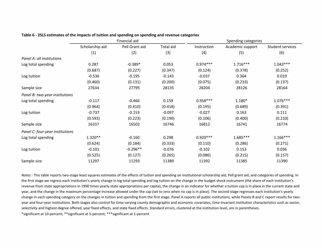
Table6-2SLSestimatesoftheimpactsoftuitionandspendingonspendingandrevenuecategories

Scholarshipaid PellGrantaid Totalaid Instruction Academicsupport Studentservices(1) (2) (3) (4) (5) (6)

PanelA:allinstitutionsLogtotalspending 0.287 -0.389* 0.053 0.974*** 1.716*** 1.043***

(0.687) (0.227) (0.347) (0.124) (0.378) (0.252)Logtuition -0.536 -0.195 -0.143 -0.037 0.364 0.019

(0.460) (0.131) (0.200) (0.075) (0.233) (0.137)Samplesize 27634 27795 28135 28204 28126 28164

PanelB:two-yearinstitutionsLogtotalspending -0.117 -0.466 0.159 0.958*** 1.180* 1.076***

(0.964) (0.410) (0.418) (0.195) (0.689) (0.391)Logtuition -0.737 -0.153 -0.097 -0.027 0.163 0.111

(0.593) (0.223) (0.190) (0.106) (0.400) (0.210)Samplesize 16337 16502 16746 16812 16741 16774

PanelC:four-yearinstitutionsLogtotalspending 1.320** -0.160 0.298 0.920*** 1.685*** 1.166***

(0.624) (0.184) (0.333) (0.110) (0.286) (0.271)Logtuition -0.101 -0.296** -0.076 -0.102 0.153 0.036

(0.525) (0.127) (0.265) (0.086) (0.215) (0.157)Samplesize 11297 11293 11389 11392 11385 11390

*significantat10-percent;**significantat5-percent;***significantat1-percent

Notes :Thistablereportstwo-stageleastsquaresestimatesoftheeffectsoftuitionandspendingoninstitutionalscholarshipaid,Pellgrantaid,andcategoriesofspending.Inthefirststageweregresseachinstitution'syearlychangeinlogtotalspendingandlogtuitiononthechangeinthebudgetshockinstrument(theshareofeachinstitution’srevenuefromstateappropriationsin1990timesyearlystateappropriationspercapita),thechangeinanindicatorforwhetheratuitioncapisinplaceinthecurrentstateandyear,andthechangeinthemaximumpercentageincreaseallowedunderthecap(settozerowhennocapisinplace).Thesecondstageregresseseachinstitution'syearlychangeineachspendingcategoryonthechangesintuitionandspendingfromthefirststage.PanelAreportsallpublicinstitutions,whilePanelsBandCreportresultsfortwo-yearandfour-yearinstitutions.Bothstagesalsocontrolfortime-varyingcountydemographicandeconomiccovariates,time-invariantinstitutioncharacteristicssuchassector,selectivityandhighestdegreeoffered,yearfixedeffects,andstatefixedeffects.Standarderrors,clusteredattheinstitutionlevel,areinparentheses.

Financialaid Spendingcategories

References

Angrist, J., D. Lang, and P. Oreopoulos (2009): “Incentives and services for college achievement:

evidence from a randomized trial,” American Economic Journal: Applied Economics, 1, 136–163.

Angrist, J. D. and J.-S. Pischke (2009): Mostly Harmless Econometrics, Princeton, NJ: Princeton

University Press.

Autor, D. H. (2014): “Skills, education, and the rise of earnings inequality among the other 99 percent,”

Science, 344, 843–851.

Autor, D. H., D. Dorn, and G. H. Hanson (2013): “The China syndrome: local labor market effects

of import competition in the United States,” American Economic Review, 103, 2121–2168.

Avery, C. and S. Turner (2012): “Student loans: do college students borrow too much – or not enough?”

The Journal of Economic Perspectives, 26, 165–192.

Bahr, P. R. (2014): “The labor market return in earnings to community college credits and credentials in

California,” Working paper, Center for the Study of Higher and Postsecondary Education.

Bahr, P. R., J. L. Gross, K. E. Slay, and R. D. Christensen (2013): “First in line: student regis-

tration priority in community colleges,” Educational Policy, 29, 342–374.

Barr, A. and S. E. Turner (2013): “Expanding enrollments and contracting state budgets: the effect

of the great recession on higher education,” The Annals of the American Academy of Political and Social

Science, 650, 168–193.

Barrow, L., L. Richburg-Hayes, C. E. Rouse, and T. Brock (2014): “Paying for performance: the

education impacts of a community college scholarship program for low-income adults,” Journal of Labor

Economics, 32, 563–599.

Bartik, T. J. (1991): Who Benefits from State and Local Economic Development Policies?, Kalamazoo,

MI: W. E. Upjohn Institute for Employment Research.

Baum, S. and J. Ma (2014): “Trends in college pricing,” College Board, Trends in Higher Education Series.

Bell, A. C., J. Carnahan, and H. P. L’Orange (2011): “State tuition, fees, and financial assistance

policies for public colleges and universities, 2010-11,” Report, State Higher Education Executive Officers

Association.

Bennett, W. J. (1987): “Our greedy colleges,” The New York Times, February 18th.

Bettinger, E. and R. Baker (2011): “The effects of student coaching in college: An evaluation of a

randomized experiment in student mentoring,” Tech. rep., National Bureau of Economic Research.

36

Bettinger, E. P. and B. T. Long (2009): “Addressing the needs of underprepared students in higher

education: does college remediation work?” Journal of Human Resources, 44, 736–771.

Blanchard, O. and L. Katz (1992): “Regional evolutions,” Brookings Papers on Economic Activity, 23,

1–76.

Bound, J., M. F. Lovenheim, and S. Turner (2010): “Why have college completion rates declined? An

analysis of changing student preparation and collegiate resources,” American Economic Journal: Applied

Economics, 2, 129–57.

——— (2012): “Increasing time to baccalaureate degree in the United States,” Education Finance and Policy,

7, 375–424.

Bound, J. and S. Turner (2007): “Cohort crowding: how resources affect collegiate attainment,” Journal

of Public Economics, 91, 877–899.

Card, D. (2001): “Immigrant inflows, native outflows, and the local market impacts of higher immigration,”

Journal of Labor Economics, 19, 22–64.

Card, D. and A. B. Krueger (1992): “Does school quality matter? Returns to education and character-

istics of public schools in the United States,” The Journal of Political Economy, 100, 1–40.

Carrell, S. E. and B. Sacerdote (2013): “Why do college going interventions work?” Tech. rep.,

National Bureau of Economic Research.

Cellini, S. R. (2009): “Crowded colleges and college crowd-out: The impact of public subsidies on the

two-year college market,” American Economic Journal: Economic Policy, 1, 1–30.

——— (2010): “Financial aid and for-profit colleges: does aid encourage entry?” Journal of Policy Analysis

and Management, 29, 526–552.

Cellini, S. R. and C. Goldin (2014): “Does federal student aid raise tuition? New evidence on for-profit

colleges,” American Economic Journal: Economic Policy, 6, 174–206.

Chetty, R., J. N. Friedman, E. Saez, N. Turner, and D. Yagan (2017): “Mobility report cards: the

role of colleges in intergenerational mobility,” Working paper.

Cohodes, S. R. and J. S. Goodman (2014): “Merit aid, college quality, and college completion: Mas-

sachusetts’ Adams scholarship as an in-kind subsidy,” American Economic Journal: Applied Economics,

6, 251–285.

Delaney, J. A. and W. R. Doyle (2011): “State spending on higher education: testing the balance wheel

over time,” Journal of Education Finance, 36, 343–368.

37

Deming, D. and S. Dynarski (2010): “College aid,” in Targeting Investments in Children: Fighting

Poverty When Resources are Limited, ed. by P. B. Levine and D. J. Zimmerman, Chicago, IL: University

of Chicago Press, chap. 10, 283–302.

Deming, D. J. (2017): “Increasing college completion with a federal higher education matching grant,” The

Hamilton Project, Policy Proposal 2017-03.

Dynarski, S. (2008): “Building the stock of college-educated labor,” Journal of Human Resources, 43,

576–610.

Ehrenberg, R. G. (2012): “American higher education in transition,” The Journal of Economic Perspec-

tives, 26, 193–216.

Fitzpatrick, M. D. and D. Jones (2012): “Higher education, merit-based scholarships and post-

baccalaureate migration,” Tech. rep., National Bureau of Economic Research.

Gennaioli, N., R. L. Porta, F. L. de Silanes, and A. Shleifer (2013): “Human capital and regional

development,” Quarterly Journal of Economics, 128, 105–164.

Ginsberg, B. (2011): The Fall of the Faculty, Oxford University Press.

Hanushek, E. A., J. Ruhose, and L. Woessmann (forthcoming): “Knowledge capital and aggregate

income differences: development accounting for US states,” American Economic Journal: Macroeconomics.

Hanushek, E. A. and L. Woessmann (2008): “The role of cognitive skills in economic development,”

Journal of Economic Literature, 46, 607–668.

Hemelt, S. W. and D. E. Marcotte (2011): “The impact of tuition increases on enrollment at public

colleges and universities,” Educational Evaluation and Policy Analysis, 33, 435–457.

Jackson, C. K., R. C. Johnson, and C. Persico (2016): “The effects of school spending on educational

and economic outcomes: evidence from school finance reforms,” Quarterly Journal of Economics, 131,

157–218.

Jacob, B., B. McCall, and K. M. Stange (2013): “College as country club: do colleges cater to students’

preferences for consumption?” NBER working paper no. 18745.

Jaquette, O. and E. Parra (2016): “The problem with the Delta Cost Project database,” Research in

Higher Education, 57, 1–22.

Kane, T. J., P. Orszag, and D. L. Gunter (2003): “State fiscal constraints and higher education

spending: the role of Medicaid and the business cycle,” Urban Institute Discussion Paper no. 11.

Lafortune, J., J. Rothstein, and D. W. Schanzenbach (2016): “School finance reform and the

distribution of student achievement,” Working paper.

38

Levin, H. M., E. Garcia, and J. Morgan (2012): “Cost-effectiveness of Accelerated Study in Associate

Programs (ASAP) of the City University of New York (CUNY),” Technical report, Center for Benefit-Cost

Studies of Education, Columbia University Teachers College.

Malani, A. and J. Reif (2015): “Interpreting pre-trends as anticipation: impact on estimated treatment

effects from tort reform,” Journal of Public Economics, 124, 1–17.

National Center for Education Statistics (2015a): “Digest of education statistics 2015,” Institute of

Education Sciences report.

——— (2015b): “The Nation’s Report Card: 2015 Mathematics and Reading Assessments,” National As-

sessment of Educational Progress report.

OECD (2013): “OECD Skills Outlook 2013: First Results from the Survey of Adult Skills,”

http://dx.doi.org/10.1787/9789264204256-en.

Parmley, K., A. Bell, H. L’Orange, and P. Lingenfelter (2009): “State budgeting for higher

education in the united states,” Report, State Higher Education Executive Officers.

Scrivener, S., M. J. Weiss, A. Ratledge, T. Rudd, C. Sommo, and H. Fresques (2015): “Doubling

graduation rates: three-year effects of CUNY’s Accelerated Study in Associate Programs (ASAP) for

developmental education students,” Report, MDRC.

Seftor, N. S. and S. Turner (2002): “Back to school: Federal student aid policy and adult college

enrollment,” Journal of Human Resources, 37, 336–352.

Turner, L. J. (2013): “The road to Pell is paved with good intentions: the economic incidence of Federal

student grant aid,” Working paper.

Turner, S. (2004): “Going to college and finishing college: explaining different educational outcomes,” in

College Choices: The Economics of Where to Go, When to Go, and How to Pay for it, ed. by C. M.

Hoxby, Chicago, IL: University of Chicago Press, chap. 1, 13–62.

39

FigureA1-Evolutionofappropriationsforfourlargestates

Notes:Thisfigureplotstrendsinstateappropriationsforhighereducationpercollege-agepopulationforCalifornia,FloridaNewYorkandTexas.DatacomefromtheIntegratedPostsecondaryEducationDataSystem(IPEDS)for1990-2013.

2000

3000

4000

5000

6000

1990 1995 2000 2005 2010 2015

California FloridaNew York Texas

Source: IPEDS

State Appropriations Per Age 19-23 Population, 1990-2013Trend in Higher Education Funding in Four Large States

FigureA2

Notes: Thisfigurepresentsestimatesand95percentconfidenceintervalsfromaregressionoftotalenrollment(inlevels)forpublicinstitutionsonlagsandleadsofthestatebudgetshockinstrument(theshareofeachinstitution’srevenuefromstateappropriationsin1990timesyearlystateappropriationspercapita,in$1000s),anindicatorforwhetheratuitioncapisinplace,andthemaximumpercentageincreaseallowedunderthecap(settozerowhennocapisinplace).Themodelalsocontrolsforlagsandleadsofcountyandstateunemploymentrates,time-varyingcountyandinstitutioncharacteristics,institutionfixedeffects,yearfixedeffects,andstate-specifictimetrends.Standarderrorsareclusteredattheinstitutionlevel.

-200

020

0

-4 -3 -2 -1 0 1 2 3 4 5

Impact of Budget Shock on Total Enrollment-4

000

400

-4 -3 -2 -1 0 1 2 3 4 5

Impact of Having a Tuition Cap on Total Enrollment

-400

00

4000

-4 -3 -2 -1 0 1 2 3 4 5Event Time

Impact of Maximum Tuition Cap on Total Enrollment

FigureA3

Notes: Thisfigurepresentsestimatesand95percentconfidenceintervalsfromaregressionoftotaldegreesawarded(inlevels)onlagsandleadsofthestatebudgetshockinstrument(theshareofeachinstitution’srevenuefromstateappropriationsin1990timesyearlystateappropriationspercapita,in$1000s),anindicatorforwhetheratuitioncapisinplace,andthemaximumpercentageincreaseallowedunderthecap(settozerowhennocapisinplace).Themodelalsocontrolsforlagsandleadsofcountyandstateunemploymentrates,time-varyingcountyandinstitutioncharacteristics,institutionfixedeffects,yearfixedeffects,andstate-specifictimetrends.Standarderrorsareclusteredattheinstitutionlevel.

-60

060

-4 -3 -2 -1 0 1 2 3 4 5

Impact of Budget Shock on Total Degrees and Certificates

-60

060

-4 -3 -2 -1 0 1 2 3 4 5

Impact of Having a Tuition Cap on Total Degrees and Certificates

-600

060

0

-4 -3 -2 -1 0 1 2 3 4 5Event Time

Impact of Maximum Tuition Cap on Total Degrees and Certificates

TableA1-Listoftuitioncapsandfreezesbystate,1990-20131990 1991 1992 1993 1994 1995 1996 1997 1998 1999 2000 2001 2002 2003 2004 2005 2006 2007 2008 2009 2010 2011 2012 2013

Alabama2 -- -- -- -- -- -- -- -- -- -- -- -- -- -- -- -- 0 0 0 0 0 -- -- --Alaska -- -- -- -- -- -- -- -- -- -- -- -- -- -- -- -- -- -- -- -- -- -- -- --Arizona -- -- -- -- -- -- -- -- -- -- -- -- -- -- -- -- -- -- -- -- -- -- -- --Arkansas -- -- -- -- -- -- -- -- -- -- -- -- -- -- -- -- -- -- -- -- -- -- -- --California -- -- -- -- -- -- -- -- -- -- -- -- -- -- -- -- -- -- -- -- -- -- -- --Colorado -- -- -- -- -- -- -- -- -- -- -- -- -- -- -- -- -- -- -- -- -- -- -- --Connecticut1 -- -- -- -- -- -- -- -- -- -- 0 -- -- -- -- -- -- -- -- -- -- -- 0 --Delaware -- -- -- -- -- -- -- -- -- -- -- -- -- -- -- -- -- -- -- -- -- -- -- --Florida -- -- -- -- -- 0 -- -- -- -- -- -- -- -- -- -- -- -- 0 -- -- -- -- --Georgia -- -- -- -- -- -- -- -- -- -- -- -- -- -- -- -- -- -- -- -- -- -- -- --Hawaii -- -- -- -- -- -- -- -- -- -- -- -- -- -- -- -- -- -- -- -- -- -- -- --Idaho -- -- -- -- -- -- -- -- -- -- -- -- -- 0.1 0.1 0.1 0.1 0.1 0.1 0.1 0.1 -- 0.1 0.1Illinois -- -- -- -- -- -- -- -- -- -- -- -- -- -- -- -- -- -- -- -- -- -- -- --Indiana -- -- -- -- -- -- -- -- -- -- -- -- -- -- -- -- -- -- -- -- -- -- -- --Iowa -- -- -- -- -- -- -- -- -- -- -- -- -- -- -- -- -- -- -- -- -- -- -- --Kansas -- -- -- -- -- -- -- -- -- -- -- -- -- -- -- -- -- -- -- -- -- -- -- --Kentucky -- -- -- -- -- -- -- -- -- -- -- -- -- -- -- -- -- -- -- -- -- -- -- --Louisiana -- -- -- -- -- -- -- -- -- -- -- -- -- -- -- -- -- -- -- -- -- -- -- --Maine2 -- -- -- -- -- -- -- -- -- -- 0 0 0 0 0 0 -- -- -- -- -- 0 -- 0Maryland1 -- -- -- -- -- -- -- -- 0.04 0.04 0.04 0.04 0.04 -- -- -- -- 0 0 0 0 0.03 0.03 0.03Massachusetts -- -- -- -- -- -- -- -- -- -- -- -- -- -- -- -- -- -- -- -- -- -- -- --Michigan -- -- -- -- -- -- -- -- -- -- -- -- -- -- -- -- -- -- -- -- -- -- -- --Minnesota -- -- -- -- -- -- -- -- -- -- -- -- -- -- -- -- -- -- -- -- -- -- -- --Mississippi -- -- -- -- -- -- -- -- -- -- -- -- -- -- -- -- -- -- -- -- -- -- -- --Missouri1 -- -- -- -- -- -- -- -- -- -- -- -- -- -- -- -- -- -- -- -- 0 0 -- --Montana -- -- -- -- -- -- -- -- -- -- -- -- -- -- -- -- -- -- 0 0 -- -- -- --Nebraska -- -- -- -- -- -- -- -- -- -- -- -- -- -- -- -- -- -- -- -- -- -- -- --Nevada -- -- -- -- -- -- -- -- -- -- -- -- -- -- -- -- -- -- -- -- -- -- -- --NewHampshire2 -- -- -- -- -- -- -- -- -- -- -- -- -- -- -- -- -- 0 -- 0 -- -- -- 0NewJersey1 -- -- -- -- -- -- -- -- -- -- -- -- -- -- 0.09 0.08 0.08 0.08 -- -- 0.03 0.04 -- --NewMexico -- -- -- -- -- -- -- -- -- -- -- -- -- -- -- -- -- -- -- -- -- -- -- --NewYork3 -- -- -- -- 0 0 -- 0 0 0 0 0 0 0 -- 0 0 0 0 0 -- -- -- --NorthCarolina1 -- -- -- -- -- -- -- -- -- -- -- -- -- -- -- -- 0 -- -- 0 -- -- 0.065 --NorthDakota -- -- -- -- -- -- -- -- -- -- -- -- -- -- -- -- -- -- -- -- -- -- -- --Ohio -- -- -- -- 0.06 0.06 0.06 0.06 0.06 0.06 0.06 0.06 0.06 -- -- -- 0.06 0.06 0.035 0.035 0.035 0.035 0.035 0.035Oklahoma4 -- -- -- -- -- -- -- -- -- -- -- -- 0.07 0.07 -- -- -- -- -- -- 0 -- -- --Oregon1 -- -- -- -- -- -- -- -- 0 0 0 0 -- -- -- -- 0.03 0.03 -- -- -- -- -- --Pennsylvania -- -- -- -- -- -- -- -- -- -- -- -- -- -- -- -- -- -- -- -- -- -- -- --RhodeIsland -- -- -- -- -- -- -- -- -- -- -- -- -- -- -- -- -- -- -- -- -- -- -- --SouthCarolina -- -- -- -- -- -- -- -- -- -- -- -- -- -- -- -- -- -- -- -- -- -- -- --SouthDakota -- -- -- -- -- -- -- -- -- -- -- -- -- -- -- -- -- -- -- -- -- -- -- --Tennessee -- -- -- -- -- -- -- -- -- -- -- -- -- -- -- -- -- -- -- -- -- -- -- --Texas -- -- -- -- -- -- -- -- -- -- -- -- -- -- -- -- -- -- -- -- -- -- -- --Utah -- -- -- -- -- -- -- -- -- -- -- -- -- -- -- -- -- -- -- -- -- -- -- --Vermont -- -- -- -- -- -- -- -- -- -- -- -- -- -- -- -- -- -- -- -- -- -- -- --Virginia -- -- -- -- -- 0.03 0.03 0 0 0 -0.2 0 0 -- -- -- -- -- 0.06 0.04 -- -- -- --Washington -- -- -- -- -- -- -- -- -- -- -- -- -- -- -- -- -- -- -- -- -- -- -- --WestVirginia -- -- -- -- -- -- -- -- -- -- -- -- -- -- -- -- -- -- -- -- -- -- -- --Wisconsin1 -- -- -- -- -- -- -- -- -- -- -- 0 -- 0.08 -- -- -- -- -- -- -- -- 0.055 0.055Wyoming -- -- -- -- -- -- -- -- -- -- -- -- -- -- -- -- -- -- -- -- -- -- -- --Notes :Thistablelistsstatesandyearswherestatelegislaturesimposein-statetuitioncapsandfreezesatpublicinstitutions.Wecompiledthesedatabyreferencingofficialsourceswhenavailable,combinedwithLexis-Nexissearchesofstatenewspapersgoingbackto1990.Insomecaseswecheckedactualtuitiondatatoconfirmtheimpositionofacap,althoughinnocasedidwecodeatuitioncaporfreezeunlessitcouldbeindependentlyverified.1-Appliesonlytofour-yearinstitutionsinthestate.2-Appliesonlytotwo-yearinstitutionsinthestate.3-AppliesonlytoCUNY(except2003)andCornell(allyears).4-AppliestoallinstitutionsexcepttheOklahomaTechnologyCenters.

All Twoyear Fouryear(1) (2) (3)

Twoyear -0.457***(0.107)

Selective -0.667***(0.124)

Asashareoftotalspending:Tuitionandfees 0.134*** -0.018 0.276***

(0.029) (0.040) (0.060)Stateappropriations 0.605*** 0.472*** 0.628***

(0.029) (0.052) (0.043)Localappropriations -0.399*** -0.337*** -0.031*

(0.034) (0.055) (0.018)Totalgrants 0.040*** 0.028 0.151***

(0.015) (0.018) (0.030)Instructionalspending 0.067*** 0.062*** 0.156***

(0.016) (0.020) (0.030)Academicsupport 0.022*** 0.011 0.021

(0.006) (0.008) (0.014)Studentservices 0.012* 0.002 0.050***

(0.007) (0.008) (0.018)Administration -0.012 -0.030*** 0.055***

(0.009) (0.010) (0.019)Scholarships 0.013* 0.017* 0.069***

(0.008) (0.010) (0.013)

Logtotalspending -0.612*** -0.204 -2.884***(0.203) (0.130) (0.381)

Logenrollment -0.322 -0.572* -0.699(0.242) (0.342) (0.455)

Samplesize 30072 17568 12504

*significantat10-percent;**significantat5-percent;***significantat1-percent

TableA2-Correlatesofrelianceonstateappropriations

Notes: Thistabledescribesrelationshipsbetweenpublicinstitutioncharacteristicsandrelianceonstateappropriations,definedastheshareofeachinstitution’srevenuefromstateappropriationsin1990.Eachrowshowsthecoefficientfromaregressionofacharacteristiconthismeasureofrelianceusingdatafrom1991-2013,controllingforstateeffectsandyeareffects.Column(1)showsresultsforallpublicinstitutions,column(2)showsresultsfortwoyearinstitutions,andcolumn(3)showsresultsforfouryearinstitutions.Standarderrors,clusteredattheinstitutionlevel,areinparentheses.

TableA3-2SLSestimatesoftheimpactsoftuitionandspendingonotherenrollmentoutcomes

Currentyear T+1 T+2 T+3TwoYearInstitutionsPanelA:logFTUGenrollment (1) (2) (3) (4)Logtotalspending 0.129 0.130 0.083 0.049

(0.282) (0.353) (0.366) (0.322)Logtuition -0.021 -0.094 -0.019 -0.200

(0.151) (0.177) (0.193) (0.187)

Samplesize 16797 16107 15387 14662

PanelB:logPTUGenrollmentLogtotalspending 0.406 1.787*** 1.852*** 1.672***

(0.475) (0.547) (0.591) (0.517)Logtuition -0.175 0.251 0.246 -0.035

(0.214) (0.305) (0.323) (0.293)Samplesize 16750 16060 15341 14618

FourYearInstitutionsPanelC:logFTUGenrollmentLogtotalspending 0.071 0.384*** 0.246 0.182

(0.090) (0.148) (0.150) (0.172)Logtuition -0.080 0.040 -0.065 -0.100

(0.065) (0.103) (0.094) (0.100)

Samplesize 11391 10844 10293 9755

PanelD:logPTUGenrollmentLogtotalspending 0.572** 0.283 1.106*** 0.786*

(0.270) (0.311) (0.333) (0.422)Logtuition 0.173 -0.399* -0.276 -0.629**

(0.241) (0.239) (0.251) (0.312)

Samplesize 11353 10804 10253 9715

*significantat10-percent;**significantat5-percent;***significantat1-percent

Notes :Thistablereportstwo-stageleastsquaresestimatesoftheeffectsoftuitionandspendingonlogfull-timeandpart-timeundergraduateenrollmentatfour-yearinstitutions.Inthefirststageweregresseachinstitution'syearlychangeinlogtotalspendingandlogtuitiononthechangeinthebudgetshockinstrument(theshareofeachinstitution’srevenuefromstateappropriationsin1990timesyearlystateappropriationspercapita),thechangeinanindicatorforwhetheratuitioncapisinplaceinthecurrentstateandyear,andthechangeinthemaximumpercentageincreaseallowedunderthecap(settozerowhennocapisinplace).Thesecondstageregresseseachinstitution'syearlychangeinlogenrollmentonchangesintuitionandspendingfromthefirststage.PanelAreportsresultsforfull-timeundergraduateenrollmentandPanelBreportsresultsforparttimeenrollment.PanelsAandBrestrictthesampletotwo-yearinstitutions,whilePanelsCandDrepeatthepatternforfour-yearinstitutions.Bothstagesalsocontrolfortime-varyingcountydemographicandeconomiccovariates,time-invariantinstitutioncharacteristicssuchassector,selectivityandhighestdegreeoffered,yearfixedeffects,andstatefixedeffects.Standarderrors,clusteredattheinstitutionlevel,areinparentheses.

TableA4-2SLSestimatesoftheimpactsofspendingandtuitiononenrollmentbyrace

Currentyear T+1 T+2 T+3PanelA:non-whites (1) (2) (3) (4)Logtotalspending 0.113 0.787*** 0.854*** 0.857***

(0.144) (0.207) (0.228) (0.233)Logtuition -0.119 0.086 0.031 -0.038

(0.082) (0.119) (0.134) (0.142)Samplesize 28197 26958 25687 24422

PanelB:whitesLogtotalspending 0.481*** 0.857*** 0.905*** 0.874***

(0.146) (0.188) (0.219) (0.221)Logtuition 0.076 0.070 0.055 -0.079

(0.081) (0.104) (0.124) (0.131)Samplesize 28189 26950 25679 24414

*significantat10-percent;**significantat5-percent;***significantat1-percent

Notes :Thistablereportstwo-stageleastsquaresestimatesoftheeffectsoftuitionandspendingonlogenrollmentfornon-whiteandwhitestudents.Inthefirststageweregresseachinstitution'syearlychangeinlogtotalspendingandlogtuitiononthechangeinthebudgetshockinstrument(theshareofeachinstitution’srevenuefromstateappropriationsin1990timesyearlystateappropriationspercapita),thechangeinanindicatorforwhetheratuitioncapisinplaceinthecurrentstateandyear,andthechangeinthemaximumpercentageincreaseallowedunderthecap(settozerowhennocapisinplace).Thesecondstageregresseseachinstitution'syearlychangeinlognon-whiteenrollmentorlogwhiteenrollmentonthechangesintuitionandspendingfromthefirststage.Bothstagesalsocontrolfortime-varyingcountydemographicandeconomiccovariates,time-invariantinstitutioncharacteristicssuchassector,selectivityandhighestdegreeoffered,yearfixedeffects,andstatefixedeffects.Standarderrors,clusteredattheinstitutionlevel,areinparentheses.

TableA5-2SLSestimatesbyfour-yearcollegeselectivity

PanelA:lessselective Currentyear T+1 T+2 T+3Logenrollment (1) (2) (3) (4)Logtotalspending 0.299** 0.541** 0.814** 0.747**

(0.151) (0.244) (0.328) (0.355)Logtuition 0.024 -0.021 0.075 0.078

(0.087) (0.131) (0.206) (0.201)Samplesize 4558 4362 4165 3969

LogtotalawardsLogtotalspending 0.441 0.727 1.035** 0.829*

(0.352) (0.456) (0.461) (0.472)Logtuition 0.158 0.441 0.663** 0.652**

(0.212) (0.300) (0.328) (0.323)Samplesize 4503 4307 4111 3916

PanelB:moreselectiveLogenrollmentLogtotalspending 0.229* 0.417** 0.615*** 0.469*

(0.118) (0.208) (0.231) (0.261)Logtuition -0.016 -0.077 -0.066 -0.176

(0.093) (0.137) (0.162) (0.172)Samplesize 5980 5713 5442 5173SamplesizeLogtotalawardsLogtotalspending 0.337 0.254 0.441 0.556

(0.267) (0.329) (0.333) (0.383)Logtuition 0.183 0.045 0.072 0.286

(0.207) (0.200) (0.225) (0.235)Samplesize 5964 5691 5420 5152Samplesize

*significantat10-percent;**significantat5-percent;***significantat1-percent

Notes :Thistablereportstwo-stageleastsquaresestimatesoftheeffectsoftuitionandspendingoncertificatesanddegreesawardedbyselectivityforfour-yearinstitutions.Moreselectiveinstitutionsarethosewithadmissionrateslessthan60percent,instatestudentshareslessthan90percent,and2009Barronsrankingsofoneortwo.Lessselectiveinstitutionsarethosewithadmissionsratesabove60percent,instatesharesabove90percent,andBarronsrankingsabovetwo.Inthefirststageweregresseachinstitution'syearlychangeinlogtotalspendingandlogtuitiononthechangeinthebudgetshockinstrument(theshareofeachinstitution’srevenuefromstateappropriationsin1990timesyearlystateappropriationspercapita),thechangeinanindicatorforwhetheratuitioncapisinplaceinthecurrentstateandyear,andthechangeinthemaximumpercentageincreaseallowedunderthecap(settozerowhennocapisinplace).Thesecondstageregresseseachinstitution'syearlychangeincertificatesordegreesonthechangesintuitionandspendingfromthefirststage.PanelsAandBreportresultsforless-andmore-selectivefour-yearinstitutions.Bothstagesalsocontrolfortime-varyingcountydemographicandeconomiccovariates,time-invariantinstitutioncharacteristicssuchassector,selectivityandhighestdegreeoffered,yearfixedeffects,andstatefixedeffects.Standarderrors,clusteredattheinstitutionlevel,areinparentheses.

TableA6-Alternativestate-by-timecontrolsLogSpending LogTuition

(1) (2)Changes,stateeffects 0.300** -0.017(baselinemodel) (0.134) (0.076)

Changes,statetrends 0.268 -0.037(0.166) (0.080)

Changes,state-by-four-yeareffects 0.244 -0.046(0.158) (0.081)

Changes,institutioneffects 0.330** -0.014(0.145) (0.075)

Levels,institutioneffects 0.417*** -0.051(0.081) (0.164)

Levels,institutioneffects 0.380*** -0.111andstatetrends (0.124) (0.104)

Levels,institutioneffects 0.287 -0.160andstate-by-four-yeareffects (0.274) (0.212)

Samplesize

*significantat10-percent;**significantat5-percent;***significantat1-percent

Notes :Thistablereportstwo-stageleastsquaresestimatesoftheeffectsoftuitionandspendingonlogtotalfallenrollmentwithalternativecontrolsforstate-by-timevariationinoutcomes."Changes"specificationsusetheyearlychangeinlogenrollmentasthedependentvariableandchangesinlogtuitionandlogspendingastheendogenousregressors,instrumentingwiththechangeinthebudgetshockinstrument,thechangeinwhetheratuitioncapisinplace,andthechangeinthemaximumpercentageincreaseallowedunderthecap(settozerowhennocapisinplace)."Levels"specificationsuselogenrollmentasthedependentvariable,logtuitionandlogspendingasendogenousregressors,andthebudgetshock,presenceofatutioncap,andlevelofthecapasinstruments."Changes"modelscontrolfortime-varyingcountydemographicandeconomiccovariates,time-invariantinstitutioncharacteristics,andyeareffects,while"levels"modelscontrolsfortime-varyingcountydemographicandeconomiccovariates,institutioncharacteristicsinteractedwithatimetrend,andyeareffects.Standarderrors,clusteredattheinstitutionlevel,areinparentheses.

Outcomeislogenrollment

27659

TableA7-2SLSestimatesoftheeffectsofspendingandtuitionbasedonappropriations

Currentyear T+1 T+2 T+3PanelA:logenrollment (1) (2) (3) (4)Logtotalspending 0.331*** 0.563*** 0.480*** 0.344***

(0.095) (0.079) (0.080) (0.064)Logtuition -0.021 0.030 -0.031 -0.139

(0.064) (0.077) (0.087) (0.095)Samplesize 28197 26958 25687 24422

PanelB:logtotalawardsLogtotalspending 0.473*** 0.666*** 0.514*** 0.483***

(0.123) (0.120) (0.119) (0.104)Logtuition 0.153 0.207 0.111 -0.041

(0.131) (0.146) (0.146) (0.149)Samplesize 28108 26834 25564 24304

*significantat10-percent;**significantat5-percent;***significantat1-percent

Notes :Thistablereportstwo-stageleastsquaresestimatesoftheeffectsoftuitionandspendingontotalenrollmentandlogtotalawardsusingactualappropriationsratherthanthebudgetshocktoinstrumentforspending.Inthefirststageweregresseachinstitution'syearlychangeinlogspendingandlogtuitiononthechangeintheiractuallogappropriations,thechangeinanindicatorforwhetheratuitioncapisinplaceinthecurrentstateandyear,andthechangeinthemaximumpercentageincreaseallowedunderthecap(settozerowhennocapisinplace).Thesecondstageregresseseachinstitution'syearlychangesinoutcomesonpredictedchangesinlogspendingandtuitionfromthefirststage.PanelAreportsresultsforlogenrollment,andPanelBreportsresultsforlogtotalawards.Bothstagesalsocontrolfortime-varyingcountydemographicandeconomiccovariates,time-invariantinstitutioncharacteristicssuchassector,selectivityandhighestdegreeoffered,yearfixedeffects,andstatefixedeffects.Standarderrors,clusteredattheinstitutionlevel,areinparentheses.

TableA8-Spilloverimpactsofpublicbudgetshocksonprivateinstitutions,byawardtypePanelA:logcertificates Currentyear T+1 T+2 T+3

(1) (2) (3) (4)Countyaveragebudgetshock -0.024 -0.052* -0.018 -0.010

(0.025) (0.030) (0.037) (0.041)Anytuitioncap -0.013 -0.014 -0.005 -0.029*

(0.013) (0.015) (0.016) (0.017)Samplesize 33507 29403 25844 22701

PanelB:logassociate'sdegreesCountyaveragebudgetshock -0.106*** -0.202*** -0.115* -0.083

(0.040) (0.050) (0.061) (0.065)Anytuitioncap 0.011 0.033* 0.024 0.002

(0.018) (0.020) (0.022) (0.024)Samplesize 16969 15148 13490 11957

PanelC:logbachelor'sdegreesCountyaveragebudgetshock 0.013 0.000 -0.063 -0.021

(0.041) (0.044) (0.052) (0.054)Anytuitioncap 0.013 0.021 0.007 0.011

(0.012) (0.013) (0.015) (0.015)SampleSize 18966 17188 15547 13969

*significantat10-percent;**significantat5-percent;***significantat1-percent

Notes :Thistablereportsreducedformestimatesoftheimpactsofthechangeintheaverageenrollment-weightedbudgetshockinstrument(theshareofeachinstitution’srevenuefromstateappropriationsin1990timesyearlystateappropriationspercapita)acrosspublicinstitutionsinacountyandthechangeinanindicatorforwhetheranytuitioncapisinplaceinthecurrentstateandyearonthechangeinoutcomesinprivate(not-for-profitandfor-profit)institutionsinthesamecounty.PanelsA,B,andCreportresultsforlogcertificates,logassociate'sdegreesandlogbachelor'sdegreesrespectively.Theregressionsalsocontrolfortime-varyingcountydemographicandeconomiccovariates,time-invariantinstitutioncharacteristicssuchassector,selectivityandhighestdegreeoffered,yearfixedeffects,andstatefixedeffects.Standarderrors,clusteredattheinstitutionlevel,areinparentheses.

TableA9-Impactsofcounty-levelbudgetshocksonoutcomesinpublicinstitutionsPanelA:logenrollment Currentyear T+1 T+2 T+3

(1) (2) (3) (4)Logtotalspending 0.528** 0.824*** 1.141*** 0.996***

(0.209) (0.250) (0.312) (0.292)Logtuition 0.138 0.090 0.255 0.023

(0.130) (0.150) (0.192) (0.179)Samplesize 28197 26958 25687 24422

PanelB:logtotalawardsLogtotalspending 0.139 0.819** 1.312*** 1.171***

(0.337) (0.412) (0.483) (0.449)Logtuition 0.073 0.199 0.402 0.369

(0.210) (0.244) (0.298) (0.273)Samplesize 28108 26834 25564 24304

*significantat10-percent;**significantat5-percent;***significantat1-percent

Notes :Thistablereportsreducedformestimatesoftheimpactsofthechangeintheaverageenrollment-weightedbudgetshockinstrument(theshareofeachinstitution’srevenuefromstateappropriationsin1990timesyearlystateappropriationspercapita)acrosspublicinstitutionsinacountyandthechangeinanindicatorforwhetheranytuitioncapisinplaceinthecurrentstateandyearonthechangeinoutcomesforallpublicinstitutionsinacounty.PanelsAandBreportresultsforlogenrollmentandlogtotalawards.Theregressionsalsocontrolfortime-varyingcountydemographicandeconomiccovariates,time-invariantinstitutioncharacteristicssuchassector,selectivityandhighestdegreeoffered,yearfixedeffects,andstatefixedeffects.Standarderrors,clusteredattheinstitutionlevel,areinparentheses.

TableA10-2SLSestimatesofeffectsonfreshmanandupperclassmanenrollment

Currentyear T+1 T+2 T+3PanelA:logFTEfreshmenLogtotalspending 0.580* 0.032 1.276*** 0.829**

(0.349) (0.391) (0.480) (0.421)Logtuition 0.148 -0.206 0.713** 0.414

(0.194) (0.197) (0.281) (0.253)Samplesize 27311 26093 24841 23610

PanelB:logFTEupperclassmenLogtotalspending 1.298** 0.356 -0.299 1.676***

(0.589) (0.474) (0.464) (0.522)Logtuition 0.836** -0.231 -0.054 0.406

(0.373) (0.272) (0.272) (0.302)Samplesize 27896 26646 25364 24107

*significantat10-percent;**significantat5-percent;***significantat1-percent

Notes :Thistablereportstwo-stageleastsquaresestimatesoftheeffectsoftuitionandspendingonenrollmentforfreshmanandupperclassmen.Inthefirststageweregresseachinstitution'syearlychangeinlogtotalspendingandlogtuitiononthechangeinthebudgetshockinstrument(theshareofeachinstitution’srevenuefromstateappropriationsin1990timesyearlystateappropriationspercapita),thechangeinanindicatorforwhetheratuitioncapisinplaceinthecurrentstateandyear,andthechangeinthemaximumpercentageincreaseallowedunderthecap(settozerowhennocapisinplace).Thesecondstageregresseseachinstitution'syearlychangeincertificatesordegreesonthechangesintuitionandspendingfromthefirststage.PanelAreportsresultsforfull-timeequivalentfreshmen,andPanelBreportsresultsforupperclassmen(withpart-timestudentscountingas0.5inbothcases).Bothstagesalsocontrolfortime-varyingcountydemographicandeconomiccovariates,time-invariantinstitutioncharacteristicssuchassector,selectivityandhighestdegreeoffered,yearfixedeffects,andstatefixedeffects.Standarderrors,clusteredattheinstitutionlevel,areinparentheses.